First Passage Percolation in Hostile Environment with Recovery

Abstract

We study a natural modification of the process introduced in [SS19], known as first passage percolation in hostile environment. Consider a graph $G$ with a reference vertex $o$. Place a black particle at $o$ and colorless particles (seeds) at all other vertices. The black particle starts spreading a black first passage percolation of rate $1$, while all seeds are dormant. As soon as a seed is reached by the process, it gets active by turning red, and starts spreading a red first passage percolation, also of rate $1$. All vertices (except for $o$) are equipped with independent exponential clocks ringing at rate $\gamma>0$, when a clock rings the corresponding red vertex turns black. For $t\geq 0$, let $H_{t}$ and $M_{t}$ denote the size of the longest red path and of the largest red cluster present at time $t$. If $G$ is the semi-line, then for all $\gamma>0$ almost surely $\limsup_{t}\frac{H_{t}\log\log t}{\log t}=1$ and $\liminf_{t}H_{t}=0$. In contrast, if $G$ is an infinite Galton-Watson tree with offspring mean $\mathbf{m}>1$ then, for all $\gamma>0$, almost surely $\liminf_{t}\frac{H_{t}\log t}{t}\geq\mathbf{m}-1$ and $\liminf_{t}\frac{M_{t}\log\log t}{t}\geq\mathbf{m}-1$, while $\limsup_{t\to\infty}\frac{M_{t}}{e^{ct}}\leq 1$, for all $c>\mathbf{m}-1$. Furthermore, if we restrict our attention to bounded-degree graphs, then almost surely as $t\to\infty$, for all $\gamma>0$, $H_{t}$ is of order at most $t$. Moreover, for any $\varepsilon>0$ there is a critical value $\gamma_{c}>0$ so that for all $\gamma>\gamma_{c}$, almost surely $\limsup_{t}\frac{M_{t}}{t}\leq\varepsilon$.

Keywords: First passage percolation, first passage percolation in hostile environment, competition, recovery

1 Introduction

In this work we study a natural modification of the process known as First-passage percolation in hostile environment (FPPHE). Such process was initially introduced by Sidoravicius and Stauffer [SS19] as an auxiliary model to study the behavior of Multiparticle Diffusion Limited Aggregation in the high-density regime. However, FPPHE turned out to be an interesting model in its own right and it has attracted a lot of attention recently, as we review below.

Classical FPPHE process is defined as follows. Consider a locally finite and connected graph $G=(V,E)$ with a reference vertex $o$ that we call the origin. Fix a parameter, $\mu\in[0,1]$, and on each vertex $x\neq o$ independently, place a colorless particle with probability $\mu$ and no particle with probability $1-\mu$. We shall call these particles seeds. Now fix a new parameter $\lambda>0$.

At time $0$ place a particle at the origin, and let it initiate a first-passage percolation with rate $1$ (which we call $\text{FPP}_{1}$), while seeds are inactive (dormant). A seed remains inactive for as long as its hosting vertex has not been reached by first-passage percolation. When this occurs, the seed is activated, meaning that it turns red and originates a first-passage percolation with rate $\lambda$ (which we call $\text{FPP}_{\lambda}$). Note that a seed can be activated by either process ($\text{FPP}_{1}$ or $\text{FPP}_{\lambda}$), and once a vertex turns black (hosting $\text{FPP}_{1}$) or red (hosting $\text{FPP}_{\lambda}$), then it will stay so forever.

There are several natural questions about FPPHE. The first one is about finding conditions that ensure survival of $\text{FPP}_{1}$ or $\text{FPP}_{\lambda}$, that is, the possibility for $\text{FPP}_{1}$ or $\text{FPP}_{\lambda}$ to occupy an infinite connected component of the graph as time goes to infinity. Interestingly, the answer changes if we change the underlying properties of the graph. In [SS19] the authors show that on $\mathbb{Z}^{d}$ (for $d\geq 2$) for all $\lambda\in(0,1)$ and $\mu$ small enough, $\mathbb{P}(\text{FPP}_{1}\text{ survives})>0$, and if we condition on this event, then $\text{FPP}_{\lambda}$ dies out almost surely. On the other hand, [Fin21, Chapter 4] shows that for all $\lambda\geq 1$, $\text{FPP}_{1}$ dies out almost surely. When the underlying graph $G$ has fundamentally different structural properties, one can find completely different behaviors. For example, [CS21a] investigates the case of transitive, non-amenable, hyperbolic graphs. In such a setting, for all $\lambda>0$ and for all $\mu$ small enough, $\mathbb{P}(\text{FPP}_{1}\text{ survives})>0$; whereas $\text{FPP}_{\lambda}$ survives almost surely for all $\lambda>0$ and all $\mu\in(0,1)$. A natural next question is whether there might be a range of values for $\mu$ and for $\lambda$ so that there is coexistence, that is, when $\text{FPP}_{1}$ and $\text{FPP}_{\lambda}$ survive simultaneously. This question was answered in the positive in [FS22b] in the case of $\mathbb{Z}^{d}$ for $d\geq 3$ and in [CS21a] in the case of transitive, non-amenable, hyperbolic graphs.

This model is particularly challenging because in general one cannot rely on the property of monotonicity: intuitively, by adding more seeds, $\text{FPP}_{1}$ should be inhibited. However, in general this might not be true, as showed in [CS21b]. Although we believe monotonicity to hold at least when the underlying graph is transitive, there is yet no known proof of this fact.

In this note we look at the following natural modification of FPPHE. Consider a new parameter $\gamma>0$, which we call recovery rate, and on each vertex of the graph place independent exponential clocks (also independent of the process) that ring at rate $\gamma$. Whenever such a clock rings, if the corresponding vertex is hosting $\text{FPP}_{\lambda}$ then it switches to $\text{FPP}_{1}$, and nothing happens otherwise. In order to guarantee that the resulting process is well defined, throughout we will set $\lambda=1$. This avoids technical difficulties that can arise when a vertex recovers before spreading $\text{FPP}_{\lambda}$.

This natural model is motivated by the following interpretation. Suppose that $\text{FPP}_{\lambda}$ represents an infectious disease spreading through a network and that $\text{FPP}_{1}$ represents its cure and vertices of $G$ represent individuals in a community. Then, the recovery rate represents the rate at which a sick individual becomes healthy. Here we always assume that a recovered individual will not be able to be infected again. (Vertices switching from $\text{FPP}_{\lambda}$ to $\text{FPP}_{1}$ will stay so forever.) However, recovered individuals can spread the infection to neighboring sites (those hosting seeds).

We shall study the asymptotic behavior of the size of the longest path and of the largest cluster infected by $\text{FPP}_{\lambda}$ in two cases, namely when $G$ is the semi-line $\mathbb{N}$, and when $G$ is a supercritical Galton-Watson tree (including the trivial case of a homogeneous tree).

To our knowledge, this is the very first time that such a modification is analyzed for FPPHE, and we hope that this work will trigger further investigation in this direction.

1.1 Main results

From now on, we set the parameters characterizing FPPHE as $\lambda=1$ and $\mu=1$. The fact that $\text{FPP}_{\lambda}$ and $\text{FPP}_{1}$ spread at the same rate makes this model well defined, in the sense that when a vertex recovers before spreading $\text{FPP}_{\lambda}$ to its neighbors, there is no need to re-sample a new passage time. Moreover, $\mu=1$ considers the “most favorable” starting condition for $\text{FPP}_{\lambda}$, as every vertex (except for the origin) is occupied by a seed. It would be interesting to see how the value of $\mu\in(0,1)$ affects the (asymptotic) behavior of the largest size of a $\text{FPP}_{\lambda}$ cluster, however this is left for further investigation. In the following, we shall refer to “black” vertices as those occupied by $\text{FPP}_{1}$ and to “red” vertices as those occupied by $\text{FPP}_{\lambda}$.

For all $t\in\mathbb{R}$ let $H_{t}$ be the size of the longest (oriented) path consisting of $\text{FPP}_{\lambda}$ vertices (i.e., the longest red path) present at time $t$, and $M_{t}$ be the size of the largest $\text{FPP}_{\lambda}$ cluster (i.e., the biggest red cluster) present at time $t$. The present work focuses on the asymptotic behavior of $H_{t}$ and $M_{t}$ as $t\to\infty$, when $G$ is a tree (deterministic or random). More precisely, we show the following results.

Theorem 1.1.

When $G$ is the infinite semi-line $\mathbb{N}$ then, for all recovery rates $\gamma>0$,

• $\mathbb{P}\left(\limsup_{t\rightarrow+\infty}\frac{H_{t}\log\log t}{\log t}=1\right)=1$;

• $\mathbb{P}\left(\liminf_{t\rightarrow+\infty}H_{t}=0\right)=1$.

Roughly speaking, when $G=\mathbb{N}$ then the “largest” red component gets of order $\frac{\log t}{\log\log t}$, when $t$ is large. However, even if this event occurs infinitely often, it is not true that anything close to this size is maintained, as the second item shows. In fact, almost surely, there are arbitrary large times so that there is no red path in the graph, because all infected vertices have recovered. In contrast, the next theorem shows that whenever $G$ is a super-critical Galton-Watson tree with finite mean then eventually there will be non-trivial red paths (and red clusters) in the graph. More precisely, for all large times $t$, the longest red path is of order at least $\frac{t}{\log t}$ and the largest red cluster is of order at least $\frac{t}{\log\log t}$. The statement includes as well the “degenerate” case of a homogeneous tree of degree $d+1\geq 3$, whose distribution is Bin($d,1$).

Theorem 1.2.

If $G$ is a supercritical Galton-Watson tree whose offspring distribution has finite mean $\mathbf{m}>1$, then for all $\gamma>0$,

• $\displaystyle\mathbb{P}\left(\liminf_{t\rightarrow+\infty}\frac{H_{t}\log t}{t}\geq\mathbf{m}-1\mid G\text{ is infinite}\right)=1$;

• $\displaystyle\mathbb{P}\left(\liminf_{t\rightarrow+\infty}\frac{M_{t}\log\log t}{t}\geq\mathbf{m}-1\mid G\text{ is infinite}\right)=1$.

As a consequence of Theorem 1.2 we obtain the following result, where $\Gamma^{-1}$ denotes the inverse of the Gamma function, and $\#A_{t}$ denotes the number of vertices reached by the process (either red or black) by time $t\geq 0$.

Corollary 1.3.

Under the hypotheses of Theorem 1.2, $\mathbb{P}\left(\liminf_{t}\frac{H_{t}}{\Gamma^{-1}(\#A_{t})}\geq 1\mid G\text{ infinite}\right)=1$.

A consequence of [CS21a, Lemma 2.4] and [AC11] gives the following bounds on the limsup.

Theorem 1.4.

Under the hypotheses of Theorem 1.2, for all $\delta>0$,

$$\mathbb{P}\left(\limsup_{t\to+\infty}\frac{M_{t}}{e^{(\mathbf{m}-1+\delta)t}}=0\right)=1.$$

Furthermore, when $G$ has bounded degree, then for all $\gamma>0$ there is a constant $\mathbf{c}_{\text{out}}>1$ so that,

$$\mathbb{P}\left(\limsup_{t\to+\infty}\frac{H_{t}}{t}\leq\mathbf{c}_{\text{out}}\right)=1.$$

Moreover, for any $\varepsilon>0$ there is a critical value $\gamma_{c}$ so that for all $\gamma>\gamma_{c}$, $\mathbb{P}\left(\limsup_{t}\frac{M_{t}}{t}\leq\varepsilon\right)=1$.

1.2 Strategy of the proofs

Below we outline the proof strategy behind Theorems 1.1, 1.2 and 1.4.

Idea of the proof of Theorem 1.1. The starting observation is the fact that at any time the longest red path is very likely to be at the boundary of the set of occupied vertices. It is therefore possible to find the distribution of such a cluster; obtaining the first statement as a consequence. For the second part, for every vertex $n$ we let $\nu_{n}$ be the probability that when $n$ is reached by the process, the only red vertex is $n$ itself. We show that $\nu_{n}$ is bounded from below by a universal constant that depends on $\gamma$. An application of the Kolmogorov 0-1 law leads to the conclusion.

Idea of the proof of Theorem 1.2. As in the previous case, for every $t$, large red clusters tend to be close to the boundary of the occupied region $A_{t}$. We show that if this boundary is large, then the probability that all clusters at time $t$ are “too small” vanishes quickly. This will follow from self-similarity (in a distributional sense) of the Galton-Watson tree, together with the fact that if $G$ is infinite, then it grows exponentially fast. The proof proceeds in steps that take care of $(H_{t})_{t}$ and $(M_{t})_{t}$ at the same time. For all $t\geq 0$ let $Q_{t}$ be either $H_{t}$ or $M_{t}$, i.e., the size of either the longest red path or the largest red cluster at time $t$.

Fix $t\geq 0$ and consider a vertex $v$ on the external boundary of $A_{t}$. Clearly, $v$ has not yet been reached by the process, and the difference between its reaching time and $t$ is distributed as an Exp($1$) random variable. This fact leads us to consider the auxiliary quantity $\mathbb{P}(Q_{1-T}\leq m)$, for all $m\geq 1$, where $T$ is an independent Exp($1$) random variable. Subsequently, we show that for all $t\geq 1$ it is possible to compare $\mathbb{P}(Q_{t}\leq m)$ with $\mathbb{P}(Q_{1-T}\leq m)$. Finally, we show that if $\mathbb{P}(Q_{1-T}\leq m)$ decreases fast enough in $m$, then the liminf has the sought expression; this is the most delicate part of the proof. We deduce the result by letting $m$ be a suitable function of $t$.

Idea of the proof of Theorem 1.4. An asymptotic analysis of the growth of the cluster implies the first part of the statement. The second part follows directly from [CS21a, Lemma 2.4], which gives an exponential upper bound on the probability that $A_{t}$ becomes atypically large as $t$ grows. The last part follows from a coupling with a suitable Bernoulli percolation process and then applying a result of [AC11]. More precisely, if $\gamma$ is large enough then the corresponding Bernoulli percolation has parameter $p$ so small, that the cluster of open vertices (starting at the root) up to generation $\ell$ has, with high probability, volume of order at most $\ell$.

Structure of the paper.

In Section 2 we introduce the main notation and give a formal definition of the process; then we review some related work, in order to put the proposed model into context. Then we naturally split the remaining work into three parts: Sections 3, 4, and 5, devoted to the proofs of Theorem 1.1, Theorem 1.2 (and Corollary 1.3) and Theorem 1.4, respectively.

2 Definition of the process

In this note we focus on FPPHE with recovery, which we formally define as follows. On a graph $G=(V,E)$ fix a reference vertex $o\in V$ that we shall call the origin (or the root, if $G$ is a tree). At time $0$ we would place a black particle at $o$ and a colorless seed on all other vertices $x\neq o$. However, for convenience, at $o$ we place a red particle (the reason for doing this will be clear later on). This modification only avoids technical issues, and does not play any role in the model. On every edge $(u,v)\in E$ we place an exponential random variable of rate $1$ (independent of everything else) denoted by $T_{(u,v)}$, whereas at every vertex we place independent random variables $\{\mathbf{C}_{x}\}_{x\in V}$ distributed as exponentials of rate $\gamma>0$, independent of the rest of the process. Later on we shall refer to $T_{(u,v)}$ as the passage time between $u$ and $v$, and to $\mathbf{C}_{x}$ as the recovery time (or recovery clock) of vertex $x$. As soon as the seed at a vertex $v$ is active (hence $v$ is red) it will take some random time before $v$ recovers and turns black; such time is exactly $\mathbf{C}_{v}$. Note that once a vertex turns black, then it will never turn red again.

2.1 Notation

For all $v\in V$ we define $\tau_{v}$ to be the reaching time of $v$ from the origin, i.e., if by $\pi$ we denote any connected path joining $o$ to $v$,

$$\tau_{v}:=\inf_{\pi=(o=v_{0},v_{1},\ldots v_{n-1},v_{n}=v)}\ \sum_{j=1}^{n}T_{(v_{j-1},v_{j})},$$ (2.1)

with the convention $\inf\emptyset:=+\infty$. For all $t\in\mathbb{R}$, define $A_{t}$ to be the set of all vertices that have been reached by the process by time $t$, i.e.,

$$A_{t}:=\{v\in V\ :\ \tau_{v}\leq t\}.$$

In other contexts (cf. for example [SS19] and references therein), this set is referred to as the “aggregate”. Recall that $(\mathbf{C}_{v})_{v\in V}$ are i.i.d. random variables distributed as $\mathrm{Exp}(\gamma)$, representing the recovery time of each vertex. Then, for $t\geq 0$ let

$$R_{t}:=\{v\in A_{t}\ :\ \tau_{v}\leq t<\tau_{v}+\mathbf{C}_{v}\},$$ (2.2)

i.e., the set of all vertices that are red (occupied by $\text{FPP}_{\lambda}$) at time $t$.

Finally, recall that for all $t\geq 0$ we define $H_{t}$ to be the size of the longest (oriented) red path present at time $t$ and $M_{t}$ to be the size of the largest red cluster present at time $t$. A graphical representation is given in Figure 1.

Throughout, we let $\mathbb{N}$ be the set of non-negative integers, while we set $\mathbb{N}^{*}:=\mathbb{N}\setminus\{0\}$. Moreover, for any pair of non-negative integers $a,b$ with $a\leq b$ we denote $[\![a,b]\!]:=\mathbb{N}\cap[a,b]$. Intuitively, $[\![a,b]\!]$ denotes the (ordered) set of integers between $a$ and $b$. For every set of vertices $X\subset V$ we let $\#X$ denote its cardinality. Finally, whenever for some functions $f(t),g(t)$ we write that for $t$ large we have $f(t)\sim g(t)$, we mean that $\frac{f(t)}{g(t)}\to 1$, as $t\to\infty$.

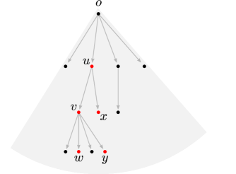
Figure 1: A possible configuration for $A_{t}$ when $G$ is a Galton-Watson tree. Vertices of $A_{t}$ are represented by dots: red if they belong to $R_{t}$ and black otherwise. Here $H_{t}=3$, given by the red paths $(u,v,w)$ and $(u,v,y)$, whereas $M_{t}=5$, given by the red cluster of vertices $\{u,v,w,x,y\}$.

2.2 Related processes

A model that is related to the present setting was introduced in [FS22a], and consists of a first passage percolation (FPP) process with conversion rates. In particular, a FPP process starts at a reference vertex spreading at rate 1 through vacant vertices. (Say that this process is of type 1.) Each occupied vertex, independently, switches at rate $\rho>0$ to a second type of FPP (type 2) that spreads at rate $\lambda>0$ through vacant sites as well as sites occupied by type 1. In this model, type $j\in\{1,2\}$ survives when there are vertices of type $j$ at all times. [FS22a] shows that when the underlying graph is a regular tree then coexistence is possible, while if the graph is a lattice then type 1 always dies if $\lambda$ is larger than some (small) critical value; the conjecture is that for $\lambda$ sufficiently small, type 1 survives. One of the main differences between such model and FPPHE with recovery is the fact in the former the type-2 process can occupy vertices already reached by type 1, whereas in the present setting both $\text{FPP}_{1}$ and $\text{FPP}_{\lambda}$ can spread only through vertices that have not yet been reached by the process.

Another known model related to the present framework is the so-called contact process (cf. for example [Lig99] for a formal description). In such a process, a vertex hosting a particle is said to be infected (here this would correspond to a red vertex). Infected vertices can pass on the infection to their neighbors at some constant rate $\lambda>0$, each infected vertex recovers at rate $1$ and it can become infected again. FPPHE with recovery is, however, very different from the contact process, as a vertex goes from red (infected) to black (recovered), and it will stay so forever.

The latter feature reminds of another related model, the so-called SIR model, where vertices on the graph are “Susceptible” or “Infected” or “Recovered”. In the SIR model each infected vertex spreads the infection to its susceptible neighbors at a constant rate. When a vertex recovers it becomes immune to infection and it will be unable to spread the infection any further. We refer to [Het00] for a review on SIR. While [Het00] mainly focuses on the spread of SIR in finite graphs of large size $N$, there are also results in the case of infinite trees, for example see [BF21]. The classical SIR model starts with a positive density of infected vertices, whereas in FPPHE with recovery the infection starts from a unique vertex (the origin) and all other vertices are seen as “susceptible”. Furthermore, in FPPHE with recovery, a vertex can be infected by $\text{FPP}_{\lambda}$ process even if the vertex trying to pass the infection has already recovered. This occurs when a seed is activated, representing an important difference between the two models.

3 Analysis on the semi-line: a proof of Theorem 1.1

In this section the graph $G$ is the infinite semi-line, i.e., $V=\mathbb{N}^{\ast}$; we set the origin $o:=\{1\}$ and the set of edges $E:=\{(n,n+1),~{}n\geq 1\}$. To simplify the notation, for all $n\geq 2$ set

$$T_{n}:=T_{(n-1,n)}.$$

Since a cluster in $G$ is a path, then for all $t\geq 0$ we have $M_{t}=H_{t}$. The recovery rate $\gamma>0$ is arbitrary but fixed. Recall that for any set $X$ we denote its cardinality by $\#X$.

3.1 Analysis of the limsup

The goal of this subsection is to find a non-decreasing function $h:\mathbb{R}_{+}\rightarrow\mathbb{R}_{+}^{*}$ such that

$$\mathbb{P}\left(\limsup_{t\rightarrow+\infty}\frac{H_{t}}{h(t)}=1\right)=1.$$

We start with a lemma that will be useful several times.

Lemma 3.1.

We have that

$$\mathbb{P}\left(\lim_{n\rightarrow+\infty}\frac{\tau_{n}}{n}=1\right)=1\quad\text{ and }\quad\mathbb{P}\left(\lim_{t\rightarrow+\infty}\frac{\#A_{t}}{t}=1\right)=1.$$

Proof.

By definition of $\tau_{n}$ (cf. (2.1)) and since $G$ is the semi-line, then $\tau_{n}=\sum_{k=2}^{n}T_{k}$. Therefore, by the (strong) law of large numbers, we have that $\frac{\tau_{n}}{n}\to 1$ almost surely.

Next, observe that for all $t\geq\tau_{n}$ we have $\#A_{t}\geq n$. Therefore, when $t\to\infty$ one has $\#A_{t}\rightarrow\infty$ almost surely (since for all $n$, $\tau_{n}<\infty$ almost surely). Thus, $\frac{\tau_{\#A_{t}}}{\#A_{t}}\to 1$ and $\frac{\tau_{\#A_{t}+1}}{\tau_{\#A_{t}}}\to 1$ almost surely. Since for all $t\geq 0$ one has $\tau_{\#A_{t}}\leq t<\tau_{\#A_{t}+1}$, then, $\frac{\#A_{t}}{t}\to 1$ as claimed. ∎

Next, we introduce an auxiliary object, which we call the tail red cluster. Recall that $[\![a,b]\!]$ denotes the connected path going from vertex $a$ to vertex $b$ in $G$.

Definition 3.2.

For $n\geq 1$ let $\mathbf{T}_{n}$ denote the largest red cluster present at time $\tau_{n}$ which includes vertex $n$; we call $\mathbf{T}_{n}$ the tail red cluster at time $\tau_{n}$. Moreover, for any $n\geq 1$ let $\widehat{H}_{n}$ be its size, i.e.,

$$\widehat{H}_{n}:=\#\mathbf{T}_{n}=\max\{m\in[\![1,n]\!]:[\![n-m+1,n]\!]\subset R_{\tau_{n}}\}.$$

The following result shows that, typically, the largest red cluster is the tail red cluster.

Proposition 3.3.

Let $h:\mathbb{N}^{*}\rightarrow\mathbb{R}_{>0}$ be a non-decreasing function, then:

$$\limsup_{n\rightarrow+\infty}\frac{\widehat{H}_{n}}{h(n)}=\limsup_{t\rightarrow+\infty}\frac{H_{t}}{h(\#A_{t})},\quad\mathbb{P}\text{-almost surely.}$$ (3.1)

Proof.

We start by showing that, almost surely, $\limsup_{n}\frac{\widehat{H}_{n}}{h(n)}\leq\limsup_{t}\frac{H_{t}}{h(\#A_{t})}.$

By construction, the size of the tail red cluster is at most the size of the largest red cluster, that is, $\widehat{H}_{n}\leq H_{\tau_{n}}$, and by definition $\#A_{\tau_{n}}=n$. Moreover $\tau_{n}\rightarrow\infty$ by Lemma 3.1, hence

$$\limsup_{n\to+\infty}\frac{\widehat{H}_{n}}{h(n)}\leq\limsup_{n\to+\infty}\frac{H_{\tau_{n}}}{h(\#A_{\tau_{n}})}\leq\limsup_{t\to+\infty}\frac{H_{t}}{h(\#A_{t})}.$$

Now we proceed with the reverse inequality. Recall that $\mathbf{C}_{i}$ denotes the recovery time of vertex $i$. W.l.o.g. assume $\limsup_{t}\frac{H_{t}}{h(\#A_{t})}>0$, (otherwise the result is clear), and fix $\ell\in\left(0,\,\limsup_{t}\frac{H_{t}}{h(\#A_{t})}\right)$. Fix an arbitrary value $n_{0}\geq 1$ and define a time $t_{0}:=t_{0}(n_{0})$ so that

$$t_{0}:=\max_{i\in[\![1,n_{0}]\!]}(\tau_{i}+\mathbf{C}_{i}).$$

Almost surely $t_{0}<+\infty$ and by definition of $\limsup$, there is a time $\hat{t}\geq t_{0}$ so that

$$\frac{H_{\hat{t}}}{h(\#A_{\hat{t}})}\geq\ell.$$ (3.2)

Now let $N\in[\![1,\#A_{\hat{t}}]\!]$ denote the rightmost vertex of a red cluster with size $H_{\hat{t}}$. If the cluster is not unique, just pick one arbitrarily. Clearly, since $\hat{t}\geq t_{0}$, then $N\geq n_{0}$ by definition of $t_{0}$.

We now claim that $\widehat{H}_{N}\geq H_{\hat{t}}$ and $\hat{t}\geq\tau_{N}$ (see Figure 2). To see this, we reason as follows. Since $N\leq\#A_{\hat{t}}$, then by time $\hat{t}$ vertex $N$ must be already part of the aggregate, implying $\hat{t}\geq\tau_{N}$. Moreover, between times $\tau_{N}$ and $\hat{t}$ there might have been some recoveries in the cluster of size $\widehat{H}_{N}$, implying $\widehat{H}_{N}\geq H_{\hat{t}}$. Using the facts that $N\geq n_{0}$ and that both functions $h$ and $t\mapsto\#A_{t}$ are non-decreasing, we obtain

$$\widehat{H}_{N}\stackrel{{\scriptstyle\eqref{eq:Hhat}}}{{\geq}}\ell h(\#A_{\hat{t}})\ \stackrel{{\scriptstyle\hat{t}\geq\tau_{N}}}{{\geq}}\ \ell h(\#A_{\tau_{N}})=\ell h(N).$$

By putting everything together, we have that

$$\limsup_{n\to+\infty}\frac{\widehat{H}_{n}}{h(n)}\geq\ell,\quad\mathbb{P}\text{-almost surely}.$$

By letting $\ell\rightarrow\limsup_{t}\frac{H_{t}}{h(\#A_{t})}$ we obtain the claim. ∎

Figure 2: A representation of the reasoning behind the proof of Proposition 3.3; possible configuration for $A_{\hat{t}}$ and $A_{\tau_{N}}$ where $N$ is the rightmost vertex of a maximizing cluster for $H_{\hat{t}}$.

Remark 3.4.

On the right-hand side of (3.1), the denominator is not a deterministic function of $t$. However, we will be able to get rid of the randomness with the help of Lemma 3.1.

The next step is to find a non-decreasing function $h:\mathbb{N}^{*}\rightarrow\mathbb{R}_{>0}$ such that

$$\limsup_{n\rightarrow+\infty}\frac{\widehat{H}_{n}}{h(n)}=1,\quad\mathbb{P}\text{-almost surely}.$$

In order to do this, we will compute the distribution of $\widehat{H}_{n}$ for all $n\geq 1$.

Lemma 3.5.

Recall that $\gamma>0$ is the recovery rate of the red vertices. For all $n\geq 1$ and $m\in[\![0,n]\!]$,

$$\mathbb{P}(\widehat{H}_{n}\geq m)=\left[\prod_{k=1}^{m-1}(1+k\gamma)\right]^{-1}.$$

Proof.

Observe that

$$\{\widehat{H}_{n}\geq m\}=\bigcap_{j=n-m+1}^{n}\left\{\mathbf{C}_{j}>\sum_{k=j+1}^{n}T_{k}\right\}.$$

Now we exploit independence of the recovery clocks $(\mathbf{C}_{k})_{k\geq 1}$ as well as independence between $(\mathbf{C}_{k})_{k\geq 1}$ and the passage times. This gives

$$\begin{split}\mathbb{P}(\widehat{H}_{n}\geq m)&=\mathbb{E}\left[\mathbb{P}(\widehat{H}_{n}\geq m~{}|~{}(T_{k})_{k\geq 1})\right]=\mathbb{E}\left[\prod_{j=n-m+1}^{n}\exp\left(-\gamma\sum_{k=j+1}^{m}T_{k}\right)\right]\\ &=\mathbb{E}\left[\exp\left(-\gamma\sum_{k=1}^{m-1}kT_{n-m+1+k}\right)\right]=\prod_{k=1}^{m-1}\int_{0}^{+\infty}e^{-k\gamma x}e^{-x}\mathrm{d}x=\left[\prod_{k=1}^{m-1}(1+k\gamma)\right]^{-1},\end{split}$$

as claimed. ∎

To simplify the notation, for all $m\geq 1$ set

$$\Pi(m):=\left[\prod_{k=1}^{m-1}(1+k\gamma)\right]^{-1}.$$

In the following, $\Gamma$ denotes the usual Gamma function and $\Gamma^{-1}$ its inverse. By its fundamental properties, for all $m\geq 0$ we have

$$\Pi(m)=\gamma^{-(m-1)}\frac{\Gamma(\gamma^{-1})}{\Gamma(m+\gamma^{-1})}.$$

We now show that $\Gamma^{-1}$ is a good candidate for the function $h$; for this result we need the following classical fact (which follows by Stirling’s approximation).

Fact 3.6.

Let $\delta>0$ be a fixed value. Then, as $x\to\infty$, we have $\frac{\Gamma(x+\delta)}{\Gamma(x)}\sim x^{\delta}$.

Theorem 3.7.

Almost surely, $\limsup_{n\rightarrow+\infty}\frac{\widehat{H}_{n}}{\Gamma^{-1}(n)}=1$.

Proof.

We start by showing that $\mathbb{P}\left[\limsup_{n}\frac{\widehat{H}_{n}}{\Gamma^{-1}(n)}>r\right]=0$, for all $r>1$. Consider any fixed value $r>1$ and for all $n\geq 1$ define

$$m_{n}:=\left\lceil r\Gamma^{-1}(n)\right\rceil.$$

Furthermore, for all $m\geq 0$ set

$$c_{m}:=\#\{j\geq 1~{}|~{}m=m_{j}\}.$$

Roughly speaking, $c_{m}$ represents the number of times such that $m$ appears as some $m_{n}$.

By Lemma 3.5 and collecting together equal terms in the sum we obtain

$$\sum_{n\geq 1}\mathbb{P}[\widehat{H}_{n}\geq r\Gamma^{-1}(n)]=\sum_{n\geq 1}\Pi(m_{n})\mathbf{1}_{m_{n}\leq n}\leq\sum_{m\geq 0}c_{m}\Pi(m).$$ (3.3)

Now observe that for all $m\geq 2r+1$ and $j\geq 1$, since $\Gamma$ is an increasing function, we have

$$m_{j}=m\iff m-1<r\Gamma^{-1}(j)\leq m\iff\Gamma\left(\frac{m-1}{r}\right)<j\leq\Gamma\left(\frac{m}{r}\right),$$

implying that $c_{m}\sim\Gamma\left(\frac{m}{r}\right)-\Gamma\left(\frac{m-1}{r}\right)$. Now, from Fact 3.6 we deduce that, as $m\to\infty$,

$$\frac{\Gamma\left(\frac{m}{r}\right)}{\Gamma\left(\frac{m-1}{r}\right)}\sim\left(\frac{m}{r}-\frac{1}{r}\right)^{1/r}\sim m^{1/r}\to\infty,$$

from which it follows that $c_{m}\sim\Gamma\left(m/r\right)$, as $m\rightarrow\infty$. Since $r>1$, Fact 3.6 and the ratio test imply that the series in (3.3) converges. In fact, as $m\to\infty$,

$$\frac{c_{m+1}\Pi(m+1)}{c_{m}\Pi(m)}\sim\frac{\Gamma\left[\frac{m+1}{r}\right]}{\Gamma\left[\frac{m}{r}\right]\gamma m}\sim\frac{m^{\frac{1}{r}-1}}{\gamma r^{\frac{1}{r}}}\rightarrow 0.$$

The first Borel-Cantelli lemma implies that almost surely only finitely many events of the sequence $(\{\widehat{H}_{n}\geq r\Gamma^{-1}(n)\})_{n\geq 1}$ will be realized. Since $r>1$ was arbitrary,

$$\mathbb{P}\left(\limsup_{n\to+\infty}\frac{\widehat{H}_{n}}{\Gamma^{-1}(n)}\leq 1\right)=1.$$

Now we show that $\mathbb{P}\left[\limsup_{n}\frac{\widehat{H}_{n}}{\Gamma^{-1}(n)}\geq r\right]=1$, for all $r<1$. Let $r\in(0,1)$ and fix $s\in(1,\frac{1}{r})$. Similarly to what we did in the first part, for all $n\geq 1$ define $k_{n}:=\lfloor n^{s}\rfloor$ and $w_{n}:=\left\lceil r\Gamma^{-1}(k_{n})\right\rceil$. Since for all $m$ large $\Gamma^{-1}(m)=o(\log(m))$, then by construction

$$\frac{w_{n+1}}{k_{n+1}-k_{n}}\sim\frac{r\Gamma^{-1}(n^{s})}{sn^{s-1}}\rightarrow 0\quad\text{as}\quad n\rightarrow+\infty.$$

For all large enough $n$, we also have $w_{n}\leq n$, hence there is $n_{0}\geq 1$ so that for all $n\geq n_{0}$ we have

$$w_{n}\leq n\quad\text{ and }\quad k_{n+1}-w_{n+1}>k_{n}.$$

By construction this implies that the events $(\{\widehat{H}_{k_{n}}\geq w_{n}\})_{n\geq n_{0}}$ are independent.

For all $m\geq 0$, denote $d_{m}:=\#\{j\geq n_{0}~{}|~{}m=w_{j}\}$ that is, the number of times that $m$ appears as a value $w_{n}$. Analogously to what done above, by lemma 3.5,

$$\sum_{n\geq n_{0}}\mathbb{P}(\widehat{H}_{k_{n}}\geq r\Gamma^{-1}(k_{n}))=\sum_{m\geq 0}d_{m}\Pi(m).$$ (3.4)

Finally, by reasoning as above gives $d_{m}\sim\Gamma(m/r)^{1/s}$ as $m\rightarrow\infty$. Thus, since $rs>1$, the series in (3.4) diverges. By the second Borel-Cantelli lemma, almost surely there is an infinite sub-sequence of events in $(\{\widehat{H}_{k_{n}}\geq w_{n}\})_{n\geq n_{0}}$ that will be realized, giving that $\mathbb{P}\left[\limsup_{n}\frac{\widehat{H}_{n}}{\Gamma^{-1}(n)}\geq r\right]=1$. Since $r\in(0,1)$ was arbitrary, the claim follows. ∎

Finally, we recall a classical result about the asymptotic behavior of $\Gamma^{-1}$ (which again follows by Stirling’s approximation), which will allow us to conclude the proof of the upper bound.

Fact 3.8.

As $t\rightarrow\infty$, $\Gamma^{-1}(t)\sim\frac{\log t}{\log\log t}$.

Finally we are ready to prove part (i) of Theorem 1.1.

Proof of Theorem 1.1(i).

It suffices to show that, almost surely,

$$\limsup_{t\rightarrow+\infty}\frac{H_{t}\log\log t}{\log t}=\limsup_{t\rightarrow+\infty}\frac{H_{t}}{\Gamma^{-1}(\#A_{t})}=1.$$

The second inequality is given by Theorem 3.7 and Proposition 3.3 since $\Gamma^{-1}$ is increasing. Finally, since $\#A_{t}\sim t$ almost surely by Lemma 3.1, the result follows from Fact 3.8. ∎

3.2 Analysis of the liminf

The goal of this subsection is to show that, almost surely, $\liminf_{t}H_{t}=0$. In order to do this, we need to introduce some notation.

Definition 3.9.

For all $n\geq 0$ and $v\in[\![1,n]\!]$, define the events

$$E_{v}^{n}:=\left\{\mathbf{C}_{v}>\sum_{k=v+1}^{n+1}T_{k}\right\},$$

namely, $E_{v}^{n}$ corresponds to the event that $v$ does not recover before the reaching time of vertex $n+1$. Moreover, define the complete recovery probability of order $n$ as the probability that all vertices in $[\![1,n]\!]$ have recovered before time $\tau_{n+1}$ i.e.,

$$\nu_{n}:=\mathbb{P}\left(\bigcap_{v=1}^{n}({E_{v}^{n}})^{c}\right)=1-\mathbb{P}\left[\bigcup_{v=1}^{n}{E_{v}^{n}}\right].$$

Recall the definition of $R_{t}$ from (2.2); then, $E_{v}^{n}=\{v\in R_{\tau_{n+1}}\}$. As a consequence, for all $n\geq 0$,

$$\nu_{n}=\mathbb{P}(R_{\tau_{n+1}}=\{n+1\}).$$

The next lemma gives a formula that will be used to obtain the asymptotic behavior of $(\nu_{n})_{n\geq 1}$.

Lemma 3.10.

For all $n\geq 1$ and $\ell\geq 1$, let

$$N_{\ell}^{n}:=\left\{\mathbf{x}\in({\mathbb{N}^{*}})^{\ell}:\sum_{k=1}^{\ell}\mathbf{x}_{k}\leq n\right\}\quad\text{and}\quad S_{\ell}(n):=\sum_{\mathbf{x}\in N_{\ell}^{n}}\prod_{k=1}^{\ell}(1+k\gamma)^{-\mathbf{x}_{k}}.$$

Then for all $n\geq 1$ we have

$$\nu_{n}=1+\sum_{\ell=1}^{n}(-1)^{\ell}S_{\ell}(n).$$ (3.5)

In words, $N_{\ell}^{n}$ is the set of all vectors of length $\ell$, so that the sum of the entries is at most $n$. $S_{\ell}(n)$ is a quantity related to the probability that all vertices in any set of cardinality $\ell\in\{1,2,\ldots,n\}$ recover before $\tau_{n+1}$. Its meaning will become clear in the proof.

Proof of Lemma 3.10.

Let $n\geq 1$, and for $k\in\{1,\ldots,n\}$ let $\mathcal{B}_{k}$ denote any subset of $[\![1,n]\!]$ of cardinality $k$; for $k=0$ set $\mathcal{B}_{0}:=\emptyset$. Then, by the inclusion-exclusion principle applied to $\mathbb{P}\left[\bigcup_{v=1}^{n}{E_{v}^{n}}\right]$,

$$\nu_{n}=1-\mathbb{P}\left[\bigcup_{v=1}^{n}{E_{v}^{n}}\right]=1-\sum_{k=1}^{n}(-1)^{k+1}\,\mathbb{P}\left[\bigcap_{v\in\mathcal{B}_{k}}E_{v}^{n}\right]=1+\sum_{k=1}^{n}(-1)^{k}\,\mathbb{P}\left[\bigcap_{v\in\mathcal{B}_{k}}E_{v}^{n}\right].$$

For simplicity, we re-write the above as

$$\nu_{n}=1+\sum_{A\subset[\![1,n]\!],~{}A\neq\emptyset}(-1)^{\#A}\,\mathbb{P}\left[\bigcap_{v\in A}E_{v}^{n}\right].$$ (3.6)

Now fix any subset $A\subset[\![1,n]\!]$, define $\ell:=\#A\geq 1$ and let $(a_{i})_{i\in[\![1,\ell]\!]}$ denote the elements of $A$ in increasing order. (Note that $A$ is not necessarily connected.) For convenience, define $a_{\ell+1}:=n+1$.

For all $\ell\geq 1$ (and hence for all $A\subset[\![1,n]\!]$) fixed, we now compute $\mathbb{P}\left[\bigcap_{v\in A}E_{v}^{n}\right]$. Start by observing that by independence of the recovery clocks $\{\mathbf{C}_{j}\}_{j}$ we have

$$\mathbb{P}\left(\bigcap_{v\in A}E_{v}^{n}\mid\{T_{k}\}_{k}\right)=\prod_{j=1}^{\ell}\mathbb{P}\left(\mathbf{C}_{a_{j}}>\sum_{k=a_{j}+1}^{n+1}T_{k}\mid\{T_{k}\}_{k}\right)=\prod_{j=1}^{\ell}\exp\left(-\gamma\sum_{k=a_{j}+1}^{n+1}T_{k}\right).$$ (3.7)

Therefore,

$$\begin{split}\mathbb{P}\left[\bigcap_{v\in A}E_{v}^{n}\right]&=\mathbb{E}\left[\mathbb{P}\left(\bigcap_{v\in A}E_{v}^{n}\mid\{T_{k}\}_{k}\right)\right]\ \stackrel{{\scriptstyle\eqref{eq:aux-clocks}}}{{=}}\ \mathbb{E}\left[\prod_{j=1}^{\ell}\exp\left(-\gamma\sum_{k=a_{j}+1}^{n+1}T_{k}\right)\right]\\ &=\mathbb{E}\left[\exp\left(-\gamma\sum_{j=1}^{\ell}\Bigl{(}j\sum_{k=a_{j}+1}^{a_{j+1}}T_{k}\Bigr{)}\right)\right]=\prod_{j=1}^{\ell}\prod_{k=a_{j}+1}^{a_{j+1}}\int_{\mathbb{R}_{+}}e^{-\gamma jt}e^{-t}\mathrm{d}t,\end{split}$$

where the last equality follows from independence of the recovery clocks and of the passage times. By solving the integral one obtains

$$\mathbb{P}\left[\bigcap_{v\in A}E_{v}^{n}\right]=\prod_{j=1}^{\ell}(1+j\gamma)^{-(a_{j+1}-a_{j})}.$$ (3.8)

Next, we define a function $\mathbf{\Psi}_{\ell}$ from $N_{\ell}^{n}$ to the collection of all subsets of cardinality $\ell$ contained in $[\![1,n]\!]$ as follows. For any fixed $\mathbf{x}=(\mathbf{x}_{1},\ldots,\mathbf{x}_{\ell})\in N_{\ell}^{n}$ let

$$\mathbf{\Psi}_{\ell}(\mathbf{x}):=\left\{n+1-\mathbf{x}_{1},~{}n+1-\mathbf{x}_{1}-\mathbf{x}_{2},~{}\ldots,~{}n+1-\sum_{i=1}^{\ell}\mathbf{x}_{i}\right\}.$$

This defines a one-to-one correspondence. By construction, for all $\mathbf{x}\in N_{\ell}^{n}$ equation (3.8) gives

$$\mathbb{P}\left[\bigcap_{v\in\mathbf{\Psi}_{\ell}(\mathbf{x})}E_{v}^{n}\right]=\prod_{k=1}^{\ell}(1+k\gamma)^{-\mathbf{x}_{k}}.$$

Finally, since $\mathbf{\Psi}_{\ell}$ defines a one-to-one correspondence, we obtain (3.5) by replacing $A\subset[\![1,n]\!]$ by $\mathbf{\Psi}_{\ell}(\mathbf{x})$ in (3.6) for every $\ell\in[\![1,n]\!]$ and $\mathbf{x}\in N_{\ell}^{n}$. ∎

The next result shows that $(\nu_{n})_{n\geq 1}$ converges to a positive value, which we compute explicitly.

Proposition 3.11.

The sequence $(\nu_{n})_{n\geq 1}$ converges to $e^{-1/\gamma}$.

Proof.

Fix an arbitrary $\ell\geq 1$ and recall the definition of $S_{\ell}(n)$ from Lemma 3.10. Define

$$S_{\ell}^{\infty}:=\sum_{\mathbf{x}\in(\mathbb{N}^{*})^{\ell}}\prod_{k=1}^{\ell}(1+k\gamma)^{-\mathbf{x}_{k}}.$$

Then, since $S_{\ell}(n)$ is a series with positive terms, we have $S_{\ell}(n)\rightarrow S_{\ell}^{\infty}$ as $n\to\infty$. Observe that since every entry of $\mathbf{x}$ varies in $\mathbb{N}^{*}$, we have

$$\sum_{\mathbf{x}\in(\mathbb{N}^{*})^{\ell}}\prod_{k=1}^{\ell}(1+k\gamma)^{-\mathbf{x}_{k}}=\prod_{k=1}^{\ell}\sum_{j=1}^{+\infty}\left(\frac{1}{1+k\gamma}\right)^{j},$$

which gives that for all fixed $\ell\geq 1$, one has $S_{\ell}^{\infty}=\prod_{k=1}^{\ell}\frac{1}{k\gamma}=\frac{1}{\ell!\gamma^{\ell}}$.

Now note that for all fixed $n\geq 1$ and $\ell\geq 1$ we have $S_{\ell}(n)\leq S_{\ell}^{\infty}$ (which is summable, as $\sum_{\ell\geq 0}S_{\ell}^{\infty}=e^{1/\gamma}$) then, by Lemma 3.10 and the dominated convergence theorem with respect to the counting measure, we deduce that

$$\lim_{n\rightarrow\infty}\nu_{n}=\lim_{n\rightarrow\infty}\sum_{\ell\geq 0}(-1)^{\ell}S_{\ell}(n)=\sum_{\ell\geq 0}(-1)^{\ell}S_{\ell}^{\infty}=\sum_{\ell\geq 0}\frac{(-1/\gamma)^{\ell}}{\ell!}=e^{-1/\gamma},$$

as claimed. ∎

The result below is an intermediate step, as it gives a liminf over a sub-sequence of times, namely the random times $(\tau_{n})_{n\geq 1}$. Clearly, $\liminf_{n\rightarrow\infty}H_{\tau_{n}}\geq\liminf_{t\rightarrow\infty}H_{t}$.

Remark 3.12.

In the following proof we implicitly use the fact that this process starts with a red particle (and not with a black one, as in the original definition of FPPHE). In fact, the process started at a vertex $v$ has the same distribution (modulo a translation in space and time) as the original process. This avoids several technicalities without affecting the definition of the model, since a black particle can always be seen as a red particle that has already recovered.

Theorem 3.13.

We have $\mathbb{P}(\{R_{\tau_{n}}=\{n\}\},\text{ i.o.})=1$.

Proof.

A straightforward consequence of Proposition 3.11 and Fatou’s lemma is

$$\mathbb{P}\left(\limsup_{n\to+\infty}\,\{R_{\tau_{n}}=\{n\}\}\right)\geq\limsup_{n\to+\infty}\mathbb{P}(R_{\tau_{n}}=\{n\})=\lim_{n\to+\infty}\nu_{n}=e^{-1/\gamma}>0.$$ (3.9)

We shall use this fact to deduce the statement from the Kolmogorov 0-1 law. Now we condition on the event that for all $k\geq 1$, $T_{k+1}<+\infty$ and $\mathbf{C}_{k}<+\infty$ as well as $\tau_{n}\to+\infty$; since this occurs almost surely (cf. Lemma 3.1), it is not a real restriction. For all $m\geq 1$ let

$$\mathcal{T}_{m}:=\sigma\left((\mathbf{C}_{j})_{j\geq m},\,(T_{j+1})_{j\geq m}\right)\quad\text{and}\quad\mathcal{T}:=\bigcap_{m\geq 1}\mathcal{T}_{m}$$

denote the $\sigma$-algebra generated by all recovery clocks and passage times starting from vertex $m$ and the corresponding tail-$\sigma$-algebra, respectively. Then observe that for all $k\geq 1$ we have

$$\limsup_{n\to+\infty}\,\{R_{\tau_{n}}=\{n\}\}=\limsup_{n\to+\infty}\,\{R_{\tau_{n}}\setminus[\![1,k-1]\!]=\{n\}\}.$$ (3.10)

This follows from the fact that, for all fixed $k$, the first $k-1$ vertices will eventually recover. (Recall that we are working under the assumption that all recovery times are finite.) Formally, denoting

$$t_{0}:=\max_{i\in[\![1,k-1]\!]}(\tau_{i}+\mathbf{C}_{i}),$$

we have $\tau_{n}>t_{0}$ for all $n$ large enough since $t_{0}<+\infty$ and $\tau_{n}\to+\infty$. Therefore since by construction after time $t_{0}$ the first $k-1$ vertices are recovered, this implies that $R_{\tau_{n}}=R_{\tau_{n}}\setminus[\![1,k-1]\!]$ for all $n$ large enough, hence (3.10) follows.

Now, observe that the RHS of (3.10) is $\mathcal{T}_{k}$-measurable for all $k$. In fact, for all $n\geq k$ the set $R_{\tau_{n}}\setminus[\![1,k-1]\!]$ corresponds to the set of red vertices for the process started at $k$ when the occupied region reaches size $n-k+1$. This implies that the LHS of (3.10) is $\mathcal{T}$-measurable and therefore the result follows by Kolmogorov 0-1 law and (3.9). ∎

Finally we are ready to prove part (ii) of Theorem 1.1.

Proof of Theorem 1.1(ii).

Now we will show that, almost surely, $\liminf_{t\rightarrow\infty}H_{t}=0$. Start by observing that, by definition of the process and the properties of the exponential distribution,

$$\mathbb{P}(\exists\,v,w\in[\![1,n]\!]\ :\ \tau_{v}=\mathbf{C}_{w}+\tau_{w})=0.$$ (3.11)

Moreover, by Theorem 3.13 almost surely there is an infinite increasing sub-sequence of indices $(n_{k})_{k}$ for which $R_{\tau_{n_{k}}}=\{n_{k}\}$. Since the process takes place in continuous time, by (3.11) for each $k\geq 1$ there is a value $\varepsilon_{k}\in(0,1)$ so that $R_{\tau_{n_{k}}-\varepsilon_{k}}=\{n_{k}\}\setminus\{n_{k}\}=\emptyset$. (In fact, at time $\tau_{n_{k}}$ vertex $\{n_{k}\}$ is the only one to be red and thus, right before, no vertex can be red.) Hence the result. ∎

4 Supercritical Galton-Watson trees

In this section $G$ is a supercritical Galton-Watson tree and the recovery rate $\gamma>0$ is arbitrary. More precisely, let $\zeta$ denote a distribution on the non-negative integers and consider a random variable $B\sim\zeta$. For all $k\geq 0$, let $\zeta(k):=\mathbb{P}(B=k)$. We require that $\mathbb{E}B:=\sum_{k\geq 1}k\zeta(k)>1$. Then, we assume that $\zeta$ is the offspring distribution that characterizes $G$. We let $\mathcal{S}$ denote the event that $G$ is infinite. Furthermore, define

$$\mathbb{P}_{\mathcal{S}}(\cdot):=\mathbb{P}(\cdot\mid\mathcal{S}).$$

To simplify the notation, for all $v\in V$ let $v^{-}$ denote the predecessor of $v$ in the (unique) non-backtracking path from the root $o$ to $v$ and set $T_{v}:=T_{(v^{-},v)}$. We also define

$$\boldsymbol{\alpha}:=\mathbb{E}B-1.$$ (4.1)

See Figure 3 for a simulation of FPPHE with recovery on $G$.

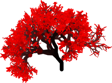
Figure 3: Simulation of $A_{t}$ with $B\sim\mathrm{Bin}(2,\frac{4}{5})$, $\gamma=\frac{1}{2}$ and $t=13$. Red dots are vertices of $R_{t}$ and dark lines are edges inside $A_{t}$.

Our next aim is to find two non-decreasing functions $h,g:\mathbb{R}_{\geq 0}\rightarrow\mathbb{R}_{>0}$ so that $\mathbb{P}_{\mathcal{S}}$-almost surely,

$$\liminf_{t\rightarrow+\infty}\frac{H_{t}}{h(t)}\geq 1\quad\text{and}\quad\liminf_{t\rightarrow+\infty}\frac{M_{t}}{g(t)}\geq 1.$$

4.1 Useful notation and properties

We start by defining two sequences of stopping times that will be widely used later on.

Definition 4.1.

For all $n\geq 1$, set $\theta_{n}:=\inf\{t\geq 0:\#A_{t}\geq n\}$. Moreover, for all $v\in V$, let $\tau_{v}:=\inf\{t>0\ :\ v\in A_{t}\}$.

Fix an integer $n\geq 1$ and assume $\#G\geq n$. Then $\theta_{n}$ is the reaching time of some vertex, and $\#A_{\theta_{n}}=n$. For any subset $A\subset V$ we define $\partial^{*}A$ to be its external boundary, i.e.,

$$\partial^{*}A:=\{w\in V\setminus A\ :\ \{v,w\}\in E,\text{ for some }v\in A\}.$$

In this subsection we provide asymptotic estimates for $\theta_{n}$ and $\#\partial^{*}A_{\theta_{n}}$ as $n\to\infty$. The following lemma gives a characterization for the distribution of $(\#\partial^{*}A_{\theta_{n}})_{n\geq 1}$. Recall that the offspring distribution $\zeta$ is described at the beginning of Section 4.

Lemma 4.2.

Consider a sequence $(D_{i})_{i\geq 1}$ of i.i.d. random variables distributed according to the offspring distribution $\zeta$ and define a new sequence of random variables $(J_{n})_{n\geq 0}$ inductively by setting $J_{0}:=1$, and for all $n\geq 0$

$$J_{n+1}:=J_{n}+(D_{n+1}-1)\mathbf{1}_{\{J_{n}>0\}}.$$

Then, we have that $(\#\partial^{*}A_{\theta_{n}})_{n\geq 1}$ is distributed as $(J_{n})_{n\geq 1}$.

Proof.

Observe that conditionally on all the passage times, $(A_{\theta_{n}})_{n\geq 1}$ is a deterministic exploration process of $G$. More precisely, we start at the origin and we consecutively discover, one at the time, vertices of the external boundary of the currently explored region. In particular, we have that for all $n\geq 1$,

$$\#\partial^{*}A_{\theta_{n+1}}-\#\partial^{*}A_{\theta_{n}}$$

is independent of $(\#\partial^{*}A_{\theta_{k}})_{1\leq k\leq n}$ and, on the event $\#\partial^{*}A_{\theta_{n}}>0$, has distribution $\zeta-1$. The result follows then by induction. ∎

Figure 4: Illustration of the step-by step construction in the proof of Lemma 4.2.

Lemma 4.3.

Recall the definition of $\boldsymbol{\alpha}$ from (4.1). Almost surely on $\mathcal{S}$, we have

$$\frac{\theta_{n}}{\log n}\to\frac{1}{\boldsymbol{\alpha}}\quad\text{ and }\quad\frac{\#\partial^{*}A_{\theta_{n}}}{n}\to\boldsymbol{\alpha}.$$

Proof.

The first statement follows directly by applying the methods in [AK67] (which are also deeply discussed in [AN72, Sections I.12 and III.9]). Now we can apply Lemma 4.2. Since the event $\{G$ is infinite$\}$ can be rewritten as $\{\forall n\geq 1,~{}\#\partial^{*}A_{\theta_{n}}>0\}$, by Lemma 4.2 it suffices to show that, conditional on $\mathcal{S}^{\prime}:=\{\forall n\geq 1,\,~{}J_{n}>0\}$, almost surely $\frac{J_{n}}{n}\to\boldsymbol{\alpha}$. In order to show this, observe that, on $\mathcal{S}^{\prime}$, we have $J_{n}=1+\sum_{k=1}^{n}(D_{k}-1)$. By the strong law of large numbers, almost surely on $\mathcal{S}^{\prime}$, we have $\frac{J_{n}}{n}\to\boldsymbol{\alpha}$, giving the second statement. ∎

Now we introduce a class of auxiliary processes coupled with the original one.

Definition 4.4.

Let $v\in V$. We define the process shifted by $v$ to be the translated process started at a new root, namely $v$. In particular, say that now $v\neq o$ is the root, then we discard the edge connecting $v$ to $v^{-}$ and consider only the connected component containing $v$. This guarantees that the distribution of the process does not change. All quantities in the new version will present a superscript $(v)$, however, the random variables associated to each edge (passage times) and to each vertex (recovery clocks) will not be changed. (E.g., $T_{v}^{(v)}\equiv T_{v}$.)

This procedure is well defined because the Galton-Watson tree is invariant (in a distributional sense) with respect to translation. Thus, Remark 3.12 ensures that the process started at any vertex $v$ at time $\tau_{v}$ has the same distribution as the original one. In any collection of vertices so that none of them is a prefix of any other, the corresponding shifted processes are all independent of one another and distributed as the original one.

Proposition 4.5.

There is a random set of vertices $U\subset V$ such that,

• $\mathbb{P}_{\mathcal{S}}$-almost surely we have $1<\#U<+\infty$ and $\#\left(V\setminus\bigcup_{v\in U}V^{(v)}\right)<\infty$.

• Under $\mathbb{P}_{\mathcal{S}}$ and conditional on $U$, $(V^{(v)})_{v\in U}$ is a collection of independent random sets distributed as $V$.

Proof.

Proof of (i). For any $v\in V$, consider the set of “sons” (i.e., direct descendants) of $v$ which are roots of infinite sub-trees in $G$, and denote it by $\mathbf{S}_{v}:=\{w\in\partial^{*}\{v\}:\#G^{(w)}=+\infty\}$.

First, observe that $\mathbb{P}_{\mathcal{S}}$-almost surely there exists a vertex $v\in G$ such that $\#\mathbf{S}_{v}>1$. (Under $\mathbb{P}_{\mathcal{S}}$, $\{v\in G:\mathbf{S}_{v}\geq 1\}$ is an almost surely infinite supercritical Galton-Watson tree.) Then, note that that if $u,v\in V$ have a common ancestor $a\notin\{u,v\}$ and they are such that $\#\mathbf{S}_{u}>1$ and $\#\mathbf{S}_{v}\geq 1$, then $\#\mathbf{S}_{a}>1$. It follows that there is a (random) vertex $\mathbf{w}\in V$ that, $\mathbb{P}_{\mathcal{S}}$-almost surely, is the unique vertex such that $\#\mathbf{S}_{\mathbf{w}}>1$ and $\#\left(V\setminus V^{(\mathbf{w})}\right)<\infty$. We set $U:=\mathbf{S}_{\mathbf{w}}$; see Figure 5.

Proof of (ii). The second item follows directly from the definition of $U$, since $\mathbf{S}_{\mathbf{w}}$ is a (finite) set of “siblings” (hence not descendants of one another), and from the distributional invariance of the Galton-Watson tree. ∎

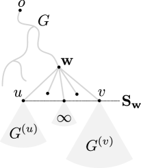
Figure 5: An illustration of the proof of Proposition 4.5.

4.2 Analysis of the liminf

In this subsection we shall prove results that will be applied to the sequences $(H_{t})_{t\in\mathbb{R}}$ and $(M_{t})_{t\in\mathbb{R}}$, hence write $(\mathcal{Q}_{t})_{t\in\mathbb{R}}$ to denote either of them. In the next subsection we shall see how to use this in order to prove Theorem 1.2. In a natural way, we set $\mathcal{Q}_{t}:=0$, for all $t<0$.

The first goal is to provide a sufficient property to characterize the asymptotic lower bound for $\mathcal{Q}_{t}$, as $t\to\infty$. More precisely, if $f:\mathbb{R}_{\geq 0}\rightarrow\mathbb{R}_{>0}$ is a non-decreasing function we want to get a non-trivial property on $f$ that guarantees $\liminf_{t}\frac{\mathcal{Q}_{t}}{f(t)}\geq 1$, $\mathbb{P}_{\mathcal{S}}$-almost surely.

In order to do so, we start by looking for an upper bound on $\mathbb{P}\left(\mathcal{Q}_{t}\leq m\right)$ when $(t,m)\in\mathbb{R}_{\geq 0}^{2}$ are large. We shall later apply the first Borel-Cantelli lemma to show that when $m=m(t)$ has the claimed expression, then the event $\{\mathcal{Q}_{t}\leq m\}$ occurs only finitely many times almost surely. Below we make use of the fact that a Galton-Watson tree is self-similar (in a distributional sense) and, when it survives, it grows exponentially fast. For all $(t,m,n)\in\mathbb{R}_{\geq 0}\times\mathbb{N}\times\mathbb{N}$ let

$$P_{m}^{n}(t):=\mathbb{P}[\mathcal{Q}_{t}\leq m,~{}\#\partial^{*}A_{t-1}\geq n].$$ (4.2)

Let $T\sim\mathrm{Exp}(1)$ be a random variable independent of the whole process. For all $m\in\mathbb{N}^{*}$ set

$$\eta(m):=\mathbb{P}[\mathcal{Q}_{1-T}\leq m].$$ (4.3)

Proposition 4.6.

For all$(t,m,n)\in\mathbb{R}_{\geq 0}\times\mathbb{N}\times\mathbb{N}$, we have

$$P_{m}^{n}(t)\leq\eta(m)^{n},$$

where $P_{m}^{n}(t)$ and $\eta(m)$ are defined in (4.2) and (4.3) respectively.

Proof.

By construction, for all fixed $t\geq 0$, the set $\partial^{*}A_{t-1}$ is almost surely finite. For all $n\geq 1$ let $\mathcal{B}_{n+}$ denote the set all possible shapes of size at least $n$ for $\partial^{*}A_{t-1}$, i.e. the set of all subsets of vertices $F$ such that $\#F\geq n$ and $\mathbb{P}(\partial^{*}A_{t-1}=F)>0$. Hence, by definition of $P_{m}^{n}(t)$ and of the shifted process, one has

$$\begin{split}P_{m}^{n}(t)&=\sum_{F\in\mathcal{B}_{n+}}\mathbb{P}(\{\mathcal{Q}_{t}\leq m\}\cap\{\partial^{*}A_{t-1}=F\})\\ &\leq\sum_{F\in\mathcal{B}_{n+}}\mathbb{P}[\{\forall v\in F,\,\mathcal{Q}_{t-\tau_{v}}^{(v)}\leq m\}\cap\{\partial^{*}A_{t-1}=F\}],\end{split}$$

where $\tau_{v}$ was introduced in Definition 4.1. Fix any $F\in\mathcal{B}_{n+}$. By the memoryless property of the exponential distribution, when we condition on $\{\partial^{*}A_{t-1}=F\}$, the set $(\tau_{v}-t+1)_{v\in F}$ is a collection of i.i.d. $\mathrm{Exp}(1)$ random variables.

Now consider the collection of processes shifted by $v$, where $v$ varies in $F$. Thus, conditional on $\{\partial^{*}A_{t-1}=F\}$, such collection consists of i.i.d. processes, distributed as the original one, independent of $(\tau_{v})_{v\in F}$. Therefore,

$$\mathbb{P}[\forall v\in F,\,\mathcal{Q}_{t-\tau_{v}}^{(v)}\leq m\mid F]=\left(\mathbb{P}[\mathcal{Q}_{1-T}\leq m]\right)^{\#F}$$

and hence

$$\begin{split}P_{m}^{n}(t)&\leq\sum_{F\in\mathcal{B}_{n+}}\left(\mathbb{P}[\mathcal{Q}_{1-T}\leq m]\right)^{\#F}\mathbb{P}(\partial^{*}A_{t-1}=F)=\eta(m)^{n}\left(\sum_{j\geq 0}\eta(m)^{j}\mathbb{P}(\#\partial^{*}A_{t-1}=n+j)\right).\end{split}$$

Since $\eta(m)\leq 1$ for all $m\geq 1$, then $\sum_{j\geq 0}\eta(m)^{j}\mathbb{P}(\#\partial^{*}A_{t-1}=n+j)\leq\mathbb{P}(\#\partial^{*}A_{t-1}\geq n)$. Hence the claim follows. ∎

An illustration of the reasoning in the above proof is given in Figure 6.

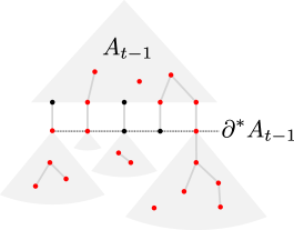
Figure 6: Possible configuration of the red vertices at time $t$.

The next auxiliary lemma gives a bound on the desired liminf restricted to a random sequence of times. Recall the definition of $\boldsymbol{\alpha}$ from (4.1).

Lemma 4.7.

Let $(Y_{n})_{n\geq 1}$ and $(Z_{n})_{n\geq 1}$ be two random sequences so that $(Z_{n})_{n\geq 1}$ is independent of the process with $\mathbb{P}(\frac{Y_{n}}{\log n}\to\boldsymbol{\alpha}^{-1})=1$ and $\mathbb{P}(\frac{Z_{n}}{\log n}\to\boldsymbol{\alpha}^{-1})=1$. Let $\eta(\cdot)$ be as in Proposition 4.6 and let $h:\mathbb{R}_{+}\rightarrow\mathbb{R}_{>0}$ be a non-decreasing function so that, for all $x>0$ large enough,

$$\eta\left(h(x)\right)\leq\exp(-1/x).$$ (4.4)

Then, for all $\beta\in(0,\boldsymbol{\alpha})$,

$$\liminf_{n\rightarrow+\infty}\frac{\mathcal{Q}_{Z_{n}}}{h(e^{\beta Y_{n}})}\geq 1,\quad\mathbb{P}_{\mathcal{S}}\text{-almost surely}.$$

Proof.

Fix $y\in(\frac{\beta}{\boldsymbol{\alpha}},1)$ and $z\in(y,1)$. For all $n\geq 1$ define

$$B_{n}:=\{\mathcal{Q}_{Z_{n}}\leq h(e^{\beta Y_{n}})\}\quad\text{ and }\quad G_{n}:=\{\#\partial^{*}A_{Z_{n}-1}\geq\beta n^{z},~{}h(e^{\beta Y_{n}})\leq h(n^{y})\}.$$

Since $\beta/\boldsymbol{\alpha}<y<z<1$, then from the assumption on the sequence $(Y_{n})_{n}$ we have that for $n$ large enough, $\beta Y_{n}<y\log n$, and hence $e^{\beta Y_{n}}<n^{y}$. Using this, together with the fact that $h$ is non-decreasing and that $(Z_{n})_{n\geq 1}$ is independent of the process, we deduce that for all $n\geq 1$,

$$\mathbb{P}(B_{n}\cap G_{n})\leq\mathbb{P}[\mathcal{Q}_{Z_{n}}\leq h(n^{y}),\ \#\partial^{*}A_{Z_{n}-1}\geq\beta n^{z}]=\mathbb{E}\left[P_{h(n^{y})}^{\beta n^{z}}(Z_{n})\right],$$

where the last equality follows from the definition in (4.2). Thus, by Proposition 4.6 and by assumption (4.4), for all $x$ large enough we get that for all $n\geq 1$ sufficiently large

$$\begin{split}\mathbb{P}(B_{n}\cap G_{n})&\leq\mathbb{E}\left[P_{h(n^{y})}^{\beta n^{z}}(Z_{n})\right]\ \stackrel{{\scriptstyle\text{Prop.\ \ref{prop_boundary_ineq}}}}{{\leq}}\mathbb{E}\left[\eta\left(h(n^{y})\right)^{\beta n^{z}}\right]\stackrel{{\scriptstyle\eqref{eq:assump-etah}}}{{\leq}}\exp\left(-\frac{1}{n^{y}}\,\beta n^{z}\right)=\exp(-\beta n^{z-y}).\end{split}$$

Since $z-y>0$, it follows that $\sum_{n\geq 1}\mathbb{P}(B_{n}\cap G_{n})<\infty$. Moreover, for all $E$ so that $\mathbb{P}(E)=0$ we also have $\mathbb{P}_{\mathcal{S}}(E)=0$. Thus, by the first Borel-Cantelli lemma

$$\mathbb{P}_{\mathcal{S}}\left[\limsup_{n\to+\infty}(B_{n}\cap G_{n})\right]=0.$$ (4.5)

Our next aim is to show that the sequence of events $(G_{n})_{n\geq 1}$ does not give any real contribution in the above intersection, implying that (4.5) only depends on the limsup of the events $(B_{n})_{n\geq 1}$.

Since $y/\beta>1/\boldsymbol{\alpha}$, from the asymptotic behavior of $(Y_{n})_{n\geq 1}$ it follows that almost surely for all $n\geq 1$ large enough we have $Y_{n}\leq\frac{y\log n}{\beta}$. Thus, since $h$ and the exponential function are non-decreasing,

$$h(e^{\beta Y_{n}})\leq h(n^{y}),\quad\mathbb{P}_{\mathcal{S}}\text{-almost surely}.$$ (4.6)

Using the assumption on the asymptotic behavior of $(Z_{n})_{n\geq 1}$ and the fact that $z<1$, together with Lemma 4.3, it follows that for all $n$ and $k$ large enough,

$$Z_{n}-1\geq\frac{\sqrt{z}}{\boldsymbol{\alpha}}\log n\quad\text{ and }\quad\theta_{k}\leq\frac{1}{\sqrt{z}\boldsymbol{\alpha}}\log k.$$

Thus, for all $n$ and $k$ large enough, $Z_{n}-1-\theta_{k}\geq\frac{\sqrt{z}}{\boldsymbol{\alpha}}\log n-\frac{1}{\sqrt{z}\boldsymbol{\alpha}}\log k$. Setting $k=\lfloor n^{z}\rfloor$,

$$Z_{n}-1\geq\theta_{\lfloor n^{z}\rfloor}\quad\mathbb{P}_{\mathcal{S}}\text{-almost surely, for all }n\text{ sufficiently large}.$$ (4.7)

Using again Lemma 4.3, since $\beta<\boldsymbol{\alpha}$, for all $n\geq 1$ large enough we have $\#\partial^{*}A_{\theta_{n}}\geq\beta(n+1)$, which implies that for all $n$ large and $t\geq\theta_{\lfloor n^{z}\rfloor}$ we have $\#\partial^{*}A_{t}\geq\beta n^{z}$. As a consequence, by (4.7) one obtains that there is a value $n_{0}$ so that, for all $n\geq n_{0}$,

$$\#\partial^{*}A_{Z_{n}-1}\geq n^{z},\quad\mathbb{P}_{\mathcal{S}}\text{-almost surely}.$$ (4.8)

Putting together equations (4.6) and (4.8) gives that there is a value $n_{1}$ so that, for all $n\geq n_{1}$, $G_{n}$ is realized. Together with (4.5) we obtain $\mathbb{P}_{\mathcal{S}}\left[\limsup_{n}B_{n}\right]=0$, which implies the claim. ∎

Finally, the previous lemma and Proposition 4.5 will be used to obtain a sufficient characterization for an asymptotic lower bound.

Theorem 4.8.

Let $h:\mathbb{R}_{+}\rightarrow\mathbb{R}_{+}^{*}$ be a non-decreasing function such that $\eta\left(h(x)\right)\leq\exp(-1/x)$ for all $x$ large enough. Then, for all $\beta\in(0,\boldsymbol{\alpha})$ we have

$$\liminf_{t\rightarrow+\infty}\frac{\mathcal{Q}_{t}}{h(e^{\beta t})}\geq 1,\quad\mathbb{P}_{\mathcal{S}}\text{-almost surely}.$$

Proof.

For all $t_{0}\geq 0$ define

$$\mathcal{Q}_{t_{0}}^{-}:=\lim_{t\to t_{0}^{-}}\mathcal{Q}_{t};$$

in words, $\mathcal{Q}_{t_{0}}^{-}$ coincides with $\mathcal{Q}_{t_{0}}$ except that it ignores the last vertex reached by the process at time $t_{0}$, if there is one. First we show that, for all $t>0$,

$$\mathcal{Q}_{t}\geq\mathcal{Q}_{\theta_{\#A_{t}+1}}^{-}\quad\text{and}\quad h(e^{\beta t})\leq h\left(e^{\beta\theta_{\#A_{t}+1}}\right)\quad\mathbb{P}_{\mathcal{S}}\text{-almost surely}.$$ (4.9)

The first inequality can be deduced from the following observations. At any fixed time $t$ the quantity $\mathcal{Q}_{\theta_{\#A_{t}+1}}^{-}$ is the size of a longest red path (or red cluster) at time $\theta_{\#A_{t}+1}$, excluding the last occupied vertex. Since $\theta_{\#A_{t}+1}$ is the first time that the occupied set has size $\#A_{t}+1$ then, when ignoring the last infected vertex, the occupied set has size $\#A_{t}$. Thus, $\theta_{\#A_{t}+1}\geq t$. However, between $t$ and $\theta_{\#A_{t}+1}$ only one vertex turns red (the one we ignore) while other red vertices might recover, then $\mathcal{Q}_{t}\geq\mathcal{Q}_{\theta_{\#A_{t}+1}}^{-}$. The second inequality follows from the fact that $\theta_{\#A_{t}+1}\geq t$ and $h$ is non-decreasing by assumption.

By dividing both terms of the first inequality in (4.9) by the terms in the second inequality and taking the $\liminf$, since $\#A_{t}\rightarrow\infty$, we obtain

$$\liminf_{t\rightarrow+\infty}\frac{\mathcal{Q}_{t}}{h(e^{\beta t})}\geq\liminf_{n\rightarrow+\infty}\frac{\mathcal{Q}_{\theta_{n}}^{-}}{h(e^{\beta\theta_{n}})}.$$

The sub-sequence of times $(\theta_{n})_{n}$ has some of the desired properties, but it is not independent of the process, thus we can not apply Lemma 4.7 directly. To get round this problem we apply Proposition 4.5. First, recall from Proposition 4.5 that $U$ is a discrete random variable representing a certain (finite) set of vertices. Therefore, it is enough to prove the claim on the event $\{U=F\}$ for any arbitrary finite set $F$, and then let $F$ vary. Fix a finite set of vertices $F$ such that $\mathbb{P}_{\mathcal{S}}(U=F)>0$, in particular we have $\#F>1$. From now on we reason under $\mathbb{P}_{\mathcal{S}}$ and conditional on the event $\{U=F\}$. For every $u\in F$, fix $u^{*}\in F$ such that $u^{*}\neq u$. For all $u\in F$ and $n\geq 1$, define

$$Y_{n}^{u}:=\tau_{u}+\theta_{n}^{(u)}\quad\text{and}\quad Z_{n}^{u}:=Y_{n}^{u}-\tau_{u^{*}}.$$

All but finitely many vertices of $V$ belong to $G^{(u)}$ for some $u\in F$. Thus, by Proposition 4.5, for all $n\geq 1$ large enough, for some $u\in F$ at time $\theta_{n}$ there will be a vertex $v$ in $G^{(u)}$ that will be reached by the process (see Figure 7). Therefore, $\mathbb{P}_{\mathcal{S}}$-almost surely given $\{U=F\}$ for all $n\geq 1$ big enough there exists a (random) vertex $\mathbf{v}_{n}\in F$ and a (random) index $L_{n}\geq 1$ such that

$$\theta_{n}=Y_{L_{n}}^{\mathbf{v}_{n}}.$$

By construction we have then

$$\mathcal{Q}_{\theta_{n}}^{-}\geq\mathcal{Q}^{(\mathbf{v}_{n}^{*})}_{Z_{L_{n}}^{\mathbf{v}_{n}}}.$$ (4.10)

In fact, start by noticing that, since $\theta_{n}=Y_{L_{n}}^{\mathbf{v}_{n}}$, then $Z_{L_{n}}^{\mathbf{v}_{n}}=Y_{L_{n}}^{\mathbf{v}_{n}}-\tau_{\mathbf{v}_{n}^{*}}=\theta_{n}-\tau_{\mathbf{v}_{n}^{*}}$ is the time elapsed from the moment vertex $\mathbf{v}_{n}^{*}$ has been reached by the process. Thus, the quantity $Q^{(\mathbf{v}_{n}^{*})}_{Z_{L_{n}}^{\mathbf{v}_{n}}}=Q^{(\mathbf{v}_{n}^{*})}_{Y_{L_{n}}^{\mathbf{v}_{n}}-\tau_{\mathbf{v}_{n}^{*}}}$ is the size of a maximal red path (or maximal red cluster) at time $\theta_{n}$ when we restrict the observed process to $G^{(\mathbf{v}_{n}^{*})}$. However, the size of a maximal red path (or red cluster) in this case is at least the size of a maximal red path (or red cluster) at time $\theta_{n}$ in $G$. Thus,

$$\mathcal{Q}_{\theta_{n}}\geq\mathcal{Q}^{(\mathbf{v}_{n}^{*})}_{Z_{L_{n}}^{\mathbf{v}_{n}}}.$$

Furthermore, the “minus” in the notation of (4.10) comes from the fact that at time $\theta_{n}$ only one vertex has been added to the cluster, and it was $\mathbf{v}_{n}\notin G^{(\mathbf{v}_{n}^{*})}$, hence we can ignore the last added vertex, obtaining (4.10). Now observe that, by definition, $L_{n}\rightarrow\infty$ as $n\rightarrow\infty$. Therefore,

$$\liminf_{n\rightarrow+\infty}\frac{\mathcal{Q}_{\theta_{n}}^{-}}{h(e^{\beta\theta_{n}})}\geq\min_{u\in F}\liminf_{n\rightarrow+\infty}\frac{\mathcal{Q}^{(u^{*})}_{Z_{n}^{u}}}{h(e^{\beta Y_{n}^{u}})},\quad\mathbb{P}_{\mathcal{S}}\text{-almost surely, given }\{U=F\}.$$

Next, fix $u\in F$. By Lemma 4.3, $\mathbb{P}_{\mathcal{S}}$-almost surely $\lim_{n}\frac{Z_{n}^{u}}{\log n}=\lim_{n}\frac{Y_{n}^{u}}{\log n}=\lim_{n}\frac{\theta_{n}^{(u)}}{\log n}=\frac{1}{\boldsymbol{\alpha}}$. Moreover, the shifted process corresponding to $u^{*}$ has the same distribution as the original one and it is independent of $(Z_{n}^{u})_{n\geq 1}$. Hence, by Lemma 4.7 we get

$$\liminf_{n\rightarrow+\infty}\frac{\mathcal{Q}^{(u^{*})}_{Z_{n}^{u}}}{h(e^{\beta Y_{n}^{u}})}\geq 1,\quad\mathbb{P}_{\mathcal{S}}\text{-almost surely, given }\{U=F\}.$$

By letting $F$ vary, we obtain the claim. ∎

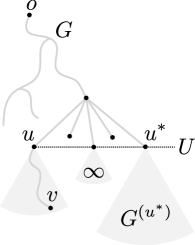
Figure 7: Illustration for the proof of Theorem 4.8.

4.3 Proofs of Theorem 1.2 and Corollary 1.3

In this subsection we use the previous results to compute the sought asymptotic lower bounds. The first two lemmas guarantee that the probabilities that we are investigating do indeed satisfy assumption (4.4). Recall that for all $t<0$ we set $H_{t}:=0$ and $M_{t}:=0$.

Lemma 4.9.

Let $T\sim\mathrm{Exp}(1)$ be independent of the process, and $r\in(0,1)$. Then for all $x>e$ large enough,

$$\mathbb{P}\left[H_{1-T}\leq\frac{r\log x}{\log\log x}\right]\leq e^{-1/x}.$$

Proof.

Fix $x>e$ and define

$$m_{x}:=\frac{r\log x}{\log\log x}\quad\text{and}\quad p_{x}:\mathbb{R}\rightarrow[0,1],~{}t\mapsto\mathbb{P}[H_{t}\leq m_{x}].$$ (4.11)

Next, denote

$$\mathcal{M}(x):=\inf\left\{1-p_{x}(t),~{}t\in\left[1-\log 2,1\right]\right\}.$$

By standard facts we have that

$$\mathbb{P}[H_{1-T}\leq m_{x}] =\mathbb{E}[p_{x}(1-T)\mathbf{1}_{T>\log 2}]+\mathbb{E}[p_{x}(1-T)\mathbf{1}_{T\leq\log 2}]$$

$$\leq\mathbb{P}(T>\log 2)+\mathbb{P}[T\leq\log 2]\sup_{t\in[1-\log 2,1]}p_{x}(t)=1-\frac{\mathcal{M}(x)}{2}.$$

Now, using the fact that $\log(1+z)\leq z$ for all $z>-1$, taking logarithms we obtain

$$\log\mathbb{P}[H_{1-T}\leq m_{x}]\leq\log\left(1-\frac{\mathcal{M}(x)}{2}\right)\leq-\frac{\mathcal{M}(x)}{2}.$$ (4.12)

Now, for all $n\geq 0$ we let the vertex $v_{n}$ correspond to the left-most individual of the $n$-th generation in the tree, and recall that $(\mathbf{C}_{v})_{v\in V}$ is the sequence of recovery clocks. Moreover, for all $v\in V$ let $B_{v}$ denote the number of children of vertex $v$. Set $T_{o}:=0$ for convenience and notice that, for all $t\in[1-\log 2,1]$,

$$\bigcap_{k=0}^{\lfloor m_{x}\rfloor}\left\{\mathbf{C}_{v_{k}}>1,~{}B_{v_{k}}\geq 1,~{}T_{v_{k}}<\frac{1-\log 2}{m_{x}+1}\right\}\subset\{H_{t}>m_{x}\}.$$

Therefore, considering the corresponding probabilities,

$$\mathcal{M}(x)\geq\mathbb{P}[B\geq 1]^{m_{x}+1}e^{-\gamma(m_{x}+1)}\left(1-\exp\left[-\frac{1-\log 2}{m_{x}+1}\right]\right)^{m_{x}}.$$ (4.13)

For the remainder of this proof, let

$$\widehat{\mathcal{M}}(x):=\mathbb{P}[B\geq 1]^{m_{x}+1}e^{-\gamma(m_{x}+1)}\left(1-\exp\left[-\frac{1-\log 2}{m_{x}+1}\right]\right)^{m_{x}}.$$ (4.14)

Next, since $\log(1-e^{-z})\sim\log z$ as $z\rightarrow 0^{+}$ together with (4.11), we have

$$\log\widehat{\mathcal{M}}(x)\sim m_{x}\log\left(\frac{1-\log 2}{m_{x}+1}\right)\sim-m_{x}\log m_{x}\sim-r\log x\quad\text{as}\quad x\rightarrow+\infty.$$

Thus, since $r<1$ we have that for all $x$ large enough

$$\widehat{\mathcal{M}}(x)\geq 2\exp(-\log x).$$

Finally, since $\widehat{\mathcal{M}}(x)\leq\mathcal{M}(x)$ (by (4.14) and (4.13)), by plugging this inequality into (4.12) we get

$$\begin{split}\log\mathbb{P}[H_{1-T}\leq m_{x}]\leq-\frac{\mathcal{M}(x)}{2}\leq-\frac{\widehat{\mathcal{M}}(x)}{2}\leq-\frac{1}{2}\,\frac{2}{x}=-\frac{1}{x}.\end{split}$$

By taking exponentials, we obtain the claimed result. ∎

Lemma 4.10.

Let $T\sim\mathrm{Exp}(1)$ be independent of the process and $r\in(0,1)$. Then for all $x>e^{e}$ large enough we have

$$\mathbb{P}\left[M_{1-T}\leq\frac{r\log x}{\log\log\log x}\right]\leq e^{-1/x}.$$

Proof.

We proceed as in the proof of Lemma 4.9. Fix $x>e^{e}$ and define

$$m_{x}^{\prime}:=\frac{r\log x}{\log\log\log x}\quad\text{and}\quad p_{x}^{\prime}:\mathbb{R}\rightarrow[0,1],\ t\mapsto\mathbb{P}[M_{t}>m_{x}].$$

Thus, by letting $\mathcal{M}^{\prime}(x):=\inf\left\{p_{x}^{\prime}(t),~{}t\in\left[1-\log 2,1\right]\right\}$, we have $\log\mathbb{P}[M_{1-T}\leq m_{x}]\leq-\mathcal{M}^{\prime}(x)/2$.

Let $\mathcal{V}_{x}$ denote the set of vertices corresponding to the first $1+\lfloor m_{x}^{\prime}\rfloor$ individuals of the (deterministic) binary tree. Now, since $G$ is supercritical, we can reason as follows. As in the previous proof, for $v\in V$ let $B_{v}$ denote the number of children of $v$. The probability that $G$ contains $\mathcal{V}_{x}$ is positive and, since the variables $\{B_{v}\}_{v}$ are i.i.d., it can be bounded by

$$\mathbb{P}\left[\bigcap_{v\in\mathcal{V}_{x}}\{B_{v}\geq 2\}\right]=(1-\zeta(0)-\zeta(1))^{1+\lfloor m_{x}^{\prime}\rfloor},$$

where, as defined at the beginning of Section 4, $\zeta(k)=\mathbb{P}(B_{v}=k)$. Furthermore, by definition of $\mathcal{V}_{x}$, we have that all such individuals are to be found within generation $\log_{2}(1+\lfloor m_{x}^{\prime}\rfloor)$.

Now set $T_{o}:=0$ for convenience. For all $t\in[1-\log 2,1]$, we have

$$\bigcap_{v\in\mathcal{V}_{x}}\left\{\mathbf{C}_{v}>1,~{}B_{v}\geq 2,~{}T_{v}<\frac{1-\log 2}{\log_{2}(m_{x}^{\prime}+1)}\right\}\subset\{M_{t}>m^{\prime}_{x}\}.$$

Therefore computing the probability,

$$\mathcal{M}^{\prime}(x)\geq\mathbb{P}[B_{o}\geq 2]^{m_{x}^{\prime}+1}e^{-\gamma(m_{x}^{\prime}+1)}\left(1-\exp\left[-\frac{1-\log 2}{\log_{2}(m_{x}^{\prime}+1)}\right]\right)^{m_{x}^{\prime}}=:\widehat{\mathcal{M}}^{\prime}(x).$$

Next, by reasoning like in the previous lemma, we obtain (for all fixed $r<1$)

$$\log\widehat{\mathcal{M}}^{\prime}(x)\sim-m_{x}^{\prime}\log\log m_{x}^{\prime}\sim-r\log x\quad\text{as}\quad x\rightarrow+\infty,$$

which implies the claim. ∎

Now we finally able to provide a proof of Theorem 1.2.

Proof of Theorem 1.2.

It suffices to show that, almost surely on $\mathcal{S}$,

$$\liminf_{t\rightarrow+\infty}\frac{H_{t}\log t}{t}\geq\boldsymbol{\alpha}\quad\text{and}\quad\liminf_{t\rightarrow+\infty}\frac{M_{t}\log\log t}{t}\geq\boldsymbol{\alpha}.$$

We start with the first claim. Fix $r\in(0,1)$ and for all $x\in(e,\infty)$ define $h(x):=\frac{r\log x}{\log\log x}$. This function is non-decreasing and by Lemma 4.9, it satisfies the assumptions of Theorem 4.8 for $(\mathcal{Q}_{t})_{t\in\mathbb{R}}\equiv(H_{t})_{t\in\mathbb{R}}$ and thus for all $\beta\in(0,\boldsymbol{\alpha})$ we have

$$\liminf_{t\to+\infty}\frac{H_{t}}{h(e^{\beta t})}\geq 1,\quad\mathbb{P}_{\mathcal{S}}\text{-almost surely}.$$

Simplifying the above expression we get $\liminf_{t}\frac{H_{t}\log t}{t}\geq r\beta$, $\mathbb{P}_{\mathcal{S}}$-almost surely. Then, by letting $\beta\rightarrow\boldsymbol{\alpha}$ and $r\rightarrow 1$ we get the first part of the claim. The second part of the claim is obtained similarly, by using Lemma 4.10 and Theorem 4.8 with $h$ so that, for all $x\in(e^{e},\infty)$, $h(x)=\frac{r\log x}{\log\log\log x}$ and $(\mathcal{Q}_{t})_{t\in\mathbb{R}}\equiv(M_{t})_{t\in\mathbb{R}}$. ∎

Remark 4.11.

Observe that $\mathbb{P}_{\mathcal{S}}(\#A_{t}\rightarrow\infty)=1$, and thus by Lemma 4.3,

$$\theta_{\#A_{t}}\sim\frac{\log\#A_{t}}{\boldsymbol{\alpha}}\sim\frac{\log(\#A_{t}+1)}{\boldsymbol{\alpha}}\sim\theta_{\#A_{t}+1}.$$

Then, since for all $t>0$ we have $\theta_{\#A_{t}}\leq t\leq\theta_{\#A_{t}+1}$, we deduce that for all $t$ large enough,

$$\log\#A_{t}\sim\boldsymbol{\alpha}t,\quad\mathbb{P}_{\mathcal{S}}\text{-almost surely}.$$ (4.15)

Finally we can provide a proof of Corollary 1.3.

Proof of Corollary 1.3.

By Remark 4.11 and using Fact 3.8, when $t\to\infty$ we obtain

$$\Gamma^{-1}(\#A_{t})\sim\frac{\log(\#A_{t})}{\log\log(\#A_{t})}\stackrel{{\scriptstyle\eqref{eq:aux-logAt}}}{{\sim}}\frac{\boldsymbol{\alpha}t}{\log(\boldsymbol{\alpha}t)}\sim\frac{\boldsymbol{\alpha}t}{\log t},\quad\mathbb{P}_{\mathcal{S}}\text{-almost surely}.$$

Finally, the result follows from Theorem 1.2. ∎

5 Proof of Theorem 1.4

The first part of the claim follows from Remark 4.11. In fact, since for all $t\geq 0$ we have $M_{t}\leq\#A_{t}$, the asymptotic given in (4.15) implies that for all $\delta>0$, $\mathbb{P}_{\mathcal{S}}-$almost surely for all $t$ big enough

$$\log M_{t}\leq\left(\boldsymbol{\alpha}+\frac{\delta}{2}\right)t.$$

The following parts are restricted to the case when $G$ has bounded degree, hence we can make use of [CS21a, Lemma 2.4], that states that whenever $G$ has maximal degree $\Delta$ then the following occurs. Let $\mathbf{c}_{1}>0$ be a fixed constant. Let $\mathcal{B}_{x}(r)$ denote the ball (in the graph metric) of radius $r$ centered at $x$. Then there is a value $\mathbf{c}_{\text{out}}=\mathbf{c}_{\text{out}}(\Delta,\mathbf{c}_{1})>1$ so that for every $t\geq 0$,

$$\mathbb{P}\left(A_{t}\not\subseteq\mathcal{B}_{o}(\mathbf{c}_{\text{out}}t)\right)\leq e^{-\mathbf{c}_{1}t}.$$ (5.1)

The remaining part of the proof of Theorem 1.4 is split into Lemmas 5.1 and 5.2 below.

Lemma 5.1.

Suppose that $G$ has bounded degree. Then we have

$$\mathbb{P}\left(\limsup_{t\to+\infty}\bigl{\{}A_{t}\subseteq\mathcal{B}_{o}(\mathbf{c}_{\text{out}}(t+1))\bigr{\}}\right)=1,$$

and in particular for all $\gamma>0$, $\mathbb{P}\left(\limsup_{t}\frac{H_{t}}{t}\leq\mathbf{c}_{\text{out}}\right)=1.$

Proof.

To get the first part, we investigate what happens at integer times and then use the fact that $(A_{t})_{t\geq 0}$ is non-decreasing. Let $o$ denote the origin of $G$. From (5.1),

$$\sum_{n\geq 0}\mathbb{P}\left(A_{n}\not\subseteq\mathcal{B}_{o}(\mathbf{c}_{\text{out}}n)\right)\leq\sum_{n\geq 0}e^{-\mathbf{c}_{1}n}<+\infty.$$

Therefore, by the first Borel-Cantelli lemma, almost surely for all $n\in\mathbb{N}$ large enough we have $A_{n}\subseteq\mathcal{B}_{o}(\mathbf{c}_{\text{out}}n)$ and in particular for all $t\geq 0$ large enough we get

$$A_{t}\subset A_{\lceil t\rceil}\subset\mathcal{B}_{o}(\mathbf{c}_{\text{out}}\lceil t\rceil)\subset\mathcal{B}_{o}(\mathbf{c}_{\text{out}}(t+1)).$$

Finally since for all $t\geq 0$, $H_{t}$ cannot be larger than the maximal distance of any vertex in $A_{t}$ from the origin, we obtain the claimed result. ∎

Now, in the same setting as above, we shall show that for all fixed $\varepsilon>0$, if the recovery rate $\gamma$ is large enough, then asymptotically as $t\to\infty$ the volume of the largest red cluster at time $t$ is at most $\varepsilon t$. Recall that $\Delta$ denotes the maximal degree of $G$.

Lemma 5.2.

Fix $\varepsilon>0$ arbitrarily small. Then there is a critical value $\gamma_{c}=\gamma_{c}(\Delta,\varepsilon,\mathbf{c}_{1})$ so that for all $\gamma>\gamma_{c}$,

$$\mathbb{P}\left(\limsup_{t\to+\infty}\frac{M_{t}}{t}\leq\varepsilon\right)=1.$$

Proof.

In this proof we shall use a percolation argument. Since the maximal degree of $G$ is $\Delta$, then $G$ is a subgraph of the regular tree of degree $\Delta$. We denote by $\mathbb{T}_{\Delta}$ such a tree. Furthermore, for all $t\geq 0$ set

$$\mathbb{T}_{\Delta}(t):=\{x\in\mathbb{T}_{\Delta}\ :\ d(o,x)\leq\mathbf{c}_{\text{out}}(t+1)\},$$

i.e., the set of nodes of $\mathbb{T}_{\Delta}$ up to generation $\lfloor\mathbf{c}_{\text{out}}(t+1)\rfloor$.

Since the minimum of $\Delta$ independent Exp($1$) random variables is distributed as an Exp($\Delta$), for all $v\in V$ the probability that $v$ activates a seed at any of its neighbors before recovering is

$$\mathbb{P}\left(\mathbf{C}_{v}>\min_{w\in\partial^{*}\{v\}}T_{w}\right)\leq\frac{\Delta}{\gamma+\Delta},$$

where the minimum is taken over all vertices $w$ that are (direct) descendants of $v$. Now define

$$p(\gamma):=\frac{\Delta}{\gamma+\Delta},$$

and consider Bernoulli site percolation on $\mathbb{T}_{\Delta}$ of parameter $p(\gamma)$. Clearly, by taking $\gamma$ large enough, we can make $p(\gamma)$ as small as we wish. Let $\gamma$ be so large that we are in the sub-critical regime (i.e.  there is almost surely no infinite open cluster) and such that if we set

$$\kappa:=p(\gamma)\bigl{(}1-p(\gamma)\bigr{)}^{\Delta-1}\frac{\Delta^{\Delta}}{(\Delta-1)^{\Delta-1}},$$

then we have

$$\frac{\Delta\,\mathbf{c}_{\text{out}}}{\log_{\Delta}(1/\kappa)}\leq\varepsilon.$$ (5.2)

At this point, let $\mathcal{K}_{t}$ denote the size of largest open cluster containing a vertex of $\mathbb{T}_{\Delta}(t)$. Then the main tool towards the sought conclusion is [AC11, Theorem 2] which states that

$$\mathbb{P}\left(\frac{\mathcal{K}_{t}}{\lfloor\mathbf{c}_{\text{out}}(t+1)\rfloor}\to\frac{1}{\log_{\Delta}(1/\kappa)}\right)=1.$$ (5.3)

We now define a coupling between the above site percolation process and FPPHE with recovery as follows. Since the probability that any vertex of $G$ activates a seed at any of its neighbors is at most $p(\gamma)$, we can declare each vertex that does so to be open.

For $t\geq 0$, let $M^{\prime}_{t}$ denote the size of the largest red cluster in $A_{t}\setminus\partial A_{t}$, where $\partial A_{t}$ denotes the internal boundary of $A_{t}$ (i.e., all $v\in A_{t}$ that have a neighbor outside $A_{t}$). Since the degree of $G$ is at most $\Delta$, one has $M_{t}\leq\Delta M^{\prime}_{t}+1$. The “+1” is needed if $M^{\prime}_{t}=0$. In fact, it might happen that red vertices are only present on $\partial A_{t}$, since they would be isolated red vertices, the largest red cluster has cardinality $1$. Moreover, since $\mathcal{B}_{o}(\mathbf{c}_{\text{out}}(t+1))\subseteq\mathbb{T}_{\Delta}(t)$, then by Lemma 5.1 we have that almost surely $A_{t}\subset\mathbb{T}_{\Delta}(t)$ for all $t$ large enough, thus $M^{\prime}_{t}\leq\mathcal{K}_{t}$ by construction of the coupling. Summing up, almost surely for all $t$ large enough, $M_{t}\leq\Delta\,\mathcal{K}_{t}+1$.

Finally, this implies the claim, as $\frac{\Delta\,\mathcal{K}_{t}+1}{t}\to\frac{\Delta\,\mathbf{c}_{\text{out}}}{\log_{\Delta}(1/\kappa)}\leq\varepsilon$ almost surely by (5.3) and (5.2). ∎

Acknowledgments.

E.C. acknowledges partial support by “INdAM–GNAMPA, Project code CUP$\_$ E53C22001930001”. This project started when T.G.S. was visiting the department of Mathematics and Physics at the University of Roma Tre for an internship, which was supported by the Erasmus+ program of the European Union and the Mathematics department of the ENS.

References

- [AC11] Ery Arias-Castro, Finite size percolation in regular trees, Statistics & Probability Letters 81 (2011), no. 2, 302–309.
- [AK67] Krishna B. Athreya and Samuel Karlin, Limit theorems for the split times of branching processes, Journal of Mathematics and Mechanics 17 (1967), no. 3, 257–277.
- [AN72] Krishna B. Athreya and Peter E. Ney, Branching processes, Die Grundlehren der mathematischen Wissenschaften, Band 196, Springer-Verlag, New York-Heidelberg, 1972. MR 373040
- [BF21] Christophe Besse and Grégory Faye, Spreading properties for sir models on homogeneous trees, Bulletin of Mathematical Biology 83 (2021).
- [CS21a] Elisabetta Candellero and Alexandre Stauffer, Coexistence of competing first passage percolation on hyperbolic graphs, Annales de l’Institut Henri Poincare (B) Probabilites et statistiques, vol. 57, Institut Henri Poincaré, 2021, pp. 2128–2164.
- [CS21b] , First passage percolation in hostile environment is not monotone, arXiv preprint arXiv:2110.05821 (2021).
- [Fin21] Thomas Finn, Topics in random growth models, 2021, Thesis (Ph.D.)–University of Bath.
- [FS22a] Thomas Finn and Alexandre Stauffer, Coexistence in competing first passage percolation with conversion, The Annals of Applied Probability 32 (2022), no. 6, 4459–4480.
- [FS22b] , Non-equilibrium multi-scale analysis and coexistence in competing first passage percolation, Journal of the European Mathematical Society (2022).
- [Het00] Herbert W. Hethcote, The mathematics of infectious diseases, SIAM Rev. 42 (2000), no. 4, 599–653. MR 1814049
- [Lig99] Thomas M. Liggett, Stochastic interacting systems: contact, voter and exclusion processes, Grundlehren der mathematischen Wissenschaften [Fundamental Principles of Mathematical Sciences], vol. 324, Springer-Verlag, Berlin, 1999. MR 1717346
- [SS19] Vladas Sidoravicius and Alexandre Stauffer, Multi-particle diffusion limited aggregation, Inventiones mathematicae 218 (2019), no. 2, 491–571.