Abstract

Thermal radiation becomes a prominent feature in the continuum spectrum of Venus longwards of $\sim$3 $\mu$m. The emission is traceable to the upper cloud and haze layers in the planet’s mesosphere. Venus’ thermal radiation spectrum is punctuated by CO₂ bands of various strengths probing into different atmospheric depths. It is thus possible to invert measured spectra of thermal radiation to infer atmospheric temperature profiles and offer some insight into the cloud and haze structure. In practice, the retrieval becomes complicated by the fact that the outgoing radiation is multiply scattered by the ubiquitous aerosol particles before leaving the atmosphere. We numerically investigate the radiative transfer problem of thermal radiation from the Venus night side between 3 and 5 $\mu$m with a purpose-built model of Venus’ mesosphere. Special emphasis is laid on the significance of scattering. The simulations explore the space of model parameters, which includes the atmospheric temperature, cloud opacity, and the aerosols’ size and chemical composition. We confirm that aerosol scattering must be taken into account in a prospective temperature retrieval, which means an additional complication to the already ill-posed retrieval problem. We briefly touch upon the degeneracy in the spectrum’s shape associated with parameterization of the Venus clouds. Reasonable perturbations in the chemical composition and size of aerosols do not significantly impact the model simulations. Although the experiments are specific to the technical characteristics of the Visual and Infrared Thermal Imaging Spectrometer on the Venus Express spacecraft, the conclusions are generally valid.

Kew words: thermal, radiation, Venus, scattering, mesosphere, temperature.

 

1 Introduction

The Venus mesosphere is a complex transition region that extends from $\sim$60 to $\sim$100 km above the planet’s surface. It vertically connects the domains of influence of the subsolar-to-antisolar and retrograde superrotating zonal flow patterns, each dominating the global wind dynamics above and below the mesosphere, respectively (Bougher et al.,, 2006). Further, the mesosphere is key to understand aspects of Venus such as the CO₂ and sulfur oxidation cycles (Mills and Allen,, 2007), the distribution of the unknown ultraviolet absorber (Titov et al.,, 2008), the deposition of solar energy (Crisp,, 1986), and the occurrence of the O₂ visible and near-infrared airglows (Crisp et al.,, 1996; García Muñoz et al.,, 2009).

The thermal radiation emerging from the planet’s night side provides a valuable window for remotely investigating the Venus mesosphere. Leaving aside the narrow features of thermal emission that occur at specific wavelengths below 2.3 $\mu$m (Allen and Crawford,, 1984; Carlson et al.,, 1991; Erard et al.,, 2009), Venus’ thermal radiation spectrum commences at $\sim$3 $\mu$m and peaks somewhere between 10 and 20 $\mu$m. The escaping photons originate from within the mesospheric upper cloud and haze layers, becoming absorbed and re-scattered in interactions with the aerosol particles. Absorption in a few CO₂ bands makes the thermal radiation spectrum amenable to investigation of the mesospheric thermal structure. The strong CO₂ bands at 4.3 and 15 $\mu$m are especially well-suited for the purpose, and provide a means for sounding the mesosphere from $\sim$100 km to $\sim$50–55 km with moderate-resolution spectroscopy (Carlson et al.,, 1991; Grassi et al.,, 2008; Roos-Serote et al.,, 1995; Zasova et al.,, 1999). Higher up, the atmosphere becomes too thin to leave an imprint on the spectrum, whereas lower down aerosol absorption prevents the photons from reaching the top of the atmosphere.

The Venus Express spacecraft of the European Space Agency was set into Venus orbit in 2006 (Svedhem et al.,, 2007). The Visual and Infrared Thermal Imaging Spectrometer (VIRTIS) (Drossart et al.,, 2007; Piccioni et al., 2007b, ) aboard Venus Express has since collected a few years worth of spectra. The instrument’s infrared channel covers the spectral range from 1 to 5 $\mu$m with a resolving power $\sim$200, which makes of the instrument a valuable tool for probing the thermal radiation spectrum near 4.3 $\mu$m. Another instrument on Venus Express, the Planetary Fourier Spectrometer (Formisano et al.,, 2006), was meant to probe both the 4.3 and 15 $\mu$m bands of CO₂ at high spectral resolution, but its unfortunate failure early in the mission impeded the task.

Recent work (Grassi et al.,, 2008; Irwin et al.,, 2008; Lee et al.,, 2012) has addressed various aspects of Venus’ thermal radiation spectrum shortwards of 5 $\mu$m related to VIRTIS observations. Although these studies explored the outgoing thermal radiation under a number of conditions, a systematic sensitivity analysis to the relevant parameters in the physical and numerical models has not yet been presented. Thus, the purpose of the current paper is to introduce a radiative transfer model (RTM) for simulating the thermal radiation from Venus’ night side between 3 and 5 $\mu$m, and demonstrate the model capacities with a number of examples that explore the problem’s sensitivity. Special attention is paid to the aerosol scattering of photons within the atmospheric medium as aerosols have the capacity of significantly modifying the spectrum of outgoing radiation. To our knowledge, only one prior work (Grassi et al.,, 2008) has addressed the details of multiple scattering for temperature retrievals in the Venus atmosphere. As noted by the authors, computational speed becomes a critical issue when the multiple-scattering treatment is required in line-by-line calculations.

The temperature retrieval problem in the Venus atmosphere differs from the usual treatment for Earth or Mars because multiple scattering is usually neglected in these two. By exploring the relevant space of model parameters, the paper intends to facilitate the interpretation of measured spectra and their sensitivity. Subsequent work will address the quantitative characterization and retrieval of temperatures and aerosol optical properties in the Venus atmosphere.

2 The forward model

The RTM solves the radiative transfer equation (RTE) for the atmosphere on a line-by-line basis. In a preliminary step, the RTM (optionally) produces two libraries of optical properties, one for the gases and one for the aerosols. Later, the RTM invokes the pre-calculated libraries as input into the RTE solver and outputs the synthetic spectrum. In its current version, the model uses DISORT as the RTE solver for multiple-scattering calculations (Stamnes et al.,, 1988, 2000). DISORT is a freely-available program for monochromatic radiative transfer calculations in plane-parallel stratified media that may include internal and external radiation sources. Because the interest of the paper lies in modeling Venus’ night side, we focus on the RTM’s capacity for treating thermal emission. In the calculation of the unscattered component of thermal radiation, we integrate the corresponding RTE along the line of sight with a routine built for the task.

The methodology for evaluating the gas and aerosol optical properties has largely been described elsewhere (García Muñoz and Pallé,, 2011; García Muñoz and Bramstedt,, 2012; García Muñoz and Mills,, 2012), so that only an overview is presented here. For the gas, we use the fundamental parameters for position, shape and strength of transition lines contained in the HITRAN 2008 database (Rothman et al.,, 2009). Line shapes are generally assumed to be of the Voigt type and approximated with simplified expressions (Schreier,, 1992). CO₂ lines are known to be sub-Lorentzian at distances of tens to hundreds of wavenumbers (Burch et al.,, 1969), a feature that is accounted for by a $\chi$($\nu$$-$$\nu_{0}$) function ($\leq$1) premultiplying the Voigt line shapes. In the RTM, we adopted the parameterization $\chi(\nu-\nu_{0})$=1 for $|\nu-\nu_{0}|$$\leq$$\nu_{\rm{min}}$, and =$\exp{(-a[|\nu-\nu_{0}|-\nu_{\rm{min}}]^{b})}$ otherwise, with $a$=0.08, $b$=0.8 and $\nu_{\rm{min}}$=5 cm^-1 (Winters,, 1964). The expression comes from a cell absorption experiment carried out at ambient temperature and pressures of up to 5 atm, and is specific to the blue side of the band. Later works investigated the red side of the band, and whether $\chi(\nu-\nu_{0})$ may also depend on temperature, pressure, or be asymmetric with respect to the band center $\nu_{0}$ (Burch et al.,, 1969; Le Doucen et al.,, 1985; Menoux et al.,, 1987; Perrin and Hartmann,, 1989). It is common, though, that the parameterization $\chi(\nu-\nu_{0})$ at shorter wavelengths must be slightly tuned to reproduce actual Venus spectra (Crisp,, 1986; Meadows and Crisp,, 1996).

CO is the only other gas that produces a noticeable signature at the relevant wavelengths. For the broadening of CO lines in CO₂, we corrected from the air-based parameters in HITRAN according to usual prescriptions (Bailey and Kedziora-Chudczer,, 2012). Rayleigh scattering by the CO₂ and N₂ background gases is considered, although its impact is minor with respect to aerosol scattering. The library of gas optical properties samples the pressure direction from 10 to 10^-8 bar with four levels for each ten-fold change in pressure, and the temperature direction with 27 temperature levels linearly spaced from 140 to 400 K. For pressures and temperatures in between, the gas optical properties are linearly interpolated.

In this study, five reference temperature profiles were considered, representative of average thermal conditions for latitudes of 30, 45, 60, 75 and 85^∘, and based on data obtained with a number of techniques by the Pioneer Venus Orbiter (PVO) and Venera missions (Seiff et al.,, 1985). The average PVO profiles have been confirmed by recent radio occultation measurements with the VeRa instrument on Venus Express (Tellmann et al.,, 2009). The profiles reveal that the temperature decays monotonically with altitude at the low latitudes, but that polewards the profiles develop a thermal inversion at 60–70 km altitude. The inversion is particularly pronounced in the so-called Venus’ cold collar, situated at latitudes of $\sim$70^∘, but reaches into the polar vortex. For a given temperature profile, the RTM converts from altitude to background pressure by integration of the hydrostatic balance equation.

The optical properties of the aerosols were calculated from Mie theory (Mishchenko MI,, 2002). The aerosol sizes were assumed to follow log-normal distributions described by their effective radius, $r_{\rm{eff}}$, and effective variance, $v_{\rm{eff}}$. In our reference implementation of aerosols, we considered only mode-2 particles with $r_{\rm{eff}}$ and $v_{\rm{eff}}$ values of 1.09 $\mu$m and 0.037, respectively, and a composition of H₂SO₄:H₂O in the ratio 84.5:15.5 by mass (Molaverdikhani et al.,, 2012). The adopted real and complex refractive indices are laboratory determinations at ambient temperature (Palmer and Williams,, 1975). The Mie calculations resulted in absorption and scattering cross sections and in coefficients of the Legendre polynomials for the scattering phase function over a set of wavelengths. At the non-tabulated wavelengths, the cross sections and Legendre polynomial coefficients were linearly and spline interpolated, respectively. For the implemented mode-2 aerosols, Fig. 1 shows (a) the extinction cross section and albedo, (b) the $g_{l}$ moments in the DISORT Legendre polynomial expansion for the scattering phase function, and (c) the scattering phase function against the scattering angle at a few wavelengths.

For simplicity, the RTM assumes that the aerosol number densities decay with altitude $z$ according to:

$$n_{\rm{aer}}(z)=\exp{(-(z-Z_{\rm{cloud}})/H_{\rm{aer}})}{\big{/}}{\sigma_{\lambda_{\star}}H_{\rm{aer}}},$$

where $Z_{\rm{cloud}}$ stands for the cloud top altitude, $H_{\rm{aer}}$ for the aerosol scale height, and $\sigma_{\lambda_{\star}}$= 4.5$\times$10^-8 cm² is a reference value for the aerosol extinction cross section at $\lambda_{\star}$=4 $\mu$m, see Fig. 1a. The given law satisfies $\tau_{\rm{nadir}}$=$\int_{Z_{\rm{cloud}}}^{\infty}\sigma_{\lambda_{\star}}n_{\rm{aer}}(z)dz$= 1, meaning that at 4 $\mu$m a nadir optical thickness of one is reached at $Z_{\rm{cloud}}$. More elaborate number density profiles are straightforward to implement. Given the complexity of the RT problem, though, the above formulation is deemed appropriate for the present purposes.

A major drawback of line-by-line approaches is the computational burden of solving the equations over a number of monochromatic bins that may often exceed several hundred thousand. Our full spectral grid samples the 1800–3500 cm^-1 interval of wavenumbers with 1.1$\times$10⁶ points spaced according to a geometric summation rule. The summation rule is built from the premise that the ratio $\Delta\nu_{i}/\nu_{i}$ of bin size and mid-wavenumber within the bin is constant. With bins $\Delta$$\nu$$\sim$(1–2)$\times$10^-3 cm^-1, this ensures at least two bins per Doppler width at the core of CO₂ lines throughout the mesosphere. However, a relaxation in the size of the spectral grid becomes acceptable when moderate spectral resolution is needed in the ultimate model spectrum. After some trials, we concluded that undersampling the full spectral grid led to negligible errors on the order of 1% in the model spectra at the VIRTIS resolution for undersampling factors of up to 50. Thus, the calculations presented here utilize a reduced grid that samples the 1800–3500 cm^-1 interval with only 2.2$\times$10⁴ points. After the line-by-line calculation, the spectra are convolved at the VIRTIS resolution onto a simpler spectral grid. For illustration, Fig. 2 shows model spectra for undersampling factors of 1, 10, 25 and 50. The corresponding curves are nearly indistinguishable.

As a check, we compared our CO₂ optical properties in a few conditions of temperature and pressure with those kindly provided to us by D. Grassi, finding an excellent agreement between the two sets. Also, we compared a model spectrum for an aerosol-free atmosphere as calculated by D. Grassi’s model and our model. Again, the agreement was excellent, even though the model radiance varied by orders of magnitude.

3 Exploring the outgoing thermal radiation spectrum

The thermal radiation predicted to emerge from the top of the atmosphere is affected by a number of parameters associated with both the numerical and physical models. Noting by y the model output, x the state vector of model parameters, and b an additional set of parameters from the numerical and physical models, the forward model F relates them through y= F(x, b) (Rodgers,, 2000). The distinction between x and b is subjective, and simply considers separately the parameters that one might attempt to infer from a model-observation comparison (x) and those that would remain fixed in the comparison (b).

In our formulation, y is the array of model radiances at the top of the atmosphere at selected wavelengths. Also, it will be convenient to consider that x=[$T_{0},T_{1},...,T_{l},...,T_{L}$, $H_{\rm{aer}}$, $Z_{\rm{cloud}}$] is a vector containing the temperatures $T_{l}$ at specified altitudes, and $H_{\rm{aer}}$ and $Z_{\rm{cloud}}$, the aerosol parameters introduced earlier. Array b contains parameters such as $r_{\rm{eff}}$, $v_{\rm{eff}}$ and the aerosol chemical composition in the physical model, and the number of streams up and down in the RTE solver for the numerical model.

To explore the impact of each parameter on the RTM’s output, the concept of weighting function (WF) plays a key role. The WF matrix is the matrix of partial derivatives $\partial\textbf{F(x, b)}/\partial\textbf{x}$ and expresses the output sensitivity to perturbations of the state vector about a given position. In the framework of the optimal estimation of atmospheric parameters (Rodgers,, 2000), accurate representations of the WF matrix are critical to speed up the convergence of the inversion algorithm and estimate the variance of the inferred parameters (Rodgers,, 2000). Next, we explore the structure of the WF matrix and assess our standard choice for b.

3.1 Reference spectra for the outgoing thermal radiation

Figure 3 shows on the left the model spectra for radiance (solid) and brightness temperature (dashed) for latitudes of 30, 45, 60, 75 and 85^∘. The brightness temperature $T_{\rm{B}}$ is the temperature of the equivalent black body that would produce the measured radiance. Panels on the right side show the respective profiles of atmospheric temperature. We adopted $H_{\rm{aer}}$=4 km in all the simulations, but implemented a different $Z_{\rm{cloud}}$ for each latitude. The prescribed $Z_{\rm{cloud}}$ values are based on Fig. 8a of a recent altimetry of the Venus clouds for average conditions at 1.6 $\mu$m (Ignatiev et al.,, 2009). In converting the cloud top altitude between the two wavelengths, it was estimated from the extinction cross section of Fig. 1a, that the clouds lie about 4 km lower at 4 $\mu$m than at 1.6 $\mu$m. The cloud top level is represented by a horizontal line in the temperature graphs. To highlight the contribution of multiple scattering, a second set of spectra (in red) was produced with the model’s scattering option turned off.

An inspection of the spectra from 4.3 to 5 $\mu$m shows general consistency with a similar exploration of the parameter space (Lee et al.,, 2012). The spectra reveal a number of features. Generally, $T_{\rm{B}}$ provides a more visual insight into the atmospheric temperature profiles than the radiance. For comparison with observations, though, $T_{\rm{B}}$ fails to give a direct measure of the photon counts, especially at the shorter wavelengths.

The $T_{\rm{B}}$ spectra for latitudes of 30 and 45^∘ show a mild bend near 3.5 $\mu$m (marked with the $\ast$ symbol in the top left panel of Fig. 3). This is the combined effect of the wavelength-dependent cross sections for mode-2 particles, see Fig. 1a, and the monotonic decrease in the atmospheric temperature profiles up to $\sim$90 km. Since the cross sections at 3 $\mu$m are smaller than at 3.5 $\mu$m, the spectrum at 3 $\mu$m shows radiance values from deeper in the atmosphere than at 3.5 $\mu$m. The bend is close to impossible to observe in the radiance spectra. By pointing it out, it becomes clear that the lack of significant structure in the aerosol cross sections introduces similarly insignificant changes to the spectra. This imposes a limitation to the capacity of models for inferring the aerosol opacity in the atmosphere over the 3–5 $\mu$m interval (Grassi et al.,, 2008). In this respect, the strong structure of the aerosol cross sections at 15 $\mu$m leads to a comparative advantage for investigating the aerosol distribution and temperature in the Venus atmosphere (Zasova et al.,, 1999).

Polewards of 45^∘, the adopted atmospheric temperature profiles exhibit inversions at 60–70 km (Tellmann et al.,, 2009). Focusing now on the spectrum for 75^∘ latitude, the shoulders of the 4.3-$\mu$m band (marked also with $\ast$ symbols in the second from the bottom left panel of Fig. 3) mimic to some extent the temperature profile in the inversion region. The reason for this is the rapidly-varying opacity of CO₂ at the edges of the band, that gives gradual access to most of the inversion layer. The shoulders can also be appreciated, with more difficulties, at 60 and 85^∘ latitude.

The comparison between the simulations with the full scattering treatment of the RTM and with the scattering option turned off are particularly revealing. Scattering enhances the outgoing radiance and therefore the inferred brightness temperature. The radiances calculated in multiple-scattering and non-scattering modes differ by up to a factor of $\sim$2, which translates into $T_{\rm{B}}$ differences of up to $\sim$15 K. This is to be expected because the single scattering albedo in the continuum is 0.4–0.5, and therefore a large fraction of emitted photons undergo various collisions before being totally absorbed. Typically, scattering seems to smooth out the spectra’s structure in the continuum. This is apparent in the 60 and 85^∘ latitude spectra near 4.3 $\mu$m, in which cases the shoulders of the CO₂ band nearly disappear. We tentatively attribute the effect to the weighting functions, broader in the multiple scattering case (see below), which mask the inversion layer by combining temperatures from a larger range of altitudes. Interestingly, inside the weaker CO₂ bands scattering leads to band depths that differ significantly from those obtained in the non-scattering mode. This is clearly seen at 4.7–4.8 $\mu$m because the combined gas-aerosol albedo remains high enough, and photons can scatter a few times before leaving the atmosphere.

3.2 The WF matrix for atmospheric temperature perturbations

Figure 4 shows WF matrices for perturbations in the temperature of the atmospheric layers, $T_{l}$. The matrices are displayed as $\partial T_{B}/\partial T_{l}$ to have them dimensionless. They were calculated by perturbing sequentially each $T_{l}$ by 10 K and finite-differencing the calculated brightness temperatures. Only the case for 75^∘ latitude is presented. The top and bottom panels show the calculations in the non- and multiple-scattering modes of the RTM.

Both WF matrices exhibit similar properties. In the nadir, the probed altitudes range from $\sim$100 km at the strongest absorption of the 4.3-$\mu$m band, to 56–57 km throughout most of the continuum. The latter is a little more than two scale heights below the prescribed $Z_{\rm{cloud}}$ level of 66 km at 4 $\mu$m. Both of the CO₂ bands at 4.8 and 5.1 $\mu$m leave distinct marks in the WF matrices. Generally, at each wavelength the WF can sense the atmosphere over a total vertical span of 3–4 scale heights. This can be better appreciated in Fig. 5, that shows the location of the maximum $\partial T_{B}/\partial T_{l}$ at each wavelength for the prescribed spectral resolution.

Figure 6 displays a few cuts of the WF matrix at selected wavelengths for the multiple-scattering (black) and non-scattering (red) calculations. This figure confirms some of the earlier ideas and shows clearly the range of altitudes probed throughout the spectrum. The weighting functions are notably narrower inside the strong 4.3-$\mu$m band than in the rest of the spectrum. Typically, sharp weighting functions facilitate the separation of contributions from different atmospheric altitudes. Multiple scattering broadens the weighting functions by $\sim$2–3 km. Physically, this can be explained by the longer path lengths of multiply-scattered photons.

3.3 The WF matrices for perturbations in the scale height and cloud top altitude

Figures 7 and 8 show the WF matrices of derivatives $\partial$$T_{B}$/$\partial$$H_{\rm{aer}}$ and $\partial$$T_{B}$/$\partial$$Z_{\rm{cloud}}$, respectively. They were calculated by finite differencing the brightness temperatures at a series of $H_{\rm{aer}}$ and $Z_{\rm{cloud}}$ values. The calculations are specific to 75^∘ latitude and take into account multiple scattering. For $H_{\rm{aer}}$=2–6 km and $Z_{\rm{cloud}}$=62–70 km, the structure of both WF matrices is remarkably similar, especially outside the strongest absorption bands. Their resemblance may contribute to the degeneracy of the temperature retrieval problem when both parameters are set independent in the retrieval algorithm (Grassi et al.,, 2008). Most of the details of the matrices can be understood in terms of the prescribed temperature profile, and from the fact that increasing either $H_{\rm{aer}}$ or $Z_{\rm{cloud}}$ tends to push upwards the atmospheric levels contributing to the outgoing radiance.

3.4 Sensitivity to other parameters

Our physical model for mode-2 particles assumes $r_{\rm{eff}}$=1.09 $\mu$m and $v_{\rm{eff}}$=0.037, and that the aerosols are liquid spherical droplets made of concentrated H₂SO₄ in H₂O at the 84.5 percent by mass. To further our exploration, we investigated different particle sizes and chemical compositions.

Typical values quoted for the percentage of H₂SO₄ in H₂O of the aerosols are in the range of 75–85% (Crisp,, 1986; Grinspoon et al.,, 1993; Hansen and Hovenier,, 1974). Figure 9 shows the radiances for our 75^∘ latitude atmosphere and percentage concentrations of 50, 75, 84.5 and 95.6. The results show that changes by reasonable amounts in the aerosol composition affect very moderately the spectra’s structure.

As with the chemical composition, there is some dispersion in the values reported in the literature for the aerosol size parameters, with $r_{\rm{eff}}$ being typically between 1 and 1.2 $\mu$m (Crisp,, 1986; Pollack et al.,, 1980). Also, recent works suggest that aerosols in the polar regions might be made of somewhat larger particles, which might point to differentiated cloud formation processes at low and high latitudes (Barstow et al.,, 2012; Lee et al.,, 2012; Wilson et al.,, 2008). Figure 9 shows our calculations with $r_{\rm{eff}}$=1.4 $\mu$m, an effective radius appropriate to the larger mode 2’ particles found in the middle clouds (Crisp,, 1986). The calculations show a mild sensitivity of the spectrum’s structure to the aerosol effective radius within accepted limits for the latter parameter.

Finally, we tested the impact of the number of streams in DISORT. The conclusion was that streams of four or more gave nearly identical results. Since the computational burden increases rapidly with the number of streams, we set the parameter to four.

4 The region from 4.5 to 4.8 $\mu$m

For conditions of low $Z_{\rm{cloud}}$, the synthetic spectra may exhibit a distinct feature near 4.6 $\mu$m. This can be appreciated in Fig. 10, that shows spectra for 75^∘ latitude and various cloud top altitudes. The feature resembles the thermal windows shortwards of 2.3 $\mu$m because, like them, it matches a local weakening in the CO₂ absorption spectrum. Unlike them, the feature at 4.6 $\mu$m originates in the mesosphere and not in the lower atmosphere below 50 km. Gas absorption in the affected spectral region is largely dominated by the far wings of the strong 4.3-$\mu$m band. Thus, the shape and intensity of the feature are affected by the parameterization $\chi(\nu-\nu_{0})$ for the CO₂ wings described earlier.

The impact on the feature at 4.6 $\mu$m of truncating $\chi(\nu-\nu_{0})$ at different distances from the line center can be seen in Fig. 11. The calculations were done with the 75^∘ latitude temperature profile but, to emphasize the absorbing properties of the CO₂ far wing, we set the cloud top at 62 km, somewhat lower than in the standard conditions. The figure shows also the result of taking $\chi(\nu-\nu_{0})$$\equiv$1 at all wavelengths, thus omitting the sub-Lorentzian shape of the CO₂ lines. It is apparent that long or unattenuated wings tend to annihilate the feature, and that adopting $\chi(\nu-\nu_{0})$$\equiv$1 alters the blue shoulder of the 4.3-$\mu$m band more than the red one. In relation with the latter remark, past works have noted the difficulty of reproducing the blue shoulder of Venus spectra (Grassi et al.,, 2008; Roos-Serote et al.,, 1995), which might require some tuning of the $\chi(\nu-\nu_{0})$ parameterization. A conclusive assessment of the optimal $\chi(\nu-\nu_{0})$ parameterization calls for the simultaneous determination of the temperature field, which is beyond the scope of the current paper.

The 4.5–4.8-$\mu$m region is also affected by the 0–1 fundamental band of CO. It is beyond the scope of the current paper to attempt the retrieval of CO abundances from VIRTIS/VEx thermal emission data, a task attempted in a recent work (Irwin et al.,, 2008). We will, though, comment briefly on the impact of multiple scattering on the CO spectral signature.

Figure 12 shows a few simulations of the spectrum from 4.5 to 4.8 $\mu$m with various amounts of CO. On this occasion, and to avoid the additional complication of the temperature inversion, we used the 30^∘ latitude temperature profile. We assumed a constant mixing ratio of CO throughout the mesosphere. The upper and lower sets of curves are the simulations for the multiple- and non-scattering problems, respectively. The conclusion to draw from the comparison is that the band depth is notably sensitive to whether the simulations are conducted in the multiple- or non-scattering modes of the RTM.

5 Some examples from VIRTIS

Figure 13 is a view of Venus’ Southern Pole at a few wavelengths between 3.83 and 5.1 $\mu$m obtained with VIRTIS in orbit #38 (2006/05/28, cube VI0038$\_$00.CAL). The images show the spatial structure of the South Polar vortex (Piccioni et al., 2007a, ). Figure 14 shows the corresponding thermal radiation and brightness temperature spectra at the indicated locations. Both representations give complementary insights into the Venus mesospheric structure. The locations were selected to give a broad perspective of thermal conditions and spatial variability in the near-pole region.

The maps at 3.83, 4.60 and 5.1 $\mu$m show a distinct elongated bright pattern, which is the manifestation of the polar vortex, with additional structure within. The level of detail in each monochromatic image depends on the actual depth being probed, see Fig. 5, and the signal-to-noise ratio of the data. The wavelengths of 4.41 and 4.52 $\mu$m, that fall within the main CO₂ absorption band, probe higher altitudes than the other wavelengths. For the latter two, the elongated pattern has (nearly) vanished. The level of detail of each image is mirrored in the corresponding spectra.

The spectra from the two points in the upper right corner of the images, outside the vortex, exhibit clear shoulders at the edges of the CO₂ band at 4.3 $\mu$m. Those shoulders are suggestive of a thermal inversion in the cold collar region. The feature at 4.6 $\mu$m, probably connected with clouds with relatively lower $Z_{\rm{cloud}}$ values, is apparent in a few spectra, specifically in those that probe the brightest regions in the images. Some related structure, see Fig. 10 for comparison, appears also at about 3.9 $\mu$m.

6 Summary and outlook

We presented a RTM for scattered thermal radiation in the Venus atmosphere from 3 to 5 $\mu$m. We explored the RTM’s sensitivity to a number of parameters in the physical and numerical model. The exercise demonstrated the potential importance of scattering in the upper cloud and haze layers over Venus’ mesospheric altitudes. In addition, it served to pinpoint potential difficulties that might occur in the eventual application of the RTM to inversion problems. Scattering is rarely represented in RTMs of planetary atmospheres in the thermal infrared. So, an investigation like this one should help clarify some of the differential characteristics of the propagation of thermal radiation in scattering atmospheres.

We are currently developing an inversion method to infer Venus’ mesospheric temperatures from VIRTIS spectra. The need to include multiple scattering means an additional difficulty because multiple-scattering RTE solvers consume significantly more resources than non-scattering RTE solvers. This is particularly true if the RTM must evaluate the WF matrix as part of the inversion algorithm. A linearized version of the RTM, such that it produces simultaneously both the radiance and the WF matrix, would be an interesting avenue to pursue.

Acknowledgements

AGM and PW acknowledge a postdoctoral fellowship from Gobierno Vasco. This work was supported by the Spanish MICIIN project AYA2009-10701 and AYA2012-36666 with FEDER support, Grupos Gobierno Vasco IT-464-07 and UPV/EHU UFI11/55. We gratefully acknowledge Davide Grassi for access to some of his model calculations.

Figure captions

Fig. 1.

Optical properties of assumed mode-2 particles, $r_{\rm{eff}}$=1.09 $\mu$m and $v_{\rm{eff}}$=0.037. (a) Extinction cross section and single scattering albedo. (b) DISORT-type $g_{l}$ coefficients for the Legendre polynomial expansion of the scattering phase function, with $l$ indicating the polynomial degree; $g_{1}$ is the classical asymmetry parameter. (c) The phase function against the scattering angle at selected wavelengths; the forward direction corresponds to a zero angle.

Fig. 2.

Model spectra of brightness temperature and radiance degraded at the VIRTIS resolving power. Each set of curves includes four different curves, calculated with undersampling factors (see text) of 1, 10, 25 and 50. Even at the largest undersampling (50, the value adopted for the subsequent model calculations), the accuracy loss is minor.

Fig. 3.

Left. Model spectra of brightness temperature (dashed) and radiance (solid) at the top of the atmosphere in down looking. Black and red curves are for multiple and non-scattering calculations, respectively. Right. At each reference latitude, atmospheric temperature profiles and levels of nadir optical opacity at 4 $\mu$m equal to one are shown.

Fig. 4.

WF matrix, $\partial$$T_{B}$/$\partial$$T_{l}$, for atmospheric temperature perturbations. Isoline contours with numbers indicated and drawn in a color code. The calculations are specific to the 75^∘ latitude temperature profile adopted. $Z_{\rm{cloud}}$=66 km at 4 $\mu$m. Top: Non-scattering. Bottom: Multiple scattering.

Fig. 5.

Wavelength dependence of the maxima in the WF matrix for atmospheric temperature perturbations in the multiple-scattering case from Fig. (4).

Fig. 6.

From Fig. 4, weighting functions $\partial$$T_{B}$/$\partial$$T_{l}$ at selected wavelengths. Black and red curves are for multiple and non-scattering calculations, respectively. For an easier visualization, the profiles were sequentially shifted by 0.15 K/K. From right to left, the wavelengths are 3.89, 3.93, 3.98, 4.03, 4.08, 4.13, 4.19, 4.24, 4.30, 4.36, 4.42, 4.48, 4.54, 4.61, 4.67, 4.74, 4.81, 4.88, and 4.96 $\mu$m.

Fig. 7.

WF matrix for perturbations in the scale height of aerosols, $\partial T_{B}/\partial H_{\rm{aer}}$, in the multiple-scattering mode of the RTM. Isoline contours indicated.

Fig. 8.

WF matrix for perturbations in the cloud top altitude, $\partial T_{B}/\partial Z_{\rm{cloud}}$, in the multiple-scattering mode of the RTM. Isoline contours indicated.

Fig. 9.

Spectra for 75^∘ latitude with alternative descriptions of the size and composition of mesospheric aerosols. Dashed line for brightness temperature, and solid line for radiance. Black: Curves for $r_{\rm{eff}}$=1.09 $\mu$m and compositions of 50, 75, 84.5 and 95.6 percent H₂SO₄ in H₂O. Red: Curve for $r_{\rm{eff}}$=1.4 $\mu$m and composition of 84.5 percent. Calculations in the multiple-scattering mode of the RTM.

Fig. 10.

Spectra for 75^∘ latitude, standard aerosol composition and size, multiple scattering, and various top cloud altitudes. The narrow feature at 4.6 $\mu$m is indicative of low $Z_{\rm{cloud}}$ values.

Fig. 11.

Spectra for 75^∘ latitude, $Z_{\rm{cloud}}$=62 km, and $\chi(\nu-\nu_{0})$ truncated at different distances or, alternatively, $\chi(\nu-\nu_{0})$$\equiv$1.

Fig. 12.

Spectra for 30^∘ latitude and various amounts of well-mixed CO. The top and bottom sets of curves are obtained in the multiple- and non-scattering modes of the RTM, respectively.

Fig. 13.

VIRTIS view of the Southern Pole in orbit #38. From top to bottom, wavelengths of 3.83, 4.41, 4.52, 4.60 and 5.1 $\mu$m.

Fig. 14.

VIRTIS spectra from the color-mark locations in Fig. 13. The dashed lines indicate the wavelengths (3.83, 4.41, 4.52, 4.60 and 5.1 $\mu$m ) in the monochromatic images of Fig. 13. The nature of the cold collar and the warm vortex is apparent in the structure of the black and green spectra, respectively.

Figures

Figure 1:

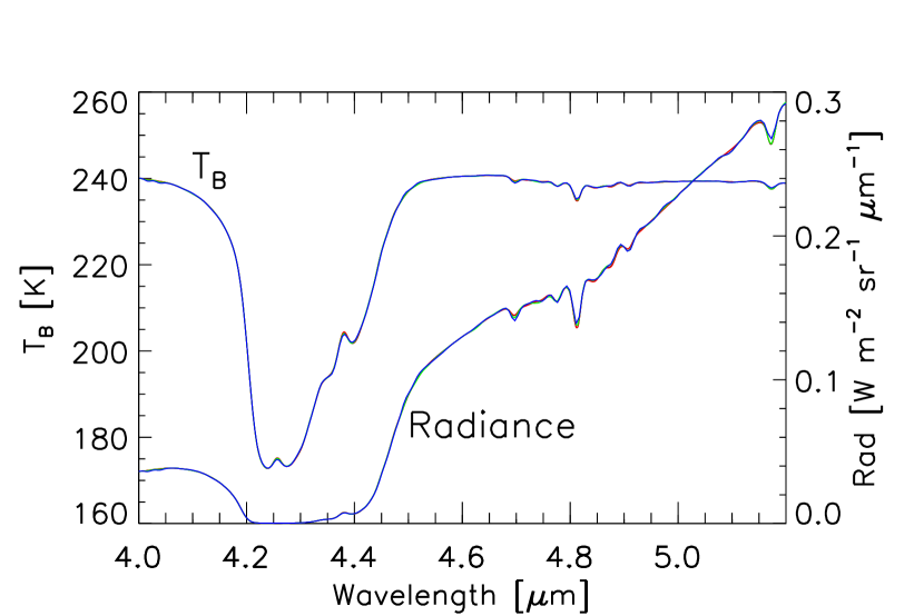
Figure 2:

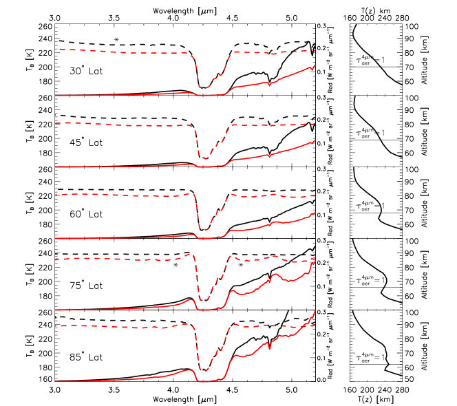
Figure 3:

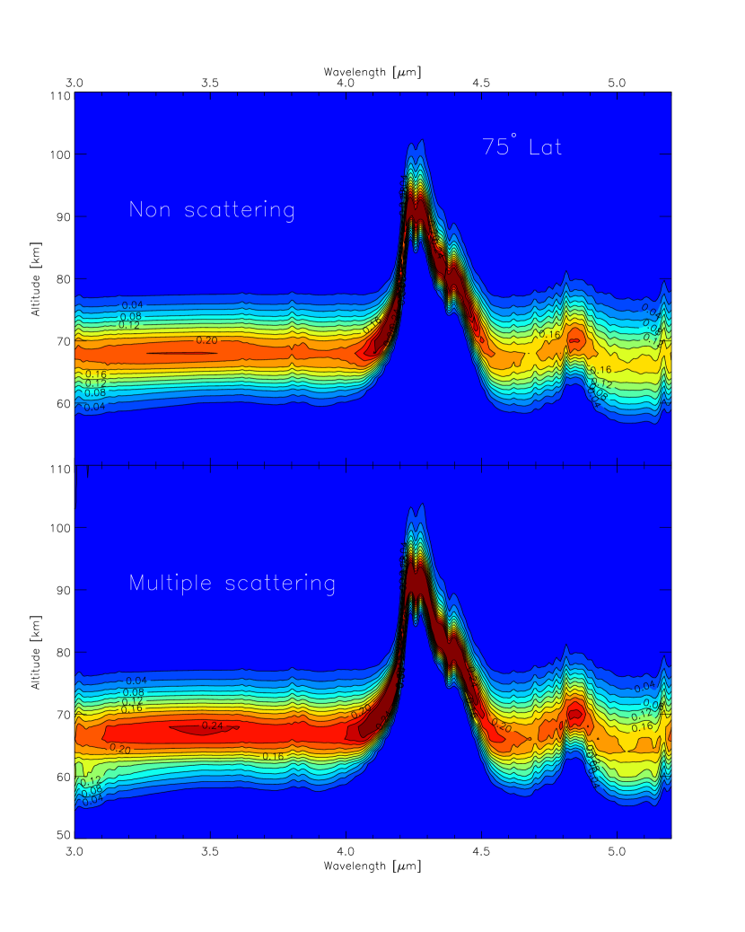
Figure 4:

Figure 5:

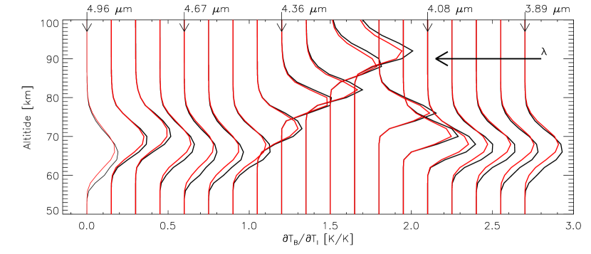
Figure 6:

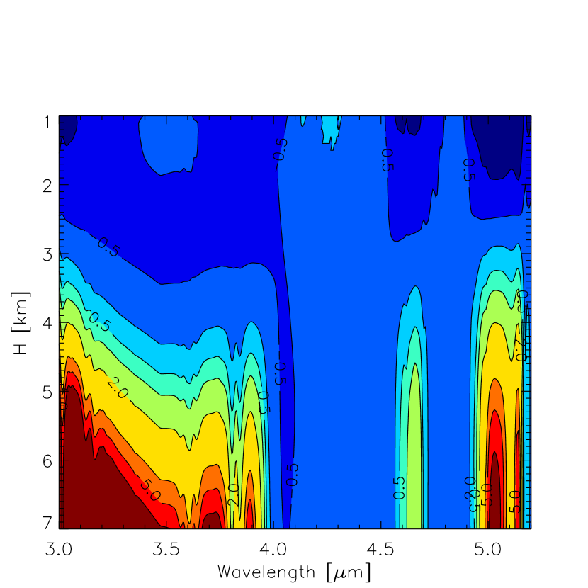
Figure 7:

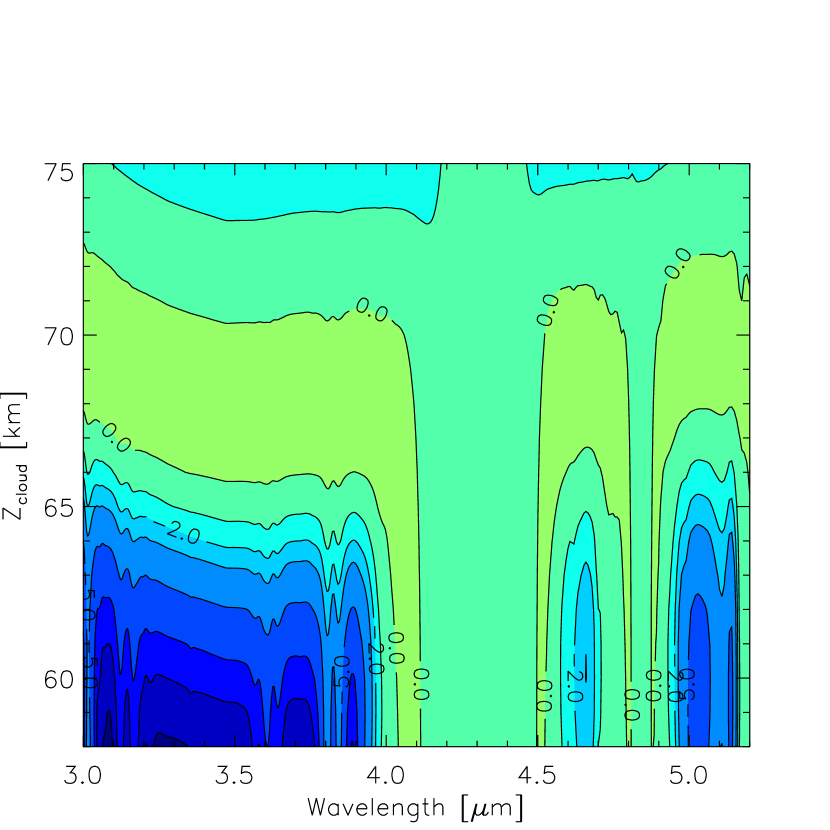
Figure 8:

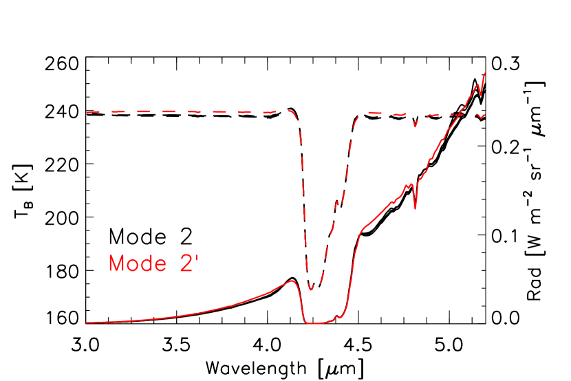
Figure 9:

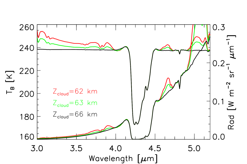
Figure 10:

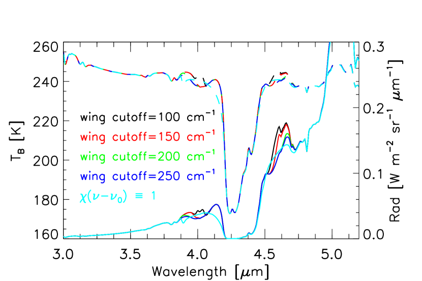
Figure 11:

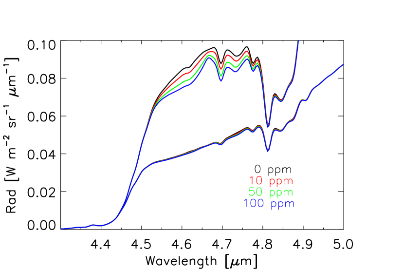
Figure 12:

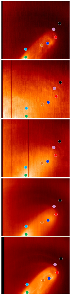
Figure 13:

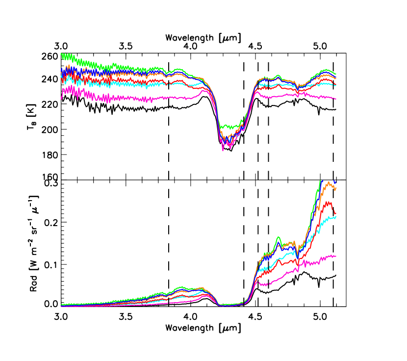
Figure 14:

References

- Allen and Crawford, (1984) Allen, D. A. and Crawford, J. W. (1984). Cloud structure on the dark side of Venus. Nature, 307:222–224.
- Bailey and Kedziora-Chudczer, (2012) Bailey, J. and Kedziora-Chudczer, L. (2012). Modelling the spectra of planets, brown dwarfs and stars using VSTAR. Mon. Not. R. Astron. Soc., 419:1913–1929.
- Barstow et al., (2012) Barstow, J. K., Tsang, C. C. C., Wilson, C. F., Irwin, P. G. J., Taylor, F. W., McGouldrick, K., Drossart, P., Piccioni, G., and Tellmann, S. (2012). Models of the global cloud structure on Venus derived from Venus Express observations. Icarus, 217:542–560.
- Bougher et al., (2006) Bougher, S. W., Rafkin, S., and Drossart, P. (2006). Dynamics of the Venus upper atmosphere: Outstanding problems and new constraints expected from Venus Express. Planet. Space Sci., 54:1371–1380.
- Burch et al., (1969) Burch, D. E., Gryvnak, D. A., Patty, R. R., and Bartky, C. E. (1969). Absorption of Infrared Radiant Energy by CO2 and H2O. IV. Shapes of Collision-Broadened CO2 Lines. J. Opt. Soc. Amer., 59:267–280.
- Carlson et al., (1991) Carlson, R. W., Baines, K. H., Kamp, L. W., Weissman, P. R., Smythe, W. D., Ocampo, A. C., Johnson, T. V., Matson, D. L., Pollack, J. B., and Grinspoon, D. (1991). Galileo infrared imaging spectroscopy measurements at Venus. Science, 253:1541–1548.
- Crisp, (1986) Crisp, D. (1986). Radiative forcing of the Venus mesosphere. I - Solar fluxes and heating rates. Icarus, 67:484–514.
- Crisp et al., (1996) Crisp, D., Meadows, V. S., Bézard, B., de Bergh, C., Maillard, J.-P., and Mills, F. P. (1996). Ground-based near-infrared observations of the Venus nightside: 1.27-m O2(ag) airglow from the upper atmosphere. J. Geophys. Res., 101:4577–4594.
- Drossart et al., (2007) Drossart, P., Piccioni, G., Adriani, A., Angrilli, F., Arnold, G., Baines, K. H., and 38 other authors (2007). Scientific goals for the observation of Venus by VIRTIS on ESA/Venus express mission. Planet. Space Sci., 55:1653–1672.
- Erard et al., (2009) Erard, S., Drossart, P., and Piccioni, G. (2009). Multivariate analysis of Visible and Infrared Thermal Imaging Spectrometer (VIRTIS) Venus Express nightside and limb observations. J. Geophys. Res. (Planets), 114:E00B27.
- Formisano et al., (2006) Formisano, V., Angrilli, F., Arnold, G., Atreya, S., Baines, K. H., and 45 other authors (2006). The planetary fourier spectrometer (PFS) onboard the European Venus Express mission. Planet. Space Sci., 54:1298–1314.
- García Muñoz and Bramstedt, (2012) García Muñoz, A. and Bramstedt, K. (2012). An investigation of the near-infrared collision induced absorption bands of oxygen with SCIAMACHY solar occultation data. JQSRT, 113:1566–1574.
- García Muñoz and Mills, (2012) García Muñoz, A. and Mills, F. P. (2012). The June 2012 transit of Venus. Framework for interpretation of observations. Astron. & Astrophys., 547:A22.
- García Muñoz et al., (2009) García Muñoz, A., Mills, F. P., Slanger, T. G., Piccioni, G., and Drossart, P. (2009). Visible and near-infrared nightglow of molecular oxygen in the atmosphere of Venus. J. Geophys. Res. (Planets), 114:12002.
- García Muñoz and Pallé, (2011) García Muñoz, A. and Pallé, E. (2011). Lunar eclipse theory revisited: Scattered sunlight in both the quiescent and the volcanically perturbed atmosphere. JQSRT, 112:1609–1621.
- Grassi et al., (2008) Grassi, D., Drossart, P., Piccioni, G., Ignatiev, N. I., Zasova, L. V., Adriani, A., Moriconi, M. L., Irwin, P. G. J., Negrão, A., and Migliorini, A. (2008). Retrieval of air temperature profiles in the Venusian mesosphere from VIRTIS-M data: Description and validation of algorithms. J. Geophys. Res. (Planets), 113:E00B09.
- Grinspoon et al., (1993) Grinspoon, D. H., Pollack, J. B., Sitton, B. R., Carlson, R. W., Kamp, L. W., Baines, K. H., Encrenaz, T., and Taylor, F. W. (1993). Probing Venus’s cloud structure with Galileo NIMS. Planet. Space Sci., 41:515–542.
- Hansen and Hovenier, (1974) Hansen, J. E. and Hovenier, J. W. (1974). Interpretation of the polarization of Venus. J. Atmos. Sci., 31:1137–1160.
- Ignatiev et al., (2009) Ignatiev, N. I., Titov, D. V., Piccioni, G., Drossart, P., Markiewicz, W. J., Cottini, V., Roatsch, T., Almeida, M., and Manoel, N. (2009). Altimetry of the Venus cloud tops from the Venus Express observations. J. Geophys. Res. (Planets), 114:E00B43.
- Irwin et al., (2008) Irwin, P. G. J., de Kok, R., Negrão, A., Tsang, C. C. C., Wilson, C. F., Drossart, P., Piccioni, G., Grassi, D., and Taylor, F. W. (2008). Spatial variability of carbon monoxide in Venus’ mesosphere from Venus Express/Visible and Infrared Thermal Imaging Spectrometer measurements. J. Geophys. Res. (Planets), 113:E00B01.
- Le Doucen et al., (1985) Le Doucen, R., Cousin, C., Boulet, C., and Henry, A. (1985). Temperature dependence of the absorption in the region beyond the 4.3-micron band head of CO2. I - Pure CO2 case. Appl. Opt., 24:897–906.
- Lee et al., (2012) Lee, Y. J., Titov, D. V., Tellmann, S., Piccialli, A., Ignatiev, N., Pätzold, M., Häusler, B., Piccioni, G., and Drossart, P. (2012). Vertical structure of the Venus cloud top from the VeRa and VIRTIS observations onboard Venus Express. Icarus, 217:599–609.
- Meadows and Crisp, (1996) Meadows, V. S. and Crisp, D. (1996). Ground-based near-infrared observations of the Venus nightside: The thermal structure and water abundance near the surface. J. Geophys. Res., 101:4595–4622.
- Menoux et al., (1987) Menoux, V., Le Doucen, R., and Boulet, C. (1987). Line shape in the low-frequency wing of self-broadened CO2 lines. Appl. Opt., 26:554–562.
- Mills and Allen, (2007) Mills, F. P. and Allen, M. (2007). A review of selected issues concerning the chemistry in Venus’ middle atmosphere. Planet. Space Sci., 55:1729–1740.
- Mishchenko MI, (2002) Mishchenko MI, Travis LD, L. A. (2002). Scattering, absorption and emission of light by small particles. Cambridge University Press, Cambridge.
- Molaverdikhani et al., (2012) Molaverdikhani, K., McGouldrick, K., and Esposito, L. W. (2012). The abundance and vertical distribution of the unknown ultraviolet absorber in the venusian atmosphere from analysis of Venus Monitoring Camera images. Icarus, 217:648–660.
- Palmer and Williams, (1975) Palmer, K. F. and Williams, D. (1975). Optical constants of sulfuric acid - Application to the clouds of Venus. Appl. Opt., 14:208–219.
- Perrin and Hartmann, (1989) Perrin, M. Y. and Hartmann, J. M. (1989). Temperature-dependent measurements and modeling of absorption by CO2-N2 mixtures in the far line-wings of the 4.3-micron CO2 band. JQSRT, 42:311–317.
- (30) Piccioni, G., Drossart, P., Sanchez-Lavega, A., Hueso, R., Taylor, F. W., and 100 other authors (2007a). South-polar features on Venus similar to those near the north pole. Nature, 450:637–640.
- (31) Piccioni, G., Drossart, P., Suetta, E., Cosi, M., Amannito, E., and 61 other authors, editors (2007b). VIRTIS: The Visible and Infrared Thermal Imaging Spectrometer, volume 1295 of ESA Special Publication.
- Pollack et al., (1980) Pollack, J. B., Toon, O. B., Whitten, R. C., Boese, R., Ragent, B., Tomasko, M., Eposito, L., Travis, L., and Wiedman, D. (1980). Distribution and source of the UV absorption in Venus’ atmosphere. J. Geophys. Res., 85:8141–8150.
- Rodgers, (2000) Rodgers, C. D. (2000). Inverse methods for atmospheric sounding. Theory and practice. World Scientific, Singapore.
- Roos-Serote et al., (1995) Roos-Serote, M., Drossart, P., Encrenaz, T., Lellouch, E., Carlson, R. W., Baines, K. H., Taylor, F. W., and Calcutt, S. B. (1995). The thermal structure and dynamics of the atmosphere of Venus between 70 and 90 KM from the Galileo-NIMS spectra. Icarus, 114:300–309.
- Rothman et al., (2009) Rothman, L. S., Gordon, I. E., Barbe, A., Benner, D. C., Bernath, P. F., and 38 other authors (2009). The HITRAN 2008 molecular spectroscopic database. JQSRT, 110:533–572.
- Schreier, (1992) Schreier, F. (1992). The Voigt and complex error function: A comparison of computational methods. JQSRT, 48:743–762.
- Seiff et al., (1985) Seiff, A., Schofield, J. T., Kliore, A. J., Taylor, F. W., and Limaye, S. S. (1985). Models of the structure of the atmosphere of Venus from the surface to 100 kilometers altitude. Adv. Space Res., 5:3–58.
- Stamnes et al., (1988) Stamnes, K., Tsay, S.-C., Jayaweera, K., and Wiscombe, W. (1988). Numerically stable algorithm for discrete-ordinate-method radiative transfer in multiple scattering and emitting layered media. Appl. Optics, 27:2502–2509.
- Stamnes et al., (2000) Stamnes, K., Tsay, S.-C., and Laszlo, I. (2000). DISORT, a general-purpose fortran program for discrete-ordinate-method radiative transfer in scattering and emitting layered media: Documentation of methodology, version 1.1.
- Svedhem et al., (2007) Svedhem, H., Titov, D. V., Taylor, F. W., and Witasse, O. (2007). Venus as a more Earth-like planet. Nature, 450:629–632.
- Tellmann et al., (2009) Tellmann, S., Pätzold, M., Häusler, B., Bird, M. K., and Tyler, G. L. (2009). Structure of the Venus neutral atmosphere as observed by the Radio Science experiment VeRa on Venus Express. J. Geophys. Res. (Planets), 114:E00B36.
- Titov et al., (2008) Titov, D. V., Taylor, F. W., Svedhem, H., Ignatiev, N. I., Markiewicz, W. J., Piccioni, G., and Drossart, P. (2008). Atmospheric structure and dynamics as the cause of ultraviolet markings in the clouds of Venus. Nature, 456:620–623.
- Wilson et al., (2008) Wilson, C. F., Guerlet, S., Irwin, P. G. J., Tsang, C. C. C., Taylor, F. W., Carlson, R. W., Drossart, P., and Piccioni, G. (2008). Evidence for anomalous cloud particles at the poles of Venus. J. Geophys. Res. (Planets), 113:E00B13.
- Winters, (1964) Winters, B. (1964). Line shape in the wing beyond the band head of the 4.3 band of CO2. JQSRT, 4:527–537.
- Zasova et al., (1999) Zasova, L. V., Khatountsev, I. A., Moroz, V. I., and Ignatiev, N. I. (1999). Structure of the Venus middle atmosphere: Venera 15 fourier spectrometry data revisited. Adv. Space Res., 23:1559–1568.