Network Analysis of U.S. Non-Fatal Opioid-Involved Overdose Journeys, 2018-2023

Abstract

We present a nation-wide network analysis of non-fatal opioid-involved overdose journeys in the United States. Leveraging a unique proprietary dataset of Emergency Medical Services incidents, we construct a journey-to-overdose geospatial network capturing nearly half a million opioid-involved overdose events spanning $2018$-$2023$. We analyze the structure and sociological profile of the nodes, which are counties or their equivalents, characterize the distribution of overdose journey lengths, and investigate changes in the journey network between 2018 and 2023. Our findings include that authority and hub nodes identified by the HITS algorithm tend to be located in urban areas and involved in overdose journeys with particularly long geographical distances.

Keywords: Opioid overdoses, Geospatial networks, Transportation networks, Public health, Emergency medical services, HITS algorithm

1 Introduction

The toll of the drug overdose epidemic in the United States is staggering; more than one hundred thousand people lost their life from a drug overdose in 2021 alone [1]. Opioids have been a major driver of the epidemic, and opioid overdose mortality in the U.S. has grown exponentially since $1979$ [2]. Furthermore, the rate of nonfatal drug overdose Emergency Medical Services (EMS) encounters involving opioids nearly doubled from January 2018 to March 2022 [3]. Evidence suggests that state-level efforts have been moderately successful in reducing misuse of prescription opioids [4], but such policies may have unintentionally increased opioid mortality by indirectly incentivizing illicit usage [5]. For every fatal drug overdose there are many more nonfatal overdoses, and EMS data uniquely provide information on where nonfatal overdoses occur, as well as details on patient residence. This information can be used for understanding how far from a person’s place of residence they experienced an overdose, hereafter called a journey to overdose.

Network analysis has been proven to be useful for studying multiple types of public health questions, including disease transmission, diffusion of health-related behavior and information, and social support networks, which are relevant to opioid overdose [6, 7, 8]. In the context of the opioid overdose crisis, social network analysis of Appalachians found that over half the individuals in their data set had a first-degree relationship with someone who experienced an opioid overdose, and this proportion was higher near city centers [9]. It was also found that measures of network centrality and prominence can elucidate illicit opioid-seeking behavior [10, 11].

To the best of our knowledge, Oser et al. applied the concept of geographical discordance to drug overdoses for the first time [12]. They found that people who use drugs who traveled to counties other than those of their residences for substance abuse treatment are more likely to relapse with prescription opioids. They also found that geographically discordant treatment efforts (i.e., when those in treatment obtain it in a county other than that of their residence) are more common among rural populations than suburban or urban ones. Johnson et al. studied trip distance to drug purchase arrest for several classes of controlled substances, leveraging arrest record data from Camden, New Jersey. They showed that race and ethnicity were significantly correlated with trip distance, underscoring the relationship between geospatial segregation and drug purchase patterns [13]. Forati et al. applied spatial network methods to analyze geographically discordant opioid overdoses, i.e., those that occur in locations distinct from the residence of the person who experienced the overdose. Their work, which concerned fatal incidents in Milwaukee, Wisconsin between 2017 and 2020, was the first to analyze an overdose journey network [14]. However, the trips quantified in these studies were relatively short, and the study included only a single locale. In the present study, we extend these works to a larger spatial scale (i.e., across counties) and to a time horizon that includes the COVID-19 pandemic.

2 Materials and methods

2.1 EMS Data

We utilize a proprietary dataset sourced from biospatial, Inc., a platform specializing in the collection and analysis of EMS data [15]. Company biospatial aggregates information from hundreds of counties across 42 states (currently 27 full-coverage states and 15 partial-coverage states). “Full coverage” states are those from which biospatial receives all records from the state EMS office, while “partial coverage” states provide a subset of the data, sometimes garnered through direct partnerships with EMS providers. Place-of-residence information is collected from the patient, patient’s history, or from the EMS destination (e.g., hospital). Data are available at the patient level, but exact information on overdose location and patient residence are not available due to privacy protections. We use aggregate information about overdose incident location and patient residence, derived from Federal Information Processing Standards (FIPS) codes, which identify counties or county equivalents (for simplicity, we also refer to them as counties in the following text) within the U.S.

To identify instances of opioid-involved overdoses in EMS records, we apply the Council of State and Territorial Epidemiologists (CSTE) Nonfatal Opioid Overdose Standard Guidance, which identifies suspected opioid-involved overdose encounters by querying coded data elements and patient care report narratives. Specifically, it considers provider impressions, symptoms observed, medications administered and the subsequent response, and keywords considered opioid-related or overdose-related. After sub-setting our data to nonfatal opioid occurrences, we then further remove request cancellations and EMS call-outs coded as assisting another primary agency [16].

Coverage and completeness of biospatial’s EMS data vary by time period and reporting agency. Therefore, our first exclusion criterion is counties without sufficient data, implemented by leveraging biospatial’s Underlying Event Coverage (UEC) metric, which compares the number of records submitted to biospatial and the number expected during a given time period for a county. The UEC uses probabilistic models of population characteristics and historical data. In this analysis, counties were included if they had a UEC of at least 75% during each quarter of the study period, following Casillas et al. [3]. Our second exclusion criteria includes counties that do not share Patient Care Report Narratives with biospatial, limiting the ability of the CSTE opioid overdose definition queries to identify encounters. Lastly, we excluded fatal opioid occurrences and focused on non-fatal opioid-involved overdose encounters.

2.2 Other data

We obtain demographic and socioeconomic statistics from the American Community Survey 2017-2021 5-Year Data Release (ACS). The ACS is an annual demographics survey managed by the U.S. Census Bureau, providing details on education, employment, housing, and more. The survey samples approximately 3.5 million addresses from across the U.S. annually [17].

We also use urbanicity data from the 2013 National Center for Health Statistics (NCHS) Urban–Rural Classification Scheme for Counties (URCS), which categorizes U.S. counties into the following six groups based on urbanization:

• Large central metro: counties that (i) are in a metropolitan statistical area (MSA) with at least one million residents, (ii) contain the entirety of the MSA’s largest principal city, and (iii) are exclusively populated within the MSA’s largest principal city or represent at least 250000 inhabitants in one of the MSA’s principal cities,

• Large fringe metro: counties in an MSA that have at least one million residents and are not classified as large central metro. These counties are, for example, the suburbs of large central metros,

• Medium metro: counties in an MSA with between $250000$ and $999999$ residents,

• Small metro: counties in an MSA with fewer than $250000$ residents,

• Micropolitan: counties in micropolitan statistical areas, and

• Noncore: counties in neither MSAs nor micropolitan statistical areas [18].

As in [3], we refer to large central metropolitan, large fringe metropolitan, medium metropolitan, or small metropolitan counties as being urban, and micropolitan and noncore counties as being rural, for simplicity. We also provide results for all six categories in Appendix A.3.

Finally, we extract geographic boundary coordinates from the U.S. Census 2000 Topologically Integrated Geographic Encoding and Referencing (TIGER) system [19]. The obtained data offer digital cartographic information for public use in the form of shape files.

2.3 Construction of a nationwide spatial network of overdose journeys

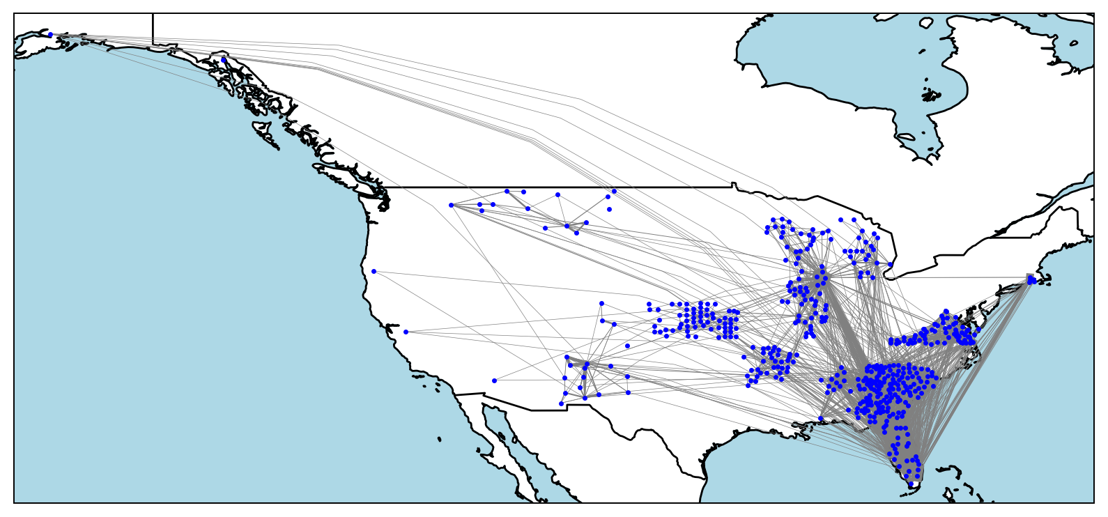
Figure 1: Visualization of the network of overdose journeys laid over a U.S. map. For visual clarity, the edge widths shown are proportional to the square root of the true edge weights. Self-loops and edge directionality are omitted.

Using EMS event records spanning January 2018 to March 2023, we construct a nationwide geospatial network from nonfatal opioid-involved overdose events. We aggregated the data on a semiannual basis, with each period representing six consecutive months and the first period of each year consisting of January through June. Each node of the network represents a locale (i.e., county with a corresponding FIPS code). For this reason, we use “locale,” “node,” and “county” interchangeably in the following text. A directed edge ($u$, $v$) signifies an overdose journey from locale $u$ to locale $v$, and its edge weight represents the number of opioid-involved overdose events having occurred in node $v$, involving people who experienced an overdose residing in node $u$. Self-loops are edges where the source and destination locales are the same (i.e., $u=v$). Edges that are not self-loops represent geographically discordant overdose events [14]. We show in Figure 1 the journey network after applying our exclusion criteria.

2.4 Degree

The weighted in-degree of node $v$ is defined as the number of overdose events that originate from any other node and occur in node $v$. Similarly, the weighted out-degree of node $v$ is the number of overdose events originating from $v$ and occurring in a different node. In other words, the weighted in- and out-degree reflects the total number of overdose events imported from or exported to other locales. The unweighted in-degree of node $v$ is the number of other nodes for which an overdose event originates and occurs in node $v$, that is, the number of distinct locales of residence for people who experienced an overdose event occurring in $v$. The unweighted out-degree of node $v$ is the number of other nodes for which an overdose event originates in node $v$.

2.5 Reciprocity of directed edges

We measure the reciprocity of edges, denoted by $r$, which quantifies the tendency for nodes in a directed network to form mutual connections [20, 21, 22]. It is defined by

$$r=\frac{{\sum_{i=1}^{N}\sum_{j=1}^{N}A_{ij}A_{ji}}}{{\sum_{i=1}^{N}\sum_{j=1}^{N}A_{ij}}},$$ (1)

where $N$ is the number of nodes, and $A=(A_{ij})$ is the unweighted adjacency matrix such that $A_{ij}=1$ if there is an edge from the $i$th to the $j$th node, and $A_{ij}=0$ otherwise. The numerator of Eq. (1) counts the number of reciprocal (i.e., bidirectional) edges, and the denominator counts the total number of directed edges in the network. The reciprocity ranges between $0$ and $1$.

2.6 Hyperlink-induced topic search

Hyperlink-Induced Topic Search (HITS), which arose from web analytics, ranks nodes in a directed network with respect to their roles as hubs or authorities [23]. By definition, a hub is a node that tends to send outgoing edges to authority nodes, while an authority is a node that tends to receive incoming edges from hubs. The HITS algorithm assigns each $i$th node a hub score, denoted by $h(i)$, and an authority score, denoted by $a(i)$. These scores are initialized to 1 and follow an iterative update-normalize algorithm. A single updating round of the hub and authority score invokes the following formulae:

$$h(i)= \sum_{j\text{ such that }j\leftarrow i}a(j),$$ (2)

$$a(i)= \sum_{j\text{ such that }j\rightarrow i}h(j),$$ (3)

after which we divide each $h(i)$ by $\sqrt{\sum_{j=1}^{N}h(j)^{2}}$ and each $a(i)$ by $\sqrt{\sum_{j=1}^{N}a(j)^{2}}$ for normalization. We repeat these steps (i.e., Eqs. (2) and (3), followed by the normalization) until all $h(i)$ and $a(i)$ sufficiently converge.

The hub score $h(i)$ quantifies the extent to which a node serves as a good “recommender” of other nodes, aggregating the authority scores of the nodes to which the $i$th node points. Conversely, the authority score $a(i)$ aggregates the hub scores of all nodes pointing to $i$. By identifying hubs and authorities, i.e., nodes with high hub and authority scores, respectively, we aim to identify locales that are pivotal in the spatial distribution of opioid-involved overdoses, as was done in a previous study on overdose journeys [14]; hub nodes are interpreted to be focal exporters of opioid-involved overdose events, and authority nodes are focal importers.

2.7 Edge persistence

In temporal networks represented by a time series of static networks in discrete time, edge persistence is the tendency for edges present at one time to be present in the subsequent time. We measure edge persistence by the temporal correlation coefficient [24, 25, 26, 27]. The usual formulation of the temporal correlation coefficient for the $i$th node, denoted by $\gamma_{i}$, is given by

$$\gamma_{i}=\frac{1}{T-1}\sum_{t=1}^{T-1}\frac{\sum_{j=1}^{N}A_{ij}(t)A_{ij}(t+1)}{\sqrt{\Big{(}\sum_{j=1}^{N}A_{ij}(t)\Big{)}\Big{(}\sum_{j=1}^{N}A_{ij}(t+1)\Big{)}]}},$$ (4)

where $N$ is the number of nodes in the temporal network, $T$ is the number of discrete time points, and $A(t)$ represents the $N\times N$ undirected adjacency matrix at time $t$, with $A_{ij}(t)\in\{0,1\}$. The network’s overall temporal correlation coefficient is given by

$$\gamma=\frac{1}{N}\sum_{i=1}^{N}\gamma_{i}.$$ (5)

As pointed out in [28], Eq. (4) treats incoming edges and outgoing edges as interchangeable in the case of directed temporal networks. Therefore, we consider the in- and out- temporal correlation coefficients, denoted by $\gamma_{i}^{\text{in}}$ and $\gamma_{i}^{\text{out}}$, respectively, to focus on the persistence of incoming or outgoing edges. These temporal correlation coefficients for the $i$th node are defined by

$$\gamma_{i}^{\text{in}}=\frac{1}{T-1}\sum_{t=1}^{T-1}\frac{\sum_{j=1}^{N}A_{ji}(t)A_{ji}(t+1)}{\sqrt{\Big{(}\sum_{j=1}^{N}A_{ji}(t)\Big{)}\Big{(}\sum_{j=1}^{N}A_{ji}(t+1)\Big{)}}},$$ (6)

$$\gamma_{i}^{\text{out}}=\frac{1}{T-1}\sum_{t=1}^{T-1}\frac{\sum_{j=1}^{N}A_{ij}(t)A_{ij}(t+1)}{\sqrt{\Big{(}\sum_{j=1}^{N}A_{ij}(t)\Big{)}\Big{(}\sum_{j=1}^{N}A_{ij}(t+1)\Big{)}}}.$$ (7)

All temporal correlation coefficients described herein range between $0$ and $1$.

2.8 Estimating the distribution of overdose journey lengths

The accuracy of overdose journey distances is constrained by the censoring of granular location data (Section 2.1). To handle this constraint, we apply a method to reconstruct the distribution of transportation event distance [29] to approximate the distributions of overdose journey lengths from FIPS codes. In particular, we carry out the following steps:

1. Boundary coordinate retrieval: We obtain the latitude and longitude coordinates of points lying on the boundary of each FIPS code from the TIGER system, which provides shape files for counties.

2. Range estimation: For each pair of FIPS codes, we calculate the shortest distance from any point on the boundary of the first to any point on the boundary of the second. Instead of employing “as-the-crow-flies” Haversine distance, we invoke the Google Directions API to compute the shortest distance along real-world routes. The resulting range of distances provides a range within which the actual distance between the overdose event and where the person who experienced an overdose lives.

3. CDF estimation: We interpret the calculated distance ranges as interval-censored event records and estimate the corresponding survival function $S(d)$ using the Turnbull estimator [30, 31]. The cumulative distribution function (CDF) is given by $F(d)=1-S(d)$.

4. Group comparison: We compare pairs of collections of censored overdose journey records (i.e., journeys of type A versus those of type B) in terms of their CDFs, denoted by $F_{A}(d)$ and $F_{B}(d)$, estimated in the previous step. We do so in two ways: In the first method, we employ the so-called Monte Carlo U-test for censored events, a stochastic dominance test for censored transportation event records based on an inverse transform sampling [29]. In the second method, we apply a Z-test for the difference in the mean journey length. Specifically, we compute a Z statistic and its corresponding two-tailed $p$ value by $Z=(m_{A}-m_{B})/\sqrt{(\sigma_{A}^{2}/n_{A})+(\sigma_{B}^{2}/n_{B})}$ and $p=2\Phi(-|Z|)$, where $m_{A}$, $\sigma_{A}$, and $n_{A}$ are the mean of $F_{A}(d)$, the standard deviation of $F_{A}(d)$, and the number of samples used for estimating $F_{A}(d)$, and similar for $m_{B}$, $\sigma_{B}$, and $n_{B}$. Function $\Phi$ denotes the CDF of the standard normal distribution.

2.9 Other statistical analyses

We employ several hypothesis tests other than the U- and Z-tests described in Section 2.8. For group comparisons based on contingency tables, we apply the G-test, which is a log-likelihood ratio-based goodness-of-fit test [32]. It produces similar results to those of the more common chi-squared test but is often recommended on theoretical and practical grounds [33]. When assessing differences in means, we invoke Tukey’s honestly significant difference (HSD) test, which is related to the Student’s t-test but corrects for multiple comparisons [34]. When testing the significance of a trend of a time series, we conduct the Hamed and Rao trend test [35], which modifies the original Mann-Kendall procedure to account for the effects of autocorrelation [36]. When performing multiple comparisons with tests that do not automatically account for them, we apply the Holm-Bonferroni correction to control family-wise error rate [37]. This procedure ensures that the false positive rate does not exceed the significance level, while maintaining a lower false negative rate than the Bonferroni adjustment [38].

The activities described in this paper were reviewed by CDC and conducted consistently with applicable federal law and CDC policy.

3 Results

3.1 Basic properties

After applying our exclusion criteria (Section 2.1), we are left with $N=484$ locales from $19$ states. We show basic structural properties of the overdose journey network in Table 1. The overwhelming majority of events (93.8%, $461279$ events) occur within the FIPS code of residence of the person who experienced an overdose, represented by self-loops. However, approximately 6.2% (30597 events) occur outside the FIPS code of residence of the person who experienced an overdose; such events are geographically discordant and are the focus of this work. Of these geographically discordant overdose events, 71% occurred between geographically adjacent counties, and 29% between non-adjacent counties.

Table 1: Basic network properties of the overdose journey network. “Included” and “Excluded” refer to the networks including and excluding the self-loops, respectively.

Self-loops	Included	Excluded
Number of nodes	485	484
Number of edges	4821	4336
Maximum weighted in-degree	74605	1660
Maximum weighted out-degree	73522	994
Mean weighted in/out-degree	1014.18	63.22
Maximum unweighted in-degree	106	105
Maximum unweighted out-degree	61	60
Mean unweighted in/out-degree	9.94	8.96
Reciprocity	0.432	0.481

3.2 Degree analysis

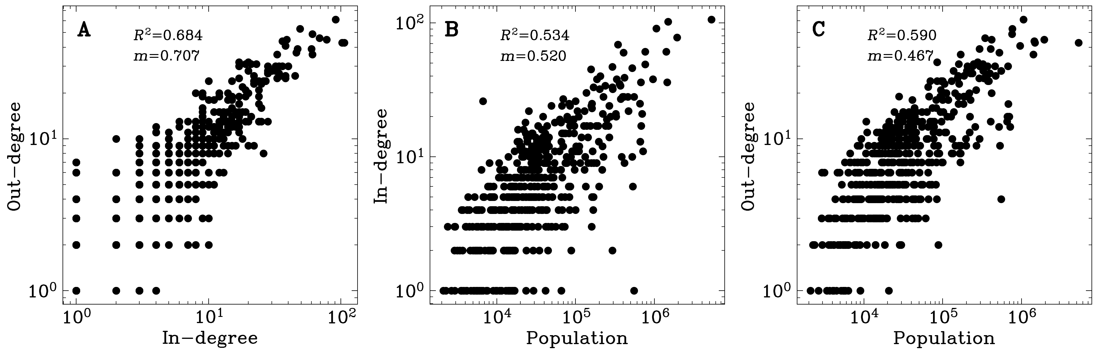
Figure A2: Relationships between the unweighted in-degree, unweighted out-degree, and population of the node. A) Relationships between the unweighted in-degree and the unweighted out-degree in the overdose journey network excluding self-loops. B) Relationship between the unweighted out-degree and the population. C) Relationships between the unweighted in-degree and the population. In-degree and out-degree values have been incremented by one to ensure visibility in log-transformed space. The $R^{2}$ values represent correlations between log-transformed values to limit distortion from outliers. The $m$ values represent the slopes of the linear regression in the log-transformed space.

We investigate relationships between the weighted in-degree, weighted out-degree, and the population. Because the network degrees and city populations often obey heavy-tailed distributions [39], we take the logarithm of these three quantities and show the scattergram and $R^{2}$ between each pair of the quantities in Figure 2. The figure indicates that these three quantities are strongly positively correlated with each other. We also observe slightly sub-linear relationships for the weighted degrees as a function of the population, which suggests a saturation effect of high-population counties as destinations and sources of overdose behavior (Figure 2B and C). These results are qualitatively the same for unweighted in- and out-degrees, although the correlation is weaker (see Figure A2).

We define outlier points as those whose absolute value of the residual obtained from the linear regression in the log-transformed space exceeds three standard deviations. We show the outlier points in red in Figure 2. Of particular interest is the one locale that is an outlier in both Figure 2B and C (indicated with a blue arrow), representing disproportionately low geographically discordant overdose activity. This locale is a particularly Hispanic and Latino medium metropolitan area that serves as a commuter county for three nearby large metropolitan areas.

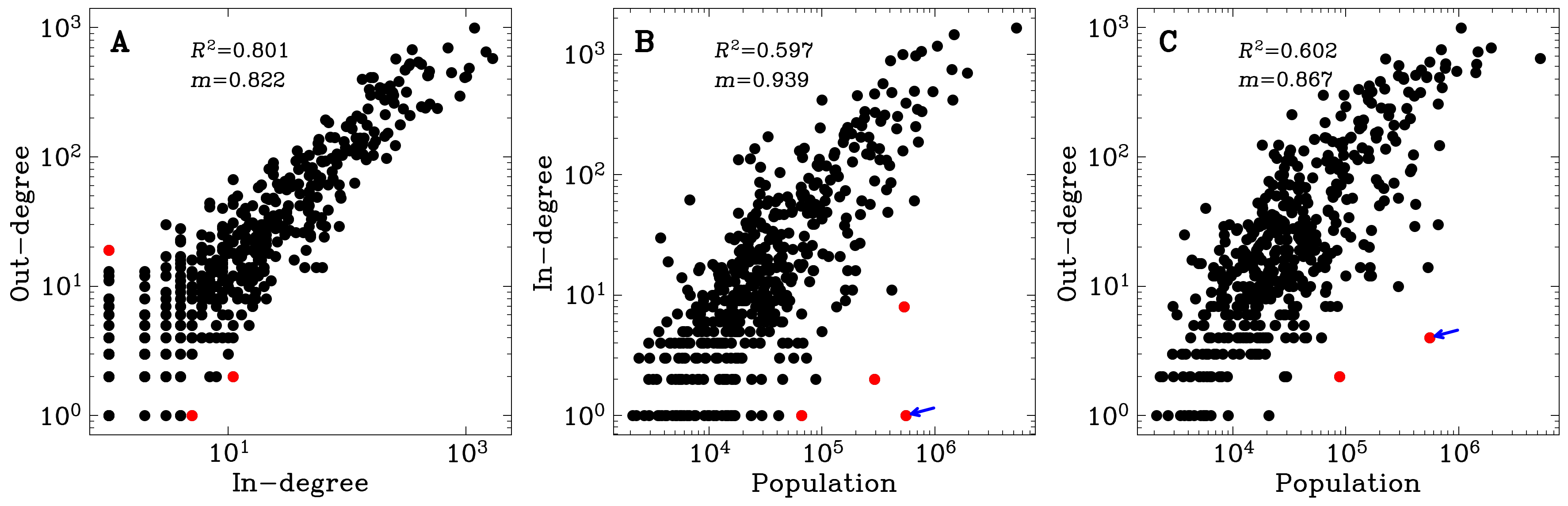
Figure 2: Relationships between the weighted in-degree, weighted out-degree, and population of the node. A) Relationships between the weighted in-degree and the weighted out-degree in the overdose journey network excluding self-loops. B) Relationship between the weighted out-degree and the population. C) Relationships between the weighted in-degree and the population. In-degree and out-degree values have been incremented by one to ensure visibility in log-transformed space. The $R^{2}$ values represent correlations between log-transformed values. The $m$ values represent the slopes of the linear regression in the log-transformed space. Outlier points, i.e., locales for which the magnitude of the residuals between observed values and those predicted by the linear regression exceed three standard deviations, are highlighted in red. The blue arrows indicate the locale that is an outlier in both panels B and C.

Table 2: Urbanization, demographic, and socioeconomic profiles of the top ten locales by in-degree per capita (top IPC) and out-degree per capita (top OPC), compared to the remaining locales. AI/AN stands for American Indian and Alaska Native; NHPI stands for Native Hawaiian and other Pacific Islander. Poverty refers to the fraction of the population living below poverty level. The urbanicity values are not population-weighted. Urbanization categories are collapsed into urban and rural per Section 2.2; the corresponding results for the uncollapsed urbanization categories are shown in Table A1.

	Category	Top IPC	Top OPC	Other
Population	Mean Population	1384559	1370947	67088
Urbanicity	Urban	100.0 %	100.0 %	40.58 %
	Rural	0.0 %	0.0 %	50.43 %
Race and	White Alone	53.88 %	55.66 %	72.44 %
Ethnicity	Black Alone	26.83 %	24.21 %	15.48 %
	AI/AN Alone	0.352 %	0.331%	1.019 %
	Asian Alone	5.365 %	5.579 %	2.341 %
	NHPI Alone	0.056 %	0.048 %	0.107 %
	Hispanic or Latino	21.72 %	23.09 %	11.85 %
Economic	Employed	52.84 %	52.68 %	47.95 %
	Poverty	12.90 %	12.30 %	12.85 %

To better understand focal points of geographically discordant overdose activity, we consider the top ten nodes by the weighted in-degree per capita (top IPC locales) and top ten nodes by the weighted out-degree per capita (top OPC locales), representing disproportionately high imports and exports of opioid overdoses when normalized by locale population. Even after adjusting for population size, these top nodes are exclusively urban locales (Table 2), but they do not simply reflect the largest cities; the top IPC locales are roughly equally represented across large central metro, large fringe metro, and medium metro areas, whereas the top OPC locales are concentrated in large central metro and large fringe metro areas (Table A1). Notably, the top IPC and top OPC locales have populations an order of magnitude larger and significantly higher employment rates than locales that are neither. This may be explained by differences in urbanicity alone: cities are larger and have more jobs than non-cities. The group difference between the top IPC locales and the others in terms of poverty rate is not statistically significant ($p=0.677$). All other group differences are significant ($p<0.05$); the test results are provided in Table A3.

3.3 HITS analysis

We similarly characterize in Table 3 the nodes with the highest authority and hub scores in comparison to all other locales. Hubs and authorities are over-represented in large fringe metro areas (Table A2). However, despite its name, a large fringe metro county in a large MSA may have a relatively small population because urban-rural classifications depend on MSA populations. In fact, on average, while the top authorities have approximately 17% larger populations than the top IPC and OPC locales, the top hubs have less than 50% of populations than the top authorities and less than 40% than the top IPC and OPC locales (see Table 3). This result is in stark contrast with the observation that the mean population is only approximately 1% different between the top IPC and the top OPC locales (Table 2). Additionally, hub nodes have a lower poverty rate than the top authorities or the other nodes. All reported group differences are significant with $p<0.001$; the test results are provided in Table A3.

Table 3: Urbanization, demographic, and socioeconomic profiles of the top ten and authorities and hubs, compared to the remaining locales. AI/AN stands for American Indian and Alaska Native; NHPI stands for Native Hawaiian and other Pacific Islander. Poverty refers to the fraction of the population living below poverty level. The urbanicity values are not population-weighted. Urbanization categories are collapsed into urban and rural per Section 2.2; the corresponding results for the uncollapsed urbanization categories are shown in Table A2.

	Category	Authority	Hub	Other
Population	Mean Population	1615255	783290	77239
Urbanicity	Urban	100.0 %	100.0 %	40.55 %
	Rural	0.0 %	0.0 %	59.46 %
Race and	White Alone	53.99 %	61.46 %	69.56 %
Ethnicity	Black Alone	23.73 %	18.09 %	18.03 %
	AI/AN Alone	0.445 %	0.380 %	0.876 %
	Asian Alone	6.262 %	4.842 %	2.597 %
	NHPI Alone	0.044 %	0.054 %	0.103 %
	Hispanic or Latino	23.86 %	26.97 %	12.49 %
Economic	Employed	52.84 %	53.62 %	48.59 %
	Poverty	12.57 %	9.780 %	13.02 %

3.4 Lengths of geographically discordant overdose journeys

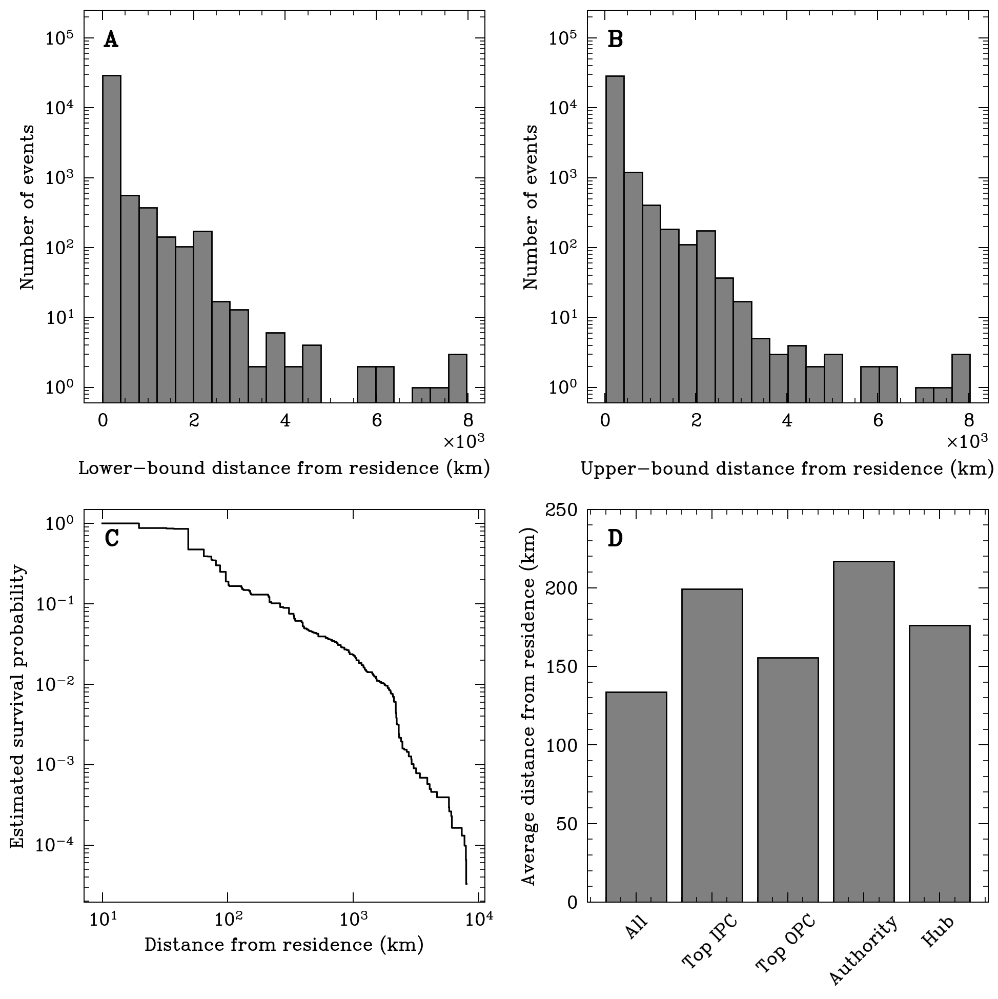
Figure 3: Distribution of distances of geographically discordant overdose journeys. A) Empirical distribution of lower-bound distances among the journeys. B) Empirical distribution of upper-bound distances. C) Estimated survival function of the journey distance. D) Average distance of geographically discordant overdose journeys. “All” refers to all journeys; “Top IPC” and “Authority” refer to journeys to the top IPC and authority nodes, respectively. “Top OPC” and “Hub” refer to journeys from the top OPC and hub nodes, respectively.

Figure 3 shows the distribution of journey-to-overdose lengths, denoted by $d$, among the geographically discordant overdose events. The histogram mass to the right of a particular lower-bound distance $d$ represents the number of events recorded at least $d$ (Figure 3A). Similarly, the histogram mass to the left of a particular upper-bound distance $d$ represents the number of events recorded at most $d$ (Figure 3B). From these lower-bound and upper-bound distances, we estimate the distribution of journey distances as described in Section 2.8. Figure 3C displays the resultant estimated complementary CDF (i.e., survival function) of $d$.

The median distance of geographically discordant overdose journeys is $49.42$ km, $10\%$ of the journeys exceed $262.1$ km, and $5\%$ exceed $407.4$ km. The average distance of these journeys is $133.8$ km (Figure 3D). Unsurprisingly, events are more common close to the home of a person who experienced an overdose, but we also find incidents over 8000 kilometers from the person who experienced an overdose’s residence. Figure 3C indicates a heavy-tailed nature of the distribution. Indeed, the coefficient of variation (CV) of $d$, i.e., the standard deviation of $d$ divided by the mean of $d$, is substantially larger than $1$ ($\text{CV}=2.299$), indicating that the distribution of $d$ has a heavier tail than the exponential distribution.

In Figure 3D, we interpret the journey-to-overdose distance as an import or export radius; in particular, we investigate the average journey-to-overdose distance to importers for the top IPC and authority nodes and from exporters for the top OPC and hub nodes. As reference, we also show the journey distance averaged over all the journeys (see the “All” bar in Figure 3D). The geographically discordant overdose journey from the residence to the top IPC nodes and from the top OPC nodes to their destinations are both longer, on average, than the mean journey. Furthermore, the journey distance for the top IPC nodes is larger than that for the top OPC nodes on average. As expected, the average journey distance to the top authority nodes and from the top hub nodes show qualitatively the same behavior as that to the top IPC nodes and that from the top OPC nodes, respectively. In other words, the average distance to the top authority nodes is larger than that from the top hub nodes, and the latter is larger than the average over all geographically discordant journeys. However, the effects of authorities and hubs are not a straightforward consequence of the general fact that authorities and hubs tend to be nodes with large in-degrees and large out-degrees, respectively. In fact, Figure 3D suggests that the average journey distance is larger for the top authority nodes than the top IPC nodes and larger for the top hub nodes than the top OPC nodes. See the “Monte Carlo U-Test” and “Z-Test” columns of Table A4 for statistical results.

3.5 Temporal aspects

We decompose the overdose journey network into a time series of overdose journey networks by constructing the network for each six-month time window. We show the time series of the share of the self-loops and the average journey distance in Figure 4A and B, respectively, in which each data point represents a six-month time window. The portion of the overdose events occurring in the person’s home locale increased modestly throughout 2018 to 2023 ($p<0.001$; Figure 4A). The average journey distance for geographically discordant overdose events did not systematically increase or decrease over the same five years, with the exception of a brief spike in the journey distance after the onset of the COVID-19 pandemic, which is shown by the dashed line (Figure 4B).

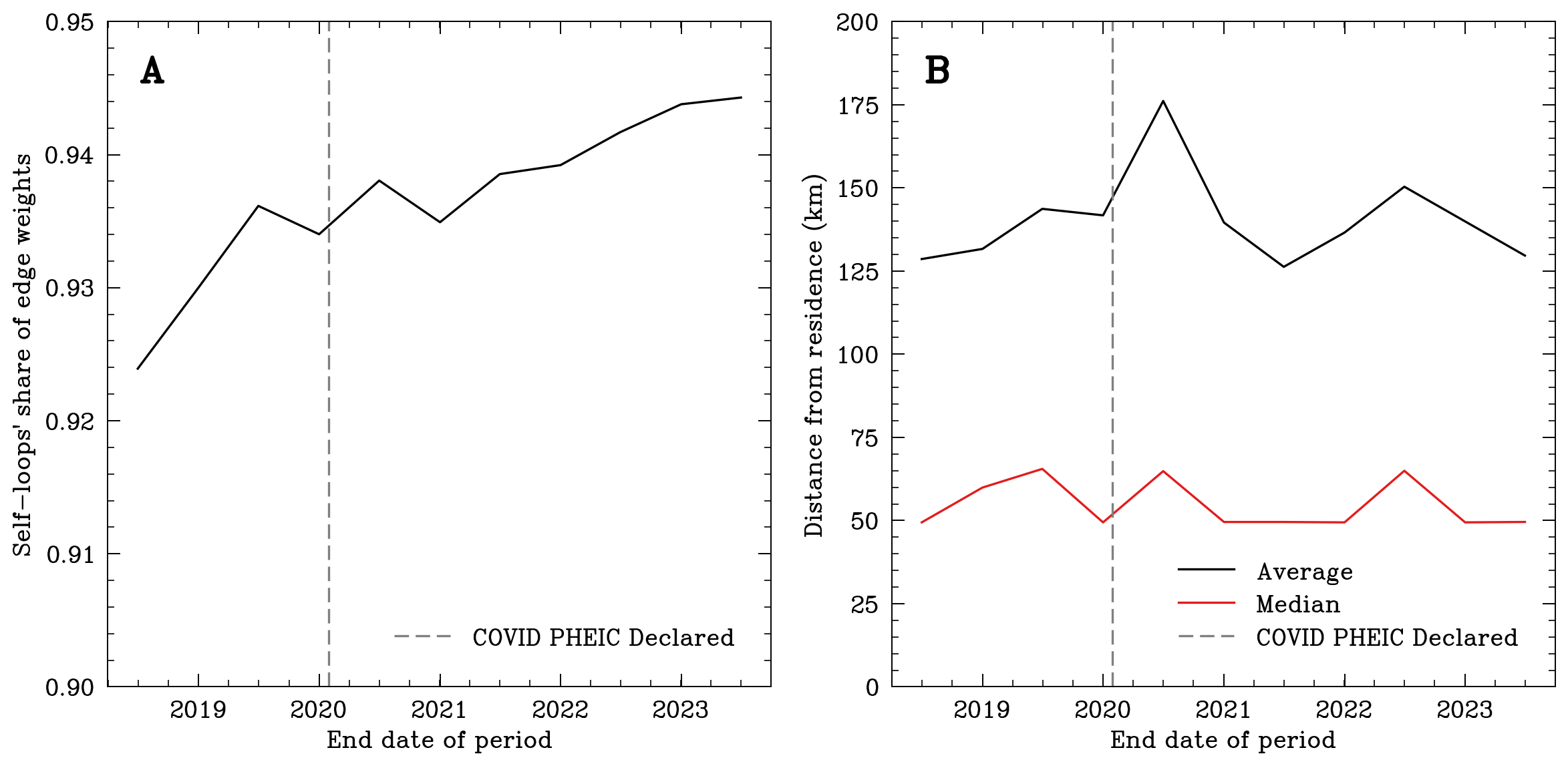
Figure 4: Time courses of the fraction of self-loops and the overdose journey distance. A) Fraction of edge weights owing to self-loops, indicating the portion of overdose events occurring in the home locale of the person who experienced an overdose. B) Average and median journey distance for geographically discordant events. The dashed lines indicate the date at which the World Health Organization declared the beginning of the COVID-19 Public Health Emergency of International Concern (PHEIC) [40].

Whether edges of the journey network are consistently present from one time period to another is relevant for public health applications; such persistence reflects enduring overdose-related transit patterns that may warrant policy intervention. To quantify the persistence of edges, we obtain the undirected temporal correlation coefficient $\gamma=0.304$. Further, focal importers and exporters (i.e., the top IPC, OPC, authority, and hub nodes) exhibit a significantly greater probability of (undirected) incident edge persistence than the average over all nodes ($p<0.05$), with $\gamma$ nearly double the network’s average (Figure 5A). Approximately the same results hold true in the directed setting, as well: focal importers and exporters also have significantly greater in- and out- temporal correlation coefficients than the network’s average ($p<0.05$, Figure 5B).

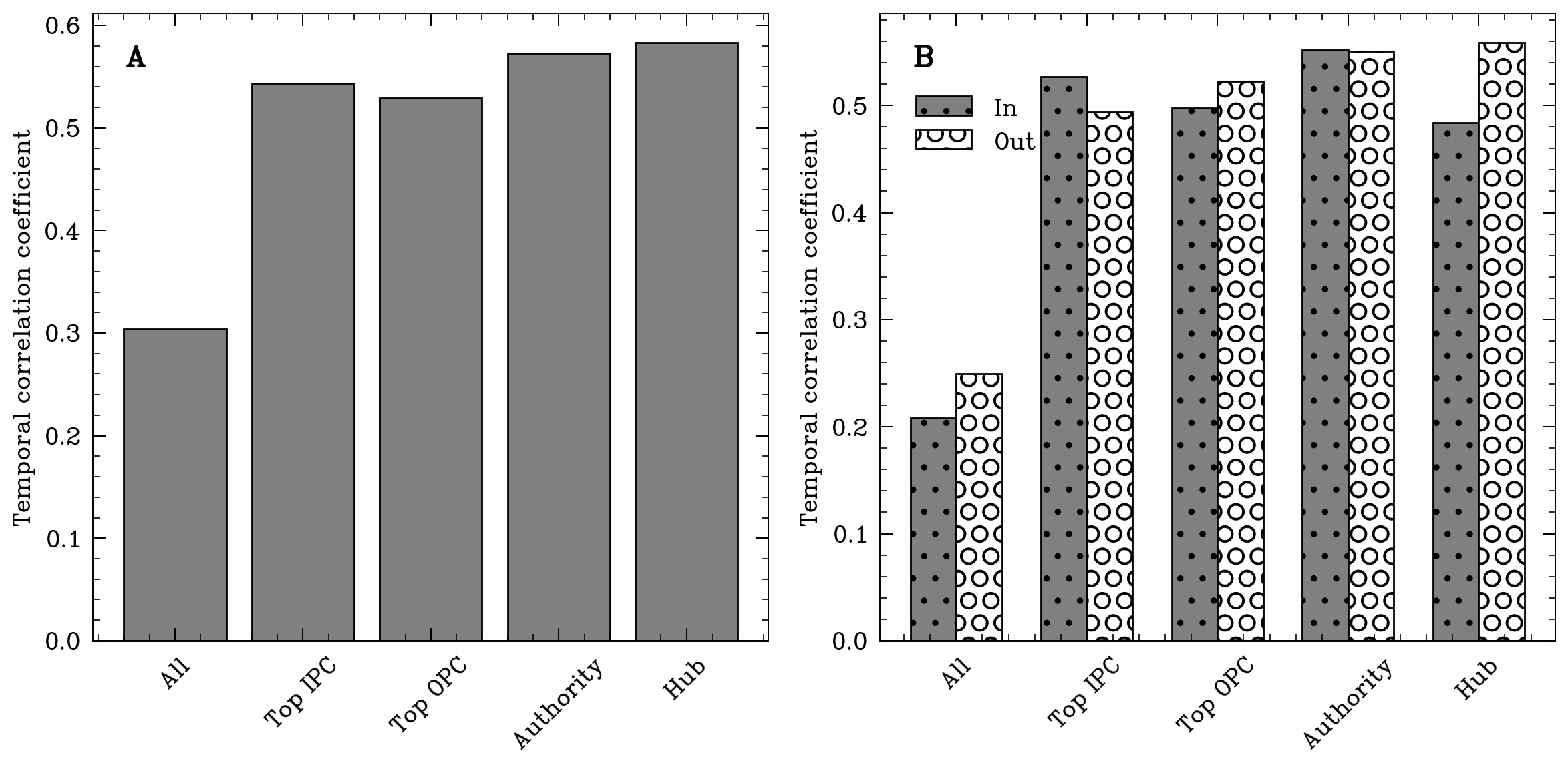
Figure 5: Persistence of edges in the temporal overdose journey network. A) Average undirected temporal correlation coefficients for all nodes, and the top IPC, OPC, authority, and hub nodes. B) Average directed (i.e., in- and out-) temporal correlation coefficients for all nodes, and the top IPC, OPC, authority, and hub nodes.

4 Discussion

We analyzed a spatial network of opioid-involved overdose journeys from $19$ states across the U.S. constructed from EMS records spanning 2018–2023. Our work underscores that the opioid overdose epidemic does not only exist where overdoses occur. Patterns of import and export of overdose behavior across county borders emerge, as $6.2\%$ of opioid-involved overdose events occurred outside the residential FIPS code of the person who experienced an overdose. We focused on these geographically discordant events, of which roughly $10\%$ occurred over 262 km from the home of the person who experienced an overdose.

Public health authorities may wish to identify and intervene at focal points of import/export behavior, but it is not necessarily clear how to define them. In this work, we considered two such approaches: measures calculable from normalized travel counts involving the county alone (i.e., IPC and OPC) and network-based measures (i.e., authorities and hubs). Focal locales according to these measures tended to be urban, were higher in Asian and Hispanic or Latino populations, were lower in white, American Indian and Alaska Native, and Native Hawaiian and other Pacific Islander populations, and had a larger employment rate, population, journey distance, and edge persistence than the average over all the edges in the network.

We found that some aspects of overdose journeys differed between the types of focal points. For instance, the top IPC, OPC, and authority locales have population sizes of the same order of magnitude on average, but the top hubs are much smaller in population, although they are much larger than the average over all locales. Additionally, the overdose journeys to the top IPC and authority nodes were longer than those from the top OPC and hub nodes on average. This result may be partly explained by size and resource advantage: the average population of authorities is more than twice that of hubs, and larger locales may provide more resources for opioid users [41].

We contend that indirect paths in the overdose journey network do not have functional meanings for the following reason: If there is an indirect path from the $i$th to the $\ell$th nodes, then $A_{ij}=1$ and $A_{j\ell}=1$, which implies that there is an overdose journey from the $i$th to the $j$th nodes, made by individual $u_{1}$, and another journey from the $j$th to the $\ell$th nodes, made by individual $u_{2}$. In this situation, it is unlikely that $u_{1}$ influences $u_{2}$ to trigger $u_{2}$’s overdose behavior outside $u_{2}$’s residence. The same reasoning holds true even if edges are weighted or we consider the effects of mass media or social media. The difficulty of interpretation of indirect paths may limit the utility of network analysis as an approach, rendering only the direct path effects such as the in- and out-degrees relevant to overdose behavior. However, we found that the HITS algorithm, which exploits effects of the indirect paths (e.g., hub scores of nodes are large when they send edges to authorities, which are nodes that tend to receive edges from hubs), reveals features of overdose journeys that were beyond the prediction by the top IPC or OPC nodes. Specifically, the top authority and hub nodes had larger journey distances than the top IPC and OPC nodes, respectively. In addition, the top authorities and hubs tend to be concentrated in large fringe metropolitan areas, whereas top IPC and OPC locales are more dispersed across large central metropolitan, large fringe metropolitan, and medium metropolitan areas. These results suggest that the authorities and hubs, which tend to be interconnected with each other, may form a scaffold of the overdose journey network and have particular properties compared to top IPC and OPC nodes. Further investigating this issue in combination with other data sources, demographic information, and geographic information, with potentially improved coverage and accuracy of the EMS records, warrants future work.

We showed in Section 3.5 that the share of geographically discordant events decreased between 2018 and 2023. This result suggests that typical overdose events may be occurring closer to the home of the person who experienced an overdose in 2023 compared to in 2018. Monitoring the same data for some more years is expected to reveal whether this effect is triggered by the COVID-19 pandemic starting in year 2020. Such a finding would be consistent with recent evidence from Rhode Island suggesting that drug overdose deaths occurring in residences of the people who experienced overdoses increased disproportionately from $2019$ to $2020$, compared to those occurring in any location [42].

Our estimate of the fraction of geographically discordant overdose events is much lower than the 25% reported in a recent study [14]. This difference may be caused by the differently sized geographic units: counties in the present study versus census tracts in their study. Our larger scale of analysis enabled us to identify inter-county overdose journeys and analyze the distribution of overdose journey distances. Another advancement of the present study relative to theirs is that we compared between authority nodes and top IPC nodes and between hub nodes and top OPC nodes. With the latter analysis, we provided evidence supporting that the HITS algorithm provides unique information about overdose journeys that simpler pairwise analysis does not.

Our work has at least three potential limitations. First, we restricted our analysis to the counties with at least 75% UEC for the entire five-year period. Doing so is standard for the present data set [3] but excludes many locales (Section 2.1). Future data collection efforts may mitigate this limitation, as the number of reporting locales increases. Second, we focused on non-fatal opioid-involved overdose events, which may mean our characterizations of journey lengths is not fully representative of high-mortality locales. Third, we geographically censored the EMS event records at the county-equivalent level. Therefore, we make no claims about spatial dynamics for within-county overdose journeys. Future work may aim to narrow these data gaps to draw more granular insights regarding the national character of overdose journeys. Future work can also focus on different types of drugs, such as stimulants, to compare the spatial dynamics of different non-fatal overdoses across the country.

We highlight the value of leveraging large-scale EMS data for understanding the spatial dynamics of the opioid crisis. One potential avenue for future research is to leverage agent-based simulations to better understand the efficacy of targeting authorities and hubs for public health interventions. A second future research thrust is to better understand the especially long overdose journeys highlighted in this study. In Section 3.4, we discuss the surprising number of incidents occurring at least $8000$ km from the home of the person who experienced an overdose. We emphasize, however, that people who experienced overdoses did not necessarily travel such distances on the days of their incidents. For instance, not all individuals (e.g., those experiencing homelessness) functionally reside in their official residence of record for the entire year. Additionally, EMS place-of-residence information is sometimes collected from historical patient records, which may be out-of-date or inaccurate due to clerical errors. Further research is required to better understand the etiology of these particularly long overdose journeys.

Declarations

Availability of data and materials

Data were provided by biospatial through an existing data use agreement with the Centers for Disease Control and Prevention, National Center for Injury Prevention and Control. Due to the existing clauses of the data use agreement, we do not make the data available for public release. The list of hub and authority locales, however, is accessible at reasonable request of the authors.

Acknowledgements

We are grateful for the contributors who developed the open-source software used in this work, including Cartopy [43], lifelines [44], NetworkX [45], NumPy [46], pyMannKendall [47], SciPy [48], smplotlib [49], and statsmodels [50]. Additionally, we are appreciative of municipalities sharing data with biospatial, Inc.; Freelancer Technology Pty Limited for programmatic support; and Josh Walters for assistance involving the biospatial platform.

Authors’ contributions

LHM, NM, ND, and RL, conceptualized the study. LHM, NM, and SC provided the methods. LHM implemented the methods, analyzed the data, and generated the visualizations. LHM and NM mainly wrote the manuscript, with contributions from SC, ND, and RL. All authors discussed the methods and results and reviewed the manuscript.

Funding

This material is based upon work supported by the Centers for Disease Control and Prevention under Contract No. NOIS2-096. SC, AA, and RL are employed by the Centers for Disease Control and Prevention, National Center for Injury Prevention and Control, which also funded this work.

Competing interests

The authors declare that they have no competing interests.

Appendix A Supplementary materials

A.1 Top k selection

Throughout this work, we consider top $k$ locales across four metrics. To set the $k$ value, we first sort the weighted in-degree per capita, weighted out-degree per capita, hub score, and authority score, of all the locales. Then, for each of these metrics, we calculate the elbow point (i.e., the metric value yielding the maximum curvature) using the offline Kneedle algorithm. We set the algorithm’s sensitivity parameter $S$ to $0$, which is recommended in perfect information settings [51].

This process reveals elbow values of $11$, $10$, $4$, and $4$ for weighted in-degree per capita, weighted out-degree per capita, authority scores, and hub scores, respectively (Figure A1). In the interest of readability, interpretability, and consistency, we use $k=10$ for all the four metrics. This $k$ value is round numbers close to or equal to the elbow values for the IPC and OPC, respectively. It is important to use the same $k$ value across the four measures because we compare observations from the top $k$ nodes (e.g., average distance of geographically discordant overdose journey over the top $k$ nodes) across the four measures.

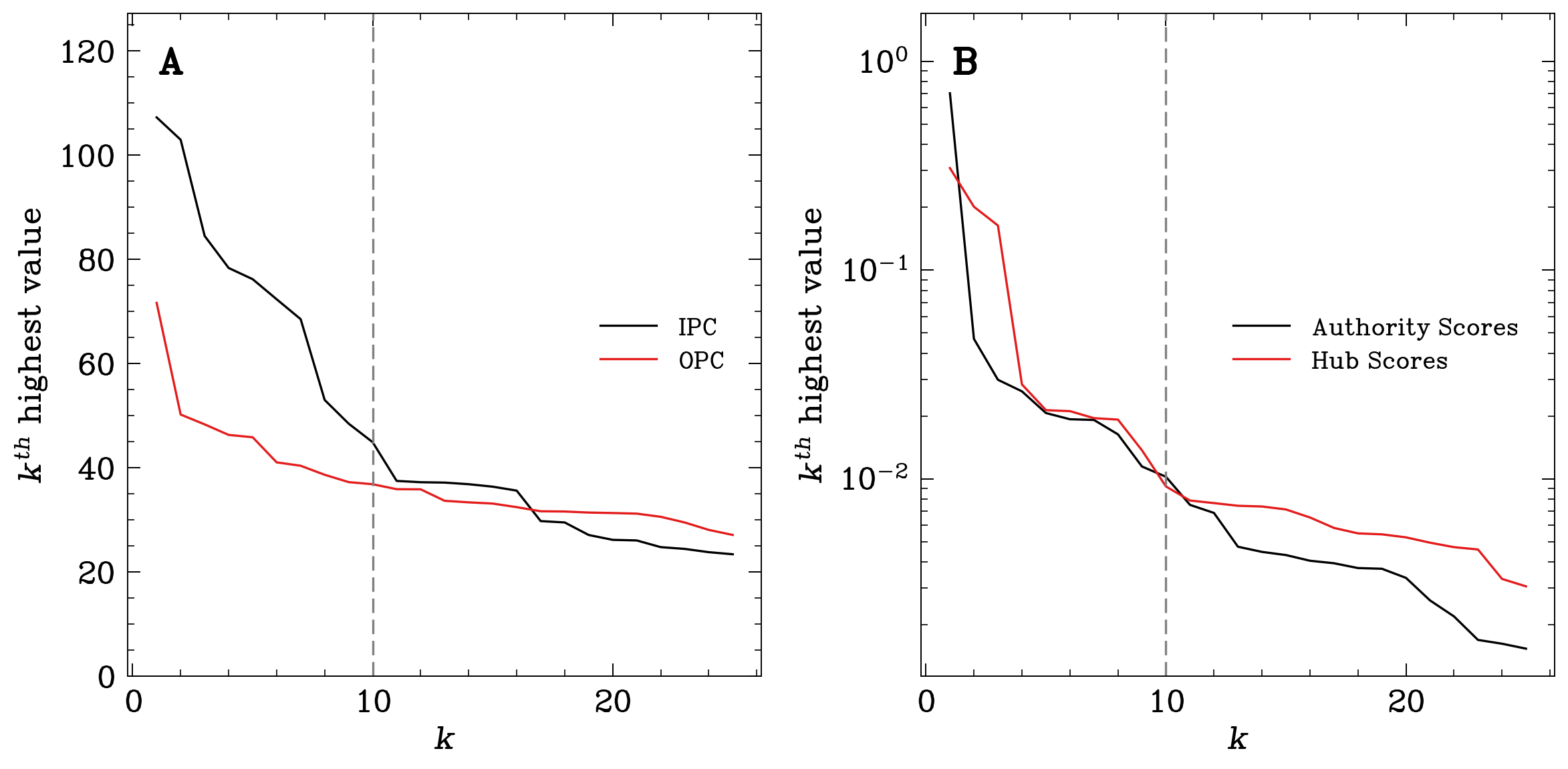
Figure A1: Sorted IPC, OPC, authority, and hub values. A) Sorted IPC and OPC values. B) Sorted authority and hub scores. The dashed lines represent $k=10$.

A.2 Unweighted degree analysis

A.3 Locale profiles with uncollapsed urbanization categories

Table A1: Urbanization profiles of the top ten locales by in-degree per capita (top IPCs) and out-degree per capita (top OPCs), compared to the remaining locales. Values are not population-weighted.

	Category	Top IPC	Top OPC	Other
Urbanicity	Large central metro	40.0 %	30.0 %	1.109 %
	Large fringe metro	30.0 %	60.0 %	13.75 %
	Medium metro	30.0 %	10.0 %	13.30 %
	Small metro	0.0 %	0.0 %	12.42 %
	Micropolitan	0.0 %	0.0 %	17.52 %
	Noncore	0.0 %	0.0 %	41.91 %

Table A2: Urbanization profiles of the top ten authorities and hubs, compared to the remaining locales. Values are not population-weighted.

	Category	Authority	Hub	Other
Urbanicity	Large central metro	20.0 %	0.0 %	1.891 %
	Large fringe metro	80.0 %	100.0 %	13.24 %
	Medium metro	0.0 %	0.0 %	13.45 %
	Small metro	0.0 %	0.0 %	11.97 %
	Micropolitan	0.0 %	0.0 %	16.81 %
	Noncore	0.0 %	0.0 %	42.65 %

A.4 Statistical results

	Population	Race & Ethnicity	Employed	Poverty
Top IPC vs. Top OPC	***	***	*	***
Top IPC vs. Other	***	***	***
Top OPC vs. Other	***	***	***	***
Authority vs.  Hub	***	***	***	***
Authority vs. Other	***	***	***	***
Hub vs. Other	***	***	***	***

Table A3: Statistical results for pairwise comparison between any two of the top IPC, top OPC, and the other nodes and between any two of the top authority, top hub, and the other nodes. We ran the Tukey’s HSD test, which corrects for multiple comparisons [34], for “Population,” which refers to the total population size. We used the contingency table-based G-test of independence [32] for “Race & Ethnicity,”, “Employed,” and “Poverty.” *: $p=0.05$, **: $p=0.01$, and ***: $p=0.001$. All the results obtained with the G-test are Holm-Bonferroni-corrected for $\binom{3}{2}=3$ comparisons [37].

	Journey Distance		Temporal Correlation
	Monte Carlo U-Test	Z-Test	HSD Test (Undirected)	HSD Test (In)	HSD Test (Out)
All vs. Top IPC	***	***	*	***	*
All vs. Top OPC	***	***	*	**	**
All vs. Authority	***	***	**	***	***
All vs. Hub	***	***	**	**	***
Top IPC vs. Top OPC	***	***
Top IPC vs. Authority		**
Top IPC vs. Hub
Top OPC vs. Authority	***	***
Top OPC vs. Hub	***	**
Authority vs. Hub		***

Table A4: Statistical results for pairwise comparisons of the journey distances and average temporal correlation coefficients. The “Monte Carlo U-Test” and “Z-Test” columns reflect the results for journey distances, for which we ran the Monte Carlo U-test and Z-test described in Section 2.8. The “HSD Test (Undirected),” “HSD Test (In),” and “HSD Test (Out)” columns reflect results for undirected temporal correlation coefficients, in- temporal correlation coefficients, and out- temporal correlation coefficients, respectively, for which we ran Tukey’s HSD test [34]. *: $p=0.05$, **: $p=0.01$, and ***: $p=0.001$. All the results are Holm-Bonferroni-corrected for $\binom{5}{2}=10$ comparisons [37], with the exception of HSD tests, which already correct for multiple comparisons.

References

- [1] Merianne Rose Spencer, Arialdi M Miniño and Margaret Warner “Drug Overdose Deaths in the United States, 2001–2021”, 2022, pp. 1–8
- [2] Hawre Jalal et al. “Changing dynamics of the drug overdose epidemic in the United States from 1979 through 2016” In Science 361.6408 American Association for the Advancement of Science, 2018, pp. eaau1184
- [3] Shannon M Casillas et al. “Patient-Level and County-Level Trends in Nonfatal Opioid-Involved Overdose Emergency Medical Services Encounters—491 Counties, United States, January 2018–March 2022” In Morbidity and Mortality Weekly Report 71.34 Centers for Disease ControlPrevention, 2022, pp. 1073
- [4] Richard C Dart et al. “Trends in Opioid Analgesic Abuse and Mortality in the United States” In New England Journal of Medicine 372.3 Mass Medical Soc, 2015, pp. 241–248
- [5] Byungkyu Lee et al. “Systematic Evaluation of State Policy Interventions Targeting the US Opioid Epidemic, 2007-2018” In JAMA Network Open 4.2 American Medical Association, 2021, pp. e2036687–e2036687
- [6] Douglas A Luke and Jenine K Harris “Network Analysis in Public Health: History, Methods, and Applications” In Annual Review of Public Health 28 Annual Reviews, 2007, pp. 69–93
- [7] Douglas A Luke and Katherine A Stamatakis “Systems Science Methods in Public Health: Dynamics, Networks, and Agents” In Annual Review of Public Health 33, 2012, pp. 357–376
- [8] T W Valente and S R Pitts “An Appraisal of Social Network Theory and Analysis as Applied to Public Health: Challenges and Opportunities” In Annual Review of Public Health 38, 2017, pp. 103–118
- [9] Abby E Rudolph, April M Young and Jennifer R Havens “Using Network and Spatial Data to Better Target Overdose Prevention Strategies in Rural Appalachia” In Journal of Urban Health 96.1 Springer, 2019, pp. 27–37
- [10] Brea L Perry et al. “Co-prescription network reveals social dynamics of opioid doctor shopping” In PLoS ONE 14.10 Public Library of Science San Francisco, CA USA, 2019, pp. e0223849
- [11] Kai-Cheng Yang et al. “Comparing measures of centrality in bipartite patient-prescriber networks: A study of drug seeking for opioid analgesics” In PLoS ONE 17.8 Public Library of Science San Francisco, CA USA, 2022, pp. e0273569
- [12] Carrie B Oser and Kathi L H Harp “Treatment Outcomes for Prescription Drug Misusers: The Negative Effect of Geographic Discordance” In Journal of Substance Abuse Treatment 48.1 Elsevier, 2015, pp. 77–84
- [13] Lallen T Johnson, Ralph B Taylor and Jerry H Ratcliffe “Need Drugs, Will Travel?: The Distances to Crime of Illegal Drug Buyers” In Journal of Criminal Justice 41.3 Elsevier, 2013, pp. 178–187
- [14] Amir Forati, Rina Ghose, Fahimeh Mohebbi and John R Mantsch “The journey to overdose: Using spatial social network analysis as a novel framework to study geographic discordance in overdose deaths” In Drug and Alcohol Dependence 245 Elsevier, 2023, pp. 109827
- [15] “biospatial.io”, https://www.biospatial.io/, 2023
- [16] Council State and Territorial Epidemiologists “Emergency Medical Services Nonfatal Opioid Overdose Standard Guidance” Accessed: September 24, 2023, 2022
- [17] U.S. Bureau “American Community Survey 2017-2021 5-Year Data Release”, American Community Survey 5-year estimates, 2021 URL: https://www.census.gov/newsroom/press-kits/2022/acs-5-year.html
- [18] Deborah D Ingram and Sheila J Franco “2013 NCHS Urban-Rural Classification Scheme for Counties” In Vital and Health Statistics US Department of HealthHuman Services, Centers for Disease ControlPrevention, National Center for Health Statistics, 2014, pp. 1–73
- [19] National Weather Service “U.S. Counties” Shape files derived from TIGER 2000. Date uploaded: 2023-06-30, 2023 URL: https://www.weather.gov/gis/Counties
- [20] Mark E J Newman, Stephanie Forrest and Justin Balthrop “Email networks and the spread of computer viruses” In Physical Review E 66.3 APS, 2002, pp. 035101
- [21] Diego Garlaschelli and Maria I Loffredo “Patterns of Link Reciprocity in Directed Networks” In Physical Review Letters 93.26 APS, 2004, pp. 268701
- [22] Mark E J Newman “Networks” Oxford, UK: Oxford University Press, 2018
- [23] Jon M Kleinberg “Authoritative sources in a hyperlinked environment” In Journal of the ACM 46.5 ACM New York, NY, USA, 1999, pp. 604–632
- [24] Aaron Clauset and Nathan Eagle “Persistence and periodicity in a dynamic proximity network” In Proceedings of the DIMACS Workshop on Computational Methods for Dynamic Interaction Networks, 2007
- [25] John Tang et al. “Small-world behavior in time-varying graphs” In Physical Review E 81.5 APS, 2010, pp. 055101
- [26] Vincenzo Nicosia et al. “Graph Metrics for Temporal Networks” In Temporal Networks Berlin, DE: Springer, 2013, pp. 15–40
- [27] N. Masuda and R. Lambiotte “A Guide to Temporal Networks” Singapore: World Scientific, 2020
- [28] Kathrin Büttner, Jennifer Salau and Joachim Krieter “Temporal correlation coefficient for directed networks” In SpringerPlus 5.1 Springer, 2016, pp. 1–17
- [29] Lucas H McCabe “Nonparametric Estimation and Comparison of Distance Distributions from Censored Data” In arXiv preprint arXiv:2311.02658, 2023
- [30] Edward L Kaplan and Paul Meier “Nonparametric Estimation from Incomplete Observations” In Journal of the American Statistical Association 53.282 Taylor & Francis, 1958, pp. 457–481
- [31] Bruce W Turnbull “The Empirical Distribution Function with Arbitrarily Grouped, Censored and Truncated Data” In Journal of the Royal Statistical Society: Series B (Methodological) 38.3 Wiley Online Library, 1976, pp. 290–295
- [32] John H McDonald “G–test of goodness-of-fit” In Handbook of Biological Statistics Baltimore, MD: Sparky House Publishing, 2014, pp. 53–58
- [33] Robert R Sokal and F James Rohlf “Introduction to Biostatistics” San Francisco, CA: Dover, 1987
- [34] Hervé Abdi and Lynne J Williams “Tukey’s Honestly Significant Difference (HSD) Test” In Encyclopedia of Research Design 3.1 Sage Thousand Oaks, CA, 2010, pp. 1–5
- [35] Khaled H Hamed and A Ramachandra Rao “A modified Mann-Kendall trend test for autocorrelated data” In Journal of Hydrology 204.1-4 Elsevier, 1998, pp. 182–196
- [36] Maurice G Kendall “Rank Correlation Methods” London, UK: Charles Griffin, 1975
- [37] Sture Holm “A Simple Sequentially Rejective Multiple Test Procedure” In Scandinavian Journal of Statistics 6.2 JSTOR, 1979, pp. 65–70
- [38] Hervé Abdi “Holm’s Sequential Bonferroni Procedure” In Encyclopedia of Research Design 1.8 Thousand Oaks, California, 2010, pp. 1–8
- [39] Aaron Clauset, Cosma Rohilla Shalizi and Mark E J Newman “Power-Law Distributions in Empirical Data” In SIAM Review 51.4 SIAM, 2009, pp. 661–703
- [40] Leila Fadel and Nurith Aizenman “WHO Says COVID-19 Is No Longer a Global Health Emergency”, https://www.npr.org/2023/05/05/1174275727/who-says-covid-19-is-no-longer-a-global-health-emergency, 2023
- [41] Avik Chatterjee et al. “Broadening access to naloxone: Community predictors of standing order naloxone distribution in Massachusetts” In Drug and Alcohol Dependence 230 Elsevier, 2022, pp. 109190
- [42] Alexandria Macmadu et al. “Comparison of Characteristics of Deaths from Drug Overdose Before vs During the COVID-19 Pandemic in Rhode Island” In JAMA Network Open 4.9 American Medical Association, 2021, pp. e2125538–e2125538
- [43] Phil Elson et al. “SciTools/cartopy: v0.22.0” Zenodo, 2023
- [44] Cameron Davidson-Pilon “lifelines: survival analysis in Python” In Journal of Open Source Software 4.40 The Open Journal, 2019, pp. 1317
- [45] Aric Hagberg, Pieter Swart and Daniel Schult “Exploring network structure, dynamics, and function using NetworkX”, 2008
- [46] Charles R Harris et al. “Array programming with NumPy” In Nature 585.7825 Nature Publishing Group UK London, 2020, pp. 357–362
- [47] Md Hussain and Ishtiak Mahmud “pyMannKendall: a python package for non parametric Mann Kendall family of trend tests” In Journal of Open Source Software 4.39 The Open Journal, 2019, pp. 1–3
- [48] Pauli Virtanen et al. “SciPy 1.0: Fundamental Algorithms for Scientific Computing in Python” In Nature Methods 17.3 Nature Publishing Group, 2020, pp. 261–272
- [49] Jiaxuan Li “AstroJacobLi/smplotlib: v0.0.9” Zenodo, 2023
- [50] Skipper Seabold and Josef Perktold “Statsmodels: Econometric and Statistical Modeling with Python” In 9th Python in Science Conference, 2010
- [51] Ville Satopaa, Jeannie Albrecht, David Irwin and Barath Raghavan “Finding a ”Kneedle” in a Haystack: Detecting Knee Points in System Behavior” In 31st International Conference on Distributed Computing Systems Workshop, 2011, pp. 166–171 IEEE