Estimation of the lifetime distribution from fluctuations in Bellman-Harris processes

Abstract.

The growth of a population is often modeled as branching process where each individual at the end of its life is replaced by a certain number of offspring. An example of these branching models is the Bellman-Harris process, where the lifetime of individuals is assumed to be independent and identically distributed. Here, we are interested in the estimation of the parameters of the Bellman-Harris model, motivated by the estimation of cell division time. Lifetimes are distributed according a Gamma distribution and we follow a population that starts from a small number of individuals by performing time-resolved measurements of the population size. The exponential growth of the population size at the beginning offers an easy estimation of the mean of the lifetime. Going farther and describing lifetime variability is a challenging task however, due to the complexity of the fluctuations of non-Markovian branching processes. Using fine and recent results on these fluctuations [21], we describe two time-asymptotic regimes and explain how to estimate the parameters. Then, we both consider simulations and biological data to validate and discuss our method. The results described here provide a method to determine single-cell parameters from time-resolved measurements of populations without the need to track each individual or to know the details of the initial condition.

Keywords: Bellman-Harris process, asymptotic fluctuations, estimation, inverse problem, cell division

1. Introduction

Branching processes are widely used for modeling populations where individuals may reproduce or die, and evolve independently. The simplest Markovian branching process is the Galton-Watson process. In continuous time, each individual lives during an exponential time and is then replaced by a random number of offspring. This model and its extensions have been used and applied in population dynamics and evolution [17, 19, 23, 26], epidemiology [8, 12], queuing systems like polling [29], nuclear physics [15] etc. The exponential distribution of lifetimes corresponds to a memory less property and absence of aging of individuals.

For many models and issues in life sciences, such a distribution is not relevant and does not fit with data and observations. For instance, the time for cell division rather looks like an unimodal distribution, more or less concentrated around its mean, see e.g. [11, 27, 28] and references therein. The variability of lifespan can be attributed to different sources. Various models have been considered to describe it, including a trait driving the division (the time from birth, the size, the increment of size from birth) or taking into account environmental variability, or individual variability, see e.g.  [10, 14, 28]. Similarly, in epidemiology, the time of infection for an individual is not considered exponentially distributed [25]; rather, it is more accurately described by an unimodal time with a varying transmission rate. Another limitation of exponential law is that the value of the mean characterizes the full distribution and thus forces the variance of the distribution and the pattern of the variability.

Diverse extensions of the Galton-Watson process in continuous time enable to go beyond the exponential lifetimes and consider an age structure. In the Bellman-Harris process, the individuals live during independent random times that follow a common but general distribution. We are interested in inferring this distribution. In biology or ecology or epidemiology, many data (experimental data or observations in wild life) consist of measuring the total population size along time, with no access to the values of the lifespan between two counts. However, up to our knowledge, the estimation of the parameters of the lifetime distribution from such population-level monitoring has not attracted a lot of attention so far.

Our work aims at proposing efficient method for estimation of the parameters of the distribution of lifetimes from such data set. Going from the population sizes along a given time sequence to the growth rate of the population is direct by looking at the line observed from data plotted at the log scale. But going farther and obtaining the variance and more generally the quantification of variability of the lifespan of individuals is much more delicate in the non-exponential case. This is due to several reasons we are explaining in this work. Roughly for now, fluctuations of the population size around its predicted value can have different and subtle behaviors depending on the time distribution and the time of observations.

Our motivation for this work and our first application is the estimation of the time for cell division using microfluidics experiments. Indeed, single cell approaches have emerged as an important new way to address biological questions, with many formats to produce data that show heterogeneity of biological processes [30]. We are particularly interested in experiments based on anchored droplets, where the contents of each microfluidic drop can be followed in time [1]. These experiments allow to obtain many parallel realizations of the growth of cell population starting from a small number of cells [10]. We want to exploit such data to infer the variability of cell division time, using Bellman-Harris processes as a simple statistical framework to model individual variability without heredity, or with negligible heredity.

We choose here to focus on inference of the two parameters of Gamma lifetime distribution, with binary division. Indeed, Gamma distribution provides a convenient unimodal two parameters family which allows to cover realistic lifetime distribution. It is also a rare case among non-exponential laws which yields some explicit and useful computations. As we will see, fluctuations have a complex behavior, which is a general phenomenon for branching processes. It can be fully described here, thanks in particular to recent results on fluctuations of Crump-Mode-Jagers processes [21]. This result can be seen as a starting point for more complex explorations to link the fluctuations at the level of population to the individual variability. In particular, in Section 6.3, we deal with extension of the results to more general lifetimes and non-binary reproduction events.

Let us be more explicit now on the setting and the results. We consider two positive real numbers $k\geq 1,\theta>0$. The process starts from one single individual and each individual lives, independently, during a random time distributed as a Gamma distribution $\Gamma(k,\theta)$. The density $g_{k,\theta}$ of this law, denoted $g$ for short, is defined on $\mathbb{R}_{+}$ by

$$g_{k,\theta}(t)=g(t)=\frac{t^{k-1}e^{-\frac{t}{\theta}}}{\Gamma(k)\theta^{k}},$$

where $\Gamma(x)=\int_{0}^{\infty}s^{x-1}e^{-s}ds$ is the Gamma function. We denote by $(N_{t})_{t\geq 0}$ the number of individuals at time $t$ and the observed quantity is the number of individuals $(N_{t_{i}})_{i=1...n}$ for a given sequence of times $(t_{i})_{i=1...n}$. Our objective is to determine the two unknown values $k,\theta$ as precisely as possible. It is equivalent to determine the mean $\mu$ and variance $\sigma^{2}$ of the lifetime. For a $\Gamma(k,\theta)$ law, they are explicitly given by

$$\mu=k\theta,\qquad\sigma^{2}=k\theta^{2}.$$

Equivalently, we choose to infer the pair $(\mu,\sigma/\mu)=(k\theta,1/\sqrt{k})$ gathering the mean and coefficient of variation. Classically, in such setting, a first information comes from the observed Malthusian growth. Indeed, for Bellman-Harris processes under some general conditions [20, Theorem $17.1$ and $21.1$],

(1) $$\mathbb{E}(N_{t})\underset{t\rightarrow\infty}{\sim}n_{1}e^{\alpha t},\qquad N_{t}\underset{t\rightarrow\infty}{\sim}\mathbb{E}(N_{t})W\underset{t\rightarrow\infty}{\sim}n_{1}e^{\alpha t}W\,\text{ a.s.},$$

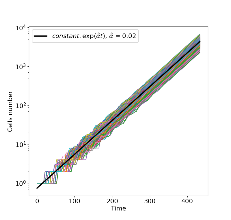
where $n_{1},\alpha>0$ and $W$ is a non-negative finite random variable. Besides, for $\Gamma(k,\theta)$ lifetime, $\alpha$ is explicitly known in function of $k,\theta$. Plotting the number of individuals observed at the log scale provides then the following first estimation

$$\frac{\log(N_{t})}{t}\underset{t\rightarrow\infty}{\longrightarrow}\alpha=\frac{1}{\theta}\left(2^{\frac{1}{k}}-1\right)\qquad\text{a.s.}.$$

With real data of biological growth, a “nice” line may indeed be observed during some suitable time window, namely after the biological lag phase and before the cell number approaches the carrying capacity of the droplet [10]. As such, this time window must avoid the early times for which the biological processes are not yet stationary. It also stops at large times when the independence and branching property fails due to competition.

The challenge is then to extract additional pertinent information from the data and to capture the two parameters $(k,\theta)$. We assume that we have many observations of the process, i.e. many realizations of the Bellman-Harris process and the values of the population size at different times. One may thus consider variance [27] of the number of individuals. For Gamma distribution,

(2) $$\lim_{t\rightarrow\infty}\frac{\text{Var}(N_{t})}{\mathbb{E}[N_{t}]^{2}}=q(\sigma/\mu),$$

where the function $q$ is explicit. This gives a theoretical way to conclude for estimation, and we refer to Section 6.2 for details.

However, various limitations exist for such an approach in practical applications. In particular, the microfluidic data involve several sources of variability that are not accounted for in this description  [10]. First, the initial distribution of number of cells per droplet is not generally known exactly. Instead, it is usually assumed that cells distribute according to a Poisson process, which leads to a distribution of number of cells initially. Second, as already mentioned, the initial divisions of the bacteria may happen with a different rate than the steady-state process, due to the cells adapting their biological mechanisms to the new environment. Taken together, these new sources of randomness play a strong role on the evolution of the cell number in the droplets, since they take place at the early stages of the exponential process [27].

Indeed, $\text{Var}(N_{t})$ is very sensible to the initial number of individuals and the first steps of the process, i.e. the first lifespans in Bellman Harris process. We are thus bound to forget a first time period of the trajectories of the Bellman-Harris process. We need estimators after this time, which are the most sensible as possible to the parameters, and in particular to the variance $\sigma^{2}$ or the coefficient of variation $\sigma/\mu$. We also want to exploit our data set with successive observations as best as possible. Consequently, we need to use an alternative quantity. Whatever the initial condition of Bellman-Harris, the ratio $N_{t+\delta}/N_{t}$ converges almost surely to $\exp(\delta\alpha)$ as $t$ tends to infinity. This leads us to consider the asymptotic fluctuations

$$R_{t}^{\delta}=N_{t+\delta}-e^{\delta\alpha}\,N_{t},$$

where $\alpha$ is the Malthusian growth and has been estimated in the first step. Our issue is now to relate the “observed” distribution of $R_{t}^{\delta}$ for large $t$ to the parameters $(k,\theta)$ we want to determine. This link is delicate. One may expect that the order of magnitude of $R_{t}^{\delta}$ is $\sqrt{N_{t}}=\mathcal{O}(\exp(t\alpha/2))$. This regime corresponds to the classical Gaussian fluctuations in central limit teorem and the fact that for large time, the age of individuals can be seen as independent and picked according to the limiting age distribution. It indeed happens, but only when $2\cos(2\pi/k)<2^{-1/k}+1$. In that case, we prove the following convergence in law as $t$ tends to infinity

(3) $$\frac{R_{t}^{\delta}}{\sqrt{N_{t}}}\overset{\mathcal{L}}{\underset{t\longrightarrow+\infty}{\Longrightarrow}}\mathcal{N}(0,\sigma_{\delta}^{2}),$$

where $\mathcal{N}$ is a Gaussian law and an expression of its variance $\sigma_{\delta}^{2}$ can be found in Section 2.
When $2\cos(2\pi/k)>2^{-1/k}+1$, the order of magnitude of $R_{t}^{\delta}$ is larger. Indeed, in that case, the speed of convergence of the age profile among the population is too slow. This convergence is quantified by the spectral gap $\alpha-\lambda$, i.e. the gap between the first and second eigenvalue of the mean operator, see Section 2. Indeed, $2\cos(2\pi/k)>2^{-1/k}+1$ is equivalent to $\lambda>\alpha/2$, so the speed of convergence $\alpha-\lambda$ is smaller than the fluctuation coefficient $\alpha/2$. The leading term in $R_{t}^{\delta}$ comes then from the convergence of the age profile to its limiting distribution. 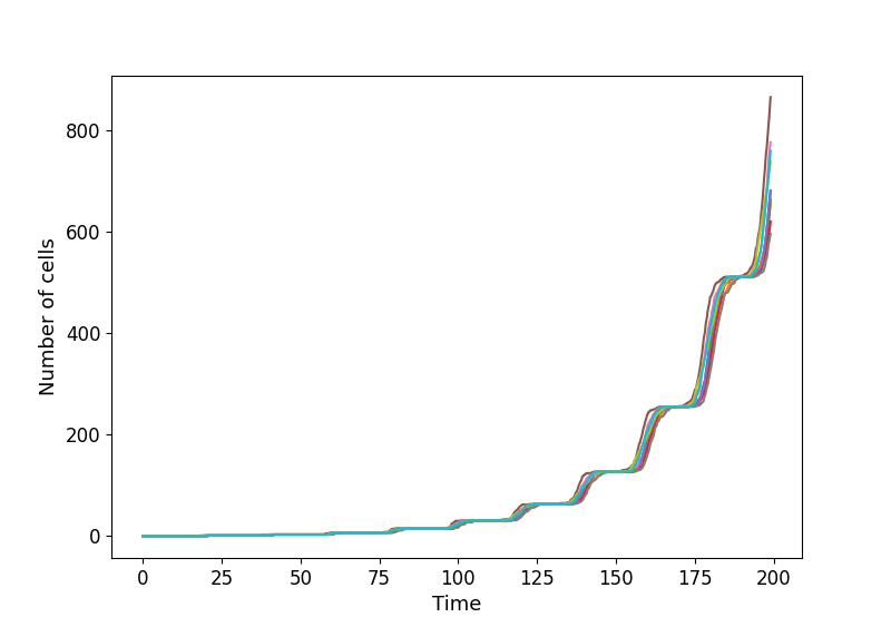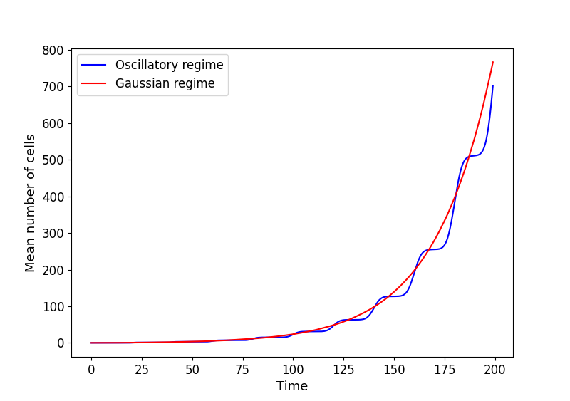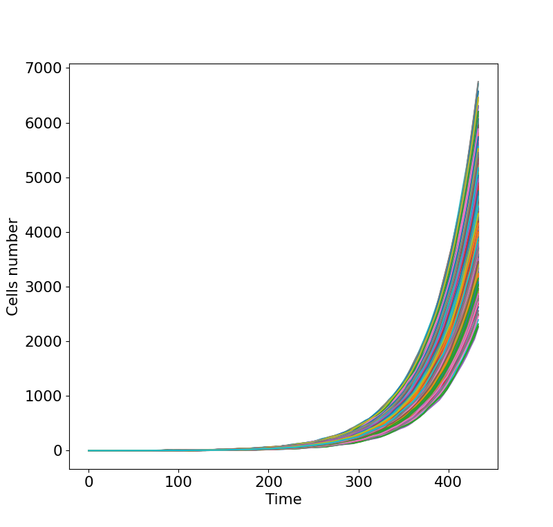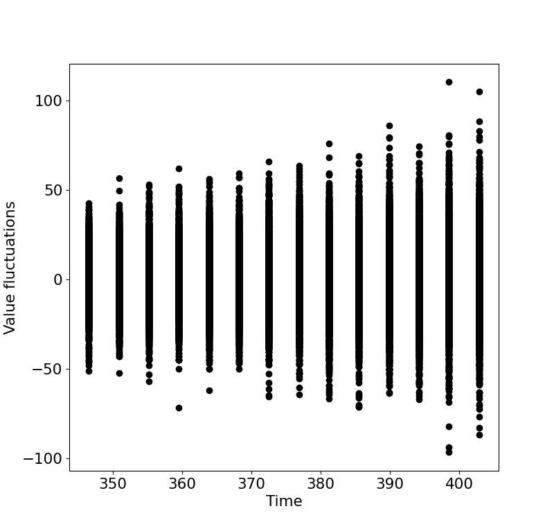The renormalized process has then asymptotically deterministic oscillations along time. These oscillations are due to the lack of variability in division times, implying too much synchronicity in the division times (see Figure 2). These oscillations involve a non-Gaussian, finite and complex random variable $M_{\delta}$ and the time step $\delta$:

(4) $$\frac{R_{t}^{\delta}}{\exp(\lambda t)}-2|M_{\delta}|\cos(\tau t+\arg(M_{\delta}))\overset{\mathbb{P}}{\underset{t\longrightarrow+\infty}{\longrightarrow}}0,$$

where

(5) $$\lambda=\frac{2^{\frac{1}{k}}\cos\left(\frac{2\pi}{k}\right)-1}{\theta}>\alpha/2,\qquad\tau=\frac{2^{\frac{1}{k}}\sin\left(\frac{2\pi}{k}\right)}{\theta}.$$

This classification in two regimes involving the spectral gap is known for multitype processes from the works of Athreya [3, 4]. In our study, the key ingredient is the asymptotic behavior of $Y_{t}^{\delta}=\mathbb{E}(N_{t+\delta}|\mathcal{F}_{t})-e^{\delta\alpha}\,N_{t}$, where $(\mathcal{F}_{t})_{t\geq 0}$ is the filtration of the process. For Bellman-Harris processes, in the Gaussian regime, it has been obtained in [22]. We add then the Gaussian contribution of $X_{t}^{\delta}=N_{t+\delta}-\mathbb{E}(N_{t+\delta}|\mathcal{F}_{t})$, which is at the same order of magnitude and asymptotically independent. This yields the long time behavior of $R_{t}^{\delta}=X_{t}^{\delta}+Y_{t}^{\delta}$ and the expression of the variance of the limiting Gaussian law $\sigma_{\delta}^{2}$. For the oscillating and non-Gaussian regime, we use recent and fine results of [21] to get the asymptotic behavior of $Y_{t}^{\delta}$. The second contribution $X_{t}^{\delta}$ still behaves with Gaussian fluctuations of order $\sqrt{N_{t}}$ but is now negligible.

We then exploit these results to infer the value of the parameters $(k,\theta)$ from the observations of $R_{t}^{\delta}$. The initial step is to discern which of the two regimes, (3) or (4), we find ourselves. This can be achieved by quantifying the order of magnitude of $R_{t}^{\delta}$. For this step, one has to be careful to the time parameter $\delta$, since $|M_{\delta}|$ vanishes for some values of $\delta$, see Section 3.1. The other difficulty comes from identifiability of the parameters since in the Gaussian regime, the limiting variance $\sigma_{\delta}^{2}$ is not injective with respect to the parameter $k$. We propose a procedure for the estimation which take into account these issues. We evaluate our method by using simulations, respectively in Sections 3.2 and 3.3 for the Gaussian regime (3) and the oscillating regime or (4). We recover in any case the parameters of the lifetime from the population size at given times and study the speed of convergence. This shows the efficiency of our procedure in our setting. Finally, in Section 4, we use our approach for inference on two data set. This allows to estimate the heterogeneity for the cell division time from monitoring at the population level, which is our original motivation for this work.

2. Regimes of asymptotic fluctuations

To present the different regimes of convergence of the fluctuations, we need to introduce some notations. Recall that $k\in[1,\infty)$ and $\theta\in(0,\infty)$ are fixed and $g(t)=t^{k-1}\exp(-\frac{t}{\theta})/({\Gamma(k)\theta^{k}})$ is the density of the Gamma law. We restrict ourselves to the Gamma distribution with $k\geq 1$, because the case where $k<1$ concerns distributions whose standard deviation is greater than the mean, and is therefore not relevant to our motivation. We introduce the cumulative distribution function $G$, and the Laplace transform $\mathcal{L}g$ related to our distribution,

$$G(a)=\int_{0}^{a}g(s)ds,\qquad\mathcal{L}g(\rho)=\int_{0}^{+\infty}g(u)e^{-\rho u}du=\frac{1}{(1+p\theta)^{k}},$$

for respectively $a\geq 0$, and $\rho\in\mathbb{C}$ such that $Re(\rho)>-1/\theta$. With an abuse of notation, for all $\rho\in\mathbb{C}\backslash\{-1/\theta\}$ such that $Re(\rho)\leq-1/\theta$, we also denote $\mathcal{L}g(\rho)=1/(1+p\theta)^{k}$ the analytic continuation of $\mathcal{L}g$. Finally, we introduce the stationary age distribution

$$p(a)=\frac{e^{-\alpha a}(1-G(a))}{\int_{0}^{\infty}e^{-\alpha u}(1-G(u))du},$$

and refer to [5] for the details of the proof. The Bellman-Harris process is defined inductively by starting from an initial number of individuals $N_{0}\in\mathbb{N}^{*}$ and initial ages $(A_{i})_{i=1,\ldots N_{0}}$. The individuals live during random times, which are independent and distributed as a Gamma law $\Gamma(k,\theta)$. At the end of their life, they are replaced by two individuals with age $0$. When we start from one single individual with age $a\in\mathbb{R}_{+}$, we denote by $\mathbb{E}_{a}$ and $\text{Var}_{a}$ the associated expectation and the associated variance. Unless otherwise specified, we start from one single individual with age $0$.

We now give the different regimes of approximations of the fluctuations. The result holds for a Bellman-Harris process starting from one individual with age $0$. Classical arguments for branching processes enable the extension of the results to more general initial conditions.

Theorem 1.

Consider a Bellman-Harris $N$ where the lifespan of individuals is distributed as $\zeta\sim\Gamma(k,\theta)$, with $k\geq 1,\theta>0$. The following statements hold.

1. If $2\cos\left(\frac{2\pi}{k}\right)<2^{-\frac{1}{k}}+1$, then for any $\delta>0$,

   $$\frac{R_{t}^{\delta}}{\sqrt{N_{t}}}\overset{\mathcal{L}}{\underset{t\longrightarrow+\infty}{\Longrightarrow}}\mathcal{N}\left(0,\sigma_{\delta}^{2}\right),$$

   where

   $$\sigma_{\delta}^{2} =\int_{\mathbb{R}^{+}}\emph{Var}_{a}(N_{\delta})p(a)da+2\alpha\int_{\mathbb{R}_{+}}\emph{Var}\Big{(}j^{(\delta)}(x)1_{[0,\zeta[}(x)$$

   $$\qquad\qquad+2h^{(\delta)}(x-\zeta)1_{[\zeta,+\infty[}(x)\Big{)}e^{-\alpha\,x}dx$$

   and for any $x\geq 0$ the functions

   $$j^{(\delta)}(x)=\mathbb{E}_{x}\left[N_{\delta}\right]-e^{\alpha\delta},\text{ and }h^{(\delta)}(x)=\mathbb{E}\left[N_{x+\delta}\right]-e^{\alpha\delta}\mathbb{E}\left[N_{x}\right].$$

2. If $2\cos\left(\frac{2\pi}{k}\right)=2^{-\frac{1}{k}}+1$, then for any $\delta>0$,

   $$\frac{R_{t}^{\delta}}{\sqrt{tN_{t}}}\overset{\mathcal{L}}{\underset{t\longrightarrow+\infty}{\Longrightarrow}}\mathcal{N}\left(0,{\sigma_{\delta}}^{2}\right),$$

   where

   $$\sigma_{\delta}^{2}=\frac{\alpha}{k^{2}}\frac{2^{\frac{2}{k}}}{2^{\frac{2}{k}}-2^{\frac{1}{k}}}\left|e^{(\lambda+i\tau)\delta}-e^{\alpha\delta}\right|^{2}.$$

3. If $2\cos\left(\frac{2\pi}{k}\right)>2^{-\frac{1}{k}}+1$, then for any $\delta>0$,

   $$\left|\frac{R_{t}^{\delta}}{\exp\left(\lambda t\right)}-2\left|M_{\delta}\right|\cos\left[\tau t+\arg\left(M_{\delta}\right)\right]\right|\overset{\mathbb{P}}{\underset{t\longrightarrow+\infty}{\longrightarrow}}0,$$

   where

   $$M_{\delta}=\left(e^{(\lambda+i\tau)\delta}-e^{\alpha\delta}\right)M,$$

   and $M$ is a complex random variable that does not depend on $\delta$.

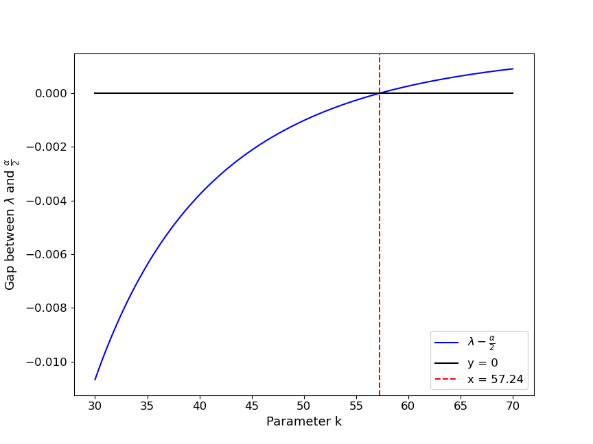
This theorem shows that two different regimes may be observed, excluding the very specific critical behavior. They depend on the value of $k$ and correspond respectively to a Gaussian regime, with the expected order of magnitude $\sqrt{N_{t}}$, and an oscillatory regime. The threshold value $k_{c}$ between these two regimes is given by

(6) $$\cos\left(\frac{2\pi}{k_{c}}\right)=\frac{1}{2}\left(2^{-\frac{1}{k_{c}}}+1\right),$$

and is approximately $57.24$, as illustrated in Figure 1.

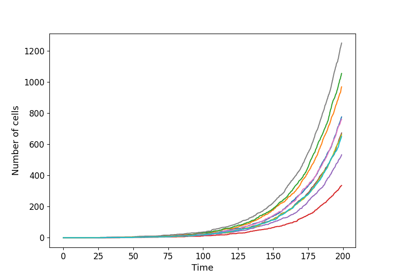
Recalling that $k=1/(\sigma/\mu)^{2}$, the threshold $k_{c}$ is equivalent to a coefficient of variation $\sigma/\mu$ of approximately $0.1322$. The oscillating regime (Theorem 1 $iii)$) then corresponds to a small variability of the lifespan, making the convergence to the age profile slow, while a large coefficient of variation helps for mixing and leads to the Gaussian regime (Theorem 1 $i)$). We illustrate this in Figure 2.

Figure 1. Curve of $\lambda-\frac{\alpha}{2}$ versus the parameter $k$ for $\theta=1$.

(a) Ten dynamics in the oscillatory regime. This corresponds to the parameters $\left(k,\theta\right)=(400,0.05)$.

(b) Ten dynamics in the Gaussian regime. This corresponds to the parameters $\left(k,\theta\right)=\left(6.25,3.38\right)$.

(c) Mean of the evolution of $500$ Bellman-dynamics in both regime. Done with the parameters given in $(a)$ and $(b)$.

Figure 2. Illustration of the two regimes, for parameters with the same Malthusian coefficient.

We prove now Theorem 1 by splitting $R_{t}^{\delta}$ in two parts. At each time $t$, we can label the individuals by $i=1,\ldots,N_{t}$ and we denote by $N_{t,\delta}^{i}$ the number of offspring of individual $i$ at time $t+\delta$. We introduce

$$R_{t}^{\delta}=X_{t}^{\delta}+Y_{t}^{\delta},$$

where

(7) $$X_{t}^{\delta} =N_{t+\delta}-\mathbb{E}(N_{t+\delta}|\mathcal{F}_{t})=\sum_{i=1}^{N_{t}}\left(N_{t,\delta}^{i}-\mathbb{E}(N_{t,\delta}^{i}|\mathcal{F}_{t})\right),$$

$$Y_{t}^{\delta} =\mathbb{E}(N_{t+\delta}|\mathcal{F}_{t})-e^{\delta\alpha}\,N_{t}=\sum_{i=1}^{N_{t}}\left(\mathbb{E}(N_{t,\delta}^{i}|\mathcal{F}_{t})-e^{\alpha\delta}\right).$$

The result in [21] applied to a suitable functional would allow to deal directly with $R_{t}^{\delta}$ but the decomposition $R_{t}^{\delta}=X_{t}^{\delta}+Y_{t}^{\delta}$ is interesting for itself. It yields two asymptotically independent contributions, which provide a natural expression of the limiting variance.

2.1. Asymptotic behavior of $X_{t}^{\delta}$

Let us study the asymptotic behavior of $(X_{t}^{\delta})_{t\geq 0}$ for all $\delta>0$. We first remark by (7) that for all $t\geq 0$ and $\delta>0$, the quantity $X_{t}^{\delta}$ can be seen as the sum of $N_{t}$ variables that are centered and independent conditionally with respect to $\mathcal{F}_{t}$. Thus, a slight adaptation of the central limit theorem allows to obtain the asymptotic behavior of $(X_{t}^{\delta})_{t\geq 0}$. To do so, we need the following upper bounds and regularity for the moments of $N_{\delta}$.

Lemma 1.

For any $\delta>0$, the following statements hold.

1. $\sup_{a\in[0,\infty)}\left\{\mathbb{E}_{a}[N_{\delta}^{2}]+\mathbb{E}_{a}\left[|N_{\delta}-\mathbb{E}_{a}[N_{\delta}]|^{3}|\right]\right\}<\infty$.

2. The function $a\mapsto\mathbb{E}_{a}\left[N_{\delta}\right]$ is continuous.

3. The function $a\mapsto\mathbb{E}_{a}\left[N_{\delta}^{2}\right]$ is continuous.

Note that $i)$ implies that the first moment and variance of $N_{\delta}$ are bounded with respect to the age $a$ of the root at time $0$, for any fixed time $\delta>0$. This bound is natural : a large age accelerates the first reproduction but in any case, we have then two individuals with age $0$.

Proof.

Let us first prove $i)$ and let $a\geq 0$. We consider a Bellman-Harris process $(N_{t})_{t\geq 0}$ starting from one single individual with age $a$. Then, the first time of division is the Gamma law with parameters $(k,\theta)$ conditioned to be larger than $a$ and its density is $g(a+x)/(1-G(a))$ for $x\geq 0$. Using an integral equation ([20, Theo. $15.1$] or [16, Eq. $7.1$]), we obtain

(8) $$\mathbb{E}_{a}[N_{\delta}] =2I_{\delta}(a)+\frac{1-G(a+\delta)}{1-G(a)},\quad\text{where }\,I_{\delta}(a)=\int_{0}^{\delta}\mathbb{E}_{0}[N_{\delta-x}]\frac{g(a+x)}{1-G(a)}dx.$$

Moreover, using [20, Theorem $18.1$]), we have

(9) $$\mathbb{E}_{a}[N_{\delta}^{2}]=\int_{0}^{\delta}\mathbb{E}\left[\left(\overline{N}_{\delta-x}^{(1)}+\overline{N}_{\delta-x}^{(2)}\right)^{2}\right]\frac{g(a+x)}{1-G(a)}dx+\frac{1-G(a+\delta)}{1-G(a)},$$

where $(\overline{N}_{t}^{(1)})_{t\geq 0}$ and $(\overline{N}_{t}^{(2)})_{t\geq 0}$ are two independent Bellman-Harris processes starting from an age $0$. Then, using the inequality $(y+z)^{2}\leq 2y^{2}+2z^{2}$ for all $y,z\in\mathbb{R}$, and the increasing of $t\mapsto\mathbb{E}_{0}[(N_{t})^{2}]$, allows to conclude that

(10) $$\mathbb{E}_{a}[N_{\delta}^{2}]\leq 4\mathbb{E}_{0}[(N_{\delta})^{2}]+1.$$

Secondly, as $\mathbb{E}_{a}[N_{\delta}]\geq 0$ and $N_{\delta}\geq 0$ almost surely, we have

$$|N_{\delta}-\mathbb{E}_{a}[N_{\delta}]|^{3}\leq\max\left(|\mathbb{E}_{a}[N_{\delta}]|^{3},|N_{\delta}|^{3}\right)\hskip 4.2679pt\leq|N_{\delta}|^{3}+|\mathbb{E}_{a}[N_{\delta}]|^{3}\text{ almost surely}.$$

In view of (10), we easily have that $|\mathbb{E}_{a}[N_{\delta}]|^{3}\leq\left(4\mathbb{E}_{0}[(N_{\delta})^{2}]+1\right)^{\frac{3}{2}}$. Proceeding as when we obtain (10) allows to obtain that $\mathbb{E}_{a}\left[|N_{\delta}|^{3}\right]$ is bounded by a constant independent from $a$. These two statements combined with (10) imply that $i)$ is proved.

Now, for $ii)$, as $k\geq 1$, one can easily see that $||g||_{\infty}<+\infty$. Using (8) and the fact that $G$ is continuous, we only have to prove that $a\mapsto I_{\delta}(a)$ is continuous to obtain the continuity of $a\mapsto\mathbb{E}_{a}[N_{\delta}]$. It is easily shown by noticing that

$$\left|\mathbb{E}_{0}[N_{\delta-x}]g(a+x)1_{\{x\in[0,\delta]\}}\right|\leq||g||_{\infty}\mathbb{E}_{0}[N_{\delta}]1_{\{x\in[0,\delta]\}},$$

and that the right-hand side is integrable. This proves $ii)$.

The proof of $iii)$ is very similar. We use the integral equation (9), and then the following domination

$$\left|\mathbb{E}\left[\left(\overline{N}_{\delta-x}^{(1)}+\overline{N}_{\delta-x}^{(2)}\right)^{2}\right]g(a+x)1_{\{x\in[0,\delta]\}}\right|\leq 4||g||_{\infty}\mathbb{E}_{0}[(N_{\delta})^{2}]1_{\{x\in[0,\delta]\}}.$$

This completes the proof. ∎

With this lemma, we are able to obtain the asymptotic behavior of $(X_{t}^{\delta})_{t\geq 0}$ for all $\delta>0$ by adapting the proof of the central limit theorem. Let us do this through the following proposition.

Proposition 1.

For any $\delta>0$,

$$\mathbb{E}\left[\exp\left(is\frac{X_{t}^{\delta}}{\sqrt{N_{t}}}\right)\,\bigg{|}\,\mathcal{F}_{t}\right]\overset{a.s.}{\underset{t\longrightarrow+\infty}{\longrightarrow}}\exp\left(-\frac{\sigma_{X,\delta}^{2}s^{2}}{2}\right),$$

where $\sigma_{X,\delta}^{2}=\int_{\mathbb{R}^{+}}\emph{Var}_{a}(N_{\delta})\,p(a)\,da$.

Proof.

Let $t\geq 0,\,\delta>0$ and $j\in\llbracket 1,N_{t}\rrbracket$. We denote by $A_{t}^{j}$ the age of the individual $j$ at time $t$, i.e. the initial age of the process $N_{t,\delta}^{j}$. Besides, we introduce the random variables

$$Z_{t,\delta}^{j}=\frac{N_{t,\delta}^{j}-\mathbb{E}[N_{t,\delta}^{j}|\mathcal{F}_{t}]}{\sqrt{N_{t}}},\qquad\sigma_{t,j,\delta}^{2}=\text{Var}_{A_{t}^{j}}(N_{\delta}),$$

and for all $s\in\mathbb{R}$

$$\Delta_{t,\delta}^{j}(s)=e^{isZ_{t,\delta}^{j}}-\left(1+isZ_{t,\delta}^{j}-\frac{s^{2}(Z_{t,\delta}^{j})^{2}}{2}\right),\hskip 2.84526ptD_{t,\delta}^{j}(s)=\exp\left(-\frac{s^{2}\sigma_{t,j,\delta}^{2}}{2N_{t}}\right)-\left(1-\frac{s^{2}\sigma_{t,j,\delta}^{2}}{2N_{t}}\right).$$

As $\mathbb{E}\left[Z_{t,\delta}^{j}|\mathcal{F}_{t}\right]=0$ and $\mathbb{E}\left[(Z_{t,\delta}^{j})^{2}|\mathcal{F}_{t}\right]=\frac{\sigma_{t,j,\delta}^{2}}{N_{t}}$, we have for all $s\in\mathbb{R}$

$$\left|\mathbb{E}[e^{isZ_{t,\delta}^{j}}|\mathcal{F}_{t}]-\exp\left(-\frac{s^{2}\sigma_{t,j,\delta}^{2}}{2N_{t}}\right)\right| =\left|\mathbb{E}[\Delta_{t,\delta}^{j}(s)|\mathcal{F}_{t}]-D_{t,\delta}^{j}(s)\right|$$

$$\leq|\mathbb{E}[\Delta_{t,\delta}^{j}(s)|\mathcal{F}_{t}]|+|D_{t,\delta}^{j}(s)|.$$

We use now the classical inequalities (see [6, Lemma 10.1.5,p.320], we adapt easily this lemma for $e^{-y}$) for $x\in\mathbb{R}$, $y\in\mathbb{R}_{+}$, $n\geq 1$

$$\left|e^{ix}-\sum_{j=0}^{n}\frac{(ix)^{j}}{j!}\right|\leq\frac{|x|^{n+1}}{(n+1)!},\hskip 28.45274pt\left|e^{-y}-\sum_{j=0}^{n}\frac{(-y)^{j}}{j!}\right|\leq\frac{|y|^{n+1}}{(n+1)!},$$

to obtain for all $s\in\mathbb{R}$

$$\left|\mathbb{E}[e^{isZ_{t,\delta}^{j}}|\mathcal{F}_{t}]-\exp\left(-\frac{s^{2}\sigma_{t,j,\delta}^{2}}{2N_{t}}\right)\right| \leq\mathbb{E}\left[\frac{\left|sZ_{t,\delta}^{j}\right|^{3}}{6}|\mathcal{F}_{t}\right]+\frac{s^{4}\sigma_{t,j,\delta}^{4}}{8N_{t}^{2}}$$

$$=\frac{|s|^{3}}{6N_{t}^{\frac{3}{2}}}\mathbb{E}\left[|N_{t,\delta}^{j}-\mathbb{E}[N_{t,\delta}^{j}|\mathcal{F}_{t}]|^{3}|\mathcal{F}_{t}\right]+\frac{s^{4}\sigma_{t,j,\delta}^{4}}{8N_{t}^{2}}.$$

Finally, in view of Lemma 1, we have for all $s\in\mathbb{R}$ the following inequality

(11) $$\left|\mathbb{E}[e^{isZ_{t,\delta}^{j}}|\mathcal{F}_{t}]-\exp\left(-\frac{s^{2}\sigma_{t,j,\delta}^{2}}{2N_{t}}\right)\right| \leq\frac{|s|^{3}}{6N_{t}^{\frac{3}{2}}}\sup_{a\in[0,\infty)}\left\{\mathbb{E}_{a}\left[|N_{\delta}-\mathbb{E}_{a}[N_{\delta}]|^{3}|\right]\right\}$$

$$\qquad+\frac{s^{4}}{8N_{t}^{2}}\left(\sup_{a\in[0,\infty)}\left\{\mathbb{E}_{a}[N_{\delta}^{2}]\right\}\right)^{2}.$$

Moreover, by branching property and (7), we also have

$$\mathbb{E}\left[\exp\left(is\frac{X_{t}^{\delta}}{\sqrt{N_{t}}}\right)\,\bigg{|}\,\mathcal{F}_{t}\right]=\prod_{j=1}^{N_{t}}\mathbb{E}\left[\exp\left(isZ_{t,\delta}^{j}\right)|\mathcal{F}_{t}\right].$$

Then, using the inequality $|\prod_{j=1}^{p}x_{j}-\prod_{j=1}^{p}y_{j}|\leq\sum_{i=1}^{p}|x_{j}-y_{j}|$ for $p\in\mathbb{N}^{*}$, $(x_{j})_{1\leq j\leq p}$ and $(y_{j})_{1\leq j\leq p}$ sequences of complex numbers such that for all $j\in\llbracket 1,p\rrbracket$ $|x_{j}|,|y_{j}|\leq 1$, and then using Equation (11), imply that almost surely

(12) $$\left|\mathbb{E}\left[\exp\left(is\frac{X_{t}^{\delta}}{\sqrt{N_{t}}}\right)\,\bigg{|}\,\mathcal{F}_{t}\right]-\exp\left(-\frac{s^{2}}{2N_{t}}\sum_{j=1}^{N_{t}}\text{Var}_{A_{j}}(N_{\delta})\right)\right|$$

$$\qquad\leq\sum_{j=1}^{N_{t}}\left|\mathbb{E}\left[\exp\left(isZ_{t,\delta}^{j}\right)|\mathcal{F}_{t}\right]-\exp\left(-\frac{s^{2}\text{Var}_{A_{j}}(N_{\delta})}{2N_{t}}\right)\right|$$

$$\qquad\leq\frac{|s|^{3}}{6N_{t}^{\frac{1}{2}}}\sup_{a\in[0,\infty)}\left\{\mathbb{E}_{a}\left[|N_{\delta}-\mathbb{E}_{a}[N_{\delta}]|^{3}|\right]\right\}+\frac{s^{4}}{8N_{t}}\left(\sup_{a\in[0,\infty)}\left\{\mathbb{E}_{a}[N_{\delta}^{2}]\right\}\right)^{2}.$$

The right-hand side goes to $0$ almost surely as $t$ tends to infinity, using Lemma 1 and that $N_{t}$ tends to infinity. In addition, all the statements of Lemma 1 imply that the function $x\mapsto\text{Var}_{x}(N_{\delta})$ is bounded continuous. Then, by [5, Corollary 3] we have

$$\frac{s^{2}}{2N_{t}}\sum_{j=1}^{N_{t}}\text{Var}_{A_{j}}(N_{\delta})~{}\overset{a.s.}{\underset{t\longrightarrow+\infty}{\longrightarrow}}~{}\frac{s^{2}}{2}\sigma_{X,\delta}^{2}.$$

The latter combined with (12) through a triangular inequality ends the proof. ∎

One can easily check that this proposition implies

$$\frac{X_{t}^{\delta}}{\sqrt{N_{t}}}{\underset{t\longrightarrow+\infty}{\Longrightarrow}}\mathcal{N}\left(0,\sigma_{X,\delta}^{2}\right).$$

We keep the convergence of the process conditionally with respect to $(\mathcal{F}_{t})_{t\geq 0}$ to be able to combine the convergence of $(X_{t}^{\delta})_{t\geq 0}$ with the convergence of $(Y_{t}^{\delta})_{t\geq 0}$.

2.2. Asymptotic behavior of $Y_{t}^{\delta}$

Let us focus now on the asymptotic behavior of $(Y_{t}^{\delta})_{t\geq 0}$ for all $\delta>0$. By Equation (7), we see that for all $t\geq 0$, $\delta>0$, similar to $X_{t}^{\delta}$, the random variable $Y_{t}^{\delta}$ can be seen as the sum of $N_{t}$ independent random variables. To obtain the behavior of $(Y_{t}^{\delta})_{t\geq 0}$, we use the result in [21] which deals with more general processes. Some preliminaries are required to use this result. Let us give these in the following lemma.

Lemma 2.

Let us suppose that $k\geq 1$, $\theta>0$. Then for any $\delta>0$, the following statements hold.

1. The function $h_{1}(a)=\mathbb{E}_{a}[N_{\delta}]$ is continuously differentiable on $(0,\infty)$, and there exists $C_{h_{1}}>0$ such that for all $a>0$

   (13) $$|h^{\prime}_{1}(a)|\leq C_{h_{1}}\left(a^{k-2}1_{a<1}+1\right).$$

2. There exists $C_{h_{2}}>0$ such that for $h_{2}(a)=\left(\mathbb{E}_{a}\left[N_{\delta}\right]-e^{\alpha\delta}\right)\left(1-G(a)\right)1_{\{a\geq 0\}}$, we have

   $$\emph{V}h_{2}(a)\leq C_{h_{2}}.1_{\{a\geq 0\}}\left(1+\min(a,1)^{k-1}+a\right),$$

   where $\emph{V}f$ is defined for any function $f$ by

   $$\emph{V}f(x)=\sup\left\{\sum_{j=1}^{n}|f(x_{j})-f(x_{j-1})|\,\big{|}\,-\infty<x_{0}<x_{1}<\ldots<x_{n}\leq x,\,n\in\mathbb{N}\right\}.$$

3. The function $h_{3}(a)=e^{-\alpha\,a}\left((1-G(a))-(1-G(a))^{2}\right)\left(\mathbb{E}_{a}\left[N_{\delta}\right]-e^{\alpha\delta}\right)^{2}$ is directly Riemann integrable on $[0,\infty)$, i.e.

   $$\sum_{n\geq 0}\underset{y\in(n\epsilon,(n+1)\epsilon]}{\sup}f(y)<+\infty,\quad\text{ and }\quad\epsilon\sum_{n\geq 0}\big{\{}\underset{(n\epsilon,(n+1)\epsilon]}{\sup}f(y)-\underset{(n\epsilon,(n+1)\epsilon]}{\inf}f\big{\}}\underset{\epsilon\longrightarrow 0}{\longrightarrow}0.$$

Proof.

Let us first prove $i)$. By (8), as $G$ is continuously differentiable, we only have to prove that $a\mapsto I_{\delta}(a)$ is continuously differentiable on $(0,+\infty)$. As $g^{\prime}(y){\longrightarrow}0$ when $y{\longrightarrow}\infty$, and $g^{\prime}$ is continuous on $(0,+\infty)$, we have for all $\eta>0$ that $\sup_{[\eta,+\infty)}|g^{\prime}|<+\infty$. The continuous differentiability of $a\mapsto I_{\delta}(a)$ then follows from the following integrable bound, for $a\in[\eta,+\infty)$,

$$\left|\mathbb{E}_{0}[N_{\delta-x}]g^{\prime}(a+x)1_{\{x\in[0,\delta]\}}\right|\leq\sup_{y\in[\eta,+\infty)}|g^{\prime}(y)|\mathbb{E}_{0}[N_{\delta}]1_{\{x\in[0,\delta]\}}.$$

Let us prove now (13). By (8), for all $a>0$

$$h_{1}^{\prime}(a) =2\frac{\partial}{\partial a}I_{\delta}(a)+\frac{\partial}{\partial a}\frac{1-G(a+\delta)}{1-G(a)}$$

$$=2\int_{0}^{\delta}\mathbb{E}_{0}[N_{\delta-x}]\left(\frac{g^{\prime}(a+x)}{1-G(a)}+\frac{g(a+x)g(a)}{(1-G(a))^{2}}\right)dx+\frac{(1-G(a+\delta))g(a)}{(1-G(a))^{2}}-\frac{g(a+\delta)}{1-G(a)}.$$

Then, using the fact that $G$ increases, we have for all $a>0$

(14) $$\left|h_{1}^{\prime}(a)\right| \leq 2\mathbb{E}_{0}[N_{\delta}]\int_{0}^{\delta}\left(\left|\frac{g^{\prime}(a+x)}{1-G(a)}\right|+\frac{g(a+x)g(a)}{(1-G(a+x))(1-G(a))}\right)dx$$

$$\qquad+\frac{g(a)}{1-G(a)}+\frac{g(a+\delta)}{1-G(a+\delta)}.$$

To continue, we need upper bounds for $s\mapsto\frac{g(s)}{1-G(s)}$ and $s\mapsto\sup_{x\geq 0}\left|\frac{g^{\prime}(s+x)}{1-G(s)}\right|$. First, by L’Hôpital’s rule we have

$$\lim_{a\longrightarrow+\infty}\frac{g(a)}{1-G(a)}=-\lim_{a\longrightarrow+\infty}\frac{g^{\prime}(a)}{g(a)}=-\lim_{a\longrightarrow+\infty}(\log(g(a)))^{\prime}=\frac{1}{\theta}.$$

The latter combined with the fact that $g$ and $G$ are continuous yields

(15) $$\sup_{s\geq 0}\frac{g(s)}{1-G(s)}<+\infty.$$

Second, for all $(x,a)\in[0,\delta]\times(0,+\infty)$, we have by using triangular inequality, and the fact that $G$ increases

$$\left|\frac{g^{\prime}(a+x)}{1-G(a)}\right| =\left|\frac{k-1}{a+x}\frac{g(a+x)}{1-G(a)}-\frac{g(a+x)}{\left(1-G(a)\right)\theta}\right|$$

$$\leq\frac{k-1}{a+x}\frac{g(a+x)}{1-G(1)}1_{\{a\leq 1\}}+\left((k-1)1_{\{a>1\}}+\frac{1}{\theta}\right)\frac{g(a+x)}{1-G(a+x)}.$$

Using the fact that when $k\geq 2$ we have

$$\frac{g(a+x)}{a+x}1_{\{a\leq 1\}}\leq\frac{(a+x)^{k-2}}{\Gamma(k)\theta^{k}}1_{\{a\leq 1\}}\leq\frac{(1+\delta)^{k-2}}{\Gamma(k)\theta^{k}}1_{\{a\leq 1\}},$$

and when $1\leq k<2$ we have

$$\frac{g(a+x)}{a+x}1_{\{a\leq 1\}}\leq\frac{a^{k-2}}{\Gamma(k)\theta^{k}}1_{\{a\leq 1\}},$$

we obtain

(16) $$\left|\frac{g^{\prime}(a+x)}{1-G(a)}\right| \leq\frac{k-1}{(1-G(1))\Gamma(k)\theta^{k}}\left((1+\delta)^{k-2}+a^{k-2}\right)1_{\{a\leq 1\}}$$

$$+\left((k-1)1_{\{a>1\}}+\frac{1}{\theta}\right)\sup_{s\geq 0}\frac{g(s)}{1-G(s)}.$$

Then, plugging (15) and (16) in (14) yields (13).

Let us turn to the proof of $ii)$. The function $h_{2}(a)=\left(\mathbb{E}_{a}\left[N_{\delta}\right]-e^{\alpha\delta}\right)\left(1-G(a)\right)1_{\{a\geq 0\}}$ is continuously differentiable on $(0,+\infty)$ by $i)$, and with zero derivatives on $(-\infty,0)$. Moreover, we easily have that $|h_{2}(0^{-})-h_{2}(0)|=h_{2}(0)$, and by continuity $|h_{2}(0^{+})-h_{2}(0)|=0$ (see Lemma 1 $ii)$). Therefore, using the expression of the total variation for a piecewise continuously differentiable function yields for all $a\in\mathbb{R}$

(17) $$\emph{V}h_{2}(a)=\begin{cases}0,&\text{ for }a<0,\\ |h_{2}(0)|+\int_{0}^{a}\left|h^{\prime}_{2}(s)\right|ds,&\text{ for }a\geq 0.\end{cases}$$

For all $s>0$, we have using a triangular inequality, and then Lemmas 1 and 2

$$|h^{\prime}_{2}(s)| =\left|h^{\prime}_{1}(s)(1-G(s))-g(s)\left(\mathbb{E}_{s}\left[N_{\delta}\right]-e^{\alpha\delta}\right)\right|$$

$$\leq C_{h_{1}}\left(s^{k-2}1_{s<1}+1\right)+||g||_{\infty}\left(\sup_{y\geq 0}\left(\mathbb{E}_{y}\left[N_{\delta}\right]\right)+e^{\alpha\delta}\right).$$

Plugging this in (17) yields $ii)$.

Finally, by Lemma 1 $i)$, we easily obtain that there exists a constant $K>0$ such that for all $a\geq 0$,

$$h_{3}(a)=e^{-\alpha a}\left((1-G(a))-(1-G(a))^{2}\right)\left(\mathbb{E}_{a}\left[N_{\delta}\right]-e^{\alpha\delta}\right)^{2}\leq Ke^{-\alpha a}.$$

By [2, Prop. $4.1.$V,$p.154$], $a\mapsto Ke^{-\alpha a}$ is directly Riemann integrable as this is a non-increasing Lebesgue integrable function. Then, $h_{3}$ is directly Riemann integrable by [2, Prop. $4.1.$IV,$p.154$], as it is a bounded continuous function (Lemma 1), dominated by $a\mapsto Ke^{-\alpha a}$. ∎

Thus, we have all the auxiliary statements we need to apply the result in [21]. We now introduce some notations linked to this article. We use [21] and consider for all $t\geq 0,\delta>0$

$$\Delta_{t}^{\delta}=Y_{t}^{\delta}-\sum_{\begin{subarray}{c}\rho\in\mathbb{C}\backslash\{-1/\theta\},\\ \mathcal{L}g(\rho)=\frac{1}{2},\text{Re}(\rho)>\frac{\alpha}{2}\end{subarray}}e^{\rho\,t}\frac{\int_{\mathbb{R}}h_{2}(x)e^{-\rho\,x}dx}{2\int_{0}^{+\infty}xe^{-\rho x}g(x)dx}W(\rho),$$

where $h_{2}$ has been defined in Lemma 2, and $W(\rho)$ is the limit almost surely and in $L^{2}$ of the martingale $(W_{t}(\rho))_{t\geq 0}$ defined in [21, Eq. $2.17$]. We do not explicit the latter as this requires introducing too many notations. For all $\delta>0$, we can obtain the asymptotic behavior of $(\Delta_{t}^{\delta})_{t\geq 0}$ by using [21, Theorem $2.8$]. This theorem gives the ergodic behavior for $(\Delta_{t}^{\delta})_{t\geq 0}$, as the cost of a renormalization that is different according to the fact that the set $\{\rho\in\mathbb{C}\backslash\{-1/\theta\}:\mathcal{L}g(\rho)=1/2,\text{Re}(\rho)=\alpha/2\}$ is empty or not. The second case corresponds in fact to a critical case, when the spectral gap $\alpha-\lambda=\frac{\alpha}{2}$. Let us give the asymptotic behavior of $(\Delta_{t}^{\delta})_{t\geq 0}$ for all $\delta>0$ in the following proposition.

Proposition 2.

Let $\delta>0$. Then there exists $\sigma_{Y,\delta}^{2}$ such that

$$t^{b}e^{-\alpha t/2}\Delta_{t}^{\delta}\,\left(1,\frac{1}{\sqrt{W}}\right)\,\overset{\mathcal{L}}{\underset{t\longrightarrow+\infty}{\Longrightarrow}}\,\mathcal{N}(0,\sigma_{Y,\delta}^{2})\left(\sqrt{\frac{W}{\beta}},\frac{1}{\sqrt{\beta}}\right),$$

where $\mathcal{N}(0,\sigma_{Y,\delta}^{2})$ is a centered Gaussian random variable with variance $\sigma_{Y,\delta}^{2}$ independent of $W$, $\beta=2\int_{0}^{\infty}ug(u)e^{-\alpha u}du$, and

$$b=\begin{cases}0,&\text{if }\left\{\rho\in\mathbb{C}\backslash\{-1/\theta\}:\mathcal{L}g(\rho)=1/2,\text{Re}(\rho)=\alpha/2\right\}=\varnothing,\\ -1/2,&\text{otherwise.}\end{cases}$$

Proof.

Let $\delta>0$. Bellman-Harris processes are a special class of Crump-Mode-Jagers processes where the reproduction happens only at the end of the life of each individual. We can thus apply Theorem $2.8$ in [21], which deals with Crump-Mode-Jagers processes with random characteristic, by checking the assumptions of this result, namely $(A1-A3)$, $(A5-A6)$ and $(2.19)$ (the density of the intensity measure with respect to the Lebesgue measure is immediate). In our case, the reproduction point process of the Crump-Mode-Jagers process is $\xi=\sum_{j=1}^{2}\delta_{\zeta}$, and the random characteristic is

$$\varphi(x)=\left(\mathbb{E}_{x}\left[N_{\delta}\right]-e^{\alpha\delta}\right)1_{[0,\zeta[}(x),$$

where $\zeta\sim\Gamma(k,\theta).$

As $\mathcal{L}g(\alpha)=\frac{1}{2}$ and $-\left(\mathcal{L}g\right)^{\prime}(\alpha)=\int_{0}^{+\infty}xe^{-\alpha x}g(x)dx>0$, Assumption $(A1)$ of [21] is satisfied. Moreover, the reproduction law is reduced to binary division, so Assumptions $(A2)$ and $(A3)$ of [21] are directly satisfied (see Remark $2.1$ of [21]).
Noticing that for all $a\in\mathbb{R}$, $e^{-\alpha a}\text{Var}(\varphi(a))=h_{3}(a)1_{a\geq 0}$, and using Lemma 2 $iii)$ imply that $(A5)$ is satisfied.
Let $t\in\mathbb{R}$ and $\epsilon=1$. By Lemma 1 $i)$, notice that for all $x\in\mathbb{R}$,

$$\left|\varphi(x)\right|\leq\left(\sup_{s\geq 0}\mathbb{E}_{s}\left[N_{\delta}\right]+e^{\alpha\delta}\right)<+\infty.$$

Thus the family $\left(|\varphi(x)|^{2}\right)_{x\in[t-\epsilon,t+\epsilon]}$ is bounded and $(A6)$ is satisfied.
Equation $(2.19)$ in [21] is satisfied by using Lemma 2 $ii)$, and the fact that for all $c>0$

$$\int_{0}^{\infty}\left(1+\min(x,1)^{k-1}+x\right)(e^{-cx}+e^{-\alpha x})dx<+\infty.$$

In addition, for all $p\in\mathbb{C}$ such that $Re(p)\neq\frac{1}{\theta}$ we have

(18) $$(\mathcal{L}g)^{\prime}(p)=-\frac{k\theta}{(1+p\theta)^{k+1}}\neq 0.$$

Then, every root of $p\mapsto\mathcal{L}g(p)-\frac{1}{2}$ is a root of multiplicity $1$. We have now checked the assumptions of [21, Theorem $2.8$] and get the convergence in law of $t^{b}e^{-\alpha t/2}\Delta_{t}^{\delta}$. Adding that this convergence is stable by [21, Remark $2.13$], and that $W>0$ a.s. by [5, Theo. $2$ , $p.172$], ends the proof of the convergence in law of the bivariate random variable.
∎

The previous proposition shows that the asymptotic behavior of $(Y_{t}^{\delta})_{t\geq 0}$ depends on the set $\{\rho\in\mathbb{C}\backslash\{-1/\theta\}:\mathcal{L}g(\rho)=1/2\}$. In our case, with Gamma distribution of lifespan, this set is explicit. Indeed, for all $p\in\mathbb{C}$ such that $p\neq-\frac{1}{\theta}$, we have

(19) $$\mathcal{L}g(p)=\frac{1}{(1+p\theta)^{k}}.$$

We can solve this equation and obtain

(20) $$\left\{\rho\in\mathbb{C}\backslash\{-1/\theta\}:\mathcal{L}g(\rho)=\frac{1}{2}\right\}=\left\{\frac{2^{\frac{1}{k}}\exp\left(\frac{2\pi\,l}{k}i\right)-1}{\theta}\,|\,l\in\left\llbracket-\left\lceil\frac{k}{2}\right\rceil+1,\left\lfloor\frac{k}{2}\right\rfloor\right\rrbracket\right\}.$$

Recalling the expressions of $\alpha,\lambda,\tau$ from (5), we derive that when $k\geq 2$

$$\alpha,\,\lambda\pm i\tau\in\,\left\{\rho\in\mathbb{C}\backslash\{-1/\theta\}:\mathcal{L}g(\rho)=1/2\right\},$$

and when $k\in[1,2)$

(21) $$\left\{\rho\in\mathbb{C}\backslash\{-1/\theta\}:\mathcal{L}g(\rho)=1/2\right\}=\{\alpha\}.$$

We can now classify the convergence of $(Y_{t}^{\delta})_{t\geq 0}$ and explain the cases of Theorem 1.

Proposition 3.

Let $\delta>0$. The following result of convergence holds.

1. If $2\cos\left(\frac{2\pi}{k}\right)<2^{-\frac{1}{k}}+1$, then

   $$\frac{Y_{t}^{\delta}}{\sqrt{N_{t}}}\overset{\mathcal{L}}{\underset{t\longrightarrow+\infty}{\Longrightarrow}}\mathcal{N}\left(0,2\alpha\sigma_{Y,\delta}^{2}\right),$$

   where

   $$\sigma_{Y,\delta}^{2}=\int_{\mathbb{R}_{+}}\emph{Var}\left(\left(\mathbb{E}_{x}\left[N_{\delta}\right]-e^{\alpha\delta}\right)1_{[0,\zeta[}(x)+2h^{(\delta)}(x-\zeta)1_{[\zeta,+\infty[}(x)\right)e^{-\alpha\,x}dx.$$

2. If $2\cos\left(\frac{2\pi}{k}\right)=2^{-\frac{1}{k}}+1$, then

   $$\frac{Y_{t}^{\delta}}{\sqrt{tN_{t}}}\overset{\mathcal{L}}{\underset{t\longrightarrow+\infty}{\Longrightarrow}}\mathcal{N}\left(0,2\alpha\sigma_{Y,\delta}^{2}\right),$$

   where

   $$\sigma_{Y,\delta}^{2}=\frac{1}{2k^{2}}\frac{2^{\frac{2}{k}}}{2^{\frac{2}{k}}-2^{\frac{1}{k}}}\left|e^{(\lambda+i\tau)\delta}-e^{\alpha\delta}\right|^{2}.$$

3. If $2\cos\left(\frac{2\pi}{k}\right)>2^{-\frac{1}{k}}+1$, then

   $$\left|\frac{Y_{t}^{\delta}}{\exp\left(\lambda t\right)}-2\left|M_{\delta}\right|\cos\left[\tau t+\arg\left(M_{\delta}\right)\right]\right|\overset{\mathbb{P}}{\underset{t\longrightarrow+\infty}{\longrightarrow}}0,$$

   where

   $$M_{\delta}=\left(e^{(\lambda+i\tau)\delta}-e^{\alpha\delta}\right)M,$$

   and $M$ is complex random variable that does not depend on $\delta$.

Proof.

We prove $i)$. First, by (20), we notice that when $k\geq 2$

$$\lambda=\max\left\{Re(\rho):\rho\in\mathbb{C}\backslash\{-1/\theta,\alpha\},\,\mathcal{L}g(\rho)=1/2\right\}.$$

Then, the latter and (21) imply that in the case $2\cos\left(\frac{2\pi}{k}\right)<2^{-\frac{1}{k}}+1$, which is equivalent to $\lambda<\alpha/2$, we have

(22) $$\left\{\rho\in\mathbb{C}\backslash\{-1/\theta\}:\mathcal{L}g(\rho)=\frac{1}{2},Re(\rho)\geq\frac{\alpha}{2}\right\} =\{\alpha\}.$$

Second, following the proof of Proposition 2 allows to check the Assumptions of [21, Lemma $7.6$] for the random characteristics $\varphi_{1}(x)=1_{[0,\zeta[}(x)$ and $\varphi_{2}(x)=\mathbb{E}_{x}[N_{\delta}]1_{[0,\zeta[}(x)$, where $\zeta\sim\Gamma(k,\theta)$. This result ensures that there exists $c\in(0,\frac{\alpha}{2})$ such that

$$\mathbb{E}\left[N_{t+\delta}\right]=\sum_{\begin{subarray}{c}\rho\in\mathbb{C}\backslash\{-1/\theta\},\\ \mathcal{L}g(\rho)=\frac{1}{2},\text{Re}(\rho)\geq\frac{\alpha}{2}\end{subarray}}\frac{\int_{0}^{+\infty}e^{-\rho\,x}(1-G(x))dx}{2\int_{0}^{+\infty}xe^{-\rho\,x}g(x)dx}e^{\rho(t+\delta)}+O\left(e^{c\,t}\right),$$

and

$$\mathbb{E}\left[N_{t+\delta}\right] =\mathbb{E}\left[\sum_{j=1}^{N_{t}}\mathbb{E}[N_{t,\delta}^{j}|\mathcal{F}_{t}]\right]$$

$$=\sum_{\begin{subarray}{c}\rho\in\mathbb{C}\backslash\{-1/\theta\},\\ \mathcal{L}g(\rho)=\frac{1}{2},\text{Re}(\rho)\geq\frac{\alpha}{2}\end{subarray}}\frac{\int_{0}^{+\infty}e^{-\rho\,x}\mathbb{E}_{x}\left[N_{\delta}\right](1-G(x))dx}{2\int_{0}^{+\infty}xe^{-\rho\,x}g(x)dx}e^{\rho\,t}+O\left(e^{c\,t}\right).$$

By identifying the coefficients of these two expansions, we get

(23) $$\int_{0}^{+\infty}\mathbb{E}_{x}\left[N_{\delta}\right]e^{-\alpha\,x}(1-G(x))dx =e^{\alpha\delta}\int_{0}^{+\infty}e^{-\alpha\,x}(1-G(x))dx,$$

and finally

(24) $$\int_{0}^{+\infty}h_{2}(x)e^{-\alpha x}dx=0.$$

Combining this equation with (22) implies that for all $t\geq 0$, $\delta>0$,

(25) $$\Delta_{t}^{\delta}=Y_{t}^{\delta}.$$

Combining now Equations (22) and (25), and Proposition 2, we get

$$e^{-\alpha t/2}\,{W}^{-1/2}\,Y_{t}^{\delta}\,\overset{\mathcal{L}}{\underset{t\longrightarrow+\infty}{\Longrightarrow}}\,\frac{1}{\sqrt{\beta}}\mathcal{N}(0,\sigma_{Y,\delta}^{2}).$$

We also know that

$$\sqrt{N_{t}}\,{W}^{-1/2}\,e^{-\alpha t/2}\overset{a.s.}{\underset{t\longrightarrow+\infty}{\longrightarrow}}\sqrt{n_{1}},$$

where $n_{1}=\frac{1}{2\alpha\beta}$, see [20, Theo. $21.1$, $p.147$]. Combining these two results of convergence through Slutsky’s lemma allows to obtain the convergence. We mention that we can also obtain this convergence by applying [22, Corollary 2], but this only works when the parameter $k$ of the Gamma distribution is an integer.
To know the value of $\sigma_{Y,\delta}^{2}$ when $2\cos\left(\frac{2\pi}{k}\right)<2^{-\frac{1}{k}}+1$, we use the expression given in [21, Theorem $2.14$]. We are in the case where $n=-1$ (as $p\mapsto\mathcal{L}g(p)-\frac{1}{2}$ has no roots such that $Re(p)=\alpha/2$). Then, if we consider $\zeta\sim\Gamma(k,\theta)$, and if we denote for all $y\in\mathbb{R}$ the function $h^{(\delta)}(y)=(\mathbb{E}\left[N_{y+\delta}\right]-e^{\alpha\delta}\mathbb{E}\left[N_{y}\right])1_{[0,\infty[}(y)$, we have by [21, Theorem $2.14$] that

(26) $$\sigma_{Y,\delta}^{2} =\int_{\mathbb{R}}\text{Var}(\varphi(x)+2h^{(\delta)}(x-\zeta)1_{[\zeta,+\infty[}(x))e^{-\alpha\,x}dx$$

$$=\int_{\mathbb{R}_{+}}\text{Var}\left(\left(\mathbb{E}_{x}\left[N_{\delta}\right]-e^{\alpha\delta}\right)1_{[0,\zeta[}(x)+2h^{(\delta)}(x-\zeta)1_{[\zeta,+\infty[}(x)\right)e^{-\alpha\,x}dx.$$

We prove now $ii)$. As $\lambda=\max\left\{Re(\rho)\,|\,2.\mathcal{L}g(\rho)=1\right\}$, we have by the condition of the statement and (20) that

(27) $$\left\{\rho\in\mathbb{C}\backslash\{-1/\theta\}:\mathcal{L}g(\rho)=\frac{1}{2},\,Re(\rho)>\frac{\alpha}{2}\right\} =\{\alpha\},$$

$$\left\{\rho\in\mathbb{C}\backslash\{-1/\theta\}:\mathcal{L}g(\rho)=\frac{1}{2},\,Re(\rho)=\frac{\alpha}{2}\right\} =\left\{\lambda-i\tau,\lambda+i\tau\right\}.$$

We prove similarly to the previous point that (23) is satisfied, implying that for all $t\geq 0$, $\delta>0$, we have $\Delta_{t}^{\delta}=Y_{t}^{\delta}$. Then, by Proposition 2 $ii)$,

$$t^{-1/2}e^{-\alpha t/2}\left(\sqrt{W}\right)^{-1}Y_{t}^{\delta}\,\overset{\mathcal{L}}{\underset{t\longrightarrow+\infty}{\Longrightarrow}}\,\frac{1}{\sqrt{\beta}}\mathcal{N}(0,\sigma_{Y,\delta}^{2}).$$

Using (1) and Slutsky’s lemma, we can switch from $W$ to $N_{t}$ in this convergence and get $ii).$
We now compute $\sigma_{Y,\delta}^{2}$ when $2\cos\left(\frac{2\pi}{k}\right)=2^{-\frac{1}{k}}+1$. It is direct that if we consider $\zeta\sim\Gamma(k,\theta)$ we have by the expression of the variance given in [21, Theorem $2.14$] (we are in the case where $n=0$, as the roots of $p\mapsto\mathcal{L}g(p)-\frac{1}{2}$ such that $Re(p)=\alpha/2$ have a multiplicity $1$)

$$\sigma_{Y,\delta}^{2}=\sum_{\begin{subarray}{c}\rho\in\mathbb{C}\backslash\{-1/\theta\},\\ \mathcal{L}g(\rho)=\frac{1}{2},\,Re(\rho)=\frac{\alpha}{2}\end{subarray}}\text{Var}\left[\left(\frac{e^{\rho\delta}-e^{\alpha\delta}}{2\rho\int_{0}^{+\infty}xe^{-\rho\,x}g(x)dx}\right)e^{-\rho\,\zeta}\right].$$

As for a complex random variable $Z$ and a constant $c\in\mathbb{C}$ we have $\text{Var}(cZ)=\mathbb{E}[|cZ|^{2}]-\left|\mathbb{E}[cZ]\right|^{2}=|c|^{2}\text{Var}(Z)$, and as $\left\{\rho\in\mathbb{C}\backslash\{-1/\theta\},\,2.\mathcal{L}g(\rho)=1,\,Re(\rho)=\frac{\alpha}{2}\right\}=\{\lambda-i\tau,\lambda+i\tau\}$, we obtain

$$\sigma_{Y,\delta}^{2} =\sum_{s\in\{-1,1\}}\left|\frac{e^{(\lambda+is\tau)\delta}-e^{\alpha\delta}}{2(\lambda+is\tau)\int_{0}^{+\infty}xe^{-(\lambda+is\tau)\,x}g(x)dx}\right|^{2}\text{Var}\left[e^{-(\lambda+is\tau)\zeta}\right].$$

As $\mathbb{E}\left[e^{-\alpha\zeta\,}\right]=\mathcal{L}g(\alpha)=1/2$, as for the same reason $\mathbb{E}\left[e^{-(\lambda+i\tau)\zeta\,}\right]=\mathbb{E}\left[e^{-(\lambda-i\tau)\zeta\,}\right]=1/2$, and as $\alpha=2\lambda$, we have $\text{Var}\left[e^{-(\lambda\pm i\tau)\zeta}\right]=\mathbb{E}\left[e^{-2\lambda\zeta}\right]-\left|\mathbb{E}\left[e^{-(\lambda\pm i\tau)\zeta}\right]\right|^{2}=1/2-1/4=1/4$. Plugging this in the above equation yields

$$\sigma_{Y,\delta}^{2} =\frac{1}{4}\left|\frac{e^{(\lambda+i\tau)\delta}-e^{\alpha\delta}}{2(\lambda+i\tau)\int_{0}^{+\infty}xe^{-(\lambda+i\tau)\,x}g(x)dx}\right|^{2}+\frac{1}{4}\left|\frac{e^{(\lambda-i\tau)\delta}-e^{\alpha\delta}}{2(\lambda-i\tau)\int_{0}^{+\infty}xe^{-(\lambda-i\tau)\,x}g(x)dx}\right|^{2}.$$

Using the fact that $\int_{0}^{+\infty}xe^{-(\lambda\pm i\tau)\,x}g(x)dx=-\mathcal{L}^{\prime}(g)(\lambda\pm i\lambda)$, Equation (18), the fact that $1/[1+(\lambda\pm i\tau)\theta]^{k}=\mathcal{L}g(\lambda\pm i\tau)=\frac{1}{2}$, and finally the equality $2\cos\left(\frac{2\pi}{k}\right)=2^{-\frac{1}{k}}+1$, we get

$$\sigma_{Y,\delta}^{2} =\frac{1}{4}\left|\frac{1}{k}\frac{2^{\frac{1}{k}}\exp\left(i\frac{2\pi}{k}\right)}{2^{\frac{1}{k}}\exp\left(i\frac{2\pi}{k}\right)-1}\right|^{2}\left[\left|\left(e^{(\lambda+i\tau)\delta}-e^{\alpha\delta}\right)\right|^{2}+\left|e^{(\lambda-i\tau)\delta}-e^{\alpha\delta}\right|^{2}\right]$$

$$=\frac{1}{2k^{2}}\frac{2^{\frac{2}{k}}}{2^{\frac{2}{k}}+1-2^{\frac{1}{k}+1}\cos\left(\frac{2\pi}{k}\right)}\left|e^{(\lambda+i\tau)\delta}-e^{\alpha\delta}\right|^{2}$$

$$=\frac{1}{2k^{2}}\frac{2^{\frac{2}{k}}}{2^{\frac{2}{k}}-2^{\frac{1}{k}}}\left|e^{(\lambda+i\tau)\delta}-e^{\alpha\delta}\right|^{2}.$$

We finally prove $iii)$. In this case,

$$\lambda=\max\left\{Re(\rho):\rho\in\mathbb{C}\backslash\{-1/\theta,\alpha\},\,\mathcal{L}g(\rho)=1/2\right\}\in(\alpha/2,\alpha).$$

Moreover, one can prove as in the first point that (23) and (24) are true. Then, we have the following equality for all $t\geq 0$, $\delta>0$

(28) $$\frac{Y_{t}^{\delta}}{\exp\left(\lambda t\right)}-\sum_{\begin{subarray}{c}\rho\in\mathbb{C}\backslash\{-1/\theta\},\\ \mathcal{L}g(\rho)=\frac{1}{2},\text{Re}(\rho)=\lambda\end{subarray}}e^{(\rho-\lambda)t}\frac{\int_{\mathbb{R}}h_{2}(x)e^{-\rho\,x}dx}{2\int_{0}^{+\infty}xe^{-\rho x}g(x)dx}W(\rho)$$

$$=\frac{\Delta_{t}^{\delta}}{\exp\left(\lambda t\right)}+\sum_{\begin{subarray}{c}\rho\in\mathbb{C}\backslash\{-1/\theta\},\\ \mathcal{L}g(\rho)=\frac{1}{2},\lambda>\text{Re}(\rho)>\alpha/2\end{subarray}}e^{(\rho-\lambda)t}\frac{\int_{\mathbb{R}}h_{2}(x)e^{-\rho\,x}dx}{2\int_{0}^{+\infty}xe^{-\rho x}g(x)dx}W(\rho).$$

As $\lambda>\alpha/2$, by Proposition 2 (whatever the case) and Slutsky’s lemma we have

(29) $$\frac{\Delta_{t}^{\delta}}{\exp\left(\lambda t\right)}\overset{\mathcal{L}}{\underset{t\longrightarrow+\infty}{\Longrightarrow}}0.$$

We also easily have that

(30) $$\sum_{\begin{subarray}{c}\rho\in\mathbb{C}\backslash\{-1/\theta\},\\ \mathcal{L}g(\rho)=\frac{1}{2},\lambda>\text{Re}(\rho)>\alpha/2\end{subarray}}e^{(\rho-\lambda)t}\frac{\int_{\mathbb{R}}h_{2}(x)e^{-\rho\,x}dx}{2\int_{0}^{+\infty}xe^{-\rho x}g(x)dx}W(\rho)\overset{a.s.}{\underset{t\longrightarrow+\infty}{\longrightarrow}}0.$$

Combining (29) and (30) through Slutsky’s lemma yields

(31) $$\frac{Y_{t}^{\delta}}{\exp\left(\lambda t\right)}-\sum_{\begin{subarray}{c}\rho\in\mathbb{C}\backslash\{-1/\theta\},\\ \mathcal{L}g(\rho)=\frac{1}{2},\text{Re}(\rho)=\lambda\end{subarray}}e^{(\rho-\lambda)t}\frac{\int_{\mathbb{R}}h_{2}(x)e^{-\rho\,x}dx}{2\int_{0}^{+\infty}xe^{-\rho x}g(x)dx}W(\rho)\overset{\mathcal{L}}{\underset{t\longrightarrow+\infty}{\Longrightarrow}}0.$$

We know by (20) that $\{\rho\in\mathbb{C}\backslash\{-1/\theta\}:\mathcal{L}g(\rho)=\frac{1}{2},\text{Re}(\rho)=\lambda\}=\left\{\lambda-i\tau,\lambda+i\tau\right\}$. Proceeding as in the first point for (23), we can obtain that

$$\int_{0}^{+\infty}\mathbb{E}_{x}\left[N_{\delta}\right]e^{-(\lambda\pm i\tau)x}(1-G(x))dx =e^{(\lambda\pm i\tau)\delta}\int_{0}^{+\infty}e^{-(\lambda\pm i\tau)x}(1-G(x))dx$$

$$=\frac{e^{(\lambda\pm i\tau)\delta}}{\lambda\pm i\tau}\int_{0}^{+\infty}\left(1-e^{-(\lambda\pm i\tau)y}\right)g(y)dy=\frac{e^{(\lambda\pm i\tau)\delta}}{2(\lambda\pm i\tau)},$$

and more generally

(32) $$\int_{\mathbb{R}}h_{2}(x)e^{-(\lambda+i\tau)x}dx=\frac{e^{(\lambda+i\tau)\delta}-e^{\alpha\delta}}{2(\lambda+i\tau)}=\overline{\int_{\mathbb{R}}h_{2}(x)e^{-(\lambda-i\tau)x}dx}.$$

By (18), we also have that

(33) $$\int_{0}^{+\infty}xe^{-(\lambda+i\tau)x}g(x)dx=\overline{\int_{0}^{+\infty}xe^{-(\lambda-i\tau)x}g(x)dx}=-(\mathcal{L}g)^{\prime}(\lambda+i\tau)=\frac{k\theta}{2^{1+\frac{1}{k}}\exp\left(\frac{2\pi}{k}i\right)}.$$

As $W(\lambda+i\tau)$ and $W(\lambda-i\tau)$ are limits of conjugated martingales (see [21, Eq. $2.17$] for the expression of the martingale), we have that

(34) $$W(\lambda+i\tau)=\overline{W(\lambda-i\tau)}.$$

Plugging (32), (33) and (34) in (31) and using the equality $z+\overline{z}=2|z|\cos(\arg(z))$ yields that the statement of the proposition is proved for $M=\frac{1}{2k}\frac{2^{\frac{1}{k}}\exp\left(\frac{2\pi}{k}i\right)}{2^{\frac{1}{k}}\exp\left(\frac{2\pi}{k}i\right)-1}W(\lambda+i\tau).$ ∎

It remains now to combine Propositions 1 and 3 to obtain the asymptotic behavior of $(R_{t}^{\delta})_{t\geq 0}$ for all $\delta>0$.

2.3. Proof of Theorem 1

Proof of i).

Let $\delta>0$, $t\geq 0$. As $R_{t}^{\delta}=X_{t}^{\delta}+Y_{t}^{\delta}$ and $Y_{t}^{\delta}$ is $\mathcal{F}_{t}-$measurable, conditioning with respect to $\mathcal{F}_{t}$ yields

$$\mathbb{E}\left[e^{isR_{t}^{\delta}/\sqrt{N_{t}}}\right] =\mathbb{E}\left[\mathbb{E}\left[e^{isX_{t}^{\delta}/\sqrt{N_{t}}}\bigg{|}\mathcal{F}_{t}\right]e^{isY_{t}^{\delta}/\sqrt{N_{t}}}\right].$$

Then, using the triangular inequality and the fact that $|\exp(i.x)|=1$ for $x\in\mathbb{R}$ and $\sigma_{\delta}^{2}=\sigma_{X,\delta}^{2}+\sigma_{Y,\delta}^{2}$, we get

(35) $$\left|\mathbb{E}\left[e^{isR_{t}^{\delta}/\sqrt{N_{t}}}\right]-e^{-\sigma_{\delta}^{2}s^{2}/2}\right| \leq\mathbb{E}\left[\left|\mathbb{E}\left[e^{isX_{t}^{\delta}/\sqrt{N_{t}}}\bigg{|}\mathcal{F}_{t}\right]-e^{-\sigma_{X,\delta}^{2}s^{2}/2}\right|\right]$$

$$\qquad+e^{-\sigma_{X,\delta}^{2}s^{2}/2}\left|\mathbb{E}\left[e^{isY_{t}^{\delta}/\sqrt{N_{t}}}\right]-e^{-\sigma_{Y,\delta}^{2}s^{2}/2}\right|.$$

By Proposition 1 and the dominated convergence theorem, we have

$$\mathbb{E}\left[\left|\mathbb{E}\left[e^{isX_{t}^{\delta}/\sqrt{N_{t}}}\bigg{|}\mathcal{F}_{t}\right]-e^{-\sigma_{X,\delta}^{2}s^{2}/2}\right|\right]\underset{t\longrightarrow+\infty}{\longrightarrow}0.$$

By Proposition 3 and the Levy’s theorem, we also have

$$\left|\mathbb{E}\left[e^{isY_{t}^{\delta}/\sqrt{N_{t}}}\right]-e^{-\sigma_{Y,\delta}^{2}s^{2}/2}\right|\underset{t\longrightarrow+\infty}{\longrightarrow}0.$$

Plugging these two results of convergence in (35) implies that $i)$ is proved. ∎

Proof of ii).

By Proposition 1 and Slutsky’s lemma, $X_{t}^{\delta}/\sqrt{tN_{t}}$ converges to $0$ in law and thus in probability, as $t$ tends to infinity. By Proposition 3, $Y_{t}^{\delta}/\sqrt{tN_{t}}$ converges in law to a centered Gaussian variable with variance $2\alpha\sigma_{Y,\delta}^{2}$. Adding these two convergences with Slutsky’s lemma ends the proof of $ii)$. ∎

Proof of iii).

In the case $iii)$, $\lambda>\alpha/2$ and Proposition 1 ensures that $X_{t}^{\delta}\exp\left(-\lambda t\right)$ converges to $0$ in law and thus in probability, as $t$ tends to infinity. Besides, Proposition 3 $iii)$ ensures that $Y_{t}^{\delta}\exp\left(-\lambda t\right)$ converges in probability to $2\left|M_{\delta}\right|\cos\left[\tau t+\arg\left(M_{\delta}\right)\right]$. Adding these two limits yields the result. ∎

3. Estimation of the parameters from simulations

Let us use the results above on the asymptotic behavior of $(R_{t}^{\delta})_{t\geq 0}$ and propose an efficient way to infer the parameters $(k,\theta)$ of the lifespan. We assume that our data set consists in the observation of $n_{\text{data}}$ independent realizations of a Bellman-Harris with time distribution $\Gamma(k,\theta)$ at fixed instants of measures. We may forget the first times, when the population is small, since we rely on asymptotic analysis and are motivated by this framework. We may also discuss on the role of the times and choose the relevant set of times to exploit. The corresponding data set we use is then denoted by

$$(N_{i\Delta}^{(j)}:i\leq I,j\in\llbracket 1,n_{\text{data}}\rrbracket),$$

where $\Delta>0$, $I\in\mathbb{N}^{*}$.

We also need a numerical approximation of $\sigma_{\delta}^{2}$ introduced in Theorem 1 $i)$. The latter depends on the parameters $(k,\theta)$ of the lifetime distribution. Using the relation $\alpha~{}=~{}(2^{1/k}-1)/\theta$, we can also say that $\sigma_{\delta}^{2}$ depends on the values of $(k,\alpha)$. We prefer this viewpoint, as this is more relevant for our inference method. Thus, from now on, $\sigma_{\delta}^{2}$ refers to the function

$$\sigma_{\delta}^{2}:(k,\alpha)\in[1,k_{c})\times\mathbb{R}_{+}^{*}\mapsto\sigma_{\delta}(k,\alpha).$$

We denote $(k,\alpha)\mapsto\overline{\sigma}_{\delta}^{2}(k,\alpha)$ the approximation of $\sigma_{\delta}^{2}$. Let us explain how we compute it when $\alpha$ is fixed. We consider a grid of parameters

$$\mathbb{G}_{p}=\{1+pl\,|\,l\in\llbracket 0,\lfloor(k_{c}-1)/p\rfloor-1\rrbracket\},$$

where $p>0$. Then, for any $k\in\mathbb{G}_{p}$, we proceed by Monte Carlo simulations to approximate all the expectations and variances that compose $\sigma_{\delta}^{2}(k,\alpha)$, except those in function $h^{(\delta)}$. We refer to Section 6.1 to see how we approximate the latter. This gives us at the end an approximation $\overline{\sigma}_{\delta}^{2}(k,\alpha)$ of $\sigma_{\delta}^{2}(k,\alpha)$ for all $k\in\mathbb{G}_{p}$, that we extend to $k\geq 1$ using interpolation techniques.

To verify that this method works, we plot in Figure 3 the evolution of $\frac{R_{t,\delta}}{\sqrt{N_{t}}}$, for different sets of parameters, and see if the latter converges to a value close to $\overline{\sigma}_{\delta}^{2}$. We observe that this is the case. Thus, this approximation method seems good.

(a) $(k,\theta)=(18.75,0.8)$.

(b) $(k,\theta)=(28.9,0.59)$.

(c) $(k,\theta)=(35,1)$.

(d) $(k,\theta)=(46.8,2.1)$.

Figure 3. Comparison of $\overline{\sigma}_{\delta}^{2}$ with the variance of $\frac{R_{t,\delta}}{\sqrt{N_{t}}}$ in different cases. We use the grid of parameters $\mathbb{G}_{1/20}$, and we take $\delta$ as explained in Section 3.2.1. We also estimate the variance of $\frac{R_{t,\delta}}{\sqrt{N_{t}}}$ using the empirical estimator of the variance with $2000$ simulations of Bellman-Harris dynamics. To simplify the computation of $\overline{\sigma}_{\delta}^{2}$, we do the approximation that $\sigma_{\delta}^{2}$ does not depends on $\alpha$ (or equivalently $\theta$), see Figure 7(b) and the end of Section 3.2.1.

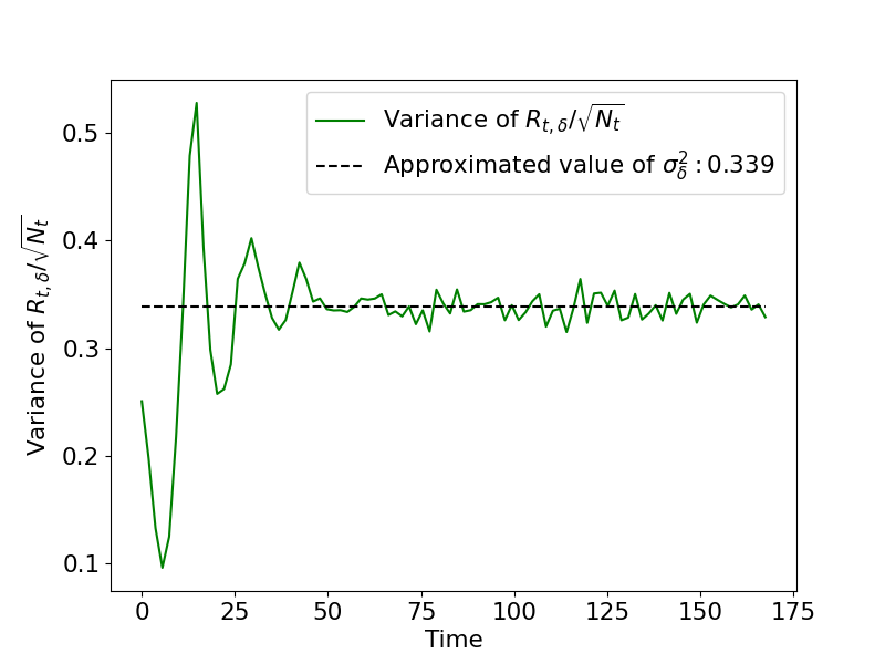
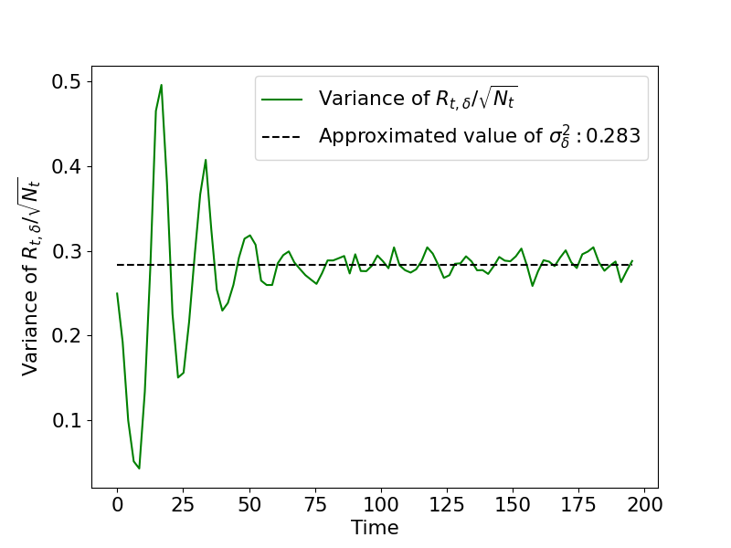
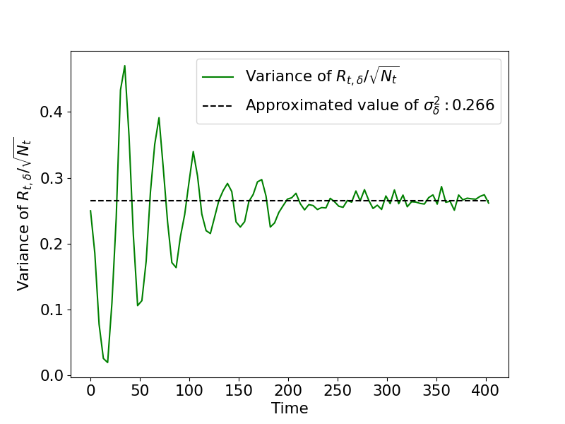
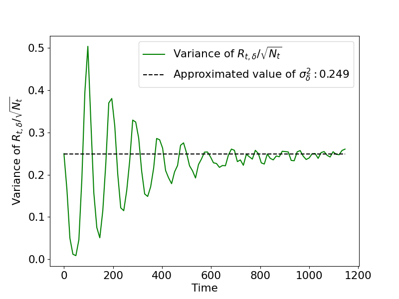
We now have everything we need to do the inference. We follow the following pipeline to recover $(k,\theta)$, and test it with simulations. In the rest of Section 3, the “number of simulations” is the number of dynamics we have simulated to create our dataset, so corresponds to $n_{\text{data}}$.

Step 1 : estimation $\widehat{\alpha}$ of the Malthusian coefficient $\alpha$. For all $j\in\llbracket 1,n_{\text{data}}\rrbracket$, we do a linear regression of $t\mapsto\log(N_{t}^{(j)})$ using our data set $(N_{i\Delta}^{(j)}:i\leq I)$, which gives us an estimated value $\widehat{\alpha}^{(j)}$. Then, we take

$$\widehat{\alpha}=\frac{1}{n_{\text{data}}}\sum_{i=1}^{n_{\text{data}}}\widehat{\alpha}^{(j)}$$

as an estimation of $\alpha$.

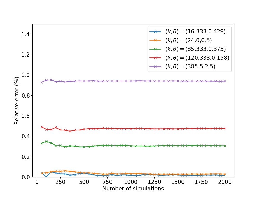
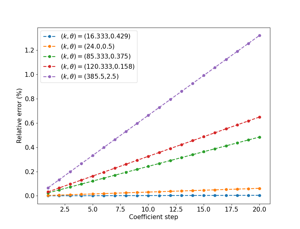
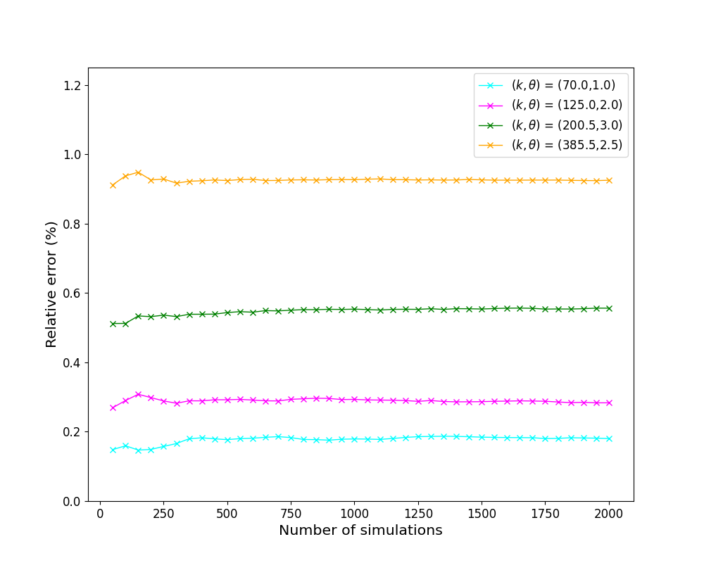
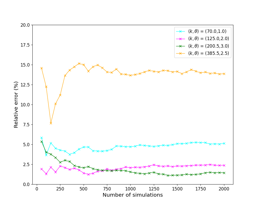
The estimation of $\alpha$ we obtain is very precise, even with a small number of simulations, as we see in Figure 4(a) where all the relative errors are below $1\%$. In addition, even exponential quantities such as $e^{\widehat{\alpha}\delta}$ closely approximate $e^{\alpha\delta}$. Indeed, we plot in Figure 4(b) the relative errors for the estimation of $e^{\alpha\delta}$, with $\delta$ of the order we choose in pratice (we refer to Sections 3.1.2 and 3.2.1), and we see that all the errors are below $1.5\%$.

(a) Relative error of the estimation of $\alpha$ versus the number or simulations, for a number of simulations in $\left\{50l\,|\,l\in\llbracket 1,40\rrbracket\right\}$.

(b) Relative error of the estimation of $e^{\alpha l\delta}$, with $\delta=\frac{\log(2)}{10\widehat{\alpha}}$, versus $l\in\llbracket 1,20\rrbracket$. The estimation was done using $100$ simulations.

Figure 4. Illustration of the estimation of $\alpha$ and $e^{\alpha\delta}$ for different parameters. Due to oscillations, see Figures 12(a) and 12(b), the errors slightly increase when $k$ increases.

Step 2 : determination of the (Gaussian or oscillating) regime. We assume here that we do not fall in the critical and need to determine from the data set if $2\cos\left(2\pi/k\right)-(2^{-1/k}+1)$ is positive or negative. For that purpose, we compare $\widehat{\alpha}$ with the growth of the empirical variance of $N_{t+\delta}-e^{\widehat{\alpha}\delta}N_{t}$

$$\widehat{\text{Var}}\left(N_{t+\delta}-e^{\widehat{\alpha}\delta_{1}}N_{t}\right)=\frac{1}{n_{\text{data}}}\sum_{k=1}^{n_{\text{data}}}\left(\left(N_{t+\delta}^{(k)}-e^{\widehat{\alpha}\delta}N_{t}^{(k)}\right)-\frac{1}{n_{\text{data}}}\sum_{j=1}^{n_{\text{data}}}\left(N_{t+\delta}^{(j)}-e^{\widehat{\alpha}\delta}N_{t}^{(j)}\right)\right)^{2},$$

where $t=i\Delta$, $i<I$. At this step, we need here to be careful in the choice of $\delta=\delta_{1}=n_{1}\Delta$, where $n_{1}\in\mathbb{N}^{*}$, see Section 3.1.

Step 3 : estimation $(\widehat{k},\widehat{\theta})$ of $(k,\theta)$. Recall that $\alpha$ has been estimated by $\widehat{\alpha}$. Depending on the regime, the estimator $(\widehat{k},\widehat{\theta})$ is different.
a) In the Gaussian regime, we consider the following estimators

(36) $$\widehat{k}=\underset{k\in[1,k_{c}[}{\text{argmin}}\left|\overline{\sigma_{\delta}}(k,\widehat{\alpha})^{2}-\frac{1}{n_{\text{times}}}\sum_{j=1}^{n_{\text{times}}}\widehat{\text{Var}}\left(N_{T_{j}+\delta}-e^{\widehat{\alpha}\delta}N_{T_{j}}\right)\right|,\text{ and }\widehat{\theta}=(2^{1/\widehat{k}}-1)/\widehat{\alpha},$$

where $n_{\text{times}}\in\llbracket 1,I\rrbracket$, and for all $j\in\llbracket 1,n_{\text{times}}\rrbracket$, $\left(T_{j}/\Delta,(T_{j}+\delta)/\Delta\right)\in\llbracket 0,I\rrbracket^{2}$. Here the time step $\delta=\delta_{2}=n_{2}\Delta$, where $n_{2}\in\mathbb{N}^{*}$, needs also to be chosen carefully to ensure uniqueness of the argmin. It will be different from $\delta_{1}$, see Sections 3.1 and 3.2.
b) In the oscillating regime, we first estimate $\lambda$ by $\widehat{\lambda}$ thanks to a linear regression : $\widehat{\lambda}$ is the slope of

$$t\mapsto\frac{1}{2}\log\left(\widehat{\text{Var}}\left(N_{t}-e^{\widehat{\alpha}\delta_{1}}N_{t}\right)\right).$$

Then, we estimate $(k,\theta)$ with

$$(\widehat{k},\widehat{\theta})=\underset{\begin{subarray}{c}(k,\theta)\in(k_{c},+\infty[\times\mathbb{R}_{+}^{*}\\ (2^{1/k}-1)/\theta=\widehat{\alpha}\end{subarray}}{\text{argmin}}\left|(2^{1/k}\cos\left(2\pi/k\right)-1)/\theta-\widehat{\lambda}\right|.$$

Let us now detail the main points of this procedure and give the results obtained by simulations. We first explain how to choose $\delta_{1}>0$ for the determination of the regime in Step $2$. Then, we consider the Gaussian regime and explain how to choose $\delta_{2}$ and compare in that case the estimated value to the theoretical one for simulations. We finally deal with the oscillating regime. The score we use to measure the quality of the estimation is the relative error, defined as

$$\text{relative error}=\frac{|\text{estimated value}-\text{theoric value}|}{\text{theoric value}}.$$

3.1. Determination of the regime

3.1.1. Why do we need to take care of the time step for the detection of the regime ?

Our approach relies on the study of

$$R_{T}^{\delta}=N_{T+\delta}-e^{\delta\alpha}\,N_{T}\,=X_{T}^{\delta}+Y_{T}^{\delta}.$$

Indeed, $R_{T}^{\delta}$ can be estimated from data, and is related to the parameters of interest $(k,\theta)$ in a sensible way. This link has been studied in Section 2. We have shown that when $\lambda>\alpha/2$, $X_{T}^{\delta}$ and $Y_{T}^{\delta}$ behave for large $T$ as follows

$$X_{T,\delta}\approx\mathcal{N}(0,\sigma_{X,\delta}^{2})\sqrt{n_{1}W}e^{T\alpha/2},\qquad Y_{T}^{\delta}\approx 2\left|M_{\delta}\right|\cos\left[\tau T+\arg\left(M_{\delta}\right)\right]e^{T\lambda}.$$

The Gaussian part $X_{T,\delta}$ then prevail compared to $Y_{T}^{\delta}$ when $T\rightarrow\infty$, see Theorem 1. We also recall that

$$M_{\delta}=f(\delta).M,\quad\text{with }f(\delta)=|e^{(\lambda+i\tau)\delta}-e^{\alpha\delta}|.$$

For applications, $T$ may not be very large. If $T\times(\lambda-\alpha/2)$ is positive but small, and $M_{\delta}$ is close to $0$, the two contributions $X_{T}^{\delta}$ and $Y_{T}^{\delta}$ may be comparable. In that case, it becomes difficult to detect that $\lambda-\alpha/2$ is positive and thus that we are in the oscillating regime. That’s why the choice of the time step $\delta$ matters, and we explain now how to avoid that $f(\delta)$ (and thus $M_{\delta}$) is too small.

3.1.2. Time step $\delta_{1}$ and detection of the regime.

Let us write $\delta=\delta(c)=c\log(2)/\alpha$, where $c>0$, and recall that

$$\alpha=\frac{2^{\frac{1}{k}}-1}{\theta},\qquad\lambda=\frac{2^{\frac{1}{k}}\cos\left(\frac{2\pi}{k}\right)-1}{\theta}>\alpha/2,\qquad\tau=\frac{2^{\frac{1}{k}}\sin\left(\frac{2\pi}{k}\right)}{\theta}.$$

We search a value of $c$ so that

$$f(\delta(c))=|e^{(\lambda+i\tau)c.\log(2)/\alpha}-e^{\alpha c.\log(2)/\alpha}|=|e^{(\lambda+i\tau)c.\log(2)/\alpha}-2^{c}|$$

is not to close to $0$. As we have

$$\lim_{k\rightarrow\infty}(\lambda+i\tau)\delta(c) =\lim_{k\rightarrow\infty}c\log(2)\left(\frac{2^{\frac{1}{k}}\cos\left(\frac{2\pi}{k}\right)-1}{\frac{1}{k}}+i\frac{2^{\frac{1}{k}}\sin\left(\frac{2\pi}{k}\right)}{\frac{1}{k}}\right)\frac{\frac{1}{k}}{2^{\frac{1}{k}}-1}$$

$$=c\left(\log(2)+i2\pi\right),$$

we obtain

$$\lim_{k\rightarrow\infty}f(\delta(c)) \,=\,2^{c}\sqrt{2\left(1-\cos\left(2\pi c\right)\right)}.$$

By this expression and the fact that the oscillating regime corresponds to large values of $k$, we see that the values of $c$ that seems interesting are those such that the cosines term is minimal, i.e. equal to $-1$. This corresponds to cases where $\delta=c\log(2)/\alpha$, with $c-1/2\in\mathbb{N}$. At the opposite, the values of $c$ that should be avoided are those such that the cosines term is maximal, i.e. equal to $1$, when $c\in\mathbb{N}^{*}$. To illustrate this, let us plot in Figure 5 the values of $f(\delta)=|e^{(\lambda+i\tau)\delta}-e^{\alpha\delta}|$ versus $\delta$, in the case where $(k,\theta)=(80.2,4)$.

Figure 5. Curve of $|e^{(\lambda+i\tau)\delta}-e^{\alpha\delta}|$ versus $\delta$, when $(k,\theta)=(80.2,4)$. Red lines represent multiples of $\log(2)/\alpha$.

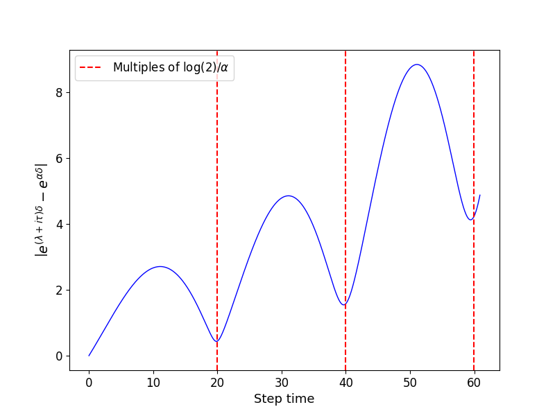
We see in Figure 5 that the value of the modulus is very low when $\delta$ is a multiple of $\log(2)/\alpha$. Then, choosing a step time that is a multiple of this value would imply bad results on the estimation of the regime.

At the opposite, in Figure 5, the amplitude of the oscillations seems to be maximal when $\delta=l\log(2)/\alpha+\log(2)/(2\alpha)$, where $l\in\mathbb{N}$. Then, it is better to take a time step as closed as possible of these values when we detect the regime. By default, we take the minimal step that satisfy this condition, that is

$$\delta_{1}=\underset{i\Delta,\,i\in\llbracket 0,I\rrbracket}{\text{argmin}}\left|\Delta i-\log(2)/(2\widehat{\alpha})\right|.$$

We take the minimal step because the error of the estimation of $e^{\alpha\delta}$ increases when $\delta$ increase, as observed in Figure 4(b).

3.1.3. The threshold for the detection

To detect the regime, we compare the slope of the linear regression of $t\mapsto\widehat{\text{Var}}\left(N_{t}-e^{\widehat{\alpha}\delta_{1}}N_{t}\right)$, which is $2\widehat{\lambda}$, to $\widehat{\alpha}$. Indeed, in the Gaussian regime, $\widehat{\lambda}$ does not estimate $\lambda$, but $\alpha/2$. In practice, we decide that we are in the Gaussian regime if the difference of these two terms is less than $10\%$ of $\widehat{\alpha}$. It is relevant in various cases, see the results in Sections 3.2.2 and 3.3. A more systemic exploration of the set of parameters or theoretical may be interesting and would allow to be more precise.

3.2. Inference in the Gaussian regime

3.2.1. Identifiability : the choice of the time step $\delta_{2}$ for the estimation

We need to choose the time step $\delta_{2}$ to achieve Step $3$. Our estimator (36) involves a minimization, and the problem is identifiable if there is a unique minimizer (argument of the minimum). This depends on the choice of $\delta$. Denoting $\widehat{\alpha}$ the estimator of $\alpha$, the uniqueness of the minimizer requires an injectivity property, for the function

$$k\mapsto\sigma_{\delta}^{2}(k,\widehat{\alpha})=\sigma_{X,\delta}^{2}(k,\widehat{\alpha})+2\widehat{\alpha}\sigma_{Y,\delta}^{2}(k,\widehat{\alpha}).$$

The function $\sigma_{\delta}^{2}(.,\widehat{\alpha})$ is not injective in general, as we see in Figure 6, where two different values of $k$ can have the same image by $\sigma_{\delta}^{2}(.,\widehat{\alpha})$. This comes from the fact that $\sigma_{X,\delta}^{2}(.,\widehat{\alpha})$ and $\sigma_{Y,\delta}^{2}(.,\widehat{\alpha})$ have opposite monotonicity.

(a) For $\delta=\log(2)/(2\widehat{\alpha})$.

(b) For $\delta=3\log(2)/(4\widehat{\alpha})$.

Figure 6. $\sigma_{\delta}^{2}(k,\widehat{\alpha})$ (black), $\sigma_{X,\delta}^{2}(k,\widehat{\alpha})$ (blue) and $2\widehat{\alpha}\sigma_{Y,\delta}^{2}(k,\widehat{\alpha})$ versus $k$, for $\widehat{\alpha}=1$, and for different time steps $\delta$ such that $\sigma_{\delta}^{2}(.,\widehat{\alpha})$ is not injective. $\sigma_{\delta}^{2}$ has been approximated using $\overline{\sigma}_{\delta}^{2}$, computed with the grid of parameters $\mathbb{G}_{1/2}$. The mesh size is small, because the non-smoothness of the curves when k is large decreases the readability of the figure with a larger mesh size. To approximate $\sigma_{X,\delta}^{2}$ and $\sigma_{Y,\delta}^{2}$, we only keep the part of our approximation of $\sigma_{\delta}^{2}$ that corresponds to each of these quantities.

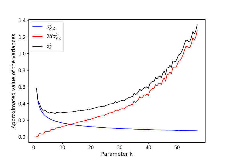
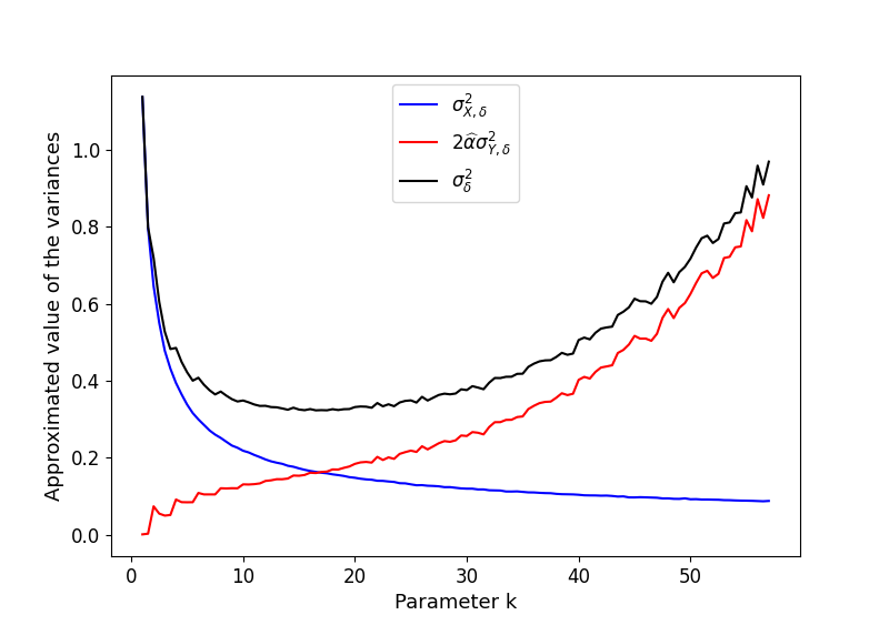
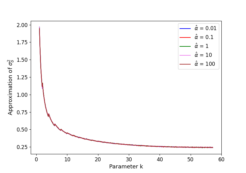
In the oscillating regime, we saw in Section 3.1 that we can significantly reduce the influence of $(Y_{t}^{\delta})_{t\geq 0}$ by choosing $\delta=\log(2)/\widehat{\alpha}$, see Figure 5. Thus, our conjecture is that even in the Gaussian regime, choosing $\delta=\log(2)/\widehat{\alpha}$ would allow us to have injectivity of $\sigma_{\delta}^{2}(.,\widehat{\alpha})$, because the impact of $\sigma_{Y,\delta}^{2}(.,\widehat{\alpha})$ will be significantly reduced. To check this hypothesis, we plot in Figure 7 the evolution of $\sigma_{\delta}^{2}(k,\widehat{\alpha})$ versus the parameter $k$ for several values of $\widehat{\alpha}$. If the curves that we obtained are injective, then our conjecture is valid. We see in Figure 7 that this is the case.

(a) $\sigma_{\delta}^{2}(k,\widehat{\alpha})$ (black), $\sigma_{X,\delta}^{2}(k,\widehat{\alpha})$ (blue) and $2\widehat{\alpha}\sigma_{Y,\delta}^{2}(k,\widehat{\alpha})$ (red) versus $k$, for $\widehat{\alpha}=1$.

(b) $\sigma_{\delta}^{2}(k,\widehat{\alpha})$ versus $k$ for $\widehat{\alpha}\in[0.01,0.1,1,10,100]$. The figure on the right shows that $\sigma_{\delta}^{2}(k,\widehat{\alpha})$ seems to be independent of the value of $\widehat{\alpha}$.

Figure 7. $\sigma_{\delta}^{2}(k,\widehat{\alpha})$ versus $k$ for $\delta=\log(2)/\widehat{\alpha}$, for different values of $\widehat{\alpha}$. To approximate $\sigma_{\delta}^{2}$ (and $\sigma_{X,\delta}^{2}$ and $\sigma_{Y,\delta}^{2}$ that compose it), we use $\overline{\sigma}_{\delta}^{2}$. The grid of parameters used to do the approximation is $\mathbb{G}_{1/10}$.

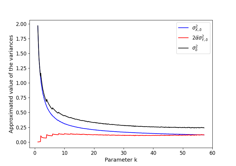
Then, for our inference in the Gaussian regime, we are going to use

$$\delta_{2}=\underset{i\Delta,\,i\in\llbracket 0,I\rrbracket}{\text{argmin}}\left|\Delta i-\log(2)/\widehat{\alpha}\right|.$$

When $\delta_{2}$ is sufficiently closed to $\log(2)/\widehat{\alpha}$, as we have observed in Figure 7(b) that $\sigma(k,\widehat{\alpha})$ seems independent of $\widehat{\alpha}$, we use $\overline{\sigma}_{\delta}^{2}(k,1)$ to approximate $\sigma(k,\widehat{\alpha})$. This allows us to save a lot of time for the computation of our “approximator” (that can take several days if we use a large mesh size), without compromising the quality of the results.

3.2.2. Quality of the estimation

Now that we know which time step we take, we study the quality of the estimation. We denote in this paragraph $(k_{1},\theta_{1})=(35,1)$, $(k_{2},\theta_{2})=(25.4,2)$, $(k_{3},\theta_{3})=(14.5,3.4)$, and $(k_{4},\theta_{4})=(44,1.5)$. As for all $l\in\llbracket 1,4\rrbracket$ we have $k_{l}<k_{c}$, these parameters are such that we are in the Gaussian regime, see Figure 1. For all $l\in\llbracket 1,5\rrbracket$, we have simulated $n_{\text{data}}=2000$ Bellman-Harris dynamics with lifetimes distributed according to $\Gamma(k_{l},\theta_{l})$, up to $8000$ cells. Then, for all $l\in\llbracket 1,5\rrbracket$, we create a dataset $(N_{l\Delta}^{(j)}:l\leq I,j\in\llbracket 1,n_{\text{data}}\rrbracket)$, where $I\in\mathbb{N}^{*}$, and denoting $\alpha_{l}=(2^{1/k_{l}}-1)/\theta_{l}$, $\Delta=\frac{\log(2)}{8\alpha_{l}}$.

We use the pipeline explained at the beginning of Section 3 to retrieve $(k_{i},\theta_{i})$ for all $i\in\llbracket 1,5\rrbracket$, see Figure 9. Then, we obtain an estimation of the mean and coefficient of variation of the distribution using the relation $(\mu,\frac{\sigma}{\mu})=(k\theta,1/\sqrt{k})$. For this inference, we use $\overline{\sigma}_{\delta}^{2}(k,1)$ to approximate $\sigma_{\delta}^{2}(k,\widehat{\alpha})$, see end of Section 3.2.1. The latter has been computed using a grid of parameters $\mathbb{G}_{1/20}$. The results of the estimation are given in Table 1. The scores that are the more relevant to consider are those for the estimation of $(\mu,\frac{\sigma}{\mu})$. We see that they are very good.

$(k,\theta)$ theoric	$(35,1)$	$(25.4,2)$	$(14.5,3.4)$	$(44,1.5)$
$(k,\theta)$ Param. infered	$(36.83,0.9504)$	$(25.42,1.999)$	$(14.57,3.384)$	$(41.71,1.582)$
$(k,\theta)$ Relative error	$(5.237\%,4.960\%)$	$(0.08081\%,0.04331\%)$	$(0.4893\%,0.4850\%)$	$(5.208\%,5.436\%)$
$(\mu,\frac{\sigma}{\mu})$ theoric	$(35,0.1690)$	$(50.8,0.1984)$	$(49.3,0.2626)$	$(66,0.1508)$
$(\mu,\frac{\sigma}{\mu})$ infered	$(35.00,0.1648)$	$(50.82,0.1983)$	$(49.30,0.2620)$	$(65.96,0.1548)$
$(\mu,\frac{\sigma}{\mu})$ Relative error	$(0.01732\%,2.520\%)$	$(0.03746)\%,0.4038\%)$	$(0.001927\%,0.2438\%)$	$(0.05514\%,2.710\%)$

.

Table 1. Results of the estimation in the Gaussian regime. The results are given with $4$ significant digits.

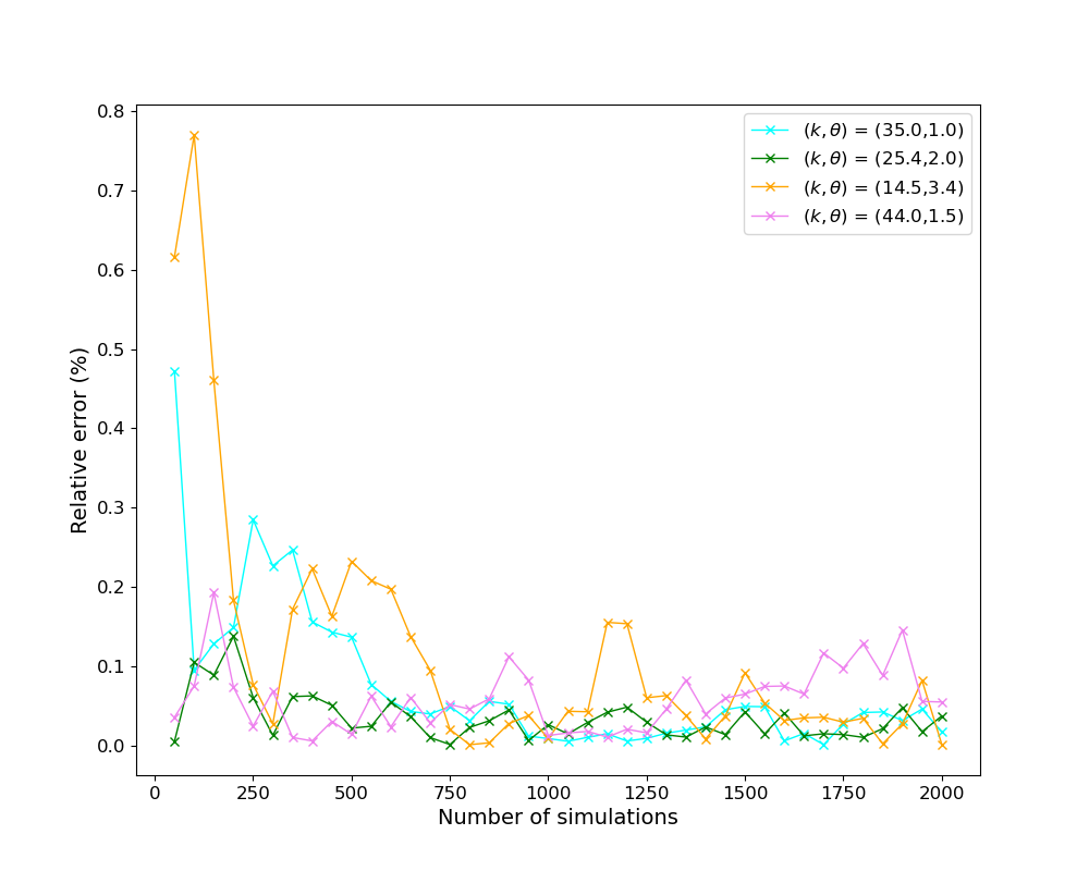
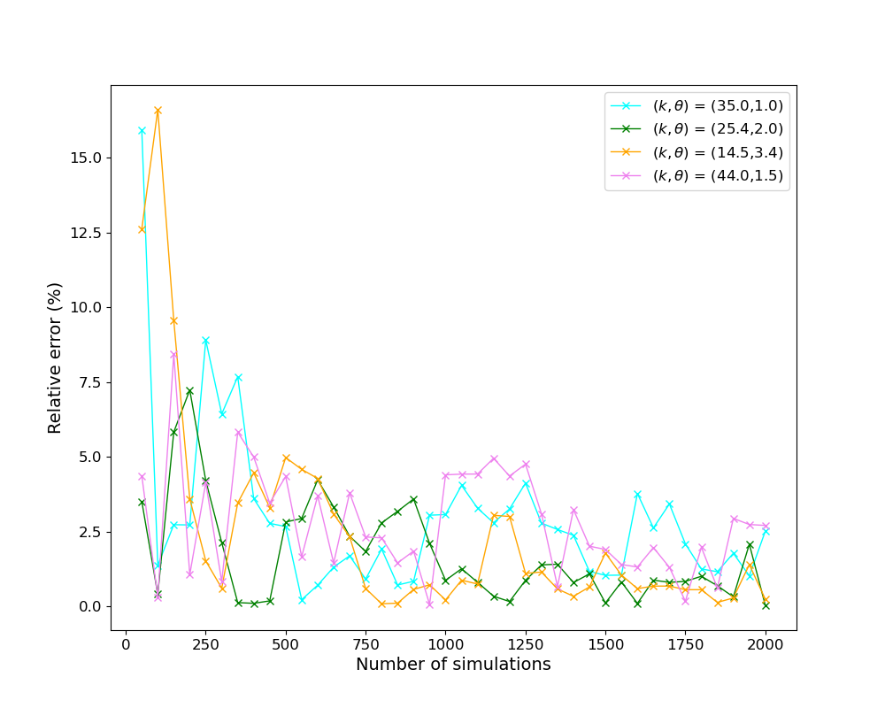
To do this estimation, we used $2000$ simulations. For applications on real data, we rarely have so many simulations. Let us check that the estimation still works even if we use fewer simulations. We use the pipeline to estimate $(\mu,\frac{\sigma}{\mu})$ for $n_{\text{data}}\in\left\{50l\,|\,l\in\llbracket 1,40\rrbracket\right\}$, and then we plot the relative error of the estimation versus $n_{\text{data}}$ in Figure 8. We see that with a small number of simulations, even if the score the relative error has increased, scores are still correct considering the fact that we do not have a lot of simulations. Indeed, for the estimation of $\mu$, even with a small number of simulations, all the relative errors are below $1\%$ as we see in Figure 8(a). For the estimation of $\sigma/\mu$, that corresponds to Figure 8(b), quickly we are under $10\%$ of relative error. Thus, the inference is satisfying for this regime.

(a) For $\mu$.

(b) For $\sigma/\mu$.

Figure 8. Relative error of the estimation versus the number of simulations for the inference in the Gaussian regime.

(a) Number of individuals along time.

(b) Number of individuals along time, at the log-scale. The mean of the coefficients of determination of the linear regressions done to obtain $\widehat{\alpha}$ is $R_{\text{mean}}^{2}=0.9998$.

(c) Fluctuations observed on simulations.

(d) Variance of fluctuations, at the log-scale. The coefficient of determination of the linear regression done to obtain $2\widehat{\lambda}$ is $R^{2}=0.9996$.

(e) Histogram of the fluctuations at the last observation time.

Figure 9. Illustration of the different steps for the inference with 2000 simulations, for parameters $(k_{1},\theta_{1})=(35,1)$.

3.3. Inference in the oscillating regime

Let us now consider the oscillating regime. By Figure 1, we know that we are in this regime when $k>k_{c}$. Thus, we study examples where this condition is satisfied. We run $n_{\text{data}}=2000$ simulations of Bellman-Harris processes with lifetimes distributed according to $\Gamma(k_{l},\theta_{l})$, with $l\in\llbracket 1,4\rrbracket$ and $(k_{1},\theta_{1})=(70,1)$, $(k_{2},\theta_{2})=(125,2)$, $(k_{3},\theta_{3})=(200.5,1)$, $(k_{4},\theta_{4})=(385.5,4)$. Then, we create a dataset from these simulations. The simulations and the creation of the dataset are done in the same way as in the Gaussian regime, see Section 3.2.2.

We use the pipeline described at the beginning of this section to recover the lifetime parameters and then the mean and coefficient of variation of the distribution, see Figure 11. The scores are displayed in Table 2. We see that the estimation of $(\mu,\frac{\sigma}{\mu})$ is very good, except in the case where $(k_{4},\theta_{4})=(385.5,2.5)$ for which the score is not as satisfying for $\frac{\sigma}{\mu}$. The reason is that when $k$ is very high, the amplitude of the oscillations is very large. Then, the linear regression done to obtain $\widehat{\lambda}$ is less reliable, as illustrated in Figure 12(d). For our motivation, cases with such low variability in cells lifetime are unrealistic, so this is not a significant issue.

Theoretical value of $(k,\theta)$	$(70,1)$	$(125,2)$	$(200.5,3)$	$(385.5,2.5)$
$(k,\theta)$ Param. inferred	$(77.78,0.9017)$	$(131.2,1.911)$	$(206.4,2.931)$	$(519.8,1.871)$
$(k,\theta)$ Relative error	$(11.11\%,9.835\%)$	$(4.947\%,4.444\%)$	$(2.940\%,2.315\%)$	$(34.83\%,25.15\%)$
Theoretical values of $(\mu,\frac{\sigma}{\mu})$	$(70,0.1195)$	$(250,0.08944)$	$(601.5,0.7062)$	$(963.8,0.05093)$
$(\mu,\frac{\sigma}{\mu})$ inferred	$(70.13,0.1134)$	$(250.7,0.08731)$	$(604.8,0.06961)$	$(972.7,0.04386)$
$(\mu,\frac{\sigma}{\mu})$ Relative error	$(0.1803\%,5.130\%)$	$(0.2833\%,2.385\%)$	$(0.5562\%,1.438\%)$	$(0.9251\%,13.88\%)$

Table 2. Results of the estimation in the oscillating regime. The results are given with $4$ significant digits.

To see the effect of the number of simulations, we plot the evolution of the relative error for $n_{\text{data}}\in\left\{50l\,|\,l\in\llbracket 1,40\rrbracket\right\}$ in Figure 10. Again, the results are good except for $(k_{4},\theta)=(385.5,2.5)$. The number of simulations seems to have a little influence on the relative error. Thus, the inference procedure seems very reliable for cases that motivate our study, and less precise for unrealistic cases with oscillations of large amplitude.

(a) For $\mu$.

(b) For $\sigma/\mu$.

Figure 10. Relative error of the estimation versus the number of simulations for the inference in the oscillating regime.

Estimation of the second eigenvalue based on the amplitude or on the frequency of the oscillations rather than a linear regression could improve the results in cases with large oscillations. As this is less relevant than a linear regression for the cases that motivate our study, we have not developed this type of estimation for the moment.

(a) Number of individuals along time.

(b) Number of individuals along time, at the log-scale. The mean of the coefficients of determination of the linear regressions done to obtain $\widehat{\alpha}$ is $R_{\text{mean}}^{2}=0.9995$.

(c) Fluctuations observed on simulations.

(d) Variance of fluctuations, at the log-scale. The coefficient of determination of the linear regression done to obtain $\widehat{\lambda}$ is $R^{2}=0.9926$.

Figure 11. Illustration of the different steps for the inference with 2000 simulations, for parameters $(k_{1},\theta_{1})=(70,1)$.

(a) Mean number of cells versus time, $(k_{1},\theta_{1})=(70,1)$. The mean of the coefficients of determination of the linear regressions done to obtain $\widehat{\alpha}$ is $R_{\text{mean}}^{2}=0.9995$.

(b) Mean number of cells versus time, $(k_{4},\theta_{4})=(385.5,2.5)$. The mean of the coefficients of determination of the linear regressions done to obtain $\widehat{\alpha}$ is $R_{\text{mean}}^{2}=0.9920$.

(c) Variance fluctuations versus time, $(k_{1},\theta_{1})=(70,1)$. The coefficient of determination of the linear regression done to obtain $\widehat{\lambda}$ is $R^{2}=0.9926$.

(d) Variance fluctuations versus time, $(k_{4},\theta_{4})=(385.5,2.5)$. The coefficient of determination of the linear regression done to obtain $\widehat{\lambda}$ is $R^{2}=0.8613$.

Figure 12. Comparison at the log-scale of the mean number of cells and variance of fluctuations, with exponential curves whose coefficients are respectively $\widehat{\alpha}$ and $2\widehat{\lambda}$, for $(k_{1},\theta_{1})=(70,1)$ and $(k_{4},\theta_{4})=(385.5,2.5)$. Mean and variance are computed using empirical estimators, with $2000$ simulations.

4. Estimation of parameters from data

Our original motivation for this work is the characterization of the variability of time division using monitoring of population sizes. Let us apply our work to two data counting dividing cells. All the quantities given below are given with $3$ significant numbers.

4.1. First data set

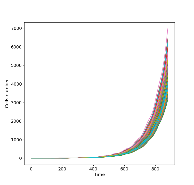
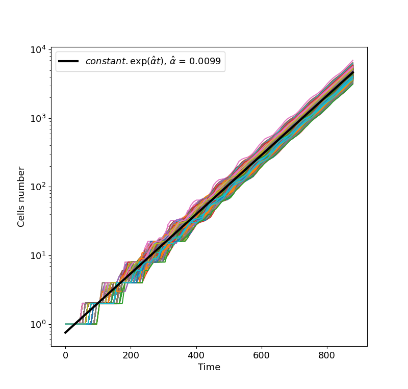
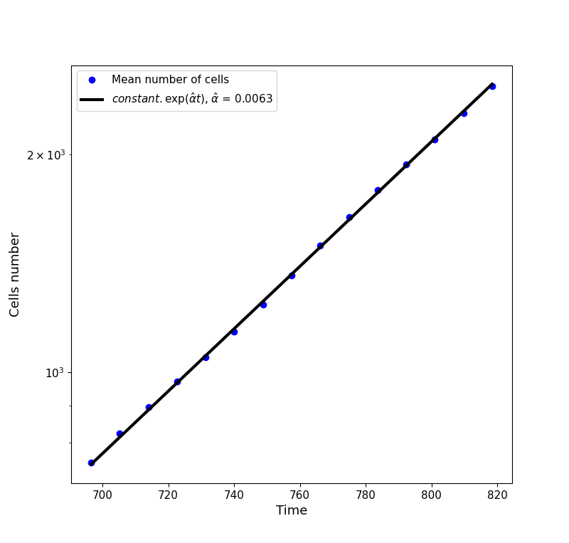
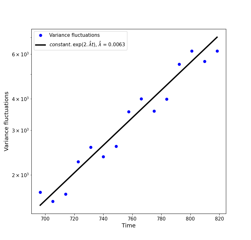
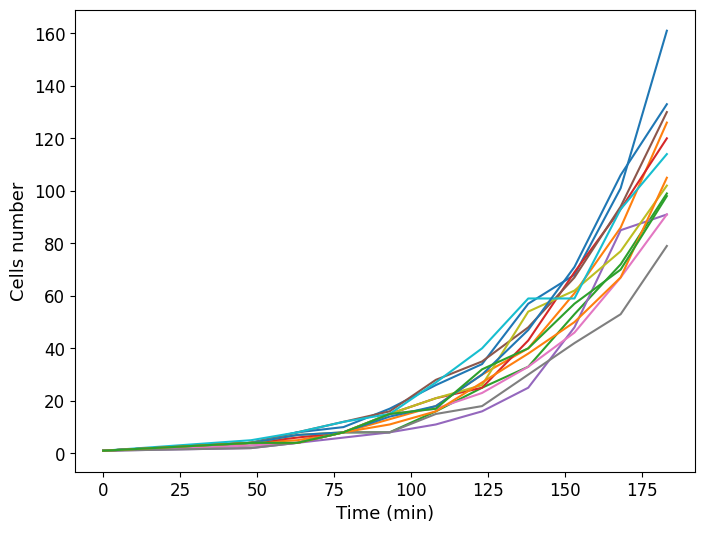
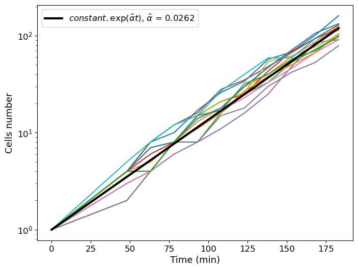
The first dataset we use comes from  [13]. It contains $13$ realizations of the growth of E. Coli bacteria, obtained with videomicroscopy, where the exact number of cells is counted in each frame. Measurements start after $48$ minutes, and are done every $15$ minutes, see Figure 13(a). Since the cells are grown in a very large recipient, we assume that they do not compete for resources, which is why they remain in exponential phase until the end of the measurements.

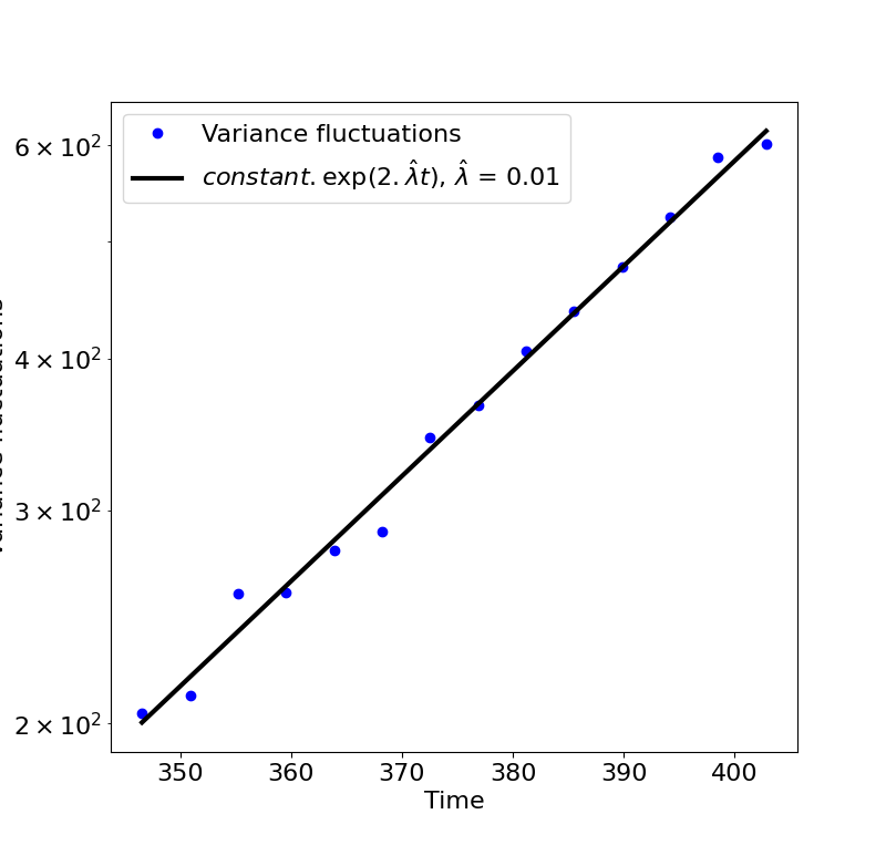
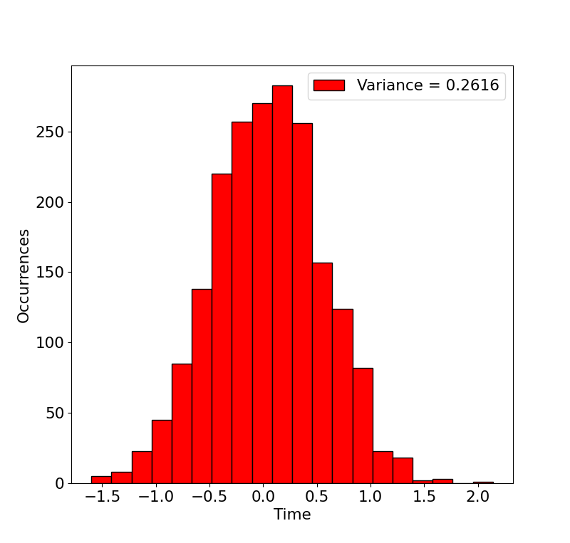
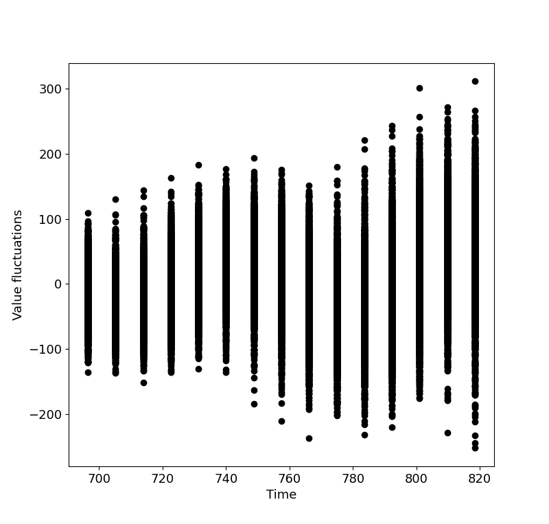
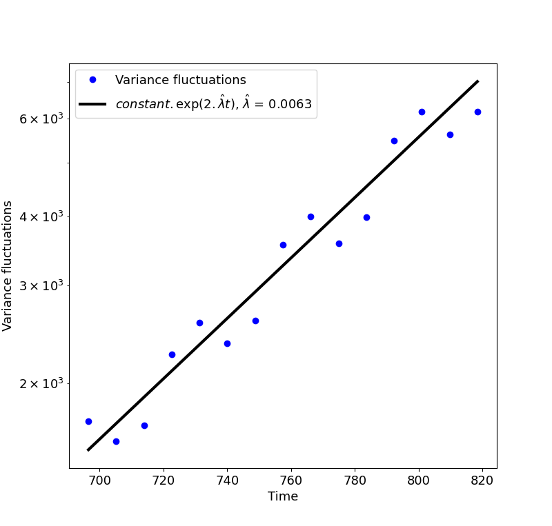
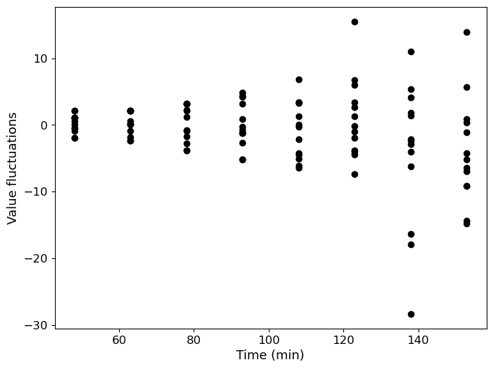
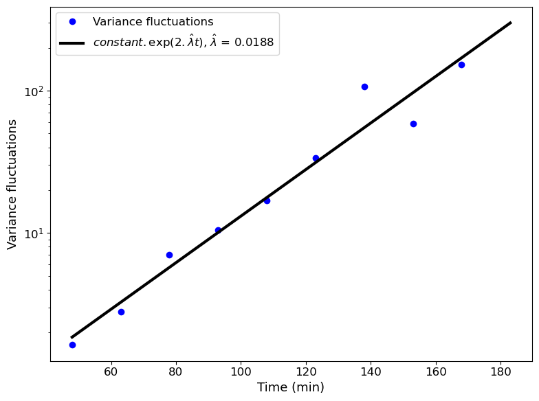
We suppose that the lifetime of these bacteria is distributed according to a Gamma distribution. Our aim is to estimate the mean and the coefficient of variation of bacteria lifetime with our method. First, we estimate the Malthusian coefficient and determine in which regime we are. The estimation of $\alpha$ gives us $\widehat{\alpha}_{1}=0.0262\text{ minutes}^{-1}$, see Figure 13(b). As we have $\log(2)/(2.\widehat{\alpha}_{1})=13.3\text{ minutes}$ and that $\Delta=15\text{ minutes}$, we use the time step $\delta_{1}=15\text{ minutes}$ to identify the regime. The result of the estimation of $\lambda$ is $\widehat{\lambda}_{1}~{}=~{}0.0188\text{ minutes}^{-1}$, see Figure 13(d). Then, we have the oscillating regime because

$$\frac{\left|2\widehat{\lambda}_{1}-\widehat{\alpha}_{1}\right|}{\widehat{\alpha}_{1}}=44.1\%>10\%.$$

We now estimate lifetime parameters. We use the estimator for the oscillating regime. Here are the parameters we obtain

$$(\widehat{k}_{1},\widehat{\theta}_{1}) =\underset{\begin{subarray}{c}(k,\theta)\in[1,+\infty[\times\mathbb{R}_{+}^{*}\\ (2^{1/k}-1)/\theta=\widehat{\alpha}_{1}\end{subarray}}{\text{argmin}}\left|(2^{1/k}\cos\left(2\pi/k\right)-1)/\theta-\widehat{\lambda}_{1}\right|=\left(102,0.260\text{ minutes}\right).$$

The latter corresponds to the following mean and coefficient of variation

$$\left(\widehat{\mu}_{1},\frac{\widehat{\sigma}_{1}}{\widehat{\mu}_{1}}\right)=\left(\widehat{k}_{1}\widehat{\theta}_{1},\frac{1}{\sqrt{\widehat{k}_{1}}}\right)=\left(26.6\text{ minutes},9.893\%\right).$$

Although the coefficient of variation is a little low, the values estimated seem fairly credible. Thus, the inference seems to have worked.

(a) Cells number at each time of measurement.

(b) Cells number at each time of measurement at the log-scale. The mean of the coefficients of determination of the linear regressions done to obtain $\widehat{\alpha}_{1}$ is $R_{\text{mean}}^{2}=0.986$.

(c) Fluctuations $R_{t,\delta_{1}}$ at each time of measurement.

(d) Variance of the fluctuations at each time of measurement, at the log-scale. The coefficient of determination of the linear regression done to obtain $\widehat{\lambda}_{1}$ is $R^{2}=0.960$.

Figure 13. Illustration of the different steps done to estimate the parameters of cells lifetime for the dataset coming from [13].

4.2. Second data set

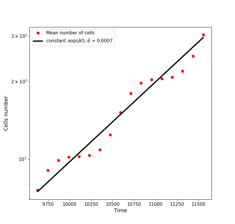
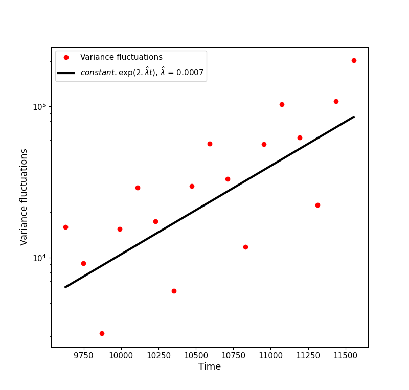
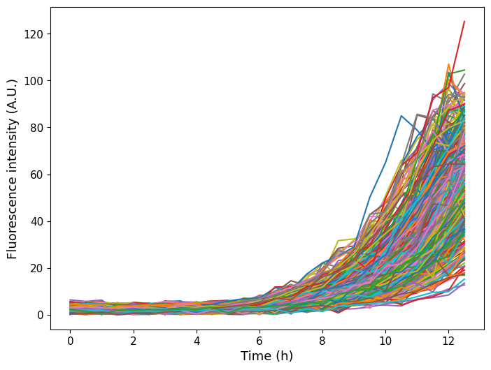
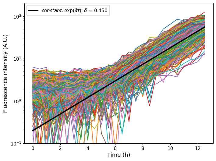
The second dataset we use comes from experiments conducted by the authors of the paper. Such data set is the original motivation for our study, see in particular [1, 9]. It contains $496$ realizations of the growth of bacteria E.Coli, obtained by encapsulating the original sets within anchored microfluidic droplets, see Figure 14(a). The drops are then placed on the stage of a motorized microscope and scanned at regular time intervals. Image analysis is then used to obtain the number of cells per droplet, as explained in  [24]. Here, the cells are grown in so-called MOPS minimal media, which explains their slow growth compared with typical cells growing in rich LB culture media [24]. The measurements are done every $30$ minutes, then $\Delta=0.5$ hours, and the number of bacteria is represented by an “intensity of fluorescence” in this dataset. It has been shown that there is a coefficient of proportionality between the intensity of fluorescence and the number of cells [9], although the value of this coefficient has not yet been found.

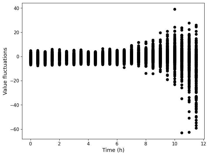
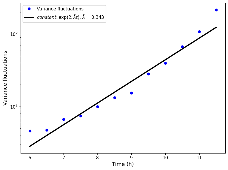
As for the first set, we want to obtain the mean and the coefficient of variation of the times between division of the bacteria thanks to our method. As we have a coefficient of proportionality between the number of cells and the intensity of fluorescence, eigenvalues remain the same in both setting. Thus, if we detect the oscillating regime, the inference is possible. The first thing we do is to estimate the Malthusian coefficient, and identify in which regime we are. We obtain thanks to linear regression that $\widehat{\alpha}_{2}=0.450\text{ hours}^{-1}$, see Figure 14(b). As $\log(2)/(2\widehat{\alpha}_{2})=0.770\text{ hours}$ and that $\Delta=0.5$ hours, we use $\delta_{1}=1$ hour to determine the regime. It is not a problem that $\delta_{1}$ is not close to $\log(2)/(2\widehat{\alpha}_{2})$. The more important is to avoid to be too close to $\log(2)/\widehat{\alpha}_{2}$, see Section 3.1.2, which is the case here. Our estimation of the second eigenvalue is $\widehat{\lambda}_{2}=0.343\text{ hours}^{-1}$, see Figure 14(d). We detect again the oscillating regime, because the relative error between $2\widehat{\lambda}_{2}$ and $\alpha$ is $52.4\%$, which is strictly greater than $10\%$. Then, using the formula we have used for the previous dataset yields

$$(\widehat{k}_{2},\widehat{\theta}_{2})=(120.1,\,0.0129\text{ hours}),$$

which corresponds to the following mean and coefficient of variation

$$\left(\widehat{\mu}_{2},\frac{\widehat{\sigma}_{2}}{\widehat{\mu}_{2}}\right)=\left(\widehat{k}_{2}\widehat{\theta}_{2},\frac{1}{\sqrt{\widehat{k}_{2}}}\right)=\left(1.55\text{ hours},9.12\%\right).$$

The value of $\mu_{2}$ obtained in this case is much higher than the one for the first dataset, in agreement with the slower growth rate observed in Figure 14. This is due to the different nature of the cell culture media. The estimated coefficient of variation appears to be fitting and relevant in this context. One can also see that we obtain a coefficient of variation similar to the one obtained in the previous dataset. Consequently, our estimation of variability also seems to work for this dataset.

(a) Cells number at each time of measurement.

(b) Cells number at each time of measurement, at the log-scale. The mean of the coefficients of determination of the linear regressions done to obtain $\widehat{\alpha}_{2}$ is $R_{\text{mean}}^{2}=0.926$.

(c) Fluctuations $R_{t,\delta_{1}}$ at each time of measurement.

(d) Variance of the fluctuations at each time of measurement, at the log-scale. The coefficient of determination of the linear regression done to obtain $\widehat{\lambda}_{2}$ is $R^{2}=0.954$.

Figure 14. Illustration of the different steps done to estimate the parameters of cells lifetime for the dataset coming from our experiments.

5. Discussion

In this work, we show how to obtain the parameters of the law of the lifespan of individuals using the total population sizes at given times. Our point of view is to exploit the distribution of fluctuations from one observation time to the next one. We model the population by a Bellman-Harris process and it does not include heredity. This provides a natural and simple statistical framework with independent and identically distribution lifespan. Despite this simplicity, the estimation of parameters of this distribution is subtle. Indeed, two regimes exist for the asymptotic fluctuations of the process. Determining in which regime we fall yields a first difficulty. It is worth noting that the critical value between the two regimes correspond to a coefficient variation of around $10\%$. This is realistic for biological problems and for instance for microfluidic data which motivates this work. This motivates a precise mathematical analysis. We propose a procedure to determine the regime of fluctuations and tune the length of the time between observations. This procedure has been confronted to simulations and real data. For simulations, our results show that the estimation we propose gives an efficient approach. The comparison with biological data also argues for its relevance. Indeed, applying our inference method on two different datasets returns mean and coefficient of variation that are consistent with our biological knowledge.

In many biological contexts (cell growth and cancer emergence, epidemics, invasive species…), obtaining the mean individual behavior is rather direct from the growth rate of the population size. Our study shows that determining the individual variability or stochasticity from measures at the population level is difficult. It puts in light that the choice of the times of observation is crucial. It also pledges for high sampling rate, and measures at the individual levels rather than at the population level. This would require us to generate lots of data using high magnification experiments. In contrast, by using the current techniques, we are able to measure the parameters of the division rates with a relatively low sampling time.

This work can be seen as first step for inverse problem and can pave the way for the investigation of more sophisticated and realistic models. In particular, one may focus on other distribution for the lifespan, even if it is less explicit than the Gamma law. For instance, the distribution of time for cell division is sometimes best described by the $a_{0}$-shifted gamma distribution, see [27] and references therein. A more challenging issue would be to take into account heredity. In particular, lots of attention has been paid to the effect of the size and of the variation of size from the previous division (size and adder model). This yields interesting perspectives. In particular, in this direction, robustness study and sensitivity analysis would be relevant. In our pursuit of capturing the variability in lifespan, we may also consider the initial individual differences through a mixed model.

At a more technical level, we expect to complement the results of Section 3 by more quantitative bounds on the estimation of parameters. In particular, the fact that we first estimate $\alpha$ and then use the value obtained for the estimation of the remaining parameter of the lifespan has been tested and validated by simulations but could be more formally investigated. Besides, we have used a threshold at $10\%$ for the detection of the Gaussian and oscillating regime from the data, based on empirical explorations. More generally, a sensitivity analysis would be interesting to complement this study and help for potential applications. It will also be valuable to obtain theoretical assurances on the property we have infered on $\sigma_{\delta}^{2}$ when $\delta=\ln(2)/\alpha$, as the injectivity of this function in the variable $k$, or the fact that it does not depend on $\alpha$.

6. Appendix and complements

6.1. Approximation of $h^{(\delta)}$

Function $h^{(\delta)}$ can not be approximated with Monte-Carlo simulations because the error of the empirical estimator of $h^{(\delta)}$ grows like $e^{\alpha t/2}$ when $t$ increases, in view of Theorem 1. In particular, if we denote $\widehat{h}^{(\delta)}$ the estimator obtained with Monte-Carlo simulations, the function

$$x\mapsto\text{Var}\left((\mathbb{E}_{x}\left[N_{\delta}\right]-e^{\alpha\delta})1_{[0,\zeta[}(x)+2\widehat{h}^{(\delta)}(x-\zeta)1_{[\zeta,+\infty[}(x)\right)e^{-\alpha\,x}$$

is not integrable. Thus, to approximate $h^{(\delta)}$, we proceed differently. We use the fact that the function $t\mapsto\mathbb{E}[N_{t}]$ can be approximated by the following

(37) $$\overline{\mathbb{E}[N_{t}]}=\frac{1}{2k}\sum_{l=-\left\lceil\frac{k}{2}\right\rceil+1}^{\left\lfloor\frac{k}{2}\right\rfloor}\frac{2^{\frac{1}{k}}\exp\left(\frac{2\pi\,l}{k}i\right)}{2^{\frac{1}{k}}\exp\left(\frac{2\pi\,l}{k}i\right)-1}\exp\left(\frac{2^{\frac{1}{k}}\exp\left(\frac{2\pi\,l}{k}i\right)-1}{\theta}t\right),$$

and approximate $h^{(\delta)}$ with $t\mapsto\overline{\mathbb{E}[N_{t+\delta}]}-e^{\alpha\delta}\overline{\mathbb{E}[N_{t}]}$.

In this section, we explain why we can approximate $t\mapsto\mathbb{E}[N_{t}]$ by the expression given in (37). When $k\in\mathbb{N}^{*}$, we show that the approximation is perfect. When $k\notin\mathbb{N}^{*}$, we obtain theoretical guarantees for large values of $t$.

6.1.1. Approximation when $k\in\mathbb{N}^{*}$

For all $t\geq 0$, we denote $m(t)=\mathbb{E}[N_{t}]$ and $\overline{G}(t)=1-G(t)$. Using the integral equation, we have

(38) $$m(t)=\overline{G}(t)+2\int_{0}^{t}m(t-s)g(s)ds=\overline{G}(t)+2\int_{0}^{t}m(s)g(t-s)ds.$$

Thus, taking the Laplace transform of $m$, we obtain that for all $p\in\mathbb{C}$ such that $Re(p)>\alpha$

$$\mathcal{L}m(p)=\mathcal{L}\overline{G}(p)+2\mathcal{L}g(p)\mathcal{L}m(p),$$

implying that

(39) $$\mathcal{L}m(p)=\frac{\mathcal{L}\overline{G}(p)}{1-2\mathcal{L}g(p)}.$$

We already know the explicit value of $\mathcal{L}g(p)$ by (19). In addition, with usual computations linked to the Laplace transform [18], we know that $\mathcal{L}\overline{G}(p)=\frac{\overline{G}(0)-\mathcal{L}g(p)}{p}=\frac{1-\mathcal{L}g(p)}{p}$. Combining these, and do a partial fraction decomposition, we obtain for all $p\in\mathbb{C}$ such that $Re(p)>\alpha$

$$\mathcal{L}m(p) =\frac{1}{p}\frac{(1+p\theta)^{k}-1}{(1+p\theta)^{k}-2}=\frac{1}{2k}\sum_{l=-\left\lceil\frac{k}{2}\right\rceil+1}^{\left\lfloor\frac{k}{2}\right\rfloor}\frac{2^{\frac{1}{k}}\exp\left(\frac{2\pi\,l}{k}i\right)}{2^{\frac{1}{k}}\exp\left(\frac{2\pi\,l}{k}i\right)-1}\frac{1}{p-\frac{2^{\frac{1}{k}}\exp\left(\frac{2\pi\,l}{k}i\right)-1}{\theta}}.$$

Now, with an analytic continuation and the fact that we know that for any $b\in\mathbb{C}$ the inverse Laplace transform of $p\mapsto 1/(p-b)$ is $t\mapsto e^{bt}$, we obtain that for all $t\geq 0$

$$m(t)=\frac{1}{2k}\sum_{l=-\left\lceil\frac{k}{2}\right\rceil+1}^{\left\lfloor\frac{k}{2}\right\rfloor}\frac{2^{\frac{1}{k}}\exp\left(\frac{2\pi\,l}{k}i\right)}{2^{\frac{1}{k}}\exp\left(\frac{2\pi\,l}{k}i\right)-1}\exp\left(\frac{2^{\frac{1}{k}}\exp\left(\frac{2\pi\,l}{k}i\right)-1}{\theta}t\right)=\overline{\mathbb{E}[N_{t}]}.$$

Thus, the formula given in (37) is the exact formula of the mean of the Bellman-Harris process when $k\in\mathbb{N}^{*}$.

6.1.2. Approximation when $k\notin\mathbb{N}^{*}$

When $k\notin\mathbb{N}^{*}$ (and $k\geq 1$), we can not do the partial fraction decomposition as done in the previous case. Nevertheless, (39) is still true. Thus, if we denote $f(t)=m(t)-1$, we have

$$\mathcal{L}f(p)=\frac{\mathcal{L}\overline{G}(p)}{1-2\mathcal{L}g(p)}-\frac{1}{p}=\frac{1}{p}\frac{1}{(1+p\theta)^{k}-2}.$$

The latter decreases to $0$ at a speed $Im(p)^{-(k+1)}$ when $Re(p)$ is constant and $Im(p)\rightarrow\pm\infty$. In particular, as $k\geq 1$, it is integrable along vertical lines. Moreover, as $g$ and $\overline{G}$ are continuous, in view of (38) and a domination, $m$ and then $f$ are continuous, so have local bounded variations. Then, we can use the Mellin’s inverse formula [31, Theorem $3.3$] to obtain that for all $\eta>\alpha$, $t\geq 0$,

(40) $$m(t) =1+\frac{1}{2i\pi}\int_{\eta-i\infty}^{\eta+i\infty}e^{pt}\mathcal{L}f(p)dp$$

$$=1+\frac{1}{2i\pi}\int_{\eta-i\infty}^{\eta+i\infty}e^{pt}\frac{1}{p}\frac{1}{(1+p\theta)^{k}-2}dp.$$

If we denote $F(p,t)=e^{pt}\frac{1}{p}\frac{1}{(1+p\theta)^{k}-2}$, and $\rho_{m}=\max\left(Re(\rho)\,|\,Re(\rho)>-1/\theta,\mathcal{L}(g)(\rho)=1/2\right)$, using the residue theorem, one can also obtain that for all $\vartheta\in\left(-1/\theta,\min(\rho_{m},0)\right)$,

$$\frac{1}{2i\pi}\int_{\eta-i\infty}^{\eta+i\infty}F(p,t)dp =\text{Res}_{p=0}\left(p\mapsto F(p,t)\right)+\sum_{\begin{subarray}{c}\rho\in\mathbb{C}\\ \mathcal{L}(g)(\rho)=1/2\\ Re(\rho)>-1/\theta\end{subarray}}\text{Res}_{p=\rho}\left(p\mapsto F(p,t)\right)$$

$$+\int_{\eta-i\infty}^{\vartheta-i\infty}F(p,t)dp+\int_{\vartheta-i\infty}^{\vartheta+i\infty}F(p,t)dp+\int_{\vartheta+i\infty}^{\eta+i\infty}F(p,t)dp,$$

which is equal, if we keep the position of each term, to

(41) $$\frac{1}{2i\pi}\int_{\eta-i\infty}^{\eta+i\infty}F(p,t)dp =-1+\frac{1}{2k}\sum_{\begin{subarray}{c}\rho\in\mathbb{C}\\ \mathcal{L}(g)(\rho)=1/2\\ Re(\rho)>-1/\theta\end{subarray}}\frac{2^{\frac{1}{k}}\exp\left(\frac{2\pi\,l}{k}i\right)}{2^{\frac{1}{k}}\exp\left(\frac{2\pi\,l}{k}i\right)-1}\exp\left(\frac{2^{\frac{1}{k}}\exp\left(\frac{2\pi\,l}{k}i\right)-1}{\theta}t\right)$$

$$+0+\int_{\vartheta-i\infty}^{\vartheta+i\infty}F(p,t)dp+0.$$

Plugging (41) in (40), we finally have that

(42) $$m(t) =\frac{1}{2k}\sum_{\begin{subarray}{c}\rho\in\mathbb{C}\\ \mathcal{L}(g)(\rho)=1/2\\ Re(\rho)>-1/\theta\end{subarray}}\frac{2^{\frac{1}{k}}\exp\left(\frac{2\pi\,l}{k}i\right)}{2^{\frac{1}{k}}\exp\left(\frac{2\pi\,l}{k}i\right)-1}\exp\left(\frac{2^{\frac{1}{k}}\exp\left(\frac{2\pi\,l}{k}i\right)-1}{\theta}t\right)+O(e^{\vartheta t})$$

$$=\overline{\mathbb{E}[N_{t}]}+O(e^{\vartheta t}).$$

Equation (42) gives a theoretical guarantee that $\overline{\mathbb{E}[N_{t}]}$ approximate $m(t)$ for large values of $t$. As $m(t)$ and $\overline{\mathbb{E}[N_{t}]}$ grow like an exponential, and as their difference vanishes exponentially, the “large values of $t$” come quickly. Moreover, as there are in (37) the eigenvalues that compose $t\mapsto m(t)$ (values such that $\mathcal{L}g=1/2$) with negative real part, we claim that the rest $O(e^{\vartheta t})$ has a well-approximated part. Indeed, taking an other contour to apply the residue theorem can be done to show that these terms partially compose the rest (nevertheless, there is still a part of the order of $e^{-\frac{t}{\theta}}$, so taking an other contour does not change the upper-bound we have for the rest). Thus, our approximation of $t\mapsto m(t)$ by $t\mapsto\mathbb{E}[N_{t}]$ seems reliable.

As we see in Figure 3, the value we use to approximate $h^{(\delta)}$ allows to obtain a very good numerical approximation of $\sigma_{\delta}^{2}$. This observation, that we have in practice, seems to support the fact that the approximation we use is relevant.

6.2. Variance of $N_{t}$ for Gamma law and sensitivity

In view of [7, $p.152-153$], there exists $n_{1}>0$, $n_{2}>0$ such that

$$\mathbb{E}[N_{t}]\underset{t\longrightarrow+\infty}{\sim}n_{1}e^{\alpha t},\text{ and }\text{Var}(N_{t})\underset{t\longrightarrow+\infty}{\sim}n_{2}e^{2\alpha t},$$

and such that

$$\frac{n_{2}}{(n_{1})^{2}}=\frac{4\mathcal{L}(g)(2\alpha)-1}{1-2\mathcal{L}(g)(2\alpha)}.$$

Using the expression of $\mathcal{L}(g)$ given in (19) to develop this ratio, and then using the fact that $k=\left(\mu/\sigma\right)^{2}$, we obtain (2), where for all $x\geq 0$

$$q(x)=\frac{4\left(2^{x^{2}+1}-1\right)^{-\frac{1}{x^{2}}}-1}{1-2\left(2^{x^{2}+1}-1\right)^{-\frac{1}{x^{2}}}}.$$

Let $\alpha=1$. We show now that $\phi(\sigma/\mu)=\sigma_{\delta}^{2}\left(1/(\sigma/\mu)^{2},\alpha\right)$, with $\delta=\log(2)/\alpha$, is more sensible to the variation of $\sigma/\mu$ than the quantity $q(\sigma/\mu)$ for $\sigma/\mu\leq 0.65$. In Figure 15(a), we first plot $\phi(\sigma/\mu,\alpha)$ versus $\sigma/\mu$, using the approximator $\overline{\sigma}_{\delta}^{2}$ of $\sigma_{\delta}^{2}$. We observe that the curve is almost linear, with a slope of $1.321$ (this is obviously not the case, but we will use this approximation). We have compared this value with the derivative of $q$ in Figure 15(b), and we see that the slope is always larger than the derivative of $q$ for $\sigma/\mu\in[1/(57.2)^{1/2},0.65]\simeq[0.1322,0.65]$.

(a) $\phi(\sigma/\mu)$ versus $\sigma/\mu$ for $\sigma/\mu\in[1/(57.2)^{1/2},1/2^{1/2}]$.

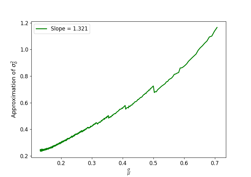
The coefficient of determination of the linear regression of $\phi$ versus the coefficient of variation is $R^{2}=0.9832$.

(b) $q^{\prime}(\sigma/\mu)$ versus $\sigma/\mu$ for $\sigma/\mu\in[1/(57.2)^{1/2},0.65]$ (red). Comparison with the slope of $\phi(\sigma/\mu,\theta)$ (blue).

Figure 15. Illustration that $\phi(\sigma/\mu)$ is more sensible to the variation of $\sigma/\mu$ than $q(\sigma/\mu)$. $\sigma_{\delta}^{2}$ has been approximated by $\overline{\sigma}_{\delta}^{2}$ to plot these curves, using the grid of parameters $\mathbb{G}_{1/20}$ to compute it

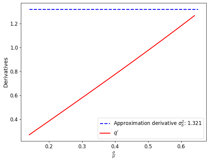
Then, in view of the mean value inequality and using the approximation that $\phi$ is linear, we can conclude that for all $(a,b)\in[1/(57.2)^{1/2},0.65]$

$$\frac{|q(b)-q(a)|}{|b-a|}\leq\max_{x\in[a,b]}|q^{\prime}(x)|\leq 1.321\approx\frac{\left|\phi(b,\theta)-\phi(a,\theta)\right|}{|b-a|}.$$

Thus, $\phi(\sigma/\mu)^{2}(\sigma/\mu,\theta)$ is more sensible to the variation of $\sigma/\mu$ that the quantity $q(\sigma/\mu)$, when $\sigma/\mu\in[1/(57.2)^{1/2},0.65]$. This interval contains most of the biologically-relevant coefficient of variations in the Gaussian regime. Then, $\sigma_{\delta}^{2}$ seems more relevant to use than $q$ to obtain information on the variability of division times.

For coefficient of variations greater than $0.65$, the coefficient of variation seems too large compared to what is biologically true. If we ignore this, even if $q$ is more sensible, there is still difficulties to use $q$ in practice, due to the fact that there are a lot of source of randomness coming from the early stages of the experiment [27]. Our method of estimation do not have these problems, that’s why we think it is still more relevant to use it rather than $q$.

6.3. Extension of the asymptotic fluctuations to Bellman-Harris processes

Theorem 1 can be extended to Bellman-Harris processes that satisfy the following assumptions:

1. The reproduction law has a finite third and fourth moment, and the probability to give no offspring is $0$. In addition, the first moment of this law, that we denote $m$, is strictly greater than $1$.

2. Lifetime distribution is given by a density $g$, that is bounded continuous on $\mathbb{R}_{+}$, and continuously differentiable on $(0,+\infty)$. In addition, $g^{\prime}$ is bounded on intervals of the form $[\eta,+\infty)$, where $\eta>0$.

3. The following holds

   $$\sup_{s\geq 0}\left|\frac{g(s)}{1-G(s)}\right|<+\infty.$$

4. For all $\delta>0$, there exists $C>0$, $l>-2$ such that (we denote $G$ the cumulative distribution linked to $g$) for all $a>0$

   $$\sup_{x\in[0,\delta]}\left|\frac{\frac{\partial\,g(a+x)}{\partial\,a}(a,x)}{1-G(a)}\right|\leq C\left(a^{l}1_{a<1}+1\right).$$

5. For all $\lambda\in\mathbb{C}$ such that $\mathcal{L}(g)(\lambda)=1/m$, $\left(\mathcal{L}\right)^{\prime}(g)(\lambda)\neq 0$.

Indeed, conditions on the moments of the reproduction law, given by Assumption $(A)$, imply Lemma 1 $(i)$ . Adding the boundedness and the continuity of $g$, given by $(B)$, allow to obtain Lemma 1 $ii)-iii)$. Then, we get Proposition 1 from Lemma 1.

Now, using the fact that $g^{\prime}$ is bounded on intervals of the form $[\eta,+\infty)$, where $\eta>0$, and the inequalities presented in $(C)$ and $(D)$, we obtain an analog to Lemma 2 $i)$: $h_{1}$ is continuously differentiable, and there exists $C_{h_{1}}>0$ such that $h_{1}(a)\leq C_{h_{1}}(a^{l}+1)$. Now, as done for the gamma distribution, we obtain an equivalent to Lemma 2 $ii)$ from $i)$: there exists $C_{h_{2}}>0$ such that $Vh_{2}(a)\leq C_{h_{2}}1_{\{a\geq 0\}}(1+\min(a,1)^{l+1}+a)$. The proof of Lemma 2 $iii)$ does not change. We finally apply [21, Theorem $2.8$], for which me need to have $m>1$, to obtain Propositions 2 and 3, and conclude the proof by similar steps as those presented in the proof of Theorem 1.

We require to have a probability to give no offspring to $0$, to be sure that we have $W>0$ a.s., and then that we can divide $R_{t,\delta}$ by $W$. This assumption can be relaxed by considering events where the population survives. Assumption $(E)$ can also be relaxed, but the analytic expression presented in Theorem 1 $ii)-iii)$ must be adapted, adding polynomial terms. We refer to [21] for that.

6.4. The exponential case

The case of exponential lifetimes seems not relevant for modeling many biological phenomenons such as the time between two divisions. In that case, the memory less property allows to simplify the analysis. The behavior of the fluctuations

$$R_{t}^{\delta}=N_{t+\delta}-e^{\delta\alpha}\,N_{t},$$

is simply obtained by a classical central limit theorem. Indeed,

$$R_{t}^{\delta}=\sum_{i=1}^{N_{t}}\left(N_{t,\delta}^{i}-e^{\delta\alpha}\right),$$

and $(N_{t,\delta}^{i}-e^{\delta\alpha}:1\leq i\leq N_{t})$ are i.i.d. variables independent of $N_{t}$. Then, if we denote $\nu>0$ the parameter of the exponential law, as for all $i\in 1\leq i\leq N_{t}$, $\text{Var}\left(N_{t,\delta}^{i}\right)=e^{2\nu\delta}-e^{\nu\delta}$, we have

$$R_{t}^{\delta}\overset{\mathcal{L}}{\underset{t\longrightarrow+\infty}{\Longrightarrow}}\mathcal{N}\left(0,e^{2\nu\delta}-e^{\nu\delta}\right).$$

In particular, there is one single regime, the Gaussian one, with a simple interpretation of the limiting variance.

As an exponential law is a gamma law with parameter $k=1$, this result can also be obtained with Theorem 1.

Acknowledgement. We warmly thank Marc Hoffmann for stimulating discussions on this topic and this work. We also thank Antoine Barizien for his preliminary investigations. This work was partially funded by the Chair “Modélisation Mathématique et Biodiversité” of VEOLIA-Ecole Polytechnique-MNHN-F.X., by the European Union (ERC, SINGER, 101054787), and by the Fondation Mathématique Jacques Hadamard. Views and opinions expressed are however those of the author(s) only and do not necessarily reflect those of the European Union or the European Research Council. Neither the European Union nor the granting authority can be held responsible for them.

Authors’ contributions. Jules Olayé has conducted this work for the mathematical part, the simulations and the estimations from data. Vincent Bansaye and Charles Baroud have supervised this work. Antoine Barizien and Vincent Bansaye have made the first investigations. Jules Olayé and Hala Bouzidi have realized a project during their Master 2, which have given the first theoretical and numerical results of this paper. Andrey Aristov and Salomé Gutiérrez Ramos have realized the microfuidics experiments. Jules Olayé and Vincent Bansaye have written the paper based on all these contributions.

References

- [1] Gabriel Amselem, Cyprien Guermonprez, Benoît Drogue, Sébastien Michelin and Charles N. Baroud “Universal microfluidic platform for bioassays in anchored droplets” In Lab on a Chip 16.21, 2016, pp. 4200–4211 DOI: 10.1039/C6LC00968A
- [2] Søren Asmussen “Applied Probability and Queues” 51, Stochastic Modelling and Applied Probability, 2003 DOI: 10.1007/b97236
- [3] Krishna B. Athreya “Limit theorems for multitype continuous time Markov branching processes. I. The case of an eigenvector linear functional” In Zeitschrift für Wahrscheinlichkeitstheorie und Verwandte Gebiete 12.4, 1969, pp. 320–332 DOI: 10.1007/BF00538753
- [4] Krishna B. Athreya “Limit theorems for multitype continuous time Markov branching processes. II. The case of an arbitrary linear functional” In Zeitschrift für Wahrscheinlichkeitstheorie und Verwandte Gebiete 13.3, 1969, pp. 204–214 DOI: 10.1007/BF00539201
- [5] Krishna B. Athreya and Nayile Kaplan “Convergence of the Age Distribution in the One-Dimensional Supercritical Age-Dependent Branching Process.” In The Annals of Probability 4.1, 1976, pp. 38–50 DOI: 10.1214/aop/1176996179
- [6] Krishna B. Athreya and Soumendra N. Lahiri “Measure Theory and Probability Theory”, Springer Texts in Statistics, 2006 DOI: 10.1007/978-0-387-35434-7
- [7] Krishna B. Athreya and Peter E. Ney “Branching Processes” 196, Grundlehren der mathematischen Wissenschaften, 1972 DOI: 10.1007/978-3-642-65371-1
- [8] Frank Ball and Peter Donnelly “Strong approximations for epidemic models” In Stochastic Processes and their Applications 55.1, 1995, pp. 1–21 DOI: 10.1016/0304-4149(94)00034-Q
- [9] Antoine Barizien “Studying the variability of bacterial growth in microfluidicdroplets”, 2019 URL: https://theses.hal.science/tel-02168120
- [10] Antoine Barizien, Mani sai Suryateja Jammalamadaka, Gabriel Amselem and Charles N. Baroud “Growing from a few cells: combined effects of initial stochasticity and cell-to-cell variability” In Journal of The Royal Society Interface 16.153, 2019 DOI: 10.1098/rsif.2018.0935
- [11] Frédérique Billy, Jean Clairambault, Olivier Fercoq, Stéphane Gaubert, Thomas Lepoutre, Thomas Ouillon and Shoko Saito “Synchronisation and control of proliferation in cycling cell population models with age structure” In Mathematics and Computers in Simulation 96, 2014, pp. 66–94 DOI: 10.1016/j.matcom.2012.03.005
- [12] Tom Britton and Etienne Pardoux “Stochastic Epidemic Models with Inference” 2255, Lecture Notes in Mathematics, 2019 DOI: 10.1007/978-3-030-30900-8
- [13] Jessica Coates, Bo Ryoung Park, Dai Le, Emrah Şimşek, Waqas Chaudhry and Minsu Kim “Antibiotic-induced population fluctuations and stochastic clearance of bacteria” In eLife 7, 2018 DOI: 10.7554/eLife.32976
- [14] Stephen Cooper “Bacterial Growth and Division”, 1991 DOI: 10.1016/B978-0-08-091747-4.50008-4
- [15] Alexander M.. Cox, Simon C. Harris, Emma L. Horton and Andreas E. Kyprianou “Multi-species Neutron Transport Equation” In Journal of Statistical Physics 176.2, 2019, pp. 425–455 DOI: 10.1007/s10955-019-02307-2
- [16] Kenny S. Crump and Charles J. Mode “A general age-dependent branching process. I” In Journal of Mathematical Analysis and Applications 24.3, 1968, pp. 494–508 DOI: https://10.1016/0022-247X(68)90005-X
- [17] Richard Durrett “Branching Process Models of Cancer” 1.1, Mathematical Biosciences Institute Lecture Series, 2015 DOI: 10.1007/978-3-319-16065-8
- [18] Gerald B. Folland “Fourier Analysis and Its Applications”, Wadsworth and Brooks/Cole Mathematics Series, 2009
- [19] Patsy Haccou, Peter Jagers and Vladimir A. Vatutin “Branching Processes: Variation, Growth, and Extinction of Populations” 5, Cambridge Studies in Adaptive Dynamics, 2005 DOI: 10.1017/CBO9780511629136
- [20] Theodore E. Harris “The Theory of Branching Processes” 1, Grundlehren der mathematischen Wissenschaften, 1963 URL: https://link.springer.com/book/9783642518683
- [21] Alexander Iksanov, Konrad Kolesko and Matthias Meiners “Asymptotic fluctuations in supercritical Crump-Mode-Jagers processes” Preprint v2, 2023 URL: http://arxiv.org/abs/2109.00867
- [22] Hye-Jeong Kang “Central limit theorems for Bellman-Harris processes” In Journal of the Korean Mathematical Society 36.5, 1999, pp. 923–943 URL: https://jkms.kms.or.kr/journal/view.html?spage=923&volume=36&number=5
- [23] Marek Kimmel and David E. Axelrod “Branching Processes in Biology” 19, Interdisciplinary Applied Mathematics, 2015 DOI: 10.1007/978-1-4939-1559-0
- [24] Lena Le Quellec, Andrey Aristov, Salomé Gutiérrez Ramos, Gabriel Amselem, Julia Bos, Zeynep Baharoglu, Didier Mazel and Charles N. Baroud “Measuring single-cell susceptibility to antibiotics within monoclonal bacterial populations” Preprint, 2023 DOI: 10.1101/2023.03.08.531654
- [25] A.. Lloyd “Realistic distributions of infectious periods in epidemic models: changing patterns of persistence and dynamics” In Theoretical Population Biology 60.1, 2001, pp. 59–71 DOI: 10.1006/tpbi.2001.1525
- [26] Sylvie Meleard and Vincent Bansaye “Stochastic Models for Structured Populations”, Mathematical Biosciences Institute Lecture Series 1, 2015 DOI: 10.1007/978-3-319-21711-6
- [27] Evgeny B. Stukalin, Ivie Aifuwa, Jin Seob Kim, Denis Wirtz and Sean X. Sun “Age-dependent stochastic models for understanding population fluctuations in continuously cultured cells” In Journal of The Royal Society Interface 10.85, 2013 DOI: 10.1098/rsif.2013.0325
- [28] Sattar Taheri-Araghi, Serena Bradde, John T. Sauls, Norbert S. Hill, Petra Anne Levin, Johan Paulsson, Massimo Vergassola and Suckjoon Jun “Cell-Size Control and Homeostasis in Bacteria” In Current Biology 25.3, 2015, pp. 385–391 DOI: 10.1016/j.cub.2014.12.009
- [29] Vladimir A. Vatutin “Polling Systems and Multitype Branching Processes in Random Environment with Final Product” In Theory of Probability & Its Applications 55.4, 2011, pp. 631–660 DOI: 10.1137/S0040585X97985078
- [30] Ping Wang, Lydia Robert, James Pelletier, Wei Lien Dang, Francois Taddei, Andrew Wright and Suckjoon Jun “Robust growth of Escherichia coli” In Current biology 20.12, 2010, pp. 1099–1103 DOI: 10.1016/j.cub.2010.04.045
- [31] David V. Widder “The Laplace Transform”, Princeton Mathematical Series, 1946 URL: https://press.princeton.edu/books/hardcover/9780691653693/laplace-transform-pms-6