Conditions for growth and extinction in matrix models with environmental stochasticity

Abstract

In this kind of model, the main characteristic that determines population viability in the long term is the stochastic growth rate (SGR) denoted $\lambda_{S}$. When $\lambda_{S}$ is larger than one, the population grows exponentially with probability one and when it is smaller than one, the population goes extinct with probability one. However, even in very simple situations it is not possible to calculate the SGR analytically. The literature offers some approximations for the case in which environmental variability is low, and there are also some lower and upper bounds, but there is no study of the practical situations in which they would be tight. Some new bounds for the SGR are built and the conditions under which each bound works best are analyzed. These bounds are used to give some necessary and some sufficient conditions for population explosion and extinction that are easy to check in practice. The general results are applied to several cases, amongst them a population structured as juveniles and adults living in an environment switching randomly between ”rich” and ”poor”.

keywords:matrix models, environmental stochasticity, stochastic growth rate, lower bound, upper bound, extinction.

1 Introduction

We consider matrix population models that incorporate environmental stochasticity, which refers to unpredictable temporal fluctuations in environmental conditions. A number of different environmental conditions are considered and their variation is characterized by a sequence of random variables corresponding to the different time steps of the discrete system (Tuljapurkar, 1990; Caswell, 2001). Each environment is characterized by its corresponding population projection matrix (PPM), i.e., the matrix of vital rates in that environment, e.g., time-specific annual PPMs gained from a time-series of data (Logofet, 2018; elsewhere in this Issue). It is well known that, given certain hypotheses on the pattern of temporal variation and on the set of PPMs, the total population size grows (or decays) exponentially with probability one, with a rate given by the so called stochastic growth rate $\lambda_{\mathrm{S}}$ (SGR), which is the stochastic analogue of the dominant eigenvalue for deterministic systems.

The SGR is the main feature of this kind of models due to its ecological implications, and it is widely used by ecologists as a measure of population fitness (Williams et al., 2015; Compagnoni et al., 2016; McDonald et al., 2016; Gremer and Venable, 2014). A SGR larger than one implies population explosion with probability one whereas a value lower than one implies that the population tends to extinction with probability one. It must be stressed that we are adopting Cohen’s definition for the SGR (Cohen, 1979) because it allows one to directly compare the stochastic rate of growth with its deterministic counterpart, although some authors (Tuljapurkar, 1990; Caswell, 2001) define the SGR as the logarithmic rate of growth, i.e., $\log\lambda_{\mathrm{S}}$.

The SGR is easy to obtain for scalar models, i.e., in the case of unstructured populations (Alonso and Sanz, 2009). However (letting aside some settings in which very specific conditions are met (Tuljapurkar, 1990; Alonso and Sanz, 2009)), it can not be derived analytically for structured populations. Indeed, even in relatively simple cases like stochastic Leslie models with two age classes, there are no closed-form expressions for the SGR.

As a result, in order to obtain the SGR, the main tools at the ecologist’s disposal are computer simulations(Williams et al., 2015; Gremer and Venable, 2014), certain perturbation techniques like Tuljapurkar’s approximation, $\lambda_{T},$ to the SGR (see (Tuljapurkar, 1990) for the derivation and (Davison et al., 2013) for an application) and, in certain systems with time scales, approximate aggregation techniques that allow one to transform the original system to a scalar one (Sanz and Bravo de la Parra, 2007; Alonso and Sanz, 2009; Sanz and Alonso, 2010).

Another strategy that offers valuable information is the derivation of upper and lower bounds for the SGR. In addition to the quantitative values of these bounds, ecologists can make use of them to extract qualitative information about the model in the following way: assume that one knows that

$$c\leq\log\lambda_{\mathrm{S}}\leq C,$$ (1)

(throughout this work, and for the sake of simplicity in the expressions involved, bounds for $\log\lambda_{\mathrm{S}},$ rather than for $\lambda_{\mathrm{S}}$ itself, will be considered. Obviously bounds for $\lambda_{\mathrm{S}}$ follow in the form $\exp(c)\leq\lambda_{\mathrm{S}}\leq\exp(C)$). Then, the population grows to infinity with probability one when $c>0$, whereas whenever $C<0$ the population goes extinct with probability one. Therefore, the bounds can be used to obtain sufficient (although not necessary) conditions for population growth or extinction.

In the mathematical literature, there are some bounds for the SGR that can be quite precise, but they must be obtained through complex algoritmic procedures, so that there are no closed-form expressions for them (see (Protasov and Jungers, 2013) and the references therein). In this work, however, we are interested in bounds that can be easily obtained and that, at least in two-stage models, can be obtained analytically. The literature on mathematical ecology presents a few bounds with those properties (Cohen, 1979; Caswell, 2001). One of them is $\mu$, the rate of growth of the mean population size, which is an upper bound. Several works have compared $\lambda_{\mathrm{S}}$ and $\mu$ (see (Tuljapurkar, 1990) and the references therein). However, there is hardly any study on the conditions under which the other bounds work well or a comparison between the different bounds. An exception was given by (Tuljapurkar and Orzack, 1980), who discussed a case in which one of the bounds is very loose and therefore of little practical interest. Neither are there studies that use the bounds to obtain analytical conditions for growth or extinction as suggested above.

The first purpose of this work is to find new upper and lower bounds for the SGR. Different approaches are followed and, as a consequence, four different upper and lower bounds will be obtained. One of the approaches is only valid in the context of stochastic Leslie models with two age classes, but the rest of the bounds are valid for general stage-classified models. Moreover, in the case of models with two stages, closed-form expressions for the bounds are provided.

Our second aim is to provide some properties of both the new and known bounds and, moreover, to give some ideas about the situations in which each one performs best. In addition, a comparison between the different bounds is carried out.

Finally, in order to illustrate their usefulness in a practical application, the bounds are used to obtain conditions that guarantee non-extinction in a Leslie model with two age classes and two possible environments.

The structure of the paper is as follows: Section 2 introduces the basic setting of matrix models with environmental stochasticity and the concept of SGR. The general setting is particularized in 2.1 to a stochastic Leslie model with two age classes that will be used throughout the paper to illustrate the different results we provide. Section 3 presents the different bounds already available in the literature and some of their properties. In Section 4, we make use of a perturbation approach to obtain a new result that is valid for any kind of stochastic matrix model. It allows one to compare the SGR of two stochastic systems that share the same pattern of environmental variability but have different PPMs. Then we make use of this general result in order to obtain three new bounds for the SGR.

Section 5 concentrates in the specific case of stochastic Leslie models with two age classes, and provides bounds that are built by making use of some properties of age structure.

An analysis and comparison of the different bounds is carried out in Section 6 in the context of the aforementioned stochastic Leslie model with young and adults and two environments. We also relate the bounds with Tuljapurkar’s second-order approximation $\lambda_{T}$ to the SGR (Tuljapurkar, 1982).

Section 7, towards which ecologists interested mainly in applications can focus their attention, illustrates one of the possible uses of the bounds to obtain analytical conditions for growth or extinction of populations in a setting in which a population is subjected to a rich and a poor environment. A discussion of results can be found in Section 8. The manuscript is completed with an Appendix that contains different proofs together with an important auxiliary result on stochastic matrix population models.

2 Matrix models with environmental stochasticity

We assume that the population lives in an ambient in which there are different environmental states, which we suppose indexed by $\eta\in\mathcal{I}$ where $\mathcal{I}$ is a set of indexes (examples are $\mathcal{I}=\left\{1,...,r\right\}$, $\mathcal{I}=\mathbb{Z}_{+}$ or $\mathcal{I}=\mathbb{R}_{+}$). The vital rates corresponding to environment $\eta\in\mathcal{I}$ are given by the nonnegative PPM $\boldsymbol{A}_{\eta}=\left[A_{\eta}^{ij}\right]_{1\leq i,j\leq n}\in\mathbb{R}_{+}^{n\times n}$ and $\mathcal{A}=\{\boldsymbol{A}_{\eta},\ \eta\in\mathcal{I}\}$ is the set of different PPMs.

Note that $\mathcal{I}$ can theoretically be infinite, numerable or denumerable, yet for the sake of simplicity we express all expectations considering the numerable case, i.e., in terms of (possible infinite) sums. In the denumerable case all expressions are still valid but the sums must be replaced with the corresponding integrals.

Environmental randomness is characterized by a homogeneous Markov chain $\tau_{t}$, $t=0,1,2,...$ defined on a certain probability space $(\Omega,\mathcal{F},p)$ (Billingsley, 2008) over the state space $\mathcal{I}$. For each realization $\omega\in\Omega$ of the process, the population is subjected to environmental conditions $\tau_{t+1}(\omega)$ between times $t$ and $t+1$.

Thus, the model reads

$$\boldsymbol{z}(t+1)=\boldsymbol{A}_{\tau_{t+1}}\boldsymbol{z}(t),$$ (2)

where for each $t=0,1,...$, $\boldsymbol{z}(t)=\left(z^{1}(t),...,z^{n}(t)\right)^{\text{T}}$ is a vector random variable in $\mathbb{R}^{n}$ which represents the population vector at time $t$. The total population is $\left\|\boldsymbol{z}(t)\right\|_{1}:=\left|z^{1}(t)\right|+\cdots+\left|z^{n}(t)\right|$ (the subscript at the norm notation will be further omitted). Throughout we assume that $\boldsymbol{z}_{0}$ is a fixed nonnegative nonzero vector.

Assume that $\tau_{t}$ has a unique stationary probability distribution given by $\boldsymbol{\pi}=\left[\pi_{\eta}\right]_{\eta\in I}$ towards which the $t$-step transition probabilities converge, i.e., $\pi_{\eta}:=\lim_{t\rightarrow\infty}p\left(\tau_{t}=\eta\mid\tau_{0}=\xi\right)$ for all $\eta,\xi\in\mathcal{I}$. It is well known (see A for a precise statement of the result) that if the set $\mathcal{A}$ is ergodic and an additional technical condition on the speed of convergence of these transition probabilities is met, then:

1. The joint process $\left(\tau_{t},\boldsymbol{z}(t)/\left\|\boldsymbol{z}(t)\right\|\right)$ is a Markov chain that converges to a certain stationary distribution $G$.

2. There exists the so called stochastic growth rate $\lambda_{\mathrm{S}}$ (SGR) of system (2), defined through

   $$\log\lambda_{\mathrm{S}}:=\underset{t\rightarrow\infty}{\lim}\log\left\|\boldsymbol{z}(t)\right\|/t,$$ (3)

   where the limit holds with probability one. Moreover, $\lambda_{\mathrm{S}}$ is finite and independent of the initial probabilities of the chain states and of the initial (non-zero) population vector $\boldsymbol{z}_{0}\geq\boldsymbol{0}$.

It follows from (3) that if $\log\lambda_{\mathrm{S}}>0,$ then the population grows exponentially to infinity with probability one, whereas it becomes extinct with probability one whenever $\log\lambda_{\mathrm{S}}<0$. We assume the conditions for the existence of the SGR to hold true throughout this work.

In the next sections several upper and lower bounds for the SGR will be obtained. Clearly, a desirable property of a SGR bound is that, when there is no environmental variation (i.e., in the deterministic case), it coincides with the dominant eigenvalue of the corresponding PPM. Specifically:

Property P. We say that a (lower or upper) bound $C$ for the SGR verifies property P when in the case $\boldsymbol{A}_{\eta}=\boldsymbol{A}$ for all$\ \eta\in\mathcal{I}$ it follows that $C=\rho(\boldsymbol{A}),$ where $\rho$ denotes the spectral radius.

It will be shown that some, but not all, of the bounds studied in this work verify property P.

2.1 A particular case: stochastic Leslie model with two age clases

As an illustration of the general setting above we turn our attention to the case of Leslie models with $n=2$ age classes, juveniles and adults. The model takes the form

$$\left(\begin{array}[c]{c}\boldsymbol{z}^{1}(t+1)\\ \boldsymbol{z}^{2}(t+1)\end{array}\right)=\boldsymbol{A}_{\tau_{t+1}}\left(\begin{array}[c]{c}\boldsymbol{z}^{1}(t)\\ \boldsymbol{z}^{2}(t)\end{array}\right),$$ (4)

where

$$\boldsymbol{A}_{\eta}:=\left(\begin{array}[c]{cc}f_{\eta}&F_{\eta}\\ s_{\eta}&0\end{array}\right),\ \eta\in\mathcal{I}.$$

This simple model will be used to illustrate the different results obtained.

In model (4), a necessary and sufficient condition for the set $\mathcal{A}$ of vital rates to be ergodic is that there exist positive constants $\alpha$ and $\beta$ such that for all $\eta\in\mathcal{I}$, $f_{\eta}$, $F_{\eta}$ and $s_{\eta}$ are bounded from above by $\beta$ and from below by $\alpha$. In that case, for any non-zero initial condition $\boldsymbol{z}(0)$ the population vector $\boldsymbol{z}(t)$ is positive for all $t\geq 2$.

The mean matrix with respect to the stationary environmental distribution $\boldsymbol{\pi}$ is

$$\boldsymbol{\bar{A}}:=\left(\begin{array}[c]{cc}\bar{f}&\bar{F}\\ \bar{s}&0\end{array}\right),$$ (5)

where

$$\bar{f}:=\sum_{\eta\in\mathcal{I}}\pi_{\eta}f_{\eta},\ \bar{F}:=\sum_{\eta\in\mathcal{I}}\pi_{\eta}F_{\eta},\ \bar{s}:=\sum_{\eta\in\mathcal{I}}\pi_{\eta}s_{\eta}.$$

3 Known bounds for the SGR

This section shows the bounds already known in the literature. Specifically, the rate of growth of the mean population size, Cohen’s bounds and the bounds through a max-min approach are considered. Later on, they will be compared with the new bounds proposed in this work.

Rate of growth of the mean population size. An important parameter in models of the kind (2) is the rate of growth, $\mu,$ of the mean population size, i.e.,

$$\log\mu:=\underset{t\rightarrow\infty}{\lim}\log\mathbb{E}\left\|\boldsymbol{z}(t)\right\|/t.$$ (6)

It is well known that, as an immediate consequence of Jensen’s inequality (Billingsley, 2008), one has

$$\lambda_{\mathrm{S}}\leq\mu,$$ (7)

and so $\mu$ is an upper bound for the SGR. Note that one can have apparently paradoxical situations in which $\log\mu>0$ and so the mean population size grows to infinity, whereas $\log\lambda_{\mathrm{S}}<0,$ and so the population goes extinct with probability one. This illustrates the sufficient yet unnecessary essence of condition $\log\mu<0$ for population extinction.

The literature shows (Cohen, 1979) that $\mu$ coincides with the dominant eigenvalue of a certain nonnegative matrix $\boldsymbol{D}$ that, in the general Markovian case, depends on matrices $\boldsymbol{A}_{\eta}$ and on the one-step transition probabilities of the chain $\tau_{t}$. If, for the sake of simplicity, we restrict our attention to the case in which $\tau_{t}$ is an independent and identically distributed (IID) process, $\boldsymbol{D}$ coincides with the mean environmental matrix, i.e.,

$$\boldsymbol{\bar{A}}:=\sum_{\eta\in\mathcal{I}}\pi_{\eta}\boldsymbol{A}_{\eta}.$$ (8)

It is easy to check that when there is no environmental variability, matrix $\boldsymbol{D}$ coincides with the deterministic matrix $\boldsymbol{A}$ and so $\mu$ verifies property P.

In the case of system (4) and IID temporal variation, one has

$$\log\mu=\log\rho(\mathbf{\bar{A}})=\log\frac{\bar{f}+\left(\bar{f}^{2}+4\bar{F}\bar{s}\right)^{1/2}}{2}.$$

When imposing the sufficient condition for extinction $\mu<1,$ the resulting analytical expression can be simplified by using the concept of net reproductive value in matrix models (Cushing and Yicang, 1994). Indeed if $R_{0}=\bar{f}+\bar{s}\bar{F}$ denotes the net reproductive value corresponding to matrix $\boldsymbol{\bar{A}}$, the condition $\mu<1$ is equivalent to $R_{0}<1$, i.e., $\bar{f}+\bar{s}\bar{F}<1$ which is, therefore, a sufficient condition for the extinction of the population.

Cohen’s bounds. For each $\eta\in\mathcal{I}$, define the column sums of $\boldsymbol{A}_{\eta}$

$$\varphi_{\eta}^{j}:=\overset{n}{\underset{i=1}{\sum}}A_{\eta}^{ij},\ j=1,...,n\text{, }\eta\in\mathcal{I},$$ (9)

and let $m_{\eta}$ and $M_{\eta}$ be their respective minimum and maximum, i.e.,

$$m_{\eta}=\underset{j=1,...,n}{\min}\varphi_{\eta}^{j},\ \ \ M_{\eta}=\underset{j=1,...,n}{\max}\varphi_{\eta}^{j},\ \eta\in\mathcal{I}.$$

Then (Cohen, 1979) one has $c_{I}\leq\log\lambda_{\mathrm{S}}\leq C_{I}$ where

$$c_{I}:=\underset{\eta\in\mathcal{I}}{\sum}\pi_{\eta}\log m_{\eta},\ \ C_{I}:=\underset{\eta\in\mathcal{I}}{\sum}\pi_{\eta}\log M_{\eta}.$$ (10)

In (Tuljapurkar and Orzack, 1980) certain numerical simulations are carried out that show that, at least in the cases covered in the study, bounds (10) do not work well. Bounds (10) are tight when for each $\eta\in\mathcal{I}$ all the columns of $A_{\eta}$ sum approximately to the same amount, and the contrary happens when the maximum and the minimum of the column sums are very different. Indeed, it is easy to check that they are exact if and only if $\boldsymbol{A}_{\eta}=\alpha_{\eta}\boldsymbol{P}$ for each $\eta\in\mathcal{I}$, where $\alpha_{\eta}\in\mathbb{R}$ and $\boldsymbol{P}$ is a column-stochastic matrix.

Another problem of bounds (10) is that they do not verify property P, i.e., they do not coincide with the SGR when there is no environmental variation.

In the case of system (4), one has

$$c_{I}:=\underset{\eta\in\mathcal{I}}{\sum}\pi_{\eta}\log\min\left\{f_{\eta}+s_{\eta},F_{\eta}\right\},\ C_{I}:=\underset{\eta\in\mathcal{I}}{\sum}\pi_{\eta}\log\max\left\{f_{\eta}+s_{\eta},F_{\eta}\right\}.$$ (11)

Bounds through a max-min approach. It is immediate to show that if $\boldsymbol{\tilde{A}},\boldsymbol{\hat{A}}\in\mathbb{R}^{n\times n}$ are non-negative matrices such that

$$0\leq\boldsymbol{\tilde{A}}\leq\boldsymbol{A}_{\eta}\leq\boldsymbol{\hat{A}},\ \eta\in\mathcal{I},$$

then $c_{\min}\leq\log\lambda_{\mathrm{S}}\leq C_{\max}$ where

$$c_{\min}:=\log\rho(\boldsymbol{\tilde{A}}),\ C_{\max}:=\log\rho(\boldsymbol{\hat{A}})$$ (12)

Clearly, these bounds are very easy to obtain and verify property P. A serious drawback is that they are independent of the equilibrium environmental distribution $\boldsymbol{\pi}$ and so they do not weight the relative contribution of the different environments. For instance, when there is only two environments and $\boldsymbol{A}_{1}<\boldsymbol{A}_{2}$, it is easy to see that $c_{\min}$ is very poor whenever $\pi_{1}$ is close to zero.

In the case of system (4), one has

$$\boldsymbol{\tilde{A}}=\left(\begin{array}[c]{cc}\underset{{}^{\eta\in\mathcal{I}}}{\min}f_{\eta}&\underset{{}^{\eta\in\mathcal{I}}}{\min}F_{\eta}\\ \underset{{}^{\eta\in\mathcal{I}}}{\min}s_{\eta}&0\end{array}\right),\ \boldsymbol{\hat{A}}=\left(\begin{array}[c]{cc}\underset{{}^{\eta\in\mathcal{I}}}{\max}f_{\eta}&\underset{{}^{\eta\in\mathcal{I}}}{\max}F_{\eta}\\ \underset{{}^{\eta\in\mathcal{I}}}{\max}s_{\eta}&0\end{array}\right).$$ (13)

4 A perturbation approach to obtaining bounds for the SGR

Let us first introduce a new result that relates the SGR of any two stochastic systems of the kind (2). Although more general in nature, this result will be particularized to certain situations to obtain bounds for the SGR.

Consider the following stochastic system:

$$\boldsymbol{z}^{\prime}(t+1)=\boldsymbol{B}_{\tau_{t+1}}\boldsymbol{z}^{\prime}(t),$$ (14)

where we assume that $\left\{\boldsymbol{B}_{\eta},\eta\in\mathcal{I}\right\}$ is an ergodic set of $n\times n$ non-negative matrices and, further, that their incidence matrices coincide with those of system (2), that is, for all $\eta\in\mathcal{I}$ one has $B_{\eta}^{ij}=0$ if and only if $A_{\eta}^{ij}=0$.

Under the above conditions there exists an SGR, that we denote $\lambda_{\mathrm{S}}^{\prime},$ for (14). Now we want to relate $\lambda_{S}$ and $\lambda_{\mathrm{S}}^{\prime}$. In order to do so, let us first define matrices $\boldsymbol{W}_{\eta}=\left[W_{\eta}^{ij}\right]_{1\leq i,j\leq n}$, $\eta\in\mathcal{I}$ through

$$W_{\eta}^{ij}:=\left\{\begin{tabular}[c]{c}$\frac{A_{\eta}^{ij}-B_{\eta}^{ij}}{B_{\eta}^{ij}}\text{ if }B_{\eta}^{ij}\neq 0$\\ $0\text{ if }B_{\eta}^{ij}=0$\end{tabular}\ \ .\right.$$ (15)

Note that $W_{\eta}^{ij}$ can be thought of as the relative amount of perturbation of $A_{\eta}^{ij}$ with respect to $B_{\eta}^{ij}$. Let us now set

$$W_{\eta}^{m}:=\min_{i,j=1,...,n}W_{\eta}^{ij},\ \ W_{\eta}^{M}:=\max_{i,j=1,...,n}W_{\eta}^{ij}.$$ (16)

Using the nonnegativity of $\boldsymbol{A}_{\eta}$ and $\boldsymbol{B}_{\eta}$ and the fact that the incidence matrix of $\boldsymbol{B}_{\eta}$ coincides with that of $\mathbf{A}_{\eta}$, we check immediately that

$$W_{\eta}^{M}\geq W_{\eta}^{m}>-1.$$ (17)

Then (see B) one has

$$\log\lambda_{\mathrm{S}}^{\prime}+\underset{\eta\in\mathcal{I}}{\sum}\pi_{\eta}\log\left(1+W_{\eta}^{m}\right)\leq\log\lambda_{S}\leq\log\lambda_{\mathrm{S}}^{\prime}+\underset{\eta\in\mathcal{I}}{\sum}\pi_{\eta}\log\left(1+W_{\eta}^{M}\right).$$ (18)

The previous result is more general, but in this work it is used in the case in which system (14) is deterministic, i.e., $\boldsymbol{B}_{\eta}=\boldsymbol{B}$ for all $\eta\in\mathcal{I}$ where $\boldsymbol{B}$ is a certain matrix, so that $\lambda_{\mathrm{S}}^{\prime}=\rho(\boldsymbol{B})$. Therefore in that case one can write $c_{\text{pert}}\leq\log\lambda_{S}\leq C_{\text{pert}}$ where

$$c_{\text{pert}}:=\log\rho(\boldsymbol{B})+\underset{\eta\in\mathcal{I}}{\sum}\pi_{\eta}\log\left(1+W_{\eta}^{m}\right),\ C_{\text{pert}}:=\log\rho(\boldsymbol{B})+\underset{\eta\in\mathcal{I}}{\sum}\pi_{\eta}\log\left(1+W_{\eta}^{M}\right).$$ (19)

Bounds $c_{\text{pert}}$ and $C_{\text{pert}}$ have been deduced through a perturbation approach and certainly work better when, for each $\eta\in\mathcal{I},$ matrix $\boldsymbol{A}_{\eta}$ is a perturbation of $\boldsymbol{B}$. However, the bounds are valid even when that is not the case. We stress that these bounds are valid in systems of general dimensionality, i.e., $n$ is arbitrary.

Note that when there is no stochasticity $W_{\eta}^{m}=W_{\eta}^{M}=0$ for all $\eta\in\mathcal{I},$ and so the bounds in (19) verify property P as desired.

Obviously different choices of matrix $\boldsymbol{B}$ will lead to different bounds. We propose three possibilities:

1. $\boldsymbol{B}$ equals the average environmental matrix. We take

$$\boldsymbol{B}=\boldsymbol{\bar{A}}:=\mathbb{E}_{\pi}(\boldsymbol{A}_{\tau_{t}})=\underset{\eta\in\mathcal{I}}{\sum}\pi_{\eta}\boldsymbol{A}_{\eta},$$

i.e., the average environmental matrix with the average taken with respect to the stationary distribution of $\tau_{t}$. We denote $c_{II}$ and $C_{II}$ the resulting bounds in (19) for this choice of $\boldsymbol{B}$.

In the case of system (4) we have

$$c_{II} =\log\frac{\bar{f}+\left(\bar{f}^{2}+4\bar{F}\bar{s}\right)^{1/2}}{2}+\underset{\eta\in\mathcal{I}}{\sum}\pi_{\eta}\log\min\left\{1,\frac{f_{\eta}}{\bar{f}},\frac{F_{\eta}}{\bar{F}},\frac{s_{\eta}}{\bar{f}}\right\},$$

$$C_{II} =\log\frac{\bar{f}+\left(\bar{f}^{2}+4\bar{F}\bar{s}\right)^{1/2}}{2}+\underset{\eta\in\mathcal{I}}{\sum}\pi_{\eta}\log\max\left\{1,\frac{f_{\eta}}{\bar{f}},\frac{F_{\eta}}{\bar{F}},\frac{s_{\eta}}{\bar{f}}\right\}.$$

Note that for system (4) and the IID setting, one has $C_{II}\geq\log\rho(\boldsymbol{\bar{A}})=\log\mu$ and therefore in this case $\log\mu$ is always better than $C_{II}$ as an upper bound for $\log\lambda_{\mathrm{S}}$.

2. $\boldsymbol{B}$ equals the “max-matrix”. We define $\boldsymbol{B}=\left[B^{ij}\right]_{1\leq i,j\leq n}$ through

$$B^{ij}=\underset{\eta\in\mathcal{I}}{\max}A_{\eta}^{ij},$$

and we denote $c_{III}$ and $C_{III}$ the resulting bounds in (19).

In this case $\boldsymbol{B}=\boldsymbol{\hat{A}}$ in (12) and $W_{\eta}^{M}\leq 0$ for all $\eta\in\mathcal{I}$. Therefore $C_{III}\leq\log\rho(\boldsymbol{\hat{A}})=C_{\max}$ and so $C_{III}$ is always a better upper bound than $C_{\max}$.

For system (4) one has $W_{\eta}^{M}=0$ for all $\eta\in\mathcal{I}$ and so

$$c_{III}=\log\frac{\max\nolimits_{\eta}f_{\eta}+\left(\left(\max\nolimits_{\eta}f_{\eta}\right)^{2}+4\left(\max\nolimits_{\eta}F_{\eta}\right)\left(\max\nolimits_{\eta}s_{\eta}\right)\right)^{1/2}}{2}+$$ (20)

$$+\underset{\eta\in\mathcal{I}}{\sum}\pi_{\eta}\log\left(1+\min\left\{\frac{f_{\eta}}{\max\nolimits_{\eta}f_{\eta}},\frac{F_{\eta}}{\max\nolimits_{\eta}F_{\eta}},\frac{s_{\eta}}{\max\nolimits_{\eta}s_{\eta}}\right\}\right),$$

$$C_{III}=C_{\max}=\log\frac{\max\nolimits_{\eta}f_{\eta}+\left(\left(\max\nolimits_{\eta}f_{\eta}\right)^{2}+4\left(\max\nolimits_{\eta}F_{\eta}\right)\left(\max\nolimits_{\eta}s_{\eta}\right)\right)^{1/2}}{2}.$$

3. $\boldsymbol{B}$ equals the “min-matrix”. We put

$$B^{ij}=\underset{\eta\in\mathcal{I}}{\min}A_{\eta}^{ij},$$

and the resulting bounds in (19) are denoted $c_{IV}$ and $C_{IV}$. Reasoning like in the previous case, one has $c_{IV}\geq\log\rho(\boldsymbol{\tilde{A}})=c_{\min}$ and therefore $c_{IV}$ is always a better lower bound than $c_{\min}$. In the case of system (4), one has analogous expressions for $c_{IV}$ and $C_{IV}$ to those of (20).

We emphasize that the bounds $C_{III}$ and $c_{IV}$ proposed in this work improve the existing bounds $C_{\max}$ and $c_{\min}$ respectively.

There is no rule of thumb for the best choice of matrix $B,$ even in very simple situations as when there are only two stages, only one vital rate varies and there are two environments which are equiprobable. Simulations show that, in general, the optimal choice of $B$ is somewhere inbetween the “min” and the “max” matrices, sometimes close to the former, some to the latter and some others to the average matrix.

5 Bounds in two-class Leslie models

The idea is to find bounds for the vector of age structure, i.e., the vector with the proportion of young and adults, that are valid for large times and that can be used later on to obtain bounds for the SGR. As a first step, we generalize some results from (Tuljapurkar, 1990) to obtain bounds for the vector of age structure when all three vital rates (fertility of the young, of the adults and survival) are stochastic. These bounds on age structure are then used to obtain a new bound for the SGR.

5.1 Bounds on age structure for two-class Leslie models

We are interested in finding bounds for age structure valid for large values of $t$, i.e., we want to find (deterministic) vectors $\boldsymbol{l}=\left(l^{1},...,l^{n}\right),\boldsymbol{u}=\left(u^{1},...,u^{n}\right)\in\mathbb{R}_{+}^{n},$ such that for large enough $t$ one can write

$$\boldsymbol{l}\leq\frac{\boldsymbol{z}(t)}{\left\|\boldsymbol{z}(t)\right\|}\leq\boldsymbol{u}$$ (21)

These bounds on age structure are relevant in this work since, as it is shown later on, they can be used to obtain new bounds for the SGR.

It is not possible to obtain bounds of the kind (21) for system (2) in the general case. In (Tuljapurkar, 1990) certain bounds are obtained in the particular case of Leslie models, although when there is an arbitrary number of age classes the bounds can not be obtained through closed expressions but must be found through an iterative process. Here we concentrate in the case of system (4) with $n=2$ age classes, for which closed form expressions can be found.

First we obtain bounds for the quotient $z^{2}(t)/z^{1}(t)$ in the form

$$\delta\leq\frac{z^{2}(t)}{z^{1}(t)}\leq\kappa.$$ (22)

Once this is accomplished, it is immediate to conclude that the vector of population structure can be bounded as follows

$$\left(\frac{\delta}{1+\kappa},\frac{1}{1+\kappa}\right)=:\boldsymbol{l}\leq\frac{\boldsymbol{z}(t)}{\left\|\boldsymbol{z}(t)\right\|}\leq\boldsymbol{u}:=\left(\frac{\kappa}{1+\delta},\frac{1}{1+\delta}\right).$$ (23)

In (Tuljapurkar, 1990) bounds of the kind (22) are obtained in the case in which only the survival of the young is stochastic. Here we show that, following a similar reasoning to that of (Tuljapurkar, 1990), the results can be extended to the case in which the three vital rates are stochastic. Specifically, let us define

$$\varepsilon_{M}:=\underset{\eta\in\mathcal{I}}{\max}\frac{F_{\eta}}{f_{\eta}},\ \varepsilon_{m}:=\underset{\eta\in\mathcal{I}}{\min}\frac{F_{\eta}}{f_{\eta}},\ \gamma_{M}:=\underset{\eta\in\mathcal{I}}{\max}\frac{s_{\eta}}{f_{\eta}},\ \gamma_{m}:=\underset{\eta\in\mathcal{I}}{\min}\frac{s_{\eta}}{f_{\eta}}.$$

Then it can be shown (see B for the proof) that equation (22) holds with

$$\delta =\frac{2\gamma_{m}}{1-\varepsilon_{m}\gamma_{m}+\varepsilon_{M}\gamma_{M}+\sqrt{1+(\varepsilon_{M}\gamma_{M}-\varepsilon_{m}\gamma_{m})^{2}+2(\varepsilon_{M}\gamma_{M}+\varepsilon_{m}\gamma_{m})}},$$ (24)

$$\kappa =\frac{2\gamma_{M}}{1-\varepsilon_{M}\gamma_{M}+\varepsilon_{m}\gamma_{m}+\sqrt{1+(\varepsilon_{m}\gamma_{m}-\varepsilon_{M}\gamma_{M})^{2}+2(\varepsilon_{m}\gamma_{m}-\varepsilon_{M}\gamma_{M})}}.$$

Note that, in the deterministic setting, i.e., $\boldsymbol{A}_{\eta}=\boldsymbol{A}$ for all $\eta\in\mathcal{I}$, bounds $\delta$ and $\kappa$ coincide with the quotient $v^{2}/v^{1}$ where $\boldsymbol{v}=(v^{1},v^{2})$ is a right eigenvector of matrix $\boldsymbol{A}$ associated to its dominant eigenvalue, and so bounds (23) are exact.

5.2 Bounds for the SGR using info on age structure

Consider system (2) and assume that (21) holds for certain known vectors $\boldsymbol{l}$ and $\boldsymbol{u}$. Then it follows (see B for the proof) that $c_{V}\leq\log\lambda_{\mathrm{S}}\leq C_{V}$ where

$$c_{V}:=\underset{\eta\in\mathcal{I}}{\sum}\pi_{\eta}\log\left(\overset{n}{\underset{j=1}{\sum}}l_{\eta}^{j}\varphi_{\eta}^{j}\right),\ C_{V}:=\underset{\eta\in\mathcal{I}}{\sum}\pi_{\eta}\log\left(\overset{n}{\underset{j=1}{\sum}}u^{j}\varphi_{\eta}^{j}\right),$$ (25)

and the $\varphi_{\eta}^{j}$ are given by (9).

Note that in the deterministic case one has $\boldsymbol{l}=\boldsymbol{u}$ and so bounds (25) are exact.

In principle these bounds can be used for any system of the kind (2), but as mentioned before, in practice bounds of the kind (21) are not at our disposal. In the particular case of model (4), by making use of (23) one obtains

$$c_{V}:=\underset{\eta\in\mathcal{I}}{\sum}\pi_{\eta}\log\left(\frac{f_{\eta}+s_{\eta}+F_{\eta}\delta}{1+\kappa}\right),\ C_{V}:=\underset{\eta\in\mathcal{I}}{\sum}\pi_{\eta}\log\left(\frac{f_{\eta}+s_{\eta}+F_{\eta}\kappa}{1+\delta}\right),$$

where $\delta$ and $\kappa$ are given by (24).

6 Analysis and comparison of the different bounds

In this section we carry out a comparison of the different bounds which have been previously introduced. Before we proceed, it should be noted that, excluding $\mu$, the rest of the bounds considered in this work depend on the environmental chain $\tau_{t}$ only through its equilibrium distribution $\boldsymbol{\pi}$ and are therefore independent of the serial correlation between different environments. On the other hand, we stress that previous studies (Tuljapurkar, 1982) show that the SGR depends strongly on the stationary distribution $\boldsymbol{\pi}$ but rather weakly on the serial correlation between environments. Taking these two facts into consideration, in order to carry out the comparison between the different bounds, we restrict our attention to the IID setting, i.e., there is no serial correlation between environments. More specifically, we consider the two class Leslie model (4) with two different environments. Note that the environmental process $\tau_{t}$ is completely defined through the value of $\pi_{1}\in(0,1)$.

In particular, we want to find out which upper and which lower bounds wins for each value of the parameter values, i.e., which lower bound is the largest and which upper bound is the lowest. Even in this simple setting, the large number of parameters involved makes an analytical study of the comparison unfeasible, so resort to numerical simulations. Around $2\ast 10^{6}$ numerical simulations have been performed in which the parameters $\pi_{1}$, $f_{1}$, $f_{2}$, $F_{1}$, $F_{2}$, $s_{1}$ and $s_{2}$ take different values. Specifically, $\pi_{1}\in\{0.1,\ 0.3,\ 0.5,\ 0.7,\ 0.9\}$, and the vital rates are taken from the following intervals: $f_{1},f_{2}\in[0.1,3]$, $F_{1},F_{2}\in[0.1,5]$, $s_{1},s_{2}\in[0.1,0.9]$. The distance between consecutive values of each parameter is 0.2.

$C_{I}$	$C_{II}$	$C_{III}$	$C_{IV}$	$C_{V}$	$\log\mu$
2.57%	0%	2.78%	0%	2.44%	92.20%

Table 1: Percentage of cases in which each upper bound wins.

$c_{I}$	$c_{II}$	$c_{III}$	$c_{IV}$	$c_{V}$
36.44%	8.62%	7.90%	18.75%	28.30%

Table 2: Percentage of cases in which each lower bound wins.

Tables 1 and 2 show the percentage of cases in which each upper bound and each lower wins. Regarding the upper bounds we can draw the following conclusions:

• $\mu$ is the best upper bound in the vast majority of cases. This, combined with the fact that its analytical expression is relatively simple, makes it the best choice of upper bound when one does not want to check which upper bound is the best.

• Bounds $C_{II}$ and $C_{IV}$ never win.

• Bounds $C_{I}$, $C_{III}$ and $C_{V}$ win in approximately the same percentage of cases.

Regarding the lower bounds, one can see that $c_{I}$, $c_{IV}$ and $c_{V}$ win in a large percentage of cases, but so are $c_{II}$ and $c_{III}$ for certain instances. In Section 7 we illustrate this fact with specific examples.

Simulations have also shown that when the two environments are more or less equiprobable, i.e., $\pi_{1}\approx 0.5$, then $c_{I}$ and $c_{V}$ win in most cases (45.16% and 35.75% respectively for $\pi_{1}=0.5$) and $c_{II}$ never win, but when one environment is much more frequent, for example for $\pi_{1}=0.1$, $c_{III}$ wins in 10% of cases and, in the remaining 90%, the rest of the bounds win in approximately in the same percentage of cases.

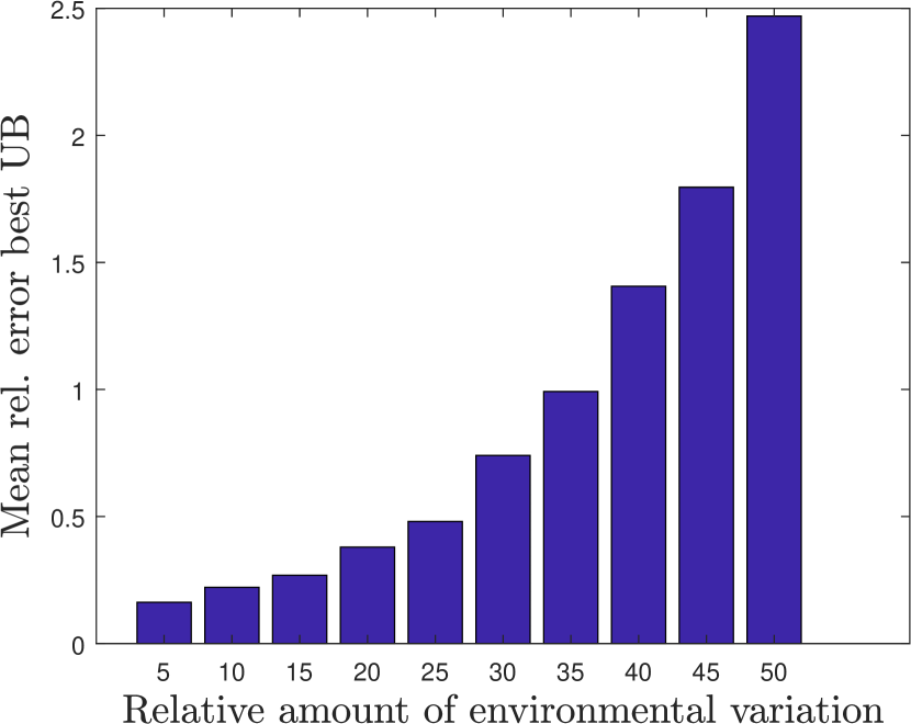
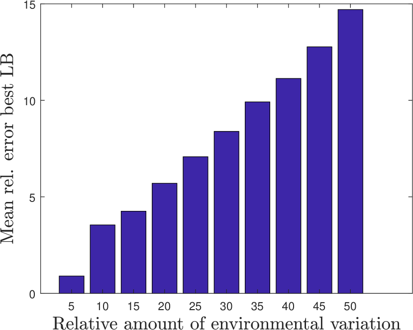
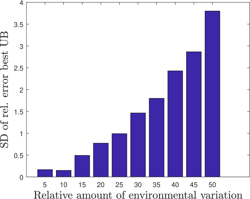
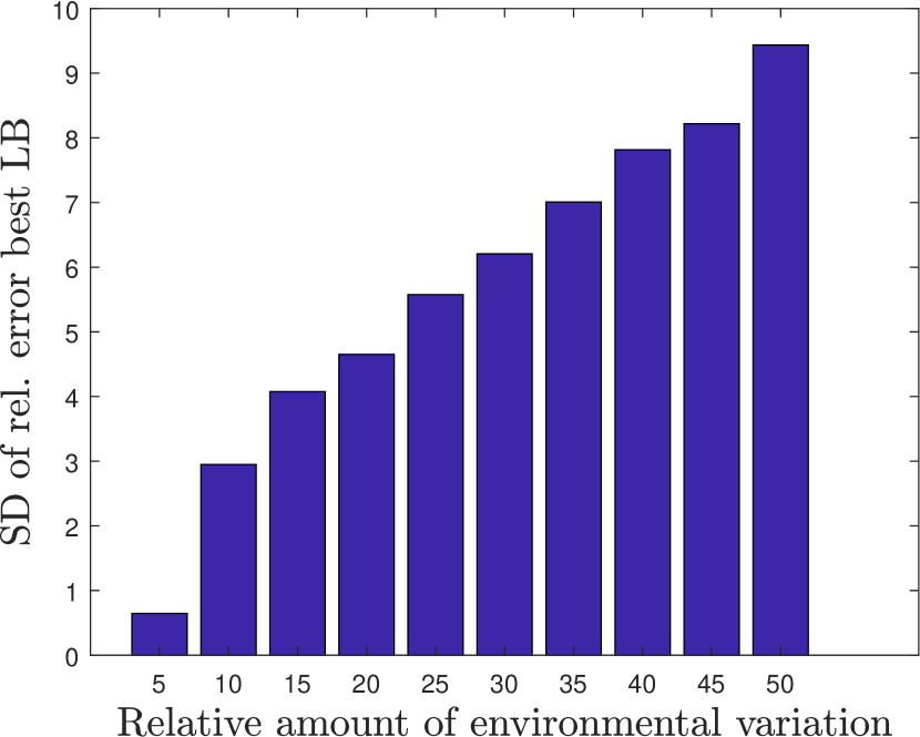
The second question we want to analyze is how large is the relative error incurred when using the best upper or best lower bound for $\lambda_{\mathrm{S}}$. Note that we work with $\lambda_{\mathrm{S}},$ and not with $\log\lambda_{\mathrm{S}},$ to avoid having to divide by numbers close to zero when computing the relative error in the cases for which $\lambda_{\mathrm{S}}$ is close to $1$.

It is reasonable to expect that this error depends strongly on the amount of environmental variation. Therefore, a set of simulations similar to the ones described above has been carried out. We have computed the relative error $100\ast\left|\lambda_{\mathrm{S}}-C\right|/\lambda_{\mathrm{S}},$ where $C$ is the best (upper or lower) bound for $\lambda_{\mathrm{S}}$, and have compared it to the relative amount of environmental variation, measured as

$$100\ast\frac{\left|f_{2}-f_{1}\right|+\left|s_{2}-s_{1}\right|+\left|F_{2}-F_{1}\right|}{\max\left\{f_{1},f_{2}\right\}+\max\left\{s_{1},s_{2}\right\}+\max\left\{F_{1},F_{2}\right\}}.$$

The SGR can not be obtained analytically and, therefore, has been approximated by means of numerical simulations. Specifically, we have used the approach described in tuljapurkar1997stochastic and, in order to keep the computational cost manageable and still obtain a good approximation, be have used $N=$500 samples each of them with a length of $T=$600 time steps. In order to estimate the sampling error for these values of $N$ and $T$ we have compared the results for these values with the ones corresponding to very large values of these parameters, specifically $N=2000$ and $T=8000,$ for which we can expect a very accurate estimate of $\lambda_{\mathrm{S}}$ to be obtained. Thus, we have computed $\lambda_{\mathrm{S}}$ in 100 different cases using both procedures, and have obtained that the maximum discrepancy between them is around 0.3%, whereas the mean discrepancy is around 0.1%. Therefore, we can consider that the sampling error has almost no effect in the estimation of the relative error for the best upper and lower bounds.

The results are shown in Figure 1. They suggest that both the best upper bound and the best lower bound are quite good approximations to the SGR for a wide range of values of environmental variation. They also show that the mean error for the best upper bound is roughly half that corresponding to the best lower bound. Note the comparatively large standard deviation in the distribution of the error corresponding to both the best upper and best lower bound, specially in the latter case.

Figure 1: Mean and standard deviation (SD) of relative error (%) for the best upper bound (UB) and the best lower bound (LB) of $\lambda_{S}$ as functions of relative environmental variation (%)

We conclude this section with some comments about Tuljapurkar’s second order approximation to the SGR $\lambda_{T}$ (Tuljapurkar, 1982) which, as pointed out before, is a popular tool for ecologists. In the previous simulations we have analyzed some properties of $\lambda_{T}$ and have reached interesting conclusions. In the first place, in around 95% of cases $\lambda_{T}$ underestimates the SGR. Secondly, in around 99% of cases $\lambda_{T}$ is larger than the best lower bound. These two points suggest that, as a rule of thumb that works in most situations, we could consider $\lambda_{T}$ as a “practical lower bound” for the SGR (although from a rigorous point of view it is not) that, in many cases, performs better that the lower bounds that have been studied in this work.

7 A study of growth/extinction in a stochastic Leslie model

As an illustration of a practical use of the bounds presented in this work, let us consider the Leslie model with two age classes (4) in the following setting: there are two possible environments, i.e., $\mathcal{I}=\left\{1,2\right\}$. Environment $1$ is rich in the sense that $\rho(\boldsymbol{A}_{1})>1$ whereas environment $2$ is poorer in the sense that the adults fertility is reduced by an amount $\Delta>0$, i.e.,

$$\boldsymbol{A}_{1}:=\left(\begin{array}[c]{cc}f&F\\ s&0\end{array}\right),\ \boldsymbol{A}_{2}:=\left(\begin{array}[c]{cc}f&F-\Delta\\ s&0\end{array}\right).$$

We consider fixed values of $f>0$, $F>0$ and $s\in(0,1],$ with the restriction that $\rho(A_{1})>1$ or alternatively, using the net reproductive value, that

$$f+sF>1.$$ (26)

Therefore, if subjected to environment 1 alone, the population grows to infinity. Let us consider the IID setting, let $\pi_{1}\in(0,1)$ be fixed and let $\boldsymbol{\pi}=\left(\pi_{1},1-\pi_{1}\right)$ be the probability distribution of environmental states.

Clearly, when $\Delta=0,$ we only have environment 1 and the population grows to infinity. Also, as $\Delta$ increases the population fitness decreases. Therefore, we want to answer the following question: what is the maximum value of $\Delta$, that we denote $\Delta_{\text{max}}$, such that $\lambda_{\mathrm{S}}>1$ and so the population does not go extinct? Since the SGR can not be derived analytically, the problem can not be solved directly. Our strategy will be to consider one lower bound for the SGR, say $c<\log\lambda_{\mathrm{S}}$, and to obtain the maximum value $\Delta_{c}$ such that $c(\Delta)>1$ whenever $0<\Delta<\Delta_{c}$. Consequently, if the last inequality holds we know that the population grows to infinity. Note that $\Delta_{c}\leq\Delta_{\text{max}}$, i.e., with this approach we obtain sufficient (but not necessary) conditions on $\Delta$ for population growth. Whenever possible, we want to find closed form expressions for $\Delta_{c}$. In what follows we will complete this process in turn for the different lower bounds for the SGR.

Use of Cohen’s bound $c_{I}$ (11). We distinguish two situations:

• Case a. $F>1$. In that case it is easy to show, using (26), that $f+s<F$. Therefore from (11) one has $c_{I}=\log\left(\left(f+s\right)^{\pi_{1}}\left(F-\Delta\right)^{1-\pi_{1}}\right)$ and therefore $c_{I}>0$ if and only if

  $$\Delta<\Delta_{IA}:=F-\left(f+s\right)^{\frac{\pi_{1}}{\pi_{1}-1}}.$$

• Case b. $F<1$. Then $f+s>F$ and $c_{I}=\log\left(F^{\pi_{1}}\left(F-\Delta\right)^{1-\pi_{1}}\right),$ so $c_{I}>0$ if and only if

  $$\Delta<\Delta_{IB}:=F\left(1-F^{\frac{1}{\pi_{1}-1}}\right).$$

Use of bound $c_{III}$. From (20) it follows that

$$c_{III}=\log\rho(\boldsymbol{A}_{1})+\left(1-\pi_{1}\right)\log\left(1-\frac{\Delta}{F}\right),$$

and so $c_{III}>0$ if and only if

$$\Delta<\Delta_{III}:=F\left(1-\rho(\boldsymbol{A}_{1})^{\frac{1}{\pi_{1}-1}}\right).$$

Use of bound $c_{IV}$. In this case $c_{IV}=c_{\min}=\rho(\boldsymbol{A}_{2}),$ and so $c_{IV}>0$ if and only if $\rho(\boldsymbol{A}_{2})>1$, i.e., if and only if $f+s(F-\Delta)>1$ or, equivalently,

$$\Delta<\Delta_{IV}:=F-\frac{1-f}{s}.$$

One can proceed similarly by working with bound $c_{II}$. A closed form expression of the maximum value of $\Delta$ is not possible using $c_{V}$ due to the complexity of the equation involved.

The question now is to find out, for each value of the model parameters, which lower bound wins, i.e., which of the different lower bounds provides the largest value of $\Delta$ for which one can guarantee non extinction. In order to address this issue, several numerical simulations have been performed that show that, even in this particular setting in which only one parameter varies from environment 1 to environment 2, there is no overall best lower bound, but different lower bounds can win depending on parameters values. Figure 2 shows the values of $\log\lambda_{\mathrm{S}}$ (obtained through numerical simulations) and of the lower bounds as functions of $\Delta$ for three different configurations, that we denote Case A, Case B and Case C. In Case A, $c_{IV}$ wins and the worst bounds are $c_{I}$ for low values of $\Delta$ and $c_{III}$ for larger values. The situation changes dramatically in Case B, for $c_{III}$ becomes the winner, whereas the worst bounds are now $c_{I}$ for low values of $\Delta$ and $c_{IV}$ for larger values. In Case C bound $c_{V}$ wins whereas $c_{I}$ and $c_{III}$ (in this case these two bounds coincide) are the worst.

(a) Case A. $\pi_{1}=0.5$, $F=1.35$, $f=0.55$, $s=0.45.$

(b) Case B. $\pi_{1}=0.9$, $F=1.3$, $f=0.5$, $s=0.5.$

(c) Case C. $\pi_{1}=0.5$, $F=1.1$, $f=0.7$, $s=0.4.$

Figure 2: Values of $\log\lambda_{S}$ and of the lower bounds as a function of $\Delta$ in three different configurations.

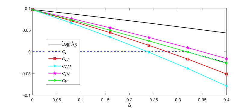
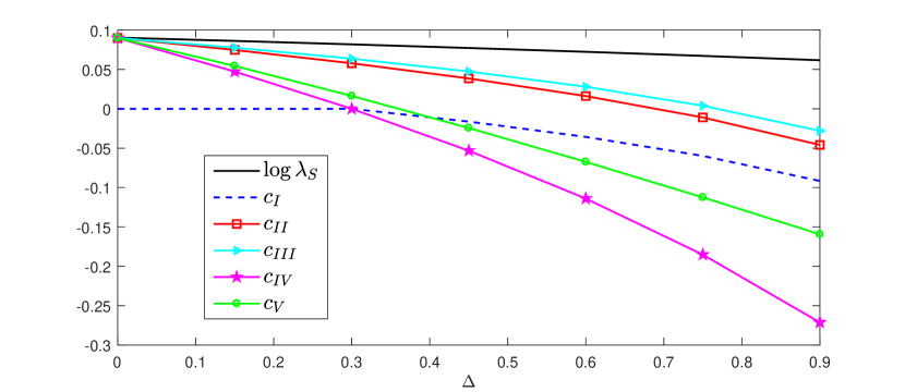
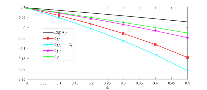
We argued in Section 6 that in most practical cases we can consider $\lambda_{T}$ is a “practical” lower bound for $\lambda_{\mathrm{S}}$. Therefore, we could try, in principle, to find the maximum value of $\Delta$ proceeding as above. However the resulting expression for $\lambda_{T}$ as a function of $\Delta$ is very complicated and so it is not possible to find a closed-form expression for the maximum value of $\Delta$ using $\lambda_{T}$. Numerically, one can observe that in the three cases A, B and C, $\lambda_{T}$ is lower than $\lambda_{\mathrm{S}}$ and that it performs better than the rest of the lower bounds.

8 Discussion and conclusion

Except in very particular cases, the SGR of matrix population models subjected to environmental stochasticity can not be derived analytically. In this work we have introduced four new upper and lower bounds for the SGR. These bounds, which at least for two-stage models are easy derived as close form expressions, can provide both quantitative and qualitative information about ecological models. Specially relevant is the fact that they can be used to give sufficient conditions for population growth or population extinction (see the Introduction and Section 7).

The bounds for the SGR are been obtained following two different strategies. The first one, valid for all kind of models, is a perturbation approach. The second one, useful for Leslie models with two age classes, makes use of certain bounds for the vector of population structure that we have introduced and that generalize previous results in the field.

The different bounds have been analyzed through computer simulations in the context of Leslie models with two age classes. In general, the best upper bound does a better job at approximating $\lambda_{\mathrm{S}}$ than the best lower bounds. As far as the upper bounds are concerned, the rate of growth $\mu$ of the mean population size is the best upper bound for $\lambda_{\mathrm{S}}$ in the vast majority of cases, and so it is the best quick choice for the job. As far as the lower bounds are concerned, there is no clear winner and the best bound depends strongly on the specific parameter values, although a number of general guidelines have been provided. It has also been found that Tuljapurkar’s second order approximation to $\lambda_{\mathrm{S}}$ underestimates $\lambda_{\mathrm{S}}$ in most (but not all) cases and that it usually performs better that the lower bounds that have been studied in this work.

Section 7 illustrates one of the possible applications of the bounds to the study of stochastic population models. There are many more applications in which the bounds can be useful, and we proceed to give some ideas about one of them. Let us consider an age-structured stochastic model like that of Section 2.1 with two environments. In the first environment the dominant eigenvalue of the corresponding PPM is greater that one whereas in the case of the second environment it is less that one. By using one lower bound and proceeding like in Section 7, we can find a value $\pi^{\ast}\in(0,1)$ such that if the asymptotic probability $\pi_{1}$ of environment one verifies $\pi_{1}>\pi^{\ast}$ then the population grows to infinity. Similarly, the use of an upper bound allows one to find a value $\hat{\pi}\in(0,1)$ such that the population goes extinct whenever $\pi_{1}<\hat{\pi}$.

9

Appendix A Matrix models with environmental stochasticity

The following theorem summarizes some results in the literature (Furstenberg and Kesten, 1960; Cohen, 1977; Tuljapurkar and Orzack, 1980) about the dynamics of models of the kind (2) which are relevant in this work:

Theorem 1.

Let us consider system (2) and assume that:

a. The set $\{\boldsymbol{A}_{\eta},\ \eta\in\mathcal{I}\}$ of vital rates matrices is ergodic, i.e., there exists a positive integer $g$ such that any product of $g$ matrices (with repetitions allowed) drawn from $\mathcal{A}$ is a positive matrix (i.e., its components are all positive) and, moreover, there exist constants $\alpha,\beta>0$ such that for all $\eta\in\mathcal{I}$

$$\max(\boldsymbol{A}_{\eta})\leq\beta\ \ ;\ \ \min\nolimits^{+}(\boldsymbol{A}_{\eta})\geq\alpha,$$

where $\max(\boldsymbol{A}_{\eta})$ is the maximum of the elements of $\boldsymbol{A}_{\eta}$ and $\min^{+}(\boldsymbol{A}_{\eta})$ is the minimum of the positive elements of $\boldsymbol{A}_{\eta}$. Clearly, when $\mathcal{I}$ is finite, the second condition can be omitted.

b. $\tau_{t}$ is a homogeneous Markov chain that has an unique stationary distribution, and the transition probabilities of $\tau_{t}$ converge geometrically to it. When $\mathcal{I}$ is finite, a sufficient condition for this is that $\tau_{t}$ be an homogeneous irreducible and aperiodic homogeneous Markov chain.

Then:

1. The joint process $\left(\tau_{t},\boldsymbol{z}(t)/\left\|\boldsymbol{z}(t)\right\|\right)$ is a Markov chain that converges to a stationary distribution $G$.

2. We can define the stochastic growth rate (SGR) $\lambda_{\mathrm{S}}$ of system (2) through $\log\lambda_{\mathrm{S}}:=\underset{t\rightarrow\infty}{\lim}\log\left\|\boldsymbol{z}(t)\right\|/t$ where the limit holds with probability one. Moreover, $\lambda_{\mathrm{S}}$ is finite, is independent of the initial probabilities of $\tau_{t}$ and of the initial (non-zero) population vector $\boldsymbol{z}_{0}\geq\mathbf{0}$ and can be calculated through

$$\log\lambda_{\mathrm{S}}=\mathbb{E}_{G}\log\left\|\boldsymbol{A}_{\tau_{t+1}}\frac{\boldsymbol{z}(t)}{\left\|\boldsymbol{z}(t)\right\|}\right\|,$$ (27)

where the expectation is taken with respect to the stationary distribution $G$.

Appendix B Proofs

Proof of the bounds (18). Following (Furstenberg and Kesten, 1960; Tuljapurkar and Orzack, 1980) the SGR of system (2) can be calculated through any of the components of the matrix product, i.e., for all $i,j=1,...,n$ we have

$$\log\lambda_{\mathrm{S}}=\lim_{t\rightarrow\infty}\log\left(\boldsymbol{A}_{\tau_{t}}\boldsymbol{A}_{\tau_{t-1}}\cdots\boldsymbol{A}_{\tau_{2}}\boldsymbol{A}_{\tau_{1}}\right)^{ij}/t,$$ (28)

with probability one.

From (15) we can write $A_{\eta}^{ij}=\left(1+W_{\eta}^{ij}\right)B_{\eta}^{ij}$ for all $\eta\in\mathcal{I}$ and $i,j=1,...,n,$ and therefore for all $i,j=1,...,n$ one has

$$\left(\boldsymbol{A}_{\tau_{t}}\boldsymbol{A}_{\tau_{t-1}}\cdots\boldsymbol{A}_{\tau_{2}}\boldsymbol{A}_{\tau_{1}}\right)^{ij}\leq$$

$$\leq\left(1+W_{\tau_{t}}^{M}\right)\left(1+W_{\tau_{t-1}}^{M}\right)\cdots\left(1+W_{\tau_{2}}^{M}\right)\left(1+W_{\tau_{1}}^{M}\right)\left(\boldsymbol{B}_{\tau_{t}}\boldsymbol{B}_{\tau_{t-1}}\cdots\boldsymbol{B}_{\tau_{2}}\boldsymbol{B}_{\tau_{1}}\right)^{ij},$$

from where it follows

$$\frac{\log\left(\boldsymbol{A}_{\tau_{t}}\boldsymbol{A}_{\tau_{t-1}}\cdots\boldsymbol{A}_{\tau_{2}}\boldsymbol{A}_{\tau_{1}}\right)^{ij}}{t}\leq$$ (29)

$$\frac{\log\left[\left(1+W_{\tau_{t}}^{M}\right)\left(1+W_{\tau_{t-1}}^{M}\right)\cdots\left(1+W_{\tau_{2}}^{M}\right)\left(1+W_{\tau_{1}}^{M}\right)\right]}{t}+\frac{\log\left(\boldsymbol{B}_{\tau_{t}}\boldsymbol{B}_{\tau_{t-1}}\cdots\boldsymbol{B}_{\tau_{2}}\boldsymbol{B}_{\tau_{1}}\right)^{ij}}{t}.$$

Let us consider the scalar system

$$x(t+1)=\left(1+W_{\tau_{t+1}}^{M}\right)x(t).$$ (30)

Since, according to (17), we have $1+W_{\eta}^{M}>0$ for all $\eta\in\mathcal{I}$, the set $\left\{1+W_{\eta}^{M},\eta\in\mathcal{I}\right\}$ is ergodic and therefore system (30) has a SGR. In order to calculate it, we use (27) and take into account that, since the system is scalar, the process $x(t)/\left\|x(t)\right\|$ is trivial (equals 1 with probability one). So the joint distribution of $\left(\tau_{t},x(t)/\left\|x(t)\right\|\right)$ coincides with the distribution of $\tau_{t}$ and so

$$\lim_{t\rightarrow\infty}\frac{\log\left[\left(1+W_{\tau_{t}}^{M}\right)\left(1+W_{\tau_{t-1}}^{M}\right)\cdots\left(1+W_{\tau_{2}}^{M}\right)\left(1+W_{\tau_{1}}^{M}\right)\right]}{t}=\underset{\eta\in\mathcal{I}}{\sum}\pi_{\eta}\log\left(1+W_{\eta}^{M}\right).$$ (31)

From (28) it follows that $\lim_{t\rightarrow\infty}\log\left(\boldsymbol{A}_{\tau_{t}}\boldsymbol{A}_{\tau_{t-1}}\cdots\boldsymbol{A}_{\tau_{2}}\boldsymbol{A}_{\tau_{1}}\right)^{ij}/t=\log\lambda_{\mathrm{S}}$ and $\lim_{t\rightarrow\infty}\log\left(\boldsymbol{B}_{\tau_{t}}\boldsymbol{B}_{\tau_{t-1}}\cdots\boldsymbol{B}_{\tau_{2}}\boldsymbol{B}_{\tau_{1}}\right)^{ij}/t=\log\lambda_{\mathrm{S}}^{\prime}$. Using this facts, together with (31), in (29) we finally obtain

$$\log\lambda_{\mathrm{S}}\leq\log\lambda_{\mathrm{S}}^{\prime}+\underset{\eta\in\mathcal{I}}{\sum}\pi_{\eta}\log\left(1+W_{\eta}^{M}\right).$$

The other inequality in (18) follows from an analogous reasoning substituting the upper bound in (29) by the corresponding lower bound.

Proof of bounds (24) for population structure. To start with, since we are only interested in age structure, in matrices $\boldsymbol{A}_{\eta}$ we can factor out the fertility of the young, i.e.,

$$\boldsymbol{A}_{\tau_{t}}=f_{\tau_{t}}\begin{pmatrix}1&\varepsilon_{t}\\ \gamma_{t}&0\end{pmatrix},$$

where we have defined

$$\varepsilon_{t}:=F_{\tau_{t}}/f_{\tau_{t}},\ \gamma_{t}:=s_{\tau_{t}}/f_{\tau_{t}},$$

and we proceed to work with matrices

$$\begin{pmatrix}1&\varepsilon_{t}\\ \gamma_{t}&0\end{pmatrix}.$$

We use the same reasoning of Tuljapurkar in (Tuljapurkar, 1990), and the equivalent to his equation (8.1.3) reads

$$\frac{z^{2}(t+1)}{z^{1}(t+1)}=\frac{\gamma_{t+1}}{1+\varepsilon_{t+1}\frac{z^{2}(t)}{z^{1}(t)}}=:f_{t+1}(z^{2}(t)/z^{1}(t)),$$

where function $f_{t+1}$ is increasing as a function of $\gamma_{t+1}$, decreasing as a function of $\varepsilon_{t+1}$ and decreasing as a function of $z^{2}(t)/z^{1}(t)$. From the first two assertions if follows that, if we define for each value of $z^{2}(t)/z^{1}(t)$

$$f_{\min}(z^{2}(t)/z^{1}(t)):=\frac{\gamma_{m}}{1+\varepsilon_{M}\frac{z^{2}(t)}{z^{1}(t)}},\text{ }f_{\max}(z^{2}(t)/z^{1}(t)):=\frac{\gamma_{M}}{1+\varepsilon_{m}\frac{z^{2}(t)}{z^{1}(t)}},$$

one has

$$f_{\min}(z^{2}(t)/z^{1}(t))\leq f_{t+1}(z^{2}(t)/z^{1}(t))\leq f_{\max}(z^{2}(t)/z^{1}(t)).$$

From here, and reasoning as in (Tuljapurkar, 1990, Section 8.1), we obtain that, for any initial vector and large enough $t$, the expression $\delta\leq z^{2}(t)/z^{1}(t)\leq\kappa$ holds where

$$\delta=\lim_{t\rightarrow\infty}\delta(t),\ \ \kappa=\lim_{t\rightarrow\infty}\kappa(t),$$ (32)

and $\delta(t)$ and $\kappa(t)$ are defined iteratively through

$$\delta(1) =(f_{\min}\circ f_{\max})(z^{2}(0)/z^{1}(0)),...,\ \delta(t)=(f_{\min}\circ f_{\max})(\delta(t-1))$$ (33)

$$\kappa(1) =(f_{\max}\circ f_{\min})(z^{2}(0)/z^{1}(0)),...,\ \kappa(t)=(f_{\max}\circ f_{\min})(\kappa(t-1)).$$

The dynamics of $\delta(t)$ can be studied as follows: Let

$$\boldsymbol{X}_{\min}=\begin{pmatrix}1&\varepsilon_{M}\\ \gamma_{m}&0\end{pmatrix},\text{ \ \ \ \ }\boldsymbol{X}_{\max}=\begin{pmatrix}1&\varepsilon_{m}\\ \gamma_{M}&0\end{pmatrix},$$

and take any positive initial vector $\boldsymbol{z}(0).$ If we apply matrix $\boldsymbol{X}_{\max}$ to $\boldsymbol{z}(0)$ and then $\boldsymbol{X}_{\min}$, the new population vector verifies that the ratio of adult to young is given by $(f_{\min}\circ f_{\max})(z^{2}(0)/z^{1}(0))$. Therefore, from (32) and (33) we have $\delta=v^{2}/v^{1},$ where $\boldsymbol{v}=(v^{1},v^{2})$ is the dominant eigenvector of matrix

$$\boldsymbol{X}_{\min}\boldsymbol{X}_{\max}=\begin{pmatrix}1+\varepsilon_{M}\gamma_{M}&\varepsilon_{m}\\ \gamma_{m}&\gamma_{m}\varepsilon_{m}\end{pmatrix}.$$

Straightforward computations show that $\delta$ has indeed the expression given by (24).

Regarding $\kappa,$ the same reasonings above apply replacing product $\boldsymbol{X}_{\min}\boldsymbol{X}_{\max}$ by $\boldsymbol{X}_{\max}\boldsymbol{X}_{\min}$.

Proof of bounds (25). We make use of (27) and therefore

$$\mathbb{E}_{G}\log\left\|\boldsymbol{A}_{\tau_{t+1}}\frac{\boldsymbol{z}(t)}{\left\|\boldsymbol{z}(t)\right\|}\right\| =\mathbb{E}_{G}\log\left(\overset{n}{\underset{i=1}{\sum}}\overset{n}{\underset{j=1}{\sum}}A_{\tau_{t+1}}^{ij}\frac{z^{j}(t)}{\left\|\boldsymbol{z}(t)\right\|}\right)\leq\mathbb{E}_{G}\log\left(\overset{n}{\underset{i=1}{\sum}}\overset{n}{\underset{j=1}{\sum}}u_{\eta}^{j}A_{\tau_{t+1}}^{ij}\right)=$$

$$=\mathbb{E}_{G}\log\left(\overset{n}{\underset{j=1}{\sum}}u_{\eta}^{j}\overset{n}{\underset{i=1}{\sum}}A_{\tau_{t+1}}^{ij}\right)=\mathbb{E}_{G}\log\left(\overset{n}{\underset{j=1}{\sum}}u_{\eta}^{j}\varphi_{\tau_{t+1}}^{j}\right)=$$

$$=\underset{\eta\in\mathcal{I}}{\sum}\pi_{\eta}\log\left(\overset{n}{\underset{j=1}{\sum}}u^{j}\varphi_{\eta}^{j}\right),$$

where in the last equality we have used that we are taking the expected value of a random variable that is independent of the population structure $\boldsymbol{z}(t)/\left\|\boldsymbol{z}(t)\right\|$. Thus, the expression of $C_{IV}$ has been obtained. An analogous reasoning leads to the expression of $c_{IV}$.

Acknowledgements

Author is supported by Ministerio de Economía y Competitividad (Spain), Project MTM2014-56022-C2-1-P.

References

- Alonso and Sanz [2009] Alonso, J.A., Sanz, L., 2009. Approximating the distribution of population size in stochastic multiregional matrix models with fast migration. Philosophical Transactions of the Royal Society A: Mathematical, Physical and Engineering Sciences 367, 4801–4827.
- Billingsley [2008] Billingsley, P., 2008. Probability and measure. John Wiley & Sons.
- Caswell [2001] Caswell, H., 2001. Matrix Population Models: Construction, analysis, and interpretation. Sunderland: Sinauer.
- Cohen [1977] Cohen, J.E., 1977. Ergodicity of age structure in populations with markovian vital rates. ii. general states. Advances in Applied Probability 9, 18–37.
- Cohen [1979] Cohen, J.E., 1979. Long-run growth rates of discrete multiplicative processes in markovian environments. Journal of Mathematical Analysis and Applications 69, 243–251.
- Compagnoni et al. [2016] Compagnoni, A., Bibian, A.J., Ochocki, B.M., Rogers, H.S., Schultz, E.L., Sneck, M.E., Elderd, B.D., Iler, A.M., Inouye, D.W., Jacquemyn, H., et al., 2016. The effect of demographic correlations on the stochastic population dynamics of perennial plants. Ecological Monographs 86, 480–494.
- Cushing and Yicang [1994] Cushing, J., Yicang, Z., 1994. The net reproductive value and stability in matrix population models. Natural Resources Modeling 8, 297–333.
- Davison et al. [2013] Davison, R., Nicolè, F., Jacquemyn, H., Tuljapurkar, S., 2013. Contributions of covariance: decomposing the components of stochastic population growth in cypripedium calceolus. The American Naturalist 181, 410–420.
- Furstenberg and Kesten [1960] Furstenberg, H., Kesten, H., 1960. Products of random matrices. The Annals of Mathematical Statistics 31, 457–469.
- Gremer and Venable [2014] Gremer, J.R., Venable, D.L., 2014. Bet hedging in desert winter annual plants: optimal germination strategies in a variable environment. Ecology letters 17, 380–7. doi:10.1111/ele.12241.
- McDonald et al. [2016] McDonald, J.L., Stott, I., Townley, S., Hodgson, D.J., 2016. Transients drive the demographic dynamics of plant populations in variable environments. Journal of Ecology 104, 306–314.
- Protasov and Jungers [2013] Protasov, V.Y., Jungers, R., 2013. Lower and upper bounds for the largest lyapunov exponent of matrices. Linear Algebra and its Applications .
- Sanz and Alonso [2010] Sanz, L., Alonso, J., 2010. Approximate aggregation methods in discrete time stochastic population models. Mathematical Modelling of Natural Phenomena 5, 38–69.
- Sanz and Bravo de la Parra [2007] Sanz, L., Bravo de la Parra, R., 2007. Approximate reduction of multiregional models with environmental stochasticity. Mathematical biosciences 206, 134–154.
- Tuljapurkar and Orzack [1980] Tuljapurkar, S., Orzack, S.H., 1980. Population dynamics in variable environments i. long-run growth rates and extinction. Theoretical Population Biology 18, 314–342.
- Tuljapurkar [1982] Tuljapurkar, S.D., 1982. Population dynamics in variable environments. iii. evolutionary dynamics of r-selection. Theoretical Population Biology 21, 141–165.
- Tuljapurkar [1990] Tuljapurkar, S.D., 1990. Population dynamics in variable environments. Berlin: Springer Verlag.
- Williams et al. [2015] Williams, J.L., Jacquemyn, H., Ochocki, B.M., Brys, R., Miller, T.E., 2015. Life history evolution under climate change and its influence on the population dynamics of a long-lived plant. Journal of Ecology 103, 798–808.