Learning a Decision Tree Algorithm with Transformers

Abstract

Decision trees are renowned for their interpretability capability to achieve high predictive performance, especially on tabular data. Traditionally, they are constructed through recursive algorithms, where they partition the data at every node in a tree. However, identifying the best partition is challenging, as decision trees optimized for local segments may not bring global generalization. To address this, we introduce MetaTree, which trains a transformer-based model on filtered outputs from classical algorithms to produce strong decision trees for classification. Specifically, we fit both greedy decision trees and optimized decision trees on a large number of datasets. We then train MetaTree to produce the trees that achieve strong generalization performance. This training enables MetaTree to not only emulate these algorithms, but also to intelligently adapt its strategy according to the context, thereby achieving superior generalization performance.

1 Introduction

(A) Depth-2 trees	(B) Depth-3 trees

(C) Tree of Prompts dataset

Figure 1: MetaTree demonstrates strong generalization on real-world datasets. MetaTree generalizes well to 91 held-out datasets for both (A) depth-2 trees and (B) depth-3 trees, despite only being trained to produce depth-2 trees. (C) MetaTree also generalizes well to the 13 Tree-of-prompts datasets which require constructing a tree to steer a large language model (Morris et al., 2023). Each plot shows the average test accuracy for tree ensembles of size {1, 5, 10, 20, 30, 40, 50, 60, 70, 80, 90, 100}, with error bars indicating the standard deviation.

Figure 2: The creation of a decision tree, depicted in (a), entails recursive MetaTree calls. MetaTree only assesses the current state for its decision-making. (b) shows MetaTree’s tabular attention mechanism, in which the tabular input is processed with row and column attention at each layer, and the output is a one-hot mask indicating the splitting feature $j$ and threshold $\mathrm{X}_{i,j}$.

Transformers (Vaswani et al., 2017) have demonstrated the capacity to generate accurate predictions on tasks previously deemed impossible (OpenAI, 2023; Betker et al., 2023), but can they produce models rather than predictions? In this work, we study whether Transformers can generate a particular class of models: decision trees. We select decision trees as they are foundational building blocks of modern machine learning and hierarchical reasoning. They offer interpretability, which modern deep learning models often sacrifice, while maintaining state-of-the-art performance across a wide range of practical applications (Grinsztajn et al., 2022).

Traditionally, decision trees are constructed using algorithms based on greedy heuristics (Breiman et al., 1984; Quinlan, 1986). To overcome the bias imposed by greedy algorithms, recent work has proposed optimal, discrete optimization methods for fitting decision trees (Lin et al., 2020; Hu et al., 2019; Bertsimas & Dunn, 2017). However, the task of full decision tree optimization is NP-hard (Laurent & Rivest, 1976), rendering it practically infeasible to compute optimal trees with large tree depths. While these approaches have been effective in tabular contexts, a significant challenge lies in their non-differentiability, which raises difficulties when integrating them into deep learning models.

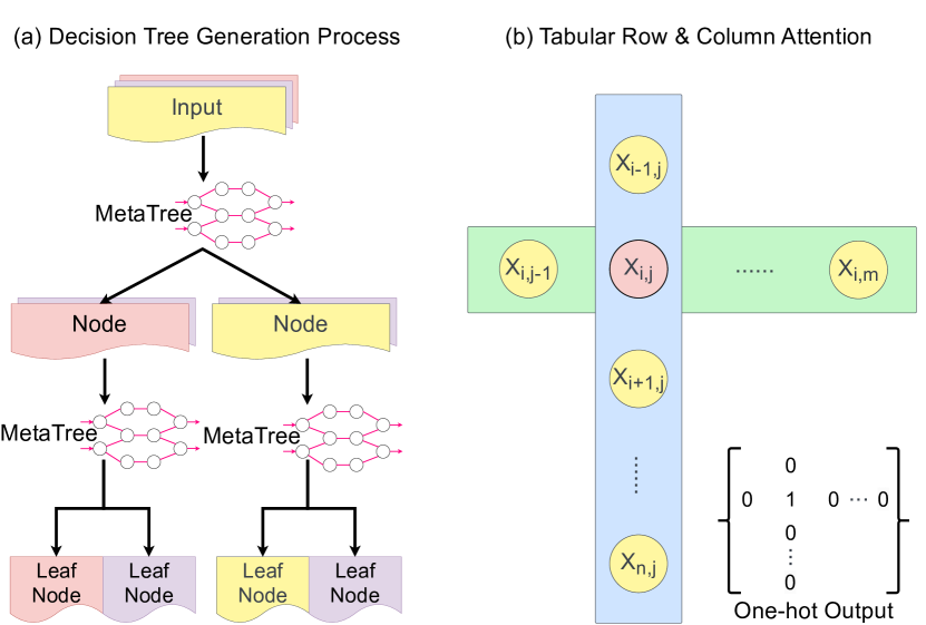
In this work, we introduce MetaTree, a Transformer model designed to construct a decision tree given a tabular dataset. MetaTree recursively applies a Transformer to decide the splitting feature and value for each decision node (Fig. 2a). We train MetaTree to produce high-performing decision trees given a new dataset. Specifically, we fit both greedy decision trees and optimized decision trees on a large number of datasets. We then train MetaTree to generate the trees that demonstrated superior generalization performance. This training strategy endows MetaTree with a unique advantage: it learns not just to mimic the construction process of these algorithms but also to discern when to lean towards each algorithmic approach based on the specific context of the dataset. This adaptability add significant flexibility to traditional methods that are bound to a single algorithmic framework. MetaTree’s architecture leverages an alternating row and column attention mechanism along with a learnable absolute positional bias for the tabular representations.

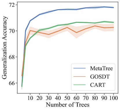
MetaTree produces highly predictive trees on a large set of real-world datasets that it did not see during training, consistently outperforming traditional decision tree algorithms (Fig. 1). Additionally, MetaTree demonstrates resilience to noise and can generalize to problems involving high-order interactions. Further analysis shows that MetaTree’s performance improvement comes from its ability to dynamically switch between a greedy or global approach depending on the context of the dataset. Finally, a bias-variance analysis shows that MetaTree successfully achieves lower empirical variance than traditional decision-tree algorithms.

2 Related work

Decision trees

There is a long history of greedy methods for fitting decision trees, e.g., CART (Breiman et al., 1984), ID3 (Quinlan, 1986), or C4.5 (Quinlan, 2014). Recent work has explored fitting trees overcoming greedy heuristics via global optimization (Lin et al., 2020; Hu et al., 2019; Bertsimas & Dunn, 2017); this can improve performance given a fixed tree size but often incurs a prohibitively high computational cost. Other recent studies have improved trees through regularization (Agarwal et al., 2022), iterative updates (Carreira-Perpinán & Tavallali, 2018), or increased flexibility (Tan et al., 2022).

Trees maintain state-of-the-art performance across tabular applications (Grinsztajn et al., 2022; Kornblith et al., 2022), especially when used in ensembles such as Random Forest (Breiman, 2001), gradient-boosted trees (Freund et al., 1996), and BART (Chipman et al., 2010). Some recent works have studied the intersection of trees and transformers, e.g. using trees to guide LLM generations (Morris et al., 2023; Yao et al., 2023) or, conversely, using LLMs to build stronger decision trees for text classification (Singh et al., 2023).

Learning models/algorithms

Some learning-based methods have focused on improving algorithms, largely based on combining Transformers with deep reinforcement learning, e.g. faster matrix multiplication (Fawzi et al., 2022) or faster sorting algorithms (Mankowitz et al., 2023). One new work studies using LLMs to iteratively generate and refine code to discover improved solutions to problems in computer science and mathematics (Romera-Paredes et al., 2023).

Other works focus on Transformers’ ability to learn in context. Zhou et al. (2023) probe simple tasks for length generalization and find that Transformers can generalize to a certain class of problems easily. One very related work studies whether Transformers can successfully learn to generate predictions from linear functions, and even decision trees and small MLPs in context (Garg et al., 2022). Despite these successes, recent works also find limitations in Transformers’ ability to generalize in certain contexts, e.g. to distribution shifts (Yadlowsky et al., 2023) or to arithmetic (Dziri et al., 2023).

Meta-learning

Often referred to as “learning-to-learn”, meta-learning has gained increasing attention over the years (Nichol et al., 2018; Hospedales et al., 2021). Meta-learning algorithms are designed to learn a model that works well on an unseen dataset/task given many instances of datasets/tasks (Vilalta & Drissi, 2002). Particularly related to MetaTree are works that apply meta-learning with transformers to tabular data (Hollmann et al., 2022; Feuer et al., 2023; Onishi et al., 2023; Hegselmann et al., 2023; Gorishniy et al., 2023; Manikandan et al., 2023; Zhu et al., 2023). While echoing the essence of meta-learning, our objective is to introduce a a learning-based model capable of directly outputting a model informed by the insights of established algorithms.

3 Methods: MetaTree

Figure 3: MetaTree’s training involves a two-phase learning curriculum: in the first phase, the focus is exclusively on learning from the optimized GOSDT trees, to closely emulate the behavior of GOSDT algorithm. Then in the second phase, the training process incorporates data from both the GOSDT and CART trees, generating the ones that have better generalization capabilities.

Problem definition

When generating a decision tree, we are given a dataset $D={(x_{i},y_{i})}_{i=1}^{n}$ where $x_{i}\in\mathbb{R}^{m}$ represents the input features and $y_{i}\in\{1,\ldots,K\}$ corresponds to the label for each instance. At each node, a decision tree identifies a split consisting of a feature $j\in\{1,\ldots,m\}$ and a threshold $v\in\mathbb{R}$, such that $D$ can be partitioned into two subsets by thresholding the value of the $j^{th}$ feature. The dataset is partititioned recursively until meeting a pre-specified stopping criterion, here a maximum tree depth. To generate a prediction, a point is passed through the tree until reaching a leaf node, where the predicted label is the majority label of training points that fall into that leaf node.

Generating a decision tree

Decision trees are typically fit using a top-down greedy algorithm such as CART (Breiman et al., 1984). These algorithms greedily select the split at each node based on a criterion such as the Gini impurity. This class of methods, while efficient, often results in sub-optimal solutions. More recent work has studied the generation of “optimal” decision trees seeking a solution that maximizes predictive performance subject to minimizing the total number of splits in a tree. This can be formulated as a tree search, in which recursive revisions on the tree happen when all children of a search node are proven to be non-optimal (Lin et al., 2020). However, finding optimal trees is intractable for even modest tree depths, and can also quickly overfit to noisy data.

We aim to bridge these approaches with MetaTree to yield highly predictive decision trees as illustrated in Fig. 2(a). To generate a single tree, a recursive call is made to MetaTree at each tree node. Initially, the entire dataset is presented to the model, which makes a partition to form the root node. Then, the dataset is filtered into two subsets by the root node; each subset (i.e. the left child subset and the right child subset) is passed through the model individually, with the opposite subset being masked out. This process is repeated until a maximum depth for the tree is reached. Even though MetaTree only outputs a single split at a time, the fact that it can see the entire dataset and use multiple Transformer layers allows it to make adaptive, non-greedy splits.

Representing numerical inputs

MetaTree takes matrices of real-valued numbers as input. We use a multiplicative embedding to project all the numerical features into embedding space and add the class embedding onto it. The aggregated embedding is then transformed via a two-layer MLP. Specifically, given a n-row m-column input $X\in\mathbb{R}^{n,m}$ and its k-class label $Y\in\{1,\ldots,k\}^{n}$, with $Y_{oh}$ denotes $Y$ in one-hot format, the embedding is computed as follows:

$$\mathrm{Emb_{x}}(X)=X\otimes W_{x}\in\mathbb{R}^{n,m,d},\quad W_{x}\in\mathbb{R}^{d}$$ (1)

$$\mathrm{Emb_{y}}(Y)=Y_{oh}\cdot W_{y}\in\mathbb{R}^{n,d},\quad W_{y}\in\mathbb{R}^{k,d}$$ (2)

$$\mathrm{Emb}=\mathrm{MLP}(\mathrm{Emb_{x}}(X)+\mathrm{Emb_{y}}(Y)+b_{1}+b_{2})$$

$$\mathrm{Emb}\in\mathbb{R}^{n,m,d},\quad b_{1}\in\mathbb{R}^{m,d},\;b_{2}\in\mathbb{R}^{n,d}$$ (3)

For each number in the matrix $X$, it is transformed into $\mathbb{R}^{d}$ space via multiplication with $W_{x}$, then added to the class embedding of $Y$. The final embedding is obtained by putting the aggregated embedding plus the positional bias terms $b_{1},b_{2}$ through an MLP.

We normalize each feature dimension per batch to have mean of 0 and variance of 1. Prior to inference, we also add a truncated Gaussian noise to categorical features; this improves performance on discrete features since the model is mostly trained on continuous data.

Tabular self-attention

Since our tabular input share information across rows and columns, we apply attention to both the row dimension and column dimension in each Transformer layer. Given input in hidden space $X_{h}\in\mathbb{R}^{n,m,d}$, the output of the tabular attention $Y_{h}\in\mathbb{R}^{n,m,d}$ is computed as:

$$\text{ColAttn}(X_{h})=\text{Softmax}(Q_{\text{col}}^{\top}K_{\text{col}})V_{\text{col}}$$ (4)

$$\text{RowAttn}(X_{h})=\text{Softmax}(Q_{\text{row}}^{\top}K_{\text{row}})V_{\text{row}}$$ (5)

$$Y_{h}=\text{ColAttn}(X_{h})+\text{RowAttn}(X_{h})+X_{h}$$ (6)

Attention is applied in the row and column dimensions individually, it will first gather information over $n$ rows and then over $m$ columns with a $O(n^{2}+m^{2})$ complexity. This alleviates the computing cost compared to reshaping the table as a long sequence, which would require a $O\left(n^{2}m^{2}\right)$ complexity, while effectively gathering and propagating information for the entire table.

3.1 Cross entropy with Gaussian smoothing

The main task of our model is to select a feature and value to split the input data. This process involves selecting a specific element from the input matrix $X\in\mathbb{R}^{n,m}$. Suppose the choice is made for $X_{i,j}$, it is equivalent to a decision that splits the data along the $j^{th}$ feature with value $X_{i,j}$. Our design for the model’s output and the corresponding loss function is based on this fundamental principle of split selection. The model’s output is passed through a linear projection to scale down from $\mathbb{R}^{n,m,d}$ to $\mathbb{R}^{n,m,1}$, and the final output is obtained after a Sigmoid activation.

We train our model with supervised learning. In the ground truth tree, each node contains the feature index and the splitting value. This is equivalent to a one-hot mask over the input table where the optimal choice of feature and value is marked as one and the rest marked as zero. However, directly taking this mask as the training signal raises issues: some data points might have similar or exactly the same values along the same feature as the optimal split, and masking out these data points would deeply confuse the model. Hence we use a Gaussian smoothing over this mask as our loss target based on the value distance over the chosen feature, we denote the ground truth splitting feature and value as $j^{*}$ and $v^{*}$, the training target $M$:

$$M=\begin{cases}\exp{-\frac{(X[:,j]-v^{*})^{2}}{2\sigma^{2}}},&\text{if }j=j^{*}\\ 0,&\text{if }j\neq j^{*}\\ \end{cases}$$ (7)

where $\sigma$ is a hyperparameter, controlling the smoothing radius. We use Binary Cross Entropy (BCE) to calculate the loss between our model output and the training target $M$.

Learning curriculum

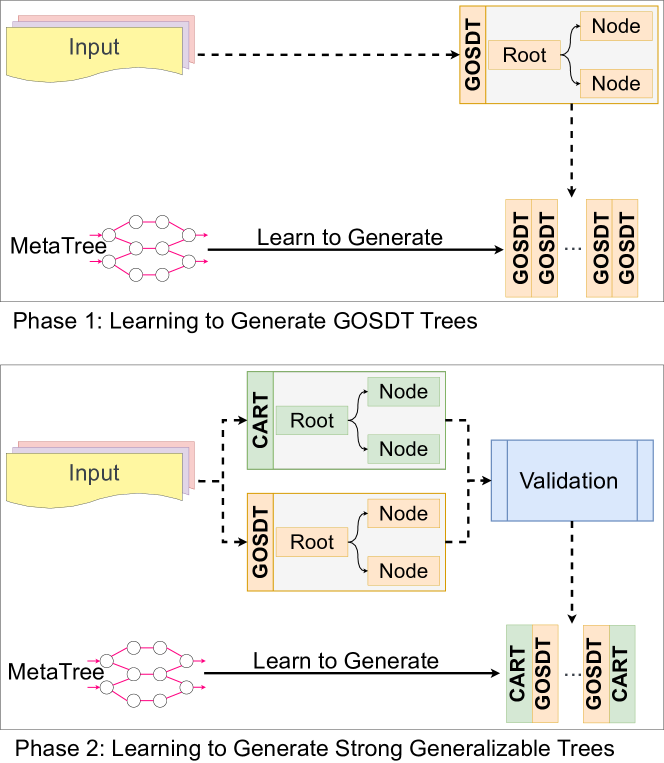
Our training approach is tailored to accommodate the mixed learning signals derived from the two distinct algorithms, each with its unique objectives and behaviors. The task is difficult. Mimicking the optimal decision tree algorithm is already challenging (i.e. approximating solutions for an NP-hard problem), but MetaTree must also learn to generate the split that has a better generalization potential.

To effectively train our model, we use a learning curriculum in our experiments (as illustrated in Fig. 3). In the first phase, the focus is exclusively on learning from the optimal GOSDT trees. The goal during this stage is to closely emulate the behavior of GOSDT algorithm. Then in the second phase, the training process incorporates data from both the GOSDT and CART trees (see details in Sec. 4.1) to train MetaTree. This two-stage approach enables our model to assimilate the characteristics of both algorithms, facilitating better generalization capabilities. (See Sec. A.3 for ablation studies on the training curriculum.)

4 Experimental setup

4.1 Datasets

We use 632 classification datasets from OpenML (Vanschoren et al., 2013), Penn Machine Learning Benchmarks (Romano et al., 2021), along with a synthetic XOR dataset. We require each dataset to have at least 1000 data points, at most 256 features, at most 10 classes, and less than 100 categorical features, with no missing data. We randomly select 91 datasets as the left-out test set for evaluating our model’s generalization capability while making sure they and their variants do not appear in the training set.

We generate our decision-tree training dataset in the following manner: for each dataset, we first divide it into train and test sets with a 70:30 split; then we sample 256 data points with 10 randomly selected feature dimensions from the training set and fit a GOSDT tree (Lin et al., 2020) and a CART tree (Breiman et al., 1984); we later record the accuracy of the two trees on the test set; in the end, we go back to sampling another set of 256 data points to generate 10k trees for each dataset. In total, we have 10,820,000 trees generated for training.

We have both GOSDT and CART trees generated for all these datasets; for clarity, we refer to the GOSDT trees as the GOSDT dataset, the CART trees as the CART dataset, and the trees that have the best evaluation accuracy on their respective test set between CART and GOSDT as the GOSDT+CART dataset.

We additionally test MetaTree on the 13 Tree-of-prompt datasets from Morris et al. (2023). They are tabular datasets constructed from text classification tasks; the input $X$ is the LLM’s response to a set of prompts accompanying the text (yes or no), and the output $Y$ is the class label. Successfully building trees on these datasets shows the potential for MetaTree to help in steering large language models. Moreover, since MetaTree is differentiable, it could be integrated directly into the training process of some LLMs.

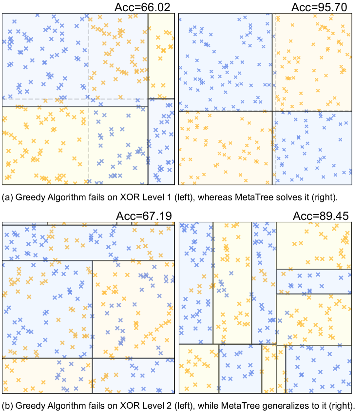
We generate a synthetic XOR dataset with the following algorithm: we first randomly sample 256 data points in the 2-dimensional bounding box $\{x|x\in[-1,1]^{2}\}$; then randomly generate the ground truth XOR splits inside the bounding box depending on the pre-specified level (for example, level 1 XOR has 3 splits, level 2 XOR has 15 splits, and the root node split can take place randomly $\in[-1,1]$ while the rest of the split is sampled randomly inside the dissected bounding boxes, see examples in Fig. 4) and assign the class labels according to the splits; at the final step, we add in label flipping noise and additional noisy feature dimensions consisted of uniform noise within $[-1,1]$.

4.2 Baselines

We use GOSDT (Lin et al., 2020) and CART (Breiman et al., 1984) as our baselines, as representative optimal and greedy decision tree algorithms. For GOSDT, we utilize the official implementation, using gradient-boosted decision trees for the initial label warm-up with the number of estimators equal to 128, a regularization factor of 1e-3. For CART, we use the implementation from sklearn (Pedregosa et al., 2011), with the splitting criterion set as Gini impurity.

4.3 Model configurations

We use LLaMA-2 (Touvron et al., 2023) as the base Transformer. For MetaTree, we set the number of layers as 12, the number of heads as 12, the embedding dimension as 768, MLP dimension as 3072.

We pretrain our model from scratch on the GOSDT dataset, and after training converges, we finetune it on the GOSDT+CART dataset. This curriculum improves performance compared to direct training on the GOSDT+CART dataset (as shown in Sec. A.3). Detailed training hyperparameters are shown in Sec. A.1.

5 Main results

In this section, we present MetaTree’s performance on real-world datasets previously unseen by the model (Fig. 1). We compare it with two established algorithms, GOSDT and CART, and find that it performs favorably, especially when ensembling across many trees. We focus on three questions: (1) Can MetaTree effectively generalize to real-world data it has not encountered before? (2) Is MetaTree capable of generating decision trees deeper than those it was trained on?, and (3) Can MetaTree be used in an LLM setting to accurately steer model outputs?

Generalizing to new datasets: Fig. 1A

To address the first question, we rigorously evaluate MetaTree across 91 datasets that were excluded from its training. For each dataset, we adopt the standard 70/30 split to create the train and test sets, then repeatedly sample from the train set and run the decision tree algorithms (MetaTree, GOSDT, or CART) to form tree ensembles with specified number of trees from {1, 5, 10, 20, 30, 40, 50, 60, 70, 80, 90, 100}. The majority prediction across trees is taken as the ensemble prediction and accuracy is averaged across all datasets. The entire evaluation process is replicated across 10 independent runs and the standard deviation is shown as error bars in the plot.

The result shows that MetaTree demonstrates a consistent and significant performance advantage over GOSDT and CART. Notably, all methods’ performance improved along with the increment of ensemble size, and plateaued when the number of trees reached 60. GOSDT outperforms CART when the number of trees is small; this corresponds well to GOSDT’s tendency to overfit on training data as it is designed to optimally solve for the train set. It also brings a higher variance in GOSDT’s generalization performance.

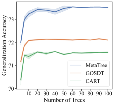
Generalizing to deeper trees: Fig. 1B

Going beyond MetaTree’s capability to generalize to new data, we now study whether MetaTree can generate deeper trees. To answer this question, we ask MetaTree to generate trees with depth 3, and compare its generalization performance with CART, similar to the aforementioned evaluation process.

The result is shown in Fig. 1B. It can be observed that MetaTree still consistently outperforms CART, with one exception when the number of trees is one, demonstrating MetaTree’s ability to generate beyond the tree depth it was trained on. We believe training MetaTree on deeper trees could further enhance this capability.

One reason why MetaTree can generalize to deeper trees is that it is designed to generate splitting decisions at each node, hence the generated tree is not dependent on the tree depth. Besides, the model has trained on depth 2 trees, i.e. the root node split and two children split, we believe our model might have learned to behave as an induction algorithm, thereby generating deeper trees with high quality.

Tree of prompts dataset: Fig. 1C

We evaluate MetaTree on the 13 Tree-of-prompt datasets, that consist of purely categorical features, with the input being LLM’s answer to a set of prompts (yes or no) and output being the classification label of the text. Fig. 1C again compares MetaTree to GOSDT and CART. MetaTree maintains a higher level of generalization accuracy across all tree counts when compared to GOSDT and CART. This trend is particularly noticeable as the number of trees increases, showing MetaTree’s robustness when the random effect of a single good/bad sample is diluted. GOSDT and CART show lower generalization accuracies, with GOSDT performing slightly better than CART, especially at lower tree counts.

This evaluation demonstrates MetaTree’s great performance on Tree-of-prompt datasets, highlighting its capability to process categorical features and produce differentiable trees for LLM-generated inputs and user-queried outputs.

Figure 4: Greedy algorithms such as CART cannot solve problems that require planning, such as Level 1&2 XOR. We show MetaTree can learn to solve Level 1 XOR and even generalize to solving Level 2 XOR, to a certain extent.

6 Analysis

After benchmarking the performance of MetaTree, we conduct an in-depth analysis of its behavior and splitting strategy. Our analysis of MetaTree begins in a controlled environment (Sec. 6.1), evaluating MetaTree’s performance in the presence of noise and feature interactions. We then take a closer look at MetaTree’s tendency between choosing a greedy split and an optimized split (Sec. 6.2), MetaTree’s internal decision-making process (Sec. 6.3), and MetaTree’s empirical bias-variance (Sec. 6.4).

6.1 Controlled setting: noisy XOR

We evaluate the MetaTree model in a controlled setting, on XOR datasets with level={1,2}, label flipping noise=$\{0\%,5\%,10\%,15\%,20\%,25\%\}$, and dataset size 10k for each XOR level/noise ratio configuration. To assess performance, we employ the relative error metric, defined as the gap between the achieved accuracy and the maximum possible accuracy achievable ($=100\%-\textrm{label noise rate}$). Note that we have only trained our model on 10k trees generated with XOR Level 1 and 15% label noise. This specific training scenario was chosen to evaluate the model’s robustness towards noise and adaptability to harder problems.

As indicated in Table 1, MetaTree demonstrates a remarkable capacity for noise resistance and generalization. Once MetaTree learned to solve the XOR Level 1 problem, it can withstand much stronger data noise (while MetaTree has only seen 15% noise), and generalize to significantly harder XOR Level 2 problems (while MetaTree has only trained on XOR Level 1).

Table 1: Relative error of MetaTree (trained on XOR Level 1 with 15% noise) on XOR datasets with level=$\{1,2\}$ and label flipping noise rate=$\{0\%,5\%,10\%,15\%,20\%,25\%\}$.

Noise	0%	5%	10%	15%	20%	25%
XOR L1	4.54	4.14	3.84	3.50	3.08	2.61
XOR L2	12.29	10.91	9.33	7.54	5.21	2.41

We further conduct a qualitative analysis, asking CART and MetaTree to generate decision trees for XOR Level 1&2 problems. The resulting trees, as depicted in Figure 4, offer insightful comparisons into the decision-making processes of both models under varying complexity levels.

(a) MetaTree tends to behave more like CART when CART generalizes better.

(b) MetaTree tends to behave more like GOSDT when GOSDT generalizes better.

(c) Generalization difference vs. MetaTree’s algorithmic preference.

Figure 5: We show that MetaTree learns to adapt its splitting strategy for better generalization. (a) and (b) demonstrate MetaTree’s tendency to select the more effective generalization strategy: opting for the greedy algorithm CART in (a) and the optimal algorithm GOSDT in (b). In (c), we show that MetaTree’s algorithmic preference is positively correlated with the algorithm’s generalization performance.

6.2 What splits are being made by MetaTree?

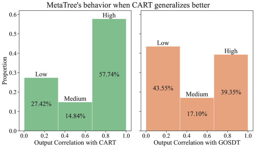
Our model is trained on mixed learning signals from GOSDT and CART, selected using generalization performance as the criterion. Our objective is to decipher whether MetaTree can strategically adapt its splitting approach between GOSDT and CART. To answer this question, we randomly take 100 samples (each of 256 data points) per dataset from the 91 left-out datasets and instruct MetaTree, GOSDT, and CART to generate splits for each sample. This approach ensures that all three algorithms are provided with the same data when making the splitting decision, allowing for a meaningful comparison.

We assess the similarity between the split generated by MetaTree and those produced by GOSDT and CART. To measure it, we calculate the correlation coefficient between the label assignments following the root node split. Additionally, we evaluate the generalization performance by examining the accuracy of the root node split on its respective test set. We exclude samples in cases where GOSDT and CART yield highly similar splits (correlation coefficient $>0.7$).

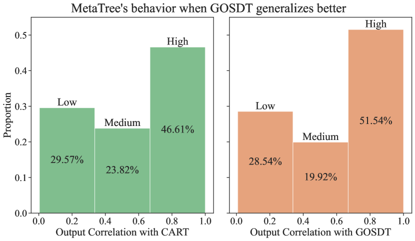
We plot the distribution of output correlation between MetaTree and CART/GOSDT in Fig. 5(a), for when CART is the better generalizing algorithm among the two. Similarly, we plot the output correlation between MetaTree and CART/GOSDT in Fig. 5(b) for when GOSDT is better generalizing. We divide the output correlation values into three categories (low, medium, and high correlation), and it can be observed that MetaTree tends to favor the algorithm that exhibits better generalization performance.

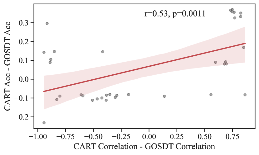
Furthermore, we visualize the relationship between the correlation difference (CART correlation minus GOSDT correlation) and the generalization performance difference (CART’s test accuracy minus GOSDT’s test accuracy) in Fig. 5(c), noting that we exclude samples with marginal performance differences (generalization accuracy difference $\leq$ 0.08). A medium correlation (Pearson correlation = 0.53, p-value = 0.0011) is observed, suggesting a tendency in MetaTree’s splitting strategy to align with generalization performance.

6.3 Probing MetaTree’s decision-making process

Our study is partially inspired by the logit-lens behavior analysis on GPT-2 (Hanna et al., 2023). Their findings suggest that GPT-2 often forms an initial guess about the next token in its middle layers, with subsequent layers refining this guess for the final generation distribution. Building on this concept, we aim to investigate whether a similar guessing-refining pattern exists in our model and explore the feasibility of implementing an early exiting strategy as outlined in Zhou et al. (2020).

(a) Logit-lens probing of MetaTree on an XOR Level 1 problem.

(b) The output correlation analysis between the final split and each layer’s splits of MetaTree across 91 left-out datasets.

Figure 6: Probing the internal decision process of MetaTree.

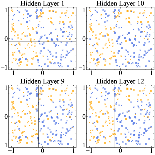
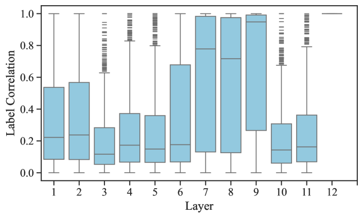
To this end, we analyze the decision-making process of our model at each Transformer layer. We can scrutinize how the model’s decisions evolve by feeding the intermediate representation from each layer into the output module. One qualitative example is shown in Fig. 6(a), where we ask MetaTree to generate the root node split on an XOR Level 1 problem. We can observe that the model gets a reasonable split right after the first layer. At layer 9, the model reaches the split that is close to its final output, and layer 10’s output is an alternative revision with a close to ground truth split (the ground truth can be a vertical or horizontal split).

We proceed with a quantitative analysis to investigate the correlation between the model’s final split and the splits occurring in its intermediate layers. We take samples from the 91 left-out datasets following the same procedure as detailed in Sec. 6.2, and we ask MetaTree to generate splits on them. The correlation between splits is determined by the correlation coefficient between the label assignments after applying the splits. This metric essentially measures how closely aligned the splits are in dissecting input regions.

The results of our quantitative analysis are presented in Fig. 6(b). Notably, the correlation shows a gradual increase from layer 1 to 8, nearly reaching 1 at layer 9. However, it then drops significantly to approximately 0.2 at layers 10 and 11. This pattern suggests that the model consistently improves its ability to make accurate predictions in the initial 1 to 9 layers, while layers 10 and 11 may introduce some divergence or revision in its decision-making process.

This finding provides valuable insights into the internal decision-making process of MetaTree. It raises the possibility of considering early exit strategies at intermediate layers, particularly around layer 9, to enhance overall efficiency.

6.4 Bias-variance analysis

Finally, we conduct a comprehensive bias-variance analysis to evaluate MetaTree, along with GOSDT and CART, on the 91 left-out datasets. This analysis shows how each algorithm navigates the trade-off between bias (the error due to insufficient learning power of the algorithm or incorrect model assumptions) and variance (the error due to sensitivity to small fluctuations in the training set). We use the empirical bias and variance as the measures in our evaluation; we perform 100 repetitions (N=100) for each dataset, therefore we have 100 decision tree models per algorithm per dataset. The empirical bias of an algorithm is calculated as the $\ell_{2}$ difference between its produced models’ average output and the ground truth labels, whereas the empirical variance is calculated as the mean $\ell_{2}$ difference between its produced models’ average output and each model’s output.

Figure 7: Empirical Bias-Variance comparison for MetaTree, GOSDT, and CART on 91 left-out datasets with 100 repetitions. MetaTree has significantly lower variance and slightly smaller bias as compared to GOSDT and CART.

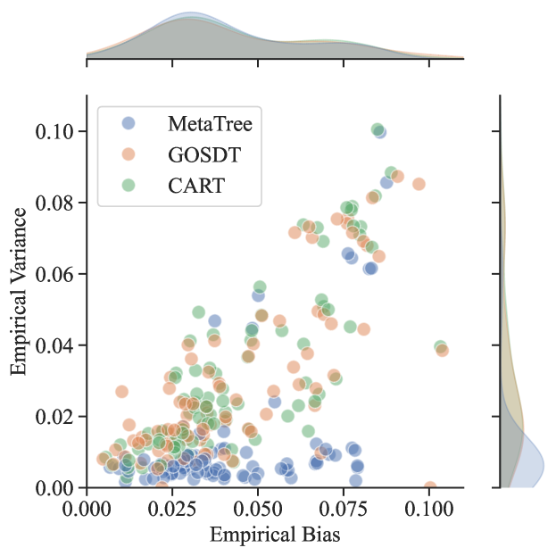
The result is presented in Fig. 7. Each point in the plot corresponds to the bias-variance coordinates derived from the performance of one algorithm on a single dataset. The x-axis represents empirical bias, indicating the algorithm’s average error from the true function, while the y-axis corresponds to empirical variance, reflecting the sensitivity of the algorithm to different training sets. It can be observed that MetaTree demonstrates lower empirical variance, suggesting its robustness in diverse data distribution scenarios.

7 Discussion

Limitations and future directions

MetaTree is constrained by the inherent architectural limitations of Transformers. Specifically, the maximum number of data points and features that MetaTree can process is bounded by the Transformer model’s max sequence length (refer to Table 2 for detailed specifications). However, these constraints can be alleviated by training a larger model. Transformers’ capacity for handling long sequences is constantly improving, with state-of-the-art LLMs (OpenAI, 2023) now able to take in sequences with up to 128k tokens. While MetaTree remains limited to small datasets, this work shows an important first step in learning to adaptively produce machine-learning models, and we leave training a large-scale LLM for future work.

Conclusion

We introduce MetaTree, a novel transformer-based decision tree algorithm. It diverges from traditional heuristic-based or optimization-based decision tree algorithms, leveraging the learning capabilities of transformers to generate strong decision tree models. MetaTree is trained using data from classical decision tree algorithms and exhibits a unique ability to adapt its strategy to the dataset context, thus achieving superior generalization performance. The model demonstrates its efficacy on unseen real-world datasets and can generalize to generate deeper trees. We conducted a thorough analysis of MetaTree’s behavior, internal decision-making process, and bias-variance characteristics. This work showcases the potential of deep learning models in algorithm generation, broadening their scope beyond predicting labels and into the realm of automated model creation. Its ability to learn from and improve upon established algorithms opens new avenues for research and application in the field of machine learning.

Broader impacts

This paper presents work whose goal is to advance the field of Machine Learning. There are many potential societal consequences of our work, none which we feel must be specifically highlighted here.

Appendix A Appendix

A.1 Model Hyperparameters

Table 2: Hyperparameters for MetaTree training.

Hyperparameter	Value
Number of Hidden Layers	12
Number of Attention Heads	12
Hidden Size	768
Learning Rate	5e-5
Learning Rate Schedule	Linear Decay
Optimizer	AdamW
$\beta_{1}$	0.9
$\beta_{2}$	0.999
Training dtype	fp16
Number of Features	10
Number of Classes	10
Block Size	256
Tree Depth	2
$\sigma$	5e-2
Number of Warmup Steps	1000
Number of Training Steps	2,000,000
Steps in Phase 1 (GOSDT)	1,000,000
Steps in Phase 2 (GOSDT+CART)	1,000,000
Batch Size	128

A.2 Ablation Study: Gaussian Smoothing Loss

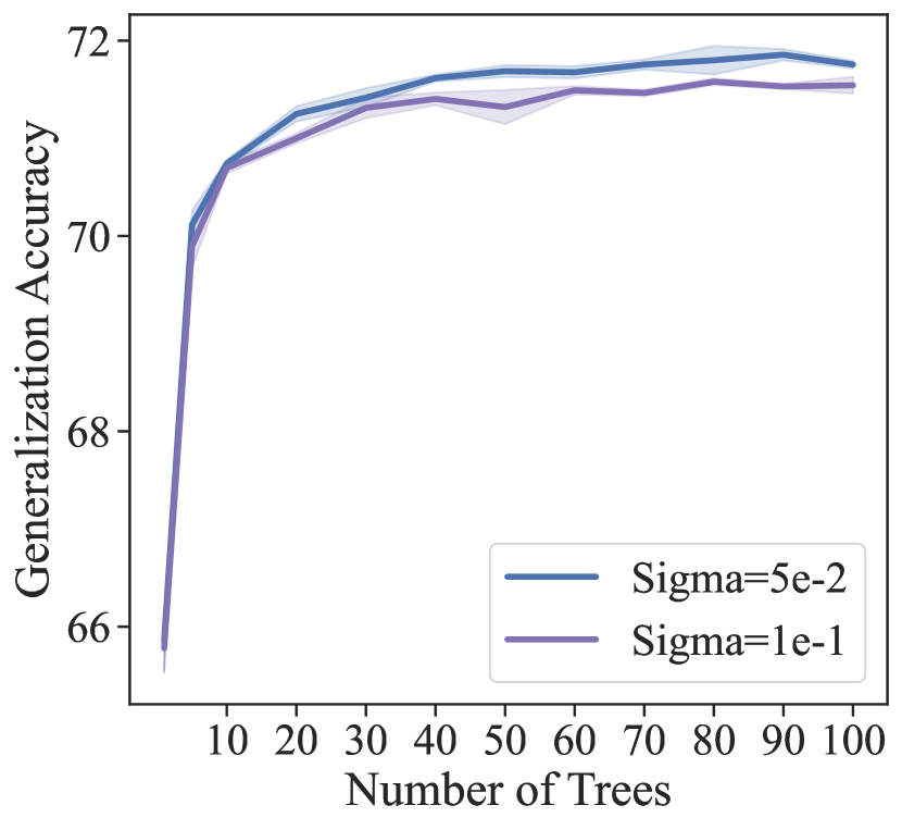
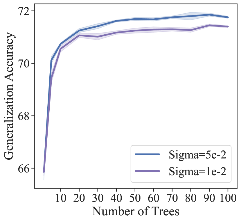
We conduct an ablation study on the radius of the Gaussian smoothing loss ($\sigma$). It controls how much noise and signal the model receives during training. When $\sigma$ is too large, every split may seem like a target split, but when $\sigma$ is too small, the model may fail to learn from some equally good splits.

Following the evaluation pipeline as described in Sec. 5, we conduct our ablation study comparing our model trained using $\sigma$=5e-1 with models trained with a larger $\sigma$=1e-1 and a smaller $\sigma$=1e-2, on 91 left-out datasets and compute their average test accuracy for number of trees from {1, 5, 10, 20, 30, 40, 50, 60, 70, 80, 90, 100}.

As shown in Fig. 8, the smoothing radius does have an impact on the trained model, and choosing an appropriate radius is essential to training an effective model.

(a) Training with a larger $\sigma$=1e-1.

(b) Training with a smaller $\sigma$=1e-2.

Figure 8: Average generalization accuracy for models trained with different Gaussian Smoothing radius.

A.3 Ablation Study: Training Curriculum

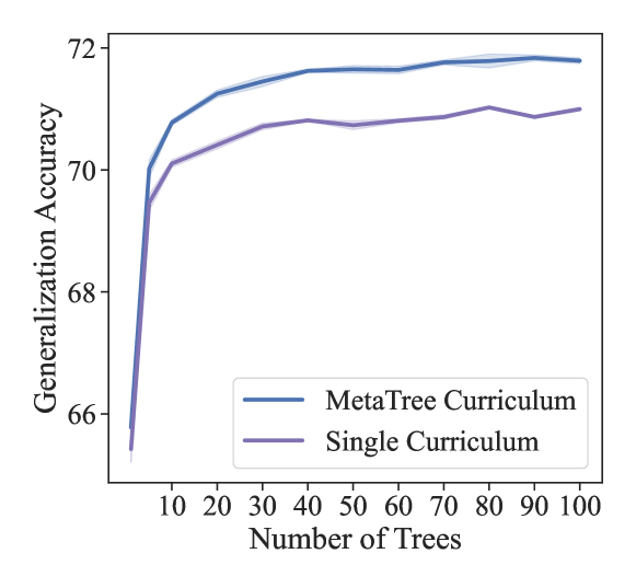
We devise a two-phase learning curriculum for MetaTree’s training, as described in Sec. 3.1. Here we conduct an ablation study comparing our curriculum with a curriculum that only uses the GOSDT+CART dataset with otherwise same configurations.

The evaluation process is the same as the one used in Sec. 5, we compute their average test accuracy on 91 left-out datasets and for the number of trees from {1, 5, 10, 20, 30, 40, 50, 60, 70, 80, 90, 100}.

As shown in Fig. 9, the learning curriculum has a significant impact on the model at the end of training.

Figure 9: Average generalization accuracy for two different learning curricula. MetaTree’s learning curriculum involves a first-phase training on GOSDT trees only, and a second-phase training on GOSDT+CART trees. The other curriculum is trained directly from GOSDT+CART datasets.

Figure 10: Average generalization accuracy for models trained with or without positional bias.

A.4 Ablation Study: Positional Bias

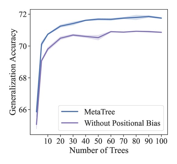
As introduced in Fig. 3, MetaTree uses two positional bias $b_{1},b_{2}$ at the input layer to anchor the row and column positions. We apply sequential and dimensional shuffling during training to make the model learn the positional invariance.

Alternatively, we can have a design that provides zero positional information to the model and becomes naturally invariant to input permutations. However, this design may have difficulties identifying the split, as the information will be mixed altogether over the Transformer layers.

We train a model with such a design, keeping all other training configurations the same, and compare its performance on the 91 left-out datasets using their average test accuracy for the number of trees from {1, 5, 10, 20, 30, 40, 50, 60, 70, 80, 90, 100}.

As shown in Fig. 10, having such positional bias is empirically beneficial compared to a design that provides no positional information to the model.

A.5 Memory Usage of GOSDT

We conduct an analysis to show the memory usage difference between CART — an efficient algorithm with greedy heuristics and GOSDT — a mathematically guaranteed optimized algorithm.

The frequent out-of-memory or out-of-time issue is the main reason for us to exclude GOSDT in the Depth 3 study.

Table 3: We show the memory usage of CART and GOSDT when fitting decision trees with depth 2 & 3, using the memory profiler tool (Pedregosa & Gervais, 2021). GOSDT takes a significant amount of memory since it is solving for the full decision tree solution on the data. *We report successfully terminated runs’ stats, the experiments are conducted on a workstation with 125G memories and 128 cores.

		CART	GOSDT
Depth=2	Mean Memory	0.82 MB	146.82 MB*
	Max Memory	1.41 MB	228.98 MB*
	Fail Rate	0%	1.1%
Depth=3	Mean Memory	0.79 MB	15,615.69 MB*
	Max Memory	1.34 MB	87,721.02 MB*
	Fail Rate	0%	86.81%

A.6 Datasets

Table 4: List of 91 datasets used in MetaTree’s evaluation.

Dataset	Entries	Dim.	Class
mfeat fourier	2000	76	10
mfeat zernike	2000	47	10
mfeat morphological	2000	6	10
mfeat karhunen	2000	64	10
page blocks	5473	10	5
optdigits	5620	64	10
pendigits	10992	16	10
waveform 5000	5000	40	3
Hyperplane 10 1E 3	1000000	10	2
Hyperplane 10 1E 4	1000000	10	2
pokerhand	829201	5	10
RandomRBF 0 0	1000000	10	5
RandomRBF 10 1E 3	1000000	10	5
RandomRBF 50 1E 3	1000000	10	5
RandomRBF 10 1E 4	1000000	10	5
RandomRBF 50 1E 4	1000000	10	5
SEA 50	1000000	3	2
SEA 50000	1000000	3	2
satimage	6430	36	6
BNG labor	1000000	8	2
BNG breast w	39366	9	2
BNG mfeat karhunen	1000000	64	10
BNG bridges version1	1000000	3	6
BNG mfeat zernike	1000000	47	10
BNG cmc	55296	2	3
BNG colic ORIG	1000000	7	2
BNG colic	1000000	7	2
BNG credit a	1000000	6	2
BNG page blocks	295245	10	5
BNG credit g	1000000	7	2
BNG pendigits	1000000	16	10
BNG cylinder bands	1000000	18	2
BNG dermatology	1000000	1	6
BNG sonar	1000000	60	2
BNG glass	137781	9	7
BNG heart c	1000000	6	5
BNG heart statlog	1000000	13	2
BNG vehicle	1000000	18	4
BNG hepatitis	1000000	6	2
BNG waveform 5000	1000000	40	3
BNG zoo	1000000	1	7
vehicle sensIT	98528	100	2
UNIX user data	9100	1	9
fri c3 1000 25	1000	25	2
rmftsa sleepdata	1024	2	4
JapaneseVowels	9961	14	9
fri c4 1000 100	1000	100	2
abalone	4177	7	2
fri c4 1000 25	1000	25	2
bank8FM	8192	8	2
analcatdata supreme	4052	7	2
ailerons	13750	40	2
cpu small	8192	12	2
space ga	3107	6	2
fri c1 1000 5	1000	5	2
puma32H	8192	32	2
fri c3 1000 10	1000	10	2
cpu act	8192	21	2
fri c4 1000 10	1000	10	2
quake	2178	3	2
fri c4 1000 50	1000	50	2
fri c0 1000 5	1000	5	2
delta ailerons	7129	5	2
fri c3 1000 50	1000	50	2
kin8nm	8192	8	2
fri c3 1000 5	1000	5	2
puma8NH	8192	8	2
delta elevators	9517	6	2
houses	20640	8	2
bank32nh	8192	32	2
fri c1 1000 50	1000	50	2
house 8L	22784	8	2
fri c0 1000 10	1000	10	2
elevators	16599	18	2
wind	6574	14	2
fri c0 1000 25	1000	25	2
fri c2 1000 50	1000	50	2
pollen	3848	5	2
mv	40768	7	2
fried	40768	10	2
fri c2 1000 25	1000	25	2
fri c0 1000 50	1000	50	2
fri c1 1000 10	1000	10	2
fri c2 1000 5	1000	5	2
fri c2 1000 10	1000	10	2
fri c1 1000 25	1000	25	2
visualizing soil	8641	3	2
socmob	1156	1	2
mozilla4	15545	5	2
pc3	1563	37	2
pc1	1109	21	2

References

- Agarwal et al. (2022) Agarwal, A., Tan, Y. S., Ronen, O., Singh, C., and Yu, B. Hierarchical shrinkage: improving the accuracy and interpretability of tree-based methods. arXiv:2202.00858 [cs, stat], 2 2022. URL http://arxiv.org/abs/2202.00858. arXiv: 2202.00858.
- Bertsimas & Dunn (2017) Bertsimas, D. and Dunn, J. Optimal classification trees. Machine Learning, 106(7):1039–1082, 2017.
- Betker et al. (2023) Betker, J., Goh, G., Jing, L., Brooks, T., Wang, J., Li, L., Ouyang, L., Zhuang, J., Lee, J., Guo, Y., et al. Improving image generation with better captions. Computer Science. https://cdn. openai. com/papers/dall-e-3. pdf, 2:3, 2023.
- Breiman (2001) Breiman, L. Random forests. Machine Learning, 45(1):5–32, 10 2001. ISSN 1573-0565. doi: 10.1023/A:1010933404324.
- Breiman et al. (1984) Breiman, L., Friedman, J. H., Olshen, R. A., and Stone, C. J. Classification and Regression Trees. Wadsworth and Brooks, Monterey, CA, 1984. URL https://www.routledge.com/Classification-and-Regression-Trees/Breiman-Friedman-Stone-Olshen/p/book/9780412048418.
- Carreira-Perpinán & Tavallali (2018) Carreira-Perpinán, M. A. and Tavallali, P. Alternating optimization of decision trees, with application to learning sparse oblique trees. Advances in neural information processing systems, 31, 2018.
- Chipman et al. (2010) Chipman, H. A., George, E. I., and McCulloch, R. E. Bart: Bayesian additive regression trees. The Annals of Applied Statistics, 4(1):266–298, 2010.
- Dziri et al. (2023) Dziri, N., Lu, X., Sclar, M., Li, X. L., Jian, L., Lin, B. Y., West, P., Bhagavatula, C., Bras, R. L., Hwang, J. D., et al. Faith and fate: Limits of transformers on compositionality. arXiv preprint arXiv:2305.18654, 2023.
- Fawzi et al. (2022) Fawzi, A., Balog, M., Huang, A., Hubert, T., Romera-Paredes, B., Barekatain, M., Novikov, A., R Ruiz, F. J., Schrittwieser, J., Swirszcz, G., et al. Discovering faster matrix multiplication algorithms with reinforcement learning. Nature, 610(7930):47–53, 2022.
- Feuer et al. (2023) Feuer, B., Hegde, C., and Cohen, N. Scaling tabpfn: Sketching and feature selection for tabular prior-data fitted networks. arXiv preprint arXiv:2311.10609, 2023.
- Freund et al. (1996) Freund, Y., Schapire, R. E., et al. Experiments with a new boosting algorithm. In icml, volume 96, pp. 148–156. Citeseer, 1996.
- Garg et al. (2022) Garg, S., Tsipras, D., Liang, P. S., and Valiant, G. What can transformers learn in-context? a case study of simple function classes. Advances in Neural Information Processing Systems, 35:30583–30598, 2022.
- Gorishniy et al. (2023) Gorishniy, Y., Rubachev, I., Kartashev, N., Shlenskii, D., Kotelnikov, A., and Babenko, A. Tabr: Unlocking the power of retrieval-augmented tabular deep learning. arXiv preprint arXiv:2307.14338, 2023.
- Grinsztajn et al. (2022) Grinsztajn, L., Oyallon, E., and Varoquaux, G. Why do tree-based models still outperform deep learning on typical tabular data? Advances in Neural Information Processing Systems, 35:507–520, 2022.
- Hanna et al. (2023) Hanna, M., Liu, O., and Variengien, A. How does gpt-2 compute greater-than?: Interpreting mathematical abilities in a pre-trained language model. arXiv preprint arXiv:2305.00586, 2023.
- Hegselmann et al. (2023) Hegselmann, S., Buendia, A., Lang, H., Agrawal, M., Jiang, X., and Sontag, D. Tabllm: Few-shot classification of tabular data with large language models. In International Conference on Artificial Intelligence and Statistics, pp. 5549–5581. PMLR, 2023.
- Hollmann et al. (2022) Hollmann, N., Müller, S., Eggensperger, K., and Hutter, F. Tabpfn: A transformer that solves small tabular classification problems in a second. arXiv preprint arXiv:2207.01848, 2022.
- Hospedales et al. (2021) Hospedales, T., Antoniou, A., Micaelli, P., and Storkey, A. Meta-learning in neural networks: A survey. IEEE transactions on pattern analysis and machine intelligence, 44(9):5149–5169, 2021.
- Hu et al. (2019) Hu, X., Rudin, C., and Seltzer, M. Optimal sparse decision trees. Advances in Neural Information Processing Systems (NeurIPS), 2019.
- Kornblith et al. (2022) Kornblith, A. E., Singh, C., Devlin, G., Addo, N., Streck, C. J., Holmes, J. F., Kuppermann, N., Grupp-Phelan, J., Fineman, J., Butte, A. J., and Yu, B. Predictability and stability testing to assess clinical decision instrument performance for children after blunt torso trauma. medRxiv, 2022. doi: 10.1101/2022.03.08.22270944. URL https://www.medrxiv.org/content/early/2022/03/08/2022.03.08.22270944.
- Laurent & Rivest (1976) Laurent, H. and Rivest, R. L. Constructing optimal binary decision trees is np-complete. Information processing letters, 5(1):15–17, 1976.
- Lin et al. (2020) Lin, J., Zhong, C., Hu, D., Rudin, C., and Seltzer, M. Generalized and scalable optimal sparse decision trees. In International Conference on Machine Learning, pp. 6150–6160. PMLR, 2020.
- Manikandan et al. (2023) Manikandan, H., Jiang, Y., and Kolter, J. Z. Language models are weak learners. arXiv preprint arXiv:2306.14101, 2023.
- Mankowitz et al. (2023) Mankowitz, D. J., Michi, A., Zhernov, A., Gelmi, M., Selvi, M., Paduraru, C., Leurent, E., Iqbal, S., Lespiau, J.-B., Ahern, A., et al. Faster sorting algorithms discovered using deep reinforcement learning. Nature, 618(7964):257–263, 2023.
- Morris et al. (2023) Morris, J. X., Singh, C., Rush, A. M., Gao, J., and Deng, Y. Tree prompting: efficient task adaptation without fine-tuning. arXiv preprint arXiv:2310.14034, 2023.
- Nichol et al. (2018) Nichol, A., Achiam, J., and Schulman, J. On first-order meta-learning algorithms. arXiv preprint arXiv:1803.02999, 2018.
- Onishi et al. (2023) Onishi, S., Oono, K., and Hayashi, K. Tabret: Pre-training transformer-based tabular models for unseen columns. arXiv preprint arXiv:2303.15747, 2023.
- OpenAI (2023) OpenAI. Gpt-4 technical report, 2023.
- Pedregosa & Gervais (2021) Pedregosa, F. and Gervais, P. memory-profiler: A module for monitoring memory usage of a python program. https://pypi.org/project/memory-profiler/, 2021.
- Pedregosa et al. (2011) Pedregosa, F., Varoquaux, G., Gramfort, A., Michel, V., Thirion, B., Grisel, O., Blondel, M., Prettenhofer, P., Weiss, R., Dubourg, V., Vanderplas, J., Passos, A., Cournapeau, D., Brucher, M., Perrot, M., and Duchesnay, E. Scikit-learn: Machine learning in Python. Journal of Machine Learning Research, 12:2825–2830, 2011.
- Quinlan (1986) Quinlan, J. R. Induction of decision trees. Machine learning, 1(1):81–106, 1986.
- Quinlan (2014) Quinlan, J. R. C4. 5: programs for machine learning. Elsevier, 2014.
- Romano et al. (2021) Romano, J. D., Le, T. T., La Cava, W., Gregg, J. T., Goldberg, D. J., Chakraborty, P., Ray, N. L., Himmelstein, D., Fu, W., and Moore, J. H. Pmlb v1.0: an open source dataset collection for benchmarking machine learning methods. arXiv preprint arXiv:2012.00058v2, 2021.
- Romera-Paredes et al. (2023) Romera-Paredes, B., Barekatain, M., Novikov, A., Balog, M., Kumar, M. P., Dupont, E., Ruiz, F. J., Ellenberg, J. S., Wang, P., Fawzi, O., et al. Mathematical discoveries from program search with large language models. Nature, pp. 1–3, 2023.
- Singh et al. (2023) Singh, C., Askari, A., Caruana, R., and Gao, J. Augmenting interpretable models with large language models during training. Nature Communications, 14(1):7913, 2023.
- Tan et al. (2022) Tan, Y. S., Singh, C., Nasseri, K., Agarwal, A., and Yu, B. Fast interpretable greedy-tree sums (figs). arXiv:2201.11931 [cs, stat], 1 2022. URL http://arxiv.org/abs/2201.11931. arXiv: 2201.11931.
- Touvron et al. (2023) Touvron, H., Martin, L., Stone, K., Albert, P., Almahairi, A., Babaei, Y., Bashlykov, N., Batra, S., Bhargava, P., Bhosale, S., et al. Llama 2: Open foundation and fine-tuned chat models. arXiv preprint arXiv:2307.09288, 2023.
- Vanschoren et al. (2013) Vanschoren, J., van Rijn, J. N., Bischl, B., and Torgo, L. Openml: networked science in machine learning. SIGKDD Explorations, 15(2):49–60, 2013. doi: 10.1145/2641190.2641198. URL http://doi.acm.org/10.1145/2641190.264119.
- Vaswani et al. (2017) Vaswani, A., Shazeer, N., Parmar, N., Uszkoreit, J., Jones, L., Gomez, A. N., Kaiser, Ł., and Polosukhin, I. Attention is all you need. Advances in neural information processing systems, 30, 2017.
- Vilalta & Drissi (2002) Vilalta, R. and Drissi, Y. A perspective view and survey of meta-learning. Artificial intelligence review, 18:77–95, 2002.
- Yadlowsky et al. (2023) Yadlowsky, S., Doshi, L., and Tripuraneni, N. Can transformer models generalize via in-context learning beyond pretraining data? In NeurIPS 2023 Workshop on Distribution Shifts: New Frontiers with Foundation Models, 2023.
- Yao et al. (2023) Yao, S., Yu, D., Zhao, J., Shafran, I., Griffiths, T. L., Cao, Y., and Narasimhan, K. Tree of thoughts: Deliberate problem solving with large language models, 2023.
- Zhou et al. (2023) Zhou, H., Bradley, A., Littwin, E., Razin, N., Saremi, O., Susskind, J., Bengio, S., and Nakkiran, P. What algorithms can transformers learn? a study in length generalization. arXiv preprint arXiv:2310.16028, 2023.
- Zhou et al. (2020) Zhou, W., Xu, C., Ge, T., McAuley, J., Xu, K., and Wei, F. Bert loses patience: Fast and robust inference with early exit. Advances in Neural Information Processing Systems, 33:18330–18341, 2020.
- Zhu et al. (2023) Zhu, B., Shi, X., Erickson, N., Li, M., Karypis, G., and Shoaran, M. Xtab: Cross-table pretraining for tabular transformers. arXiv preprint arXiv:2305.06090, 2023.