Pre-training of Lightweight Vision Transformers on Small Datasets with Minimally Scaled Images

Abstract

Can a lightweight Vision Transformer (ViT) match or exceed the performance of Convolutional Neural Networks (CNNs) like ResNet on small datasets with small image resolutions? This report demonstrates that a pure ViT can indeed achieve superior performance through pre-training, using a masked auto-encoder technique with minimal image scaling. Our experiments on the CIFAR-10 and CIFAR-100 datasets involved ViT models with fewer than 3.65 million parameters and a multiply-accumulate (MAC) count below 0.27G, qualifying them as ’lightweight’ models. Unlike previous approaches, our method attains state-of-the-art performance among similar lightweight transformer-based architectures without significantly scaling up images from CIFAR-10 and CIFAR-100. This achievement underscores the efficiency of our model, not only in handling small datasets but also in effectively processing images close to their original scale.

1 Introduction

In the rapidly evolving field of computer vision, the quest for more efficient and effective models remains a central research focus. Traditionally, Convolutional Neural Networks (CNNs) [1, 2, 3] have dominated this domain, especially in tasks involving small datasets. However, the emergence of Vision Transformers (ViTs) [4] has introduced a paradigm shift, challenging the supremacy of CNNs in certain applications. Despite their success in large-scale datasets, ViTs have struggled to match the performance of CNNs in smaller data scenarios due to their lack of inherent inductive biases [4], as a result, CNNs are still the preferred architectures for smaller datasets [5].

Addressing this gap, our study explores the potential of ViTs in contexts where data availability is limited. The central hypothesis of our research is that a lightweight ViT can perform as well as, or even better than, its CNN counterparts like ResNet [3] on small datasets. To investigate this, we have employed a pre-training strategy using Masked Auto-Encoder (MAE) [6] to enhance the capability of ViTs to learn from smaller datasets effectively.

In this report, we detail a series of experiments conducted to test the effectiveness of lightweight ViTs when pre-trained with a MAE on small datasets. We present the adaptations made to the conventional ViT and MAE structure to improve its suitability for smaller datasets and document the implementation of our pre-training regimen. Our results indicate that with these modifications, ViTs can indeed reach or exceed the performance benchmarks set by CNNs on smaller datasets.

2 Method

In our implementation of the Masked Auto-Encoder (MAE), we largely follow the process outlined in the original MAE paper [6]. We start by dividing each image into non-overlapping patches, similar to the ViT [4]. From these patches, a subset is randomly selected without replacement, following a uniform distribution. These selected patches are known as the unmasked patches and fed into the Encoder. The remaining patches are the masked patches, which are not directly used in the encoding step. We adopt the masking ratio of 0.75, as recommended by the original MAE paper, so that 75% of the total patches are masked and not included in the initial input to the encoder. See Figure 1.

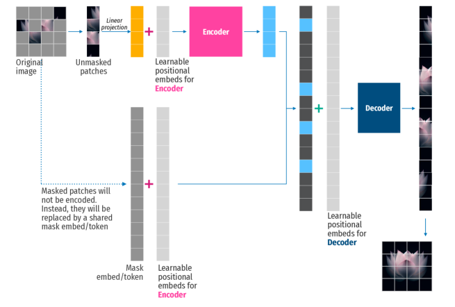
Figure 1: Modified MAE: Implementation using separate learnable positional embeddings for Encoder and Decoder. The Encoder and the Decoder in this figure only consist of transformer layers, a layer of layerNorm and a linear projection layer.

2.1 MAE Encoder

Our encoder adopts the structure of a ViT [4], but it operates only on the visible, unmasked patches of an image. In line with standard ViT models, our encoder first applies a linear projection to embed these patches, enhancing them with positional information, followed by a series of transformer layers [7] and a linear projection layer. Layer normalization [8] is applied before the input to the linear projection layer. See Figure 2.

However, diverging from both the original ViT and MAE implementations [6], our encoder utilizes learnable positional embeddings instead of the traditional sinusoidal positional embeddings. Given that our masking ratio is set to 0.75, the encoder is essentially processing only a quarter (25%) of the total patches in an image. The masked patches, which comprise the majority of the image data, are excluded from this phase of processing.

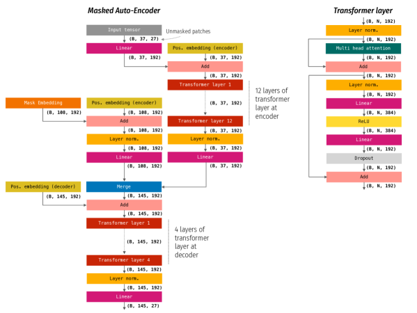
Figure 2: The architecture of our MAE. ’B’ stands for batch size, ’N’ for number of embeddings

2.2 MAE Decoder

The MAE decoder in our model is responsible for reconstructing the image from a comprehensive set of embeddings, which includes both the encoded visible patches and mask embeddings. These mask embeddings [9] are shared, learnable vectors that signify the presence of each missing patch that the model aims to predict. Unlike the original MAE implementation [6], we incorporate separate learnable positional embeddings at the decoder’s input, ensuring precise spatial awareness in the reconstruction phase.

Structurally, the decoder consists of a series of transformer layers, a layer normalization and a linear projection layer, similar to the encoder. However, the decoder’s architecture is not constrained by the design of the encoder. This independence allows for greater flexibility in its configuration. We can, for instance, opt for a different embedding size or a varying number of transformer layers in the decoder compared to the encoder.

The use of the MAE decoder is exclusive to the pre-training phase, where its primary function is to reconstruct the original image from the partial input provided by the encoder. This specialized role allows us to tailor the decoder’s design specifically for optimal reconstruction performance, independent of the encoder’s configuration.

2.3 Reconstruction Output

In our MAE model, the reconstruction of the input image is achieved by predicting the pixel values for each masked patch, aligning with the approach used in the original MAE. The decoder’s output for each patch is a vector that corresponds to the pixel values of the patch. This output undergoes a linear projection in the final layer of the decoder, with the number of output neurons matching the number of pixel values in a patch. We then reshape this output to form the reconstructed image.

A key aspect of our implementation is the application of the loss function. The original MAE uses the mean squared error (MSE) to measure the difference between the reconstructed and original images in pixel space. However, unlike the original MAE where the loss is calculated solely on the masked patches (akin to the strategy used in BERT [9]), our approach modifies this calculation. We compute the total loss as a sum of the loss on masked patches and an additional, discounted loss on unmasked patches:

$$\mathrm{Loss}=\mathrm{MSE}_{\mathrm{masked\_patches}}+\alpha\cdot\mathrm{MSE}_{\mathrm{unmasked\_patches}}$$ (1)

$\alpha$ denotes the discounting factor. This variation addresses a specific issue observed in the original implementation, where no loss was computed on visible patches, leading to a lower quality in model output for these patches. By incorporating a discounted loss on unmasked patches, we not only observe a reduction in the total loss (compared to calculating it only on masked patches) but also a significant improvement in the quality of the reconstructed visible patches.

3 Experimental Setup

In our experimental setup, we conduct self-supervised pre-training on the CIFAR10 [10] and CIFAR100 [10] training datasets separately. Following this pre-training phase, each model is fine-tuned for classification tasks on the respective CIFAR10 and CIFAR100 datasets. We use the same random seed for all of our experiments.

A notable aspect of our implementation is the adjustment of the image input size to 36 x 36, slightly larger than the original 32 x 32 dimension of these datasets. This size change results in each image being divided into 144 patches, given our chosen patch size of 3 x 3.

We add an auxiliary dummy patch to each image during both the pre-training and fine-tuning phases. This dummy patch, which contains zero values for all elements, is appended as the 145th patch. The encoded embedding of this auxiliary patch is utilized for classification purposes. Consequently, this adjustment necessitates a total of 145 positional embeddings for both the encoder and decoder in our model, accommodating the extra dummy patch.

3.1 Encoder and Decoder design

Our Masked Auto-Encoder employs encoders and decoders both with an embedding size of 192, and each utilizes 3 heads. The encoder is composed of 12 transformer layers, while the decoder features 4 transformer layers.

Within each transformer layer (see Figure 2), we opt for the ReLU [11] activation function instead of the GELU [12], which is used in the original Vision Transformer (ViT) [4]. Each layer includes a sequence of two linear layers: the first expanding the output to twice (rather than 4 times) the embedding size, followed by ReLU activation, and the second linear layer reducing it back to the embedding size. We apply dropout [13] with a rate of 0.1 to the output of these layers . All linear layers within the transformer layers are included with bias. However, we exclude bias from other linear projection layers in both the encoder and decoder.

For initializing weights and biases across all layer types, we rely on the default methods provided by Pytorch. The same applies to our approach to layer normalization [8], where we use Pytorch’s default setup.

3.2 Pre-training

Our pre-training process is arranged for 4000 epochs, employing the AdamW optimizer [14] with a weight decay set at 0.05. The initial 400 epochs are designated for warm-up [15]. We follow this with a cosine decay schedule [16] for the learning rate. The batch size during training is 1408, and we adhere to the linear learning rate scaling rule with a base learning rate of $1.5e-4$ [15, 6]:

$$\mathrm{lr}=\mathrm{base\_lr}\times\mathrm{batch\_size}/256$$ (2)

In terms of data augmentation, we randomly flip the input images horizontally with a 50% probability. Additionally, we utilize random resized cropping, with a scale range from 0.6 to 1. For color normalization, we apply a mean of 0.5 and a standard deviation of 0.5 to each color channel. The discounting factor ($\alpha$) in Eq. 2 is set to 0.1. See Table 1 for recipe.

Table 1: Parameters and Configuration for Pre-Training

Configuration	Value
Optimizer	AdamW
Weight decay	0.05
Base learning rate	$1.5e-4$
Learning rate schedule	Cosine decay
Total epochs	4000
Warm-up epochs	400
Batch size	1408
Horizontal flipping	$p=0.5$
Random resized cropping	$[0.6,1]$
Color normalization	$\mathrm{mean}=0.5,\mathrm{std}=0.5$
Discounting factor ($\alpha$)	0.1

3.3 Fine-tuning

For fine-tuning, we use the pre-trained MAE encoder for classification tasks on CIFAR10 and CIFAR100 datasets. The fine-tuning architecture comprises the MAE encoder and an additional linear layer. The input to this linear layer is the last embedding from the encoder, which corresponds to the dummy patch. We fine-tune for 300 epochs, with the initial 20 epochs serving as a warm-up period [15]. This is followed by a cosine decay learning rate schedule [16]. The optimizer used is AdamW [14] with a weight decay of 0.05, and the batch size is set at 768. We adhere to a linear learning rate scaling rule (Eq. 1), starting with a base learning rate of $1e-3$ and applying a layer-wise decay [17] at a rate of 0.75.

Data augmentation during fine-tuning includes a random horizontal flip with a 50% probability and the application of the AutoAugment policy tailored for CIFAR10 [18] (on both CIFAR10 and CIFAR100). We also perform random resized cropping with a scale range of 0.8 to 1.0. Color normalization is conducted on each color channel, with a mean of 0.5 and a standard deviation of 0.5. See Table 2 for recipe.

Table 2: Parameters and Configuration for Fine-Tuning

Configuration	Value
Optimizer	AdamW
Weight decay	0.05
Base learning rate	$1e-3$
Learning rate schedule	Cosine decay
Layer-wise decay	0.75
Total epochs	300
Warm-up epochs	20
Batch size	768
Horizontal flipping	$p=0.5$
Random resized cropping	$[0.8,1]$
AutoAugment	Policy for CIFAR-10
Color normalization	$\mathrm{mean}=0.5,\mathrm{std}=0.5$

4 Result

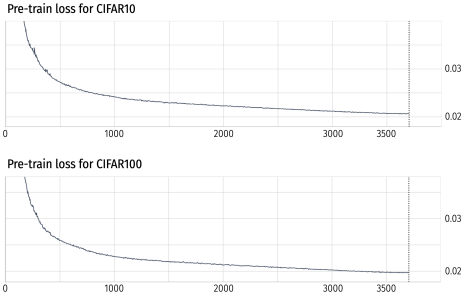
Figure 3: Pre-training loss for both CIFAR-10 and CIFAR-100 datasets. For CIFAR10, the training loss begins at 0.63 and concludes at 0.0207, while for CIFAR100, it starts at 0.66 and finishes at 0.0197. Notably, the y-axis of the plots is limited to the range of around 0.02 to 0.04 to enhance the visibility of the loss trends during most of the epochs. As a result of this scale adjustment, the higher training losses observed in the early epochs are not displayed in this figure.

4.1 On Pre-Training

The models pre-trained on CIFAR-10 and CIFAR-100 are denoted as Mae-ViT-C10 and Mae-ViT-C100, respectively. Pre-training was scheduled for 4000 epochs; however, Mae-ViT-C10 concluded at 3700 epochs, and Mae-ViT-C100 ceased at 3703 epochs due to the end of training sessions. This early stopping was accepted because based on previous observations, there were no significant improvement in loss value noted in the last 300-400 epochs due to the very low learning rates at those epochs.

Pre-training on the more class-diverse CIFAR100 resulted in Mae-ViT-C100 achieving a marginally lower training loss of 0.019711, compared to 0.020733 for Mae-ViT-C10 (refer to Figure 3). While the difference of approximately 0.001 in training loss might seem minor, it is significant in the context of pre-training, where achieving such a reduction often requires hundreds of epochs at later stages. As shown in Figures 4 and 5, the quality of the reconstructed images on visible patches remains high for both models, diverging from the original MAE results [6] due to Eq. 1.

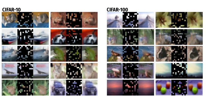
Figure 4: Example results on CIFAR10 and CIFAR100 validation images. For each triplet, on the left is the original image. The middle is the masked image, and the right is the reconstructed image by MAE.

4.2 On Fine-Tuning

Each of the pre-trained models, Mae-ViT-C10 and Mae-ViT-C100, underwent fine-tuning for classification tasks on both CIFAR-10 and CIFAR-100 datasets. The performance results of these models are detailed in Table 3.

All of our models, which were first pre-trained and then fine-tuned, outperformed (in terms of accuracy) comparable transformer architectures that have similar counts of parameters and MACs. The highest accuracy achieved was 96.41% and 78.27% on CIFAR-10 and CIFAR-100 respectively. However, it was observed that models pre-trained and fine-tuned on the same dataset performed better than those pre-trained on one dataset and fine-tuned on the other. On the other hand, in the fine-tuning phase for CIFAR100, signs of overfitting appeared after 50 epochs, whereas this trend was less evident with CIFAR-10 (see Figure 6).

Table 3: Comparison of Top-1 validation accuracy

Model	C10	C100	# Params	MACs
Convolutional Networks (Designed for CIFAR)
ResNet56 [3]	94.63%	74.81%	0.85 M	0.13 G
ResNet110[3]	95.08%	76.63%	1.73 M	0.26 G
ResNet1k-v2* [19]	95.38%	—	10.33 M	1.55 G
Vision Transformers[5]
ViT-12/16	83.04%	57.97%	85.63 M	0.43 G
ViT-Lite-7/16	78.45%	52.87%	3.89 M	0.02 G
ViT-Lite-7/8	89.10%	67.27%	3.74 M	0.06 G
ViT-Lite-7/4	93.57%	73.94%	3.72 M	0.26 G
Compact Vision Transformers[5]
CVT-7/8	89.79%	70.11%	3.74 M	0.06 G
CVT-7/4	94.01%	76.49%	3.72 M	0.25 G
Compact Convolutional Transformers[5]
CCT-2/3 $\times$ 2	89.75%	66.93%	0.28 M	0.04 G
CCT-7/3 $\times$ 2	95.04%	77.72%	3.85 M	0.29 G
MAE Vision Transformers (ours)
Mae-ViT-C10	96.41%	78.20%	3.64 M	0.26 G
Mae-ViT-C100	96.01%	78.27%	3.64 M	0.26 G

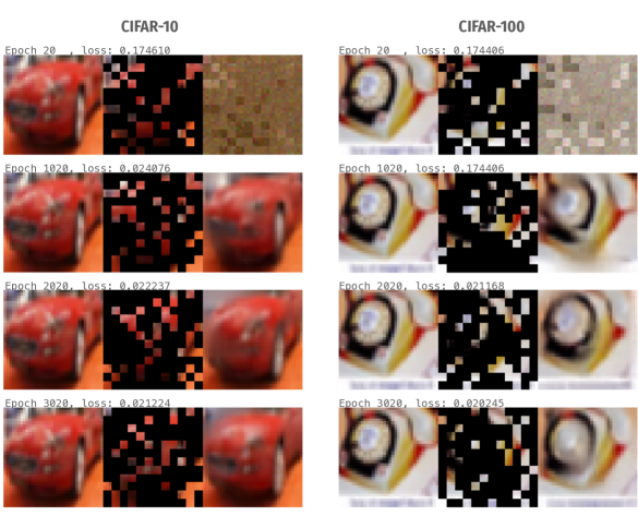
Figure 5: The evolution of the reconstructed outputs by the Masked Auto-Encoder at different training epochs: 20, 1020, 2020, and 3020. The left column displays a sample image from the CIFAR-10 training set, while the right column shows a corresponding sample from the CIFAR-100 training set. Each row corresponds to the reconstruction quality at the specified epoch, demonstrating the progressive refinement of the model’s output over time.

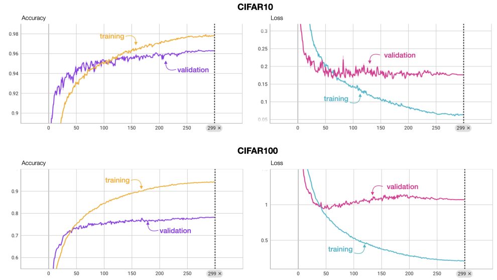
Figure 6: Comparison of training and validation performance for models subjected to both pre-training and fine-tuning on CIFAR-10 and CIFAR-100. The top row features plots of accuracy and loss for the model pre-trained on CIFAR-10 and subsequently fine-tuned on the same dataset. The bottom row follows a similar format, displaying the accuracy and loss for the model pre-trained on CIFAR-100 and fine-tuned on CIFAR-100.

5 Discussion

Table 3 reveals that Vision Transformers (ViT) without pre-training struggle to yield competitive results. It was reported that ViT struggled despite extended training epochs [20]. However, ViTs are sometimes favored due to their computational efficiency on hardware accelerators optimized for large matrix multiplications, which are central to transformer operations, as opposed to the more complex data access patterns required by convolutions [21].

To enhance ViT competitiveness, it’s common to integrate convolutional layers [21, 5] or employ a convolutional ’teacher’ [22] for imparting inductive bias. Our report, however, demonstrates that with a masked auto-encoder setup, these measures are not necessary.

Our models notably outperform standard transformer architectures trained from scratch, as highlighted by the ViT-Lite-7/4 model (see Table 3), which matches our models in parameter count and MACs. They also surpass variations of transformers that incorporate convolutional layers [5], such as CVT-7/4 and CCT-7/3x2. Contrary to most state-of-the-art models that upscale input images (for CIFAR-10 and CIFAR-100), we minimally increase the image size to 36 x 36 from the original 32 x 32, proving the efficacy of vision transformers even with small datasets and resolutions.

The decoders in our lightweight pre-trained models, Mae-ViT-C10 and Mae-ViT-C100, produce satisfactory reconstructions. From our observations, we think a minimum learning rate in the cosine decay schedule could optimize the utility of the final few hundreds epochs, potentially benefiting a subsequent pre-training phase. A tentative minimum learning rate could be around 20% of the value derived from Eq. 2.

MAE proves to be sample-efficient, learning robust representations with less pre-training data and minimizing overfitting compared to other methods [23]. While contrastive methods [24, 25, 26] often lead to stronger representations for the same model size, they face scalability challenges and loss tractability [23]. Pre-trained MAE models require fine-tuning for competitive performance, and while the resulting embeddings have lower linear separability, this does not necessarily correlate with transfer learning performance [27], and linear probing benchmarks are seldom used in natural language processing [6].

In this investigation, we find that models pre-trained on one dataset and fine-tuned on another did not outperform those pre-trained and fine-tuned on the same dataset. This could be due to the insufficient size in the secondary dataset. However, cross-dataset pre-training and fine-tuning did aid in faster convergence, despite the final performance being slightly lower than that of models trained and fine-tuned on the same dataset. In future investigations, it may be beneficial to explore pre-training on a merged dataset that includes both CIFAR-10 and CIFAR-100, followed by fine-tuning on each dataset separately.

6 Conclusion

This report has demonstrated that lightweight ViTs can indeed be pre-trained effectively on small datasets to achieve and even surpass the performance of traditional CNNs. By employing MAE, we have shown that the need for larger datasets or additional convolutional layers, which are commonly believed to be necessary for ViTs to be competitive, can be circumvented.

References

- [1] Yann LeCun, Bernhard Boser, John S Denker, Donnie Henderson, Richard E Howard, Wayne Hubbard, and Lawrence D Jackel. Backpropagation applied to handwritten zip code recognition. Neural computation, 1(4):541–551, 1989.
- [2] Alex Krizhevsky, Ilya Sutskever, and Geoffrey E Hinton. Imagenet classification with deep convolutional neural networks. Advances in neural information processing systems, 25, 2012.
- [3] Kaiming He, Xiangyu Zhang, Shaoqing Ren, and Jian Sun. Deep residual learning for image recognition. In Proceedings of the IEEE conference on computer vision and pattern recognition, pages 770–778, 2016.
- [4] Alexey Dosovitskiy, Lucas Beyer, Alexander Kolesnikov, Dirk Weissenborn, Xiaohua Zhai, Thomas Unterthiner, Mostafa Dehghani, Matthias Minderer, Georg Heigold, Sylvain Gelly, et al. An image is worth 16x16 words: Transformers for image recognition at scale. arXiv preprint arXiv:2010.11929, 2020.
- [5] Ali Hassani, Steven Walton, Nikhil Shah, Abulikemu Abuduweili, Jiachen Li, and Humphrey Shi. Escaping the big data paradigm with compact transformers. arXiv preprint arXiv:2104.05704, 2021.
- [6] Kaiming He, Xinlei Chen, Saining Xie, Yanghao Li, Piotr Dollár, and Ross Girshick. Masked autoencoders are scalable vision learners. In Proceedings of the IEEE/CVF conference on computer vision and pattern recognition, pages 16000–16009, 2022.
- [7] Ashish Vaswani, Noam Shazeer, Niki Parmar, Jakob Uszkoreit, Llion Jones, Aidan N Gomez, Ł ukasz Kaiser, and Illia Polosukhin. Attention is all you need. In I. Guyon, U. Von Luxburg, S. Bengio, H. Wallach, R. Fergus, S. Vishwanathan, and R. Garnett, editors, Advances in Neural Information Processing Systems, volume 30. Curran Associates, Inc., 2017.
- [8] Jimmy Lei Ba, Jamie Ryan Kiros, and Geoffrey E. Hinton. Layer normalization, 2016.
- [9] Jacob Devlin, Ming-Wei Chang, Kenton Lee, and Kristina Toutanova. Bert: Pre-training of deep bidirectional transformers for language understanding. In North American Chapter of the Association for Computational Linguistics, 2019.
- [10] Alex Krizhevsky and Geoffrey Hinton. Learning multiple layers of features from tiny images. Technical Report 0, University of Toronto, Toronto, Ontario, 2009.
- [11] Vinod Nair and Geoffrey E. Hinton. Rectified linear units improve restricted boltzmann machines. In International Conference on Machine Learning, 2010.
- [12] Dan Hendrycks and Kevin Gimpel. Gaussian error linear units (gelus), 2023.
- [13] Nitish Srivastava, Geoffrey Hinton, Alex Krizhevsky, Ilya Sutskever, and Ruslan Salakhutdinov. Dropout: A simple way to prevent neural networks from overfitting. Journal of Machine Learning Research, 15(56):1929–1958, 2014.
- [14] Ilya Loshchilov and Frank Hutter. Decoupled weight decay regularization. In International Conference on Learning Representations, 2019.
- [15] Priya Goyal, Piotr Dollár, Ross Girshick, Pieter Noordhuis, Lukasz Wesolowski, Aapo Kyrola, Andrew Tulloch, Yangqing Jia, and Kaiming He. Accurate, large minibatch sgd: Training imagenet in 1 hour, 2018.
- [16] Ilya Loshchilov and Frank Hutter. SGDR: Stochastic gradient descent with warm restarts. In International Conference on Learning Representations, 2017.
- [17] Kevin Clark, Minh-Thang Luong, Quoc V. Le, and Christopher D. Manning. ELECTRA: pre-training text encoders as discriminators rather than generators. In 8th International Conference on Learning Representations, ICLR 2020, Addis Ababa, Ethiopia, April 26-30, 2020. OpenReview.net, 2020.
- [18] Ekin Dogus Cubuk, Barret Zoph, Dandelion Mane, Vijay Vasudevan, and Quoc V. Le. Autoaugment: Learning augmentation policies from data. In Proceedings of the IEEE/CVF Conference on Computer Vision and Pattern Recognition (CVPR), 2019.
- [19] Kaiming He, Xiangyu Zhang, Shaoqing Ren, and Jian Sun. Identity mappings in deep residual networks. In Computer Vision–ECCV 2016: 14th European Conference, Amsterdam, The Netherlands, October 11–14, 2016, Proceedings, Part IV 14, pages 630–645. Springer, 2016.
- [20] Lei Zhou, Huidong Liu, Joseph Bae, Junjun He, Dimitris Samaras, and Prateek Prasanna. Self pre-training with masked autoencoders for medical image classification and segmentation. In 2023 IEEE 20th International Symposium on Biomedical Imaging (ISBI), pages 1–6. IEEE, 2023.
- [21] Benjamin Graham, Alaaeldin El-Nouby, Hugo Touvron, Pierre Stock, Armand Joulin, Hervé Jégou, and Matthijs Douze. Levit: a vision transformer in convnet’s clothing for faster inference. In Proceedings of the IEEE/CVF international conference on computer vision, pages 12259–12269, 2021.
- [22] Hugo Touvron, Matthieu Cord, Matthijs Douze, Francisco Massa, Alexandre Sablayrolles, and Hervé Jégou. Training data-efficient image transformers & distillation through attention. In International conference on machine learning, pages 10347–10357. PMLR, 2021.
- [23] Alaaeldin El-Nouby, Michal Klein, Shuangfei Zhai, Miguel Angel Bautista, Alexander Toshev, Vaishaal Shankar, Joshua M Susskind, and Armand Joulin. Scalable pre-training of large autoregressive image models. arXiv preprint arXiv:2401.08541, 2024.
- [24] Maxime Oquab, Timothée Darcet, Théo Moutakanni, Huy Vo, Marc Szafraniec, Vasil Khalidov, Pierre Fernandez, Daniel Haziza, Francisco Massa, Alaaeldin El-Nouby, et al. Dinov2: Learning robust visual features without supervision. arXiv preprint arXiv:2304.07193, 2023.
- [25] Jinghao Zhou, Chen Wei, Huiyu Wang, Wei Shen, Cihang Xie, Alan Yuille, and Tao Kong. Image bert pre-training with online tokenizer. In International Conference on Learning Representations, 2021.
- [26] Mathilde Caron, Hugo Touvron, Ishan Misra, Hervé Jégou, Julien Mairal, Piotr Bojanowski, and Armand Joulin. Emerging properties in self-supervised vision transformers. In Proceedings of the IEEE/CVF international conference on computer vision, pages 9650–9660, 2021.
- [27] Xinlei Chen and Kaiming He. Exploring simple siamese representation learning. In Proceedings of the IEEE/CVF conference on computer vision and pattern recognition, pages 15750–15758, 2021.