A unified approach to fluctuations of spectral statistics of generalized patterned random matrices

Abstract.

An $N\times N$ generalized patterned random matrix is a symmetric matrix defined as $A=(x_{L(i,j)}\mathbf{1}_{\Delta}(i,j))$, where $\{x_{k};k\in\mathbb{Z}^{d}\}$ is known as the input sequence, $L:\{1,2,\ldots,N\}^{2}\rightarrow\mathbb{Z}^{d}$ is known as the link function and $\Delta\subseteq\{1,2,\ldots,N\}^{2}$. Several important classes of matrices, including the Wigner matrix, Toeplitz matrix, Hankel matrix, circulant-type matrices and the block versions of these matrices, fall in this category. In 2008, Bose and Sen showed that under some restrictions on the link function $L$ and for $\Delta=\{1,2,\ldots,N\}^{2}$, the corresponding patterned matrices always have a sub-Gaussian limiting spectral distribution [16].

We study the limiting behavior of the linear eigenvalue statistics (LES) of generalized patterned random matrices. Let $N:\mathbb{N}\rightarrow\mathbb{N}$ be a strictly increasing function and $A_{n}=\left(x_{L(i,j)}\mathbf{1}_{\Delta}(i,j)\right)_{i,j=1}^{N(n)}$ be a sequence of generalized patterned matrices. We consider the LES of $A_{n}/\sqrt{N(n)}$ for the test function $\phi(x)=x^{p}$, given by

$$\frac{1}{\sqrt{N(n)}}\sum_{i=1}^{N(n)}\lambda_{i}^{p}=\eta_{p},\mbox{ say},$$

where $p$ is a positive integer and $\lambda_{i}$’s are the eigenvalues of $A_{n}/\sqrt{N(n)}$. Under some restrictions on $L$ and some moment assumptions on input entries, we show that when $p$ is even, $(\eta_{p}-\mathbb{E}[\eta_{p}])$ converges in distribution either to a normal distribution or to the degenerate distribution at zero, as $n\rightarrow\infty$. We show that under further assumptions on $L$, the limit is always a normal distribution. The earlier results on LES of symmetric Toeplitz, Hankel, circulant-type matrices follow as special cases. We also obtain new Gaussian fluctuation results for block Wigner, Toeplitz, Hankel or circulant type matrices matrices, band circulant matrices among others.

For odd degree monomial test functions, we derive the limiting moments for $\eta_{p}$ and show that the LES may not converge to a Gaussian distribution.

We also study the LES of generalized patterned random matrices with independent Brownian motion entries. We show that under some assumption on link function, and that if the limiting moment sequence of the LES of the generalized patterned random matrix with independent standard Gaussian entries is M-determinate, then the LES with Brownian motion entries converge to a deterministic real-valued process.

The key technique in this paper involves extending Lemma 2 from [15], originally formulated for $k=4$, to all positive integers $k$ (see Proposition 24).

Keywords: Linear eigenvalue statistics, patterned random matrix, Toeplitz matrix, Hankel matrix, circulant type matrices, Band matrix, multi-dimensional moment method, central limit theorem, process convergence, Brownian motion. AMS 2020 subject classification: 60B20, 60F05, 60G15.

1. Introduction

1.1. Patterned random matrices

We briefly explain the class of ensembles known as patterned random matrices, whose study was initiated by Bai [4].

Consider a sequence of random variables $\left\{x_{i}:i\in\mathbb{Z}^{d}\right\}$ called the input sequence. For positive integers $N$ and $d$, consider a function $L:\{1,2,\ldots,N\}^{2}\rightarrow\mathbb{Z}^{d}$ called the link function. A link function is called symmetric link function if $L(i,j)=L(j,i)$ for all $1\leq i,j\leq N$. An $N\times N$ patterned matrix with link function $L$ and input sequence $\{x_{i}:i\in\mathbb{Z}^{d}\}$ is defined as $A=\left(x_{L(i,j)}\right)_{i,j=1}^{N}$.

Several important classes of random matrices fall into the category of patterned random matrices with symmetric link functions. A few of the most well-known symmetric patterned random matrices are given below.

1. Wigner matrix $W_{n}^{(s)}$: It is defined as

   $$W_{n}^{(s)}=\left[\begin{array}[]{cccccc}x_{11}&x_{12}&x_{13}&\ldots&x_{1(n-1)}&x_{1n}\\ x_{12}&x_{22}&x_{23}&\ldots&x_{2(n-1)}&x_{2n}\\ \vdots&\vdots&\vdots&\vdots&\vdots&\vdots\\ x_{1n}&x_{2n}&x_{3n}&\ldots&x_{(n-1)n}&x_{nn}\end{array}\right].$$

   Here $L(i,j)=(\min(i,j),\max(i,j))$.

2. Symmetric Toeplitz matrix $T_{n}^{(s)}$: It is defined as

   $$T_{n}^{(s)}=\left[\begin{array}[]{cccccc}x_{0}&x_{1}&x_{2}&\ldots&x_{n-2}&x_{n-1}\\ x_{1}&x_{0}&x_{1}&\ldots&x_{n-3}&x_{n-2}\\ x_{2}&x_{1}&x_{0}&\ldots&x_{n-4}&x_{n-3}\\ \vdots&\vdots&\vdots&\vdots&\vdots&\vdots\\ x_{n-1}&x_{n-2}&x_{n-3}&\ldots&x_{1}&x_{0}\end{array}\right].$$

   Here $L(i,j)=|i-j|$.

3. Hankel matrix $H_{n}$: It is defined as

   $$H_{n}=\left[\begin{array}[]{cccccc}x_{2}&x_{3}&x_{4}&\ldots&x_{n}&x_{n+1}\\ x_{3}&x_{4}&x_{5}&\ldots&x_{n+1}&x_{n+2}\\ x_{4}&x_{5}&x_{6}&\ldots&x_{n+2}&x_{n+3}\\ \vdots&\vdots&\vdots&\vdots&\vdots&\vdots\\ x_{n+1}&x_{n+2}&x_{n+3}&\ldots&x_{2n-1}&x_{2n}\end{array}\right].$$

   Here $L(i,j)=i+j$.

4. Reverse circulant matrix $R_{n}^{(s)}$: It is defined as

   $$R_{n}^{(s)}=\left[\begin{array}[]{cccccc}x_{0}&x_{1}&x_{2}&\ldots&x_{n-2}&x_{n-1}\\ x_{1}&x_{2}&x_{3}&\ldots&x_{n-1}&x_{0}\\ x_{2}&x_{3}&x_{4}&\ldots&x_{0}&x_{1}\\ \vdots&\vdots&\vdots&\vdots&\vdots&\vdots\\ x_{n-1}&x_{0}&x_{1}&\ldots&x_{n-3}&x_{n-2}\end{array}\right].$$

   Here $L(i,j)=(i+j-2)\bmod n.$

Other important types of symmetric patterned random matrices are symmetric circulant matrix, Palindromic Toeplitz matrix and Palindromic Hankel matrix. Each of the above patterned matrices have wide applications in different areas of mathematics, sciences and engineering (see [12],[8], [21] and references therein).

1.2. Block patterned random matrices

A block patterned random matrix has a sequence of patterned matrices as the input sequence instead of random variables. We present the following general technique for the construction of symmetric block patterned matrices studied in this paper. First, we introduce the following definition. Let $A$ and $B$ be patterned random matrices with input sequences $\{x_{i}\}$ and $\{y_{i}\}$, respectively. We say $A$ and $B$ are independent if their input sequences are independent among themselves.

Let $\widetilde{L}:\{1,2,\ldots,M\}^{2}\rightarrow\mathbb{Z}^{d}$ be a function and $\{B_{j}:j\in\mathbb{Z}^{d}\}$ be a sequence of independent (not necessarily symmetric) patterned random matrices of dimension $m\times m$ such that $B_{\widetilde{L}(i,i)}$ is a symmetric matrix for all $1\leq i\leq M$. Define a block patterned matrix with link function $\widetilde{L}$ as the $mM\times mM$ matrix with block structure

$$A=\sum_{i,j=1}^{M}E_{i,j}\otimes\left(\mathbf{1}(i\leq j)B_{\widetilde{L}(i,j)}+\mathbf{1}(i>j)B_{\widetilde{L}(i,j)}^{t}\right),$$ (1)

where $\otimes$ denotes the tensor product, $E_{i,j}$ is the $m\times m$ matrix with $1$ at $(i,j)$ and zero everywhere else, and $\mathbf{1}$ denotes the indicator function. We emphasize that $A$ can be written as a symmetric patterned random matrix with link function depending on the function $\widetilde{L}$ and the link functions of $B_{i}$.

For a concrete construction, consider the following example: Let $B_{0}$ be a Wigner matrix of dimension $m$ with independent standard Gaussian input sequence. Let $\{B_{n}:n\geq 1\}$ be a sequence of independent Ginibre ensembles of dimension $m$. Suppose for each $n\geq 0$, the input sequence of $B_{n}$ is given by $\{x_{n,i,j}:i,j\in\mathbb{Z}\}$. We construct a block Toeplitz matrix of dimension $N=mM$ as the matrix, whose blocks are given by $(T_{n})_{ij}=B_{|i-j|}$ and the corresponding link function is given by

$$L_{n}\left(x,y\right)=\left(|r_{1}-r_{2}|,\min\{s_{1},s_{2}\},\max\{s_{1},s_{2}\}\right),$$

where $x=(r_{1}-1)M+s_{1}$ and $y=(r_{2}-1)M+s_{2}$.

Block versions of patterned random matrices are well-studied in the literature, particularly in operator-valued free probability [47],[51].

1.3. Generalized patterned random matrices

In this work, we look at sequences of symmetric random matrices with increasing dimension constructed in the following way: Setup: For $d\in\mathbb{N}$, consider an input sequence $\{x_{i}:i\in\mathbb{Z}^{d}\}$ and a sequence of symmetric link functions

$$L_{n}:\{1,2,\ldots,N(n)\}^{2}\rightarrow\mathbb{Z}^{d},n\geq 1,$$ (2)

where $N:\mathbb{N}\rightarrow\mathbb{N}$ is a strictly increasing function. We consider the sequence of random matrices of the form

$$(A_{n})_{ij}=\begin{cases}x_{L_{n}(i,j)}&\text{ if }(i,j)\in\Delta_{n},\\ 0&\text{ otherwise},\end{cases}$$ (3)

where $\Delta_{n}$ is a sequence of subsets of $[N]^{2}$ such that $(i,j)\in\Delta_{n}$ implies $(j,i)\in\Delta_{n}$. We call a matrix of the form (3) as a generalized patterned random matrix. Here $[N]$ denotes the set $\{1,2,\ldots,N\}$.

For notational convenience, we shall suppress the dependence of $n$ on $N(n)$ and write $N$ to denote the dimension of the matrix $A_{n}$. We urge the readers to keep in mind that in all cases considered $N$ always depends on $n$ and $N\rightarrow\infty$ as $n\rightarrow\infty$.

Clearly, patterned random matrices considered in the earlier part of this section can be written as (3), by taking $\Delta_{n}=[N]^{2}$. The class of generalized patterned random matrices is much larger. We present a few well known models of random matrices which fall into this class.

1. Let $\{x_{i}:i\in\mathbb{Z}^{2}\}$ be a sequence of independent Bernoulli random variables with parameter $p$, $L_{n}(i,j)=(\min(i,j),\max(i,j))$ and $\Delta_{n}=\{(i,i):0\leq i\leq N\}^{c}$. Then $A_{n}$ is the adjacency matrix of the Erdős-Rényi random graph of $n$ vertices with edge-probability $p$. Further, the adjacency matrices of stochastic block models and inhomogeneous Erdős-Rényi random graph also fall into this category. It is also not hard to see that the unsigned adjacency matrix of the Linial-Meshulam complex, a higher-dimensional generalization of the Erdős-Rényi random graph also fall into this class.

2. Another popular class of matrices of the form (3) are the banded matrices. For a patterned random matrix, two types of banding can be performed. Choosing $\Delta_{n}=\{(i,j):i-b_{n}\leq j\leq i+b_{n},i\in[N]\}$ gives the banding along the diagonal with bandwidth $b_{n}$, and such matrices are called band matrices. Special cases of band matrices include the tridiagonal matrices and pentadiagonal matrices. Choosing $\Delta_{n}=\{(i,j):n+1-b_{n}\leq i+j\leq n+1+b_{n},i\in[N]\}$ gives banding along the anti-diagonal, and such matrices are called anti-diagonal band matrices.

3. Another important subclass is the hollow version of patterned random matrix obtained by choosing $\Delta_{n}=\{(i,i):1\leq i\leq N\}^{c}$, i.e. the diagonal entries are chosen to be zero. Modification of patterned matrices to sparse matrices, skyline matrix and block matrices with zero blocks cases are also of the form (3).

1.4. Spectral distribution

Let $A_{n}$ be an $n\times n$ random matrix with eigenvalues $\lambda_{1,n},\ldots,\lambda_{n,n}$. Then the empirical spectral distribution (ESD) of $A_{n}$ is defined as

$$F_{A_{n}}(x,y)=\frac{1}{n}\#\{k\;:\;\Re(\lambda_{k,n})\leq x,\Im(\lambda_{k,n})\leq y\},\;\;\;\mbox{ for $x,y\in\mathbb{R}$},$$

where $\#$ denotes the cardinality of $A$, and $\Im(x)$ and $\Re(x)$ denote the imaginary and real parts of $x$ respectively. If the ESD of $A_{n}$ converges weakly (a.s. or in probability) to a distribution function $F_{\infty}$ as $n\to\infty$, then the limit is referred to as the limiting spectral distribution (LSD) of $A_{n}$.

A fundamental feature of random matrix theory is that the LSD varies depending on the random matrix. In 1958, Wigner [59] considered symmetric matrices with i.i.d. real Gaussian entries (Wigner matrix) and proved that the LSD is the semicircle law. The LSD of the Gaussian Orthogonal Ensemble (GOE), which models systems with time-reversal symmetry like atomic nuclei, also follows Wigner’s semicircular law. In contrast, the LSD of the sample covariance matrix ($S$-matrix) is the Marcenko-Pastur law [41], of the adjacency matrix of random $d$-regular graphs with large girth is the Kesten-McKay distribution [44].

For Toeplitz and Hankel matrices, Bryc et al. [18] and Hammond, Miller [28] proved the existence of their LSDs. The LSD of reverse circulant matrix is symmetrized Rayleigh distribution [14], and of Palindromic Toeplitz and symmetric circulant matrices is the Gaussian distribution. [42]. Remarkably, despite these diverse LSDs, a consistent behavior emerges: the first order fluctuations of eigenvalues converges to a Gaussian distribution.

1.5. Linear eigenvalue statistics

The study of linear eigenvalue statistics (LES) is also a popular area of research in random matrix theory. For an $n\times n$ matrix $A_{n}$, and a test function $\phi$, the LES of $A_{n}$ is defined as

$$\mathcal{A}_{n}(\phi)=\sum_{i=1}^{n}\phi(\lambda_{i}),$$ (4)

where $\lambda_{1},\lambda_{2},\ldots,\lambda_{n}$ are the eigenvalues of $A_{n}$. Note that if $A_{n}$ is a random matrix, then $\mathcal{A}_{n}(\phi)$ is a random variable. Hence, the obvious question arises about the fluctuations of $\mathcal{A}_{n}(\phi)$ in different mode of convergence. If we suppose $A_{n}(t)$ is a time-dependent random matrix with $t\in[0,\infty)$, where $T$ is an index set, then the LES will be time-dependent, say $\mathcal{A}_{n}(\phi,t)$. Thus, it is natural to study the process convergence (functional convergence or stochastic convergence) of the process $\{\mathcal{A}_{n}(\phi,t);t\in[0,\infty)\}$. A brief discussion on the existing literature of the LES of some important patterned random matrices is given in Section 5.

In this paper, for monomial test functions, we study the LES of generalized patterned random matrices when $\{x_{i}\}$ are either independent random variables obeying some moment assumptions (Assumption I or Assumption II) or independent Brownian motions. Our major result establishes that for even degree monomials, under some reasonable assumptions, the LES of any generalized patterned random matrix converges either to a Gaussian distribution or to the Dirac delta distribution (see Theorem 13). Further, in Theorem 17 we derive an easily verifiable condition for the limit to be a Gaussian random variable. For odd degree monomials, we derive the limiting moment sequence of the LES (Theorem 18). Our results are in confirmation with existing results on LES of the special type of patterned random matrices, namely symmetric Toeplitz, Hankel, circulant-type matrices (see Section 5). We also conclude new results on LES of several other patterned random matrices including versions of Block Toeplitz matrix, Block versions of circulant-type matrices, and $d$-disco matrix with patterned blocks (see Section 5).

The study of matrix-valued stochastic processes is another important problem in random matrix theory starting from the much studied Dyson Brownian motion [24]. For one, such matrices are used in modeling dynamical systems such as the Coulomb gas model [45]. It also introduces the martigale techniques to the study of LES. The study of dynamic CLT for LES is also a popular area of study in random matrix theory, see [2]. For the case of random matrices of type (3) with Brownian motion entries, we show that LES converge to a real-valued process if the LES of the underlying time-independent generalized patterned matrix converges (see Theorem 20).

In the following section, we first state some notations which appear throughout the manuscript and then we state our main results

2. Preliminaries and Main results

2.1. Preliminaries:

In this section, we introduce the basic combinatorial objects required to state our main results.

Definition 1.

Let $[m]=\{1,2,\ldots,m\}$. We call $T=\left\{V_{1},V_{2},\ldots,V_{r}\right\}$ a partition of $[m]$ if the blocks $\{V_{j},1\leq j\leq r\}$ are pairwise disjoint, non-empty subsets of $[m]$ such that $[m]=V_{1}\cup V_{2}\cup\cdots\cup V_{r}$. The number of blocks of $T$ is denoted by $|T|$, and the number of elements of $V_{j}$ is denoted by $\left|V_{j}\right|$. The set of all partitions of $[m]$ is denoted by $\mathcal{P}(m)$.

For a partition $T\in{\mathcal{P}}(m)$ and two elements $i,j\in[m]$ we write $i\sim_{T}j$ if both $i$ and $j$ belong to the same block of $T$. Next, we introduce a few important types of partitions:

Definition 2.

We consider the following type of partitions:

(a) A partition $T=\left\{V_{1},V_{2},\ldots,V_{r}\right\}$ is called a pair-partition if $\left|V_{j}\right|=2,$ for all $1\leq j\leq r$. The set of all pair-partitions of $[m]$, is denoted by $\mathcal{P}_{2}(m)$. Note that $\mathcal{P}_{2}(m)$ is an empty set if $m$ is odd. (b) Suppose $p,q$ are positive integers such that $(p+q)$ is even, we denote a subset of $\mathcal{P}_{2}(p+q)$ by $\mathcal{P}_{2}(p,q)$, which consists of such pair-partitions $T$ : there exist $i,j$ with $1\leq i\leq p<j\leq p+q$ such that $i\sim_{T}j$ (we say that there is at least one cross matching in $T$). (c) When $p$ and $q$ are both even, we denote a subset of $\mathcal{P}(p+q)$ by $\mathcal{P}_{2,4}(p,q)$, which consists of such partitions $T=\left\{V_{1},\ldots,V_{r}\right\}$ satisfying the following conditions:

1. $\left|V_{i}\right|=4$ for some $i$ and $\left|V_{j}\right|=2,$ for all $1\leq j\leq r,j\neq i$,

2. $V_{j}\subseteq\{1,2,\ldots,p\}$ or $\{p+1,p+2,\ldots,p+q\}$ for $1\leq j\leq r,j\neq i$,

3. two elements of $V_{i}$ come from $\{1,2,\ldots,p\}$ and the other two come from $\{p+$ $1,p+2,\ldots,p+q\}$.

For other cases of $p$ and $q$, we assume $\mathcal{P}_{2,4}(p,q)$ is an empty set.

Next, we define the notion of circuits. Recall the definition of link function $L:[N]\rightarrow\mathbb{Z}^{d}$, defined in Section 1.

Definition 3.

Consider a link function $L:[N]\rightarrow\mathbb{Z}^{d}$, where $d\in\mathbb{N}$. A function $\pi:\{0,1,2,\ldots,p\}\rightarrow[N]$ with $\pi(0)=\pi(p)$ is called a circuit of length $p$. Two circuits of length $p$, $\pi_{1}$ and $\pi_{2}$ are said to be equivalent if their $L$-values match at the same locations. That is, for all $1\leq i,j\leq p$,

$$L(\pi_{1}(i-1),\pi_{1}(i))=L(\pi_{1}(j-1),\pi_{1}(j))\Longleftrightarrow L(\pi_{2}(i-1),\pi_{2}(i))=L(\pi_{2}(j-1),\pi_{2}(j)).$$ (5)

The above condition gives an equivalence relation on the set of all circuits of length $p$. It is immediate that any equivalence class can be indexed by a partition of $\{1,2,\ldots,p\}$ where each block of the given partition identifies the positions where the $L$-matches take place. We can label these partitions by words of length $p$ such that the first occurrence of each letter is in alphabetical order. For example, if $p=5$, then the partition $\{\{1,3,5\},\{2,4\}\}$ is represented by the word ababa. This partition identifies all circuits $\pi$ for which $L(\pi(0),\pi(1))=L(\pi(2),\pi(3))=L(\pi(4),\pi(5))$ and $L(\pi(1),\pi(2))=L(\pi(3),\pi(4))$.

Definition 4.

The set of all words $w$ of length $p$ is denoted by $\mathcal{W}_{p}$. The number of distinct letters in $w$ will be denoted by $|w|$.

Note that the set of all words of length $p$ is isomorphic to the set of all partitions of $[p]$ and therefore $\mathcal{W}_{p}$ does not depend on $[N]$, the domain of the link function $L$.

Let $w$ be a word and let $w[i]$ denote the $i$-th letter of $w$. For a link function $L$ and a word $w$, we denote the equivalence class of circuits corresponding to $w$ by

$$\Pi_{L}(w)=\left\{\pi:w[i]=w[j]\Leftrightarrow L(\pi(i-1),\pi(i))=L(\pi(j-1),\pi(j))\right\}.$$

Definition 5.

For $k\geq 1$, a partition of $\{1,2,\ldots,k\}\times\{1,2,\ldots,p\}$ is represented by a sentence with $k$ words each of length $p$. For example, the partition $\{\{(1,1),(2,1)\},\{(1,2),(1,4)\},\{(1,3),(2,4)\},$ $\{(2,2),(2,3)\}\}$ can be represented as $(abcb,addc)$. The set of all sentences of length $k$, with each word having length $p$, is denoted by $\mathcal{W}_{p,k}$. For $k=0$, we take $\mathcal{W}_{p,k}$ as the empty set and for $k=1$, $\mathcal{W}_{p,k}=\mathcal{W}_{p}$.

Note that under the notion of sentences, the partitions in ${\mathcal{P}}_{2}(p,p)$ and ${\mathcal{P}}_{2,4}(p,p)$, defined in Definition 2 can equivalently be considered as sentences in $\mathcal{W}_{p,2}$.

For a link function $L$ and sentence $W=(w_{1},w_{2},\ldots,w_{k})\in\mathcal{W}_{p,k}$, we define

$$\Pi_{L}(W)=\{(\pi_{1},\pi_{2},\ldots,\pi_{k}):w_{r}[i]=w_{s}[j]\Leftrightarrow L(\pi_{r}(i-1),\pi_{r}(i))=L(\pi_{s}(j-1),\pi_{s}(j))\}.$$ (6)

Unfortunately, $\#\Pi_{L}(W)$ is harder to compute and therefore for convenience in computation, we define a slightly larger set $\Pi_{L}^{*}(W)$ given by

$$\Pi_{L}^{*}(W)=\{(\pi_{1},\pi_{2},\ldots,\pi_{k}):w_{r}[i]=w_{s}[j]\implies L(\pi_{r}(i-1),\pi_{r}(i))=L(\pi_{s}(j-1),\pi_{s}(j))\}.$$

It easily follows that if $(\pi_{1},\pi_{2},\ldots,\pi_{k})\in\Pi_{L}(W)$, then $(\pi_{1},\pi_{2},\ldots,\pi_{k})\in\Pi_{L}^{*}(W)$ and therefore $\#\Pi_{L}(W)\leq\#\Pi_{L}^{*}(W)$ for each sentence $W$.

For a set $\Delta\subset[N]^{2}$, we define the following sets

$$\Pi_{L,\Delta}(W) =\{(\pi_{1},\pi_{2},\ldots,\pi_{k})\in\Pi_{L}(W):(\pi_{u}(i-1),\pi_{u}(i))\in\Delta\ \forall\ 1\leq u\leq k,1\leq i\leq p\},$$

$$\Pi^{*}_{L,\Delta}(W) =\{(\pi_{1},\pi_{2},\ldots,\pi_{k})\in\Pi^{*}_{L}(W):(\pi_{u}(i-1),\pi_{u}(i))\in\Delta\ \forall\ 1\leq u\leq k,1\leq i\leq p\}.$$ (7)

Note that in (2.1), the circuits are maps from $\{0,1,\ldots,p\}$ to $[N]$ and hence the cardinality of $\Pi_{L,\Delta}$ depends on $N$ as well. To make the notations simpler, we are suppressing this dependence in the notation.

In general, for a sequence of link functions (given by $L_{n}$) and a sequence of subsets $(\Delta_{n})$, we are interested in finding the cardinality of $\Pi_{L_{n},\Delta_{n}}(W)$. The following inequality directly follows from (2.1) and shall play an important role in computations at later stages.

$$\#\Pi_{L_{n},\Delta_{n}}(W)\leq\#\Pi_{L_{n}}(W)\leq\#\Pi_{L_{n}}^{*}(W)\mbox{ for all $W\in\mathcal{W}_{p,k}$ and $\Delta_{n}\subseteq[N]^{2}$}.$$ (8)

Next, we recall the definition of multi-set.

Definition 6.

A multi-set is a tuple $S=(A,m_{S})$ where $A$ is a set and $m_{S}:A\rightarrow\mathbb{Z}_{+}$ is called the multiplicity function. $A$ is the set of distinct elements in the multi-set and for $a\in A$, $m_{S}(a)$ gives the number of occurrences of $a$ in the multi-set. By a slight abuse in notation, we shall use $a\in S$ to denote that an element $a$ belongs to the underlying set. Throughout the paper for a given multi-set $S$ and $a\in S$, we shall use $m_{S}(a)$ to denote the multiplicity of $a$ in $S$. By convention, $m_{S}(a)=0$ if $a\notin S$.

Consider the following operation defined on multi-sets: For multi-sets $S_{1}=(A_{1},m_{S_{1}})$ and $S_{2}=(A_{2},m_{S_{2}})$, we define the multi-set $S_{1}\uplus S_{2}=\left(A_{1}\cup A_{2},m_{S_{1}}+m_{S_{2}}\right)$, where $\cup$ denotes the usual set union.

Definition 7.

For a word $w\in\mathcal{W}_{p}$, we define by $S_{w}$ the multi-set of letters in $w$. For a sentence $W=(w_{1},w_{2},\ldots,w_{k})\in\mathcal{W}_{p,k}$, we define

$$S_{W}=S_{w_{1}}\uplus S_{w_{2}}\uplus\cdots\uplus S_{w_{k}}.$$

Next, we define the notion of sub-sentences.

Definition 8.

For a sentence $W=(w_{1},w_{2},\ldots,w_{k})\in\mathcal{W}_{p,k}$ and set $\mathcal{C}\subset[k]$, the sub-sentence corresponding to $\mathcal{C}$ is defined as $W_{\mathcal{C}}=(w_{i})_{i\in\mathcal{C}}$.

Now, we define the notion of a graph associated with sentences.

Definition 9.

Let $W=(w_{1},w_{2},\ldots,w_{k})\in\mathcal{W}_{p,k}$ be a sentence. We construct a graph $G_{W}=(V_{W},E_{W})$ associated with $W$ in the following fashion: We define $V_{W}=\{1,2,\ldots,k\}$ and for $r\neq s$, $(r,s)\in E_{W}$ if $S_{w_{r}}\cap S_{w_{s}}\neq\phi$. A maximal connected subgraph of $G_{W}$ is called a cluster.

Note that for any sentence $W$ and any cluster $C$ of $G_{W}$, $G_{W_{C}}=C$. Thus, without loss of generality, for simplicity, we shall represent clusters as the graph of a sentence $W$ such that $G_{W}$ is connected. We now define a special type of cluster called clique cluster.

Definition 10.

For $p\geq 1$ and $k\geq 3$ and $W\in\mathcal{W}_{p,k}$, the graph $G_{W}$ is called a clique cluster if

1. $G_{W}$ is a complete graph, and

2. there exists $a\in S_{W}$ such that for all $i,j\in V$, $S_{w_{i}}\cap S_{w_{j}}=\{a\}$.

A sentence $W\in\mathcal{W}_{p,k}$ is called a clique sentence if $G_{W}$ is a clique cluster, the common letter appears exactly $k$ times and every other letter appear exactly twice in $S_{W}$.

Definition 11.

For $p\geq 1,k\geq 3$, a sentence $W\in\mathcal{W}_{p,k}$ is called a special partition if for each connected component $\mathcal{C}$ of $G_{W}$,

1. $|\mathcal{C}|\geq 2$,

2. if $|\mathcal{C}|=2$, then $W_{\mathcal{C}}$ belongs to either ${\mathcal{P}}_{2}(p,p)$ or ${\mathcal{P}}_{2,4}(p,p)$, and

3. if $|\mathcal{C}|\geq 3$, $W_{\mathcal{C}}$ is a clique sentence.

The set of all special partitions in $\mathcal{W}_{p,k}$ is denoted by $SP(p,k)$.

Observe the following remark from the definition of $SP(p,k)$.

Remark 12.

(a) For even $p$, it can be seen that for any $W\in SP(p,k)$, all clusters of $G_{W}$ has size 2. To observe this, note that if $\mathcal{C}$ is a cluster of size greater than two, then $W_{\mathcal{C}}$ is a clique sentence with common letter say $`c$’. Consider a word $w_{i}$, $i\in{\mathcal{C}}$. By condition (iii) of Definition 11, it follows that $`c$’ appears exactly once in $w_{i}$ and all other letters must appear exactly twice in $w_{i}$. Note that this is possible only when $p$ is odd.
(b) As a consequence of (a), it follows that for $p$ even and $k$ odd, $SP(p,k)$ is empty.

2.2. Main results:

In this section we state our main theorems. We start by stating some assumptions on the input sequence which are necessary to state our results. Both of the below assumptions are standard in the study of LES of random matrices [55], .

Assumption I.

$\left\{x_{i}:i\in\mathbb{Z}^{d}\right\}$ are i.i.d. random variables with mean zero, variance one and $-\infty<\mathbb{E}(x_{i}^{k})=m_{k}<\infty$ for all $k\geq 3$.

Assumption II.

$\{x_{i}:i\in\mathbb{Z}^{d}\}$ are independent random variables with mean zero, variance one, $\mathbb{E}(x_{i}^{4})=\kappa$ for all $i$ and uniformly bounded moments of all order.

Clearly, Assumption I is a stronger assumption when compared to Assumption II. We shall use Assumption I while studying the LES for all monomial function and use Assumption II for studying the special case when the degree of monomial function is even. The reason why we are considering different assumption for different monomial will be clear once we prove the respective result. The following more general assumption on the input sequence is sometimes invoked in the study of the LSD of patterned random matrices.

Assumption III.

$\{x_{i}:i\in\mathbb{Z}^{d}\}$ are independent random variables with mean zero, variance one and uniformly bounded moments of all order.

Next, we introduce an assumption on the sequence of link functions.

Assumption IV.

Let $N:\mathbb{N}\rightarrow\mathbb{N}$ be an increasing function. A sequence of link functions $\{L_{n}:[N(n)]\rightarrow\mathbb{Z}^{d}\}_{n\in\mathbb{N}}$ is said to satisfy Assumption IV if there exists a constant $B<\infty$ such that

$$\sup_{n}\sup_{t\in\mathbb{Z}^{d}}\sup_{1\leq k\leq N(n)}\#\{l:1\leq l\leq N(n),L_{n}(k,l)=t\}\leq B.$$ (9)

A single link function $L:[N]\rightarrow\mathbb{Z}^{d}$ is said to satisfy Assumption IV if the constant sequence $(L_{n}=L\text{ for all }n)$ obeys (9).

Note that all patterned matrices introduced in Section 1 obeys Assumption IV. For example, $B=1$ for the Wigner matrix and reverse circulant matrix, and $B=2$ for symmetric Toeplitz matrix and Hankel matrix.

Our last assumption is on the sequence of sets $\{\Delta_{n}\}_{n\geq 1}$.

Assumption V.

Let $N:\mathbb{N}\rightarrow\mathbb{N}$ be a strictly increasing function and $\Delta_{n}\subseteq[N(n)]^{2}$ for each $n$. We say $\{\Delta_{n}\}$ obeys Assumption V if there exists a set $\Delta\subseteq[0,1]^{2}$ such that $\mathbb{U}_{n}\left((\frac{\Delta_{n}}{N}\setminus\Delta)\cup(\Delta\setminus\frac{\Delta_{n}}{N})\right)$ converges to zero as $n$ goes to infinity, where $\mathbb{U}_{n}$ is the uniform measure on $\{\frac{1}{N},\frac{2}{N},\ldots,1\}^{2}$.

The LSD of random patterned matrices with link function $L$ obeying Assumption IV and input sequence obeying Assumption III was studied by Bose and Sen [16]. They showed that for each $k\in\mathbb{N}$, the $2k$-th moments are due to the contributions from pair-partitions of $\{1,2,\ldots,2k\}$ and as a result, the LSD whenever it exists is sub-Gaussian. The method was generalized to include block patterned random matrices in [6]. We remark here that the results in [16] can be generalized to the matrices of the type (3) also.

In this paper, we derive a unified approach to study the LES of random matrices considered in (3) for monomial test functions. Recall that for $n\in\mathbb{N}$, the dimension of the random matrix $A_{n}$ is $N(n)$, simply written as $N$. In order to study the fluctuations of LES of a random matrix $A_{n}/\sqrt{N}$, where $A_{n}$ is of the form (3), we consider the following scaled and centered version of the LES:

$$\eta_{p}:=\frac{1}{\sqrt{N}}\left(\operatorname{{\mbox{Tr}}}\left(\frac{A_{n}}{\sqrt{N}}\right)^{p}-\mathbb{E}\left[\operatorname{{\mbox{Tr}}}\left(\frac{A_{n}}{\sqrt{N}}\right)^{p}\right]\right).$$ (10)

Note that $\eta_{p}$ depends on $n,\Delta_{n}$ and link function $L_{n}$. To keep the notations simpler, we are not including these dependencies in the notation of $\eta_{p}$. We request the readers to keep in mind these additional dependencies.

Now we state our main results. The following theorem states the result for even degree monomial test functions ($p$ is even).

Theorem 13.

Suppose $\left\{A_{n}=\left(x_{L_{n}(i,j)}{\mathbf{1}}_{\Delta_{n}}(i,j)\right)_{i,j=1}^{N}\right\}$ is a sequence of $N\times N$ symmetric random matrices where

1. the input sequence $\left\{x_{i}\right\}$ satisfies Assumption II,

2. the sequence of link function $\{L_{n}\}$ satisfies Assumption IV,

3. for each sentence $W\in\mathcal{P}_{2}(p,p)\cup\mathcal{P}_{2,4}(p,p)$, the limit $\theta(W)=\lim_{n\rightarrow\infty}\frac{1}{N^{p+1}}\#\Pi_{L_{n},\Delta_{n}}\left(W\right)$ exist, where $\mathcal{P}_{2}(p,p),\mathcal{P}_{2,4}(p,p)$ are as defined in Definition 2 and $\Pi_{L_{n},\Delta_{n}}(W)$ is as defined in (2.1).

Then for even $p$,

$$\eta_{p}\stackrel{{\scriptstyle d}}{{\longrightarrow}}\left\{\begin{array}[]{ll}\displaystyle N\left(0,\sigma_{p}^{2}\right)&\text{if }\sigma_{p}>0,\\ \displaystyle 0&\text{if }\sigma_{p}=0,\end{array}\right.$$

where

$$\sigma_{p}^{2}=\sum_{W\in{\mathcal{P}}_{2}(p,p)}\theta\left(W\right)+(\kappa-1)\sum_{W\in{\mathcal{P}}_{2,4}(p,p)}\theta\left(W\right).$$

Corollary 14.

If we consider $\Delta_{n}=[N]^{2}$, then Theorem 13 provides the LES results for symmetric patterned random matrices.

Remark 15.

(a) Condition (iii) of Theorem 13 can alternatively be replaced with the weaker assumption

$$\lim_{n\rightarrow\infty}\Big{[}\sum_{W\in{\mathcal{P}}_{2}(p,p)}\#\Pi_{L_{n},\Delta_{n}}\left(W\right)+(\kappa-1)\sum_{W\in{\mathcal{P}}_{2,4}(p,p)}\#\Pi_{L_{n},\Delta_{n}}\left(W\right)\Big{]}$$

exist, where $\Pi_{L_{n},\Delta_{n}}$ is as in (2.1). The above expression is the limiting second moment of $\eta_{p}$. Hence, condition (iii) can also be replaced by $\lim_{n\to\infty}\mathbb{E}[\eta_{p}^{2}]$ exist. This is a considerable relaxation of assumptions compared to the results in [16]. In [16], to prove the existence of the LSD, the existence of all limiting moments of ESD needs to be assumed, whereas in this case, only the convergence of the second moment is enough. (b) It is known from [37] that for random symmetric Toeplitz matrices, for all sentences $W$ in $\mathcal{P}_{2}(p,p)$ and $\mathcal{P}_{2,4}(p,p)$, $\theta(W)$ is non-zero.

Theorem 13 prompts an immediate inquiry: Does there exist an easily verifiable condition for the limit of LES to be Gaussian? Our next theorem provides exactly that. To state the result, first we introduce the following convention:

Notation 16.

For $n\in\mathbb{N}$ and a link function $L_{n}$, we define the following non-empty sequences of sets

• $\mathcal{Z}_{n}=\{r_{1},r_{2},\ldots\}$ is any non-empty subset of $\operatorname{Im}(L_{n})$, where $\operatorname{Im}(L_{n})$ denotes the image set of $L_{n}$.

• For $\mathcal{Z}_{n}\subseteq\operatorname{Im}(L_{n})$, consider $\mathcal{S}_{n}\subset\{(i,j)\in\Delta_{n}:L_{n}(i,j)=r_{u}\text{ for some }r_{u}\in\mathcal{Z}_{n}\}$ such that $(i,j)\in\mathcal{S}_{n}\implies(j,i)\in\mathcal{S}_{n}$.

The hardest part in applying Theorem 13 is showing that condition (iii) holds. But under the assumption that $\{\Delta_{n}\}$ obeys Assumption V, it follows that this condition holds for some of the most well-known link functions. For more details see Section 5.1.

The following theorem gives a sufficient condition based only on the link functions $\{L_{n}\}$ for the LES to converge to a normal distribution.

Theorem 17.

Suppose $\left\{A_{n}=\left(x_{L_{n}(i,j)}{\mathbf{1}}_{\Delta_{n}}(i,j)\right)_{i,j=1}^{N}\right\}$ is a sequence of $N\times N$ symmetric random matrices obeying all assumptions of Theorem 13. Additionally, assume that there exist constants $c_{1},c_{2}>0$ and non-empty sets $\mathcal{Z}_{n}\subseteq\operatorname{Im}(L_{n})$ such that

1. for each $n\in\mathbb{N}$ and $r_{u}\in\mathcal{Z}_{n}$, $\#\{(i,j)\in\mathcal{S}_{n}:L_{n}(i,j)=r_{u}\}\geq c_{1}N$,

2. if for some row $R_{i}$ of the matrix $A_{n}$, $\mathcal{S}_{n}\cap R_{i}\neq\phi$, then $\#(\mathcal{S}_{n}\cap R_{i})\geq c_{2}N$.

Then for each even $p$, $\sigma_{p}^{2}$ given in Theorem 13 is strictly positive. As a consequence, $\eta_{p}$ defined in (10) converges in distribution to a normal distribution with mean 0 and variance $\sigma_{p}^{2}$.

Even though it might not be immediately clear, the conditions of Theorem 17 can be easily verified. We dedicate Section 5 in verifying the conditions for link functions of several well-known patterned matrices. We show that the variations of several classes of important patterned random matrices such as symmetric Toeplitz, Hankel, symmetric circulant, reverse circulant and their block versions obey the conditions of Theorem 17. As a result, for each of the above matrix, and for each even $p$, $\eta_{p}$ defined in (10) converges in distribution to a normal distribution with mean 0.

Next, we deal with the LES of generalized patterned random matrices for odd degree monomial test function ($p$ is odd).

Theorem 18.

Suppose $\left\{A_{n}=\left(x_{L_{n}(i,j)}{\mathbf{1}}_{\Delta_{n}}(i,j)\right)_{i,j=1}^{N}\right\}$ is a sequence of $N\times N$ symmetric random matrices where

1. the input sequence $\{x_{i}:i\in\mathbb{Z}^{d}\}$ satisfies Assumption I,

2. the sequence of link function $\{L_{n}\}$ satisfies Assumption IV,

3. for each sentence $W\in SP(p,k)$, the limit $\theta(W)=\lim_{n\rightarrow\infty}\frac{1}{N^{\frac{pk+k}{2}}}\#\Pi_{L_{n},\Delta_{n}}\left(W\right)$ exist.

Then for odd $p$, the limiting moments of $\eta_{p}$ are given by

$$\lim_{n\rightarrow\infty}\mathbb{E}\left[\eta_{p}^{k}\right] =\displaystyle\sum_{W\in SP(p,k)}\prod_{i=1}^{s}m_{r_{i}}\theta(W_{C_{i}}),$$ (11)

where $``s"$ is the number of clusters of $G_{W}$ (as defined in Definition 9), $r_{i}=|C_{i}|$ is the size of the $i^{th}$ cluster, $m_{r_{i}}$ is as in Assumption I, $W_{C_{i}}$ is as given in Definition 8, and $SP(p,k)$ is defined as in Definition 11.

Remark 19.

In Theorem 18, only the limiting moments are calculated. To conclude convergence in distribution using moment method, it is additionally required to show that the limiting moment sequence uniquely determine a distribution (i.e. the moment sequence is M-determinate). But that does not hold for all patterned random matrices. For symmetric circulant matrix, the limiting moment sequence is M-determinate, in fact the limit is Gaussian, see [43]. Whereas for symmetric Toeplitz matrix, the limiting moment sequence does not uniquely determine a distribution (M-indeterminate), see [37]. Hence convergence in distribution cannot be concluded for all matrices of the form (3). In Theorem 18, if we additionally assume that the limiting moment sequence is M-determinate, say with distribution $\mathcal{F}$, then $\eta_{p}$ converges in distribution to $\mathcal{F}$.

In the last part of this article, we deal with the LES of random matrices of form (3) with independent Brownian motion entries. We introduce the necessary terminology to study generalized patterned random matrices with independent Brownian motion entries under a unified framework.

Let $\{a_{i}(t):t\geq 0,\ i\in\mathbb{Z}^{d}\}$ be a sequence of independent Brownian motions. We define the matrix-valued stochastic process corresponding to link function $L_{n}$ and a subset $\Delta_{n}\subset[N]^{2}$, as

$$A_{n}(t)=\left(a_{L_{n}(i,j)}(t){\mathbf{1}}_{\Delta_{n}}(i,j)\right)_{i,j=1}^{N}.$$

Here we establish connections between time-dependent fluctuations and time-independent fluctuations of LES for generalized patterned random matrices. For a matrix-valued stochastic process $A_{n}(t)$ with the link function $L_{n}$ and an input sequence of stochastic process $\{a_{i}(t)\}$, we define

$$\kappa_{p}(t):=\frac{1}{\sqrt{N}}\left[{\mbox{Tr}}\left(\frac{A_{n}(t)}{\sqrt{N}}\right)^{p}-\mathbb{E}{\mbox{Tr}}\left(\frac{A_{n}(t)}{\sqrt{N}}\right)^{p}\right].$$ (12)

Similarly, corresponding to $A_{n}(t)$, the time-independent LES is

$$\kappa_{p}:=\frac{1}{\sqrt{N}}\left[{\mbox{Tr}}\left(\frac{A_{n}(1)}{\sqrt{N}}\right)^{p}-\mathbb{E}{\mbox{Tr}}\left(\frac{A_{n}(1)}{\sqrt{N}}\right)^{p}\right].$$ (13)

Here the input sequence consists of time-independent random variables $\{x_{i}\}$ which has same distribution as $N(0,1)$. The objective of the second part of this paper is to build connection between the random variable $\kappa_{p}$ and the process $\kappa_{p}(t)$ when the input stochastic process $\{a_{i}(t)\}$ are independent Brownian motions. The following theorem provides the result:

Theorem 20.

Let $\{A_{n}(t)=\left(a_{L_{n}(i,j)}(t){\mathbf{1}}_{\Delta_{n}}(i,j)\right)_{i,j=1}^{N}\}$ be a sequence of matrix-valued stochastic processes such that conditions (ii) and (iii) of Theorem 18 holds. Additionally, suppose that for a fixed positive integer $p$, that the limiting moment sequence of $\kappa_{p}$ is M-determinate. Then there exists a real-valued continuous process $\big{\{}\Gamma_{p}(t);t\geq 0\big{\}}$ such that

$$\big{\{}\kappa_{p}(t);t\geq 0\big{\}}\stackrel{{\scriptstyle\mathcal{D}}}{{\rightarrow}}\big{\{}\Gamma_{p}(t);t\geq 0\big{\}}.$$ (14)

Moreover if the limiting distribution of $\kappa_{p}$ is Gaussian, then the limiting process $\big{\{}\Gamma_{p}(t);t\geq 0\big{\}}$ is a Gaussian process.

Remark 21.

(a) Similar to Corollary 14, in particular for $\Delta_{n}=[N]^{2}$, Theorems 17 and 20 provide the LES results for symmetric patterned random matrices.

(b) If we define

$$\kappa_{c,p}(t):=\frac{1}{N^{c(p)}}\left[{\mbox{Tr}}\left(\frac{A_{n}(t)}{\sqrt{N}}\right)^{p}-\mathbb{E}{\mbox{Tr}}\left(\frac{A_{n}(t)}{\sqrt{N}}\right)^{p}\right],$$

then Theorem 20 holds for such process whenever $c(p)\leq 1/2$, where $c(p)$ is a constant that depends on $p$, but is independent of $n$. It often happens that for a same type of matrix the constant $c(p)$ is different for odd and even $p$.

Now we briefly outline the structure of the rest of this manuscript. In Section 3, we provide a sketch of the idea used to deal with the LES of any generalized patterned random matrix, and then we prove Theorems 13, 17 and 18. In Section 4, we prove some results that form the backbone of the unified technique. Section 5 shows how our results provide some existing and new results for the LES of several random matrices. Finally, in Section 6, we prove Theorem 20.

3. LES for independent entries

In this section, we present a unified technique to derive the limiting moment sequence of the LES of any symmetric generalized patterned random matrix and any monomial test function. In Section 3.1, we provide a unified technique to deal with the limiting moment sequence for LES of any generalized patterned random matrix. In Sections 3.2, 3.3 and 3.4, we prove Theorems 13, 18 and 17, respectively.

3.1. General setup for independent entries:

We first sketch the idea behind our approach. Let $\eta_{p}$ be as defined in (10). First, we discuss how $\eta_{p}$ can be connected to the sets $\Pi_{L}(W)$ defined in (6). Recall the definition of circuit from Definition 3. From (10) it follows that for all $k\in\mathbb{N}$,

$$\eta_{p}^{k}=\frac{1}{N^{\frac{pk+k}{2}}}\displaystyle\sum_{\pi_{1},\ldots,\pi_{k}}\big{[}(x_{\pi_{1}}-\mathbb{E}x_{\pi_{1}})(x_{\pi_{2}}-\mathbb{E}x_{\pi_{2}})\cdots(x_{\pi_{k}}-\mathbb{E}x_{\pi_{k}})\prod_{u=1,2,\ldots,k\atop i=1,2,\ldots,p}{\mathbf{1}}_{\Delta_{n}}(\pi_{u}(i-1),\pi_{u}(i))\big{]}.$$ (15)

where for $d=1,2,\ldots,k$; $\pi_{d}:\{0,1,2,\ldots,p\}\rightarrow\{1,2,\ldots,N\}$ are circuits of length $p$, and $x_{\pi_{d}}$ is defined as

$$x_{\pi_{d}}=x_{L_{n}(\pi_{d}(0),\pi_{d}(1))}x_{L_{n}(\pi_{d}(1),\pi_{d}(2))}\cdots x_{L_{n}(\pi_{d}(p-1),\pi_{d}(p))}.$$

Note that $\mathbb{E}(\eta_{p})=0$. For $k\geq 2$, using the relation (2.1) between sentences and circuits, we have

$$\mathbb{E}(\eta_{p}^{k}) =\frac{1}{N^{\frac{(p+1)k}{2}}}\sum_{W\in\mathcal{W}_{p,k}}\sum_{\Pi_{L_{n},\Delta_{n}}(W)}\mathbb{E}\big{(}\prod_{i=1}^{k}(x_{\pi_{i}}-\mathbb{E}x_{\pi_{i}})\big{)}$$

$$=\frac{1}{N^{\frac{(p+1)k}{2}}}\Big{[}\sum_{W\in SP(p,k)}\sum_{\Pi_{L_{n},\Delta_{n}}(W)}\mathbb{E}\big{(}\prod_{i=1}^{k}(x_{\pi_{i}}-\mathbb{E}x_{\pi_{i}})\big{)}+\sum_{W\notin SP(p,k)}\sum_{\Pi_{L_{n},\Delta_{n}}(W)}\mathbb{E}\big{(}\prod_{i=1}^{k}(x_{\pi_{i}}-\mathbb{E}x_{\pi_{i}})\big{)}\Big{]}$$

$$=\theta_{1}+\theta_{2},\mbox{ say},$$ (16)

where $\Pi_{L_{n},\Delta_{n}}(W)$ is as in (2.1); $(\pi_{1},\pi_{2},\ldots,\pi_{k})\in\Pi_{L_{n},\Delta_{n}}(W)$, and $\mathcal{W}_{p,k},SP(p,k)$ are as defined in Definitions 5, 11, respectively.

The first step in proving Theorems 13 and 18 is to show that

$$\theta_{2}=o(1).$$ (17)

Before going into the details of proving (17), we make the following observations.

1. If there exists $\pi_{t}$ which is not connected with any other $\pi_{s}$ (i.e. $\operatorname{Im}(\pi_{t})\cap\operatorname{Im}(\pi_{s})=\phi$ for all $s$), then due to the independence of the input sequence, the expectation term will be zero.

2. The same conclusion is true also if a letter appears only once in the sentence $W$.

Consequently, the expectation in (3.1) will be non-zero only if each letter in $S_{W}$ is repeated at least twice and each cluster has size greater than or equal to two.

Also, observe that the quantity $\mathbb{E}\big{(}\prod_{i=1}^{k}(x_{\pi_{i}}-\mathbb{E}x_{\pi_{i}})\big{)}$ is uniformly bounded for all sentences $W\in\mathcal{W}_{p,k}$, if the input entries obeys one of Assumption I or Assumption II. Therefore

$$|\theta_{2}|\leq\frac{1}{N^{\frac{pk+k}{2}}}\sum_{W\notin SP(p,k)}\sum_{\Pi_{L_{n},\Delta_{n}}(W)}|\mathbb{E}\big{(}\prod_{i=1}^{k}(x_{\pi_{i}}-\mathbb{E}x_{\pi_{i}})\big{)}|\leq\frac{1}{N^{\frac{pk+k}{2}}}\sum_{W\notin SP(p,k)}M_{W}\#\Pi_{L_{n},\Delta_{n}}^{*}(W),$$

where $M_{W}$ is a constant that depends only on the sentence $W$. Hence proving (17) is equivalent to proving that

$$\#\Pi_{L_{n},\Delta_{n}}(W)=o(N^{\frac{pk+k}{2}}),$$ (18)

for all sentences $W\notin SP(p,k)$, with each letter in $S_{W}$ repeating at least twice and each cluster of $W$ having size greater than two.

Let $W$ be a sentence such that $G_{W}$ has clusters $C_{1},C_{2},\ldots,C_{m}$ with $\#V(C_{i})=k_{i}$. Then we have

$$\frac{1}{N^{\frac{pk+k}{2}}}\#\Pi_{L_{n},\Delta_{n}}^{*}(W)=\prod_{i=1}^{m}\frac{1}{N^{\frac{pk_{i}+k_{i}}{2}}}\#\Pi_{L_{n},\Delta_{n}}^{*}(W_{C_{i}}),$$

where $W_{C_{i}}$ is as defined in Definition 8. Hence, it is sufficient to look at the contributions of sentences $W$ such that $G_{W}$ is connected.

Recall from (8) that $\#\Pi_{L_{n},\Delta_{n}}(W)\leq\#\Pi_{L_{n}}^{*}(W)$ for all sentences $W$. The following proposition states that the contribution of these cases are bounded.

Proposition 22.

Let $\{L_{n}:{[N(n)]^{2}\rightarrow\mathbb{Z}^{d}}\}$ be a sequence of link functions obeying Assumption IV.

1. For every sentence $W\in SP(p,2)=\mathcal{P}_{2}(p,p)\cup\mathcal{P}_{2,4}(p,p)$,

   $$\frac{1}{N^{p+1}}\#\Pi_{L_{n}}(W)\leq\frac{1}{N^{p+1}}\#\Pi_{L_{n}}^{*}(W)=O(1).$$ (19)

   For all other $W\in\mathcal{W}_{p,2}\setminus SP(p,2)$ with at least one cross-matched element, and each element in $S_{W}$ appearing at least twice,

   $$\frac{1}{N^{p+1}}\#\Pi_{L_{n}}^{*}(W)=o(1).$$

2. For $k\geq 3$, let $W\in\mathcal{W}_{p,k}$ be a clique sentence. Then

   $$\frac{1}{N^{\frac{pk+k}{2}}}\#\Pi_{L_{n}}(W)=O(1),$$

   where the notion clique sentence is as defined in Definition 10.

We make the following remark using Proposition 22 (a).

Remark 23.

Let $\{L_{n}:{[N(n)]^{2}\rightarrow\mathbb{Z}^{d}}\}$ be a sequence of link functions obeying Assumption IV.

1. For every sentence $W\in\mathcal{P}_{2,4}(p,p)$, note that the set $\Pi_{L_{n}}^{*}(W)\setminus\Pi_{L_{n}}(W)$ is can be given by

   $$\Pi_{L_{n}}^{*}(W)\setminus\Pi_{L_{n}}(W)=\bigcup_{\tilde{W}}\Pi_{L_{n}}(\tilde{W}),$$

   where $\tilde{W}$ is obtained by taking different letters of $W$ to be the same. Also observe that each $\tilde{W}$ in the above union is not an element of ${\mathcal{P}}_{2,4}(p,p)\cup{\mathcal{P}}_{2}(p,p)$ and hence by Proposition 22 (a),

   $$\lim_{n\rightarrow\infty}\frac{1}{N^{p+1}}\#\Pi_{L_{n}}(W)=\lim_{n\rightarrow\infty}\frac{1}{N^{p+1}}\#\Pi_{L_{n}}^{*}(W),$$

   provided at least one of them exists.

2. For $W\in{\mathcal{P}}_{2}(p,p)$, the above observation does not necessarily hold.

Having deduced that the contribution of the above clusters is bounded, we have reduced proving (17) to proving the following proposition.

Proposition 24.

Let $\{L_{n}\}$ be a sequence of link functions obeying Assumption IV. For $p\geq 1$ and $k\geq 3$, let $W=(w_{1},w_{2},\ldots,w_{k})\in\mathcal{W}_{p,k}$ be such that each letter in $S_{W}$ is repeated at least twice. If $G_{W}$ is connected but not a clique sentence, then

$$\frac{1}{N^{\frac{pk+k}{2}}}\#\Pi_{L_{n}}^{*}(W)=o(1).$$

Proposition 24 is the backbone of this paper. The proof for Proposition 24 is a bit long and involves some ideas from graph theory. For now, we shall skip the proofs of Propositions 22 and 24, and move on to proving the main theorems, assuming that the propositions are true. The proofs of Propositions 22 and 24 are given in Section 4.

3.2. Proof of Theorems 13:

With the help of the above propositions, we prove Theorem 13 using the method of moments and Wick formula.

Proof of Theorem 13.

Let $p$ be an even positive integer. Recall from (3.1) that

$$\mathbb{E}(\eta_{p}^{k})$$

$$=\frac{1}{N^{\frac{(p+1)k}{2}}}\Big{[}\sum_{W\in SP(p,k)}\sum_{\Pi_{L_{n},\Delta_{n}}(W)}\mathbb{E}\big{(}\prod_{i=1}^{k}(x_{\pi_{w_{i}}}-\mathbb{E}x_{\pi_{w_{i}}})\big{)}+\sum_{W\notin SP(p,k)}\sum_{\Pi_{L_{n},\Delta_{n}}(W)}\mathbb{E}\big{(}\prod_{i=1}^{k}(x_{\pi_{w_{i}}}-\mathbb{E}x_{\pi_{w_{i}}})\big{)}\Big{]},$$

where $SP(p,k)$ is as defined in Definition 11. Observe from the discussions in Section 3.1, that the second term in the above expression has zero contribution in the limit. Now, we inspect the elements of $SP(p,k)$. From Remark 12, we have that for odd $k$, $SP(p,k)$ is empty. Therefore for all $k\in\mathbb{N}$,

$$\lim_{n\rightarrow\infty}\mathbb{E}\left(\eta_{p}^{2k+1}\right)=0.$$

Now we focus on the even moments of $\eta_{p}$. Consider a sentence $W\in SP(p,2k)$. It follows from Remark 12 that each cluster of $W$ belongs to ${\mathcal{P}}_{2}(p,p)$ or ${\mathcal{P}}_{2,4}(p,p)$. Thus each letter in $S_{W}$ appears either exactly twice or exactly four times. Note that the input entries $\{x_{i}\}$ obeys Assumption II, implying the independence of $\{x_{i}\}$ and the homogeneity of the second and fourth moments. Hence for every $W\in SP(p,2k)$, the value of

$$\mathbb{E}\left[(x_{\pi_{1}}-\mathbb{E}(x_{\pi_{1}}))(x_{\pi_{2}}-\mathbb{E}(x_{\pi_{2}}))\cdots(x_{\pi_{2k}}-\mathbb{E}(x_{\pi_{2k}}))\right]$$

is fixed for all $(\pi_{1},\pi_{2},\ldots,\pi_{2k})\in\Pi_{L_{n},\Delta_{n}}(W)$, and we shall denote

$$\mathbb{E}\left[\prod_{i=1}^{2k}(x_{\pi_{i}}-\mathbb{E}(x_{\pi_{i}}))\right]=\mathbb{E}\left[\prod_{i=1}^{2k}(x_{{w_{i}}}-\mathbb{E}(x_{{w_{i}}}))\right].$$

Using this observation and proposition 24, we deduce that

$$\mathbb{E}\left(\eta_{p}^{2k}\right)=\frac{1}{N^{pk+k}}\sum_{W\in SP(p,2k)}\prod_{C:\text{ cluster}\atop\text{of }W}\mathbb{E}\left(\prod_{i\in V(C)}(x_{{w_{i}}}-\mathbb{E}x_{{w_{i}}})\right)\#\Pi_{L_{n},\Delta_{n}}(W)+o(1),$$ (20)

where $V(C)$ denotes the vertex set of $C$.

Recall that for even $p$ and a sentence $W\in SP(p,2k)$, all clusters of $G_{W}$ belong to one of $\mathcal{P}_{2}(p,p)$ or $\mathcal{P}_{2,4}(p,p)$. Consider $W_{C}=(w_{1}^{\prime},w_{2}^{\prime})\in\mathcal{P}_{2}(p,p)$, then there exists $a\in S_{W_{C}}$ such that $a$ is repeated only once both in $S_{w_{1}^{\prime}}$ and in $S_{w_{2}^{\prime}}$. Thus it follows that $\mathbb{E}(w_{1}^{\prime})=0=\mathbb{E}(w_{2}^{\prime})$. Therefore

$$\mathbb{E}\left(\prod_{i\in V(C)}(x_{{w_{i}}}-\mathbb{E}x_{{w_{i}}})\right)=\mathbb{E}[x_{w_{1}^{\prime}}x_{w_{2}^{\prime}}]=1.$$

For $W_{C}=(w_{1}^{\prime},w_{2}^{\prime})\in\mathcal{P}_{2,4}(p,p)$, note that each letter $a\in S_{w_{i}^{\prime}}$ is repeated exactly twice in $S_{w_{i}^{\prime}}$. Furthermore, $S_{w_{1}^{\prime}}\cap S_{w_{2}^{\prime}}$ contains only one letter, which is repeated exactly four times in $S_{W_{C}}$. Therefore,

$$\mathbb{E}\left(\prod_{i\in V(C)}(x_{{w_{i}}}-\mathbb{E}x_{{w_{i}}})\right) =\mathbb{E}\left((x_{{w_{1}^{\prime}}}-1)(x_{{w_{2}^{\prime}}}-1)\right)=\mathbb{E}(x_{{w_{1}^{\prime}}}x_{{w_{2}^{\prime}}}-x_{{w_{1}^{\prime}}}-x_{{w_{2}^{\prime}}}-1)=\kappa-1.$$

Note that each sentence in $SP(p,2k)$ are composed of $k$ sub-sentences of two words. Suppose sentences $W_{C_{1}},W_{C_{2}},\ldots,W_{C_{k}}$ are given, with $r$ sentences in ${\mathcal{P}}_{2}(p,p)$ and the rest $(k-r)$ sentences belonging to ${\mathcal{P}}_{2,4}(p,p)$. We aim to enumerate the number of sentences $W\in SP(p,2k)$ such that sentences $W_{C_{1}},\ldots,W_{C_{k}}$ are the sub-sentences corresponding to the clusters of $W$ . Note that the number of ways of choosing $k$ clusters of size two is $\#{\mathcal{P}}_{2}(2k)$, the number of pair-partitions of $[2k]$. And the number of ways of choosing $r$ clusters among this particular choice of $k$ clusters, such that the corresponding sub-sentences are elements of ${\mathcal{P}}_{2}(p,p)$, is ${k\choose r}$. Once, the above are fixed, we can uniquely determine the sentence $W\in SP(p,2k)$. This implies that

$$\lim_{n\rightarrow\infty}\mathbb{E}\left(\eta_{p}^{2k}\right)$$

$$=\lim_{n\rightarrow\infty}\frac{1}{N^{pk+k}}\#\mathcal{P}_{2}(2k)\sum_{r=0}^{k}\sum_{W_{1},\ldots,W_{r}\in\mathcal{P}_{2}(p,p)\atop W_{r+1},\ldots,W_{k}\in\mathcal{P}_{2,4}(p,p)}{k\choose r}\prod_{i=1}^{k}\mathbb{E}\left(\prod_{j=1,2}(x_{{w_{i}^{(j)}}}-\mathbb{E}x_{w_{i}^{(j)}})\right)\#\Pi_{L_{n},\Delta_{n}}(W),$$ (21)

where $W_{i}=(w_{i}^{(1)},w_{i}^{(2)})$ and $W=(W_{1},W_{2},\ldots,W_{k})$.

Next note that, since $p$ is even, if two different letters from different clusters correspond to the same $L_{n}$-value, then we have that the sentence is not element of $SP(p,k)$. Therefore by Proposition 24, we get that

$$\lim_{n\rightarrow\infty}\#\Pi_{L_{n},\Delta_{n}}(W)=\lim_{n\rightarrow\infty}\prod_{i=1}^{k}\#\Pi_{L_{n},\Delta_{n}}(W_{i}).$$

Further from condition $(iii)$ of Theorem 13, it follows that

$$\lim_{n\to\infty}\frac{1}{N^{pk+k}}\#\Pi_{L_{n},\Delta_{n}}(W_{i})=\theta(W_{i}),$$

exist for all $1\leq i\leq k$. Now from (3.2), using the substitution of the value of the expectation term, it follows that

$$\lim_{n\to\infty}\mathbb{E}\left(\eta_{p}^{2k}\right) =\#\mathcal{P}_{2}(2k)\displaystyle\sum_{r=1}^{k}\sum_{W_{1},\ldots,W_{r}\in\mathcal{P}_{2}(p,p)\atop W_{r+1},\ldots,W_{k}\in\mathcal{P}_{2,4}(p,p)}{k\choose r}(\kappa-1)^{k-r}\prod_{i=1}^{k}\theta(W_{i}).$$

Now observe from the above expression that,

$$\lim_{n\rightarrow\infty}\mathbb{E}[\eta_{p}^{2}]=\displaystyle\sum_{{W}_{1}\in\mathcal{P}_{2}(p,p)}\theta({W}_{1})+\sum_{{W}_{2}\in\mathcal{P}_{2,4}(p,p)}(\kappa-1)\theta({W}_{2})=\sigma_{2}^{2},\mbox{ say}.$$

For $k\in\mathbb{N}$, let $\beta_{k}=\lim_{n\rightarrow\infty}\mathbb{E}[\eta_{p}^{k}]$. Then from the above calculations, we have $\beta_{k}=0$ for odd $k$ and

$$\beta_{2k}=\lim_{n\rightarrow\infty}\mathbb{E}[\eta_{p}^{2k}] =\#\mathcal{P}_{2}(2k)\displaystyle\sum_{r=0}^{k}{k\choose r}(\kappa-1)^{k-r}\left(\sum_{{W}_{1}\in\mathcal{P}_{2}(p,p)}\theta({W}_{1})\right)^{r}\left(\sum_{{W}_{2}\in\mathcal{P}_{2,4}(p,p)}\theta({W}_{2})\right)^{k-r}$$

$$=\#\mathcal{P}_{2}(2k)\left(\sum_{{W}_{1}\in\mathcal{P}_{2}(p,p)}\theta({W}_{1})+(\kappa-1)\sum_{{W}_{2}\in\mathcal{P}_{2,4}(p,p)}\theta({W}_{2})\right)^{k}$$

$$=\#\mathcal{P}_{2}(2k)(\sigma^{2})^{k}.$$

This shows that $\beta_{2k}=(\sigma^{2})^{k}\#\mathcal{P}_{2}(2k)$. Thus using the Wick formula, it follows that limiting distribution is Gaussian and the proof of Theorem 13 is complete. ∎

3.3. Proof of Theorem 18:

In this section, we find the limiting moment sequence of $\eta_{p}$ when $p$ is odd.

Proof of Theorem 18.

Recall that for $k=0$ and $k=1$, we already have $\mathbb{E}(\eta_{p}^{k})=0$. For $k\geq 2$, recall from (3.1) and (17) that

$$\mathbb{E}(\eta_{p}^{k}) =\frac{1}{N^{\frac{(p+1)k}{2}}}\sum_{W\in SP(p,k)}\sum_{\Pi_{L_{n},\Delta_{n}}(W)}\mathbb{E}\big{(}\prod_{i=1}^{k}(x_{\pi_{i}}-\mathbb{E}x_{\pi_{i}})\big{)}+o(1),$$

where $SP(p,k)$ is as defined in Definition 11. Note that the input sequence $\{x_{i}:i\in\mathbb{Z}^{d}\}$ obeys Assumption I. Recall the notions of circuits and sentences from Definitions 3 and 4, respectively. For $k\geq 2$, consider $k$-tuples of circuits $(\pi_{1},\pi_{2},\ldots,\pi_{k})$ and $(\pi_{1}^{\prime},\pi_{2}^{\prime},\ldots,\pi_{k}^{\prime})$ such that $\pi_{i}$ and $\pi_{i}^{\prime}$ are equivalent for all $1\leq i\leq k$. Note that since $\{x_{i}\}$ is an i.i.d. sequence, it follows that the expectation of the summand in (15) are equal for $(\pi_{1},\pi_{2},\ldots,\pi_{k})$ and $(\pi_{1}^{\prime},\pi_{2}^{\prime},\ldots,\pi_{k}^{\prime})$, and denote $x_{\pi_{i}}$ by $x_{w_{i}}$. Thus

$$\lim_{n\rightarrow\infty}\mathbb{E}\left(\eta_{p}^{k}\right)=\lim_{n\rightarrow\infty}\frac{1}{N^{\frac{pk+k}{2}}}\sum_{W\in SP(p,k)}\prod_{C:\text{ cluster of }W}\mathbb{E}\left(\prod_{i\in V(C)}(x_{{w_{i}}}-\mathbb{E}x_{{w_{i}}})\right)\#\Pi_{L_{n},\Delta_{n}}(W).$$ (22)

Let $W\in SP(p,k)$ be a sentence such that $G_{W}$ has clusters $C_{1},C_{2},\ldots,C_{s}$ with $\#V(C_{i})=r_{i}$. Consider a sentence $W\in SP(p,k)$ and let $C$ be a cluster of $G_{W}$ such that $\#V(C)=2$. Since $p$ is odd, by definition ${\mathcal{P}}_{2,4}(p,p)$, is an empty set. Therefore, a non-zero contribution occurs only when $W_{C}\in{\mathcal{P}}_{2}(p,p)$. For $W_{C}=(w_{i_{1}},w_{i_{2}})\in{\mathcal{P}}_{2}(p,p)$, by the definition of ${\mathcal{P}}_{2}(p,p)$, we get $\mathbb{E}(x_{w_{i_{1}}})=\mathbb{E}(x_{w_{i_{2}}})=0$ and since $\mathbb{E}(x_{i}^{2})=1$ for all $i$,

$$\mathbb{E}\left(\prod_{i\in V(C)}(x_{{w_{i}}}-\mathbb{E}x_{{w_{i}}})\right)=1=m_{2}.$$

Now, suppose $C$ is a cluster of $G_{W}$ of size greater than 2. Then by the definition of special partition, $W_{C}$ is a clique sentence and it follows that $S_{W_{C}}$ contains a letter that appears $r=\#C$ times and all other letters appear twice. By condition $(i)$ of Theorem 18, the entries of $A_{n}$ obeys Assumption I. Therefore, we have

$$\mathbb{E}\left(\prod_{i\in V(C)}(x_{{w_{i}}}-\mathbb{E}x_{{w_{i}}})\right)=m_{r}.$$

Substituting back the expression of expectation in (22), we get the result. ∎

Remark 25.

Observe that if the entries are not identically distributed, then the quantity $\mathbb{E}\big{(}\prod_{i=1}^{k}(x_{\pi_{i}}-\mathbb{E}x_{\pi_{i}})\big{)}$ need not be same for two different $k$-tuples of circuits from $\Pi_{L_{n},\Delta_{n}}(W)$. This is the reason that in comparison to Assumption II for even degree monomial ($p$ even), we need a stronger assumption (Assumption I) to deal with odd degree monomial ($p$ odd).

3.4. Proof of Theorem 17

In this section, we prove Theorem 17.

Proof of Theorem 17.

We show that when the conditions of the theorem are satisfied, then

$$\lim_{n\rightarrow\infty}\frac{1}{N^{p+1}}\#\Pi_{L_{n},\Delta_{n}}\left(W\right)>0,$$

for at least one choice of $W\in{\mathcal{P}}_{2}(p,p)\cup{\mathcal{P}}_{2,4}(p,p)$. As a result, $\sigma_{p}^{2}$ defined in Theorem 13 is strictly greater than zero and therefore $\eta_{p}$ converges to a normal distribution with mean zero. By Remark 23 (a), we have that

$$\lim_{n\rightarrow\infty}\frac{1}{N^{p+1}}\#\Pi_{L_{n},\Delta_{n}}\left(W\right)=\lim_{n\rightarrow\infty}\frac{1}{N^{p+1}}\#\Pi_{L_{n},\Delta_{n}}^{*}\left(W\right)$$

and therefore it is sufficient to prove that the latter is strictly greater than zero. We accomplish this by obtaining a lower bound on $\#\Pi_{L_{n},\Delta_{n}}^{*}\left(W\right)$.

For even $p$, we consider the sentence $W=(w_{1},w_{2})\in\mathcal{P}_{2,4}(p,p)$ defined in the following way. Let $w_{1}[i],w_{2}[i]$ denote the $i$-th letter of $w_{1}$ and $w_{2}$ respectively. We set

$$w_{1}[1] =w_{1}[p]=w_{2}[1]=w_{2}[p],$$

$$w_{1}[i] =w_{1}[p+1-i]\text{ for all }2\leq i\leq p\text{ and}$$

$$w_{2}[i] =w_{2}[p+1-i]\text{ for all }2\leq i\leq p.$$ (23)

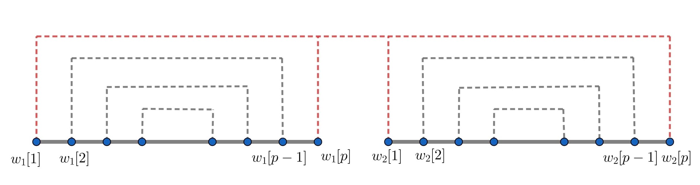
Figure 1. A pictorial representation of a sentence $W=(w_{1},w_{2})$ obeying (3.4)

Let $n\in\mathbb{N}$ and $p$ even be fixed. Since $\mathcal{S}_{n}$ is non-empty, there exist some row $R_{i}$ such that $\mathcal{S}_{n}\cap R_{i}$ is non-empty. It follows from condition $(ii)$ that $\#\{\mathcal{S}_{n}\cap R_{i}\neq\phi\}\geq c_{2}N$ and since $\mathcal{S}_{n}=\mathcal{S}_{n}^{T}$, $\#\{j:\mathcal{S}_{n}\cap R_{j}\neq\phi\}\geq c_{2}N$. Choose $\pi_{1}(0)$ from the set $\{j:\mathcal{S}_{n}\cap R_{j}\neq\phi\}$ and therefore the number of choices for $\pi_{1}(0)$ is at least $c_{2}N$. Since $\mathcal{S}_{n}\cap R_{\pi_{1}(0)}$ is non-empty, $\mathcal{S}_{n}\cap R_{\pi_{1}(0)}$ has at least $c_{2}N$ elements. Choose $\pi_{1}(1)$ from the set, so that $\left(\pi_{1}(0),\pi_{1}(1)\right)\in\mathcal{S}_{n}$.

For $1\leq i\leq p/2$, suppose $\pi_{1}(0),\pi_{1}(1),\ldots,\pi_{1}(i-1)$ are chosen such that $\left(\pi_{1}(j-1),\pi_{1}(j)\right)\in\mathcal{S}_{n}$ for all $1\leq j\leq i-1$. Since $\left(\pi_{1}(i-2),\pi_{1}(i-1)\right)\in\mathcal{S}_{n}$ and $\mathcal{S}_{n}=\mathcal{S}_{n}^{T}$, we get $\mathcal{S}_{n}\cap R_{\pi_{1}(i-1)}$ is non-empty and we choose $\pi_{1}(i)$ such that $\left(\pi_{1}(i-1),\pi_{1}(i)\right)\in\mathcal{S}_{n}$. Then the number of choices for $\pi_{1}(i)$ is bounded below by $c_{2}N$. For $p/2+1\leq i\leq p$, we define $\pi_{1}(i)=\pi_{1}(p-i)$. Then it follows that for $p/2+1\leq i\leq p$,

$$w_{1}[i] =L_{n}\left(\pi_{1}(i-1),\pi(i)\right)$$

$$=L_{n}\left(\pi_{1}(p-i+1),\pi_{1}(p-i)\right)$$

$$=L_{n}\left(\pi_{1}(p-i),\pi_{1}(p-i+1)\right)$$

$$=w_{1}[p-i+1].$$

Furthermore, $\pi_{1}(p)=\pi_{1}(0)$ and since $A_{n}$ is symmetric, $(\pi_{1}(p-i+1),\pi_{1}(p-i))\in\Delta_{n}$ for all $p/2+1\leq i\leq p$. Therefore by construction, $\pi_{1}\in\Pi_{L_{n},\Delta_{n}}^{*}(w_{1})$ and the number of choices of $\pi_{1}$ is bounded below by $(c_{2}N)^{p/2+1}$.

Next, we calculate the number of choices of $\pi_{2}$ such that $(\pi_{1},\pi_{2})\in\Pi_{L_{n},\Delta_{n}}^{*}(W)$. As we have already chosen $\pi_{1}$, we have that $w_{2}[1]=L_{n}\left(\pi_{1}(0),\pi_{1}(1)\right)=r_{u}$ is already fixed. Choose $\pi_{2}(0)$ such that $(\pi_{2}(0),j)\in\mathcal{S}_{n}$ and $L_{n}(\pi_{2}(0),j)=r_{u}$ for some $j$. By condition $(i)$, the number of choices for $\pi_{2}(0)$ is bounded below by $c_{1}N/B$. We choose $\pi_{2}(1)$ such that $L_{n}(\pi_{2}(0),\pi_{2}(1))=r_{u}$. Note that such a choice for $\pi_{2}(1)$ always exist.

For $2\leq i\leq p/2$, the letter $w_{2}[i]$ has not yet appeared. Suppose $\pi_{2}(0),\pi_{2}(1),\ldots,\pi_{2}(i-1)$ are chosen such that $\left(\pi_{2}(j-1),\pi_{2}(j)\right)\in\mathcal{S}_{n}$ for all $1\leq j\leq i-1$. Then the number of choices of $\pi_{2}(i)$ such that $\left(\pi_{2}(i-1),\pi_{2}(i)\right)\in\mathcal{S}_{n}$ is bounded below by $c_{2}N$. For $p/2+1\leq i\leq p$, we define $\pi_{2}[i]=\pi_{2}[p-i]$. Therefore the number of choices for $\pi_{2}$ is bounded below by $c_{1}N(c_{2}N)^{p/2-1}/B$. It then follows that $\pi_{2}$ is a circuit and $(\pi_{1},\pi_{2})\in\Pi_{L_{n},\Delta_{n}}^{*}(W)$. Hence, $\#\Pi_{L_{n},\Delta_{n}}^{*}(W)\geq(c_{2}N)^{p/2+1}\times\frac{c_{1}N}{B}(c_{2}N)^{p/2-1}$. As a result, we get

$$\sigma_{p}^{2}\geq\lim_{n\rightarrow\infty}\frac{1}{N^{p+1}}\#\Pi_{L_{n},\Delta_{n}}^{*}(W)\geq\lim_{n\rightarrow\infty}\frac{1}{N^{p+1}}\frac{c_{1}N}{B}(c_{2}N)^{p}=\frac{c_{1}c_{2}^{p}}{B}>0.$$

This completes the proof of theorem. ∎

4. Proofs of Propositions 22 and 24

First we develop and introduce some concepts and notions which will appear throughout the proofs of the propositions.

4.1. Generating vertices:

In this section, we introduce the concept of generating vertices and the role they would play in the calculations. First we give a definition of generating vertices. This is a more general version of the concept of generating vertices in [16].

Definition 26.

(a) For a sentence $W\in\mathcal{W}_{p,k}$, any combination $(u,j)$ where $1\leq u\leq k$ and $0\leq j\leq p$ is called a vertex. (b) For a sentence $W=(w_{1},w_{2},\ldots,w_{k})\in\mathcal{W}_{p,k}$, a set $A\subset S_{W}$ and a total ordering $`<$’ on $\{(u,j):1\leq u\leq k,0\leq j\leq p\}$, a vertex $(u,j)$ called a generating vertex of $W$ if

1. $j=0$ or

2. $w_{u}[j]\notin A$, $w_{\ell}[i]\neq w_{u}[j]$ for all $(\ell,i)<(u,j)$.

Note that generating vertices depend on the set $A$ and the ordering $<$. If $A$ is not specified, we choose $A$ as the empty set and $<$ as the dictionary order on $\{(u,j):1\leq u\leq k,0\leq j\leq p\}.$ Recall the graph $G_{W}=(V_{W},E_{W});W\in\mathcal{W}_{p,k}$, defined in Definition 9.

Another ordering we shall consider is the following: Consider a bijection $\zeta:V_{W}\rightarrow[k]$. The map $\zeta$ is called a renumbering of vertices in connection with Definition 9. We define an ordering with respect to $\zeta$ by $(\ell,i)<(u,j)$ if $(\zeta^{-1}\ell,i)$ is less than $(\zeta^{-1}u,j)$ under the dictionary ordering.

Note that for a sentence $W$ and a set $A\subset S_{W}$, the number of generating vertices does not depend on the ordering, and we denote the number of generating vertices in $W$ by $F(W,A)$.

It follows immediately that for a sentence $W\in\mathcal{W}_{p,k}$ and $A=\phi$, the number of generating vertices in $W$ is $|W|+k$, where $|W|$ denotes the number of distinct letters in $S_{W}$. We explain the concept of generating vertex through the following example:

Example 27.

Consider the sentence $W=(abca,addc,aedc,ebbd)$. For $W$, the set of generating vertices is $\{(1,0),(1,1),(1,2),(1,3),(2,0),(2,2),(3,0),(3,2),(4,0)\}$.

Soon, we shall see that the concept of generating vertices play an important role in determining the cardinality of $\Pi_{L}(W)$. In this regard, the introduction of vertices such that $j=0$ is intuitive as for each word $w_{i}$, a circuit is a map from $\{0,1,2,\ldots,p\}$ and to count the number of different possibilities of circuits $\pi_{i}$, $\pi_{i}(0)$ also needs to be determined. We first present an example that contains important ideas required to determine cardinality of $\Pi_{L}^{*}(W)$.

Example 28.

Consider the word $w=abab$ and let $L:[N]\rightarrow\mathbb{Z}^{d}$ be a link function obeying Assumption IV. Considering $w$ as a sentence in $\mathcal{W}_{p,1}$, the set of generating vertices of $w$ is $\{(1,0),(1,1),(1,2)\}$.

To find the cardinality of $\Pi_{L}^{*}(w)$, we start counting the possible values of $\pi(i)$ starting from $\pi(0)$ for circuits $\pi\in\Pi_{L}^{*}(w)$. As there are no constraints on the value of $\pi(0)$, the number of possible choices for $\pi(0)$ is $N$. Similarly, the number of choices for $\pi(1)$ and $\pi(2)$ are also $N$, as there are no constraints for $\pi(1)$ and $\pi(2)$. Once $\pi(0)$ and $\pi(1)$ are chosen, the condition $w[1]=w[3]$ dictates that $L(\pi(2),\pi(3))$ should be equal to $L(\pi(0),\pi(1))$ which is already fixed. Since $L$ obeys Assumption IV, the maximum number of possibilities for $\pi(3)$ is bounded by $B$. As $\pi(4)=\pi(0)$, the value of $\pi(4)$ is already determined. Thus we obtain the following bound for the cardinality of $\Pi_{L}^{*}(w)$:

$$\#\Pi_{L}^{*}(w)\leq N\times N\times N\times B\times 1=O(N^{|F|}),$$

where $F$ is the number of generating vertices in $W$. Intuition should suggest that the same upper bound would hold for any sentence $W$.

Now, we present another example and show that the above bound is not tight and the upper bound can be reduced by an order of $N$.

Example 29.

Consider the word $w=abacb$. Note that the letter $w[4]=c$ appears only once in $w$. We shall exploit this property to show that $\#\Pi_{L}^{*}(w)\leq O(N^{F-1})$.

We start by counting the number of choices for $\pi(0)$ and proceed in increasing order to assign values till $\pi(3)$. From Example 28 it is clear that the number of choices for $\pi(0),\pi(1),\pi(2),\pi(3)$ is $N^{3}\times B$. Now we move to the end, and assign value to $\pi(5)$. As $\pi(5)=\pi(0)$, there is only one choice for $\pi(5)$. Further, note that $L(\pi(4),\pi(5))=L(\pi(1),\pi(2))$ and the latter quantity is already fixed. Therefore, from Assumption IV, the number of choices for $\pi(4)$ is bounded above by $B$. Hence

$$\#\Pi_{L}^{*}(w)\leq N^{3}B\times B\times 1=O(N^{F-1}).$$

In the next lemma, we extend the reasoning in above examples for arbitrary sentences.

Lemma 30.

Let $L:[N]\rightarrow\mathbb{Z}^{d}$ be a link function obeying Assumption IV. For $k\in\mathbb{Z}_{+}$ and $W\in\mathcal{W}_{p,k}$, let $\pi_{1},\pi_{2},\ldots,\pi_{t-1}:\{0,1,2,\ldots,p\}\rightarrow[N]$ be circuits such that $(\pi_{1},\pi_{2},\ldots,\pi_{t-1})\in\Pi_{L}^{*}(w_{1},w_{2},\ldots,w_{t-1})$. Suppose $Q_{t}=\#\{\pi_{t}:(\pi_{1},\pi_{2},\ldots,\pi_{t})\in\Pi_{L}^{*}(w_{1},w_{2},\ldots,w_{t})\}$. Then

$$Q_{t}\leq\begin{cases}B^{p+1}N^{F_{t}-1}&\text{ if }\exists\ a\in S_{w_{t}}\text{ such that }m_{S_{w_{t}}}(a)=1\text{ and }m_{S_{w_{\ell}}}(a)=0\text{ for all }\ell<t,\\ B^{p+1}N^{F_{t}}&\text{ otherwise},\end{cases}$$

where $F_{t}$ is the number of generating vertices in $w_{t}$.

Proof.

We first consider the case where $S_{w_{t}}$ does not contain any letter that is repeated only once in $S_{w_{t}}$. We start by assigning values for $\pi_{t}(0)$ and proceed in ascending order till $\pi_{t}(p)$. Note that the number of possibilities of $\pi_{t}(0)$ is $N$. Further, by the logic followed in Example 28 it is clear that if $w_{t}[j]$ is the first appearance of a letter in the sentence $W$, then there is no prior constraint involving $L(\pi_{t}(j-1),\pi_{t}(j))$, and therefore the number of choices for $\pi_{t}(j)$ is $N$. Further if the letter $w_{t}[j]$ has already appeared, then note that the numerical value $L(\pi_{t}(j-1),\pi_{t}(j))$ is already determined by the choice of $\pi_{1},\pi_{2},\ldots,\pi_{t-1}$ and $\pi_{t}(0),\pi_{t}(1),\ldots,\pi_{t}(j-1)$. Therefore, due to Assumption IV, the number of values for $\pi_{t}(j)$ is bounded above by $B$. It follows from here that

$$Q_{t} \leq N^{F_{t}}B^{(p+1)-F_{t}}\leq N^{F_{t}}B^{p+1}.$$

Now suppose $S_{w_{t}}$ contains a new letter that is repeated only once in $S_{w_{t}}$. Let $a=w_{t}[i]$ be the last letter such that $a\notin S_{w_{\ell}}$ for all $\ell<t$ and $m_{S_{w_{t}}}(a)=1$.

We count the number of choices for $\pi_{t}$ in the following way: We start by counting the number of choices for $\pi_{t}(0)$. Note that $\pi_{t}(0)$ has $N$ choices. For $j<i$, suppose the value of $\pi_{t}(0),\pi_{t}(1),\ldots,\pi_{t}(j-1)$ are chosen. If $(t,j)$ is a generating vertex, then note that the value of $L(\pi_{t}(j-1),\pi_{t}(j))$ is not fixed and therefore the number of choices for $\pi_{t}(j)$ is $N$. If $(t,j)$ is not a generating vertex, then by Assumption IV, the number of choices for $\pi_{t}(j)$ is bounded above by $B$.

Once all $\pi_{t}(j)$ till $j\leq i-1$ are determined, we start assigning values to $\pi_{t}(j)$ starting from $\pi_{t}(p)$ and proceeding in the decreasing order of $j$ till $\pi_{t}(i)$. Note that the number of choices for $\pi_{t}(p)$ is 1, as $\pi_{t}(p)=\pi_{t}(0)$. Suppose $\pi_{t}(p),\pi_{t}(p-1),\ldots,\pi_{t}(p-j+1)$ are chosen for some $0\leq j\leq p-i$ and the letter $w_{t}[p-j+1]$ is not appeared yet. Then it follows that the value of $L(\pi_{t}(p-j),\pi_{t}(p-j+1))$ is not fixed and therefore $\pi_{t}(p-j)$ has $N$ choices. And like in the previous case, if the letter $w_{t}[p-j+1]$ has already appeared, then the value of $L(\pi_{t}(p-j),\pi_{t}(p-j+1))$ is already fixed and therefore due to Assumption IV, $\pi_{t}(p-j)$ has at most $B$ choices. As a result, the value of $\pi_{t}(i)$ is determined by the value of other $\pi_{t}(j)$, even though $(t,i)$ is a generating vertex. Note that by this construction, for all generating vertices other than $(t,i)$, there exist a component ($\pi_{t}(j)$ or $\pi_{t}(j-1)$ depending on whether $j<i$ or $j>i$) which has $N$ choices and the number of choices for all other $\pi_{t}(j)$ is bounded above by $B$. Hence, $Q_{t}$ is bounded above by $B^{p+1}N^{F_{t}-1}$. This completes the proof. ∎

Recall the notion of renumbering of vertices and ordering with respect to renumbering from Definition 26. The following lemma is an immediate generalization of Proposition 24 and would follow from a similar argument.

Lemma 31.

Let $L:[N]\rightarrow\mathbb{Z}^{d}$ be a link function obeying Assumption IV. For $k\in\mathbb{Z}_{+}$ and $W\in\mathcal{W}_{p,k}$, let $\zeta:V_{W}\rightarrow[k]$ be a bijection and let $\pi_{\zeta^{-1}(1)},\pi_{\zeta^{-1}(2)},\ldots,\pi_{\zeta^{-1}(t-1)}:\{0,1,2,\ldots,p\}\rightarrow[N]$ be circuits such that $(\pi_{\zeta^{-1}(1)},\pi_{\zeta^{-1}(2)},\ldots,\pi_{\zeta^{-1}(t-1)})\in\Pi_{L}^{*}(w_{\zeta^{-1}(1)},w_{\zeta^{-1}(2)},\ldots,w_{\zeta^{-1}(t-1)})$. Suppose $Q_{t}=\#\{\pi_{\zeta^{-1}(t)}:(\pi_{\zeta^{-1}(1)},\pi_{\zeta^{-1}(2)},\ldots,\pi_{\zeta^{-1}(t)})\in\Pi_{L}^{*}(w_{\zeta^{-1}(1)},w_{\zeta^{-1}(2)},\ldots,w_{\zeta^{-1}(t)})\}$. Then

$$Q_{t}\leq\begin{cases}B^{p+1}N^{F_{\zeta^{-1}(t)}-1}&\text{ if }\exists\ a\in S_{w_{t}}\text{ such that }m_{S_{w_{\zeta^{-1}(t)}}}(a)=1,m_{S_{w_{\zeta^{-1}(\ell)}}}(a)=0\text{ for all }\ell<t,\\ B^{p+1}\left(N^{F_{\zeta^{-1}(t)}}\right)&\text{ otherwise},\end{cases}$$

where $F_{\zeta^{-1}(t)}$ is the number of generating vertices in $w_{\zeta^{-1}(t)}$.

4.2. Proof of Propositions 22:

We prove Proposition 22 for parts (a) and (b) separately. First, we prove part (a).

Proof of Proposition 22 (a).

First consider $W=(w_{1},w_{2})\in\mathcal{P}_{2}(p,p)$. Let $a\in S_{w_{1}}\cap S_{w_{2}}$ be a cross-matched letter. Note that $a$ appears only once in $S_{w_{1}}$ and thus by Lemma 30, it follows that the number of choices for $\pi_{1}=O(N^{F_{1}-1})$, where $F_{1}$ is the number of generating vertices in $S_{w_{1}}$. Similarly, the number of choices for $\pi_{2}$ is $O(n^{F_{2}})$, where $F_{2}$ is the number of generating vertices in $S_{w_{2}}$. Thus we get

$$\frac{1}{N^{p+1}}\#\Pi_{L_{n}}^{*}(W)=\frac{1}{N^{p+1}}O(N^{F_{1}+F_{2}-1})=O(1).$$

Here the last equality in the above expression follows from the fact that $F_{1}+F_{2}=|W|+1$, where $|W|$ is the total number of letters in $S_{W}$, which is $p$.

Now for $W=(w_{1},w_{2})\in\mathcal{P}_{2,4}(p,p)$, note that each letter in $S_{w_{i}}$ is repeated exactly twice in $S_{w_{i}}$ and therefore from Lemma 30, we get that, the number of choices for $\pi_{1}$ is $O(N^{F_{1}})$ and the number of choices for $\pi_{2}$ is $O(N^{F_{2}})$. Thus, it follows that for all $W\in{\mathcal{P}}_{2,4}(p,p)$,

$$\frac{1}{N^{p+1}}\#\Pi_{L_{n}}^{*}(W)=\frac{1}{N^{p+1}}O(N^{F_{1}+F_{2}})=O(1),$$

where the last equality follows as the number of distinct letters in $S_{W}$ is $(p-1)$.

Next, consider $W=(w_{1},w_{2})\in\mathcal{W}_{p,2}\setminus{\mathcal{P}}_{2}(p,p)$ with at least one cross-matched letter and each letter in $S_{W}$ appearing at least twice. Suppose $\#\Pi_{L_{n}}(W)\geq cN^{p+1}$ for some $c>0$. We shall show that this happens only if $W\in\mathcal{P}_{2,4}(p,p)$.

Since each letter in $S_{W}$ is repeated at least twice, $|W|\leq p$, where $|W|$ is the number of distinct letters in $S_{W}$. It follows from Lemma 30 that the number of elements in $\Pi_{L_{n}}^{*}(W)$ is at most $O(N^{|W|+2})$. Thus $\#\Pi_{L_{n}}^{*}(W)\geq cN^{p+1}$ only if $|W|\geq p-1$. Hence, the only possibilities are $|W|\in\{p-1,p\}$.

Suppose $|W|=p$, then since each letter in $S_{W}$ appears at least twice and the condition that $W$ has at least one cross-matched element implies that $W\in\mathcal{P}_{2,2}(p,p)$, a contradiction.

Now, let $|W|=p-1$. Suppose there exists an element $a\in S_{w_{i}}$ such that $a$ is repeated only once in $S_{w_{i}}$ for $i=1$ or $2$. Then from Lemma 30, the number of choices for $\pi_{i}$ is $O(N^{F_{i}-1})$ and consequently, $\#\Pi_{L_{n}}^{*}(W)=O(N^{|W|+1})=O(N^{p})$. Thus, for $\#\Pi_{L_{n}}^{*}(W)$ to be the order $O(N^{p+1})$, each cross-matched element must be repeated at least four times, twice in both $S_{w_{1}}$ and $S_{w_{2}}$. Let $r$ be the number of cross-matched elements in $W$. Then we have

$$4r+2(p-1-r)\leq 2p\implies r=1.$$

This implies that $W\in\mathcal{P}_{2,4}(p,p)$. To prove the rest, note that for any sentence $W\in{\mathcal{P}}_{2}(p,p)\cup{\mathcal{P}}_{2,4}(p,p)$, the set $\Pi_{L_{n},\Delta_{n}}^{*}(W)\setminus\Pi_{L_{n},\Delta_{n}}(W)$ can be written as a union of sentences belonging to $\mathcal{W}_{p,k}$, with number of letters is strictly less than the number of letters of $W$. As a result, it follows that

$$\frac{1}{N^{p+1}}\#\Pi_{L_{n}}(W)\leq\frac{1}{N^{p+1}}\#\Pi_{L_{n}}^{*}(W),$$

and this completes the proof for part (a). ∎

Proof of Proposition 22 (b).

Let $W=(w_{1},w_{2},\ldots,w_{k})\in\mathcal{W}_{p,k}$ be a clique sentence with the letter $a\in S_{W}$ repeating exactly $k$ times. Then the number of distinct letters in $W$ is $|W|=\frac{pk-k}{2}+1$. From the definition of clique sentence it follows that $a$ appears only once in $w_{1}$ and therefore by an application of Lemma 30, the cardinality of $\Pi_{L}^{*}(W)$ is bounded above by $O(N^{|W|+k-1})$. Therefore,

$$\frac{1}{N^{\frac{pk+k}{2}}}\#\Pi_{L}^{*}(W)\leq\frac{1}{N^{\frac{pk+k}{2}}}O(N^{|W|+k-1})=O(1).$$

Since $\#\Pi_{L}(W)\leq\#\Pi_{L}^{*}(W)$, the proof follows. ∎

4.3. Proof of Proposition 24:

Observe from the discussions in Section 3.1 that Proposition 24 is the heart of this paper. Now we proceed to prove it.

Recall from Lemma 30 that for a sentence $W=(w_{1},w_{2},\ldots,w_{k})$, if $\pi_{1},\pi_{2},\ldots,\pi_{t-1}$ are chosen, then the number of choices for $\pi_{t}$ is at most $O(N^{F_{t}})$, where $F_{t}$ is the number of new letters in $w_{t}$. Since $\mathbb{E}x_{i}=0$, it follows from standard calculations that for non-zero expectation, each letter must appear at least twice in $S_{W}$. Thus, we focus on sentences of that form and for such sentence, the number of letters is at most $pk/2$. As a result, we get that the maximum order of $\#\Pi_{L}^{*}(W)=O(N^{\frac{pk}{2}+k})$.

For a sentence $W$ such that each letter appears at least twice, and $G_{W}$ is connected, $G_{W}$ has at least $k-1$ edges. Consider an edge $\{i,j\}\in E_{W}$ and a cross-matched letter, say ‘$a$’, belonging to $S_{w_{i}}\cap S_{w_{j}}$. Lemma 30 says that if ‘$a$’ is a new letter that appears only once, then the degree of freedom for choosing $\pi_{t}$ reduces by $1$. Otherwise, $a$ must appear at least thrice in $S_{W}$, in vague terms, leading to a loss of half a degree of freedom. Thus, even in the worst case, there is a loss of $(k-1)/2$ degrees of freedom. We shall prove Proposition 24 by showing that there is a loss of at least $(k+1)/2$ degrees of freedom whenever $W$ is not a clique sentence.

Outline of the proof: For better readability, we divide the proof of Proposition 24 to three steps as given below. Step I: The discussion in the starting of this subsection highlights the role of cross-matching letters in proving Proposition 24. With this cue, we first consider one of the simplest cases possible, where there is a choice of distinct cross-matched letters for each edge.

Definition 32.

For $k\geq 3,p\geq 1$, consider a sentence $W\in\mathcal{W}_{p,k}$ such that $G_{W}$ is connected. We say $W\in\mathcal{C}_{p,k}$ if $G_{W}$ has a spanning tree $T_{W}$ and there exist a function $\varphi:E(T_{W})\rightarrow S_{W}$ such that

1. $\varphi$ is a one-one function where for all $\{i,j\}\in E(T_{W})$, $\varphi(\{i,j\})\in S_{w_{i}}\cap S_{w_{j}}$, and

2. each letter in $S_{W}$ appears at least twice in $S_{W}$.

We first show that for each $W\in\mathcal{C}_{p,k}$, (17) holds (see Lemma 34). This is obtained by choosing a reordering of vertices such that there is maximum loss of degree of freedom.

Step II: For $W\in\mathcal{W}_{p,k}$, we consider a particular type of subgraph $H_{W}$ of $G_{W}$, which corresponds to the case where each connected component of $H_{W}$ is a tree $T_{W}$ with properties considered in Definition 32, along with some additional conditions.

Definition 33.

For a sentence $W=(w_{1},w_{2},\ldots,w_{k})\in\mathcal{W}_{p,k}$ with $m_{S_{W}}(a)\geq 2$ for all $a\in S_{W}$, a subgraph $H_{W}\subset G_{W}$ with connected components $T_{1},T_{2},\ldots,T_{r}$ is called a Type I subgraph, if

1. $V(H_{W})=\{1,2,\ldots,k\}$ and $H_{W}$ is a forest,

2. $\#V(T_{1})\geq 3$ and if $\#V(T_{j})=1$ for some $j$, then $\#V(T_{i})=1$ for all $i>j$,

3. For all $a\in S_{W_{T_{m}}}$, $1\leq m\leq r$, $a$ appears at least twice in $\bigcup_{i\leq m}S_{W_{T_{i}}}$, and

4. there exists a one-one map $\varphi:E(H_{W})\rightarrow S_{W}$ such that $\varphi(\{i,j\})\in S_{w_{i}}\cap S_{w_{j}}$ for each $\{i,j\}\in E(H_{W})$.

Pictorially, Type I subgraph can be represented as seen in Figure 2.

Figure 2. Example of a Type I subgraph with $a_{e}=\varphi(e)$ as distinct letters.

In Lemma 38 , we show that any $W\in\mathcal{W}_{p,k};k\geq 3$ such that $G_{W}$ is connected and not a special cluster, has a Type I subgraph. Step III: Finally, to prove Proposition 24, we show that if a sentence $W$ has a Type I subgraph, then

$$\frac{1}{N^{\frac{pk+k}{2}}}\#\Pi_{L_{n}}^{*}(W)=o(1).$$

Combining it with Step II implies Proposition 24. Now, we move on to the detailed proof: Step I: Before proceeding to this step in detail, we recall the following terminology from graph theory. For a finite graph $G=(V,E)$, and a vertex $v\in V$, the eccentricity of $v$ is defined as $g[v]=\sup\{\operatorname{dist}(i,v):i\in V\}$, where $\operatorname{dist}(i,v)$ is the length of the shortest path from $i$ to $v$ through the edges of $G$. The center of $G$ is defined as the set $\mathbb{O}(G)=\{v\in V:g[v]\leq g[i]\,\,\forall\ i\in V\}$. For a tree $T$, it is known that $\#\mathbb{O}(T)\leq 2$ and if $T$ has more than two vertices, then for each $o\in\mathbb{O}(T)$, $\operatorname{deg}(o)\geq 2$. Recall the notion of renumbering of vertices in Definition 26. Let $W\in\mathcal{C}_{p,k}$ such that $T_{W}$ is a spanning tree of $G_{W}$, $\varphi:E(T_{W})\rightarrow S_{W}$ is a one-one map obeying condition (i) of Definition 32, and let $\zeta$ be a renumbering of vertices obeying the following condition:

$$\operatorname{dist}\left(\mathbb{O}(T_{W}),j\right)<\operatorname{dist}\left(\mathbb{O}(T_{W}),i\right)\implies\zeta(i)<\zeta(j).$$ (24)

Recall the multi-set $S_{W}$ defined in Definition 6 and let $m_{S_{W}}$ and $m_{S_{w_{i}}}$ be the multiplicity function for $S_{W}$ and $S_{w_{i}}$, respectively. We also fix the convention that for an edge $\{i,j\}\in E(T_{W})$, we define

$$a_{i,j}:=\varphi(\{i,j\})\text{ where }\zeta(i)<\zeta(j).$$ (25)

Note that in the definition of $a_{i,j}$ the ordering of $i,j$ is important and this distinction will play an important role in the proofs later. We remark that for any finite graph $G$, there always exists a renumbering $\zeta$ of vertices obeying (24).

For a set $A\subset S_{W}$, consider the following sets:

$$\mathcal{C}_{A}=\{a_{i,j}:a_{i,j}\notin S_{w_{\ell}}\,\,\forall\ \zeta(\ell)<\zeta(i),a_{i,j}\notin A\text{ and }m_{S_{w_{i}}}(a_{i,j})=1\},$$

$$\widetilde{\mathcal{C}}_{A}=\operatorname{Im}(\varphi)\setminus\mathcal{C}_{A}.$$ (26)

Note that the sets $\mathcal{C}_{A}$ and $\widetilde{\mathcal{C}}_{A}$ depend on the renumbering $\zeta$, but we are suppressing $\zeta$ for notational convenience. From the definition of $\widetilde{\mathcal{C}}_{A}$, it follows that each letter $a_{i,j}\in\widetilde{\mathcal{C}}_{A}$ such that $a_{i,j}\notin A$ appears at least thrice in $S_{W}$.

The following lemma provides the contribution of the sentences in $\mathcal{C}_{p,k}$ for $k\geq 3$, where $\mathcal{C}_{p,k}$ as in Definition 32.

Lemma 34.

For $p\geq 1,k\geq 3$, let $W\in\mathcal{C}_{p,k}$ and $\{L_{n}\}$ be a sequence of link functions obeying Assumption IV. Then

$$\frac{1}{N^{\frac{pk+k}{2}}}\#\Pi^{*}_{L_{n}}(W)=o(1).$$

We first state a lemma required in the proof of Lemma 34.

Lemma 35.

For $k\geq 3$ and $p\geq 1$, let $W\in\mathcal{W}_{p,k}$ be such that $G_{W}$ is connected. Suppose $T_{W}$ is a spanning tree of $G_{W}$, $\varphi:E(T_{W})\rightarrow S_{W}$ is a one-one function, $\zeta$ is a renumbering obeying (24), $\{L_{n}\}$ is a sequence of link functions obeying Assumption IV and $A\subset S_{W}$. Then

$$\#\Pi_{L_{n}}^{*}(W)=O(N^{F-R}),$$ (27)

where for a given $A$, $F=F(W,A)$ is the number of generating vertices of $W$ given A, defined in Definition 26 and $R=\#\mathcal{C}_{A}$.

Assuming Lemma 35, we now prove Lemma 34. The proof of Lemma 35 is given later.

Proof of Lemma 34.

Recall the definition of $\mathcal{C}_{A}$ from (4.3). In this proof, we choose $A$ as the null set, and denote $\mathcal{C}=\mathcal{C}_{\phi}$ and $\widetilde{\mathcal{C}}=\widetilde{\mathcal{C}}_{\phi}$. We prove the proposition by dividing into cases based on different values for $R=\#\mathcal{C}$.

Case 1: $R\geq 2$ for some choice of renumbering $\zeta$ obeying $(\ref{eqn: condition zeta})$.

Fix a renumbering $\zeta$ obeying (24) such that $R\geq 2$. First note that each element of $\widetilde{\mathcal{C}}$ appears at least thrice in $S_{W}$ and each element in $\mathcal{C}$ appears at least twice. Considering the fact that every element in $S_{W}$ also appears at least twice, we get that the number of elements in the multi-set $S_{W}\setminus\operatorname{Im}(\varphi)$ is at most $\frac{pk-3(k-1-R)-2R}{2}$. Clearly, the number of elements in $\operatorname{Im}(\varphi)$ is $k-1$. As a result, we get that the number of generating vertices of $W$ is

$$F=|W|+k\leq\frac{pk-3(k-1-R)-2R}{2}+(k-1)+k=\frac{pk}{2}+\frac{k}{2}+\frac{1+R}{2}.$$

Thus, it follows from Lemma 35 that $\frac{1}{N^{\frac{pk+k}{2}}}\#\Pi_{L_{n}}^{*}(W)=O(N^{\frac{1-R}{2}})=o(1)$ if $R\geq 2$. Before going to the next case, we define another quantity. Let

$$\mathcal{D}=\{a_{i,j}\in\widetilde{\mathcal{C}}:m_{S_{W}}(a_{i,j})\geq 4\}\text{ and }U=\#\mathcal{D}.$$ (28)

Note that $\mathcal{D}$ and $U$ depends on the sentence $W$, the map $\varphi$ and the renumbering $\zeta$. Case 2: $R=0$ for some choice of renumbering $\zeta$ obeying $(\ref{eqn: condition zeta})$.

Let $\zeta$ be a renumbering of vertices obeying $(\ref{eqn: condition zeta})$ such that $R=0$. We first consider the case $U\geq 2$, where $U$ is as defined in (28). Since $R=0$, by Lemma 35, we have $\#\Pi_{L_{n}}^{*}(W)=O(N^{F})$. Note that each letter in $\mathcal{D}$ appears at least four times, each letter in $\mathcal{C}$ appears at least thrice, and all other letters appear at least twice. Therefore,

$$F\leq\frac{pk-4U-3(k-1-U)}{2}+(k-1)+k=\frac{pk}{2}+\frac{k}{2}-\frac{U}{2}+\frac{1}{2}.$$

As a result, we get that $\frac{1}{N^{\frac{pk+k}{2}}}\#\Pi_{L_{n}}^{*}(W)=o(1)$ if $U\geq 2$.

Next consider the case $U\in\{0,1\}$. As $k\geq 3$, $T_{W}$ has at least two leaves. Since $U\leq 1$, there exists a leaf $i$ such that $\{i,j\}\in E(T_{W})$ and $m_{S_{W}}(a_{i,j})\leq 3$. Note that since $R=0$, $a_{i,j}\in\widetilde{\mathcal{C}}$ and therefore $m_{S_{W}}(a_{i,j})=3$.

To determine $\#\Pi_{L_{n}}^{*}(W)$, we consider a new reordering of vertices such that the first vertex is $j$. We start by counting the number of possible choices for the circuit $\pi_{j}$. Since $a_{i,j}\in\widetilde{\mathcal{C}}$, by construction of $\widetilde{\mathcal{C}}$ it follows that $m_{S_{w_{j}}}(a_{i,j})=1.$ Therefore, the number of choice for $\pi_{j}$ is $O(N^{F_{j}-1})$, where $F_{j}$ is the number of generating vertices of $w_{j}$. For the rest of the circuits $\pi_{r}$, the maximum number of possibilities of $\pi_{r}$ is $O(N^{F_{r}})$, where $F_{r}$ is the number of generating vertices of $w_{r}$ with respect to the new ordering. Therefore we get that $\#\Pi_{L_{n}}^{*}(W)=O(N^{|W|+k-1})$ and

$$|W|+(k-1)\leq\frac{pk-3(k-1)}{2}+(k-1)+(k-1)=\frac{pk+k-1}{2}.$$

Hence $\frac{1}{N^{\frac{pk+k}{2}}}\#\Pi_{L_{n}}^{*}(W)=O(N^{-1/2})=o(1)$. Now, we are left with only the following case: Case 3: $R=1$ for all choice of renumbering $\zeta$ obeying (24).

We fix a renumbering $\zeta$ obeying (24). Suppose $U\geq 1$, then by Lemma 35, the cardinality of $\Pi_{L_{n}}^{*}(W)=O(N^{F-R})=O(N^{F-1})$. Also, we get

$$F-1=|W|+k-1\leq\frac{pk-4U-3(k-2-U)-2}{2}+(k-1)+k-1=\frac{pk}{2}+\frac{k}{2}-\frac{U}{2}.$$

As a result, $\frac{1}{N^{\frac{pk+k}{2}}}\#\Pi_{L_{n}}^{*}(W)=O(N^{-U/2})=o(1),$ for all $U\geq 1$.

Now suppose $U=0$. Since $R=1$, there exists an edge $\{i,j\}\in E(T_{W})$ with $\zeta(i)<\zeta(j)$, such that $a_{i,j}\in\mathcal{C}$. We fix the edge $\{i,j\}$ for the rest of the proof. Suppose $m_{S_{W}}(a_{i,j})\geq 3$. Then we have $F-R\leq\frac{pk-3(k-1)}{2}+(k-1)+k-1$, and thus $\frac{1}{N^{\frac{pk+k}{2}}}\#\Pi_{L_{n}}^{*}(W)=o(1)$.

Thus, it is sufficient to prove for the case where $m_{S_{W}}(a_{i,j})=2$. We state the following claim:

Claim A: There exist a leaf $i^{\prime}$ such that $\{i^{\prime},j^{\prime}\}\in E(T_{W})$, $i\neq i^{\prime},j^{\prime}$ and $\operatorname{dist}(i^{\prime},\mathbb{O}(T_{W}))=\max\{\operatorname{dist}(\mathbb{O}(T_{W}),v):v\in V_{W}\}$.

Consider $i^{\prime},j^{\prime}$ from the above claim. Since $m_{S_{W}}(a_{i,j})=2$, $a_{i,j}$ belongs to $\mathcal{C}$ for all choice of $\zeta$ obeying (24) and this implies $a_{i^{\prime},j^{\prime}}\in\widetilde{\mathcal{C}}$ for all choice of $\zeta$ obeying (24). Using Claim A, without loss of generality assume $\zeta(i^{\prime})=1$. Combining $\zeta(i^{\prime})=1$ with the deduction $a_{i^{\prime},j^{\prime}}\in\widetilde{\mathcal{C}}$ and $U=0$, we get $m_{S_{w_{i^{\prime}}}}(a_{i^{\prime},j^{\prime}})=2$ and $m_{S_{w_{j^{\prime}}}}(a_{i^{\prime},j^{\prime}})=1$.

We determine the cardinality of $\Pi_{L_{n}}^{*}(W)$ in the following way. We start by counting the number of choices for $\pi_{i}\in\Pi_{L_{n}}^{*}(w_{i})$. Since $m_{S_{w_{i}}}(a_{i,j})=1$, by Lemma 30, the number of choices for $\pi_{i}$ is $O(N^{F_{i}-1})$, where $F_{i}$ is the number of generating vertices of $w_{i}$. Next, we count the number of possibilities for $\pi_{j^{\prime}}$ such that $(\pi_{i},\pi_{j^{\prime}})\in\Pi_{L_{n}}^{*}(w_{i},w_{j^{\prime}})$. Since $i\neq i^{\prime},j^{\prime}$ and $m_{S_{W}}(a_{i^{\prime},j^{\prime}})=3$ with $m_{S_{w_{i^{\prime}}}}(a_{i^{\prime},j^{\prime}})=2$ and $m_{S_{w_{j^{\prime}}}}(a_{i^{\prime},j^{\prime}})=1$, it follows that $a_{i^{\prime},j^{\prime}}$ has not appeared in $w_{i}$. Thus, $a_{i^{\prime},j^{\prime}}$ is a new letter that appears only once in $w_{j^{\prime}}$. Hence by Lemma 30, the number of choices for $\pi_{j^{\prime}}$ is $O(N^{F_{j^{\prime}}-1})$, where $F_{j^{\prime}}$ is the number of generating vertices of $w_{j^{\prime}}$ with respect to the new ordering. For all other choices of $r$, the maximum number of possibilities for $\pi_{r}$ is at most of the order $O(N^{F_{r}})$, where $F_{r}$ is the number of generating vertices of $w_{r}$ with respect to the new ordering. Therefore, we get $\#\Pi_{L_{n}}^{*}(W)\leq O(N^{|W|+k-2})$. We also have the inequality

$$|W|+k-2\leq\frac{pk-3(k-2)-2}{2}+k-1+k-2=\frac{pk}{2}+\frac{k}{2}-1.$$

Hence, it follows that $\frac{1}{N^{\frac{pk+k}{2}}}\#\Pi_{L_{n}}^{*}(W)=o(1)$ and this completes the proof. ∎

Figure 3. (a) is an example of a sentence such that $R=0$ for all choice of $\zeta$ obeying (24) and (b) gives a sentence such that $R=1$ for all choice of $\zeta$ obeying (24). In both the figures, for an edge $e$, the letter $\varphi(e)$ is given in green along the edge.

Remark 36.

We remark that the cases 1 and 2 in the proof of Lemma 34 are not distinct. But, none of the above cases are also not subcases of any of the other cases. See Figure 3 for an example.

Remark 37.

In Lemma 34, the upper bound on $\#\Pi_{L_{n}}^{*}(W)$ is obtained by subtracting $R$ from the upper bound on the number of generating vertices in $W$, with respect to $A=\phi$. Suppose $A\subset S_{W}$ is non-empty and let $W\in\mathcal{W}_{p,k}$ such that $m_{S_{W}}(a)\geq 2$ for all $a\notin A$ and suppose there exists a spanning tree $T_{W}$ of $G_{W}$ and a one-one function $\varphi:E(T_{W})\rightarrow S_{W}$ obeying condition (i) of Definition 32. Then the upper bound on the number of generating vertices of $W$ in this case, is less than the case when $A=\phi$. Hence here also, $\frac{1}{N^{\frac{pk+k}{2}}}\#\Pi_{L_{n}}^{*}(W)=o(1)$ for all $k\geq 3$.

Figure 4. Trees such that the distance of all vertices from the center is one. (a) shows the case when the center consists of only one vertex and (b) shows the case when the center consists of two vertices.

Next we prove Lemma 35. The proof is by induction on $r=\max\{\operatorname{dist}\left(\mathbb{O}(T_{W}),v\right):v\in V_{W}\}$, where $\mathbb{O}(T_{W})$ is the center of $T_{W}$.

Proof of Lemma 35.

Let $r=\max\{\operatorname{dist}\left(\mathbb{O}(T_{W}),v\right):v\in V_{W}\}$ and let $A\subseteq S_{W}$. For $r=1$, $T_{W}$ is one of the forms given in Figure 4. First suppose that $T_{W}$ is a star graph considered in Figure 4 (a). Without loss of generality assume that $\zeta$ is the identity map on $[k]$. Then the image set of the map $\varphi$ is given by $\{a_{i,k}:1\leq i\leq k-1\}$, where $a_{i,k}$ is as defined in (25). Note that the number of choices for $\pi_{1}$ is $O(N^{F_{1}})$ if $a_{1,k}$ appears more than once in $S_{w_{1}}$ and is of the order $O(N^{F_{1}-1})$ if $a_{1,k}$ appears only once in $S_{w_{1}}$, where $F_{1}$ is the number of generating vertices of $w_{1}$ with respect to $\zeta$. For $2\leq i\leq k$, once $\pi_{1},\pi_{2},\ldots,\pi_{i-1}$ are chosen, the number of choices for $\pi_{i}$ is $O(N^{F_{i}-1})$ if $a_{i,k}\in\mathcal{C}_{A}$ and is of the order $O(N^{F_{i}})$ if $a_{i,k}\notin\mathcal{C}_{A}$, where $F_{i}$ is the number if generating vertices of $w_{i}$ with respect to $\zeta$. Now, for $T_{W}$ as the graph considered in Figure 4 (b), note that a similar argument again works. Combining the above observations, we get the result for $r=1$.

Now, we move to the induction step: Suppose the result holds for all sentences $W$ with a spanning tree $T_{W}$ such that $\max\{\operatorname{dist}\left(\mathbb{O}(T_{W}),v\right):v\in V_{W}\}\leq r\in\mathbb{N}$ and all choices of $A\subset S_{W}$. Let $W$ be a sentence with a spanning tree $T_{W}$ such that $\max\{\operatorname{dist}\left(\mathbb{O}(T_{W}),v\right):v\in V_{W}\}=(r+1)$ and assume without loss of generality that $\zeta$ is the identity map. Let $W^{\prime}$ be the sentence obtained from $W$ after the deletion of all words $w_{i}$ such that $\operatorname{dist}(i,\mathbb{O}(T_{W}))=r+1$ (see Figure 5). Consider the spanning tree $T_{W^{\prime}}$ of $G_{W^{\prime}}$ obtained by the restriction of $T_{W}$ to $V(G_{W^{\prime}})$ and define $\varphi^{\prime}=\varphi|_{E(W^{\prime})}$. Define $\zeta^{\prime}:V(G_{W^{\prime}})\rightarrow\{1,2,\ldots,k-q\}$ given by $\zeta^{\prime}(i):=\zeta(i)-q$, where $q$ is the number of vertices in $T_{W}$ at a distance of $r+1$ from the center of $T_{W}$. It follows that $\zeta^{\prime}$ is a bijection obeying (24). Also, define

$$A^{\prime}=\left(A\cup\bigcup_{i:\operatorname{dist}(i,\mathbb{O}(T_{W}))=r+1}S_{w_{i}}\right)\cap S_{W^{\prime}}.$$

By induction hypothesis it follows that $\#\Pi_{L_{n}}^{*}(W^{\prime})=O(N^{F_{1}-R_{1}})$, where $F_{1}$ is the number of generating vertices of $W^{\prime}$ given $A^{\prime}$ and

$$R_{1}=\#\{a_{i,j}\in\operatorname{Im}(\varphi^{\prime}):a_{i,j}\notin S_{w_{\ell}}\,\,\forall\ \zeta^{\prime}(\ell)<\zeta^{\prime}(i),a_{i,j}\notin A^{\prime}\text{ and }m_{S_{w_{i}}}(a_{i,j})=1\}.$$

Note that $\zeta^{\prime}(\ell)<\zeta^{\prime}(i)$ if and only if $\zeta(\ell)<\zeta(i)$ and $\operatorname{dist}(\mathbb{O}(T_{W}),\ell)\leq r$. Further for $a_{i,j}\in\operatorname{Im}(\varphi^{\prime})$, $a_{i,j}\notin A^{\prime}$ if and only if $a_{i,j}\notin A$ and $a_{i,j}\notin S_{w_{\ell}}$ for any $\ell$ such that $\operatorname{dist}(\mathbb{O}(T_{W}),\ell)=r+1$. Thus $R_{1}$ can be given by $R_{1}=\#\{a_{i,j}\in\operatorname{Im}(\varphi^{\prime}):a_{i,j}\notin S_{w_{\ell}}\,\,\forall\ \zeta(\ell)<\zeta(i),a_{i,j}\notin A\text{ and }m_{S_{w_{i}}}(a_{i,j})=1\}$. Therefore $R=R_{1}+R_{2}$, where

$$R_{2}=\#\{a_{i,j}\in\operatorname{Im}(\varphi)\setminus\operatorname{Im}(\varphi^{\prime}):a_{i,j}\notin S_{w_{\ell}}\,\,\forall\ \zeta(\ell)<\zeta(i),a_{i,j}\notin A\text{ and }m_{S_{w_{i}}}(a_{i,j})=1\}.$$

Now by applying Lemma 30, we get that

$$\#\Pi_{L_{n}}^{*}(W)=\#\Pi_{L_{n}}^{*}(W^{\prime})\times O(N^{F_{2}-R_{2}}),$$

where $F_{2}$ is the number of generating vertices of the form $(i,j)$ where $\operatorname{dist}(\mathbb{O}(T_{W}),i)=r+1$. Hence, we have $\#\Pi_{L_{n}}^{*}(W)=O(N^{F_{1}-R_{1}})\times O(N^{F_{2}-R_{2}})$ and the result follows since $F_{1}+F_{2}=F$ and $R_{1}+R_{2}=R$. ∎

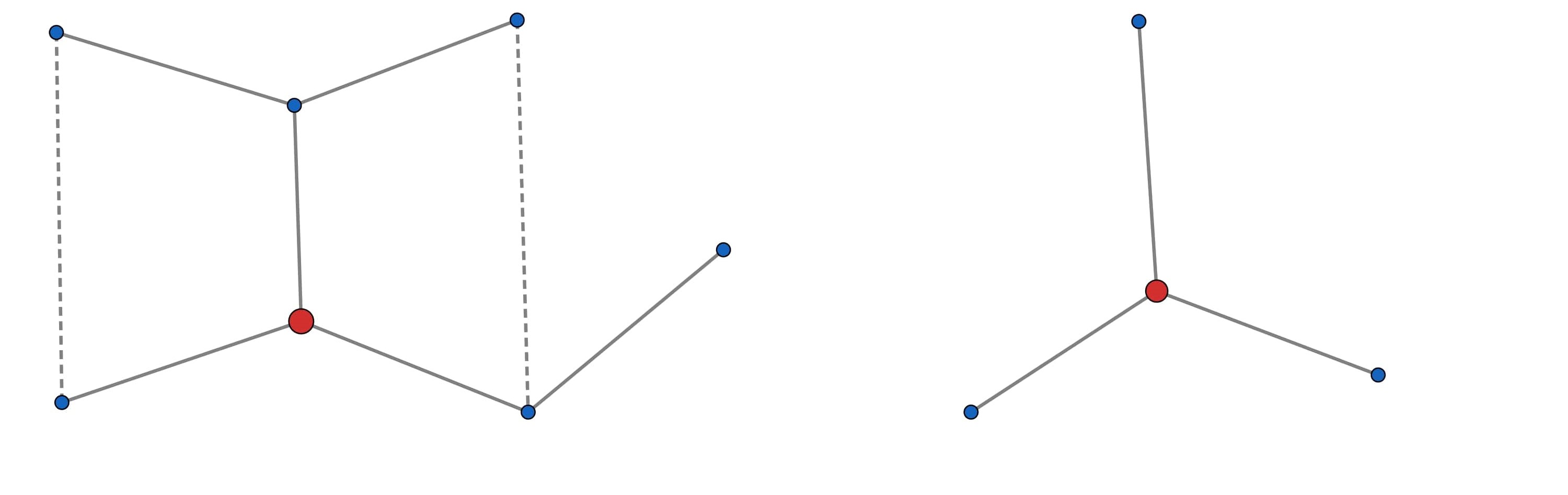
Figure 5. (The construction of the subgraph $T_{W^{\prime}}$ from the graph $G_{W}$) The figure in the left represents the graph $G_{W}$. The center of $T_{W}$ is denoted by a larger red dot. The solid lines represent the edges of a spanning tree $T_{W}$ and the dotted lines the edges of $G_{W}$ not present in $T_{W}$. The figure in the right is obtained from $T_{W}$ by removing the vertices at the distance two from the center of $T_{W}.$

Step II: In this step we establish relation between clique cluster and Type I subgraph.

Lemma 38.

For $p\geq 1,k\geq 3$, let $W=(w_{1},w_{2},\ldots,w_{k})\in\mathcal{W}_{p,k}$ be a sentence such that each letter in $S_{W}$ is repeated at least twice. If $G_{W}$ is connected but not a clique cluster, then $G_{W}$ has a Type I subgraph.

Proof.

The idea of the proof is to provide an explicit construction of the subforest $H_{W}$ with components $T_{1},T_{2},\ldots,T_{r}$ along with the one-one map $\phi$.

Since $G_{W}$ is connected, but not a clique cluster, there exist distinct vertices $i_{1},i_{2},i_{3}$ and letters $a_{1}\in S_{w_{i_{1}}}\cap S_{w_{i_{2}}}$ and $a_{2}\in S_{w_{i_{2}}}\cap S_{w_{i_{3}}}$ with $a_{1}\neq a_{2}$. Add the vertices $i_{1},i_{2},i_{3}$ to $V(T_{1})$ and add the edges $\{\{i_{1},i_{2}\},\{i_{2},i_{3}\}\}$ to $E(T_{1})$ and define $\varphi\left(\{i_{1},i_{2}\}\right)=a_{1}$, $\varphi\left(\{i_{2},i_{3}\}\right)=a_{2}$.

Suppose for all $a\in S_{w_{i_{1}}}\cup S_{w_{i_{2}}}\cup S_{w_{i_{3}}}$, $a$ appears at least twice in $S_{w_{i_{1}}}\cup S_{w_{i_{2}}}\cup S_{w_{i_{3}}}$. Then define $V(T_{1})=\{i_{1},i_{2},i_{3}\}$. If not, then there exists a letter $a_{3}\in S_{w_{i_{1}}}\cup S_{w_{i_{2}}}\cup S_{w_{i_{3}}}$ such that $a_{3}$ appears only once in $S_{w_{i_{1}}}\cup S_{w_{i_{2}}}\cup S_{w_{i_{3}}}$. Since every letter appears at least twice in $S_{W}$, there exist $i_{4}\neq i_{1},i_{2},i_{3}$ such that $a_{3}\in S_{w_{i_{4}}}$. Let $i\in\{i_{1},i_{2},i_{3}\}$ be such that $a_{3}\in S_{w_{i}}$, add the edge $\{i,i_{4}\}$ to the graph and define $\varphi\left(\{i,i_{4}\}\right)=a_{3}$. Since $G_{W}$ is a finite graph, this process should terminate in at most $k_{1}$ steps where $k_{1}\leq k$. Define $T_{1}$ as the graph with vertex set $\{i_{1},i_{2},\ldots,i_{k_{1}}\}$ constructed as above. Note that by construction, $T_{1}$ is a tree such that each letter in $S_{W_{T_{1}}}$ is repeated at least twice and $\varphi:E(T_{1})\rightarrow S_{W}$ is a one-one map. If $\#V(T_{1})=k$, then $H_{W}=T_{1}$ is a Type I subgraph.

Suppose we constructed disjoint subtrees $T_{1},T_{2},\ldots,T_{m}$ with $\#V(T_{i})=k_{i}$, $\kappa=(k_{1}+k_{2}+\cdots+k_{m})<k$ and $k_{i}\geq 2$ for all $1\leq i\leq m$ such that $T_{1},T_{2},\ldots,T_{m}$ obey condition (iii) of Definition 33 and there exists a one-one function $\varphi:\cup_{i=1}^{m}E(T_{i})\rightarrow S_{W}$ obeying condition (iv). Define

$$M_{m}:=\{i \in V(G_{W})\setminus\left(V(T_{1})\cup V(T_{2})\cup\cdots\cup V(T_{m})\right):$$

$$\exists\ a_{\kappa+1}\in S_{w_{i}}\text{ such that }m_{S_{w_{i}}}(a_{\kappa+1})=1\text{ and }a_{\kappa+1}\notin S_{W_{T_{1}}}\cup S_{W_{T_{2}}}\cup\cdots\cup S_{W_{T_{m}}}\}.$$

If $M_{m}$ is empty, then define $H_{W}$ by choosing all the vertices in $G_{W}$ not belonging to $V(T_{1})\cup V(T_{2})\cup\cdots\cup V(T_{m})$ as isolated vertices in $H_{W}$. By construction, $H_{W}$ is a forest. Further, note that as all isolated vertices in $G_{W}$ are grouped together at the last, condition (ii) is also satisfied. Then since $M_{m}$ is empty and by the assumption on $T_{1},T_{2},\ldots,T_{m}$, $H_{W}$ satisfies condition (iii) of Definition 33. Condition (iv) is satisfied as no new edges are added to $H_{W}$ afterwards. As a result, we get that $H_{W}$ is a Type I subgraph.

Suppose $M_{m}$ is not empty. Then define $i_{\kappa+1}=\min\{M_{m}\}$. Since $G_{W}$ is connected, there exist $i_{\kappa+2}\neq i_{\kappa+1}$ such that $a_{\kappa+1}\in S_{w_{i_{\kappa+2}}}$. Construct the edge $\{i_{\kappa+1},i_{\kappa+2}\}$ and define $\varphi\left(\{i_{\kappa+1},i_{\kappa+2}\}\right)=a_{\kappa+1}$.

Suppose for all $a\in S_{w_{i_{\kappa+1}}}\cup S_{w_{i_{\kappa+2}}}$, $a$ appears at least twice in $S_{W_{T_{1}}}\cup S_{W_{T_{2}}}\cup\cdots\cup S_{W_{T_{m}}}\cup S_{w_{i_{\kappa+1}}}\cup S_{w_{i_{\kappa+2}}}$, we define $V(T_{m+1})=\{i_{\kappa+1},i_{\kappa+2}\}$ and $E(T_{m+1})=\{i_{\kappa+1},i_{\kappa+2}\}$. If not, then there exist $a_{\kappa+2}$ that appears only once in $S_{W_{T_{1}}}\cup S_{W_{T_{2}}}\cup\cdots\cup S_{W_{T_{m}}}\cup S_{w_{i_{\kappa+1}}}\cup S_{w_{i_{\kappa+2}}}$, and hence there exist $i_{\kappa+3}$ such that $i_{\kappa+3}\notin V(T_{1})\cup\cdots\cup V(T_{m}),i_{\kappa+3}\neq i_{\kappa+1},i_{\kappa+2}$ and $a_{\kappa+2}\in S_{w_{i_{\kappa+3}}}$. Let $i\in\{i_{\kappa+1},i_{\kappa+2}\}$ such that $a_{i_{\kappa+2}}\in S_{w_{i}}$. Construct the edge $\{i,i_{\kappa+3}\}$ and define $\varphi\left(\{i,i_{\kappa+3}\}\right)=a_{i_{\kappa+2}}$. Continue this construction to obtain a tree $T_{m+1}$ such that for all $a\in S_{W_{T_{m+1}}}$, $a$ appears at least twice in $S_{W_{T_{1}}}\cup S_{W_{T_{2}}}\cup\cdots\cup S_{W_{T_{m+1}}}$. Thus, we have obtained a tree $T_{m+1}$ such that $T_{1},T_{2},\ldots,T_{m+1}$ obey condition (iii) of Definition 33 and there exist a one-one function $\varphi:\cup_{i=1}^{m+1}E(T_{i})\rightarrow S_{W}$ obeying condition (iv).

Continue the construction of trees, and since $G_{W}$ is finite, the construction of trees should stop at some finite step. Define $H_{W}$ as the union of the subtrees along with the isolated vertices. Then by construction, all conditions of Type I subgraph are satisfied by $H_{W}$. Therefore $H_{W}$ is a Type I subgraph and the proof is complete. ∎

Step III: In this final step, using Lemmas 34, 35 and 38 we prove Proposition 24.

Proof of Proposition 24.

Consider a sentence $W=(w_{1},w_{2},\ldots,w_{k})\in\mathcal{W}_{p,k}$ such that $G_{W}$ is connected but not a clique cluster. Then by Lemma 38, $G_{W}$ always has a Type I subgraph. Let $H_{1}$ and $H_{2}$ be Type I subgraphs of $G_{W}$ with respectively one-one maps $\varphi_{1}$ and $\varphi_{2}$. We say $H_{1}\leq H_{2}$, if $H_{1}$ is a subgraph of $H_{2}$ and the restriction of $\varphi_{2}$ to the edge set of $H_{1}$ is $\varphi_{1}$, i.e. $\varphi_{2}|_{E(H_{1})}=\varphi_{1}$. The relation $\leq$ is a partial order on set of all Type I subgraphs of $G_{W}$and we call a maximal element with respect to $``\leq"$ as a maximal Type I subgraph. Since $G_{W}$ is a finite graph, by Lemma 38, maximal Type I subgraphs always exist.

Let $H_{W}$ be a maximal Type I subgraph of $G_{W}$ with associated one-one function $\varphi_{W}$ and let $T_{1},T_{2},\ldots,T_{r}$ be the connected components of $H_{W}$ with $\#V(T_{i})=k_{i}$ for all $i$.

Since $H_{W}$ is a Type I subgraph, $\#V(T_{1})\geq 3$. Furthermore, by condition (iii) of Type I subgraph, each letter in $S_{W_{T_{1}}}$ appears at least twice and therefore, $W_{T_{1}}\in\mathcal{C}_{p,k_{1}}$ where $k_{1}\geq 3$, and $\mathcal{C}_{p,k_{1}}$ is as defined in Definition 32. Thus by Lemma 34, it follows that $\frac{1}{N^{pk_{1}/2}}\#\{\text{choices of }\pi_{T_{1}}\}$ is of the order $o(1)$. Suppose $\pi_{T_{1}},\pi_{T_{2}},\ldots,\pi_{T_{m-1}}$ are chosen. Then, by Remark 37, it follows that the number of choices of $\pi_{T_{m}}$ are given by

$$\frac{1}{N^{pk_{m}/2}}\#\{\text{choices of }\pi_{T_{m}}\}\leq\left\{\begin{array}[]{lll}O(1)&\ \text{ if }k_{m}=2,\\ o(1)&\ \text{ if }k_{m}\geq 3.\end{array}\right.$$

Next we prove a claim for the case when $k_{m}=1$. Claim 1: Let $m$ be such that $k_{m}=1$. Then there exists $a\in S_{W_{T_{m}}}$ such that $a$ appears at least once in $\cup_{i\leq m-1}S_{W_{T_{i}}}$.

Proof of Claim 1.

Suppose for all $a\in S_{W_{T_{m}}}$, $a$ has not appeared in $\cup_{i\leq m-1}S_{W_{T_{i}}}$. Since $G_{W}$ is connected there exist $q>m$ and $x\in S_{W_{T_{m}}}$ such that $x\in S_{W_{T_{q}}}$. Join the vertices in $T_{m}$ and $T_{q}$ by an edge, say $e$, and define $\varphi(e)=x$. Using the construction in Lemma 38, extend this graph to a Type I subgraph $H$ with the one-one function $\varphi$. Then it follows that $H_{W}$ is strictly contained in $H$, contradicting the maximality of $H_{W}$. Thus we have obtained a contradiction. ∎

For $k_{m}=1$, it follows from Claim 1 that there exist $x\in S_{T_{m}}$ such that $x\in S_{T_{i}}$ for some $i<m$. Thus, once all $\pi_{T_{i}}$ such that $\#V(T_{i})\geq 2$ are chosen, the $L$-value of the letter $x$ is fixed. Furthermore, by condition (iii) of Type I subgraph, each new letter in $S_{W_{T_{m}}}$ appears at least twice in $S_{W_{T_{m}}}$. Thus the number of generating vertices of $W_{T_{m}}$ is at most of the order $O(N^{\frac{p-1}{2}+1})=O(N^{\frac{pk_{m}+k_{m}}{2}})$. Hence,

$$\text{number of choices for }(\pi_{1},\pi_{2},\ldots,\pi_{k}) =o(N^{\frac{pk_{1}+k_{1}}{2}})\times O(N^{\frac{pk_{2}+k_{2}}{2}})\times\cdots\times O(N^{\frac{pk_{t}+k_{t}}{2}})$$

$$=o(N^{\frac{pk+k}{2}}),$$

where the last equality follows since $k_{1}+k_{2}+\cdots+k_{t}=k$. This proves the proposition. ∎

5. Applications of Theorem 17

In this section, we show that Theorem 17 can be used to establish that the LES of a large class of random matrices converges to Gaussian distribution. In Section 5.1, we show that if $\Delta_{n}$ obeys Assumption V, then condition (iii) of Theorem 13 holds for most of the classical link functions. In Sections 5.2, 5.3 and 5.4, we show that the two sufficient conditions in Theorem 17 can easily be verified for most of the well-known patterned random matrices. More precisely, in Section 5.2, we discuss LES of classical patterned matrices such as symmetric Toeplitz, Hankel and circulant type matrices; in Section 5.3, we discuss block patterned matrices; and in Section 5.4, we discuss $d$-disco matrix, checkerboard matrix and the swirl matrix. In this section, we always treats the constants $c_{1},c_{2}$ and the sets $\mathcal{Z}_{n},\mathcal{S}_{n}$ as used in Theorem 17, and $\eta_{p}$ as defined in (10).

5.1. Existence of limiting second moment:

In this section, our aim is to check that for a sufficiently large class of link functions $\left\{L_{n}\right\}$, $\lim_{n\rightarrow\infty}\frac{1}{N\frac{p+1}{2}}\#\Pi_{L_{n},\Delta_{n}}(W)$ exist for all $W\in P_{2}(p,p)\cup P_{2,4}(p,p)$. The following is our main theorem.

Theorem 39.

Let $\left\{L_{n}\right\}$ be a sequence of link functions in one of the following forms:

1. $L_{n}(i,j)=i\pm j.$

2. $L_{n}(i,j)=|i-j|$.

3. $L_{n}(i,j)=(i\pm j)\bmod N$ or $|i\pm j|\bmod N$, where $N$ is the dimension of the matrix.

Suppose $\{\Delta_{n}\}$ obeys Assumption V. Then for each $W\in{\mathcal{P}}_{2}(p,p)\cup{\mathcal{P}}_{2,4}(p,p)$,

$$\theta(W)=\lim_{n\rightarrow\infty}\frac{1}{N^{p+1}}\#\Pi_{L_{n},\Delta_{n}}(W)\text{ exist. }$$

Proof of (i).

We shall show that the result is true for $L_{n}(i,j)=i+j$ and the proof for $L_{n}(i,j)=i-j$ follows along similar lines. First we calculate the number of possibilities of $(\pi_{1},\pi_{2})\in\Pi_{L_{n},\Delta_{n}}^{*}(W)$ for $W\in{\mathcal{P}}_{2}(p,p)\cup{\mathcal{P}}_{2,4}(p,p)$. For the purpose of the proof, we denote

$$v_{u,j}=\frac{\pi_{u}(j)}{N}.$$

We prove the proposition for $W\in{\mathcal{P}}_{2,4}(p,p)$ and $W\in{\mathcal{P}}_{2}(p,p)$ separately. First, fix $W=(w_{1},w_{2})\in{\mathcal{P}}_{2,4}(p,p)$. Since $L_{n}(i,j)=i+j$, it follows from (2.1) that if $w_{u_{1}}[j_{1}]=w_{u_{2}}[j_{2}]$, then

$$v_{u_{1},j_{1}-1}+v_{u_{1},j_{1}}=v_{u_{2},j_{2}-1}+v_{u_{2},j_{2}}.$$ (29)

Note that since $\pi_{u}(j)\in[N]$, the value of $v_{u,j}$ must be an integer multiple of $1/N$ less than or equal to one. Also observe that since $W\in{\mathcal{P}}_{2,4}(p,p)$, (29) is a system of equations with $p+1$ equations, where $(p-2)$ equations correspond to blocks of size two and three equations correspond to the block of size four. Additionally, the following equations are also satisfied.

$$v_{1,0}=v_{1,p},\ v_{2,0}=v_{2,p}.$$ (30)

Our aim is to find all values of $v_{u,j}$, multiples of $1/N$, such that (29) and (30) are satisfied. Recall the definition of generating vertices from Definition 26. Define

$$S=\{\text{set of all generating vertices of }W\}$$

and let $v_{S}=\{v_{u,j}:(u,j)\in S\}$. Note that the cardinality of $S$ is $p+1$. We make the following claim:

Claim A. For $u=1,2$ and $0\leq j\leq p$, there exists a linear function $f_{u,j}$ with integer coefficients such that $v_{u,j}=f_{u,j}(v_{S})$.

Proof of Claim A.

Note that the claim holds trivially for all generating vertices $(u,j)$. Let $(u_{1},j_{1})$ be the first non-generating vertex with respect to the dictionary order. Then there exists a generating vertex $(u_{0},j_{0})$ such that $v_{u_{0},j_{0}-1}+v_{u_{0},j_{0}}=v_{u_{1},j_{1}-1}+v_{u_{1},j_{1}}$. Since $(u_{1},j_{1})$ is the first non-generating vertex, $v_{u_{0},j_{0}-1},v_{u_{0},j_{0}}$ and $v_{u_{1},j_{1}-1}$ are elements of $v_{S}$ and therefore $v_{u_{1},j_{1}}=f_{u_{1},j_{1}}(v_{S})$, where $f_{u_{1},j_{1}}(v_{S})$ is a linear function with integer coefficients.

Now suppose $(u_{1},j_{1})$ is a non-generating vertex and for every vertex $(u,j)$ such that $(u,j)<(u_{1},j_{1})$ with respect to the dictionary order, there exist linear functions $f_{u,j}$ with integer coefficients such that $v_{u,j}=f_{u,j}(v_{S})$. Since $W\in{\mathcal{P}}_{2,4}(p,p)$, note that there exists a generating vertex $(u_{0},j_{0})$ such that $v_{u_{0},j_{0}-1}+v_{u_{0},j_{0}}=v_{u_{1},j_{1}-1}+v_{u_{1},j_{1}}$. Since $v_{u_{0},j_{0}-1},v_{u_{0},j_{0}}$ and $v_{u_{1},j_{1}-1}$ are of the form $f_{u,j}(v_{S})$, the claim follows. ∎

Now, we use Claim A to show that the limit $\lim_{n\rightarrow\infty}\frac{1}{N^{p+1}}\#\Pi_{L_{n},\Delta_{n}}^{*}(W)$ exists. Suppose elements of $\{v_{S}\}$ are chosen independently as multiples of $1/N$, and each entry is between 0 and 1. Define $v_{u,j}=f_{u,j}(v_{S})$, where $f_{u,j}$ is as defined in Claim A. Then, note that by the construction of $f_{u,j}$, $\{v_{u,j}:u=1,2,0\leq j\leq p\}$ obeys the system of equations (29). Further since all elements $v_{S}$ are multiples of $1/N$, it follows from Claim A that every $v_{u,j}$ is a multiple of $1/N$. Hence, to check if $\{\pi_{u}(j)=Nv_{u,j}\}$ are elements of $\Pi_{L_{n},\Delta_{n}}^{*}(W)$, it is sufficient to check the following:

1. $0<f_{u,j}(v_{S})\leq 1$ for all $u,j$,

2. the set of equations (30) are satisfied, and

3. $(v_{u,j-1},v_{u,j})\in\frac{\Delta_{n}}{N}$ for $u=1,2$ and $1\leq j\leq p$.

Therefore, we get that $\#\frac{1}{N^{p+1}}\Pi_{L_{n},\Delta_{n}}^{*}(W)$ is the Riemann sum of the integral

$$\int_{[0,1]^{p+1}}\prod_{j=1\atop u=1,2}^{p} {\mathbf{1}}_{[0,1]}\left(f_{u,j}(v_{S})\right)\delta(f_{1,p}(v_{S})=v_{1,0})$$

$$\times\delta(f_{2,p}(v_{S})=v_{2,0})\prod_{j=1\atop u=1,2}^{p}{\mathbf{1}}_{\Delta}\big{(}f_{u,j-1}(v_{S}),f_{u,j}(v_{S})\big{)}dv_{S},$$

with an error term bounded by $2\times\frac{\#\left((\Delta_{n}\setminus\Delta)\cup(\Delta\setminus\Delta_{n})\right)}{N^{2}}$. Since $\Delta_{n}$ obeys Assumption V, it follows that $\#\frac{1}{N^{p+1}}\Pi_{L_{n},\Delta_{n}}(W)$ converges to the above integral as $n\rightarrow\infty$. Now, by Remark 23 (a), the result follows.

Next, we consider $W=(w_{1},w_{2})\in{\mathcal{P}}_{2}(p,p)$. Note that if $w_{u_{1}}[j_{1}]=w_{u_{2}}[j_{2}]$ and $(\pi_{1},\pi_{2})\in\Pi_{L_{n},\Delta_{n}}^{*}(W)$, then (29) and (30) are satisfied. Let $\{(1,r),(2,r^{\prime})\}$ be the last cross-matched block in $W$ (i.e. $r$ is the largest number such that $(1,r)$ is an element of a cross-matched block). For $(w_{1},w_{2})\in{\mathcal{P}}_{2}(p,p)$, we consider the following ordering ‘$\prec$’ on $\{(u,j):u=1,2;j=0,1,2,\ldots,p\}$:

$$(1,0)\prec(1,1)\prec(1,2)\prec\cdots\prec(1,r-1)\prec(1,p)\prec (1,p-1)\prec\cdots\prec(1,r)$$

$$\prec(2,0)\prec(2,1)\prec\cdots\prec(2,p).$$ (31)

Recall from Definition 26 that generating vertices are determined by the ordering on $\{(u,j):u=1,2;j=0,1,2,\ldots,p\}$. Consider the generating vertices of $W$ with respect to the ordering in (5.1) and define

$$S=\{(1,j):j<r\text{ and } (1,j)\text{ is a generating vertex}\}\cup\{(1,j-1):j>r\text{ and }$$

$$(1,j)\text{ is a generating vertex}\}\cup\{(2,j):(2,j)\text{ is a generating vertex}\}.$$ (32)

We define $v_{S}=\{v_{u,j}=\pi_{u}(j)/N:(u,j)\in S\}$, where $S$ is as defined above. Similar to the case $W\in{\mathcal{P}}_{2,4}(p,p)$, the following claim holds.

Claim B. For $u=1,2$ and $0\leq j\leq p$, there exists a linear function $f_{u,j}$, with integer coefficients such that $v_{u,j}=f_{u,j}(v_{S})$, where $S$ is as defined in (5.1).

Proof of Claim B.

Note that the claim holds trivially for vertices $(u,j)\in S$. In the proof of this claim, we use the total ordering ‘$\prec$’ defined in (5.1). Similar to the proof of Claim A, for all non-generating vertices $(1,j)$ such that $j\leq r-1$, it can be shown that $v_{1,j}=f_{1,j}(v_{S})$ where $f_{1,j}$ is a linear function with integer coefficients.

We choose $v_{1,p}=v_{1,0}$ due to (30). Now if $(1,p)$ is a generating vertex, then by the definition of $S$, $v_{1,p-1}\in S$ and the claim holds for $(1,p-1)$. Alternatively, if $(1,p)$ is not a generating vertex with respect to $\prec$, then there exist a generating vertex $(1,j_{0})\prec(1,p)$ such that $v_{1,j_{0}-1}+v_{1,j_{0}}=v_{1,p-1}+v_{1,p}$. Since it is already shown that for all $(1,j)\preceq(1,p)$, $v_{1,j}=f_{1,j}(v_{S})$ where $f_{1,j}$ are linear functions with integer coefficients, it follows that $v_{1,p-1}=f_{1,p-1}(v_{S})$, where $f_{1,p-1}$ is a linear function with integer coefficients. Next, consider $(1,p-1)\prec(1,j)\preceq(1,r)$ and suppose $v_{1,j^{\prime}}=f_{1,j^{\prime}}(v_{S})$ for all $(1,j^{\prime})\prec(1,j)$. For $(1,j)\notin S$, it follows from the definition of $S$ that there exist $(1,j_{0})$ such that $v_{1,j_{0}-1}+v_{1,j_{0}}=v_{1,j}+v_{1,j+1}$. Note that as $v_{1,j_{0}-1},v_{1,j_{0}},v_{1,j+1}\prec v_{1,j}$, the claim follows for $(1,j)$. The case of $(2,1)\preceq(2,j)\preceq(2,p)$ is similar to the case $(1,1)\preceq(1,j)\preceq(1,r)$ and hence the claim is proved for all $(u,j)$. ∎

Note that the cardinality of the set $S$ is $p+1$, as $(1,r)$ is a generating vertex but there is no vertex in $S$ that corresponds to $(1,r)$. Further, by construction, all equations in (29) are satisfied and additionally the equation $v_{1,0}=v_{1,p}$ is also satisfied. Therefore, we get that $\#\frac{1}{N^{p+1}}\Pi_{L_{n},\Delta_{n}}^{*}(W)$ is the Riemann sum of the integral

$$\int_{[0,1]^{p+1}}\prod_{j=1\atop u=1,2}^{p} {\mathbf{1}}_{[0,1]}\left(f_{u,j}(v_{S})\right)\delta(f_{2,p}(v_{S})=v_{2,0})\prod_{j=1\atop u=1,2}^{p}{\mathbf{1}}_{\Delta}\left(f_{u,j-1}(v_{S}),f_{u,j}(v_{S})\right)dv_{S},$$

with an error term bounded by $2\times\frac{\#\left((\Delta_{n}\setminus\Delta)\cup(\Delta\setminus\Delta_{n})\right)}{N^{2}}$. Therefore, $\frac{1}{N^{p+1}}\#\Pi_{L_{n},\Delta_{n}}^{*}(W)$ converges to the above integral as $n\rightarrow\infty$.

Next, note that for $W\in{\mathcal{P}}_{2}(p,p)$,

$$\Pi_{L_{n}}^{*}(W)\setminus\Pi_{L_{n}}(W)=\bigcup_{\tilde{W}}\Pi_{L_{n}}(\tilde{W}),$$

where $\tilde{W}$ is obtained by assigning different letters of $W$ to be the same. Note that $\tilde{W}$ cannot be an element of ${\mathcal{P}}_{2}(p,p)$, and $\#\Pi_{L_{n}}^{*}(\tilde{W})-\#\Pi_{L_{n}}(\tilde{W})$ is of order $O(N^{p+1})$ only if $\tilde{W}\in{\mathcal{P}}_{2,4}(p,p)$. Hence, by Remark 23 (a), it follows that

$$\lim_{n\rightarrow\infty}\frac{1}{N^{p+1}}\Pi_{L_{n}}^{*}(\tilde{W})=\lim_{n\rightarrow\infty}\frac{1}{N^{p+1}}\Pi_{L_{n}}(\tilde{W}),$$

implying that $\frac{1}{N^{p+1}}\Pi_{L_{n}}(\tilde{W})$ converges. ∎

Proof of Theorem 39 (ii) and (iii).

For the case $L_{n}(i,j)=|i-j|$, a sentence $W=(w_{1},w_{2})\in{\mathcal{P}}_{2}(p,p)\cup{\mathcal{P}}_{2,4}(p,p)$, and $(\pi_{1},\pi_{2})\in\Pi_{L_{n},\Delta_{n}}^{*}(W)$, note that if $w_{u_{1}}[j_{1}]=w_{u_{2}}[j_{2}]$, then $L_{n}(\pi_{u_{1}}(j_{1}-1),\pi_{u_{1}}(j_{1}))=L_{n}(\pi_{u_{2}}(j_{2}-1),\pi_{u_{2}}(j_{2}))$, i.e. $\pi_{u_{1}}(j_{1}-1)-\pi_{u_{1}}(j_{1})=\pm\left(\pi_{u_{2}}(j_{2}-1)-\pi_{u_{2}}(j_{2})\right)$.

For each letter in $S_{W}$, fix a choice from $\{+1,-1\}$. Note that in this case, the number of distinct choices are $2^{p}$ for $W\in{\mathcal{P}}_{2}(p,p)$ and $2^{p+1}$ for $W\in{\mathcal{P}}_{2,4}(p,p)$. For each choice, we have a system of equations, as in (29), and the number of solutions of the system of equation can be approximated by a Riemann sum as in part (i). This implies that $\lim_{n\to\infty}\frac{1}{N^{p+1}}\#\Pi^{*}_{L_{n},\Delta_{n}}(W)$ is a finite sum of integrals.

For the case of $L_{n}=(i+j)\mod N$, note that the system of equations can be written as

$$v_{u_{1},j_{1}-1}+v_{u_{1},j_{1}} =v_{u_{2},j_{2}-1}+v_{u_{2},j_{2}}\mod N.$$

$$v_{u_{1},j_{1}-1}+v_{u_{1},j_{1}} -\left(v_{u_{2},j_{2}-1}+v_{u_{2},j_{2}}\right)=kN\text{ for }-2\leq k\leq 2.$$ (33)

For each equation in (5.1), fix a choice of $k$. This leads to a total of $5^{p}$ choice of system of equations for $W\in{\mathcal{P}}_{2}(p,p)$ and $5^{p+1}$ for $W\in{\mathcal{P}}_{2,4}(p,p)$. For each choice of system of equations, $\frac{1}{N^{p+1}}\#\Pi^{*}_{L_{n},\Delta_{n}}(W)$ can be approximated by an appropriate Riemann sum as in part (i). As the number of choices are finite, in this case, $\lim_{n\to\infty}\frac{1}{N^{p+1}}\#\Pi^{*}_{L_{n},\Delta_{n}}(W)$ is a finite sum of integrals. Note that similar arguments also work for $L_{n}(i,j)=|i-j|\mod N$. This completes the proof. ∎

5.2. Classical Patterned Random Matrices:

In this section, we consider some common patterned matrices. To make the calculations simpler, we primarily focus on $N(n)=n$ and $\Delta_{n}=[N]^{2}$, but it can be easily seen that the same conclusions hold for all other choices of $\Delta_{n}$ which satisfying Assumption V. (i) Wigner matrix: Girko was the first to study the linear eigenvalue statistics of Wigner matrices [27]. He obtained CLT type results using Stieltjes transform and martingale techniques and showed that the limiting law is Gaussian. Later, various results on the LES of Wigner matrices were obtained for different modes of convergence and with different types of entries. For an overview, see [31], [55], [38] and [56]. For results on the band and sparse Wigner matrices, see [3], [34] and [54]. For more recent results, see [36], [58]. As observed in [42], the behaviour of Toeplitz, Hankel and circulant matrices differ from Wigner matrices as the number of independent entries is $O(n^{2})$ for Wigner matrices whereas it is $O(n)$ for the other patterned matrices. This makes the scaling $\frac{1}{\sqrt{n}}$ infeasible to study the fluctuations of its LES. It is well known, that the appropriate scaling for Wigner matrix is $1/n^{0}$, and as an implication, for Wigner matrices $\eta_{p}$ defined in (10) converges to the Dirac delta distribution. (ii) Symmetric Toepltiz matrix: To the best of our knowledge, Chatterjee [20] was the first to study the LES of symmetric Toeplitz matrices with random entries. He showed that for test functions $\phi(x)=x^{p_{n}}$, where $p_{n}=o(\log n/\log\log n)$, the LES of symmetric Toeplitz matrices with Gaussian input entries converge to a Gaussian distribution under the total variation norm. Later, Liu et al. [37] studied the LES for symmetric band Toeplitz matrices for independent entries and diagonal entries as zero. They showed that for fixed polynomials, the LES converges in distribution to a Gaussian distribution. The techniques in [37] are only applicable for band Toeplitz matrices with the bandwidth $b_{n}$ such that $b_{n}/n\rightarrow b$ as $n\rightarrow\infty$, and not for anti-band Toeplitz matrices. Here, we provide a generalization of the results in [37] to include a large number of variations, such as the Skyline matrix and anti-band matrices.

We present the case of the usual Toeplitz matrix. Consider the sets

$$\mathcal{Z}_{n} =\{0,1,\ldots,\lfloor\frac{n}{2}\rfloor\}\text{ and}$$

$$\mathcal{S}_{n} =\{(i,j):1\leq i\leq\lfloor\frac{n}{2}\rfloor,1\leq j\leq\lfloor\frac{n}{2}\rfloor+i\}\cup\{(i,j):\lfloor\frac{n}{2}\rfloor+1\leq i\leq n,i+1-\lfloor\frac{n}{2}\rfloor\leq j\leq n\}.$$

Then it is easy to see that (see Figure 6 (b)) that

$$\#\{(i,j):L(i,j)=r_{u}\}\geq n/2\text{ for all }r_{u}\in{\mathcal{Z}}_{n}\text{ and}$$

$$\#(\mathcal{S}_{n}\cap\mathcal{R}_{i})\geq n/2\text{ for all rows }\mathcal{R}_{i}.$$

Further, from Theorem 39 (i), it follows that the second moment of $\eta_{p}$ converges and therefore all conditions of Theorem 13 are satisfied. Now, applying Theorem 17 implies that $\eta_{p}$ converges in distribution to a normal distribution for $p$ even.

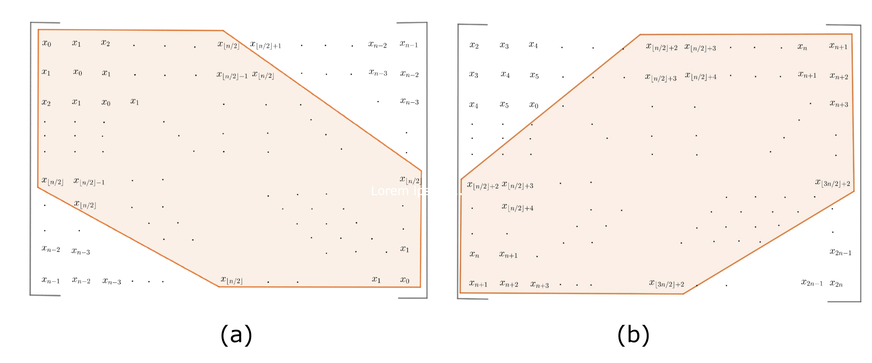
Figure 6. the set $\mathcal{S}_{n}$ is colored in orange for (a) Toeplitz and (b) Hankel

For the odd case, the convergence is trickier. In [37], it was shown that for odd $p$, $\eta_{p}$ converges to the distribution $N(0,\sigma^{2})+x_{0}$, where $N(0,\sigma^{2})$ is an appropriate normal distribution. The calculation of the moments for the distribution shows that for each $k\in\mathbb{N}$, all moments of $x_{i}$ up to order $k$ makes a contribution in $\mathbb{E}(\eta_{p}^{k})$, thereby validating Theorem 18.

(iii) Hankel matrix: The LES for Hankel matrices was first studied in [37], and it was showed that for even $p$, $\eta_{p}$ converges to a normal distribution. To apply Theorem 17, we choose

$$\mathcal{Z}_{n} =\{\lfloor\frac{n}{2}\rfloor+2,\lfloor\frac{n}{2}\rfloor+3,\ldots,\lfloor\frac{3n}{2}\rfloor+2\}\text{ and }$$

$$\mathcal{S}_{n} =\{(i,j):\lfloor\frac{n}{2}\rfloor+2\leq i+j\leq\lfloor\frac{3n}{2}\rfloor+2\}$$

As a result, we get that $c_{1}=c_{2}=1/2$ as in Toeplitz case (see Figure 6 for a pictorial explanation).

For odd $p$, the case is different from the Toeplitz case. It was shown in [1] that for odd $p$, $\eta_{p}$ converges to zero in probability. Later, it was shown in [52] that under the normalization $1/n^{0}$, the moments of $\eta_{p}$ converge to the moments of a non-Gaussian distribution. (iv) Palindromic Toeplitz and Hankel matrices: Palindromic Toeplitz matrices are another important class of patterned random matrices, well-known for having a Gaussian limiting spectral distribution [42]. Palindromic Toeplitz matrix, are obtained from Toeplitz matrices by adding the additional condition $x_{i}=x_{n-1-i}$. To the best of our knowledge, central limit theorem type results for the LES of palindromic Toeplitz matrix are not known. Theorem 17 implies that for even degree monomial test functions, and the choices of $\mathcal{Z}_{n}=\{0,1,2,\ldots,\frac{n}{2}\}$, $c_{1}=c_{2}=1$, the LES of Palindromic Toeplitz matrix converges to a Gaussian distribution.

Palindromic Hankel matrices are obtained from Hankel matrices by imposing the additional condition $x_{i}=x_{n+3-i}$ (so that the first row is a palindrome). Arguments similar to the Palindromic Toeplitz case can be employed for Palindromic Hankel matrix and show that for even $p$, the LES converges to a normal distribution. The result for Palindromic Hankel matrices is also a new addition to the literature. (v) Generalized Toeplitz and Hankel matrices: Several generalizations and alterations of Toeplitz and Hankel matrices, exist in the literature. We talk about the following generalizations introduced in [46].

1. Generalized Toeplitz matrix: For fixed positive integers $\alpha,\beta$, Generalized Toeplitz matrix is the $n\times n$ matrix given by the link function

   $$L_{\alpha,\beta}(i,j):=\begin{cases}\alpha i-\beta j&\mbox{if }i\leq j,\\ -\beta i+\alpha j&\mbox{if }i>j.\end{cases}$$

   For Generalized Toeplitz matrix, we choose

   $${\mathcal{Z}}_{n} =\{\alpha-\beta,\alpha-2\beta,\ldots,\alpha-\lfloor\frac{n}{2}\rfloor\beta\},$$

   $$\mathcal{T}_{n} =\{\left(1+k\beta/d,r+k\alpha/d\right)\in[n]\times[n],k\in\mathbb{N},0\leq r\leq\lfloor\frac{n}{2}\rfloor\},d=\gcd(\alpha,\beta),$$

   $$\mathcal{S}_{n} =\mathcal{T}_{n}\cup\mathcal{T}_{n}^{C},$$

   $$c_{1} =\min\{\frac{dn}{2\alpha},\frac{dn}{2\beta}\}\text{ and }c_{2}=1/2.$$

2. Generalized Hankel matrix: For fixed positive integers $\alpha,\beta$, the link function is given by

   $$L_{\alpha,\beta}(i,j):=\begin{cases}\alpha i+\beta j&\mbox{if }i\leq j,\\ \beta i+\alpha j&\mbox{if }i>j.\end{cases}$$

For Generalized Hankel matrices, we can choose $\mathcal{Z}_{n}$ in a similar fashion as Generalized Toeplitz matrix and this would imply that for Generalized Hankel matrices $\eta_{p}$ converges to Gaussian distribution for all even values of $p$. (vi) Reverse circulant matrix and symmetric circulant matrix: Reverse circulant matrix of dimension $n\times n$ is defined by the link function

$$L(i,j)=(i+j-2)\mod\mbox{n}.$$

For even degree monomial, it is known that $\eta_{p}$ for reverse circulant matrices converges in distribution to a Gaussian distribution with mean zero. This result is established in [43] and the variance formula for the limiting distribution is given in Theorem 4 of [43]. To see the above result as a consequence Theorem 17, note that for the choice of $\mathcal{Z}_{n}=\{0,1,\ldots,n-1\}$, $\mathcal{S}_{n}=[n]^{2}$ , the constants $c_{1}=c_{2}=1$ does the job. Also note that condition (iii) of Theorem 13 follows from part (iii) of Theorem 39.

Hankel matrix is closely related to reverse circulant matrices. A class of Hankel-type matrices was introduced in [7], to study the connection between the LSD of Hankel matrix and reverse circulant matrix. It follows from Theorem 17 that $\eta_{p}$ converges to a normal distribution for even $p$, for matrices in the above class.

For odd degree monomials, it is known that $\eta_{p}$ converges to zero almost surely. Without the scaling $1/\sqrt{n}$, the limiting behavior of the LES of reverse circulant matrix depends on the parity of the order of matrix $n$. This result is discussed in Remark 21 of [43].

Symmetric circulant matrix of dimension $n\times n$ is given by the link function

$$L(i,j)=\frac{n}{2}-|\frac{n}{2}-|i-j||.$$

In [43], it was shown that for these matrices, $\eta_{p}$ converges to normal distribution with mean zero, for both odd and even $p$. To apply Theorem 17, we choose $\mathcal{Z}_{n}=\{0,1,\ldots,n-1\}$, and it follows that the constants are $c_{1}=c_{2}=1$.

The LES for reverse circulant and symmetric circulant matrices were studied in [43] using the explicit values of eigenvalues formula which is well-known in the literature. Thus, the technique of [43] cannot be utilized to obtain the LES of banded versions or other choices of $\Delta_{n}$. Our results give the convergence of LES for banded and anti-banded, reverse circulant and symmetric circulant matrices.

5.3. Block Patterned Matrices:

Here we consider different types of symmetric block patterned matrices, as defined in (1). To the best of our knowledge, all the results in this section are new to the literature. All the block patterned matrices considered in this section will be of the form:

$$A=(B_{L_{1}(i,j)})_{i,j=1}^{d}\text{ with }B_{\ell}=(x_{\ell,L_{2}(i,j)})_{i,j=1}^{m},$$

where $L_{1},L_{2}$ are fixed link functions.

Let $L$ be the link function of the patterned random matrix $A$. Recall the definition of $\Pi_{L}(W)$ from (6) and note that the cardinality of $\Pi_{L}(W)$ depends on $N$, where $[N]$ is the range set of the circuits in $\Pi_{L}(W)$. For the above block patterned random matrix, the appropriate range set of the circuits in $\Pi_{L_{1}}(W)$ is $[d]$, for circuits in $\Pi_{L_{2}}(W)$ is $[m]$, and for circuits in $\Pi_{L}(W)$ is $[md]$. We first prove the following equality:

Proposition 40.

For all $W\in\mathcal{W}_{p,k}$,

$$\#\Pi_{L}^{*}(W)=\#\Pi_{L_{1}}^{*}(W)\times\#\Pi_{L_{2}}^{*}(W).$$

Proof.

We prove the proposition by showing that the map

$$\Pi_{L}^{*}(W) \rightarrow\Pi_{L_{1}}^{*}(W)\times\Pi_{L_{2}}^{*}(W)$$

$$\pi_{u}(i) \rightarrow(\pi_{u}^{(1)}(i),\pi_{u}^{(2)}(i))\text{ for }u=1,2,\ldots,k$$

is a bijection, where

$$\pi_{u}^{(1)}(i)= \frac{\pi_{u}(i)+m-1}{m}\ \text{ and }\ \pi_{u}^{(2)}(i)=\begin{cases}\operatorname{rem}(\pi_{u}(i),m)&\text{ if }m\nmid\pi_{u}(i),\\ m&\text{ if }m|\pi_{u}(i).\end{cases}$$

Note that as $\pi_{u}:\{0,1,\ldots,p\}\rightarrow\{1,2,\ldots md\}$ is a circuit, $\pi_{u}^{(1)}:\{0,1,\ldots,p\}\rightarrow\{1,2,\ldots d\}$ and $\pi_{u}^{(2)}:\{0,1,\ldots,p\}\rightarrow\{1,2,\ldots m\}$ are circuits.

To prove that the map is well-defined, we use the following reasoning: note that for $W\in\mathcal{W}_{p,k}$ and $(\pi_{1},\pi_{2},\ldots,\pi_{k})\in\Pi_{L}(W)$,

$$w_{u_{1}}[i_{1}]=w_{u_{2}}[i_{2}]\implies L(\pi_{u_{1}}(i_{1}-1),\pi_{u_{1}}(i_{1}))=L(\pi_{u_{2}}(i_{2}-1),\pi_{u_{2}}(i_{2}))$$

$$\Longleftrightarrow L_{1}(\pi_{u_{1}}^{(1)}(i_{1}-1),\pi_{u_{1}}^{(1)}(i_{1}))=L_{1}(\pi_{u_{2}}^{(1)}(i_{2}-1),\pi_{u_{2}}^{(1)}(i_{2}))\text{ and }$$

$$L_{2}(\pi_{u_{1}}^{(2)}(i_{1}-1),\pi_{u_{1}}^{(2)}(i_{1}))=L_{2}(\pi_{u_{2}}^{(2)}(i_{2}-1),\pi_{u_{2}}^{(2)}(i_{2})).$$ (34)

This implies that $(\pi_{1}^{(1)},\pi_{2}^{(1)},\ldots,\pi_{k}^{(1)})\in\Pi_{L_{1}}^{*}(W)$ and $(\pi_{1}^{(2)},\pi_{2}^{(2)},\ldots,\pi_{k}^{(2)})\in\Pi_{L_{2}}^{*}(W)$. Note that the values of $\pi_{u}^{(1)}(i)$ and $\pi_{u}^{(2)}(i)$ determine the value of $\pi_{u}(i)$ uniquely and therefore the map is one-one; and the onto property follows from swapping the two sides of the if and only if condition in (5.3). ∎

Now we look at special types of block patterned random matrices and obtain their LES results. (i) Block Wigner matrix: Let $M:\mathbb{N}\to\mathbb{N}$ be an increasing function. Consider the block Wigner matrix given by

$$W_{n}=\left[\begin{array}[]{cccccc}A_{11}(n)&\cdots&A_{1d}(n)\\ \vdots&\ddots&\vdots\\ A_{1d}(n)&\cdots&A_{dd}(n)\end{array}\right],$$

where $d\in\mathbb{N}$ is fixed and for each $n\in\mathbb{N}$, $\{A_{i,j}(n)\}$ are $M(n)\times M(n)$ independent patterned random matrices with link function $L_{2}$. Then the value of $\#\Pi_{L_{1}}(W)$ is a constant, depending only on $p,n$ and $L_{1}$.

Suppose $\{A_{ij}(n)\}$ is one of the classical patterned random matrices discussed in Section 5.2. Then it follows from the discussions in Section 5.2 that

$$\frac{1}{(M(n))^{p+1}}\#\Pi_{L_{2}}(W)$$

converges to a constant strictly greater than zero. As a result, we get using Proposition 40 that

$$\frac{1}{N^{p+1}}\#\Pi_{L}(W)=\frac{1}{d^{p+1}}\#\Pi_{L_{1}}(W)\times\frac{1}{(M(n))^{p+1}}\#\Pi_{L_{2}}(W).$$

Here $L_{1}$ is the link function of Wigner matrix. Since, the number of blocks is fixed, $\frac{1}{d^{p+1}}\#\Pi_{L_{1}}(W)$ is a constant independent of $n$ and strictly greater than zero. Hence, the second moment of $\eta_{p}$ for block Wigner matrix converges to a constant greater than zero. This implies that for block Wigner matrices with fixed number of blocks, $\eta_{p}$ converges in distribution to a Gaussian distribution for even $p$.

(ii) Block Toeplitz and Block Hankel matrices: Let $\{A_{i}:i\in\mathbb{Z}_{+}\}$ be a sequence of independent random matrices of size $M\times M$ of the form (3). The block Toeplitz matrix of size $Md(n)\times Md(n)$ with blocks $(A_{i})$, is defined as $T_{i,j}=A_{i+j}$. For block Toeplitz matrix with independent Wigner blocks of fixed size, the LSD was derived in [9], and LSD for block size growing to infinity was derived in [35],[25]. The fluctuations of the LES of block Toeplitz and block Hankel matrices have not been studied yet.

Consider a block Toeplitz matrix with independent Wigner blocks of fixed size $M$. It is easy to see that the argument for Toeplitz matrices works for this case and conditions (i) and (ii) of Theorem 17 hold for block Toeplitz matrices as well. From Proposition 40, we have

$$\frac{1}{N^{p+1}}\#\Pi_{L}(W)=\frac{1}{d^{p+1}}\#\Pi_{L_{1}}(W)\times\frac{1}{M^{p+1}}\#\Pi_{L_{2}}(W).$$

Note that here $M$, the size of the blocks are fixed, and therefore $\frac{1}{M^{p+1}}\#\Pi_{L_{2}}(W)$ is a constant strictly greater than zero. Further, since $L_{1}$ is the link function of Toeplitz matrix, $\frac{1}{d(n)^{p+1}}\#\Pi_{L_{1}}(W)$ converges. Hence, for the case of block Toeplitz matrices with independent Wigner blocks of fixed size, it follows that for even degree monomials, the LES converges to Gaussian distribution.

For the case where the blocks are other classical patterned random matrices given in Section 5.2, a broader result is possible. Consider the block Toeplitz matrix of size $M(n)\times M(n)$ with symmetric circulant blocks of size $d(n)\times d(n)$. In this case, note that both $\frac{1}{M(n)^{p+1}}\#\Pi_{L_{2}}(W)$ and $\frac{1}{d(n)^{p+1}}\#\Pi_{L_{1}}(W)$ converge to constants greater than zero as $d,n\rightarrow\infty$. Thus, it follows that for all choice of increasing functions $d,M:\mathbb{N}\rightarrow\mathbb{N}$, the LES converges to a Gaussian distribution for even degree monomials. The same conclusion also hold for other patterned blocks.

For block Hankel matrices too, the same conclusions hold, and the calculations are similar to the block Toeplitz case.

(iii) Block versions of circulant-type Matrix: The LSD of block symmetric circulant matrix with Wigner blocks was derived in [48],[32] and more general ensemble in [57]. The problem of fluctuations of LES for block symmetric circulant matrices has not been derived yet. Clearly, Theorem 17 can be applied here for different choices of the blocks, such as Wigner blocks or Hankel blocks. One can use a similar technique as used for Block Toeplitz matrices to conclude the LES results for circulant-type block matrices.

5.4. Extension to other models:

In this section, we discuss some other models of random matrices (apart from the patterned matrices) for which Theorem 17 can be applied. The LES for the random matrices discussed in this section is new to the literature. (i) $d$-disco matrix: This matrix was first introduced and studied in [11] to study the transition of the limiting spectral distribution from Gaussian (for Palindromic Toeplitz) to semi-circle law (for Wigner). Consider a symmetric random matrix $A$ of dimension $M\times M$ and a sequence of patterned random matrices $\{B_{n}:n\in\mathbb{N}\}$ such that $B_{n}$ is of the order $2^{n}M\times 2^{n}M$, the $d$-disco of $A,\{B_{n}\}$ is defined inductively as

$$\mathcal{D}_{n}=\left(\begin{array}[]{cc}\mathcal{D}_{n-1}&B_{n}\\ B_{n}&\mathcal{D}_{n-1}\end{array}\right)\mbox{ with }\mathcal{D}_{0}=A.$$

Suppose there exist fixed constants $c_{1},c_{2}>0$, independent of $n$, such that $B_{n}$ obeys conditions (i) and (ii) of Theorem 17 for all $k$. Then it follows that $\mathcal{D}_{n}$ also obeys conditions (i) and (ii). In particular it can easily be seen that the new constants are $c_{1}^{\prime}=c_{1}/2$ and $c_{2}^{\prime}=c_{2}/2$. Hence, assuming the convergence of the second moment of the LES, we get that the LES converges to a Gaussian distribution for even degree monomial test functions.

(ii) Checkerboard matrix: Let $\{x_{i}:i\in\mathbb{Z}^{d}\}$ be an input sequence. For $k\in\mathbb{N},w\in\mathbb{R}$, and a link function $L_{n}:\mathbb{Z}^{2}\rightarrow\mathbb{Z}^{d}$, the $N\times N$ $(k,w)$-checkerboard ensemble is the matrix $M=\left(m_{ij}\right)$ given by

$$m_{ij}=\begin{cases}x_{L_{n}(i,j)}&\text{ if }i\not\equiv j\bmod k,\\ w&\text{ if }i\equiv j\bmod k.\end{cases}$$

In [19], Burkhardt et al. introduced Checkerboard matrix and studied its LSD.

For $w=0$, the checkerboard matrix is a special case of the matrix defined in (3). Thus by Theorem 17, it follows that when $L_{n}$ is one of the classical link functions, the LES of $(k,0)$-checkerboard matrix converges to a Gaussian distribution for even degree monomial test functions. (iii) Swirl Matrix: The swirl of two $N\times N$ matrices $A$ and $X$ is defined as

$$\operatorname{swirl}(A,X)=\left(\begin{array}[]{cc}AX&A\\ XAX&XA\end{array}\right).$$

Swirl matrices were introduced in [23] to study the LSD of circulant Hankel matrices. Note that when $X$ is a permutation matrix and $A$ is a generalized patterned random matrix of the form (3), $\operatorname{swirl}(A,X)$ is also of the form (3). Then $\operatorname{swirl}(A,X)$ is a symmetric matrix. Suppose $A$ is a patterned random matrix obeying the conditions (i) and (ii) of Theorem 17. Then it follows that $\operatorname{swirl}(A,X)$ also obeys all the conditions of Theorem 17, and as a result its LES converge to a normal distribution for all even degree monomials.

6. LES for Brownian motion entries

In this section, we prove Theorem 20. We first briefly explain the central ideas and preliminaries required for the proof of Theorem 20.

6.1. Preliminaries

Consider the measurable space $(C_{\infty},\mathcal{C_{\infty}})$, where $C_{\infty}:=C[0,\infty)$ is the space of all real-valued continuous functions on $[0,\infty)$ with the following metric.

$$d(f,g)=\sum_{k=1}^{\infty}2^{-k}\frac{d_{[0,k]}(f,g)}{1+d_{[0,k]}(f,g)},$$ (35)

with $d_{[0,k]}$ denoting the supremum metric on $C[0,k]$, and $\mathcal{C_{\infty}}$ is the Borel $\sigma$-field generated by open sets of $C_{\infty}$. For a probability space $\left(\Omega,\mathcal{F},\mathbb{P}\right)$, we define a continuous process on $\Omega$ as a $C_{\infty}$-valued random variable. For more details about $(C_{\infty},\mathcal{C_{\infty}})$, see [30], [50] or [33]. The following definition provides the notion of distributional convergence of processes.

Definition 41.

Suppose $\{\bm{X_{n}}\}_{n\geq 1}$ = $\{X_{n}(t);t\geq 0\}_{n\geq 1}$ and $\bm{X}=\{X(t);t\geq 0\}$ are real-valued continuous processes on $\Omega$. We say $\bm{X_{n}}$ converges to $\bm{X}$ weakly or in distribution, if

$$\int_{C_{\infty}}fd\mbox{P}_{n}\rightarrow\int_{C_{\infty}}fd\mbox{P}\ \mbox{ as }n\to\infty,$$

for every bounded, continuous real-valued function $f$ on $C_{\infty}$, where $\mbox{P}_{n}$ and P are the probability measures on $(C_{\infty},\mathcal{C_{\infty}})$ induced by $\bm{X_{n}}$ and $\bm{X}$, respectively. We shall denote this convergence by $\bm{X_{n}}\stackrel{{\scriptstyle\mathcal{D}}}{{\rightarrow}}\bm{X}$.

Suppose $\{\bm{X_{n}}\}_{n\geq 1}$ = $\{X_{n}(t);t\geq 0\}_{n\geq 1}$ is a sequence of continuous processes on $\Omega$. The following result follows from [Theorem I.4.2, [30]].

Result 42.

Suppose the sequence of continuous processes $\{\bm{X_{n}}\}$ on $\Omega$ obeys the following two conditions

1. Finite dimensional convergence: For all $r\in\mathbb{N}$ and $0\leq t_{1}<t_{2}<\cdots<t_{r}$, as $n\rightarrow\infty$, $(X_{n}(t_{1}),X_{n}(t_{2}),\ldots,X_{n}(t_{r}))$ converges in distribution.

2. Tightness: The sequence $\{\bm{X_{n}}\}_{n\geq 1}$ is tight.

Then there exist a probability space $(\widehat{\Omega},\widehat{\mathcal{F}},\widehat{\mathbb{P}})$ and continuous processes $\bm{\widehat{X}_{n}},\widehat{\bm{X}}$ on $\widehat{\Omega}$ such that $\bm{\widehat{X}_{n}}\stackrel{{\scriptstyle D}}{{\sim}}\bm{X_{n}}$ for each $n$ and $\bm{\widehat{X}_{n}}$ converges to $\widehat{\bm{X}}$ almost surely, where $g\mathbin{\overset{D}{\kern 0.0pt\sim}}h$ denotes that $g$ and $h$ have the same distribution.

Since $\widehat{\bm{X}}$ is a continuous process, it defines a probability measure $\mu_{\widehat{X}}$ on $(C_{\infty},\mathcal{C_{\infty}})$. Here, we say that $\bm{X_{n}}$ converges in distribution to $\mu_{\widehat{X}}$. The following result provides the existence of a continuous process on $\Omega$ with distribution $\mu_{\widehat{X}}$.

Result 43 (Lemma 2, [10]).

Suppose $\mathcal{D}$ is a Polish space and $X_{n}:\Omega\rightarrow\mathcal{D}$ converges in distribution to a probability measure $\mu$ on $\mathcal{D}$. Then on the probability space $(\Omega,\mathcal{F},\mathbb{P})$, there is a measurable map $X:\Omega\rightarrow\mathcal{D}$ with distribution $\mu$.

It is known that $C_{\infty}$ is a Polish space under the metric (35). Therefore, it follows from Result 43 that for any sequence $\{\bm{X_{n}}\}$ on $\Omega$ obeying the conditions (i) and (ii) of Result 42 there exists a continuous process $\bm{X}$ on $\Omega$ such that $\bm{X_{n}}\stackrel{{\scriptstyle D}}{{\rightarrow}}\bm{X}$.

Recall the definition of the process $\{\kappa_{p}(t)\>t\in[0,\infty)\}$ from (12) and note that $\kappa_{p}(t)$ depends on $n$ as well. For proving Theorem 20, our objective is to establish the convergence of the process $(\kappa_{p}(t);t\geq 0)$ from the convergence of the random variables $\{\kappa_{p}\}$. In Lemma 47, we show that $\mathbb{E}[q(\kappa_{p}(t_{1}),\ldots,\kappa_{p}(t_{r}))]$ converges for all monomials $q\in\mathbb{R}[x_{1},\ldots,x_{r}]$. Using Lemma 47 and multi-dimensional moment method (Result 46), we establish the finite dimensional convergence (see Lemma 49). Later, the tightness of the sequence is established in Section 6.3.

Take $\bm{X_{n}}(t)$ = $\kappa_{p}(t)$, where $\kappa_{p}(t)$ is as defined in (12). Note that from Result 42 and [30, Theorem I.4.3], Theorem 20 follows from the following two propositions.

Proposition 44.

Let $p$ be a positive integer. Then for any $r\in\mathbb{N}$ and $0\leq t_{1}<t_{2}<\cdots<t_{r}$, as $n\rightarrow\infty$, $(\kappa_{p}(t_{1}),\kappa_{p}(t_{2}),\ldots,\kappa_{p}(t_{r}))$ converges in distribution.

Proposition 45.

For each positive integer $p$, there exist positive constants $C$ and $\gamma$ such that

$$\mathbb{E}{|\kappa_{p}(0)|^{\gamma}}\leq C\ \ \ \forall\ n\in\mathbb{N}.$$

Furthermore, there exist positive constants $\alpha,\beta$ and $M_{T}$, $T=1,2,\ldots$ such that

$$\mathbb{E}{|\kappa_{p}(t)-\kappa_{p}(s)|^{\alpha}}\leq M_{T}|t-s|^{1+\beta}\ \ \ \forall\ n\in\mathbb{N}\ \mbox{and }t,s\in[0,\ T],(T=1,2,\ldots).$$ (36)

Proposition 44 yields the finite dimensional convergence of the process $\{\kappa_{p}(t);t\geq 0\}$ and Proposition 45 provides the tightness of the process $\{\kappa_{p}(t);t\geq 0\}$.

6.2. Finite Dimensional Convergence:

Our approach in proving Proposition 44 is through the multi-dimensional moment method. The following result provides the method.

Result 46 (Theorem 1, [29]).

Let $\mu_{n}$ and $\mu$ be probability measures on $\mathbb{R}^{r}$. Suppose that $\mu$ is uniquely determined by its moments and

$$\lim_{n\to\infty}\int_{\mathbb{R}^{r}}x_{1}^{k_{1}}x_{2}^{k_{2}}\cdots x_{r}^{k_{r}}\mu_{n}(dx_{1},\ldots,dx_{r})=\int_{\mathbb{R}^{r}}x_{1}^{k_{1}}x_{2}^{k_{2}}\cdots x_{r}^{k_{r}}\mu(dx_{1},\ldots,dx_{r}),$$ (37)

for all $k_{1},k_{2},\ldots,k_{r}\in\{0,1,2,\ldots\}$. Then $\mu_{n}\stackrel{{\scriptstyle d}}{{\rightarrow}}\mu$.

For a fixed $r\in\mathbb{N}$ and $0\leq t_{1}<t_{2}<\cdots<t_{r}$, consider the $r$-dimensional random vector $(\kappa_{p}(t_{1}),\kappa_{p}(t_{2}),\ldots,\kappa_{p}(t_{r}))$. For a monomial $q$ on $r$ variables, we define the joint moment of an $r$-dimensional vector $(Y_{1},Y_{2},\ldots,Y_{r})$ as $\mathbb{E}[q(Y_{1},Y_{2},\ldots,Y_{r})]$. In the following proposition we show that $\mathbb{E}\left[q\left(\kappa_{p}(t_{1}),\ldots,\kappa_{p}(t_{r})\right)\right]$ is convergent for every choice of monomial $q$.

Lemma 47.

Let $\{L_{n}:[N]^{2}\rightarrow\mathbb{Z}^{d}\}$ be a sequence of link functions obeying Assumption IV, $\Delta_{n}\subseteq[N]^{2}$ and let $A_{n}(t)=(a_{L_{n}(i,j)}(t){\mathbf{1}}_{\Delta_{n}}(i,j))_{i,j=1}^{N}$ be the symmetric matrix-valued stochastic process corresponding to $L_{n}$ with input sequence $\{a_{i}(t)\}$, where $\{a_{i}(t)\}$ are independent Brownian motions. Suppose all moments of $\kappa_{p}$ converge where $\kappa_{p}$ as in (13). Then for every choice of $0\leq t_{1}<t_{2}<\cdots<t_{r}$ and $q\in\mathbb{R}[x_{1},x_{2},\ldots,x_{r}]$, $\mathbb{E}\left[q\left(\kappa_{p}(t_{1}),\ldots,\kappa_{p}(t_{r})\right)\right]$ converges.

Proof.

First recall the definition of $\kappa_{p}(t)$ from (12). To prove Lemma 47, it is sufficient to show that $\mathbb{E}\left[q\left(\kappa_{p}(t_{1}),\ldots,\kappa_{p}(t_{r})\right)\right]$ converges for all monomials $q$ on $r$ variables. For $k_{1},k_{2},\ldots,k_{r}\in\mathbb{N}$, consider $q[x_{1},x_{2},\ldots,x_{r}]=x_{1}^{k_{1}}x_{2}^{k_{2}}\cdots x_{r}^{k_{r}}$. Similar to (3.1), we have

$$\mathbb{E}[\kappa_{p}^{k_{1}}\left(t_{1}\right)\kappa_{p}^{k_{2}}\left(t_{2}\right)\cdots\kappa_{p}^{k_{r}}\left(t_{r}\right)]=\frac{1}{N^{\frac{pk+k}{2}}}\sum_{W\in\mathcal{W}_{p,k}}\sum_{\Pi_{L_{n},\Delta_{n}}(W)}\mathbb{E}\left(\prod_{i=1}^{k}\big{(}a_{\pi_{i}}(t_{i})-\mathbb{E}a_{\pi_{i}}(t_{i})\big{)}\right),$$ (38)

where the summation is over $(\pi_{1},\pi_{2},\ldots,\pi_{k})\in\Pi_{L_{n},\Delta_{n}}(W)$, and for any $m\in\{1,2,\ldots,r\}$, $t_{i}=t_{m}$ when $k_{1}+k_{2}+\cdots+k_{m-1}<t_{i}\leq k_{1}+k_{2}+\cdots+k_{m}$. Note that, since $a_{i}(t)$ are i.i.d. Brownian motion entries, $\mathbb{E}\left(\prod_{i=1}^{k}\left(a_{\pi_{i}}(t_{i})-\mathbb{E}a_{\pi_{i}}(t_{i})\right)\right)$ in (38) depends only on the sentence $W=(w_{1},w_{2},\ldots,w_{k})$ and is fixed for every choice of $(\pi_{1},\pi_{2},\ldots,\pi_{k})\in\Pi_{L_{n},\Delta_{n}}(W)$ and we denote it by $\mathbb{E}\left(\prod_{i=1}^{k}\left(a_{w_{i}}(t_{i})-\mathbb{E}a_{w_{i}}(t_{i})\right)\right)$. Furthermore, we denote

$$v(W)=\frac{\#\Pi_{L_{n},\Delta_{n}}(W)}{N^{\frac{pk+k}{2}}}\mathbb{E}\left(\prod_{i=1}^{k}(a_{w_{i}}(t_{i})-\mathbb{E}a_{w_{i}}(t_{i}))\right).$$ (39)

Consider a letter, say $a\in S_{W}$ such that $a$ appears $q_{a}$ times in $S_{W}$ and suppose that the appearances of the letter $a$ are given by $a(t_{1,a}),a(t_{2,a}),\ldots,a(t_{q_{a},a})$.

Note from the property of Brownian motion that for any $a(t_{i,a})$, $a(t_{1i,a})\mathbin{\overset{D}{\kern 0.0pt\sim}}\sqrt{t_{i,a}}x$, where $x$ has the distribution $N(0,1)$. Since $t_{i,a}\leq t_{r}$ for all $1\leq i\leq q_{a}$, it follows from the computation of joint moments of Brownian motions (Lemma 4.5,[39]) that $\mathbb{E}[a(t_{1,a})a(t_{2,a})\cdots a(t_{q_{a},a})]\leq t_{r}^{q_{a}/2}\mathbb{E}[x^{q_{a}/2}]$. Thus, we get that for $W\in\mathcal{W}_{p,k}$,

$$|v(W)| \leq\frac{\#\Pi_{L_{n},\Delta_{n}}(W)}{N^{\frac{pk+k}{2}}}\big{|}\mathbb{E}\Big{[}\prod_{s=1}^{r}(t_{s})^{\frac{pk_{s}}{2}}\prod_{i=1}^{k_{s}}\big{[}\frac{a_{w_{i}}(t_{s})}{\sqrt{t_{s}}}-\mathbb{E}[\frac{a_{w_{i}}(t_{s})}{\sqrt{t_{s}}}]\big{]}\Big{]}\big{|}$$

$$\leq\frac{\#\Pi_{L_{n},\Delta_{n}}(W)t_{r}^{\frac{pk}{2}}}{N^{\frac{pk+k}{2}}}\Big{|}\mathbb{E}\left[\prod_{i=1}^{k}(x_{w_{i}}-\mathbb{E}x_{w_{i}})\right]\Big{|},$$ (40)

where $\{x_{i}\}$ are independent standard normal random variables. As $\{L_{n}\}$ satisfies Assumption IV and $\{x_{i}\}$ satisfies Assumption I, it follows from Proposition 24 that (6.2) is of the order $o(1)$ if $W\notin SP(p,k)$.

Consider $W\in SP(p,k)$. We have that for all clusters $C$ of $W$, $W_{C}$ is an element of ${\mathcal{P}}_{2}(p,p)$ or ${\mathcal{P}}_{2,4}(p,p)$ or a clique sentence. Direct computation using Lemma 4.5 of [39] yields that

$$\mathbb{E}\left[\prod_{i\in V(C)}(a_{w_{i}}(t_{i})-\mathbb{E}a_{w_{i}}(t_{i}))\right]=\begin{cases}\prod_{u=1}^{s}t_{i_{u}}^{s-u}\prod_{u=1}^{s}(t_{i_{u}})^{\frac{p-1}{2}}&\text{ if }W_{C}=(w_{i_{1}},\ldots,w_{i_{s}})\text{ is}\\ &\ \ \text{ a clique sentence},\\ t_{i_{1}}^{\frac{p+c_{0}}{2}}t_{i_{2}}^{\frac{p-c_{0}}{2}}&\text{ if }W_{C}=(w_{i_{1}},w_{i_{2}})\in{\mathcal{P}}_{2}(p,p),\\ \\ t_{i_{1}}^{\frac{p}{2}-1}t_{i_{2}}^{\frac{p}{2}-1}(2t_{i_{1}}+t_{i_{2}}-t_{i_{1}}t_{i_{2}})&\text{ if }W_{C}=(w_{i_{1}},w_{i_{2}})\in{\mathcal{P}}_{2,4}(p,p),\end{cases}$$

where $c_{0}$ is the number of cross-matched entries between $w_{i_{1}}$ and $w_{i_{2}}$ for $(w_{i_{1}},w_{i_{2}})\in{\mathcal{P}}_{2}(p,p)$. In the above expression we have chosen $t_{i_{1}}<t_{i_{2}}<\cdots$, and this is valid as the value of $v(W)$ does not change under permutation of words. Now, by using condition (iii) of Theorem 18, we get that $v(W)$ converges. This completes the proof. ∎

Now using Haviland’s theorem we show that the limits of sequence of joint moments determine a distribution. The uniqueness of this distribution is established by using its connection to the one-dimensional determinate problem. We state the following result due to Haviland.

Result 48 (Theorem 3.1.2, [40], Haviland’s Theorem).

For a linear function $L:\mathbb{R}[x_{1},x_{2},\ldots,x_{r}]\rightarrow\mathbb{R}$, and a closed set $K$ in $\mathbb{R}^{r}$, the following are equivalent:

1. there exists a probability measure $\mu$ on $K$ such that

   $$L(f)=\int f\cdot\mathrm{d}\mu\quad\forall\ f\in\mathbb{R}[x_{1},x_{2},\ldots,x_{r}].$$ (41)

2. $L(f)\geq 0$, for all $f\in\mathbb{R}[x_{1},x_{2},\ldots,x_{r}]$ such that $f\geq 0$ in $K$ and $L(\mathbf{1})=1,$ where $\mathbf{1}$ is the constant function with range $\{1\}$.

The following theorem provides the existence and uniqueness of a distribution whose moments are the limiting sequence of joint moments of the process $\{\kappa_{p}(t):t\geq 0\}$.

Lemma 49.

For fixed $0\leq t_{1}<t_{2}<\cdots<t_{r}$ and $q\in\mathbb{R}[x_{1},x_{2},\ldots,x_{r}]$, let

$$\Pi_{q}:=\lim_{n\rightarrow\infty}\mathbb{E}\left[q\left(\kappa_{p}(t_{1}),\ldots,\kappa_{p}(t_{r})\right)\right]$$ (42)

exist. Further, suppose that the moments of $\kappa_{p}$ is $M$-determinate. Then there exists a unique distribution $\Gamma_{t_{1},t_{2},\ldots,t_{r}}$ in $\mathbb{R}^{r}$ with the joint moments as

$$\mathbb{E}(q\left(\Gamma_{t_{1},t_{2},\ldots,t_{r}})\right)=\Pi_{q}.$$ (43)

Proof.

We prove the existence part by using Result 48. Recall that $\kappa_{p}(t_{r})$ depends on $n$. For a fixed $n$, let $F_{n}$ denote the distribution of $\left(\kappa_{p}(t_{1}),\kappa_{p}(t_{2}),\ldots,\kappa_{p}(t_{r})\right)$ in $\mathbb{R}^{r}$.

Consider the sequence of linear maps $L_{n}:\mathbb{R}[x_{!},x_{2},\ldots,x_{r}]\rightarrow\mathbb{R}$ defined by

$$L_{n}(q):=\int q(x_{1},x_{2},\ldots,x_{r})\mathrm{d}F_{n}.$$

By Haviland’s theorem, we obtain that $L_{n}(q)\geq 0$ for all $q\in\mathbb{R}[x_{1},x_{2},\ldots,x_{r}]$ such that $q\geq 0$ on $\mathbb{R}^{r}$.

Now for $q\in\mathbb{R}[x_{1},x_{2},\ldots,x_{r}]$, we define

$$L(q):=\Pi(q)=\lim_{n\rightarrow\infty}L_{n}(q).$$ (44)

Clearly, $L$ is a linear map. Further note from (44) that $L(q)\geq 0$ for all $q\in\mathbb{R}[x_{1},x_{2},\ldots,x_{r}]$ such that $q\geq 0$ on $\mathbb{R}^{r}$. Therefore from Haviland’s theorem, we get the existence of a measure. Further, since $F_{n}$ are probability distributions, we get that $L_{n}(\mathbf{1})=1$ and as a result we get that $L(\mathbf{1})=1$, and that the measure is a probability measure.

Note from Theorem 3 of [49] that to prove the uniqueness of $\Gamma_{t_{1},t_{2},\ldots,t_{r}}$, it is sufficient to show that for each $i=1,2,\ldots,r$, the moment sequence $\{m_{k}^{(t_{i})}=\mathbb{E}[\kappa_{p}(t_{i})]^{k}\}$ uniquely determines a measure on $\mathbb{R}$. Now recall that

$$\kappa_{p}(t_{i})=\frac{1}{N^{\frac{p+1}{2}}}\left[{\mbox{Tr}}\left(\frac{A_{n}(t_{i})}{\sqrt{N}}\right)^{p}-\mathbb{E}{\mbox{Tr}}\left(\frac{A_{n}(t_{i})}{\sqrt{N}}\right)^{p}\right],$$

where $A_{n}(t_{i})$ is a random matrix with independent standard Brownian motion entries $\{a_{j}(t_{i})\}$. For a fixed $t_{i}$, $y_{j}:=a_{j}(t_{i})/\sqrt{t_{i}}$ satisfies Assumption II. Observe that for $\kappa_{p}$ defined in (13) has input sequence $\{y_{j}\}$, and the limiting moment sequence of $\kappa_{p}$ is M-determinate. Hence, $\{\frac{m_{k}^{(t_{i})}}{t_{i}^{p/2}}\}$ defines a unique measure on $\mathbb{R}$, which in turn implies that $\{m_{k}^{(t_{i})}\}_{k\in\mathbb{N}}$ determines a unique measure on $\mathbb{R}$. ∎

It follows from Lemma 49 and Result 46 that $\left(\kappa_{p}(t_{1}),\ldots,\kappa_{p}(t_{r})\right)$ converges in distribution to $\Gamma_{t_{1},t_{2},\ldots,t_{r}}$ for every choice of $0\leq t_{1}<t_{2}<\cdots<t_{r}$.

6.3. Tightness:

The proof of Proposition 45 is a generalization and a simplified version of the proof of Proposition 20 of [13].

Proof of Proposition 45.

First note from (12) that $\kappa_{p}(0)=0$. So to complete the proof, we prove (36) for $\alpha=4$ and $\beta=1$. Suppose $p$ is a positive integer and $t,s\in[0,T]$, for some fixed $T\in\mathbb{N}$. Then from (12),

$$\kappa_{p}(t)-\kappa_{p}(s) =\frac{1}{N^{\frac{p+1}{2}}}\Big{[}{\mbox{Tr}}(A_{n}(t))^{p}-{\mbox{Tr}}(A_{n}(s))^{p}-\mathbb{E}[{\mbox{Tr}}(A_{n}(t))^{p}-{\mbox{Tr}}(A_{n}(s))^{p}]\Big{]}.$$ (45)

For $0<s<t$, using binomial expansion, we get

$${\mbox{Tr}}(A_{n}(t))^{p}-{\mbox{Tr}}(A_{n}(s))^{p}={\mbox{Tr}}[(A^{\prime}_{n}(t-s))^{p}]+\sum_{d=1}^{p-1}\binom{p}{d}{\mbox{Tr}}[(A^{\prime}_{n}(t-s))^{d}(A_{n}(s))^{p-d}],$$ (46)

where $A^{\prime}_{n}(t-s)=\left((a_{L_{n}(i,j)}(t)-a_{L_{n}(i,j)}(s)){\mathbf{1}}_{\Delta_{n}}(i,j)\right)_{i,j=1}^{N}$ is the matrix-valued stochastic process with input sequence $\{(a_{m}(t)-a_{m}(s))\}_{m\in\mathbb{Z}^{d}}$. Now, using the trace formula of matrices, we get

$${\mbox{Tr}}[(A^{\prime}_{n}(t-s))^{p}] =\sum_{\pi:\text{circuit}\atop\text{ of length }p}a^{\prime}_{\pi}(t-s)\prod_{i=1}^{p}{\mathbf{1}}_{\Delta_{n}}(\pi(i-1),\pi(i)),$$ (47)

$${\mbox{Tr}}[(A^{\prime}_{n}(t-s))^{d}(A_{n}(s))^{p-d}] =\sum_{\pi=\pi^{\prime}\cup\pi^{\prime\prime}:\text{circuit}\atop\text{ of length }p}a^{\prime}_{\pi^{\prime}}(t-s)a_{\pi^{\prime\prime}}(s)\prod_{i=1}^{p}{\mathbf{1}}_{\Delta_{n}}(\pi(i-1),\pi(i)),$$

where for a circuit $\pi:\{0,1,2,\ldots,p\}\rightarrow\{1,2,\ldots,N\}$,

$$a^{\prime}_{\pi}(t-s) =[a_{L(\pi(0),\pi(1))}(t)-a_{L(\pi(0),\pi(1))}(s)]\cdots[a_{L(\pi(p),\pi(1))}(t)-a_{L(\pi(p),\pi(1))}(s)],$$

$$a^{\prime}_{\pi^{\prime}}(t-s) =[a_{L(\pi(0),\pi(1))}(t)-a_{L(\pi(0),\pi(1))}(s)]\cdots[a_{L(\pi(d),\pi(d+1))}(t)-a_{L(\pi(d),\pi(d+1))}(s)],$$

$$a_{\pi^{\prime\prime}}(s) =a_{L(\pi(d+1),\pi(d+2))}(s)\cdots a_{L(\pi(p),\pi(1))}(s).$$

Note that for a fixed $\pi$ and $i\in\{0,1,\ldots,p\}$,

$$a_{L(\pi(i),\pi(i+1))}(t)-a_{L(\pi(i),\pi(i+1))}(s)\mathbin{\overset{D}{\kern 0.0pt\sim}}a_{L(\pi(i),\pi(i+1))}(t-s)\mbox{ and }a_{j}(t)\mathbin{\overset{D}{\kern 0.0pt\sim}}N(0,t).$$

Therefore,

$$x_{L(\pi(i),\pi(i+1))}\mathbin{\overset{D}{\kern 0.0pt\sim}}\frac{1}{\sqrt{t-s}}a_{L(\pi(i),\pi(i+1))}(t-s)\mbox{ and }y_{L(\pi(i),\pi(i+1))}\mathbin{\overset{D}{\kern 0.0pt\sim}}\frac{1}{\sqrt{s}}a_{L(\pi(i),\pi(i+1))}(s),$$

where $\{x_{i}\}$ and $\{y_{i}\}$ are independent Gaussian random variables with mean zero and variance one. Now on substituting (47) with above notation in (46), we get

$${\mbox{Tr}}(A_{n}(t))^{p}-{\mbox{Tr}}(A_{n}(s))^{p} \mathbin{\overset{D}{\kern 0.0pt\sim}}\sum_{\pi}\Big{(}(t-s)^{\frac{p}{2}}x_{\pi}+\sum_{d=1}^{p-1}\binom{p}{d}(t-s)^{\frac{d}{2}}{s}^{\frac{p-d}{2}}x_{\pi^{\prime}}y_{\pi^{\prime\prime}}\Big{)}\prod_{i=1}^{p}{\mathbf{1}}_{\Delta_{n}}(\pi(i-1),\pi(i))$$

$$=\sqrt{t-s}\sum_{\pi}Z_{\pi}I(\pi,\Delta_{n},p),\mbox{ say},$$ (48)

where

$$Z_{\pi}=(t-s)^{\frac{p-1}{2}}x_{\pi}+\sum_{d=1}^{p-1}\binom{p}{d}(t-s)^{\frac{d-1}{2}}{s}^{\frac{p-d}{2}}x_{\pi^{\prime}}y_{\pi^{\prime\prime}},\ I(\pi,\Delta_{n},p)=\prod_{i=1}^{p}{\mathbf{1}}_{\Delta_{n}}(\pi(i-1),\pi(i)),$$

$$x_{\pi}=x_{L(\pi(0),\pi(1))}\cdots x_{L(\pi(p),\pi(1))}\text{ and}$$

$$x_{\pi^{\prime}}y_{\pi^{\prime\prime}}=x_{L(\pi(0),\pi(1))}\cdots x_{L(\pi(d),\pi(d+1))}y_{L(\pi(d+1),\pi(d+2))}\cdots y_{L(\pi(p),\pi(1))}.$$

Finally, by substituting (6.3) in (45), we get

$$\mathbb{E}[\kappa_{p}(t)-\kappa_{p}(s)]^{4} =\frac{(t-s)^{2}}{N^{2p+2}}\sum_{\pi_{1},\pi_{2},\pi_{3},\pi_{4}}\mathbb{E}\Big{[}\prod_{k=1}^{4}(Z_{\pi_{k}}-\mathbb{E}Z_{\pi_{k}})\Big{]}\prod_{k=1}^{4}I(\pi_{k},\Delta_{n},p).$$ (49)

Now we define the following notion of self-match, joint-match and cross-match elements of a circuit.

Definition 50.

Suppose $\{\pi_{1},\pi_{2},\ldots,\pi_{k}\}$ are circuits and let $L$ be a link function.

1. A circuit $\pi_{i}$ is said to be self-matched if there does not exist any $\pi_{j}$, $j\neq i$ such that any $L$ value of $\pi_{i}$ does not occur as $L$ value of any other $\pi_{j}$.

2. $\{\pi_{1},\pi_{2},\ldots,\pi_{k}\}$ are said to be jointly-matched if each $L$ value occurs at least twice across all circuits.

3. $\{\pi_{1},\pi_{2},\ldots,\pi_{k}\}$ are said to be cross-matched if each circuit has at least one $L$ value which occurs in at least one of the other circuits. Note that if $\{\pi_{1},\pi_{2},\ldots,\pi_{k}\}$ are cross matched, then none of them are self matched.

Note that $\mathbb{E}(x_{i})=\mathbb{E}(y_{i})=0$. Now consider $\{\pi_{1},\pi_{2},\pi_{3},\pi_{4}\}$ of (49). If at least one $\pi_{i}$ is self matched, then from the independence of the entries, we have $\mathbb{E}\Big{[}\prod_{k=1}^{4}(Z_{\pi_{k}}-\mathbb{E}Z_{\pi_{k}})\Big{]}=0$. Thus, this case has zero contribution in (49). Hence

$$\mathbb{E}[\kappa_{p}(t)-\kappa_{p}(s)]^{4} =\frac{(t-s)^{2}}{N^{2p+2}}\sum_{B_{p,4}}\mathbb{E}\Big{[}\prod_{k=1}^{4}(Z_{\pi_{k}}-\mathbb{E}Z_{\pi_{k}})\Big{]}\prod_{k=1}^{4}I(\pi_{k},\Delta_{n},p),$$

where $B_{p,4}$ is defined as

$$B_{p,4}:=\{(\pi_{1},\pi_{2},\pi_{3},\pi_{4}):(\pi_{1},\pi_{2},\pi_{3},\pi_{4})\mbox{ are jointly-matched and cross-matched}\}.$$ (50)

Since the moments of $\{x_{i}\},\{y_{i}\}$ are uniformly bounded and $|I(\pi_{k},\Delta_{n},p)|\leq 1$, we have

$$\mathbb{E}[\kappa_{p}(t)-\kappa_{p}(s)]^{4}\leq\frac{(t-s)^{2}}{N^{2p+2}}\alpha\times\#B_{p,4},$$

Now observe from Lemma 1.4.3 (a) of [12] that $\#B_{p,4}=O(N^{2p+2})$. Therefore from the above inequality, we get

$$\mathbb{E}[\kappa_{p}(t)-\kappa_{p}(s)]^{4} \leq M_{T}(t-s)^{2}\ \ \ \forall\ n\in\mathbb{N}\ \mbox{and }t,s\in[0,\ T],$$ (51)

where $M_{T}$ is a positive constant depending only on $p,T$. This completes the proof of Proposition 45 with $\alpha=4$ and $\beta=1$. ∎

Now, on combining Sections 6.2 and 6.3 with Result 42 and Result 43, we get for each $p$,

$$\big{\{}\kappa_{p}(t);t\geq 0\big{\}}\stackrel{{\scriptstyle\mathcal{D}}}{{\rightarrow}}\big{\{}\Gamma_{p}(t);t\geq 0\big{\}},$$

where for each $r$, $(\Gamma_{p}(t_{1}),\Gamma_{p}(t_{2}),\ldots,\Gamma_{p}(t_{r}))\mathbin{\overset{D}{\kern 0.0pt\sim}}\Gamma_{t_{1},t_{2},\ldots,t_{r}}$ with $\Gamma_{t_{1},t_{2},\ldots,t_{r}}$ as in Result 42.

6.4. Gaussian process:

In this section, we show that if the limiting distribution of $\kappa_{p}$ is Gaussian, say $\Gamma_{p}$, then the limiting process $\big{\{}\Gamma_{p}(t);t\geq 0\big{\}}$ will be Gaussian process.

Proof.

To show that $\big{\{}\Gamma_{p}(t);t\geq 0\big{\}}$ is a Gaussian process, it is enough to show that for any fixed $t_{1},t_{2},\ldots,t_{r}$, $(\Gamma_{p}(t_{1}),\Gamma_{p}(t_{2}),\ldots,\Gamma_{p}(t_{r}))$ ia a multivariate Gaussian vector.

Recall $v(W)$ from (39). Note that since $\kappa_{p}$ converges to Gaussian distribution, by Wick’s formula we have that for all $W\in\mathcal{W}_{p,k};k\geq 3$ and $G_{W}$ connected, the term

$$\frac{\#\Pi_{L_{n},\Delta_{n}}(W)}{N^{\frac{pk+k}{2}}}$$

is of order $o(1)$. This implies that

$$\mathbb{E}[\kappa_{p}^{k_{1}}\left(t_{1}\right)\kappa_{p}^{k_{2}}\left(t_{2}\right)\cdots\kappa_{p}^{k_{r}}\left(t_{r}\right)]=\frac{1}{N^{\frac{pk+k}{2}}}\sum_{W}\sum_{\Pi_{L_{n},\Delta_{n}}(W)}\mathbb{E}\left(\prod_{i=1}^{k}\big{(}a_{\pi_{i}}(t_{i})-\mathbb{E}a_{\pi_{i}}(t_{i})\big{)}\right)+o(1),$$

where the first is the summation over sentences $W\in\mathcal{W}_{p,k}$ such that each cluster of $G_{W}$ is of size 2. Now, the result follows from taking the limit and applying Wick’s formula. This completes the proof of Theorem 20. ∎

The following corollary follows from Theorem 17, Theorem 20 and the discussions in Section 5.

Corollary 51.

Let $\{A_{n}(t)\}$ be a sequence of generalized patterned random matrices of one of the following classes with independent Brownian motion entries:

1. Toeplitz, Hankel, Symmetric circulant or reverse circulant matrices.

2. Banded and anti-banded versions of the matrices in (a) with bandwidth $b_{n}$ such that $b_{n}/n\rightarrow b>0$.

3. Block Wigner matrices of fixed number of blocks, and blocks are matrices in (a).

4. Block versions of matrices in (a) with Wigner blocks of fixed size.

5. Block versions of matrices in (a), which blocks also belonging to (a).

For all of the above matrices, the time-dependent LES converges to a Gaussian process for all even degree monomial test functions.

7. Conclusions and Open Problems

Patterned random matrices are an important class of random matrices with both mathematical significance and applicability. In 2008, Bose and Sen [16] presented a unified approach for the existence of LSD of patterned random matrices. Our paper introduces the notion of generalized patterned random matrix (defined in (3)), to include matrices such as the band versions of patterned random matrices and the adjacency matrices of random graphs.

For monomial test functions, we presented a unified approach to study the fluctuations of the LES of symmetric generalized patterned random matrices when $\{x_{i}\}$ are either independent random variables or independent Brownian motions.

In Section 3, we considered generalized patterned random matrices with independent entries. For even degree monomials, under Assumption II on entries, the LES of any generalized patterned random matrix converges either to a Gaussian distribution or to the Dirac delta distribution (Theorem 13). Furthermore, we provided an easily verifiable condition for the limit to be Gaussian (Theorem 17) and proved several new results on the convergence of the LES. In Table 1, we collect the existing and new results on the convergence of LES for even degree monomials.

For odd degree monomials, we derive the limiting moment sequence of the LES of any generalized patterned random matrix when the entries satisfy Assumption I (Theorem 18).

	Full Matrix $\Delta_{n}=[n]^{2}$	Banding $b_{n}/b\rightarrow c>0$	Anti-Banding $b_{n}/b\rightarrow c>0$
Wigner	Girko [26]	Shcherbina [54]	Not Known
Symmetric Toeplitz	Liu, Sun, Wang [37]	Liu, Sun, Wang [37]	This Paper
Palindromic Toeplitz	This Paper	This Paper	This Paper
Hankel	Liu, Sun, Wang [37]	This Paper	Liu, Sun, Wang [37]
Palindromic Hankel	This Paper	This Paper	This Paper
Symmetric circulant	Maurya and Saha [43]	This Paper	This Paper
Reverse circulant	Maurya and Saha [43]	This Paper	This Paper

Table 1. Table showing different models of classical patterned matrices, along with the first discovery of Gaussian fluctuation of the LES for even degree monomial test functions.

	Wigner Blocks (dimension $m$)	Other Patterned Blocks (dimension $m$)
Block Wigner matrices ($d\times d$ blocks)	N.A.	$d$-finite, $m\rightarrow\infty$
Other Patterned block matrices ($d\times d$ blocks)	$m$-finite, $d\rightarrow\infty$	All cases

Table 2. Table showing different models of block patterned random matrices and the cases when convergence of LES to Gaussian random variable occur. Here other patterned matrices include Toeplitz, Hankel and circulant-type matrices.

For the time-dependent case, we considered matrices with independent Brownian motion entries. We showed that the time-dependent LES converges to a real-valued process under reasonable assumptions (Theorem 20). We also established the convergence of the time-dependent LES for a large class of generalized patterned random matrices (Corollary 51). We end this section, by posing a few open problems related to our study:

(i) The major tool used is proving Theorems 13 and 18 is Proposition 24. Proposition 24 is a completely combinatorial result that does not depend on the random matrix. Is it therefore possible to extend Theorems 13 and 18 for random matrices with dependence among the entries, such as random orthogonal matrices or adjacency matrices of random regular graphs? It must also be possible to relax the assumptions on the input sequence, such as the assumptions in [53], [5]. (ii) Is it possible to obtain conditions on $L_{n},\Delta_{n}$ such that the LES for odd degree monomial test functions is Gaussian? In other words, under what conditions do the contribution of the clique sentences tend to zero? For example, for Toeplitz matrices, it is known that for $\Delta_{n}=\{(i,i):1\leq i\leq n\}^{c}$, the limit is Gaussian whereas for $\Delta_{n}=[N]^{2}$, it is not Gaussian [37]. This suggests that $\Delta_{n}$ also play a crucial role in determining if the limit is Gaussian. Will the same conditions also work for a larger class of test functions, which includes the space of all polynomials? (iii) Theorem 18 does not imply the convergence in distribution. Is it possible to build a unified approach to prove the convergence in distribution type of result for $\eta_{p}$ when $p$ is odd? It is known that for classical patterned random matrices, $\eta_{p}$ defined in (10) converges in distribution.

Acknowledgment: The research work of S.N. Maurya is supported by the fund: NBHM Post-doctoral Fellowship (order no. 0204/10/(25)/2023/R$\&$D-II/2803). This research was supported in part by the International Centre for Theoretical Sciences (ICTS) for participating in the program - Topics in High Dimensional Probability (code: ICTS/thdp2023/1).

References

- [1] Kiran Kumar A. S. and Shambhu Nath Maurya, Asymptotic behaviour of linear eigenvalue statistics of Hankel matrices, Statist. Probab. Lett. 181 (2022), Paper No. 109273. MR 4334692
- [2] Greg W. Anderson, Alice Guionnet, and Ofer Zeitouni, An Introduction to Random Matrices, Cambridge Studies in Advanced Mathematics, vol. 118, Cambridge University Press, Cambridge, 2010. MR 2760897
- [3] Greg W. Anderson and Ofer Zeitouni, A CLT for a band matrix model, Probab. Theory Related Fields 134 (2006), no. 2, 283–338. MR 2222385
- [4] Z. D. Bai, Methodologies in spectral analysis of large-dimensional random matrices, a review, Statist. Sinica 9 (1999), no. 3, 611–677, With comments by G. J. Rodgers and Jack W. Silverstein; and a rejoinder by the author. MR 1711663
- [5] Z. D. Bai and J. Yao, On the convergence of the spectral empirical process of Wigner matrices, Bernoulli 11 (2005), no. 6, 1059–1092. MR 2189081
- [6] Debapratim Banerjee and Arup Bose, Bulk behaviour of some patterned block matrices, Indian J. Pure Appl. Math. 47 (2016), no. 2, 273–289. MR 3517625
- [7] Anirban Basak, Arup Bose, and Soumendu Sundar Mukherjee, Limiting spectral distribution of a class of Hankel type random matrices, Random Matrices Theory Appl. 4 (2015), no. 3, 1550010, 24. MR 3385704
- [8] Estelle Basor, Albrecht Böttcher, and Torsten Ehrhardt, Harold Widom’s Contributions to the Spectral Theory and Asymptotics of Toeplitz Operators and Matrices, Toeplitz operators and random matrices—in memory of Harold Widom, Oper. Theory Adv. Appl., vol. 289, Birkhäuser/Springer, Cham, [2022] ©2022, pp. 49–74. MR 4573943
- [9] Riddhipratim Basu, Arup Bose, Shirshendu Ganguly, and Rajat Subhra Hazra, Limiting spectral distribution of block matrices with Toeplitz block structure, Statist. Probab. Lett. 82 (2012), no. 7, 1430–1438. MR 2929797
- [10] Patrizia Berti, Luca Pratelli, and Pietro Rigo, Asymptotic behaviour of the empirical process for exchangeable data, Stochastic Process. Appl. 116 (2006), no. 2, 337–344. MR 2197981
- [11] Keller Blackwell, Neelima Borade, Arup Bose, Charles Devlin VI, Noah Luntzlara, Renyuan Ma, Steven J. Miller, Soumendu Sundar Mukherjee, Mengxi Wang, and Wanqiao Xu, Distribution of eigenvalues of matrix ensembles arising from wigner and palindromic toeplitz blocks, arxiv (2021).
- [12] Arup Bose, Patterned Random Matrices, CRC Press, Boca Raton, FL, 2018. MR 3823788
- [13] Arup Bose, Shambhu Nath Maurya, and Koushik Saha, Process convergence of fluctuations of linear eigenvalue statistics of random circulant matrices, Random Matrices Theory Appl. 10 (2021), no. 4, Paper No. 2150032, 32. MR 4379537
- [14] Arup Bose and Joydip Mitra, Limiting spectral distribution of a special circulant, Statist. Probab. Lett. 60 (2002), no. 1, 111–120. MR 1945684
- [15] Arup Bose and Arnab Sen, Spectral norm of random large dimensional noncentral Toeplitz and Hankel matrices, Electron. Comm. Probab. 12 (2007), 29–35, Paging changed to 21-27 on journal site. MR 2284045
- [16] by same author, Another look at the moment method for large dimensional random matrices, Electron. J. Probab. 13 (2008), no. 21, 588–628. MR 2399292
- [17] Wlodzimierz Bryc, Amir Dembo, and Tiefeng Jiang, Spectral measure of large random Hankel, Markov and Toeplitz matrices, Ann. Probab. 34 (2006), no. 1, 1–38. MR 2206341
- [18] by same author, Spectral measure of large random Hankel, Markov and Toeplitz matrices, Ann. Probab. 34 (2006), no. 1, 1–38. MR 2206341
- [19] Paula Burkhardt, Peter Cohen, Jonathan DeWitt, Max Hlavacek, Steven J. Miller, Carsten Sprunger, Yen Nhi Truong Vu, Roger Van Peski, and Kevin Yang, Random matrix ensembles with split limiting behavior, Random Matrices Theory Appl. 7 (2018), no. 3, 1850006, 39. MR 3816304
- [20] Sourav Chatterjee, Fluctuations of eigenvalues and second order Poincaré inequalities, Probab. Theory Related Fields 143 (2009), no. 1-2, 1–40. MR 2449121
- [21] Romain Couillet and Mérouane Debbah, Random Matrix Methods for Wireless Communications, Cambridge University Press, Cambridge, 2011. MR 2884783
- [22] Ioana Dumitriu and Elliot Paquette, Global fluctuations for linear statistics of -Jacobi ensembles, Random Matrices Theory Appl. 1 (2012), no. 4, 1250013, 60. MR 3039374
- [23] T. Dunn, H. L. Fleischmann, F. Jackson, S. Khunger, S. J. Miller, L. Reifenberg, A. Shashkov, and S. Willis, Limiting spectral distributions of families of block matrix ensembles, PUMP J. Undergrad. Res. 5 (2022), 122–147. MR 4452395
- [24] Freeman J. Dyson, A Brownian-motion model for the eigenvalues of a random matrix, J. Mathematical Phys. 3 (1962), 1191–1198. MR 148397
- [25] Reza Rashidi Far, Tamer Oraby, Wlodzimierz Bryc, and Roland Speicher, Spectra of large block matrices, 2006.
- [26] Vyacheslav L. Girko, Theory of Stochastic Canonical Equations. Vol. I, Mathematics and its Applications, vol. 535, Kluwer Academic Publishers, Dordrecht, 2001. MR 1887675
- [27] by same author, Theory of Stochastic Canonical Equations. Vol. II, Mathematics and its Applications, vol. 535, Kluwer Academic Publishers, Dordrecht, 2001. MR 1887676
- [28] Christopher Hammond and Steven J. Miller, Distribution of eigenvalues for the ensemble of real symmetric Toeplitz matrices, J. Theoret. Probab. 18 (2005), no. 3, 537–566. MR 2167641
- [29] E. K. Haviland, On the Theory of Absolutely Additive Distribution Functions, Amer. J. Math. 56 (1934), no. 1-4, 625–658. MR 1507048
- [30] Nobuyuki Ikeda and Shinzo Watanabe, Stochastic Differential Equations and Diffusion Processes, North-Holland Mathematical Library, vol. 24, North-Holland Publishing Co., Amsterdam-New York; Kodansha, Ltd., Tokyo, 1981. MR 637061
- [31] Kurt Johansson, On fluctuations of eigenvalues of random Hermitian matrices, Duke Math. J. 91 (1998), no. 1, 151–204. MR 1487983
- [32] Murat Kolouglu, Gene S. Kopp, and Steven J. Miller, The limiting spectral measure for ensembles of symmetric block circulant matrices, J. Theoret. Probab. 26 (2013), no. 4, 1020–1060.
- [33] Michael R. Kosorok, Introduction to Empirical Processes and Semiparametric Inference, Springer Series in Statistics, Springer, New York, 2008. MR 2724368
- [34] Lingyun Li and Alexander Soshnikov, Central limit theorem for linear statistics of eigenvalues of band random matrices, Random Matrices Theory Appl. 2 (2013), no. 4, 1350009, 50. MR 3149439
- [35] Yi-Ting Li, Dang-Zheng Liu, and Zheng-Dong Wang, Limit distributions of eigenvalues for random block Toeplitz and Hankel matrices, J. Theoret. Probab. 24 (2011), no. 4, 1063–1086. MR 2851245
- [36] Yiting Li and Yuanyuan Xu, On fluctuations of global and mesoscopic linear statistics of generalized Wigner matrices, Bernoulli 27 (2021), no. 2, 1057–1076. MR 4255226
- [37] Dang-Zheng Liu, Xin Sun, and Zheng-Dong Wang, Fluctuations of eigenvalues for random Toeplitz and related matrices, Electron. J. Probab. 17 (2012), no. 95, 22. MR 2994843
- [38] Anna Lytova and Leonid Pastur, Central limit theorem for linear eigenvalue statistics of random matrices with independent entries, Ann. Probab. 37 (2009), no. 5, 1778–1840. MR 2561434
- [39] Michael B. Marcus and Jay Rosen, Sample path properties of the local times of strongly symmetric Markov processes via Gaussian processes, Ann. Probab. 20 (1992), no. 4, 1603–1684. MR 1188037
- [40] Murray Marshall, Positive Polynomials and Sums of Squares, Mathematical Surveys and Monographs, vol. 146, American Mathematical Society, Providence, RI, 2008. MR 2383959
- [41] V. A. Marvcenko and L. A. Pastur, Distribution of eigenvalues in certain sets of random matrices, Mat. Sb. (N.S.) 72 (114) (1967), 507–536. MR 0208649
- [42] Adam Massey, Steven J. Miller, and John Sinsheimer, Distribution of eigenvalues of real symmetric palindromic Toeplitz matrices and circulant matrices, J. Theoret. Probab. 20 (2007), no. 3, 637–662. MR 2337145
- [43] Shambhu Nath Maurya and Koushik Saha, Fluctuations of linear eigenvalue statistics of reverse circulant and symmetric circulant matrices with independent entries, J. Math. Phys. 62 (2021), no. 4, 043506, 31. MR 4248935
- [44] Brendan D. McKay, The expected eigenvalue distribution of a large regular graph, Linear Algebra Appl. 40 (1981), 203–216. MR 629617
- [45] Madan Lal Mehta, Random Matrices, third ed., Pure and Applied Mathematics (Amsterdam), vol. 142, Elsevier/Academic Press, Amsterdam, 2004. MR 2129906
- [46] Steven J. Miller, Kirk Swanson, Kimsy Tor, and Karl Winsor, Limiting spectral measures for random matrix ensembles with a polynomial link function, Random Matrices Theory Appl. 4 (2015), no. 2, 1550004, 28. MR 3356882
- [47] James A. Mingo and Roland Speicher, Free Probability and Random Matrices, Fields Institute Monographs, vol. 35, Springer, New York, 2017. MR 3585560
- [48] Tamer Oraby, The spectral laws of Hermitian block-matrices with large random blocks, Electron. Comm. Probab. 12 (2007), 465–476. MR 2365648
- [49] L. C. Petersen, On the relation between the multidimensional moment problem and the one-dimensional moment problem, Math. Scand. 51 (1982), no. 2, 361–366 (1983). MR 690537
- [50] David Pollard, Convergence of Stochastic Processes, Springer Series in Statistics, Springer-Verlag, New York, 1984. MR 762984
- [51] Reza Rashidi Far, Tamer Oraby, Wlodek Bryc, and Roland Speicher, On slow-fading MIMO systems with nonseparable correlation, IEEE Trans. Inform. Theory 54 (2008), no. 2, 544–553. MR 2444540
- [52] Kiran Kumar A. S., Shambhu Nath Maurya, and Koushik Saha, A non-gaussian limit for linear eigenvalue statistics of hankel matrices, 2022, arXiv:2209.08252.
- [53] M. Shcherbina, Central limit theorem for linear eigenvalue statistics of orthogonally invariant matrix models, J. Math. Phys. Anal. Geom. 4 (2008), no. 1, 171–195, 204. MR 2404179
- [54] by same author, On fluctuations of eigenvalues of random band matrices, J. Stat. Phys. 161 (2015), no. 1, 73–90. MR 3392508
- [55] Yakov Sinai and Alexander Soshnikov, Central limit theorem for traces of large random symmetric matrices with independent matrix elements, Bol. Soc. Brasil. Mat. (N.S.) 29 (1998), no. 1, 1–24. MR 1620151
- [56] Philippe Sosoe and Percy Wong, Regularity conditions in the CLT for linear eigenvalue statistics of Wigner matrices, Adv. Math. 249 (2013), 37–87. MR 3116567
- [57] Roger Van Peski, Spectral distributions of periodic random matrix ensembles, Random Matrices Theory Appl. 10 (2021), no. 1, Paper No. 2150011, 21. MR 4193184
- [58] Zhenggang Wang and Jianfeng Yao, On a generalization of the CLT for linear eigenvalue statistics of Wigner matrices with inhomogeneous fourth moments, Random Matrices Theory Appl. 10 (2021), no. 4, Paper No. 2150041, 17. MR 4379546
- [59] Eugene P. Wigner, On the distribution of the roots of certain symmetric matrices, Ann. of Math. (2) 67 (1958), 325–327. MR 95527