SUB-PLAY: Adversarial Policies against Partially Observed Multi-Agent Reinforcement Learning Systems

Abstract.

Recent advances in multi-agent reinforcement learning (MARL) have opened up vast application prospects, including swarm control of drones, collaborative manipulation by robotic arms, and multi-target encirclement. However, potential security threats during the MARL deployment need more attention and thorough investigation. Recent researches reveal that an attacker can rapidly exploit the victim’s vulnerabilities and generate adversarial policies, leading to the victim’s failure in specific tasks. For example, reducing the winning rate of a superhuman-level Go AI to around 20%. They predominantly focus on two-player competitive environments, assuming attackers possess complete global state observation.

In this study, we unveil, for the first time, the capability of attackers to generate adversarial policies even when restricted to partial observations of the victims in multi-agent competitive environments. Specifically, we propose a novel black-box attack (SUB-PLAY), which incorporates the concept of constructing multiple subgames to mitigate the impact of partial observability and suggests the sharing of transitions among subpolicies to improve the exploitative ability of attackers. Extensive evaluations demonstrate the effectiveness of SUB-PLAY under three typical partial observability limitations. Visualization results indicate that adversarial policies induce significantly different activations of the victims’ policy networks. Furthermore, we evaluate three potential defenses aimed at exploring ways to mitigate security threats posed by adversarial policies, providing constructive recommendations for deploying MARL in competitive environments.

1. Introduction

Multi-agent reinforcement learning (MARL) has succeeded remarkably in diverse domains, from StarCraft II (Rashid et al., 2020) to cyber-physical systems (Wang et al., 2016), strategic maneuvers (Fernandez et al., 2021), and social science (Leibo et al., 2017). Currently, MARL predominantly emphasizes improving algorithm performance across various tasks, yet there is a noticeable lack of consideration for security aspects.

Recent research (Wang et al., 2022) has unveiled that even state-of-the-art reinforcement learning (RL) policies exhibit weaknesses and vulnerabilities in competitive environments. Therefore, an attacker can employ adversarial policies to induce the victim’s policies to trigger vulnerabilities, resulting in a significant performance decline, possibly even leading to a loss of sequential decision-making capability.

For instance, Victim-play (Gleave et al., 2020; Wu et al., 2021; Guo et al., 2021; Wang et al., 2022) is a black-box attack framework designed for adversarial policy generation, where the attacker can interact with the victim without requiring access to the victim’s policy or environmental perturbations. However, Victim-play is designed for two-player competitions, where the victim operates as a single-agent system, such as a superhuman-level Go AI (Wang et al., 2022). It encounters challenges when striving to sustain a stable attack performance within multi-agent competitions, with the victim functioning as a multi-agent system (MAS), for instance, a drone swarm (Zhou et al., 2022). The widespread prevalence of partial observability exacerbates this challenge, as attackers are unable to access complete global state information. This may result in adversarial strategies being unable to converge due to fluctuations or getting trapped in poorly performing local optima.

Figure 1. Three partially observable limitations in multi-agent environments.

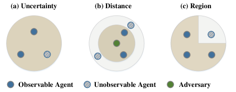
Partial observability is primarily attributed to three limitations (see Figure 1): (1) Uncertainty Limitation: This occurs when partial observability arises due to the constraints imposed by unpredictable environmental events. Examples include obstacle occlusion, noisy measurements, and sensor anomalies. (2) Distance Limitation: This refers to situations where the relative distance between agents exceeds their perceptual range, determined by the sensors deployed by MASs, such as LiDARs and millimeter-wave radars (Ren et al., 2019). (3) Region Limitation: Incomplete observations result from privacy concerns, security constraints, or rule restrictions, where specific boundaries define the region and could represent geographical areas or logical ranges. Examples in this regard encompass restricted areas due to permission controls or competitions with incomplete information, such as financial markets or Texas Hold’em poker.

This paper introduces SUB-PLAY, a novel black-box attack framework aimed at adversarial policy generation in partially observed multi-agent competitive environments. Our intuition lies in the divide-and-conquer principle, decomposing the attack into multiple subgames. Each subgame is then modeled as a partially observable stochastic game (POSG) (Littman, 1994), and MARL is employed to solve and obtain the corresponding subpolicy. Finally, we integrate all subpolicies in a hard-coded format to generate the ultimate adversarial policy. The attacker records the interactions at each time step in the form of transitions and allocates these transitions to a specific subgame replay buffer based on the observed number of victim agents. However, the number of transitions in each buffer is uneven due to varying probabilities of each subgame occurrence. This imbalance may lead to undertraining of some subpolicies. To mitigate this issue, we propose a transition dissemination mechanism that facilitates the sharing of transition from proximity subgames.

Extensive evaluation results demonstrate that SUB-PLAY can effectively address the aforementioned three partial observability limitations and outperform Victim-play in Predator-prey and World Communication, two representative multi-agent competitive environments open-sourced by OpenAI (Lowe et al., 2017). Compared to normal opponents, t-SNE analysis reveals a significant difference in the activations of the victim’s policy network during interactions with adversarial policies. Moreover, SUB-PLAY is algorithm-agnostic, i.e., applicable to both distributed and centralized MARL algorithms.

To explore strategies for mitigating adversarial policies, we evaluate three potential defenses. The results indicate that adversarial retraining is insufficient to counteract adversarial policies, while policy ensemble and fine-tuning could only moderately reduce the effectiveness of attacks. Nevertheless, insights from the evaluation suggest that defenders may mitigate security risks posed by adversarial policies through flexible deployment techniques. For example, periodically updating policies or increasing the diversity of policies in policy ensemble.

In summary, the paper makes the following contributions:

• To the best of our knowledge, SUB-PLAY is the first work to investigate the security threats of adversarial policies in multi-agent competitive environments, revealing that attackers can exploit vulnerabilities in the victim’s policy even with partial observations.

• We summarize three partially observable limitations and propose an observable-driven subgame construction method to accommodate these limitations.

• We conduct a systematic evaluation, demonstrating that SUB-PLAY outperforms the state-of-the-art attack framework ( Victim-play) in partially observable multi-agent competitive environments.

• We explore potential defenses, emphasizing that practitioners in MARL should not only focus on improving algorithm performance but also pay attention to deployment details, which is crucial in mitigating security threats posed by adversarial policies.

2. Background

2.1. Multi-Agent RL

MARL refers to scenarios where multiple agents are involved in sequential decision-making, and their policies are updated concurrently. This results in a non-stationary environment where the optimal policy for each agent changes over time, making the Markov property invalid (Sutton and Barto, 2018).

Figure 2. MARL training paradigms.

MARL Tasks. Based on the cooperation patterns among agents, MARL tasks are primarily divided into four categories: (1) Fully Cooperative MARL, where agents typically share a common reward function and collaborate to achieve a shared objective. Examples include multi-agent pathfinding and traffic management. (2) Fully Competitive MARL, where agents compete individually to outperform each other and pursue their objectives. These tasks are often modeled as two-player zero-sum Markov games, where cooperation between agents is impossible. Examples include Go or arm wrestling. (3) Self-interested MARL, where agents prioritize their benefits without considering others, as observed in domains like autonomous driving and stock trading. (4) Mixed MARL involves a blend of cooperative and competitive behavior. In most scenarios, two competing MASs exist, but agents within the same MAS collaborate. Examples include military exercises, multi-target encirclement, and team sports. The competitive environment discussed in this paper falls within a typical class of mixed MARL tasks.

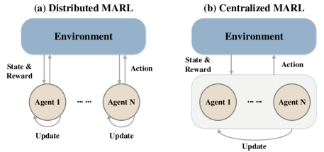
Training Paradigm. MARL has two training paradigms based on the presence or absence of a central decision-maker (Gronauer and Diepold, 2022). (1) Distributed MARL: The algorithms assume agents update policies independently, similar to single-agent implementations. Distributed Training Decentralized Execution (DTDE), a typical paradigm (e.g., independent Q-learning), allows efficient training and deployment without communication constraints. However, it may not be suitable for complex environments with many agents, as non-stationarity is neglected. (2) Centralized MARL: Centralized Training Centralized Execution (CTCE) is a centralized MARL paradigm with a centralized decision maker in training and deployment. It achieves theoretically optimal performance but needs communication guarantees and suffers from the curse of dimensionality (Nguyen et al., 2020). In contrast, Centralized Training Decentralized Execution (CTDE) algorithms, such as QMIX, MADDPG, and MAPPO, guide agents during training but enable independent decision-making during deployment without additional communication, offering state-of-the-art performance.

SUB-PLAY is not limited by the attacker’s communication capabilities or the number of agents under its control. Therefore, SUB-PLAY applies to both distributed and centralized MARL algorithms.

2.2. Adversarial Policy

The essence of adversarial policies lies in attackers leveraging RL technology to autonomously discover and exploit weaknesses and vulnerabilities within the RL policies deployed by victims. Existing research (Gleave et al., 2020; Wu et al., 2021; Guo et al., 2021; Wang et al., 2022) predominantly focuses on two-player competitions, assuming an attacker has the privilege to interact with a victim, can obtain a complete observation of the environment at each time step, and the victim fixedly deploys a well-trained policy.

The fundamental reason for the existence of adversarial policies stems from RL’s adoption of Self-play for policy training in competitive environments (Heinrich et al., 2015). However, Self-play cannot guarantee to reach a Nash equilibrium within finite training. In game theory, non-equilibrium policies are inevitably exploitable. Guided by this intuition, an attacker can manipulate its policy during training, updating it in a direction that maximizes the exploitation of the victim’s vulnerabilities.

For instance, while AlphaGo-style AIs outperform human champions, adversarial policies specifically trained against them still achieve a success rate of over 77% (Wang et al., 2022). Remarkably, these adversarial policies fall short when facing ordinary Go enthusiasts. This indicates that adversarial policies are highly targeted, sacrificing generalizability to intensify exploitation against a specific victim. Therefore, an adversarial policy is a complement to RL or a figuration of its weaknesses rather than a substitute.

Finding or approximating a Nash equilibrium in a multi-agent competition is at least as hard as PPAD-complete (Brown, 2020). This implies that in real deployment scenarios, MARL policies are exploitable. Therefore, MARL must be attentive to the potential risks posed by adversarial policies.

More details about the adversarial policy, including a more nuanced explanation of its existence and the upper limit of attack performance, can be found in Appendix A.

3. Threat Model and Problem Formulation

Figure 3. A two-team competitive environment can be simplified from a ZS-POSG to a POSG if the joint policy of $Victim$ is fixed.

3.1. Threat Model

In this paper, we propose an adversarial policy attack for mixed MARL tasks in two-team competitive environments.

Definition 1. A two-team competitive environment involves two MASs, Adversary and Victim, which consist of two sets of agents, $\mathcal{M}$ and $\mathcal{N}$, where $|\mathcal{M}|=$ M and $|\mathcal{N}|=$ N. Adversary and Victim are in full competition, while the agents within each MAS collaborate.

Attacker’s Goal. Maximizing the reduction of $Victim$’s performance on a specific MARL task.

Attacker’s Capabilities. The attacker possesses control over $Adversary$ and can update its MARL policy. Additionally, the attacker possesses interaction privileges with the $Victim$, obtaining partial observations about the environment at each time step. Apart from N, $Victim$ is regarded as a black box by the attacker. Moreover, the attacker is restricted from manipulating the environment.

We assume that $Victim$’s MARL policy is fixed, i.e., the parameters during the deployment phase are frozen (subsequent evaluations have indicated that this assumption can be relaxed). This is common for the deployment of RL on physical entities. For instance, a manufacturer releases an encirclement MAS consisting of multiple-legged robots (Fu et al., 2023a) or drones (Kaufmann et al., 2023). These physical entities fixedly deploy policies to avoid unacceptable losses due to exploration, such as robot malfunctions or drone crashes. Even if the manufacturer offers periodic policy upgrade services, the parameters of the MAS remain fixed between two consecutive updates, and this interval might span several months or even years. Once the attacker generates an adversarial policy, it implies that all users deploying the MAS from that manufacturer are exposed to the threat.

3.2. Problem Formulation

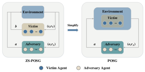
Based on the threat model, we formulate the attack as a zero-sum partially observable stochastic game (ZS-POSG) (Littman, 1994; Zhang et al., 2021; Hansen et al., 2004).

Figure 4. The framework of SUB-PLAY.

Definition 2. A zero-sum partially observable stochastic game is defined as

(1) $$\mathcal{G}=(\mathcal{S},\{\mathcal{A}^{i}\},\{\mathcal{B}^{j}\},\{\Omega^{i}\},\{\mathcal{O}^{i}\},\mathcal{P},\{\mathcal{R}_{A}^{i}\},\{\mathcal{R}_{V}^{j}\},\gamma),$$

where $\mathcal{S}$ denotes the state space, $\mathcal{A}^{i}$ (resp. $\mathcal{B}^{j}$) denotes the action space for agent $i\in\mathcal{M}$ (resp. $j\in\mathcal{N}$). $\mathcal{A}=\prod_{i\in\mathcal{M}}\mathcal{A}^{i}$ and $\mathcal{B}=\prod_{j\in\mathcal{N}}\mathcal{B}^{j}$ denote the joint action spaces for the adversary and the victim. Each agent $i\in\mathcal{M}$ receives an observation $o^{i}\in\Omega^{i}$, and the observation function $\mathcal{O}^{i}:\mathcal{S}\times\mathcal{A}\times\mathcal{B}\rightarrow\Delta(\Omega^{i})$ is a probability distribution over possible subsequent observations given the previous state and the actions of all agents. Each agent $j\in\mathcal{N}$ receives the global state $s\in\mathcal{S}$. $\mathcal{P}:\mathcal{S}\times\mathcal{A}\times\mathcal{B}\rightarrow\Delta(\mathcal{S})$ represents the probability that taking joint action $a\in\mathcal{A}$ and $b\in\mathcal{B}$ in state $s\in\mathcal{S}$ results in a transition to $s^{\prime}\in\mathcal{S}$. $\mathcal{R}_{A}^{i}:\mathcal{S}\times\mathcal{A}\times\mathcal{B}\rightarrow\mathbb{R}$ (resp. $\mathcal{R}_{V}^{j}:\mathcal{S}\times\mathcal{A}\times\mathcal{B}\rightarrow\mathbb{R}$) denotes the reward function for agent $i\in\mathcal{M}$ (resp. $j\in\mathcal{N}$). $\gamma\in[0,1)$ is the discount factor.

Let $\pi_{A}\in\mathbb{P}_{A}:\Omega\rightarrow\Delta(\mathcal{A})$ and $\pi_{V}\in\mathbb{P}_{V}:\mathcal{S}\rightarrow\Delta(\mathcal{B})$ be the joint policies of $Adversary$ and $Victim$, respectively. $\mathbb{P}_{A}$ and $\mathbb{P}_{V}$ are their corresponding joint policy spaces.

3.3. Problem Simplification

Inspired by (Guo et al., 2021), we define the following proposition (the proof is in Appendix B).

Proposition 1. In a zero-sum partially observable stochastic game, if the victim keeps a fixed joint policy $\pi_{V}$, the state transition of the environment is solely dependent on the adversary’s joint policy $\pi_{A}$.

According to Proposition 1, the attacker can treat $Victim$ as part of the environment (as shown in Figure 3) and simplify the attack from a ZS-POSG to a POSG:

(2) $$\mathcal{G}_{\alpha}=(\mathcal{S},\{\mathcal{A}^{i}\},\{\Omega^{i}\},\{\mathcal{O}_{\alpha}^{i}\},\mathcal{P}_{\alpha},\{\mathcal{R}_{\alpha}^{i}\},\gamma),$$

retains the same state space, action space for $Adversary$, observation space, and discount factor as the original $\mathcal{G}$. However, the observation function, transition function, and reward function for $Adversary$ are reconstructed as

(3) $$\mathcal{O}_{\alpha}^{i}(s,a)=\mathcal{O}^{i}(s,a,b),$$

$$\mathcal{P}_{\alpha}(s,a)=\mathcal{P}(s,a,b),$$

$$\mathcal{R}_{\alpha}^{i}(s,a)=\mathcal{R}_{A}^{i}(s,a,b),$$

where $a$ and $b$ are the joint actions of $Adversary$ and $Victim$, respectively. Eventually, the attacker’s objective translates into finding a policy $\pi_{A}\in\mathbb{P}_{A}$ that maximize the accumulated rewards $\sum_{i}^{M}\sum_{t=0}^{T}\gamma^{t}\mathcal{R}_{\alpha}^{i}(s_{t},a_{t})$ of $Adversary$.

4. Methodology

This section first introduces the framework of SUB-PLAY and then describes the design details of each step. The intuition behind SUB-PLAY is to adopt a divide-and-conquer strategy, decomposing a complex POSG, as depicted in Equation 2, into multiple relatively simpler POSGs. By tackling these simplified subgames individually, it becomes possible to address the overall complexity of the original POSG more efficiently.

Figure 5. The occupancy rate of subgames under three different limitations. The environment is Predator-prey, with $Victim$ consisting of three agents. The vertical coordinate contains the occupancy rate of four subgames $\{\mathcal{G}_{\alpha_{0}},\mathcal{G}_{\alpha_{1}},\mathcal{G}_{\alpha_{2}},\mathcal{G}_{\alpha_{3}}\}$. As time progresses, the attacker’s policy will be updated.

4.1. Attack Framework

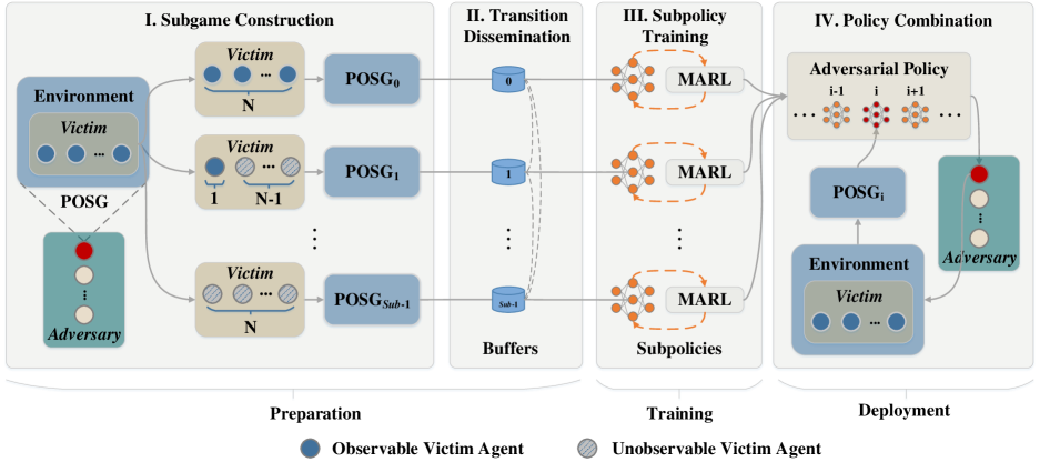
SUB-PLAY consists of four main steps: subgame construction, transition dissemination, subpolicy training, and policy combination (see Figure 4).

In the preparation phase, the attacker constructs multiple subgames based on the potentially observed number of victim agents and models each subgame as a POSG. Each subgame is a separate MARL problem, initializing its own subpolicy and replay buffers. For specific details of subgame construction, please refer to Section 4.2.

To mitigate the undertraining subpolicies caused by limited interaction transition, the attacker employs a uniform transition dissemination mechanism for all agents in $Adversary$. Then, each agent predefines a transition dissemination table, which is utilized to determine the probability of sharing each transition data among the replay buffers. For specific details of transition dissemination, please refer to Section 4.3.

In the training phase, $Adversary$ and $Victim$ interact within the environment. The generated transitions are stored in each replay buffer based on the probabilities determined in the transition dissemination table. When a replay buffer accumulates a batch of transitions, the MARL algorithm updates the corresponding subpolicy. The reward of $Adversary$ is negatively correlated with the performance of $Victim$ in the competition. Therefore, in accordance with the MARL paradigm, each subpolicy tends to minimize the performance of $Victim$ to achieve the attack objective. This reward-oriented process does not require any additional knowledge or human intervention. For specific details of subpolicy training, please refer to Section 4.4.

In the deployment phase, the attacker combines subpolicies to form an adversarial policy. Since the attacker has complete control over the adversary and stealthiness is not a concern, we implement the policy combination in a hard-coded manner. When launching an attack, $Adversary$ determines which subgame the current competition belongs to and then switches to the corresponding subpolicy to make decisions. More details of policy combination can be referred to Section 4.5.

4.2. Subgame Construction

For a partially observed MAS, the attacker constructs subgames based on the observed agents. We define

(4) $$\emph{Sub}=\emph{N}+1,$$

where Sub indicates the number of constructed subgames and $N$ is the number of agents belonging to $Victim$. All subgames form a set $\{\mathcal{G}_{\alpha_{k}}\}_{k\in\mathcal{K}}$. $\mathcal{K}$ = $\{0,1,...,\emph{Sub}-1\}$ and each subgame is fomulated as a POSG:

(5) $$\mathcal{G}_{\alpha_{k}}=(\mathcal{S},\{\mathcal{A}^{i}\},\{\Omega_{k}^{i}\},\{\mathcal{O}_{\alpha}^{i}\},\mathcal{P}_{\alpha},\{\mathcal{R}_{\alpha}^{i}\},\gamma),$$

where the only difference in this equation from Equation 2 is the term $\Omega_{k}^{i}\subseteq\Omega^{i}$. For example, if $Victim$ consists of two agents, the attacker constructs three subgames $\{\mathcal{G}_{\alpha_{0}},\mathcal{G}_{\alpha_{1}},\mathcal{G}_{\alpha_{2}}\}$, corresponding to the cases where the attacker observes 0, 1, and 2 agents from $Victim$, respectively.

Remark 1. In real-world environments, the partial information about specific agent components may be available to an attacker due to limited perspective. We propose that a conservative strategy can be adopted in high exploration cost environments, treating these agents as unobservable, while a more aggressive strategy can be employed in low exploration cost environments by treating them as observable.

Remark 2. Our method is scalable; for instance, the attacker could construct subgames based on regions or apply our method to scenarios where the victim is a single-agent system. In the latter case, subgames could be constructed based on the observability of different components of the single agent.

4.3. Transition Dissemination

The attacker records interactions with $Victim$ in the form of transitions. Each transition is represented as a tuple $(o_{t},a_{t},r_{t},o_{t+1})$, where $o_{t}$ is the observation at time step $t$, $a_{t}$ is the joint action of $Adversary$, $r_{t}$ is the instantaneous reward, $o_{t+1}$ is the observation at the next time step, and $t\in[0,T-1]$, where $T$ is the time horizon. Each agent in $Adversary$ maintains a set of replay buffers $\{\mathcal{E}_{k}^{i}\}$ that stores the transitions for each subgame, where $i\in\mathcal{M}$ denotes the agent’s identifier and $k\in\mathcal{K}$ denotes the subgame’s identifier.

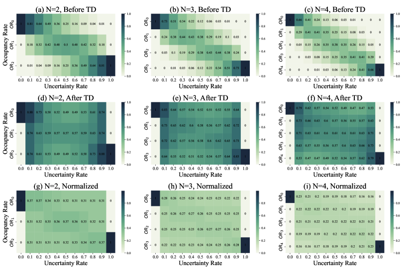
Empirical Study. We introduce a concept of Occupancy Rate (OR), which quantifies the occurrence frequency of a subgame. The occupancy rates are related to the number of transitions and serve as the foundation for constructing the transition dissemination table. We conduct an empirical study to explore the relationship between occupancy rates and three partially observable limitations (please refer to Section 5.1 for setup details). The results in Figure 5 reveal two key observations.

Observation 1. (Heterogeneity Property) The occupancy rate of subgames exhibit variations, which is further affected by the limitations of partial observability.

Using the first column of Figure 5(c) as an example, the occupancy rates for four subgames $\mathcal{G}{\alpha_{0}},\mathcal{G}{\alpha_{1}},\mathcal{G}{\alpha_{2}}$ and $\mathcal{G}{\alpha_{3}}$ are 0.04, 0.08, 0.24, and 0.65, respectively. The example highlights that some subgames, such as $\mathcal{G}{\alpha_{2}}$ and $\mathcal{G}{\alpha_{3}}$, occur frequently, leading to higher occupancy rates (0.24 and 0.65). These subgames provide a sufficient number of transitions, contributing to a more comprehensive dataset for learning and analysis. On the other hand, subgames like $\mathcal{G}{\alpha_{0}}$ and $\mathcal{G}{\alpha_{1}}$ occur infrequently, resulting in lower occupancy rates (0.04 and 0.08). The infrequent occurrence of these subgames leads to a scarcity of transitions, which may present challenges for effective learning and decision-making within those specific contexts.

Observation 2. (Dynamics Property) Under distance limitations, the occupancy rate of subgames is influenced by variations in the attacker’s policy.

The occupancy rates remain stable under uncertainty and region limitations, but they exhibit significant shifts under distance limitations. For example, OR₀ increases from 0.03 to 0.14, while OR₃ decreases from 0.57 to 0.35. The distance limitation is associated with an observable range represented by a circle centered around each agent in $Adversary$. Therefore, the observation by an agent is determined by its behavior pattern or policy.

The heterogeneity property underscores the non-uniform nature of occupancy rates across different subgames. We propose three methods aim to address this non-uniformity and determine occupancy rate values in such scenarios.

Static Estimation. Under uncertainty limitations, if we assume that the uncertainty in the observation of any $Victim$’s agent is the same, $OR_{k}$ is considered as the probability of repeatedly observing N agents in $Victim$ with exactly $k$ successes. The probability of successful observation is $\mu$, which can be introduced as priori knowledge or obtained from historical observation of $Victim$. Thus, the occupancy rate obeys a binomial distribution with parameters N and $\mu$, i.e.,

(6) $$OR_{k}=\tbinom{N}{k}\cdot\mu^{k}\cdot(1-\mu)^{N-k},$$

where $\tbinom{N}{k}$ is the binomial coefficient, which represents the number of ways to choose $k$ successes from $N$ trials.

Static Observation. Alternatively, the attacker calculates the occupancy rate for each subgame $\mathcal{G}_{\alpha_{k}}$ by counting the number of related transitions in all replay buffers.

(7) $$OR_{k}=\frac{|\mathcal{E}_{k}|}{|\mathcal{E}_{0}|+|\mathcal{E}_{1}|+...+|\mathcal{E}_{Sub-1}|},$$

where $|\mathcal{E}_{k}|=\sum_{i=1}^{M}|\mathcal{E}_{k}^{i}|$ and $|\mathcal{E}_{k}^{i}|$ indicates the number of transitions stored in $\mathcal{E}_{k}^{i}$. These transitions can either be direct interactions with $Victim$ or observations of $Victim$’s interactions with other MASs. Static observation does not rely on additional assumptions or prior knowledge and is applicable to all three types of limitations discussed in this paper.

Dynamic Observation. The dynamics property reveals that occupancy rates may exhibit significant fluctuations and migration in a competitive environment. To account for this, the attacker can utilize Exponentially Weighted Averages to accommodate the dynamics of occupancy rates:

(8) $$OR_{k_{t}}=\beta\cdot OR_{k_{t-1}}+(1-\beta)\cdot OR^{\prime}_{k_{t}},$$

where $OR_{k_{t-1}}$ denotes the current weighted average of $\mathcal{G}_{\alpha_{k}}$’s occupancy rate, $\beta$ denotes the weight of historical transition (e.g., $\beta$ = 0.9 means that the occupancy rate is approximately to the average of 10 episodes), and $OR^{\prime}_{k_{t}}$ denotes the occupancy rate obtained from the current episode statistics. Dynamic observation is applicable to all the three limitations and does not require additional assumptions or prior knowledge. Section 5.2 elucidates the strengths and weaknesses of these three methods through experiments and analysis, guiding on their selection.

Figure 6. Each agent in $Adversary$ maintains a transition dissemination table.

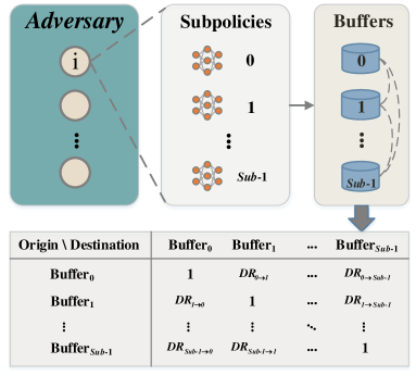
Transition Dissemination Table. The attacker determines the Dissemination Rate (DR) between each pair of replay buffers based on the occupancy rate. As shown in Figure 6, for each agent $i\in\mathcal{M}$, we define $DR_{\hat{k}\rightarrow k}\in[0,1]$ as the probability of transition transmission from buffer $\mathcal{E}^{i}_{\hat{k}}$ to buffer $\mathcal{E}_{k}^{i}$.

DRs are determined by a combination of four factors: (1) $DR_{\hat{k}\rightarrow k}$ is negatively correlated with the occupancy rate of the destination buffer $\mathcal{E}_{k}^{i}$ because the buffer with sufficient transitions does not require much additional transition. (2) $DR_{\hat{k}\rightarrow k}$ is negatively correlated with the distance between $\mathcal{G}_{\alpha_{\hat{k}}}$ and $\mathcal{G}_{\alpha_{k}}$, as transitions with higher similarity are provided between buffers close to each other. (3) $DR_{\hat{k}\rightarrow k}$ is positively correlated with the number of constructed subgames because the mean value of occupancy rates decreases as Sub increases. (4) $DR_{\hat{k}\rightarrow k}$ is negatively correlated with the dispersion of occupancy rates since high dispersion is prone to multiple occupancy rates with lower values. In summary, we define $DR_{\hat{k}\rightarrow k}$ as

(9) $$DR_{\hat{k}\rightarrow k}=\\ \begin{cases}\mathrm{clip}((\lambda-OR_{k}+\sigma)^{\frac{|\hat{k}-k|}{\sqrt{Sub}}},0,1),&\mathrm{if}\ OR_{k}\leq\lambda\\ \sigma^{\frac{|\hat{k}-k|}{\sqrt{Sub}}},&\mathrm{if}\ OR_{k}>\lambda\end{cases}$$

where $\lambda$ is an adjustment parameter positively correlated with the complexity of the two-team competitive environment. $\sigma$ is the standard deviation of all occupancy rates and is used to measure their dispersion. $|\hat{k}-k|$ indicates the distance between two subgames. $\sqrt{Sub}$ indicates that as the number of constructed subgames increases, the transition dissemination between buffers will become more frequent, meaning that the value of $DR_{\hat{k}\rightarrow k}$ will increase. We use the clip function to limit the value of $DR_{\hat{k}\rightarrow k}$ to the range [0,1].

All DRs collectively form a transition dissemination table. When a new transition is generated, the agent allocates it to various replay buffers based on the probabilities recorded in this table. If static estimation or static observation is employed to determine occupancy rates, this table is static. In contrast, if dynamic observation is used to determine occupancy rates, this table becomes dynamic. The impact of transition dissemination is presented in Figure 19 in the appendix.

Figure 7. The attack performance of SUB-PLAY under uncertainty limitations in Predator-prey.

4.4. Subpolicy Training

Each agent $i\in\mathcal{M}$ maintains a set $\{\pi_{\alpha_{k}}^{i}\}_{k\in\mathcal{K}}$ consisting of all subpolicies. We perform Policy Meritocracy (PM) to preserve top-performing subpolicies based on the harmonic mean of their test performance across $L$ metrics, mitigating performance fluctuations caused by non-stationarity.

(10) $$PM_{k}^{i}=\frac{L}{\sum\limits_{l=1}^{L}1/\eta_{k_{l}}^{i}},$$

where $\eta_{k_{l}}^{i}$ indicates the test performance of the subpolicy $\pi_{\alpha_{k}}^{i}$ with respect to metric $l$. In the policy pool, only one subpolicy is retained for each subgame to minimize storage overhead. Replacements occur when a subpolicy with superior test performance emerges. The detailed update process for the subpolicies is outlined in Algorithm 1 in the appendix.

4.5. Policy Combination

The attacker combines all subpolicies $\{\pi_{\alpha_{k}}^{i}\}_{i\in\mathcal{M},k\in\mathcal{K}}$ to generate the final adversarial policy. Specifically, at each time step of the deployment phase, $Adversary$ obtains a joint observation $(o_{1},o_{2},...,o_{M})$ and then outputs a joint action $(a_{1},a_{2},...,a_{M})$. The subgame construction ensures that each observation exclusively belongs to a single subgame, without any overlap or intersection between the subgames, i.e., $\Omega_{\hat{k}}^{i}\cap\Omega_{k}^{i}=\varnothing$, where $\hat{k}\neq k$ ($\hat{k},k\in\mathcal{K}$), $i\in\mathcal{M}$. Furthermore, unlike backdoor attacks (Goldblum et al., 2022; Wang et al., 2021a), the attacker can modify the program structure without concerns about stealthiness. Hence, we propose that the attacker can implement the policy combination in a hard-coded manner.

Taking the distributed MARL as an example, each agent $i\in\mathcal{M}$ determines which subgame a received observation $o_{i}$ belongs to and subsequently selects the corresponding subpolicy to guide its action decision-making:

(11) $$\pi_{\alpha}^{i}=\\ \begin{cases}\pi_{\alpha_{0}}^{i},&\mathrm{if}\ o_{i}\in\Omega_{0}^{i}\\ ...\\ \pi_{\alpha_{Sub-1}}^{i},&\mathrm{if}\ o_{i}\in\Omega_{Sub-1}^{i}\end{cases}$$

This approach has two advantages: it provides a straightforward logic and greater flexibility, allowing each subgame to employ a separate MARL algorithm. The implementation of policy combination can be found in Algorithm 2 in the appendix.

5. Evaluation

In this section, we first introduce the evaluation setup and then evaluate SUB-PLAY through four perspectives: attack performance, ablation study, transferability evaluation, and potential defenses.

5.1. Setup

Environment. We adopt two-dimensional environments, Predator-prey and World Communication, within the Multi Particle Environments (MPE) (Lowe et al., 2017) framework developed by OpenAI. MPE is a gym-based benchmark designed for cooperative, competitive, and mixed MARL tasks.

• Predator-prey. There are N slower predators controlled by $Victim$ and M preys controlled by $Adversary$. The predators cooperate to collide with preys, while the preys cooperate to avoid collisions. The environment is initialized randomly at the beginning of each episode, including the positions of agents and obstacles.

• World Communication. This environment shares similarities with the Predator-prey setup but includes additional features. (1) There are M foods that preys are rewarded for being close to. (2) The environment randomly initializes a forest, making all agents invisible within it initially. (3) A leader predator exists, having full visibility of all agents and the ability to communicate with other predators to enhance cooperation.

The state and action spaces of both environments are continuous. The evaluation of the attack performance is conducted in five different scenarios (MvN): 1v3, 2v3, 3v3, 2v2, and 4v2.

Figure 8. The attack performance of SUB-PLAY under distance limitations in Predator-prey.

Partial Observability Implementation. Observation is a multi-dimensional vector. We additionally introduce a Mask vector consisting of 0s and 1s, which has the same dimensions as Observation. The Mask is determined by specific rules for partial observability. We multiply each element of Observation with the corresponding element of the Mask, and the result is partial observation. For specific implementation, please consult Algorithm 3 in the appendix.

In Predator-prey, we conduct evaluations under both uncertainty and distance limitations. The uncertainty rate (i.e. $\mu$ in Equation 6) ranges from $\{0.00,0.25,0.50,0.75,1.00\}$. For example, $\mu=0$ indicates complete observability, and the mask array consists of all 1s. The observable distance ranges from $\{0.5,1.0,1.5,2.0\}$.

In World Communication, we conduct evaluations under region limitations. This environment has implemented partial observability, where agents located within a specific region are not visible (a forest with a fixed size but randomly initialized positions).

Implementation Details. Our evaluations are conducted on four servers with Intel(R) Xeon(R) CPU E5-2650 v4 @ 2.20GHz, 32GB RAM. Python and PyTorch are used for code implementation.

Selected MARL algorithms include DDPG and MADDPG, serving as representatives for DTDE and CTDE architectures, respectively. DDPG and MADDPG are actor-critic algorithms commonly used in reinforcement learning. These algorithms consist of an actor network and a critic network. We utilizes a two-layer ReLU MLP with 128 units in each layer to parameterize all policies. The actor network’s output layer incorporates a Tanh activation function. For weight initialization, we use Xavier normal with a gain of 1.0 for all layers in both victim and adversarial policy training. Biases are initialized with zeros. The chosen optimizer is Adam, with a learning rate of 0.001 and $\epsilon$ set to $10^{-8}$.

To ensure smooth policy updates, we employ Exponential Moving Average (EMA) with a decay rate of 0.95. Random noise sampled from a normal distribution with a standard deviation of 0.01 is added to the output actions to promote exploration. The discount factor $\gamma$ for RL is set to 0.95. The adjustment parameter $\lambda$ in Equation 9 is set to 0.5. All reported results are averaged over 1,000 test runs. For additional implementation details, parameter settings, and training results of $Victim$s, please refer to Appendix C.

Comparison Methods. (1) Baseline: $Victim$’s normal performance on a specific task. Specifically, $Adversary$ deploys a heuristic policy where the agent’s movement is characterized by a fixed speed and direction, with random updates after collisions. (2) Self-play (Bansal et al., 2018; Berner et al., 2019): Similar to the process of victim training, this setup grants the attacker complete access to the environment. The attacker randomly initializes both $Adversary$ and $Victim$, allowing them to compete with each other and undergo updates. Ultimately, $Adversary$ is retained to carry out the attack. (3) Victim-play (Gleave et al., 2020; Wu et al., 2021; Guo et al., 2021; Wang et al., 2022): Apart from substituting the algorithm with MARL, retain the other fundamental settings of this framework (refer to Section 2.2), specifically fixing $Victim$ and updating $Adversary$.

Metrics. We adopt Catch Rate (CR) and Collision Frequency (CF) as evaluation metrics.

(12) $$CR=\frac{Num_{c}}{Num_{e}},$$

where $\emph{Num}_{\emph{c}}$ indicates the number of episodes where the $Adversary$ is caught; $\emph{Num}_{\emph{e}}$ indicates the total number of episodes.

(13) $$CF=\frac{1}{Num_{e}}\sum_{e=1}^{Num_{e}}\sum_{j=1}^{N}Num_{ej},$$

where $\emph{Num}_{\emph{ej}}$ denotes the number of collisions between the jth predator and the prey in a specific episode e.

The attacker aims to evade pursuit and minimize $Victim$’s CR and CF. Policy meritocracy is based on the harmonic mean of these two metrics,

(14) $$PM=2\cdot\frac{CR\cdot CF}{CR+CF}.$$

We calculate the average improvement in attack performance of SUB-PLAY compared to Victim-play by

(15) $$\frac{(PM_{B}-PM_{S})-(PM_{B}-PM_{V})}{PM_{B}-PM_{V}},$$

where $PM_{B}$, $PM_{V}$, and $PM_{S}$ represent the victim’s average performance when the attacker executes Baseline, Victim-play, and SUB-PLAY, respectively.

Table 1. The impact of three occupancy rate determination methods on attack performance under three partial observability limitations. The performance is measured by two metrics (CR/CF). Acronyms: Static Estimation (SE), Static Observation (SO), Dynamic Observation (DO).

Limitations		DDPG			MADDPG
		SE	SO	DO	SE	SO	DO
Uncertainty	0.00	0.489 / 1.969	0.527 / 2.115	0.571 / 2.527	0.626 / 3.327	0.622 / 4.007	0.606 / 3.846
	0.25	0.401 / 1.573	0.538 / 2.205	0.575 / 2.532	0.579 / 3.053	0.607 / 3.506	0.725 / 6.460
	0.50	0.477 / 2.309	0.530 / 2.430	0.619 / 3.362	0.583 / 3.228	0.605 / 3.389	0.697 / 6.209
	0.75	0.502 / 1.927	0.532 / 2.395	0.580 / 2.475	0.591 / 3.318	0.614 / 3.909	0.639 / 3.904
	1.00	0.543 / 2.345	0.566 / 2.563	0.592 / 2.919	0.638 / 4.506	0.647 / 4.019	0.687 / 4.880
Distance	0.5	-	0.598 / 2.554	0.574 / 2.240	-	0.609 / 3.335	0.563 / 3.075
	1.0	-	0.657 / 3.059	0.571 / 2.529	-	0.647 / 4.148	0.614 / 3.500
	1.5	-	0.609 / 3.025	0.564 / 2.421	-	0.667 / 4.430	0.606 / 3.324
	2.0	-	0.620 / 2.786	0.561 / 2.579	-	0.654 / 4.464	0.589 / 3.264
Region	1	-	0.664 / 2.917	0.626 / 2.998	-	0.594 / 1.855	0.489 / 1.397

Figure 9. The attack performance of SUB-PLAY under region limitations in World Communication.

5.2. Attack Performance

We evaluate the attack performance of SUB-PLAY across different environments and limitations. The training process of SUB-PLAY can be found in Figure 16 in the appendix.

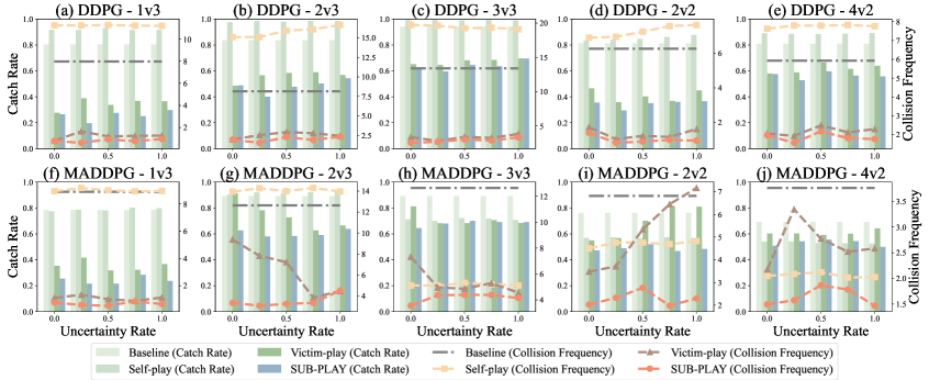
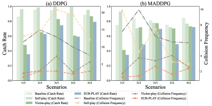
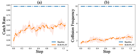
Under uncertainty limitations, SUB-PLAY, on average, reduces the victim’s performance to 51.98% of the baseline (see Figure 7). Moreover, SUB-PLAY outperforms the other two methods and minimizes the victim’s catch and collision rates in 94.0% (47/50) and 98.0% (49/50) scenarios. Compared to Victim-play, SUB-PLAY demonstrates an average improvement of 32.22% in attack performance (refer to Equation 15).

The results also show that when the MARL algorithm is MADDPG (resulting in increased input dimensionality due to information sharing among agents), SUB-PLAY demonstrates more stable attack performance, showcasing its potential to handle more complex environments. In addition, an unexpected outcome is that the attack remains effective even when the uncertainty is set to 1.00 (i.e., the attacker has no observations of the victim). According to Silver et al. (Silver et al., 2021), maximizing rewards is sufficient to drive intelligent behavior. In our scenarios, this suggests that the attacker can find adversarial policies by focusing on maximizing the rewards obtained, even without direct observation of the victim.

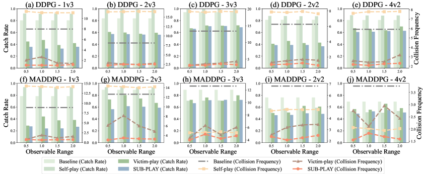
Under distance limitations, SUB-PLAY, on average, reduces the victim’s performance to 55.71% of the baseline (see Figure 8). Moreover, SUB-PLAY outperforms the other two methods and minimizes the victim’s catch and collision rates in 97.5% (39/40) scenarios. Compared to other methods, the impact of the observation range on SUB-PLAY is relatively minor, indicating that SUB-PLAY demonstrates better adaptability to dynamic environments. Compared to Victim-play, SUB-PLAY demonstrates an average improvement of 27.16% in attack performance.

Under region limitations, SUB-PLAY, on average, reduces the victim’s performance to 59.07% of the baseline (see Figure 9). Moreover, SUB-PLAY outperforms the other two methods and minimizes the victim’s catch and collision rates in 100.0% (10/10) scenarios. Compared to Victim-play, SUB-PLAY demonstrates an average improvement of 50.22% in attack performance.

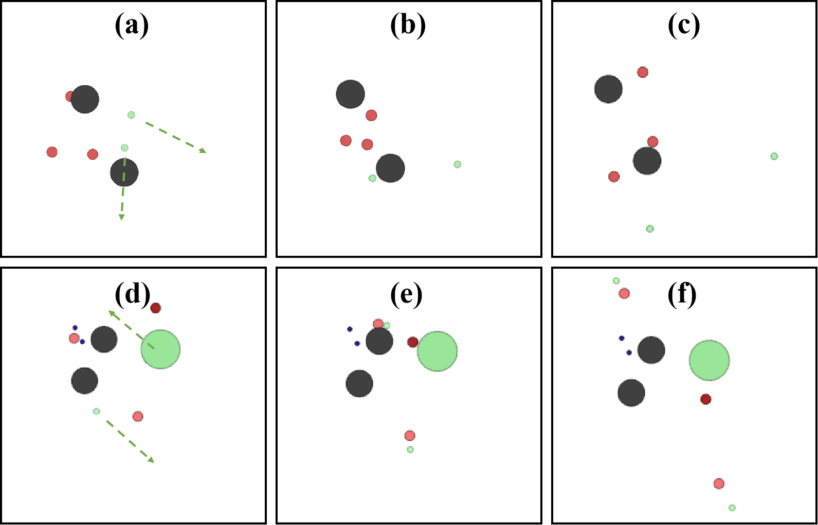
The visualization results (Figure 17 in the appendix) show that in Predator-prey, the preys tend to flee to the edge of the map at the maximum speed from different directions and then stay while trying to bypass predators and obstacles. They quickly get rid of collisions if they occur.

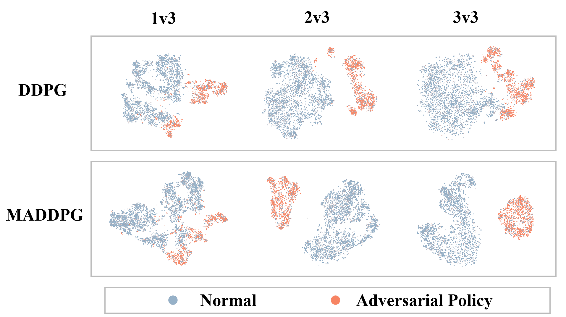
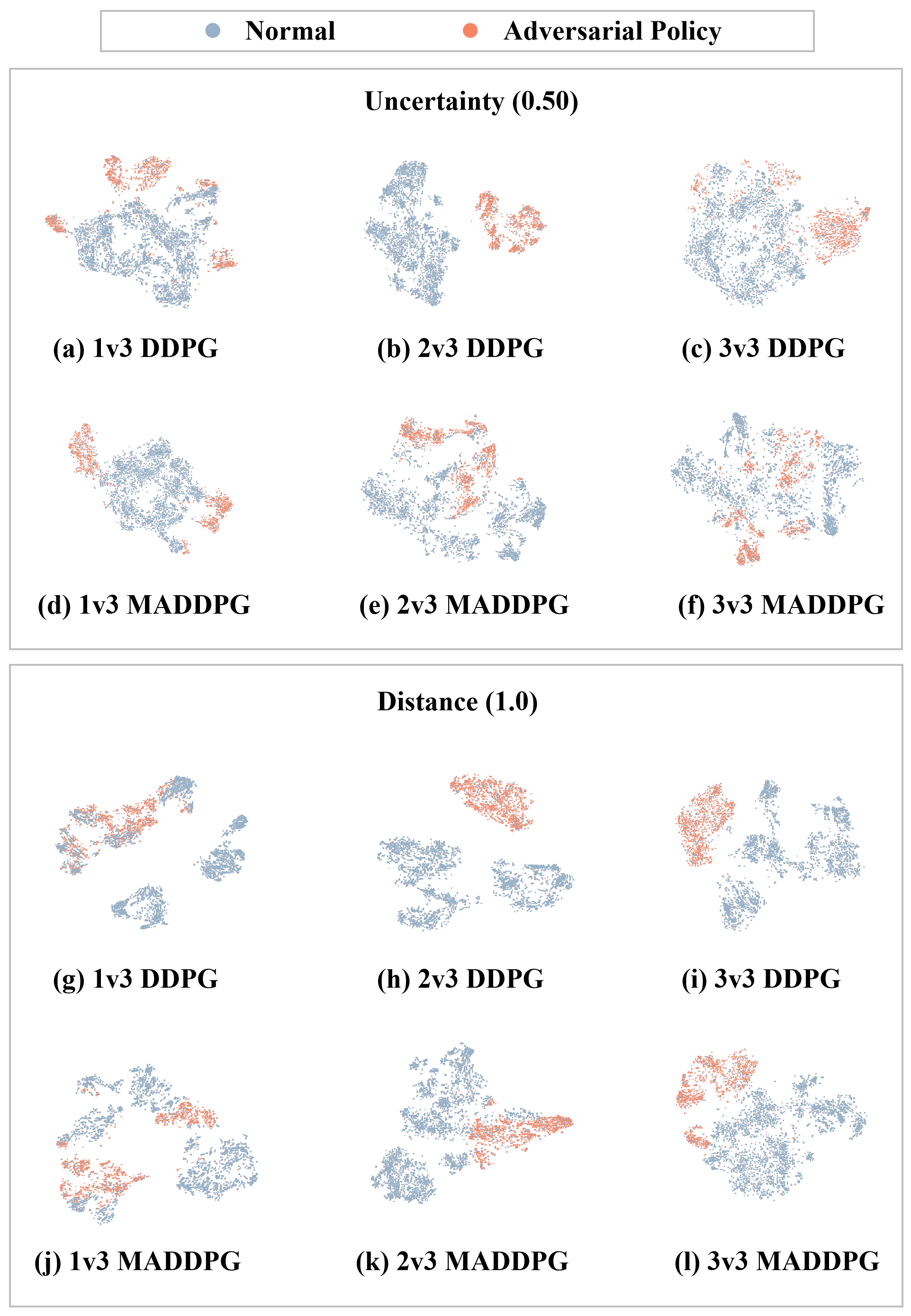
Similarly, in World Communication, the preys do not hide in the forest or approach foods for additional rewards. These observations demonstrate that adversarial policies effectively utilize the speed advantage of the preys to evade predators, mitigating the disadvantages of partial observability. t-SNE (see Figure 10) shows that the activations of the victim’s policy network are significantly different when facing a normal opponent compared to an adversarial policy. More results can be found in Figure 18 in the appendix.

Figure 10. t-SNE activations of the victim when playing against different opponents.

Table 2. The ablation results of components in SUB-PLAY measured by two metrics (CR/CF). Acronyms: Subgame Construction (SC), Transition Dissemination (TD), Policy Meritocracy (PM).

Methods	Limitations
	Uncertainty (0.25)	Uncertainty (0.50)	Distance (0.5)	Distance (2.0)	Region (1)
Self-play	0.920 / 14.280	0.916 / 13.998	0.936 / 14.349	0.935 / 14.187	0.704 / 4.486
Victim-play	0.782 / 7.823	0.727 / 7.215	0.728 / 6.163	0.670 / 4.891	0.718 / 3.763
SUB-PLAY (SC)	0.830 / 8.402	0.759 / 7.604	0.765 / 6.296	0.708 / 5.982	0.835 / 6.563
SUB-PLAY (SC+TD)	0.617 / 3.740	0.627 / 4.438	0.700 / 6.552	0.672 / 4.675	0.688 / 3.309
SUB-PLAY (SC+PM)	0.731 / 6.059	0.708 / 6.318	0.735 / 6.113	0.677 / 4.576	0.561 / 1.634
SUB-PLAY (SC+TD+PM)	0.579 / 3.053	0.583 / 3.228	0.563 / 3.075	0.589 / 3.264	0.489 / 1.397

Figure 11. The attack performance of subpolicies under uncertainty limitations.

Proactive Masking. Intuitively, partial observability poses a challenge for adversarial policy generation. However, evaluations indicate that proactive masking of environment observations may enhance the attack performance in some scenarios. For example, in Figure 7(a), the attack performance of SUB-PLAY is superior when the uncertainty rate is 0.25 compared to the fully observable scenario. The reason is that the minor partial observability corresponds to simplifying the input to the attacker. This suggests that proactive masking may facilitate early training of adversarial policies in complex environments. Recent work has introduced curriculum learning to address sparse rewards in adversarial policy generation (Wang et al., 2022), but it requires the access to different versions of victims. In contrast, proactive masking does not rely on a similar assumption.

Impact of Occupancy Rates. To compare the impact of the three methods proposed in Section 4.3 for determining occupancy rates, we evaluate them under three partial observability limitations (static estimation, static observation, and dynamic observation). In the static observation, the attacker pre-observes the victim for 1000 episodes, while in the dynamic observation, the parameter $\beta$ is set to 0.9.

Table 1 shows that SUB-PLAY achieves optimal attack performance with static estimation under uncertainty limitations. This is because static estimation provides more accurate occupancy rate estimations. Furthermore, SUB-PLAY performs superior attacks using dynamic observation under distance and region limitations. The former is due to the change in occupancy rates as the adversarial policy updates, while the latter is attributed to the additional dynamics introduced by the randomly initialized position of the forest in World Communication.

Therefore, in all evaluations, we set that the attacker adopts static evaluation under uncertainty limitations and dynamic observation under distance and region limitations.

5.3. Ablation Study

Unless additional specifications exist, the subsequent evaluations use the 2v3 scenario, and the MARL algorithm is set to MADDPG.

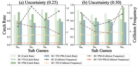
Component Evaluation. We perform an ablation study to assess the contribution of each component (subgame construction, transition dissemination, and policy meritocracy in subpolicy training) in SUB-PLAY. Table 2 demonstrates that when the subgame construction is applied in isolation, the performance of the adversarial policy is inferior. However, when transition dissemination is also performed, the attack performance of SUB-PLAY is significantly improved. This highlights the crucial role of transition dissemination in enhancing performance in partially observable environments. Policy meritocracy also contributes to improved attack performance and is compatible with subgame construction and transition dissemination.

Subgame Evaluation. We continue to explore the reasons behind the performance improvements achieved by SUB-PLAY. Figure 11 presents the attack performance of subpolicies in their respective corresponding subgames under uncertainty limitations. The results reveal that when the attacker only applies subgame construction and policy meritocracy, the resulting adversarial policies exhibit substantial performance differences across different subgames. However, with the inclusion of transition dissemination, all subpolicies show notable improvements in their attack performance. Furthermore, the performance disparities among the subpolicies are significantly reduced.

Figure 12. The transferability of adversarial policies across different scenarios. The vertical coordinate represents the limitation set in the training phase and the horizontal coordinate represents the limitation set in the testing phase.

Table 3. The attack performance of adversarial policies with heuristic victims. The performance is measured by two metrics (CR/CF).

Attaker		Heuristic	SUB-PLAY
Victim		Heuristic
Uncertainty	0.25	0.261 / 0.699	0.307 / 0.599
	0.50	0.259 / 0.694	0.286 / 0.515
Distance	0.5	0.225 / 0.613	0.275 / 0.508
	2.0	0.265 / 0.692	0.313 / 0.600
Region	1	0.304 / 0.802	0.439 / 0.807
Victim		MADDPG
Uncertainty	0.25	0.900 / 12.643	0.579 / 3.053
	0.50	0.918 / 13.258	0.583 / 3.228
Distance	0.5	0.942 / 13.540	0.563 / 3.075
	2.0	0.920 / 13.224	0.589 / 3.264
Region	1	0.837 / 9.954	0.489 / 1.397

5.4. Transferability

In real-world scenarios, the limitations on partial observability are not static; for instance, environmental factors like weather can impact sensor performance, leading to variations in the observable distance for the adversary agents. Therefore, we evaluate the transferability of adversarial policies across different parameter settings within the same limitation.

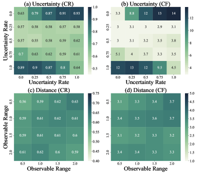
Figure 12(a)-(b) illustrate that adversarial policies can be transferred in specific scenarios (i.e., when the uncertainty rate is 0.25, 0.50, and 0.75). However, transferability diminishes when the uncertainty rate is 0.00 or 1.00. This is due to the significant differences in the modeling between fully unobservable and fully observable scenarios compared to partially observable scenarios. Additionally, subgame construction and transition dissemination are ineffective in these two cases. Figure 12(c)-(d) demonstrate that adversarial policies exhibit transferability under distance limitations. In conclusion, adversarial policies derived from SUB-PLAY demonstrate transferability in similar partially observable environments.

However, the transferability of adversarial policies encounters limitations when applied to victims with substantial differences. Table 3 illustrates that the adversarial policy proves ineffective in reducing the catch rate of heuristic victims, although it succeeds in diminishing their collision frequency. The reduction in collision frequency is attributed to the adversarial policy’s capacity to swiftly escape captures, whereas heuristic attackers frequently engage in repeated collisions. The inability to decrease the victims’ catch rate results from adversaries consistently moving at the maximum speed in the adversarial policy, thereby increasing the probability of collision – especially when preys are slow, potentially concluding the episode before colliding with predators. Moreover, preys lose the ability to evade nearby predators.

Figure 13. Adversarial retraining results of 5 rounds.

5.5. Potential Defenses

Adversarial policies pose significant challenges to the real-world deployment of MARL. In response, we explore viable defense approaches to mitigate these security threats.

Adversarial Retraining. An intuitive approach involves the victim adopting adversarial retraining during the training phase (Guo et al., 2023b). This allows the victim to identify and address vulnerabilities in its policy continuously. However, as shown in Figure 13, this does not render the adversarial policy ineffective. This is because there is no theoretical evidence indicates that the victim’s MARL policy, after adversarial retraining, can approach a Nash equilibrium more closely. Thus, the exploitable space persists, albeit potentially shifting with adversarial retraining. Moreover, as previously mentioned, finding or approximating a Nash equilibrium in a multi-agent competition is at least as tricky as PPAD-complete.

Policy Ensemble. While it is challenging to eliminate the threat posed by adversarial policies through training alone, victims could mitigate this threat by adjusting MARL’s deployment strategy. One such strategy involves adopting a policy ensemble approach, where the victim prepares a set of policies and consistently selects policies from this ensemble for deployment. Intuitively, this may prevent the attacker from adapting to a specific policy.

The results on the left side of Table 4 indicate that if attackers have access to all policies, the policy ensemble shows limited defensive effect. For instance, the entry in the first row and first column, -0.07, denotes a decrease of 0.07% in the effectiveness of adversarial policies, which is almost negligible (note that -100% corresponds to the failure of the adversarial policy). This implies that the assumption of freezing the victim’s policy in Section 3.1 can be relaxed.

If attackers have access to only a subset of the victim’s policies (33%), there is a certain degree of reduction in the effectiveness of adversarial policies (the results on the right side of Table 4). The insight derived from this is that the victim could periodically update the ensemble pool to prevent the attacker from adapting to all policies. The victim may also consider increasing the diversity of the policies in the pool (Fu et al., 2023b; Henderson et al., 2018), making their weaknesses significantly different, which might lead to fluctuations in adversarial policies, preventing them from converging. Policy ensemble can be coupled with a dynamic switching mechanism to enhance the defense approach further, wherein the switching time or policy selection is dynamically changed.

Victim Fine-tuning. Continual fine-tuning during deployment may also prevent the attacker from adapting to a specific victim, offering lower training costs than policy ensemble. However, the limited defensive effectiveness of fine-tuning, as shown in Figure 14, suggests that the distance between policies before and after fine-tuning remains close.

Table 4. The defensive effectiveness of policy ensemble, with values given in percentage (%).

Access	100%			33%
Scenarios	1v3	2v3	3v3	1v3	2v3	3v3
Uncertainty
0.00	-0.07	+0.02	-0.04	-2.74	+4.09	-0.89
0.25	+0.02	-0.25	+0.10	-9.86	-13.58	-12.45
0.50	+0.00	-0.02	+0.08	-9.68	-9.14	-17.01
0.75	-0.01	-0.07	+0.04	-15.55	-2.56	+2.85
1.00	+0.00	+0.04	+0.08	-25.78	-0.55	+9.68
Distance
0.5	-0.09	-0.15	-0.03	-16.17	-7.99	-11.98
1.0	-0.12	-0.12	-0.01	-30.15	-5.65	+0.25
1.5	-0.29	-0.12	-0.02	-20.24	-9.36	-32.69
2.0	-0.13	-0.28	+0.14	-16.01	-20.51	-43.39
Region
1	-0.08	-0.24	+0.00	-7.99	-37.44	-17.94

6. Discussion

Emphasizing Deployment Details. We not only introduce SUB-PLAY but also reveal that even with partial observations, adversarial policies induce the failure of MARL. Since mitigating the threat of adversarial policies through improvements in the training framework is challenging, we propose that defenders prioritize the deployment details of MARL rather than solely focusing on enhancing algorithm performance. Additionally, SUB-PLAY can serve as a method to measure the lower bound of MARL performance in adversarial scenarios.

Limitation and Future Work. SUB-PLAY still has some limitations. (1) Due to the scarcity of environments that facilitate multi-agent competitive settings with partial observability, our testing is limited to two environments. However, we extensively evaluate SUB-PLAY in various settings, including different types of partial observability limitations, multiple scenarios with varying numbers of agents, and two MARL architectures. (2) Although no additional interaction is required, the computational overhead incurred by SUB-PLAY is directly proportional to the number of subgames. Thus, a trade-off exists between computational overhead and attack performance, which remains challenging to address. (3) The current method assumes that the attacker engages in multiple interactions with the victim. We plan to adopt offline or batch-based RL techniques (Levine et al., 2020) to relax this setup.

Figure 14. The attack performance varies with the fine-tuning of the victim’s policy.

7. Related Work

7.1. RL Security

A substantial body of research is leveraging RL to achieve specific security objectives  (Wang et al., 2021b; Gohil et al., 2022; Yu et al., 2023; Maiti et al., 2023; Xia et al., 2023). Nevertheless, the security dimensions inherent to RL need to be more adequately addressed. This section thoroughly examines security research concerning the three fundamental components of RL.

Reward Manipulation. Unlike the modification of labels in deep learning (Wang et al., 2019; Yao et al., 2019), RL introduces backdoor attacks via reward manipulation (Ma et al., 2019; Kiourti et al., 2020). Zhang et al. (Zhang et al., 2020) developed a dynamic reward-poisoning attack targeting online RL applications, while Chen et al. (Chen et al., 2022) extended the concept of backdoor attacks to cooperative MASs. Wang et al. (Wang et al., 2021a) introduced a unique RL-specific paradigm for backdoor attacks, where the attacker trains a benign policy and a trojan policy, merging them into a backdoor policy by behavior cloning. Guo et al. (Guo et al., 2023a) discovered a pseudo-trigger space that can trigger RL backdoors. In response, they proposed PolicyCleanse to perform model detection and backdoor mitigation.

State Manipulation. Inspired by adversarial examples (Carlini and Wagner, 2017; Yu et al., 2020; Li et al., 2020), attackers in RL can disrupt the victim by perturbing the environment state. Huang et al. (Huang et al., 2017) applied FGSM (Goodfellow et al., 2015) to DRL and launched an adversarial attack on the DQN policy in Atari games (Mnih et al., 2015). Behzadan et al. (Behzadan and Munir, 2017) introduced a policy induction attack, where the attacker determines the victim’s actions based on a pre-trained target policy and perturbs the states by FGSM and JSMA (Papernot et al., 2016). Sun et al. (Sun et al., 2020) proposed a white-box attack called the critical point attack, which strategically explores state-action combinations to identify points with high payoff and inject subtle perturbations during the victim’s deployment phase.

Action Manipulation. The agent’s action determines the agent-environment boundary, allowing attackers to launch attacks by manipulating it. Lee et al. (Lee et al., 2020) proposed two victim manipulation attacks: the myopic action-space attack injects action perturbations based on current observations, while the look-ahead action-space attack considers future steps to maximize the attack’s impact. However, directly manipulating the victim’s actions is impractical.

In contrast, adversarial policies only need to control the attacker’s action. Gleave et al. (Gleave et al., 2020) pioneered Victim-play, which involves manipulating the adversary’s actions to induce suboptimal decisions from a fixed RL model during deployment. Wu et al. (Wu et al., 2021) incorporated explainable AI techniques into adversarial policy generation, enhancing stealthiness by launching attacks only when the victim pays attention to them. Guo et al. (Guo et al., 2021) extended Victim-play from zero-sum to general-sum environments, revealing its potential in assessing the fairness of competitions or systems. Wang et al. (Wang et al., 2022) explored adversarial policies in discrete action scenarios and achieved success against superhuman-level Go AIs, demonstrating that near-Nash or $\epsilon\emph{-equilibrium}$ policies are exploitable. Guo et al. (Guo et al., 2023b) attempted to mitigate the potential threat of adversarial policies from a training perspective and introduced a provable defense called PATROL. The aim is to bring the victim closer to a Nash equilibrium in a two-player competition.

7.2. Partial Observability in RL

Partial observability limits the attacker’s access to complete environmental information. To address this, existing research suggests two potential methods for the attacker.

Inference. Inference entails using available observations and prior knowledge to complete unobserved content, including environmental (Yang et al., 2021; Xu et al., 2022) and agent inference (Papoudakis et al., 2021; Gu et al., 2022). (1) Environmental Inference: Partial state information is used to infer the global environment in the spatial dimension. Yang et al. (Yang et al., 2021) proposed a supervised learning-based hallucinator for inferring the environment from current observations, effective in static environments but potentially less suitable for highly dynamic competitions. (2) Agent Inference: Historical interaction is used to infer the unobservable agents in the temporal dimension. Papoudakis et al. (Papoudakis et al., 2021) proposed constructing policies for all agents through representation learning. During deployment, the policies and local observations of the controlled agent are utilized to infer the invisible agents. However, this method relies on the victim’s policy knowledge and is unsuitable for black-box or competitive environments.

Generalization. Enhancing the generalization capability of agents can effectively adapt to the environment’s diversity, dynamics, and unpredictability (Kirk et al., 2023). Intuitively, this also applies to policy improvements in partially observable scenarios. Ghosh et al. (Ghosh et al., 2021) demonstrated that partitioning a partially observable task into multiple subtasks can effectively improve the performance of RL policies. SUB-PLAY draws on the insight of generalization-based approaches to address the partially observable problem in two-team competitive environments, as it applies to dynamic environments and does not rely on additional victim information.

8. Conclusion

This paper proposes SUB-PLAY, a novel black-box attack framework in partially observable two-team competitive environments. The effectiveness of SUB-PLAY in enhancing the attack performance of adversarial policies is showcased through divide-and-conquer strategies and transition dissemination, as evidenced by extensive evaluations conducted across various partially observable limitations and MARL algorithms.

Appendix A Exploitable Ceiling

In a ZS-POSG, an adversarial policy can be interpreted as an exploitative strategy akin to the strategies used in competitions like Texas Hold’em poker (Brown and Sandholm, 2019). Exploitative strategies capitalize on opponents’ vulnerabilities or tendencies, diverging from strict adherence to optimal or equilibrium strategy. Additionally, it’s essential to note that real-world competitions, such as military conflicts, often lack the same level of well-defined rules and fairness seen in games like Texas Hold’em poker. This implies that one of the MAS, whether the adversary or the victim, can benefit from the vulnerabilities in the competition rules. Therefore, the attack performance of an adversarial policy relies on the victim’s policy and the competition rule, with an upper bound referred to as the exploitable ceiling.

Definition 3. Exploitable ceiling refers to the limit of the performance degradation of the victim’s policy in a specific competitive environment, which is formalized as

(16) $$\mathcal{C}=\mathcal{C}(\pi_{V})+\mathcal{C}(e),$$

where $\mathcal{C}(\pi_{V})$ denotes the exploitable ceiling of the victim’s policy and $\mathcal{C}(e)$ denotes the exploitable ceiling of a two-team competitive environment.

The specific measurement of the exploitable ceiling could be approached from both the perspectives of the victim and the adversary. Considering the victim’s deployed policy $\pi_{V}$ and assuming that the victim possesses a Nash equilibrium policy $\pi_{V}^{*}$ in the constructed POSG, the exploitable ceiling can be defined as the victim’s regret:

(17) $$\mathcal{C}=\max\limits_{\pi_{V}^{*}\in\mathbb{P}_{V}}R(\pi_{V},\pi_{V}^{*}),$$

where $\pi_{V}^{*}$ denotes a Nash equilibrium policy of the victim in the environment. $R(\pi_{V},\pi_{V}^{*})$ denotes the expected regret of policy $\pi_{V}$ against $\pi_{V}^{*}$, which is defined as:

(18) $$R(\pi_{V},\pi_{V}^{*})=\mathbb{E}[\sum_{t=0}^{T}(r_{t}(\pi_{V},b_{t})-r_{t}(\pi_{V}^{*},b_{t}^{*}))],$$

where $r_{t}$ is the reward received by the victim at time $t$, $b_{t}$ is the action taken by policy $\pi_{V}$ at time $t$, $b_{t}^{*}$ is the action taken by $\pi_{V}^{*}$ at time $t$, and $T$ is the time horizon.

However, the existence of a Nash equilibrium is not guaranteed in a ZS-POSG due to an expanded policy space and challenges from incomplete information. In such cases, the exploitable ceiling can be defined as the adversary’s best response to the policy $\pi_{V}$:

(19) $$\mathcal{C}=\max\limits_{\pi_{A}\in\mathbb{P}_{A}}\mathbb{E}[u(\pi_{A}^{\prime},\pi_{V})-u(\pi_{A},\pi_{V})],$$

where $\pi_{A}^{\prime}$ denotes the adversary’s initial policy. $u(\pi_{A}^{\prime},\pi_{V})$ is the adversary’s utility function, denoting the expected accumulated reward when the adversary adopts $\pi_{A}^{\prime}$ to compete with $\pi_{V}$. Similarly, $u(\pi_{A},\pi_{V})$ denotes the expected accumulated reward when the adversary adopts an arbitrary $\pi_{A}\in\mathbb{P}_{A}$ to compete with $\pi_{V}$.

Appendix B Proof of Proposition 1

Proposition 1. In a zero-sum partially observable stochastic game, if the victim keeps a fixed joint policy $\pi_{V}$, the state transition of the environment is solely dependent on the adversary’s joint policy $\pi_{A}$.

Proof. The transition probability to $s_{t+1}$ under the state $s_{t}$ and the joint actions $(a_{t},b_{t})$ is

$$P(s_{t+1},a_{t},b_{t}|s_{t}) =P(s_{t+1}|a_{t},b_{t},s_{t})P(a_{t},b_{t}|s_{t})$$

$$=P(s_{t+1}|a_{t},b_{t},s_{t})P(a_{t}|b_{t},s_{t})\pi_{V}(b_{t}|s_{t}),$$

where $\pi_{V}$ is a fixed joint policy deployed by $Victim$. Therefore, $\pi_{V}(b_{t}|s_{t})$ can be replaced by a constant $c$ as

$$P(s_{t+1},a_{t},b_{t}|s_{t}) =c\cdot P(s_{t+1}|a_{t},b_{t},s_{t})P(a_{t}|b_{t},s_{t})$$

$$=c\cdot P(s_{t+1}|a_{t},b_{t},s_{t})\pi_{A}(a_{t}|s_{t}),$$

where

$$\pi_{A}(a_{t}|s_{t})=\pi_{A}(a_{t}|o_{t})P(o_{t}|s_{t},a_{t-1},b_{t-1}).$$

In our assumption, all agents make decisions simultaneously. Therefore, the joint action of $Adversary$ at time $t$ is only dependent on the state $s_{t}$, represented as $P(a_{t}|b_{t},s_{t})=\pi_{A}(a_{t}|s_{t})$. $s_{t}$ in $\pi_{A}(a_{t}|s_{t})$ is replaced with $o_{t}$ since $Adversary$ can only obtain partial observations. In the derivation, the joint policy $\pi_{A}$ is the only component that changes as the attacker refines their adversarial policy.

Further, given a set of trajectories $\{\tau_{1},...,\tau_{K}\}$, the state-value function of $Adversary$ can be defined as

$$V_{\pi_{A}}=\sum_{i=0}^{M}\sum_{k=0}^{K}\mathcal{R}_{A}^{i}(\tau_{k})P(\tau_{k}),$$

where

$$P(\tau) =P(s_{0})\prod_{t=1}^{T}P(s_{t},a_{t-1},b_{t-1}|s_{t-1})$$

$$=P(s_{0})\prod_{t=1}^{T}P(s_{t},a_{t-1}|b_{t-1},s_{t-1})\pi_{V}(b_{t-1}|s_{t-1})$$

$$=P(s_{0})\prod_{t=1}^{T}c\cdot P(s_{t},a_{t-1}|b_{t-1},s_{t-1})$$

$$=P(s_{0})\prod_{t=1}^{T}c\cdot P(s_{t}|a_{t-1},b_{t-1},s_{t-1})\pi_{A}(a_{t-1}|s_{t-1}),$$

where $T$ denotes the time horizon and

$$\pi_{A}(a_{t-1}|s_{t-1})=\pi_{A}(a_{t-1}|o_{t-1})P(o_{t-1}|s_{t-1},a_{t-2},b_{t-2}).$$

The joint policy $\pi_{A}$ is the only component that undergoes changes during adversarial policy training, similar to the transition probability. Furthermore, it can be shown that $\pi_{A}$ is also the only component that changes in the state-value function of $Adversary$. In summary, the state transition and state-value functions of the ZS-POSG depend solely on the modifications made to $\pi_{A}$ while keeping the joint policy $\pi_{V}$ of $Victim$ fixed.

Figure 15. The training curves of victims in diverse scenarios.

Figure 16. The variation in attack performance of adversarial policies.

Algorithm 1 Subpolicy Training.

1:  Input: $Adversary$’s latest subpolicies $\{\pi_{\alpha_{k}}^{i}\}_{i\in\mathcal{M},k\in\mathcal{K}}$, replay buffers $\{\mathcal{E}_{k}^{i}\}_{i\in\mathcal{M},k\in\mathcal{K}}$, and recorded test performance $\{PM_{k}^{i}\}_{i\in\mathcal{M},k\in\mathcal{K}}$.

2:  for $i=1,2,...,M$ do

3:   for $k=0,1,...,\emph{Sub}-1$ do

4:    Randomly select a batch of transitions from $\mathcal{E}_{k}^{i}$.

5:    Obtain $\overline{\pi}_{\alpha_{k}}^{i}$ through MARL training.

6:    Test the performance of $\overline{\pi}_{\alpha_{k}}^{i}$ on each metric and record it as $\{\eta_{k_{0}}^{i},\eta_{k_{1}}^{i},...,\eta_{k_{L}}^{i}\}$.

7:    Calculate $\overline{PM}_{k}^{i}$ by Equation 10.

8:    if $\overline{PM}_{k}^{i}$ outperforms $PM_{k}^{i}$ then

9:     $\pi_{\alpha_{k}}^{i}\leftarrow\overline{\pi}_{\alpha_{k}}^{i}$, $PM_{k}^{i}\leftarrow\overline{PM}_{k}^{i}$

10:    end if

11:   end for

12:  end for

13:  Output: Updated $\{\pi_{\alpha_{k}}^{i}\}_{k\in\mathcal{K},i\in\mathcal{M}}$ and $\{PM_{k}^{i}\}_{k\in\mathcal{K},i\in\mathcal{M}}$

Algorithm 2 Policy Combination (Distributed MARL Version).

1:  Input: $Adversary$’s joint observation $(o_{1},o_{2},...,o_{M})$, the constructed subgames $\{\mathcal{G}_{\alpha_{k}}\}_{k\in\mathcal{K}}$, the set $\{\pi_{\alpha_{k}}^{i}\}_{k\in\mathcal{K},i\in\mathcal{M}}$ consisting of all subpolicies.

2:  for $i=1,2,...,M$ do

3:   for $k=0,1,...,\emph{Sub}-1$ do

4:    if $o_{i}\in\Omega_{k}^{i}$ then

5:     $a_{i}\leftarrow\pi_{\alpha_{k}}^{i}(o_{i})$

6:    end if

7:   end for

8:  end for

9:  Output: $Adversary$’s joint action $(a_{0},a_{1},...,a_{M})$.

Algorithm 3 Partially Observable Implementation.

1:  Input: The joint state provided by the environment $(s_{1},s_{2},...,s_{M})$, the partially observable limitation $\mathcal{L}$.

2:  for $i=1,2,...,M$ do

3:   if $\mathcal{L}=$ Uncertainty Limitation then

4:    Generate a mask vector $m_{u}$ based on the uncertainty rate.

5:    $o_{i}\leftarrow s_{i}\odot m_{u}$

6:   end if

7:   if $\mathcal{L}=$ Distance Limitation then

8:    Generate a mask vector $m_{d}$ based on the observable distance.

9:    $o_{i}\leftarrow s_{i}\odot m_{d}$

10:   end if

11:   if $\mathcal{L}=$ Region Limitation then

12:    $o_{i}\leftarrow s_{i}$

13:   end if

14:  end for

15:  Output: Modified joint observation $(o_{0},o_{1},...,o_{M})$.

Figure 17. The visualization of adversarial policies. (a)-(c) are visualizations of one episode in Predator-prey. (d)-(f) are visualizations of one episode in World Communication.

Figure 18. More t-SNE results. Model fitted with a perplexity of 250 to activations from 5000 timesteps against each opponent.

Appendix C Additional Implementation Details

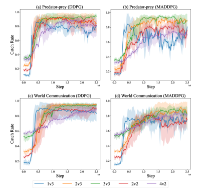
Victim Training. $Victim$s are derived from Self-play, which is a general framework in RL competitive environments (Bansal et al., 2018). Each victim is equipped with a replay buffer of size 200,000 and a batch size of 1024. Throughout the training phase, the victims undertake 100,000 episodes, which corresponds to 2,500,000 steps. To account for variations, we train three victims for every scenario, each initialized with a different random seed. The training progress of these victims is illustrated in Figure 15.

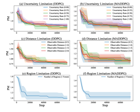
Adversarial Policy Generation. During the attack phase, each adversary agent utilizes a replay buffer with a size of 512 and a batch size of 512. Similar to the victim agents, we train three separate adversarial policies with different random seeds for each victim. The training curves of these adversarial policies can be observed in Figure 16. Notably, the victim agents require an average of 700,000 steps to converge, whereas the adversarial policies achieve convergence in only approximately 20,000 steps (compare Figure 15 and Figure 16). These results indicate a notable disparity in the convergence rates between the victim and adversary.

Figure 19. The occupancy rate of transitions for each replay buffer in different environments under uncertainty limitations. (a)-(c) denote the cases without transition dissemination; (d)-(f) denote the cases with transition dissemination; (g)-(i) denote the normalized result of occupancy rate after transition dissemination.

References

- (1)
- Bansal et al. (2018) Trapit Bansal, Jakub Pachocki, Szymon Sidor, Ilya Sutskever, and Igor Mordatch. 2018. Emergent complexity via multi-agent competition. International Conference on Learning Representations (2018).
- Behzadan and Munir (2017) Vahid Behzadan and Arslan Munir. 2017. Vulnerability of deep reinforcement learning to policy induction attacks. In International Conference on Machine Learning and Data Mining in Pattern Recognition. Springer, 262–275.
- Berner et al. (2019) Christopher Berner, Greg Brockman, Brooke Chan, Vicki Cheung, Przemysław Dębiak, Christy Dennison, David Farhi, Quirin Fischer, Shariq Hashme, Chris Hesse, et al. 2019. Dota 2 with large scale deep reinforcement learning. arXiv preprint arXiv:1912.06680 (2019).
- Brown (2020) Noam Brown. 2020. Equilibrium finding for large adversarial imperfect-information games. PhD thesis (2020).
- Brown and Sandholm (2019) Noam Brown and Tuomas Sandholm. 2019. Superhuman AI for multiplayer poker. Science 365, 6456 (2019), 885–890.
- Carlini and Wagner (2017) Nicholas Carlini and David Wagner. 2017. Towards evaluating the robustness of neural networks. In 2017 IEEE Symposium on Security and Privacy (S&P). IEEE, 39–57.
- Chen et al. (2022) Yanjiao Chen, Zhicong Zheng, and Xueluan Gong. 2022. MARNet: Backdoor Attacks Against Cooperative Multi-Agent Reinforcement Learning. IEEE Transactions on Dependable and Secure Computing (2022).
- Fernandez et al. (2021) Rolando Fernandez, Derrik E Asher, Anjon Basak, Piyush K Sharma, Erin G Zaroukian, Christopher D Hsu, Michael R Dorothy, Christopher M Kroninger, Luke Frerichs, John Rogers, et al. 2021. Multi-agent coordination for strategic maneuver with a survey of reinforcement learning. Technical Report. US Army Combat Capabilities Development Command, Army Research Laboratory.
- Fu et al. (2023b) Wei Fu, Weihua Du, Jingwei Li, Sunli Chen, Jingzhao Zhang, and Yi Wu. 2023b. Iteratively Learn Diverse Strategies with State Distance Information. In Thirty-seventh Conference on Neural Information Processing Systems.
- Fu et al. (2023a) Zipeng Fu, Xuxin Cheng, and Deepak Pathak. 2023a. Deep whole-body control: learning a unified policy for manipulation and locomotion. In Conference on Robot Learning. PMLR, 138–149.
- Ghosh et al. (2021) Dibya Ghosh, Jad Rahme, Aviral Kumar, Amy Zhang, Ryan P Adams, and Sergey Levine. 2021. Why generalization in rl is difficult: Epistemic pomdps and implicit partial observability. Advances in Neural Information Processing Systems 34 (2021), 25502–25515.
- Gleave et al. (2020) Adam Gleave, Michael Dennis, Cody Wild, Neel Kant, Sergey Levine, and Stuart Russell. 2020. Adversarial policies: Attacking deep reinforcement learning. International Conference on Learning Representations (2020).
- Gohil et al. (2022) Vasudev Gohil, Hao Guo, Satwik Patnaik, and Jeyavijayan Rajendran. 2022. ATTRITION: Attacking Static Hardware Trojan Detection Techniques Using Reinforcement Learning. In Proceedings of the 2022 ACM SIGSAC Conference on Computer and Communications Security. 1275–1289.
- Goldblum et al. (2022) Micah Goldblum, Dimitris Tsipras, Chulin Xie, Xinyun Chen, Avi Schwarzschild, Dawn Song, Aleksander Mądry, Bo Li, and Tom Goldstein. 2022. Dataset security for machine learning: Data poisoning, backdoor attacks, and defenses. IEEE Transactions on Pattern Analysis and Machine Intelligence 45, 2 (2022), 1563–1580.
- Goodfellow et al. (2015) Ian J Goodfellow, Jonathon Shlens, and Christian Szegedy. 2015. Explaining and harnessing adversarial examples. Proceedings of the Third International Conference on Learning Representations (2015).
- Gronauer and Diepold (2022) Sven Gronauer and Klaus Diepold. 2022. Multi-agent deep reinforcement learning: a survey. Artificial Intelligence Review 55, 2 (2022), 895–943.
- Gu et al. (2022) Pengjie Gu, Mengchen Zhao, Jianye Hao, and Bo An. 2022. Online ad hoc teamwork under partial observability. In International Conference on Learning Representations.
- Guo et al. (2023a) Junfeng Guo, Ang Li, Lixu Wang, and Cong Liu. 2023a. Policycleanse: Backdoor detection and mitigation for competitive reinforcement learning. In Proceedings of the IEEE/CVF International Conference on Computer Vision. 4699–4708.
- Guo et al. (2021) Wenbo Guo, Xian Wu, Sui Huang, and Xinyu Xing. 2021. Adversarial policy learning in two-player competitive games. In International Conference on Machine Learning. PMLR, 3910–3919.
- Guo et al. (2023b) Wenbo Guo, Xian Wu, Lun Wang, Xinyu Xing, and Dawn Song. 2023b. PATROL: Provable Defense against Adversarial Policy in Two-player Games. In 32nd USENIX Security Symposium (USENIX Security 23). 3943–3960.
- Hansen et al. (2004) Eric A Hansen, Daniel S Bernstein, and Shlomo Zilberstein. 2004. Dynamic programming for partially observable stochastic games. In AAAI, Vol. 4. 709–715.
- Heinrich et al. (2015) Johannes Heinrich, Marc Lanctot, and David Silver. 2015. Fictitious self-play in extensive-form games. In International conference on machine learning. PMLR, 805–813.
- Henderson et al. (2018) Peter Henderson, Riashat Islam, Philip Bachman, Joelle Pineau, Doina Precup, and David Meger. 2018. Deep reinforcement learning that matters. In Proceedings of the AAAI conference on artificial intelligence, Vol. 32.
- Huang et al. (2017) Sandy Huang, Nicolas Papernot, Ian Goodfellow, Yan Duan, and Pieter Abbeel. 2017. Adversarial attacks on neural network policies. arXiv preprint arXiv:1702.02284 (2017).
- Kaufmann et al. (2023) Elia Kaufmann, Leonard Bauersfeld, Antonio Loquercio, Matthias Müller, Vladlen Koltun, and Davide Scaramuzza. 2023. Champion-level drone racing using deep reinforcement learning. Nature 620, 7976 (2023), 982–987.
- Kiourti et al. (2020) Panagiota Kiourti, Kacper Wardega, Susmit Jha, and Wenchao Li. 2020. Trojdrl: evaluation of backdoor attacks on deep reinforcement learning. In 2020 57th ACM/IEEE Design Automation Conference (DAC). IEEE, 1–6.
- Kirk et al. (2023) Robert Kirk, Amy Zhang, Edward Grefenstette, and Tim Rocktäschel. 2023. A survey of zero-shot generalisation in deep reinforcement learning. Journal of Artificial Intelligence Research 76 (2023), 201–264.
- Lee et al. (2020) Xian Yeow Lee, Sambit Ghadai, Kai Liang Tan, Chinmay Hegde, and Soumik Sarkar. 2020. Spatiotemporally constrained action space attacks on deep reinforcement learning agents. In Proceedings of the AAAI Conference on Artificial Intelligence, Vol. 34. 4577–4584.
- Leibo et al. (2017) Joel Z Leibo, Vinicius Zambaldi, Marc Lanctot, Janusz Marecki, and Thore Graepel. 2017. Multi-agent reinforcement learning in sequential social dilemmas. International Conference on Autonomous Agents and Multi-Agent Systems (2017), 464–473.
- Levine et al. (2020) Sergey Levine, Aviral Kumar, George Tucker, and Justin Fu. 2020. Offline reinforcement learning: Tutorial, review, and perspectives on open problems. arXiv preprint arXiv:2005.01643 (2020).
- Li et al. (2020) Zhuohang Li, Yi Wu, Jian Liu, Yingying Chen, and Bo Yuan. 2020. Advpulse: Universal, synchronization-free, and targeted audio adversarial attacks via subsecond perturbations. In Proceedings of the 2020 ACM SIGSAC Conference on Computer and Communications Security. 1121–1134.
- Littman (1994) Michael L Littman. 1994. Markov games as a framework for multi-agent reinforcement learning. In Machine learning proceedings 1994. Elsevier, 157–163.
- Lowe et al. (2017) Ryan Lowe, Yi I Wu, Aviv Tamar, Jean Harb, OpenAI Pieter Abbeel, and Igor Mordatch. 2017. Multi-agent actor-critic for mixed cooperative-competitive environments. Advances in neural information processing systems 30 (2017).
- Ma et al. (2019) Yuzhe Ma, Xuezhou Zhang, Wen Sun, and Jerry Zhu. 2019. Policy poisoning in batch reinforcement learning and control. Advances in Neural Information Processing Systems 32 (2019).
- Maiti et al. (2023) Suman Maiti, Anjana Balabhaskara, Sunandan Adhikary, Ipsita Koley, and Soumyajit Dey. 2023. Targeted Attack Synthesis for Smart Grid Vulnerability Analysis. In Proceedings of the 2023 ACM SIGSAC Conference on Computer and Communications Security. 2576–2590.
- Mnih et al. (2015) Volodymyr Mnih, Koray Kavukcuoglu, David Silver, Andrei A Rusu, Joel Veness, Marc G Bellemare, Alex Graves, Martin Riedmiller, Andreas K Fidjeland, Georg Ostrovski, et al. 2015. Human-level control through deep reinforcement learning. nature 518, 7540 (2015), 529–533.
- Nguyen et al. (2020) Thanh Thi Nguyen, Ngoc Duy Nguyen, and Saeid Nahavandi. 2020. Deep reinforcement learning for multiagent systems: A review of challenges, solutions, and applications. IEEE transactions on cybernetics 50, 9 (2020), 3826–3839.
- Papernot et al. (2016) Nicolas Papernot, Patrick McDaniel, Somesh Jha, Matt Fredrikson, Z Berkay Celik, and Ananthram Swami. 2016. The limitations of deep learning in adversarial settings. In 2016 IEEE European symposium on security and privacy (EuroS&P). IEEE, 372–387.
- Papoudakis et al. (2021) Georgios Papoudakis, Filippos Christianos, and Stefano Albrecht. 2021. Agent modelling under partial observability for deep reinforcement learning. Advances in Neural Information Processing Systems 34 (2021), 19210–19222.
- Rashid et al. (2020) Tabish Rashid, Mikayel Samvelyan, Christian Schroeder De Witt, Gregory Farquhar, Jakob Foerster, and Shimon Whiteson. 2020. Monotonic value function factorisation for deep multi-agent reinforcement learning. The Journal of Machine Learning Research 21, 1 (2020), 7234–7284.
- Ren et al. (2019) Kui Ren, Qian Wang, Cong Wang, Zhan Qin, and Xiaodong Lin. 2019. The security of autonomous driving: Threats, defenses, and future directions. Proc. IEEE 108, 2 (2019), 357–372.
- Silver et al. (2021) David Silver, Satinder Singh, Doina Precup, and Richard S Sutton. 2021. Reward is enough. Artificial Intelligence 299 (2021), 103535.
- Sun et al. (2020) Jianwen Sun, Tianwei Zhang, Xiaofei Xie, Lei Ma, Yan Zheng, Kangjie Chen, and Yang Liu. 2020. Stealthy and efficient adversarial attacks against deep reinforcement learning. In Proceedings of the AAAI Conference on Artificial Intelligence, Vol. 34. 5883–5891.
- Sutton and Barto (2018) Richard S Sutton and Andrew G Barto. 2018. Reinforcement learning: An introduction. MIT press.
- Wang et al. (2019) Bolun Wang, Yuanshun Yao, Shawn Shan, Huiying Li, Bimal Viswanath, Haitao Zheng, and Ben Y Zhao. 2019. Neural cleanse: Identifying and mitigating backdoor attacks in neural networks. In 2019 IEEE Symposium on Security and Privacy (S&P). IEEE, 707–723.
- Wang et al. (2021b) Jinghan Wang, Chengyu Song, and Heng Yin. 2021b. Reinforcement Learning-based Hierarchical Seed Scheduling for Greybox Fuzzing. In Network and Distributed System Security Symposium (NDSS).
- Wang et al. (2021a) Lun Wang, Zaynah Javed, Xian Wu, Wenbo Guo, Xinyu Xing, and Dawn Song. 2021a. Backdoorl: Backdoor attack against competitive reinforcement learning. International Joint Conference on Artificial Intelligence (2021).
- Wang et al. (2016) Shiyong Wang, Jiafu Wan, Daqiang Zhang, Di Li, and Chunhua Zhang. 2016. Towards smart factory for industry 4.0: a self-organized multi-agent system with big data based feedback and coordination. Computer networks 101 (2016), 158–168.
- Wang et al. (2022) Tony Tong Wang, Adam Gleave, Nora Belrose, Tom Tseng, Michael D Dennis, Yawen Duan, Viktor Pogrebniak, Joseph Miller, Sergey Levine, and Stuart Russell. 2022. Adversarial Policies Beat Professional-Level Go AIs. In Deep Reinforcement Learning Workshop NeurIPS 2022.
- Wu et al. (2021) Xian Wu, Wenbo Guo, Hua Wei, and Xinyu Xing. 2021. Adversarial policy training against deep reinforcement learning. In 30th USENIX Security Symposium (USENIX Security 21). 1883–1900.
- Xia et al. (2023) Yingjie Xia, Xuejiao Liu, Jing Ou, and Oubo Ma. 2023. RLID-V: Reinforcement Learning-Based Information Dissemination Policy Generation in VANETs. IEEE Transactions on Intelligent Transportation Systems (2023).
- Xu et al. (2022) Zhiwei Xu, Yunpeng Bai, Dapeng Li, Bin Zhang, and Guoliang Fan. 2022. SIDE: State Inference for Partially Observable Cooperative Multi-Agent Reinforcement Learning. In Proceedings of the 21st International Conference on Autonomous Agents and Multiagent Systems. 1400–1408.
- Yang et al. (2021) Yichen Yang, Jeevana Priya Inala, Osbert Bastani, Yewen Pu, Armando Solar-Lezama, and Martin Rinard. 2021. Program synthesis guided reinforcement learning for partially observed environments. Advances in Neural Information Processing Systems 34 (2021), 29669–29683.
- Yao et al. (2019) Yuanshun Yao, Huiying Li, Haitao Zheng, and Ben Y Zhao. 2019. Latent backdoor attacks on deep neural networks. In Proceedings of the 2019 ACM SIGSAC conference on computer and communications security. 2041–2055.
- Yu et al. (2020) Honggang Yu, Kaichen Yang, Teng Zhang, Yun-Yun Tsai, Tsung-Yi Ho, and Yier Jin. 2020. CloudLeak: Large-Scale Deep Learning Models Stealing Through Adversarial Examples.. In NDSS.
- Yu et al. (2023) Jiahao Yu, Wenbo Guo, Qi Qin, Gang Wang, Ting Wang, and Xinyu Xing. 2023. AIRS: Explanation for Deep Reinforcement Learning based Security Applications. In 32nd USENIX Security Symposium (USENIX Security 23). 7375–7392.
- Zhang et al. (2021) Kaiqing Zhang, Zhuoran Yang, Han Liu, Tong Zhang, and Tamer Başar. 2021. Finite-sample analysis for decentralized batch multiagent reinforcement learning with networked agents. IEEE Trans. Automat. Control 66, 12 (2021), 5925–5940.
- Zhang et al. (2020) Xuezhou Zhang, Yuzhe Ma, Adish Singla, and Xiaojin Zhu. 2020. Adaptive reward-poisoning attacks against reinforcement learning. In International Conference on Machine Learning. PMLR, 11225–11234.
- Zhou et al. (2022) Xin Zhou, Xiangyong Wen, Zhepei Wang, Yuman Gao, Haojia Li, Qianhao Wang, Tiankai Yang, Haojian Lu, Yanjun Cao, Chao Xu, et al. 2022. Swarm of micro flying robots in the wild. Science Robotics 7, 66 (2022).