P-adic AdS/CFT on subspaces of the Bruhat-Tits tree

Abstract

On two different subspaces of Bruhat-Tits tree, the exact effective actions and two-point functions of deformed CFTs are calculated according to the p-adic version of AdS/CFT. These subspaces are specially chosen such that in the case of $p\equiv 3\pmod{4}$, they can be viewed as a circle and a hyperbola over p-adic numbers when taken to infinities. It is found that two-point functions of CFTs depend on chordal distances of the circle and the hyperbola.

1 Introduction

The anti-de Sitter/conformal field theory correspondence(AdS/CFT) [1, 2, 3] can be written as

$$\langle e^{\int dxO\phi_{0}}\rangle_{\textrm{CFT}}=\int_{\textrm{bulk}}\mathcal{D}\phi e^{-S[\phi]}\Big{|}_{\phi(\textrm{bdy})=\phi_{0}}~{}.$$ (1)

There is some operator $O$ coupled to a source $\phi_{0}$ on the CFT side. And $\phi$ is integrated out on the bulk of AdS with its boundary value $\phi(\textrm{bdy})$ equals to $\phi_{0}$. If the integral is on the complement of a subspace $\Sigma$ in the bulk, the deformed AdS/CFT writes

$$\langle e^{\int dxO\phi_{0}}\rangle_{\textrm{DCFT}}=\int_{\textrm{AdS}\setminus\Sigma}\mathcal{D}\phi e^{-S[\phi]}\Big{|}_{\phi(\Sigma)=\phi_{0}}~{},$$ (2)

where ”DCFT” represents ”deformed CFT”, ”$\textrm{AdS}\setminus\Sigma$” means ”AdS minus $\Sigma$” or ”the complement of $\Sigma$” and $\phi_{0}$ is the value of $\phi$ on $\Sigma$. The right side of this equation gives an effective field theory on $\Sigma$, please refer to Fig.1. Deformed AdS/CFT at finite boundaries has been extensively explored such as [4, 5, 6].

0.85

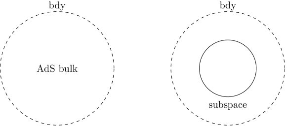
Fig. 1: (Deformed) AdS/CFT. Left: Integrating out fields on the bulk of AdS gives a partition function of a CFT on the boundary(bdy). Right: Integrating out fields on the complement of a subspace gives a partition function of a deformed CFT on this subspace.

P-adic numbers $\mathbb{Q}_{p}$ is introduced by K.Hensel in 1897. One motivation of studying physics over $\mathbb{Q}_{p}$ comes from the possibility that spacetime is non-Archimedean under small scales [7], where expressions of physical laws may be simpler if written in non-Archimedean number fields such as $\mathbb{Q}_{p}$. Another interesting motivation relates to the ”number field invariance principle” [8] which claims that physical laws should be invariant under the change of number fields. Studying on physics over $\mathbb{Q}_{p}$ begins with p-adic strings [9, 10, 7, 11]. Lots of works followed such as those on gravity [12, 13, 14, 15, 16], on AdS/CFT [17, 18, 19, 20, 21] and on spinor [22, 23, 24]. This paper is devoted to some exact results of (deformed) AdS/CFT over $\mathbb{Q}_{p}$. Referring to Fig.2, the Bruhat-Tits tree $\textrm{T}_{p}$ can be regarded as the AdS space over $\mathbb{Q}_{p}$ [17].

0.85

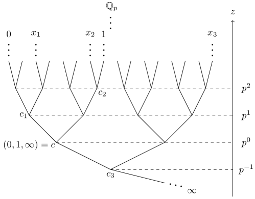
Fig. 2: The Bruhat-tits tree $\textrm{T}_{p}$ with the prime number $p=2$. It is an infinite tree with $p+1$ neighbors for each vertex, and the boundary is $\mathbb{Q}_{p}\cup\{\infty\}$. The p-adic absolute value $|\cdot|_{p}$ can be determined according to the $z$-coordinate. For example, $|x_{1}-x_{2}|_{p}=|z(c)|_{p}=|p^{0}|_{p}=p^{-0}=1$, where $c$ is the lowest vertex on the line connecting $x_{1}$ and $x_{2}$ which is denoted as $\overline{x_{1}x_{2}}$. Similarly we have $|x_{3}|_{p}=|x_{3}-0|_{p}=p^{1}$, $|x_{2}-1|_{p}=p^{-2}$. $c$ is the common vertex of $\overline{0\infty}~{},~{}\overline{01}$ and $\overline{1\infty}$, hence $c=c(0,1,\infty)$.

What are concerned in this paper are two-point functions of (D)CFTs on two special kinds of subspaces of $\textrm{T}_{p}$. Three subspaces are presented in Fig.3, where the left one has been studied in our previous work [21], and the other two are discussed in this paper.

0.85

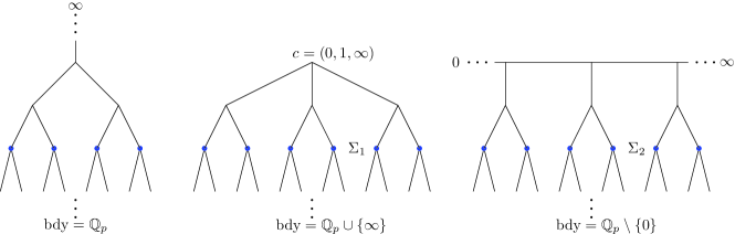
Fig. 3: Three kinds of subspaces(blue vertices) of $\textrm{T}_{p=2}$. They can be taken to the lower boundaries at infinities. The middle one and the right one are denoted as $\Sigma_{1}$ and $\Sigma_{2}$.

The direct motivation of this paper is the comparison between [25] and [21] that the effective action on the lower infinite boundary of the middle one in Fig.3 is considered in the former and effective actions on the finite and lower infinite boundaries of the left one are calculated in the latter. We wonder what do effective actions look like on different subspaces of $\textrm{T}_{p}$ and what’s the limit behaviors when taking these subspaces to infinite boundaries. As shown in the end of section 4, when taken to the lower infinities, $\Sigma_{1}$ and $\Sigma_{2}$ in Fig.3 can be viewed as a circle and a hyperbola over $\mathbb{Q}_{p}$. Please refer to [26, 27] for examples of hyperboloids over $\mathbb{Q}_{p}$, and some results in section 4 can also be found in the latter reference. As for dimensions of variables in this paper, considering that the p-adic absolute value $|\cdot|_{p}$ of the p-adic number $x=p^{k}$ where $k$ is an integer writes

$$|x|_{p}=|p^{k}|_{p}=p^{-k}=x^{-1}~{},$$ (3)

it is convenient to set p-adic numbers and theirs p-adic absolute values dimensionless.

The structure of this paper is as follows: section 2 is the preparation of the action, effective actions on subspaces $\Sigma_{1}$ and $\Sigma_{2}$ are calculated in section 3, two-point functions are given in section 4 and relations between $\Sigma_{1}(\Sigma_{2})$ and a circle(hyperbola) over $\mathbb{Q}_{p}$ are pointed out here too, the last section is the summary and discussion.

2 The Action on $\textrm{T}_{p}$

Consider a free massless scalar field on vertices of $\textrm{T}_{p}$. The action writes

$$S=\frac{1}{2}\sum_{\langle ab\rangle}\frac{(\phi_{a}-\phi_{b})^{2}}{L_{0}^{2}}=\frac{1}{4L_{0}^{2}}\sum_{a}\sum_{b\in\partial a}(\phi_{a}-\phi_{b})^{2}~{}.$$ (4)

$\langle ab\rangle$ means the sum is over all edges of $\textrm{T}_{p}$ whose endpoints are denoted as $a$ and $b$, and $b\in\partial a$ means the sum is over all neighboring vertices of the given vertex $a$. $L_{0}$ is the length of each edge, which is a constant with a dimension of length.

Referring to Fig.4, let’s introduce a $L-$coordinate on $\textrm{T}_{p}$.

0.85

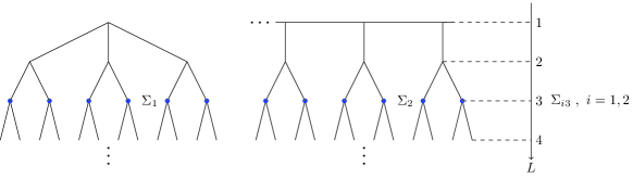
Fig. 4: $L-$coordinate on $\textrm{T}_{p=2}$. Blue vertices identify subspaces $\Sigma_{1}$ and $\Sigma_{2}$ at $L=3$. $\Sigma_{i}~{},~{}i=1,2$ at $L=N$ can be denoted as $\Sigma_{iN}$.

The action can be rewritten as ”field times EOM(equation of motion)” which is

$$S=\frac{1}{2L_{0}^{2}}\sum_{L(a)\leq M}\phi_{a}\Box\phi_{a}+\frac{1}{4L_{0}^{2}}R_{M}(\phi,\phi)+\frac{1}{4L_{0}^{2}}F_{M}(\phi,\phi)~{},$$ (5)

$$R_{M}(f,g):=\sum_{L(a)>M}\sum_{b\in\partial a}(f_{a}-f_{b})(g_{a}-g_{b})~{},~{}F_{M}(f,g):=\sum_{L(a)=M}\sum_{\begin{subarray}{c}b\in\partial a\\ L(b)=M+1\end{subarray}}(f_{a}+f_{b})(g_{b}-g_{a})~{},$$ (6)

$$\Box f_{a}:=\sum_{b\in\partial a}(f_{a}-f_{b}).$$ (7)

$M$ is a positive integer. $f$ and $g$ represent any two fields on $\textrm{T}_{p}$, and ”$:=$” means ”be defined as”. For simplicity, we only consider fields or the field space satisfying $R_{M},F_{M}\to 0$ when $M\to+\infty$, hence the action also writes

$$S=\frac{1}{2L_{0}^{2}}\sum_{a}\phi_{a}\Box\phi_{a}~{}.$$ (8)

The sum is over all vertices of $\textrm{T}_{p}$. Furthermore, in this field space, it can be deduced that

$$\sum_{a}f_{a}\Box g_{a}=\sum_{a}g_{a}\Box f_{a}~{}.$$ (9)

Denote $\Sigma_{1}$ and $\Sigma_{2}$ at $L=N$ as $\Sigma_{iN}$ where $i=1,2$. There is an example for $\Sigma_{i3}$ in Fig.4. Decompose $\phi$ into $\Phi$ which is on-shell on $\textrm{T}_{p}\setminus\Sigma_{iN}$, namely the complement of $\Sigma_{iN}$, and $\phi^{\prime}$ which vanishes on $\Sigma_{iN}$

$$\phi_{a}=\Phi_{a}+\phi^{\prime}_{a}~{},~{}\Box\Phi_{a}|_{a\notin\Sigma_{iN}}=0~{},~{}\phi^{\prime}_{a}|_{a\in\Sigma_{iN}}=0~{}.$$ (10)

With the help of (9), for $N\geq 2$ the action writes

$$S=\frac{1}{2L_{0}^{2}}\sum_{a\in\Sigma_{iN}}\Phi_{a}(\Phi_{a}-\Phi_{a^{-}})+\frac{1}{2L_{0}^{2}}\sum_{a\in\Sigma_{iN}}\Phi_{a}(p\Phi_{a}-\sum_{\begin{subarray}{c}b\in\partial a\\ L(b)>L(a)\end{subarray}}\Phi_{b})+S^{\prime}~{},$$ (11)

$$S^{\prime}=\frac{1}{2L_{0}^{2}}\sum_{a}\phi^{\prime}_{a}\Box\phi^{\prime}_{a}~{},$$ (12)

where $a^{-}$ is the neighboring vertex of $a$ satisfying $L(a^{-})+1=L(a)=N$. We can choose a particular on-shell configuration of $\Phi_{b}$ when $L(b)>L(a)$ such that the second term vanishes, and that leads to

$$S=\frac{1}{2L_{0}^{2}}\sum_{a\in\Sigma_{iN}}\Phi_{a}(\Phi_{a}-\Phi_{a^{-}})+S^{\prime}=S_{N}+S^{\prime}~{}.$$ (13)

If the on-shell $\Phi_{a^{-}}$ can be reconstructed from $\Phi$’s on $\Sigma_{iN}$, $S_{N}$ turns to be an action on $\Sigma_{iN}$. It is found in the end of the next section that $S_{N}$ is the effective action.

3 Field Reconstructions and Effective Actions

There are two equations very useful for the field reconstruction. Consider a special kind of subgraph of $\textrm{T}_{p}$ as shown in Fig.5.

0.85

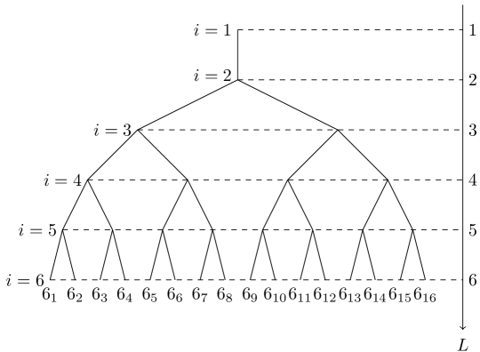
Fig. 5: One subgraph of $\textrm{T}_{p=2}$ with $5$ edges high. The index $i=1,2,\cdots,6$ denotes a vertex at $L=i$, and there are more than one vertex except $i=1,2$. For example, $\phi_{6}$ (the field at $L=6$) can represent any one of $\phi_{6_{1}},\phi_{6_{2}},\phi_{6_{3}},\cdots,\phi_{6_{15}},\phi_{6_{16}}$. Vertices $1$ and $6_{j}~{},~{}j=1,2,\cdots,15,16$ are boundary points of the subgraph.

Image a similar subgraph which is $N-1\geq 2$ edges high, and there are vertices at $L=1,2,\cdots,N-1,N$. Boundary points are located at $L=1,N$. Setting the free massless scalar field inside the boundary on-shell, the first useful equation is the reconstruction of $\phi_{2}$ from $\phi_{1}$ and $\phi_{N}$’s, and it writes

$$\phi_{2}=\frac{p^{N-2}-1}{p^{N-1}-1}\phi_{1}+\frac{p-1}{p^{N-1}-1}\sum_{N\in 2}\phi_{N}~{},~{}N\geq 3~{}.$$ (14)

$\phi_{N}$ represents the field on the lower boundary($L=N$). $N\in 2$ means the sum is over all vertices at $L=N$ those connect to vertex $2$ from below. For example in Fig.5, we have

$$6_{1},6_{2}\in 5~{},~{}6_{1},6_{2},6_{3},6_{4}\in 4~{},~{}6_{1},\cdots,6_{8}\in 3~{},~{}6_{1},\cdots,6_{16}\in 2~{}.$$ (15)

It can be found that $N\in 2$ also means the sum is over all fields on the lower boundary. The equation (14) can be proved by mathematical induction.

The second useful equation is the reconstruction of $\phi_{N-1}$ from $\phi_{1}$ and $\phi_{N}$’s. Replacing $(\phi_{2},\phi_{1},p^{N},N\in 2)$ in (14) with $(\phi_{2},\phi_{1},p^{N},N\in 2),(\phi_{3},\phi_{2},p^{N-1},N\in 3),(\phi_{4},\phi_{3},p^{N-2},N\in 4),\cdots,(\phi_{N-1},\phi_{N-2},p^{3},N\in{N-1})$ gives a set of equations. After eliminating $\phi_{2},\phi_{3},\cdots,\phi_{N-2}$ and introducing a resummation, the reconstruction of $\phi_{N-1}$ writes

$$\begin{aligned} \phi_{N-1}=&\frac{1}{S_{N-1}}\phi_{1}\\ &+\Big{(}\frac{1}{S_{1}S_{2}}+\frac{1}{S_{2}S_{3}}+\cdots+\frac{1}{S_{N-2}S_{N-1}}\Big{)}\sum_{d=2\times 1-1}\phi_{N}\\ &+\Big{(}\frac{1}{S_{2}S_{3}}+\cdots+\frac{1}{S_{N-2}S_{N-1}}\Big{)}\sum_{d=2\times 2-1}\phi_{N}\\ &+\cdots\\ &+\frac{1}{S_{N-2}S_{N-1}}\sum_{d=2\times(N-2)-1}\phi_{N}~{},~{}N\geq 3~{},\end{aligned}$$ (16)

$$S_{k}:=1+p+p^{2}+\cdots+p^{k-1}=\frac{p^{k}-1}{p-1}~{}.$$ (17)

$d$ is the distance(number of edges) between boundary vertices at $L=N$ and the location of $\phi_{N-1}$.

As for the reconstruction of $\Phi_{a^{-}}$ in (13), take the case of $\Sigma_{2}$($\Sigma_{2N}$) in Fig.4 as an example. Please refer to the right in Fig.6 for notations.

0.85

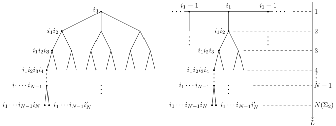
Fig. 6: Notations of vertices for the field reconstruction on $\textrm{T}_{p=2}$. Vertices at $L=1$ are denoted as $i_{1}$, and there is only one vertex $i_{1}$ on the left. On the right there are infinite vertices at $L=1$, which are denoted as $-\infty,\cdots,i_{1}-2,i_{1}-1,i_{1},i_{1}+1,i_{1}+2,\cdots,+\infty$. And vertices at $L=k$ are denoted as $i_{1}i_{2}i_{3}\cdots i_{k}$ where $i_{1}=-\infty,\cdots,+\infty;i_{2}=1,2,\cdots,p-1;i_{3}=1,2,\cdots,p;\cdots;i_{k}=1,2,\cdots,p$. Subspace $\Sigma_{2}$ is located at $L=N$. $i_{1}\cdots i_{N-1}i_{N}$ and $i_{1}\cdots i_{N-1}i_{N}^{\prime}$ are two different vertices belong to the same vertex $i_{1}\cdots i_{N-1}$ when $i_{N}\neq i_{N}^{\prime}$.

According to (16), $\Phi_{i_{1}i_{2}\cdots i_{N-1}}~{},~{}N\geq 3$ can be reconstructed from $\Phi_{i_{1}}$ and $\Phi_{i_{1}^{\prime}i_{2}^{\prime}\cdots i_{N-1}^{\prime}i_{N}^{\prime}}$ as

$$\begin{aligned} \Phi_{i_{1}\cdots i_{N-1}}=&\frac{1}{S_{N-1}}\Phi_{i_{1}}\\ &+\Big{(}\frac{1}{S_{1}S_{2}}+\frac{1}{S_{2}S_{3}}+\cdots+\frac{1}{S_{N-2}S_{N-1}}\Big{)}\sum_{d=2\times 1-1}\Phi_{i_{1}^{\prime}\cdots i_{N}^{\prime}}\\ &+\Big{(}\frac{1}{S_{2}S_{3}}+\cdots+\frac{1}{S_{N-2}S_{N-1}}\Big{)}\sum_{d=2\times 2-1}\Phi_{i_{1}^{\prime}\cdots i_{N}^{\prime}}\\ &+\cdots\\ &+\frac{1}{S_{N-2}S_{N-1}}\sum_{d=2\times(N-2)-1}\Phi_{i_{1}^{\prime}\cdots i_{N}^{\prime}}~{}.\end{aligned}$$ (18)

$d$ is the distance between $i_{1}\cdots i_{N-1}$ and boundary vertex $i_{1}^{\prime}\cdots i_{N}^{\prime}$. Now the remaining question is reconstructing $\Phi_{i_{1}}$ from $\Phi_{i_{1}^{\prime}\cdots i_{N}^{\prime}}$. According to (14), $\Phi_{i_{1}i_{2}}$ can be reconstructed from $\Phi_{i_{1}}$ and $\Phi_{i_{1}^{\prime}\cdots i_{N}^{\prime}}$ as

$$\Phi_{i_{1}i_{2}}=\frac{p^{N-2}-1}{p^{N-1}-1}\Phi_{i_{1}}+\frac{p-1}{p^{N-1}-1}\sum_{i_{1}^{\prime}\cdots i_{N}^{\prime}\in i_{1}i_{2}}\Phi_{i_{1}^{\prime}\cdots i_{N}^{\prime}}~{}.$$ (19)

Summing over $i_{2}$ and using EOM on $i_{1}$ lead to

$$\left\{\begin{aligned} \sum_{i_{2}}\Phi_{i_{1}i_{2}}=&(p-1)\frac{p^{N-2}-1}{p^{N-1}-1}\Phi_{i_{1}}+\frac{p-1}{p^{N-1}-1}\sum_{i_{2}}\sum_{i_{1}^{\prime}\cdots i_{N}^{\prime}\in i_{1}i_{2}}\Phi_{i_{1}^{\prime}\cdots i_{N}^{\prime}}\\ (p+1)\Phi_{i_{1}}=&\Phi_{i_{1}-1}+\Phi_{i_{1}+1}+\sum_{i_{2}}\Phi_{i_{1}i_{2}}\end{aligned}\right.~{}.$$ (20)

Considering that $\sum_{i_{2}}\sum_{i_{1}^{\prime}\cdots i_{N}^{\prime}\in i_{1}i_{2}}=\sum_{i_{1}^{\prime}\cdots i_{N}^{\prime}\in i_{1}}$, eliminating $\sum_{i_{2}}\Phi_{i_{1}i_{2}}$ leads to

$$\Phi_{i_{1}-1}+c\Phi_{i_{1}}+\Phi_{i_{1}+1}=-\frac{p-1}{p^{N-1}-1}\sum_{i_{1}^{\prime}\cdots i_{N}^{\prime}\in i_{1}}\Phi_{i_{1}^{\prime}\cdots i_{N}^{\prime}}~{},~{}c=\frac{p^{N}+p^{N-2}-2}{1-p^{N-1}}~{},$$ (21)

which is also correct for $N=2$. The reconstruction of $\Phi_{i_{1}}$ from $\Phi_{i_{1}^{\prime}\cdots i_{N}^{\prime}}$ requires to find the inverse of the matrix

$$C=\begin{pmatrix}\ddots&&&&&&&&\\ &c&1&&&&&&\\ &1&c&1&&&&&\\ &&1&c&1&&&&\\ &&&1&c&1&&&\\ &&&&1&c&1&&\\ &&&&&1&c&1&\\ &&&&&&1&c&\\ &&&&&&&&\ddots\end{pmatrix}~{}.$$ (22)

And it can be solved by the ansatz

$$C^{-1}=c^{\prime}\begin{pmatrix}\ddots&&&&&&&&\\ &1&e^{-1}&e^{-2}&e^{-3}&e^{-4}&e^{-5}&e^{-6}&\\ &e^{-1}&1&e^{-1}&e^{-2}&e^{-3}&e^{-4}&e^{-5}&\\ &e^{-2}&e^{-1}&1&e^{-1}&e^{-2}&e^{-3}&e^{-4}&\\ &e^{-3}&e^{-2}&e^{-1}&1&e^{-1}&e^{-2}&e^{-3}&\\ &e^{-4}&e^{-3}&e^{-2}&e^{-1}&1&e^{-1}&e^{-2}&\\ &e^{-5}&e^{-4}&e^{-3}&e^{-2}&e^{-1}&1&e^{-1}&\\ &e^{-6}&e^{-5}&e^{-4}&e^{-3}&e^{-2}&e^{-1}&1&\\ &&&&&&&&\ddots\end{pmatrix}~{}.$$ (23)

$CC^{-1}=1$ demands that

$$c^{\prime}=\frac{1}{-\sqrt{c^{2}-4}}~{},~{}e=\frac{-c+\sqrt{c^{2}-4}}{2}~{}.$$ (24)

It can be checked that $c$ in (21) satisfies $c<-2$, and that leads to $e>1$. With the help of $C^{-1}$, $\Phi_{i_{1}}$ can be reconstructed from $\Phi_{i_{1}^{\prime}\cdots i_{N}^{\prime}}$. After a resummation, it writes

$$\Phi_{i_{1}}=\frac{1}{S_{N-1}\sqrt{c^{2}-4}}\Big{(}\sum_{i_{1}^{\prime}\cdots i_{N}^{\prime}\in i_{1}}\Phi_{i_{1}^{\prime}\cdots i_{N}^{\prime}}+\sum_{k=1}^{+\infty}e^{-k}\sum_{d=2\times(N-1)-1+k}\Phi_{i_{1}^{\prime}\cdots i_{N}^{\prime}}\Big{)}~{}.$$ (25)

$d$ is the distance between $i_{1}^{\prime}\cdots i_{N}^{\prime}$ and $i_{1}\cdots i_{N-1}$. Substituting (25) into (18), the reconstruction of $\Phi_{i_{1}\cdots i_{N-1}}$ writes

$$\begin{aligned} \Phi_{i_{1}\cdots i_{N-1}}=&\Big{(}\frac{1}{S_{1}S_{2}}+\frac{1}{S_{2}S_{3}}+\cdots+\frac{1}{S_{N-2}S_{N-1}}+\frac{1}{S_{N-1}^{2}\sqrt{c^{2}-4}}\Big{)}\sum_{d=2\times 1-1}\Phi_{i_{1}^{\prime}\cdots i_{N}^{\prime}}\\ &+\Big{(}\frac{1}{S_{2}S_{3}}+\cdots+\frac{1}{S_{N-2}S_{N-1}}+\frac{1}{S_{N-1}^{2}\sqrt{c^{2}-4}}\Big{)}\sum_{d=2\times 2-1}\Phi_{i_{1}^{\prime}\cdots i_{N}^{\prime}}\\ &+\cdots\\ &+\Big{(}\frac{1}{S_{N-2}S_{N-1}}+\frac{1}{S_{N-1}^{2}\sqrt{c^{2}-4}}\Big{)}\sum_{d=2\times(N-2)-1}\Phi_{i_{1}^{\prime}\cdots i_{N}^{\prime}}\\ &+\frac{1}{S_{N-1}^{2}\sqrt{c^{2}-4}}\sum_{d=2\times(N-1)-1}\Phi_{i_{1}^{\prime}\cdots i_{N}^{\prime}}\\ &+\frac{1}{S_{N-1}^{2}\sqrt{c^{2}-4}}\sum_{k=1}^{+\infty}e^{-k}\sum_{d=2\times(N-1)-1+k}\Phi_{i_{1}^{\prime}\cdots i_{N}^{\prime}}~{},\end{aligned}$$ (26)

which is also correct for $N=2$, hence $N\geq 2$. The field reconstruction in the case of subspace $\Sigma_{1}$ is easier. And the result writes

$$\begin{aligned} \Phi_{i_{1}\cdots i_{N-1}}=&\Big{(}\frac{1}{S_{1}S_{2}}+\frac{1}{S_{2}S_{3}}+\cdots+\frac{1}{S_{N-2}S_{N-1}}+\frac{1}{S_{N-1}S_{2}p^{N-2}}\Big{)}\sum_{d=2\times 1-1}\Phi_{i_{1}^{\prime}\cdots i_{N}^{\prime}}\\ &+\Big{(}\frac{1}{S_{2}S_{3}}+\cdots+\frac{1}{S_{N-2}S_{N-1}}+\frac{1}{S_{N-1}S_{2}p^{N-2}}\Big{)}\sum_{d=2\times 2-1}\Phi_{i_{1}^{\prime}\cdots i_{N}^{\prime}}\\ &+\cdots\\ &+\Big{(}\frac{1}{S_{N-2}S_{N-1}}+\frac{1}{S_{N-1}S_{2}p^{N-2}}\Big{)}\sum_{d=2\times(N-2)-1}\Phi_{i_{1}^{\prime}\cdots i_{N}^{\prime}}\\ &+\frac{1}{S_{N-1}S_{2}p^{N-2}}\sum_{d=2\times(N-1)-1}\Phi_{i_{1}^{\prime}\cdots i_{N}^{\prime}}~{},~{}N\geq 2~{}.\end{aligned}$$ (27)

The vertex notations are the same as those in the case of subspace $\Sigma_{2}$, and they are shown on the left in Fig.6. $d$ still denotes the distance between $i_{1}^{\prime}\cdots i_{N}^{\prime}$ and $i_{1}\cdots i_{N-1}$.

According to the reconstruction of $\Phi_{i_{1}\cdots i_{N-1}}$ in both cases (27) and (26), $\Phi_{a^{-}}$ in (13) can be reconstructed from $\Phi$’s at $\Sigma_{1N}$ and $\Sigma_{2N}$. Together with $S_{N}$ in (13), we have

$$\Sigma_{1N}:~{}\left\{\begin{aligned} \Phi_{a^{-}}=&\sum_{k=1}^{N-1}A_{k}\sum_{\begin{subarray}{c}b\in\Sigma_{1N}\\ d(a^{-},b)=2k-1\end{subarray}}\Phi_{b}=\sum_{b\in\Sigma_{1N}}A_{\frac{1+d(a^{-},b)}{2}}\Phi_{b}\\ A_{n}:=&\frac{1}{S_{n}S_{n+1}}+\frac{1}{S_{n+1}S_{n+2}}+\cdots+\frac{1}{S_{N-2}S_{N-1}}+\frac{1}{S_{N-1}S_{2}p^{N-2}}\\ S_{N}=&\frac{1}{2L_{0}^{2}}\sum_{a\in\Sigma_{1N}}\Phi_{a}(\Phi_{a}-\sum_{b\in\Sigma_{1N}}A_{\frac{1+d(a^{-},b)}{2}}\Phi_{b})=\frac{1}{2L_{0}^{2}}\sum_{a\in\Sigma_{1N}}\Phi_{a}\sum_{b\in\Sigma_{1N}}A_{\frac{1+d(a^{-},b)}{2}}(\Phi_{a}-\Phi_{b})\\ =&\frac{1}{2L_{0}^{2}}\sum_{a\in\Sigma_{1N}}\Phi_{a}\sum_{\begin{subarray}{c}b\in\Sigma_{1N}\\ b\neq a\end{subarray}}A_{\frac{1+d(a^{-},b)}{2}}(\Phi_{a}-\Phi_{b})=\frac{1}{2L_{0}^{2}}\sum_{a\in\Sigma_{1N}}\Phi_{a}\sum_{\begin{subarray}{c}b\in\Sigma_{1N}\\ b\neq a\end{subarray}}A_{\frac{d(a,b)}{2}}(\Phi_{a}-\Phi_{b})\end{aligned}\right.~{},$$ (28)

$$\Sigma_{2N}:~{}\left\{\begin{aligned} \Phi_{a^{-}}=&\sum_{\begin{subarray}{c}b\in\Sigma_{2N}\\ d(a^{-},b)\leq 2(N-1)-1\end{subarray}}B_{\frac{1+d(a^{-},b)}{2}}\Phi_{b}+\sum_{\begin{subarray}{c}b\in\Sigma_{2N}\\ d(a^{-},b)>2(N-1)-1\end{subarray}}C_{1+d(a^{-},b)-2(N-1)}\Phi_{b}\\ B_{n}:=&\frac{1}{S_{n}S_{n+1}}+\frac{1}{S_{n+1}S_{n+2}}+\cdots+\frac{1}{S_{N-2}S_{N-1}}+\frac{1}{S_{N-1}^{2}\sqrt{c^{2}-4}}\\ C_{n}:=&\frac{1}{S_{N-1}^{2}\sqrt{c^{2}-4}}e^{-n}\\ S_{N}=&\frac{1}{2L_{0}^{2}}\sum_{a\in\Sigma_{2N}}\Phi_{a}\Big{(}\sum_{\begin{subarray}{c}b\in\Sigma_{2N}\\ b\neq a\\ d(a,b)\leq 2(N-1)\end{subarray}}B_{\frac{d(a,b)}{2}}(\Phi_{a}-\Phi_{b})+\sum_{\begin{subarray}{c}b\in\Sigma_{2N}\\ d(a,b)>2(N-1)\end{subarray}}C_{d(a,b)-2(N-1)}(\Phi_{a}-\Phi_{b})\Big{)}\end{aligned}\right.~{},$$ (29)

where $d(a^{-},b)$ is the distance between $a^{-}$ and $b$. The following equations have been used:

$$\sum_{b\in\Sigma_{1N}}A_{\frac{1+d(a^{-},b)}{2}}=1~{},$$ (30)

$$\sum_{\begin{subarray}{c}b\in\Sigma_{2N}\\ d(a^{-},b)\leq 2(N-1)-1\end{subarray}}B_{\frac{1+d(a^{-},b)}{2}}+\sum_{\begin{subarray}{c}b\in\Sigma_{2N}\\ d(a^{-},b)>2(N-1)-1\end{subarray}}C_{1+d(a^{-},b)-2(N-1)}=1~{},$$ (31)

$$b\neq a\Rightarrow d(a,b)=d(a^{-},b)+1~{}.$$ (32)

After writing $S_{N}$ as an action on $\Sigma_{iN}$, we can find the effective action by integrating out fields on $\textrm{T}_{p}\setminus\Sigma_{iN}$. Introducing a source $J$ which only lives on $\Sigma_{iN}$, the partition function of $\phi$ writes

$$Z[J]=\frac{\int_{\textrm{T}_{p}}\mathcal{D}\phi e^{-S+\sum_{a\in\Sigma_{iN}}\phi_{a}J_{a}}}{\int_{\textrm{T}_{p}}\mathcal{D}\phi e^{-S}}~{},$$ (33)

where $S$ is the action in (13). In the numerator and denominator, functional integrals on $\textrm{T}_{p}\setminus\Sigma_{iN}$ are the same, hence cancelled. Only those on $\Sigma_{iN}$ are left, and that leads to

$$Z[J]=\frac{\int_{\Sigma_{iN}}\mathcal{D}\Phi e^{-S_{N}+\sum_{a\in\Sigma_{iN}}\Phi_{a}J_{a}}}{\int_{\Sigma_{iN}}\mathcal{D}\Phi e^{-S_{N}}}~{}.$$ (34)

So $S_{N}$ is indeed the effective action on $\Sigma_{iN}$.

4 Two-point Functions of (D)CFTs

According to deformed AdS/CFT

$$\langle e^{\int dxO\phi_{0}}\rangle_{\textrm{DCFT}}=\int_{\textrm{T}_{p}\setminus\Sigma_{iN}}\mathcal{D}\phi e^{-S[\phi]}\Big{|}_{\phi(\Sigma_{iN})=\phi_{0}=\Phi}=e^{-S_{N}}~{},$$ (35)

two point functions of DCFTs at finite boundaries $\Sigma_{iN}$ write

$$\begin{aligned} \Sigma_{1N}:&~{}\langle O_{a}O_{b\neq a}\rangle=\frac{1}{L_{0}^{2}}A_{\frac{d(a,b)}{2}}~{},\\ \Sigma_{2N}:&~{}\langle O_{a}O_{b\neq a}\rangle=\left\{\begin{aligned} \frac{1}{L_{0}^{2}}B_{\frac{d(a,b)}{2}}~{},&~{}d(a,b)\leq 2(N-1)\\ \frac{1}{L_{0}^{2}}C_{d(a,b)-2(N-1)}~{},&~{}d(a,b)>2(N-1)\end{aligned}\right.~{}.\end{aligned}$$ (36)

The case of $N\to+\infty$ is a little complicated, when vertices at $L=N$ approach to boundary points at infinities. Referring to Fig.7,

0.85

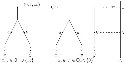
Fig. 7: The limit $N\to+\infty$. The lower infinite boundaries are $\mathbb{Q}_{p}\cup\{\infty\}$ on the left and $\mathbb{Q}_{p}\setminus\{0\}$ on the right.

suppose that $a\to x~{},~{}b(b^{\prime})\to y(y^{\prime})$ when $N\to+\infty$. When fixing boundary points $x,y(y^{\prime})$, the distance between $a$ and $b(b^{\prime})$ tends to infinity, namely $d(a,b),d(a,b^{\prime})\to+\infty$. To found the effective action on the infinite boundary(the lower boundary in Fig.7), we need the limit behaviors of some parameters, and it is found that

$$k\to+\infty:~{}S_{k}=\frac{p^{k}-1}{p-1}\to\frac{p^{k}}{p-1}~{},$$ (37)

$$c=\frac{p^{N}+p^{N-2}-2}{1-p^{N-1}}\to-p-p^{-1}~{},$$ (38)

$$e=\frac{-c+\sqrt{c^{2}-4}}{2}\to p~{},$$ (39)

$$A_{\frac{d(a,b)}{2}},B_{\frac{d(a,b)}{2}},C_{d(a,b)-2(N-1)}\to\frac{p(p-1)}{p+1}p^{-d(a,b)}~{}.$$ (40)

It is unexpected that all three coefficients $A,B,C$ have the same limit behaviors. The effective actions in (28) for $\Sigma_{1N}$ and in (29) for $\Sigma_{2N}$ can be written in a unified form when $N\to+\infty$, which is

$$S_{N}\to\frac{p(p-1)}{2(p+1)L_{0}^{2}}\sum_{a\in\Sigma_{iN}}\Phi_{a}\sum_{\begin{subarray}{c}b\in\Sigma_{iN}\\ b\neq a\end{subarray}}p^{-d(a,b)}(\Phi_{a}-\Phi_{b})~{}.$$ (41)

$\sum$ should be replaced by $\int$ under this limit, and there has to be measure parts which tend to zero. We introduce measures for both cases as shown in Fig.8.

0.85

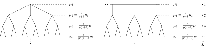
Fig. 8: . Two different measures for vertices on $\textrm{T}_{p=2}$. The measure of a vertex at $L=1$ is denoted as $\mu_{1}$. As for a vertex at $L=n\geq 2$, the measure $\mu_{n}$ is set to $\mu_{n}=\frac{1}{p^{n-2}(p+1)}\mu_{1}$ on the left and $\mu_{n}=\frac{1}{p^{n-2}(p-1)}\mu_{1}$ on the right.

Adding one $\mu_{N}$ behind each $\sum$, effective actions write

$$\Sigma_{1N}:~{}S_{N}\to\frac{p^{2}-1}{2p^{3}\mu_{1}^{2}L_{0}^{2}}\sum_{a\in\Sigma_{1N}}\mu_{N}\Phi_{a}\sum_{\begin{subarray}{c}b\in\Sigma_{1N}\\ b\neq a\end{subarray}}\mu_{N}p^{2N-d(a,b)}(\Phi_{a}-\Phi_{b})~{},$$ (42)

$$\Sigma_{2N}:~{}S_{N}\to\frac{(p-1)^{3}}{2p^{3}(p+1)\mu_{1}^{2}L_{0}^{2}}\sum_{a\in\Sigma_{2N}}\mu_{N}\Phi_{a}\sum_{\begin{subarray}{c}b\in\Sigma_{2N}\\ b\neq a\end{subarray}}\mu_{N}p^{2N-d(a,b)}(\Phi_{a}-\Phi_{b})~{},$$ (43)

where $\sum\mu_{N}\to\int dx$ with a dimension of length. The remaining question is to find the limit of $p^{2N-d}$.

Supposing that $|x|_{p}\leq|y|_{p}$, it can be classified into three cases for $\Sigma_{1N}$: $|x|_{p}\leq|y|_{p}\leq 1$, $|x|_{p}\leq 1<|y|_{p}$ and $1<|x|_{p}\leq|y|_{p}$. Refer to the left and the middle ones in Fig.9 for $|x|_{p}\leq|y|_{p}\leq 1$.

0.85

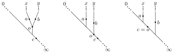
Fig. 9: Different position relations between $x,y$ and $c=(0,1,\infty)$. Left: $|x|_{p}=|y|_{p}\leq 1$. Middle: $|x|_{p}<|y|_{p}\leq 1$. Right: $|x|_{p}\leq 1<|y|_{p}$. The left and middle ones correspond to the case of $|x|_{p}\leq|y|_{p}\leq 1$. The case of $1<|x|_{p}\leq|y|_{p}$ is not shown in this figure. The vertex $o$ is the nearest vertex to $c$ on line $\overline{xy}$.

Comparing with Fig.2 and the left one in Fig.7, it can be found that

$$\left.\begin{aligned} &L(a)=L(b)=N~{},~{}L(c)=1\\ &\frac{d(a,b)}{2}=d(a,o)=d(b,o)=L(b)-L(o)=N-L(o)\\ &|x-y|_{p}=|z(o)|_{p}=|p^{L(o)-1}|_{p}=p^{1-L(o)}=p^{1+\frac{d(a,b)}{2}-N}\end{aligned}\right\}\Rightarrow p^{2N-d(a,b)}=\frac{p^{2}}{|x-y|_{p}^{2}}~{}.$$ (44)

Referring to the right one in Fig.9, for $|x|_{p}\leq 1<|y|_{p}$ it can be found that

$$\frac{d(a,b)}{2}=d(a,c)=N-1\Rightarrow p^{2N-d(a,b)}=p^{2}~{}.$$ (45)

As the case of $1<|x|_{p}\leq|y|_{p}$, applying a transformation on the boundary of $\textrm{T}_{p}$: $x\to x^{\prime}=\frac{1}{x}$ which is an isometric transformation [17] and a rotation around $c=(0,1,\infty)$ of $\textrm{T}_{p}$ which keeps the distance $d(a,b)$ and the $L$-coordinate $N$ in (42) invariant leads to the case of $|y^{\prime}|_{p}\leq|x^{\prime}|_{p}<1$. And that has been solved in (44) already. So we can write

$$p^{2N-d(a,b)}=\frac{p^{2}}{\Big{|}\frac{1}{y}-\frac{1}{x}\Big{|}_{p}^{2}}~{}.$$ (46)

Consider the case of $p\equiv 3\pmod{4}$ when $-1$ has no square root in $\mathbb{Q}_{p}$. The identity $|x^{2}+y^{2}|_{p}=|x^{2},y^{2}|_{s}$ [28] can be used to write (44), (45) and (46) into the same form. Here $|x^{2},y^{2}|_{s}$ gives the maximal one between $|x^{2}|_{p}$ and $|y^{2}|_{p}$. It can be verified that

$$p^{2N-d(a,b)}=p^{2}\frac{|1+x^{2}|_{p}|1+y^{2}|_{p}}{|x-y|_{p}^{2}}~{}.$$ (47)

We set $p\equiv 3\pmod{4}$ here and below.

In the case of $\Sigma_{2N}$, still supposing that $|x|_{p}\leq|y|_{p}$, there are two different position relations between $x,y$ and $\overline{0\infty}$ which are shown in Fig.10.

0.85

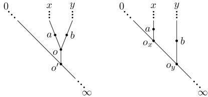
Fig. 10: .Different position relations between $x,y$ and $\overline{0\infty}$. Left: $|x|_{p}=|y|_{p}$. Right: $|x|_{p}<|y|_{p}$.

Referring to Fig.2, the left in Fig.10 and the right in Fig.7, for $|x|_{p}=|y|_{p}$ we have

$$\left.\begin{aligned} &\frac{d(a,b)}{2}=d(a,o)=L(a)-L(o)=N-L(o)\\ &|x|_{p}=|y|_{p}~{},~{}\frac{|x|_{p}}{|x-y|_{p}}=\frac{|z(o^{\prime})|_{p}}{|z(o)|_{p}}=p^{d(o,o^{\prime})}=p^{L(o)-1}\end{aligned}\right\}\Rightarrow p^{2N-d(a,b)}=p^{2}\frac{|x|_{p}^{2}}{|x-y|_{p}^{2}}=p^{2}\frac{|xy|_{p}}{|x-y|_{p}^{2}}~{}.$$ (48)

Referring to the right in Fig.10, for $|x|_{p}<|y|_{p}$ we have

$$\left.\begin{aligned} &d(a,b)=d(a,o_{x})+d(b,o_{y})+d(o_{x},o_{y})=2(N-1)+d(o_{x},o_{y})\\ &\frac{|y|_{p}}{|x|_{p}}=\frac{|z(o_{y})|_{p}}{|z(o_{x})|_{p}}=p^{d(o_{x},o_{y})}~{},~{}|y|_{p}=|x-y|_{p}\end{aligned}\right\}$$ (49)

$$\Rightarrow p^{2N-d(a,b)}=p^{2}\frac{|x|_{p}}{|y|_{p}}=p^{2}\frac{|xy|_{p}}{|y|_{p}^{2}}=p^{2}\frac{|xy|_{p}}{|x-y|_{p}^{2}}~{}.$$ (50)

So in the case of $\Sigma_{2N}$, we can always write

$$p^{2N-d(a,b)}=p^{2}\frac{|xy|_{p}}{|x-y|_{p}^{2}}~{}.$$ (51)

Finally, substituting (47) for $\Sigma_{1N}$ and (51) for $\Sigma_{2N}$ into (42) and (43), effective actions on infinite boundaries ($N\to+\infty$) write

$$\Sigma_{1N}:~{}S_{N}\to\frac{p^{2}-1}{2p\mu_{1}^{2}L_{0}^{2}}\int_{x\in\mathbb{Q}_{p}\cup\{\infty\}}d^{(1)}x\Phi_{x}\int_{\begin{subarray}{c}y\in\mathbb{Q}_{p}\cup\{\infty\}\\ y\neq x\end{subarray}}d^{(1)}y\frac{\Phi_{x}-\Phi_{y}}{|x-y|_{1}^{2}}~{},~{}|x-y|_{1}:=\sqrt{\frac{|x-y|_{p}^{2}}{|1+x^{2}|_{p}|1+y^{2}|_{p}}}~{},$$ (52)

$$\Sigma_{2N}:~{}S_{N}\to\frac{(p-1)^{3}}{2p(p+1)\mu_{1}^{2}L_{0}^{2}}\int_{x\in\mathbb{Q}_{p}\setminus\{0\}}d^{(2)}x\Phi_{x}\int_{\begin{subarray}{c}y\in\mathbb{Q}_{p}\setminus\{0\}\\ y\neq x\end{subarray}}d^{(2)}y\frac{\Phi_{x}-\Phi_{y}}{|x-y|_{2}^{2}}~{},~{}|x-y|_{2}:=\sqrt{\frac{|x-y|_{p}^{2}}{|xy|_{p}}}~{},$$ (53)

where $\Phi_{a}\to\Phi_{x}~{},~{}\Phi_{b}\to\Phi_{y}$ and $\Sigma_{iN}\mu_{N}\to\int d^{(i)}x$ have been used. Two-point functions of CFTs at infinite boundaries write

$$\begin{aligned} \Sigma_{1N}:&~{}\langle O_{x}O_{y\neq x}\rangle=\frac{p^{2}-1}{p\mu_{1}^{2}L_{0}^{2}}\frac{1}{|x-y|_{1}^{2}}~{},\\ \Sigma_{2N}:&~{}\langle O_{x}O_{y\neq x}\rangle=\frac{(p-1)^{3}}{p(p+1)\mu_{1}^{2}L_{0}^{2}}\frac{1}{|x-y|_{2}^{2}}~{}.\end{aligned}$$ (54)

It is interesting that $|x-y|_{1}$ and $|x-y|_{2}$ can be regarded as chordal distances of a circle and a hyperbola. Introducing embedding coordinates for $\Sigma_{1N}$ and $\Sigma_{2N}$ where $N\to+\infty$. In the case of $\Sigma_{1N}$ we write

$$x\to(X_{1},X_{2})~{},~{}y\to(Y_{1},Y_{2}):$$ (55)

$$\left\{\begin{aligned} &x=\frac{X_{1}}{L^{\prime}+X_{2}}\\ &X_{1}=\frac{2x}{1+x^{2}}L^{\prime}~{},~{}X_{2}=\frac{1-x^{2}}{1+x^{2}}L^{\prime}\end{aligned}\right.~{},~{}\left\{\begin{aligned} &y=\frac{Y_{1}}{L^{\prime}+Y_{2}}\\ &Y_{1}=\frac{2y}{1+y^{2}}L^{\prime}~{},~{}Y_{2}=\frac{1-y^{2}}{1+y^{2}}L^{\prime}\end{aligned}\right.~{},$$ (56)

where $L^{\prime}$ is a dimensionless p-adic number. First, it can be found that

$$X_{1}^{2}+X_{2}^{2}=L^{\prime 2}~{},~{}Y_{1}^{2}+Y_{2}^{2}=L^{\prime 2}~{}.$$ (57)

So $(X_{1},X_{2})$ and $(Y_{1},Y_{2})$ can be regarded as two points on the same circle whose radius depends on $L^{\prime}$. Second, it can be verified that

$$|(X_{1}-Y_{1})^{2}+(X_{2}-Y_{2})^{2}|_{p}=|L^{\prime}|_{p}^{2}|x-y|_{1}^{2}~{},$$ (58)

where $|4|_{p}=1$ has been used when $p\equiv 3\pmod{4}$. It means $|x-y|_{1}$ can be regarded as the chordal distance between two points on this circle. Introducing another embedding coordinates for $\Sigma_{2N}$ where $N\to+\infty$

$$x\to(X_{1},X_{2})~{},~{}y\to(Y_{1},Y_{2}):$$ (59)

$$\left\{\begin{aligned} &x=\frac{L^{\prime}}{X_{2}-X_{1}}\\ &X_{1}=\frac{x^{2}-1}{2x}L^{\prime}~{},~{}X_{2}=\frac{x^{2}+1}{2x}L^{\prime}\end{aligned}\right.~{},~{}\left\{\begin{aligned} &y=\frac{L^{\prime}}{Y_{2}-Y_{1}}\\ &Y_{1}=\frac{y^{2}-1}{2y}L^{\prime}~{},~{}Y_{2}=\frac{y^{2}+1}{2y}L^{\prime}\end{aligned}\right.~{}.$$ (60)

First, it can be found that

$$X_{1}^{2}-X_{2}^{2}=-L^{\prime 2}~{},~{}Y_{1}^{2}-Y_{2}^{2}=-L^{\prime 2}~{}.$$ (61)

So $(X_{1},X_{2})$ and $(Y_{1},Y_{2})$ can be regarded as two points on the same hyperbola. Second, it can be verified that

$$|(X_{1}-Y_{1})^{2}-(X_{2}-Y_{2})^{2}|_{p}=|L^{\prime}|^{2}|x-y|_{2}^{2}~{},$$ (62)

which means $|x-y|_{2}$ can be regarded as the chordal distance between two points on this hyperbola.

5 Summary and Discussion

Given a free massless scalar field on $\textrm{T}_{p}$, we calculate effective actions on two kinds of subspaces in Fig.4. At $L=N\geq 2$ for $\Sigma_{1N}$ and $\Sigma_{2N}$, these actions write

$$\Sigma_{1N}:~{}S_{N}=\frac{1}{2L_{0}^{2}}\sum_{a\in\Sigma_{1N}}\Phi_{a}\sum_{\begin{subarray}{c}b\in\Sigma_{1N}\\ b\neq a\end{subarray}}A_{\frac{d(a,b)}{2}}(\Phi_{a}-\Phi_{b})~{},$$ (63)

$$\Sigma_{2N}:~{}S_{N}=\frac{1}{2L_{0}^{2}}\sum_{a\in\Sigma_{2N}}\Phi_{a}\Big{(}\sum_{\begin{subarray}{c}b\in\Sigma_{2N}\\ b\neq a\\ d(a,b)\leq 2(N-1)\end{subarray}}B_{\frac{d(a,b)}{2}}(\Phi_{a}-\Phi_{b})+\sum_{\begin{subarray}{c}b\in\Sigma_{2N}\\ d(a,b)>2(N-1)\end{subarray}}C_{d(a,b)-2(N-1)}(\Phi_{a}-\Phi_{b})\Big{)}~{}.$$ (64)

$d(a,b)$ gives the distance(number of edges) between vertex $a$ and vertex $b$. Coefficients $A,B,C$ write

$$A_{n}=\frac{1}{S_{n}S_{n+1}}+\frac{1}{S_{n+1}S_{n+2}}+\cdots+\frac{1}{S_{N-2}S_{N-1}}+\frac{1}{S_{N-1}S_{2}p^{N-2}}~{},$$ (65)

$$B_{n}=\frac{1}{S_{n}S_{n+1}}+\frac{1}{S_{n+1}S_{n+2}}+\cdots+\frac{1}{S_{N-2}S_{N-1}}+\frac{1}{S_{N-1}^{2}\sqrt{c^{2}-4}}~{},$$ (66)

$$C_{n}=\frac{1}{S_{N-1}^{2}\sqrt{c^{2}-4}}e^{-n}~{},$$ (67)

$$S_{k}=\frac{p^{k}-1}{p-1}~{},~{}c=\frac{p^{N}+p^{N-2}-2}{1-p^{N-1}}~{},~{}e=\frac{-c+\sqrt{c^{2}-4}}{2}~{}.$$ (68)

According to the p-adic version of AdS/CFT, two-point functions of deformed CFTs on $\Sigma_{1N}$ and $\Sigma_{2N}$ write

$$\begin{aligned} \Sigma_{1N}:&~{}\langle O_{a}O_{b\neq a}\rangle=\frac{1}{L_{0}^{2}}A_{\frac{d(a,b)}{2}}~{},\\ \Sigma_{2N}:&~{}\langle O_{a}O_{b\neq a}\rangle=\left\{\begin{aligned} \frac{1}{L_{0}^{2}}B_{\frac{d(a,b)}{2}}~{},&~{}d(a,b)\leq 2(N-1)\\ \frac{1}{L_{0}^{2}}C_{d(a,b)-2(N-1)}~{},&~{}d(a,b)>2(N-1)\end{aligned}\right.~{}.\end{aligned}$$ (69)

When $N\to+\infty$, $\Sigma_{1N}$ and $\Sigma_{2N}$ approach infinite boundaries. The corresponding effective actions and two-point functions of CFTs write

$$\Sigma_{1N}:~{}\left\{\begin{aligned} S_{N}\to&\frac{p^{2}-1}{2p\mu_{1}^{2}L_{0}^{2}}\int_{x\in\mathbb{Q}_{p}\cup\{\infty\}}d^{(1)}x\Phi_{x}\int_{\begin{subarray}{c}y\in\mathbb{Q}_{p}\cup\{\infty\}\\ y\neq x\end{subarray}}d^{(1)}y\frac{\Phi_{x}-\Phi_{y}}{|x-y|_{1}^{2}}\\ \langle O_{x}O_{y\neq x}\rangle=&\frac{p^{2}-1}{p\mu_{1}^{2}L_{0}^{2}}\frac{1}{|x-y|_{1}^{2}}\end{aligned}\right.~{},$$ (70)

$$\Sigma_{2N}:~{}\left\{\begin{aligned} S_{N}\to&\frac{(p-1)^{3}}{2p(p+1)\mu_{1}^{2}L_{0}^{2}}\int_{x\in\mathbb{Q}_{p}\setminus\{0\}}d^{(2)}x\Phi_{x}\int_{\begin{subarray}{c}y\in\mathbb{Q}_{p}\setminus\{0\}\\ y\neq x\end{subarray}}d^{(2)}y\frac{\Phi_{x}-\Phi_{y}}{|x-y|_{2}^{2}}\\ \langle O_{x}O_{y\neq x}\rangle=&\frac{(p-1)^{3}}{p(p+1)\mu_{1}^{2}L_{0}^{2}}\frac{1}{|x-y|_{2}^{2}}\end{aligned}\right.~{}.$$ (71)

$d^{(1)}x$ and $d^{(2)}x$ denote two measures on infinite boundaries which come from $\mu_{N}$ in Fig.8. In the case of $p\equiv 3\pmod{4}$, $|x-y|_{1}$ and $|x-y|_{2}$ can be written using p-adic absolute value $|\cdot|_{p}$ as

$$|x-y|_{1}=\sqrt{\frac{|x-y|_{p}^{2}}{|1+x^{2}|_{p}|1+y^{2}|_{p}}}~{},~{}|x-y|_{2}=\sqrt{\frac{|x-y|_{p}^{2}}{|xy|_{p}}}~{}.$$ (72)

Together with our previous work [21], it can be found that effective actions and two-point functions are very different on three subspaces in Fig.3 but become similar when taken to infinities. This fact comes from the same limit behavior of coefficients $A,B,C$ in (40).

Introducing embedding coordinates (56) and (60), it is found that

$$\left\{\begin{aligned} &x\to(X_{1},X_{2})~{},~{}y\to(Y_{1},Y_{2})\\ &X_{1}^{2}+X_{2}^{2}=L^{\prime 2}~{},~{}Y_{1}^{2}+Y_{2}^{2}=L^{\prime 2}\\ &|x-y|_{1}^{2}=\frac{1}{|L^{\prime}|_{p}^{2}}|(X_{1}-Y_{1})^{2}+(X_{2}-Y_{2})^{2}|_{p}\end{aligned}\right.~{},~{}\left\{\begin{aligned} &x\to(X_{1},X_{2})~{},~{}y\to(Y_{1},Y_{2})\\ &X_{1}^{2}-X_{2}^{2}=-L^{\prime 2}~{},~{}Y_{1}^{2}-Y_{2}^{2}=-L^{\prime 2}\\ &|x-y|_{2}^{2}=\frac{1}{|L^{\prime}|_{p}^{2}}|(X_{1}-Y_{1})^{2}-(X_{2}-Y_{2})^{2}|_{p}\end{aligned}\right.~{}.$$ (73)

So the infinite boundary $\Sigma_{1N}$ when $N\to+\infty~{}$ on the left in Fig.4 can be regarded as a circle over p-adic numbers, and $|x-y|_{1}$ as the chordal distance between $x$ and $y$ on it. Similarly, $\Sigma_{2N}$ when $N\to+\infty~{}$ on the right in Fig.4 can be regarded as a hyperbola, and $|x-y|_{2}$ as its chordal distance.

Several problems are still unsolved, for example, (i)what’s the results on other subspaces besides those in Fig.3 or in the case of $p\equiv 1\pmod{4}$? (ii)is the limit behavior of coefficients $A,B,C$ in (40) universal? (iii)what’s the meaning of our results to CFTs over p-adic numbers?