Retrospective Cost-based Extremum Seeking Control with Vanishing Perturbation for Online Output Minimization

Abstract

Extremum seeking control (ESC) constitutes a powerful technique for online optimization with theoretical guarantees for convergence to the neighborhood of the optimizer under well-understood conditions. However, ESC requires a nonconstant perturbation signal to provide persistent excitation to the target system to yield convergent results, which usually results in steady state oscillations. While certain techniques have been proposed to eliminate perturbations once the neighborhood of the minimizer is reached, system modifications and environmental perturbations can suddenly change the minimizer and nonconstant perturbations would once more be required to convergence to the new minimizer. Hence, this paper develops a retrospective cost-based ESC (RC/ESC) technique for online output minimization with a vanishing perturbation, that is, a perturbation that becomes zero as time increases independently from the state of the controller or the controlled system. The performance of the proposed algorithm is illustrated via numerical examples.

I Introduction

Extremum seeking control (ESC) is a powerful adaptive control technique that leverages persistent system excitation to search for extrema in order to either minimize or maximize a used-defined metric [1]. The stability and convergence properties of ESC and their conditions have been thoroughly studied and are well understood [2, 3, 4]. ESC has been applied in a wide arrange of fields, including robotics [5, 6, 7, 8, 9, 10, 11, 12] and energy management [13, 14, 15, 16, 17, 18, 19].

A feature of ESC is a persistent perturbation signal, which enables gradient estimation algorithms to yield a search direction that points towards local extrema, thus enabling convergence. However, the implementation of this perturbation signal results in steady state oscillations, which may be prohibitive in physical testing. Modifications to the ESC algorithm have been proposed to address this issue, which include modifying the perturbation signal to vanish depending on controller and system values and implementing dynamics that suppress the perturbation signal once a neighborhood of the minimizer has been reached [20, 21, 22, 23, 24].

The contribution of this paper is thus an ESC algorithm for online output minimization with a vanishing perturbation, that is, a perturbation that becomes zero as time increases independently from the state of the controller or the controlled system. Hence, the perturbation is independent from the rest of the system and no extra dynamics are required to suppress the perturbation. In particular, we consider retrospective cost adaptive control (RCAC), which re-optimizes the coefficients of the feedback controller at each step [25]. A similar retrospective cost algorithm was proposed in [26, 27], in which a fixed target model was used to issue a search direction in the input space for optimization. In this work, a Kalman Filter (KF) is used to estimate the gradient of the system output which is encoded into the target model to provide a time-varying search direction to RCAC. Hence, the combination of the KF, the target model construction procedure, and RCAC yields retrospective cost based ESC (RC/ESC). A preliminary version of this algorithm was considered in [28], in which gradient estimation was performed by using a simple high-pass filter.

The contents of the paper are as follows. Section II provides a statement of the control problem, which involves continuous-time dynamics under sampled-data feedback control. Section III provides a review of continuous-time ESC. Section IV introduces RC/ESC, in which a KF estimates the gradient of the system output and provides a target model to RCAC. Section V presents numerical examples that illustrate the performance of RC/ESC, including examples with static maps and a example with a dynamic system. Finally, VI presents conclusions.

Notation: ${\bf q}\in{\mathbb{C}}$ denotes the forward-shift operator. $x_{(i)}$ denotes the $i$th component of $x\in{\mathbb{R}}^{n}.$

II Problem Statement

We consider continuous-time dynamics under sampled-data control using discrete-time adaptive controllers to reflect the practical implementation of digital controllers for physical systems. In particular, we consider the control architecture shown in Figure 1, where ${\mathcal{M}}$ is the target continuous-time system, $t\geq 0$, $u(t)\in{\mathbb{R}}^{m}$ is the control, and $J(t)\in{\mathbb{R}}^{p}$ is the output of ${\mathcal{M}},$ whose components are all non-negative.

The output $J(t)$ is sampled to generate the measurement $J_{k}\in{\mathbb{R}}^{p},$ which, for all $k\geq 0,$ is given by

$$J_{k}\stackrel{{\scriptstyle\triangle}}{{=}}J(kT_{\rm s}),$$ (1)

where $T_{\rm s}>0$ is the sample time. The adaptive controller, which is updated at each step $k,$ is denoted by ${\mathcal{G}}_{{\rm c},k}$. The input to ${\mathcal{G}}_{{\rm c},k}$ is $J_{k}$, and its output at each step $k$ is the discrete-time control $u_{k}\in{\mathbb{R}}^{m}.$ The continuous-time control signal $u(t)$ applied to the structure is generated by applying a zero-order-hold operation to $u_{k},$ that is, for all $k\geq 0,$ and, for all $t\in[kT_{\rm s},(k+1)T_{\rm s}),$

$$u(t)=u_{k}.$$ (2)

The objective of the adaptive controller is to yield an input signal that minimizes the output of the continuous-time system, that is, yield $u(t)$ such that $\lim_{t\to\infty}J(t)=0.$

Figure 1: Sampled-data implementation of adaptive controller for control of the continuous-time system ${\mathcal{M}}.$ All sample-and-hold operations are synchronous. The adaptive controller uses $J_{k}$ as an input and generates the discrete-time control $u_{k}$ at each step $k$. Note that all components of $J_{k}$ are nonnegative. The resulting continuous-time control $u(t)$ is generated by applying a zero-order-hold operation to $u_{k}$. The objective of the controller is yield an input signal that minimizes the output of the continuous-time system, that is, yield $u(t)$ such that $\lim_{t\to\infty}J(t)=0.$

III Overview of Extremum Seeking Control

III-A General Scheme

Consider the system ${\mathcal{M}}$ shown in first order extremum seeking scheme displayed in figure 2 to be

$$\dot{x} =f(x,u),$$ (3)

$$J(t) ={\mathcal{Q}}(x),$$ (4)

where $f:\mathbb{R}^{n}\times\mathbb{R}^{m}\to\mathbb{R}^{n}$ and ${\mathcal{Q}}(x):\mathbb{R}^{n}\to\mathbb{R}^{p}$ are smooth enough, $x\in\mathbb{R}^{n}$ is the measured vector state, $u\in\mathbb{R}^{m}$ is the input vector and $J(t)\in\mathbb{R}^{p}$ is the output of the cost function ${\mathcal{Q}}(x)$. Suppose that there exists $x^{*}$ such that $J^{*}={\mathcal{Q}}(x^{*})$ is the extremum of the map ${\mathcal{Q}}(.)$. Assume that both $x^{*}$ and ${\mathcal{Q}}(.)$ are unknown. Thus, the main goal of extremum seeking control is to drive the states of the closed loop to $x^{*}$ without knowledge of $x^{*}$ or ${\mathcal{Q}}(.)$

Figure 2: Continuous-time extremum seeking control (ESC) of the continuous-time system ${\mathcal{M}}.$ ESC uses $J$ as an input and generates the control $u_{k}$ at each step $k$. Note that all components of $J$ are nonnegative. The objective of the controller is yield an input signal that minimizes the output of the continuous-time system, that is, yield $u(t)$ such that $\lim_{t\to\infty}J(t)=0.$

III-B SISO case

Consider the case when $J(x)\in\mathbb{R}$, and $u\in\mathbb{R}$ are scalar. Next, consider the dither signal

$$d(t)=a~{}\sin(\omega_{1}~{}t),$$ (5)

where $a$ is the amplitude of the dither signal, and $\omega_{1}$ is the dither frequency. Also, note that the gradient estimator used in this work is based on the averaging technique as proved in [29] such that

$$\tilde{J}_{u}(t) =\dfrac{2}{a}~{}J(t)\sin(\omega_{1}~{}t).$$ (6)

Finally, $\delta u(t)$, computed as the output of ${\mathcal{I}}(t)$ shown in figure 2, is obtained from the gradient descent scheme given by

$$\delta u(t) =K_{\text{esc}}~{}\int_{0}^{t}\tilde{J}_{u}~{}dt.$$ (7)

In this scheme, $a,\omega_{1}$ and $K_{\text{esc}}$ are the tuning parameters.

III-C MISO case

Now, consider the case when $J(x)\in\mathbb{R}$, and $u\in\mathbb{R}^{m}$. Define the vector of dither signals ${\mathcal{D}}(t)\stackrel{{\scriptstyle\triangle}}{{=}}\begin{bmatrix}d_{1}(t)&d_{2}(t)&\cdots&d_{m}(t)\end{bmatrix}^{\rm T}$ given by

$${\mathcal{D}}(t) =a\begin{bmatrix}\sin(\omega_{1}~{}t)\\ \sin(\omega_{2}~{}t)\\ \vdots\\ \sin(\omega_{m}~{}t)\end{bmatrix},$$ (8)

where each $\omega_{1},\omega_{2},\cdots,\omega_{m}$ must be different. Note that although different amplitudes can be chosen for each dither signal, in the present work the same amplitude has been used for all, as shown in (8). Define $\tilde{{\mathcal{J}}}_{u}\stackrel{{\scriptstyle\triangle}}{{=}}\begin{bmatrix}\tilde{J}_{u_{1}}&\tilde{J}_{u_{2}}&\cdots&\tilde{J}_{u_{m}}\end{bmatrix}^{\rm T}$. Then, the gradient estimator based on the work done by [30] is given by

$$\tilde{{\mathcal{J}}}_{u} =\dfrac{2}{a}~{}J(t)\begin{bmatrix}\sin(\omega_{1}~{}t)\\ \sin(\omega_{2}~{}t)\\ \vdots\\ \sin(\omega_{m}~{}t)\end{bmatrix}.$$ (9)

Finally, Define $\Delta u(t)\stackrel{{\scriptstyle\triangle}}{{=}}\begin{bmatrix}\delta u_{1}(t)&\delta u_{2}(t)&\cdots&\delta u_{m}(t)\end{bmatrix}^{\rm T}$ given by the expression

$$\Delta u(t) =K_{\text{esc}}\int_{0}^{t}\tilde{{\mathcal{J}}}_{u}~{}dt.$$ (10)

Note that although different $K_{\text{esc}}$ can be chosen for each component of $\tilde{{\mathcal{J}}}_{u}$, in the proposed scheme only one is considered, as shown in (10). Thus, $a$, $K_{\text{esc}}$ and $\begin{bmatrix}\omega_{1}&\omega_{2}&\cdots&\omega_{m}\end{bmatrix}$ are the tuning parameters.

IV Overview of Retrospective Cost based Extremum Seeking Control

An overview of the RC/ESC algorithm is presented in this section. Subsection IV-A presents a brief review of RCAC. Subsection IV-C describes an online gradient estimator based on the KF. Subsection IV-D expands RCAC presented in Subsection IV-A to include gradient estimates obtained via the technique presented in Subsection IV-C, resulting in RC/ESC.

IV-A Review of Retrospective Cost Adaptive Control

RCAC is described in detail in [25]. In this subsection we summarize the main elements of this method. Consider the strictly proper, discrete-time, input-output controller

$$\delta u_{k}=\sum_{i=1}^{l_{\rm c}}P_{i,k}u_{k-i}+\sum_{i=1}^{l_{\rm c}}Q_{i,k}z_{k-i},$$ (11)

where $k\geq 0$ is the time step, $\delta u_{k}\in{\mathbb{R}}^{m}$ is the RCAC controller output, $u_{k}\in{\mathbb{R}}^{m}$ is the RC/ESC output and thus the control input, $z_{k}\in{\mathbb{R}}^{p}$ is the measured performance variable, $l_{\rm c}$ is the controller-window length, and, for all $i\in\{1,\ldots,l_{\rm c}\},$ $P_{i,k}\in{\mathbb{R}}^{m\times m}$ and $Q_{i,k}\in{\mathbb{R}}^{m\times p}$ are the controller coefficient matrices. In particular, $u_{k}$ results from adding a perturbation signal to $\delta u_{k},$ as shown in Subsection IV-D. The controller shown in (11) can be written as

$$\delta u_{k}=\phi_{k}\theta_{k},$$ (12)

where

$$\phi_{k} \stackrel{{\scriptstyle\triangle}}{{=}}\footnotesize\left[\begin{array}[]{cccccc}u_{k-1}^{\mathsf{T}}&\cdots&u_{k-l_{\rm c}}^{\mathsf{T}}&z_{k-1}^{\mathsf{T}}&\cdots&z_{k-l_{\rm c}}^{\mathsf{T}}\end{array}\right]\otimes I_{m}\in\mathbb{R}^{m\times l_{\theta}},$$ (14)

$$\theta_{k} \stackrel{{\scriptstyle\triangle}}{{=}}{\rm vec}\left[\begin{array}[]{cccccc}P_{1,k}&\cdots&P_{l_{\rm c},k}&Q_{1,k}&\cdots&Q_{l_{\rm c},k}\end{array}\right]\in{\mathbb{R}}^{l_{\theta}},$$ (16)

$l_{\theta}\stackrel{{\scriptstyle\triangle}}{{=}}l_{\rm c}m(m+p),$ $\theta_{k}$ is the vector of controller coefficients, which are updated at each time step $k$, and $\otimes$ is the Kroenecker product.

Next, define the retrospective cost variable

$$\hat{z}_{k}(\hat{\theta})\stackrel{{\scriptstyle\triangle}}{{=}}z_{k}-G_{\rm f}(\textbf{q})(\delta u_{k}-\phi_{k}\hat{\theta}),$$ (17)

where $\hat{z}_{k}$ is the retrospective-cost variable, $G_{{\rm f}}$ is an $p\times m$ asymptotically stable, strictly proper transfer function, q is the forward-shift operator, and $\hat{\theta}\in{\mathbb{R}}^{l_{\theta}}$ is the controller coefficient vector determined by optimization below. The rationale underlying (17) is to replace the applied past control inputs with the re-optimized control input $\phi_{k}\hat{\theta},$ as mentioned in [25] and [31].

In the present work, $G_{{\rm f}}$ is chosen to be a finite-impulse-response transfer function of window length $l_{\rm f}$ of the form

$$G_{{\rm f}}({\bf q})\stackrel{{\scriptstyle\triangle}}{{=}}\sum_{i=1}^{l_{\rm f}}N_{i,k}\textbf{q}^{-i},$$ (18)

where $N_{1,k},\ldots,N_{l_{\rm f},k}\in{\mathbb{R}}^{p\times m}.$ We can thus rewrite (17) as

$$\hat{z}_{k}(\hat{\theta})=z_{k}-N_{k}(U_{k}-{\Phi}_{k}\hat{\theta}),$$ (19)

where

$${\Phi}_{k}\stackrel{{\scriptstyle\triangle}}{{=}}\footnotesize\left[\begin{array}[]{c}\phi_{k-1}\\ \vdots\\ \phi_{k-l_{\rm f}}\\ \end{array}\right]\in{\mathbb{R}}^{l_{\rm f}m\times l_{\theta}},\ U_{k}\stackrel{{\scriptstyle\triangle}}{{=}}\footnotesize\left[\begin{array}[]{c}u_{k-1}\\ \vdots\\ u_{k-l_{\rm f}}\\ \end{array}\right]\in{\mathbb{R}}^{l_{\rm f}m},$$ (26)

$$N_{k}\stackrel{{\scriptstyle\triangle}}{{=}}\footnotesize\left[\ N_{1,k}\ \cdots\ N_{l_{\rm f},k}\ \right]\in{\mathbb{R}}^{p\times l_{\rm f}m}.$$ (27)

In most applications, $N_{k}$ is constant and is determined by features of the system being controlled, as mentioned in [25]. Other applications may require $N_{k}$ to be constructed and updated online using data, as mentioned in [31]. For the present work, the algorithm used to determine $N_{k}$ at each step $k$ is given in the next section.

Using (17), we define the cumulative cost function

$$J_{{\rm R},k}(\hat{\theta})\stackrel{{\scriptstyle\triangle}}{{=}}\sum\limits_{i=0}^{k}[\hat{z}_{i}^{\rm T}(\hat{\theta})\hat{z}_{i}(\hat{\theta})+(\phi_{i}\hat{\theta})^{\rm T}R_{\rm u}\phi_{i}\hat{\theta}]+(\hat{\theta}-\theta_{0})^{\rm T}P_{0}^{-1}(\hat{\theta}-\theta_{0}),$$ (28)

where $P_{0}\in{\mathbb{R}}^{l_{\theta}\times l_{\theta}}$ is positive definite and $R_{\rm u}\in{\mathbb{R}}^{m\times m}$ is positive semidefinite. The following result uses recursive least squares (RLS), as mentioned in [32] and [33], to minimize (28), where, at each step $k,$ the minimizer of (28) provides the update $\theta_{k+1}$ of the controller coefficient vector $\theta_{k}$.

Proposition. Let $P_{0}$ be positive definite, and $R_{\rm u}$ be positive semidefinite. Then, for all $k\geq 0$, unique global minimizer $\theta_{k}$ of (28) is given by

$$P_{k}= \ P_{k-1}-P_{k-1}\left[\begin{array}[]{c}N_{k-1}{\Phi}_{k-1}\\ \phi_{k-1}\end{array}\right]^{\mathsf{T}}\Gamma_{k-1}\left[\begin{array}[]{c}N_{k-1}{\Phi}_{k-1}\\ \phi_{k-1}\end{array}\right]P_{k-1},$$ (33)

$$\theta_{k}= \ \theta_{k-1}$$

$$-P_{k}\left[\begin{array}[]{c}N_{k-1}{\Phi}_{k-1}\\ \phi_{k-1}\end{array}\right]^{\mathsf{T}}\bar{R}\left[\begin{array}[]{cc}z_{k-1}-N_{k-1}(U_{k-1}-{\Phi}_{k-1}\theta_{k-1})\\ \phi_{k-1}\theta_{k-1}\end{array}\right],$$ (38)

where

$$\Gamma_{k-1}\stackrel{{\scriptstyle\triangle}}{{=}} \ \bar{R}-\bar{R}\left[\begin{array}[]{c}N_{k-1}{\Phi}_{k-1}\\ \phi_{k-1}\end{array}\right]\Xi_{k}^{-1}\left[\begin{array}[]{c}N_{k-1}{\Phi}_{k-1}\\ \phi_{k-1}\end{array}\right]^{\mathsf{T}}\bar{R}$$ (43)

$$\in{\mathbb{R}}^{(p+m)\times(p+m)},$$ (44)

$$\Xi_{k}\stackrel{{\scriptstyle\triangle}}{{=}} \ P_{k-1}^{-1}+\left[\begin{array}[]{c}N_{k-1}{\Phi}_{k-1}\\ \phi_{k-1}\end{array}\right]^{\mathsf{T}}\bar{R}\left[\begin{array}[]{c}N_{k-1}{\Phi}_{k-1}\\ \phi_{k-1}\end{array}\right]\in{\mathbb{R}}^{l_{\theta}\times l_{\theta}},$$ (49)

$$\bar{R}\stackrel{{\scriptstyle\triangle}}{{=}} \ {\rm diag}(I_{p},R_{\rm u})\in{\mathbb{R}}^{(p+m)\times(p+m)}.$$ (50)

For all of the numerical simulations and physical experiments in this work, $\theta_{k}$ is initialized as $\theta_{0}=0_{l_{\theta}\times 1}$ to reflect the absence of additional prior modeling information. The matrices $P_{0}$ and $R_{\rm u}$ have the form $P_{0}=p_{0}I_{l_{\theta}}$ and $R_{\rm u}=r_{\rm u}I_{m},$ where the positive scalar $p_{0}$ and nonnegative scalar $r_{\rm u}$ determine the rate of adaptation.

IV-B RCAC-based PID

In the case where $m=p=1,$ let $\delta u_{k}$ be given by

$$\delta u_{k}=\kappa_{{\rm p},k}z_{k-1}+\kappa_{{\rm i},k}\zeta_{k-1}+\kappa_{{\rm d},k}(z_{k-1}-z_{k-2}),$$ (51)

where $\kappa_{{\rm p},k}$, $\kappa_{{\rm i},k}$, and $\kappa_{{\rm d},k}$ are time-varying PID gains and $\zeta_{k}$ is given by the integrator

$$\zeta_{k}\stackrel{{\scriptstyle\triangle}}{{=}}\sum_{j=0}^{k}z_{j}.$$ (52)

The control (51) can be expressed as

$$\delta u_{k}=\phi_{k}\theta_{k},$$ (53)

where

$$\phi_{k}\stackrel{{\scriptstyle\triangle}}{{=}} \begin{bmatrix}z_{k-1}&\zeta_{k-1}&z_{k-1}-z_{k-2}\end{bmatrix}\in\mathbb{R}^{1\times 3},$$ (54)

$$\theta_{k}\stackrel{{\scriptstyle\triangle}}{{=}} \begin{bmatrix}\kappa_{{\rm p},k}&\kappa_{{\rm i},k}&\kappa_{{\rm d},k}\end{bmatrix}^{\mathsf{T}}\in\mathbb{R}^{3}.$$ (55)

Note that the regressor $\phi_{k}$ is constructed from the past values of $z_{k}$ and $\zeta_{k},$ and the controller coefficient vector $\theta_{k}$ contains the time-dependent proportional, integral, and derivative gains $\kappa_{{\rm p},k},$ $\kappa_{{\rm i},k},$ and $\kappa_{{\rm d},k}$. Furthermore, note that the adaptive digital PID control can be specialized to adaptive digital PI, PD, ID, P, I, and D control by omitting the corresponding components of $\phi_{k}$ and $\theta_{k}.$ Then, RCAC-based PID (RCAC/PID) can be implemented by replacing (14) and (16) with (54) and (55), respectively.

IV-C Online gradient estimator using a Kalman Filter

For all $k\geq 0,$ let $J_{k}\stackrel{{\scriptstyle\triangle}}{{=}}[J_{1,k}\ \ \cdots\ \ J_{l_{J},k}]^{\mathsf{T}}\in{\mathbb{R}}^{l_{J}}$ be a cost function vector computed from system measurements, where, for all $i\in\{1,\ldots,l_{J}\},$ $J_{i,k}\geq 0$ is the $i$th component of $J_{k},$ let $u_{k}$ be the control input, and let $\nabla J_{k}\stackrel{{\scriptstyle\triangle}}{{=}}[\nabla J_{1,k}\ \ \cdots\ \ \nabla J_{l_{J},k}]^{\mathsf{T}}\in{\mathbb{R}}^{l_{J}\times m}$ be the gradient of $J_{k}$ over $u_{k},$ where, for all $i\in\{1,\ldots,l_{J}\},$ the transpose of $\nabla J_{i,k}\in{\mathbb{R}}^{m}$ corresponds to the $i$th row of $\nabla J_{k}.$

Next, let $i\in\{1,\ldots,l_{J}\}.$ Consider the measurement model for $J_{i,k}$

$$J_{i,k}=J_{{\rm b},i}+\nabla J_{i,k}^{\mathsf{T}}u_{k},$$ (56)

where $J_{{\rm b},i}\in{\mathbb{R}}$ is a bias variable. Note that (56) is an extension of (17) from [34]. Furthermore, let $\nabla\hat{J}_{i,k}\in{\mathbb{R}}^{m}$ be an estimate of $\nabla J_{i,k},$ let $\hat{J}_{{\rm b},i}\in{\mathbb{R}}$ be an estimate of $J_{{\rm b},i},$ let $\hat{x}_{i,k}\stackrel{{\scriptstyle\triangle}}{{=}}\begin{bmatrix}\nabla\hat{J}_{i,k}^{\mathsf{T}}&\hat{J}_{{\rm b},i}\end{bmatrix}^{\mathsf{T}}\in{\mathbb{R}}^{m+1}$ be an estimate of $x_{i,k}\stackrel{{\scriptstyle\triangle}}{{=}}\begin{bmatrix}\nabla J_{i,k}^{\mathsf{T}}&J_{{\rm b},i}\end{bmatrix}^{\mathsf{T}},$ and let $P_{i,k}\in{\mathbb{R}}^{(m+1)\times(m+1)}$ be the covariance of the estimate $\hat{x}_{i,k}$ of $x_{i,k}.$ Then, as indicated by (56) and Section 3.1 of [34], the estimate $\nabla\hat{J}_{i,k}$ can be obtained using a KF with state and measurement equations given by

$$x_{i,k+1} =x_{i,k}+w_{i,k},$$ (57)

$$y_{i,k}\stackrel{{\scriptstyle\triangle}}{{=}}\begin{bmatrix}J_{i,k}\\ J_{i,k-k_{1}}\\ \vdots\\ J_{i,k-k_{m}}\end{bmatrix} =\begin{bmatrix}u_{k-1}^{\mathsf{T}}&1\\ u_{k-1-k_{1}}^{\mathsf{T}}&1\\ \vdots&\vdots\\ u_{k-1-k_{m}}^{\mathsf{T}}&1\end{bmatrix}x_{i,k}+v_{i,k},$$ (58)

where $y_{i,k}\in{\mathbb{R}}^{m+1}$ is the measurement vector and $w_{i,k},v_{i,k}\in{\mathbb{R}}^{m+1}$ are Gaussian random variables. Hence, it follows from (57), (58) that the estimate $\nabla\hat{J}_{i,k}$ is given by the recursive update of the KF, whose prediction and update equations are given, for $i\in\{1,\ldots,l_{J}\},$ by

$$\hat{x}_{i,k} =\hat{x}_{i,k-1}+K_{i,k-1}\left(G_{i,k-1}-H_{k-1}\hat{x}_{i,k-1}\right),$$ (59)

$$P_{i,k} =(I_{m+1}-K_{i,k-1}H_{k-1})(P_{i,k-1}+Q_{i}),$$ (60)

$$\nabla\hat{J}_{i,k} =\left[I_{m}\ \ 0_{m\times 1}\right]\hat{x}_{i,k},$$ (61)

where

$$G_{i,k-1}\stackrel{{\scriptstyle\triangle}}{{=}}\begin{bmatrix}J_{i,k-1}\\ J_{i,k-1-k_{1}}\\ \vdots\\ J_{i,k-1-k_{m}}\end{bmatrix}\in{\mathbb{R}}^{m+1},\ H_{k-1}\stackrel{{\scriptstyle\triangle}}{{=}} \ \begin{bmatrix}u_{k-1}^{\mathsf{T}}&1\\ u_{k-1-k_{1}}^{\mathsf{T}}&1\\ \vdots&\vdots\\ u_{k-1-k_{m}}^{\mathsf{T}}&1\end{bmatrix}$$

$$\ \in{\mathbb{R}}^{(m+1)\times(m+1)},$$

$$K_{i,k-1}\stackrel{{\scriptstyle\triangle}}{{=}} \ [(P_{i,k-1}+Q_{i})H_{k-1}^{\mathsf{T}}][H_{k-1}(P_{i,k-1}+Q_{i})H_{k-1}^{\mathsf{T}}+R_{i}]^{-1}$$

$$\ \in{\mathbb{R}}^{(m+1)\times(m+1)},$$

$Q_{i},R_{i}\in{\mathbb{R}}^{(m+1)\times(m+1)}$ are the constant weighting matrices, and $0<k_{1}<\dots<k_{m}$ are indices. The matrices $Q_{i}$ and $R_{i}$ determine the rate of estimation, and $k_{1},\ldots,k_{m}$ are chosen to enhance the accuracy of the estimate $\hat{x}_{i,k}.$ Finally, the estimate $\nabla\hat{J}_{k}$ is given by

$$\nabla\hat{J}_{k}\stackrel{{\scriptstyle\triangle}}{{=}}\left[\nabla\hat{J}_{1,k}\ \ \cdots\ \ \nabla\hat{J}_{l_{J},k}\right]^{\mathsf{T}}\in{\mathbb{R}}^{l_{J}\times m}.$$ (62)

For all of the numerical simulations in the present work, $\hat{x}_{i,k}$ is initialized as $\hat{x}_{i,0}=0_{m\times 1}.$ The matrices $P_{i,0},$ $Q_{i},$ and $R_{i}$ have the form $P_{i,0}=p_{i,0}I_{m+1},$ $Q_{i}=q_{i}I_{m+1},$ and $R_{i}=r_{i}I_{m+1},$ where the positive scalars $p_{i,0},$ $q_{i},$ and $r_{i}$ determine the rate of estimation.

IV-D Retrospective Cost based Extremum Seeking Control

As shown in Figure 3, RC/ESC includes RCAC described in Subsection IV-A, the KF gradient estimator described in Subsection IV-C, a normalization function, and a gradient conversion function. For RC/ESC, $l_{J}=p$ and $l_{\rm f}=m.$ RC/ESC operates on the cost-function vector $J_{k}\in{\mathbb{R}}^{p}$ and $u_{k-1}\in{\mathbb{R}}^{m}$ to produce the RC/ESC output vector $u_{k}\in{\mathbb{R}}^{m}.$ As mentioned in subsection IV-C, for all $i\in\{1,\ldots,p\},$ $J_{i,k}>0.$ The objective of RC/ESC is to minimize the components of $J_{k}$ by modulating $u_{k},$ that is,

$$\min_{(u_{n})_{n=0}^{\infty}}\ \ \limsup_{k\to\infty}\sum_{i=1}^{p}J_{i,k}.$$ (63)

The performance variable $z_{k}$ used by RCAC is obtained by normalizing $J_{k}$ using

$$z_{k}\stackrel{{\scriptstyle\triangle}}{{=}}[I_{p}+\nu\ {\rm diag}\left(J_{k}\right)]^{-1}J_{k},$$ (64)

where $\nu\in[0,\infty).$ Next, the gradient estimator block operates on $J_{k}$ and $u_{k}$ to produce $\nabla\hat{J}_{k+1}$ by using the KF-based estimator described in Subsection IV-C. The gradient conversion block yields $N_{k}=\left[N_{1,k}\ \ \cdots\ \ N_{m,k}\right],$ such that, for all $i\in\{1,\ldots,m\},$

$$N_{i,k}=\left[\begin{matrix}&\overline{\nabla}\hat{J}_{1,i,k+1}&\\ 0_{p\times(i-1)}&\vdots&0_{p\times(m-i)}\\ &\overline{\nabla}\hat{J}_{p,i,k+1}&\end{matrix}\right],$$ (65)

where, for all $j\in\{1,\ldots,p\},$

$$\overline{\nabla}\hat{J}_{j,i,k+1}\stackrel{{\scriptstyle\triangle}}{{=}}\begin{cases}\nabla\hat{J}_{j,i,k+1}/\left|\left|\nabla\hat{J}_{j,k+1}\right|\right|,&\left|\left|\nabla\hat{J}_{j,k+1}\right|\right|\geq\varepsilon\\ \nabla\hat{J}_{j,i,k+1}/\varepsilon,&{\rm otherwise,}\end{cases}$$ (66)

$\nabla\hat{J}_{j,i,k+1}$ is the $i$th component of $\nabla\hat{J}_{j,k+1},$ and $\varepsilon>0.$ We fix $\varepsilon=10^{-4}$ throughout the present work. The RCAC block then uses $z_{k},N_{k},$ and $u_{k-1}$ to produce $\delta u_{k}\in{\mathbb{R}}^{m}$ by using the operations described in Subsection IV-A.

Finally, define $u_{k}\stackrel{{\scriptstyle\triangle}}{{=}}\delta u_{k}+d_{k},$ where $d_{k}\in{\mathbb{R}}^{m}$ is a vanishing perturbation signal. Note that, while [34] uses only $\nabla\hat{J}_{k+1},$ RC/ESC uses $J_{k}$ and $\nabla\hat{J}_{k+1}$ in the form of $z_{k}$ and $N_{k},$ respectively.

Figure 3: RC/ESC block diagram.

V Numerical Examples

In this section, RC/ESC is implemented in numerical simulations to illustrate its performance and compare it with the continuous-time ESC algorithms presented in Section III. Example V.1 features a static optimization problem in a SISO system. Example V.2 features a static optimization problem in a MISO system. Example V.3 features a dynamic optimization problem in a SISO system. In Examples V.1 and V.2, $T_{\rm s}=1$ s. In Example V.3, $T_{\rm s}=5$ s. Tables I and II show the RC/ESC and ESC hyperparameters, respectively, used in the numerical examples. Note that in Example V.1 a RCAC/I controller is implemented, that is an RCAC-based integrator controller, as mentioned in Subsection IV-B. Examples V.2 and V.3 implement the general case RCAC introduced in Subsection IV-A.

TABLE I: RC/ESC hyperparameters in numerical examples

	RCAC				KF
Example	Type	$\bm{l_{{\rm c}}}$	$\bm{r_{\rm u}}$	$\bm{p_{0}}$	$\bm{p_{1,0},p_{2,0}}$	$\bm{q_{1},q_{2}}$	$\bm{r_{1},r_{2}}$	$\bm{k_{1}}$	$\bm{k_{2}}$	$\bm{\nu}$
V.1	RCAC/I	-	0.05	0.9	$10^{-3}$	0.1	10	3	-	0.9
V.2	RCAC	5		0.1	$10^{-4}$		0.1	2	6	0.2
V.3			0.01			0.01	1

TABLE II: ESC hyperparameters in numerical examples

Example	$\bm{a}$	$\bm{K_{\rm esc}}$	$\bm{\omega_{1}}$	$\bm{\omega_{2}}$
V.1	0.2	0.05	6	-
V.2	0.3		30	50
V.3	0.2	5	3	5

Example V.1

Static optimization in SISO system. Consider the static system

$$J(t)=(u(t)-r(t))^{2}$$ (67)

where, for $t\in[0,500],$ $r(t)=1,$ and for $t>500,$ $r(t)=5.$ As mentioned in Section II, the objective is to minimize $J.$ Furthermore, the dither signals are shown in 6. The results of the numerical simulations are shown in Figures 4 and 5. While the response of RC/ESC converges to the minimizer in a slow manner, note that the response of RC/ESC doesn’t oscillate around the minimizer since the dither is close to zero throughout the operation and eventually vanishes. $\diamond$

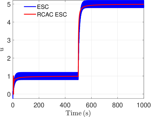
Figure 4: Example V.1:SISO Static map. Controller output $u$ for the static map given by (67) with ESC and RC/ESC. Note that the ESC response is shown in blue and the RC/ESC response is shown in red.

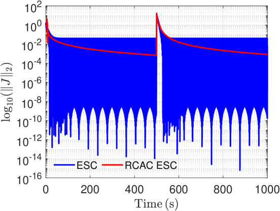
Figure 5: Example V.1:SISO Static map. Output error with respect to the optimal value $J=0$ in log scale with ESC and RC/ESC. Note that the error by ESC is shown in blue and the error by RC/ESC is shown in red.

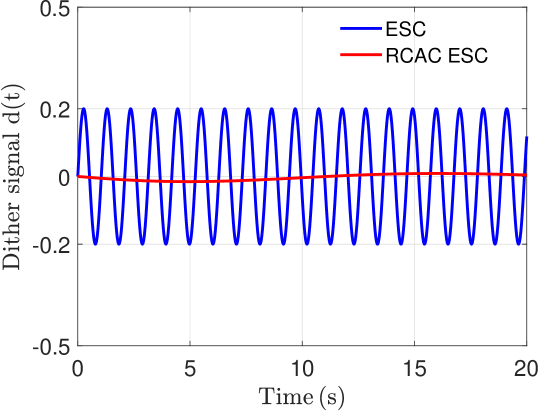
Figure 6: Example V.1:SISO Static map. Dither signal with ESC and RC/ESC. Note that the ESC dither signal is shown in blue and the RC/ESC dither signal is shown in red.

Example V.2

Static optimization in MISO system. Consider the static system

$$J(t_{=}(u_{(1)}(t)-r_{(1)}(t))^{2}+(u_{(2)}(t)-r_{(2)}(t))^{2}$$ (68)

where, for $t\in[0,500],$ $r(t)=\begin{bmatrix}1\\ 2\end{bmatrix},$ and for $t>500,$ $r(t)=\begin{bmatrix}-1\\ -2\end{bmatrix}.$ As mentioned in Section II, the objective is to minimize $J.$ Furthermore, the dither signals are shown in 9. The results of the numerical simulations are shown in Figures 7 and 8. While the response of RC/ESC converges to the minimizer in a slow manner, note that the response of RC/ESC doesn’t oscillate around the minimizer since the dither quickly goes to zero throughout the operation and eventually vanishes. $\diamond$

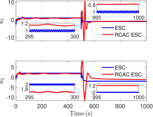
Figure 7: Example V.2:MISO Static map. Controller output components $u_{(1)}$ and $u_{(2)}$ for the static map given by (68) with ESC and RC/ESC. Note that the ESC response is shown in blue and the RC/ESC response is shown in red.

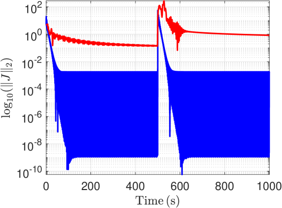
Figure 8: Example V.2:MISO Static map. Output error with respect to the optimal value $J=0$ in log scale with ESC and RC/ESC. Note that the error by ESC is shown in blue and the error by RC/ESC is shown in red.

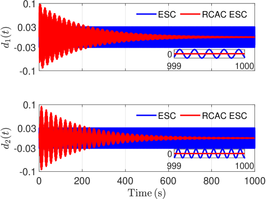
Figure 9: Example V.2:MISO Static map. Dither signals with ESC and RC/ESC. Note that the ESC dither signals are shown in blue and the RC/ESC dither signals are shown in red.

Example V.3

Dynamic optimization in MISO system (control gain tuning for stabilization).

Consider the Van Der Pol system

$$\ddot{x}+x+(\dot{x}^{2}-1)\dot{x}=u,$$ (69)

where $x_{1}=x$ and $x_{2}=\dot{x}$. Also, consider the full-state feedback controller structure given by

$$u=\begin{bmatrix}K_{1}&K_{2}\end{bmatrix}\begin{bmatrix}x_{1}\\ x_{2}\end{bmatrix}.$$ (70)

Also, an amplitude detector scheme is considered using moving standard deviation for each state and adding them along the entire horizon. Thus, the cost function $J$ is the amplitude of the oscillations of the states and ESC and RCAC-ESC are used to find suitable values of $\begin{bmatrix}K_{1}&K_{2}\end{bmatrix}$ in such a way that $J=0$ and thus, the system could be asymptotically stabilized. As mentioned in Section II, the objective is to minimize $J.$ Furthermore, the dither signals are shown in 13. The results of the numerical simulations are shown in Figures 10, 11 and 12. Both ESC and RC/ESC yield values of $K_{1}$ and $K_{2}$ that stabilize the response of the Van Der Pol system While the response of RC/ESC converges to the minimizer in a slow manner, note that the response of RC/ESC doesn’t oscillate around the minimizer since the dither quickly goes to zero throughout the operation and eventually vanishes. $\diamond$

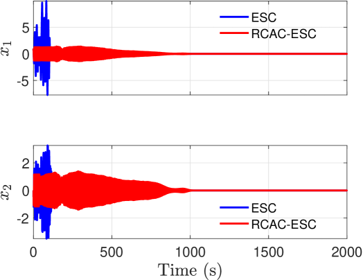
Figure 10: Example V.3:MISO Dynamic map. Components of the Van Der Pol system state $x$ versus time with ESC and RC/ESC. Note that the ESC result is shown in blue and the RC/ESC result is shown in red.

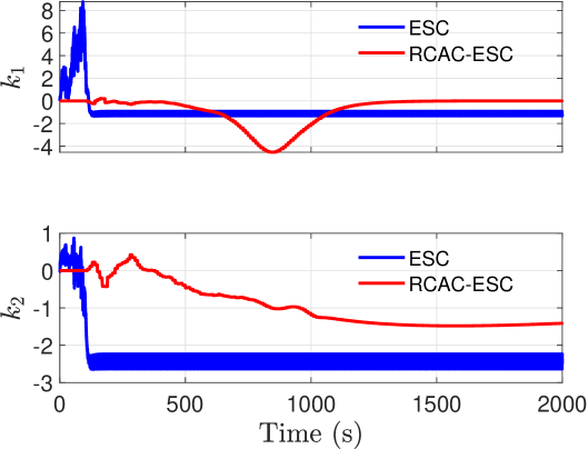
Figure 11: Example V.3:MISO Dynamic map. Controller gains $K_{1}$ and $K_{2}$ versus time with ESC and RC/ESC. Note that the ESC response is shown in blue and the RC/ESC response is shown in red

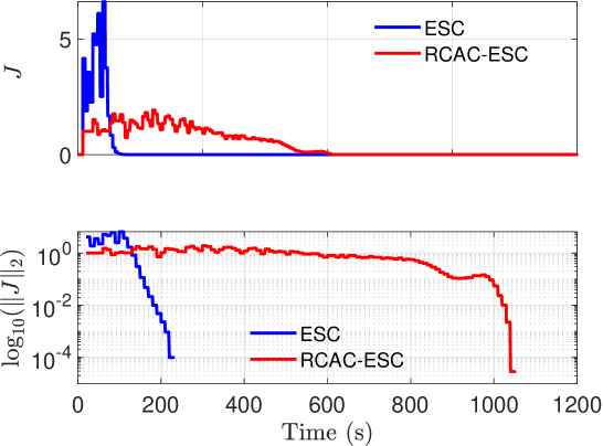
Figure 12: Example V.3: MISO Dynamic map. Output error with respect to the optimal value $J=0$ in regular and log scale with ESC and RC/ESC. Note that the error by ESC is shown in blue and the error by RC/ESC is shown in red.

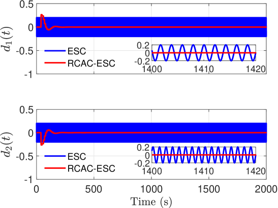
Figure 13: Example V.3: MISO Dynamic map. Dither signals with ESC and RC/ESC. Note that the ESC dither signals are shown in blue and the RC/ESC dither signals are shown in red.

VI Conclusions

This paper introduced a retrospective cost-based ESC controller for online output minimization with a vanishing perturbation. A KF is used to estimate the gradient of the system output at each step, which is then used to construct a target model that provides RCAC with a search direction to obtain a control input that minimizes the system output. Numerical examples illustrate the performance of this technique and provide a comparison with a regular continuous-time ESC scheme. Future work will focus on modifications for faster convergence and implementation in physical systems with time-varying minimizers.

References

• [1] K. B. Ariyur and M. Krstić, Real-Time Optimization by Extremum-Seeking Control.   John Wiley & Sons, 2003.
• [2] M. Krstić, “Performance improvement and limitations in extremum seeking control,” Systems & Control Letters, vol. 39, no. 5, pp. 313–326, 2000.
• [3] M. Krstić and H.-H. Wang, “Stability of extremum seeking feedback for general nonlinear dynamic systems,” Automatica, vol. 36, no. 4, pp. 595–601, 2000.
• [4] Y. Tan, W. H. Moase, C. Manzie, D. Nešić, and I. M. Mareels, “Extremum seeking from 1922 to 2010,” in Proc. Chin. Contr. Conf.   IEEE, 2010, pp. 14–26.
• [5] A. S. Matveev, H. Teimoori, and A. V. Savkin, “Navigation of a unicycle-like mobile robot for environmental extremum seeking,” Automatica, vol. 47, no. 1, pp. 85–91, 2011.
• [6] B. Calli, W. Caarls, P. Jonker, and M. Wisse, “Comparison of extremum seeking control algorithms for robotic applications,” in Proc. Int. Conf. Intell. Rob. Syst.   IEEE, 2012, pp. 3195–3202.
• [7] A. S. Matveev, M. C. Hoy, and A. V. Savkin, “3D environmental extremum seeking navigation of a nonholonomic mobile robot,” Automatica, vol. 50, no. 7, pp. 1802–1815, 2014.
• [8] A. O. Vweza, K. T. Chong, and D. J. Lee, “Gradient-free numerical optimization-based extremum seeking control for multiagent systems,” Int. J. Contro. Automat. Syst., vol. 13, no. 4, pp. 877–886, 2015.
• [9] A. S. Matveev, M. C. Hoy, and A. V. Savkin, “Extremum seeking navigation without derivative estimation of a mobile robot in a dynamic environmental field,” IEEE Trans. Contr. Syst. Tech., vol. 24, no. 3, pp. 1084–1091, 2015.
• [10] M. Bagheri, M. Krstić, and P. Naseradinmousavi, “Multivariable extremum seeking for joint-space trajectory optimization of a high-degrees-of-freedom robot,” J.f Dyn. Syst. Meas. Contr., vol. 140, no. 11, p. 111017, 2018.
• [11] B. Calli, W. Caarls, M. Wisse, and P. P. Jonker, “Active vision via extremum seeking for robots in unstructured environments: Applications in object recognition and manipulation,” IEEE Trans. Automat. Sci. Eng., vol. 15, no. 4, pp. 1810–1822, 2018.
• [12] F. E. Sotiropoulos and H. H. Asada, “A model-free extremum-seeking approach to autonomous excavator control based on output power maximization,” IEEE Robot. Automat. Lett., vol. 4, no. 2, pp. 1005–1012, 2019.
• [13] J. Creaby, Y. Li, and J. E. Seem, “Maximizing wind turbine energy capture using multivariable extremum seeking control,” Wind Eng., vol. 33, no. 4, pp. 361–387, 2009.
• [14] K. E. Johnson and G. Fritsch, “Assessment of extremum seeking control for wind farm energy production,” Wind Eng., vol. 36, no. 6, pp. 701–715, 2012.
• [15] A. Ghaffari, M. Krstić, and S. Seshagiri, “Power optimization and control in wind energy conversion systems using extremum seeking,” IEEE Trans. Contr. Syst. Tech., vol. 22, no. 5, pp. 1684–1695, 2014.
• [16] M. Ye and G. Hu, “Distributed extremum seeking for constrained networked optimization and its application to energy consumption control in smart grid,” IEEE Trans. Contr. Syst. Tech., vol. 24, no. 6, pp. 2048–2058, 2016.
• [17] N. Bizon, “Energy optimization of fuel cell system by using global extremum seeking algorithm,” Appl. Energy, vol. 206, pp. 458–474, 2017.
• [18] D. Zhou, A. Ravey, A. Al-Durra, and F. Gao, “A comparative study of extremum seeking methods applied to online energy management strategy of fuel cell hybrid electric vehicles,” Energy Conv. Manage., vol. 151, pp. 778–790, 2017.
• [19] D. Zhou, A. Al-Durra, I. Matraji, A. Ravey, and F. Gao, “Online energy management strategy of fuel cell hybrid electric vehicles: A fractional-order extremum seeking method,” IEEE Trans. Indust. Electr., vol. 65, no. 8, pp. 6787–6799, 2018.
• [20] L. Wang, S. Chen, and K. Ma, “On stability and application of extremum seeking control without steady-state oscillation,” Automatica, vol. 68, pp. 18–26, 2016.
• [21] M. Haring and T. A. Johansen, “Asymptotic stability of perturbation-based extremum-seeking control for nonlinear plants,” IEEE Trans. Autom. Contr., vol. 62, no. 5, pp. 2302–2317, 2016.
• [22] ——, “On the accuracy of gradient estimation in extremum-seeking control using small perturbations,” Automatica, vol. 95, pp. 23–32, 2018.
• [23] C. Yin, S. Dadras, X. Huang, Y. Chen, and S. Zhong, “Optimizing energy consumption for lighting control system via multivariate extremum seeking control with diminishing dither signal,” Trans. Automat. Sci. Eng., vol. 16, no. 4, pp. 1848–1859, 2019.
• [24] D. Bhattacharjee and K. Subbarao, “Extremum seeking control with attenuated steady-state oscillations,” Automatica, vol. 125, p. 109432, 2021.
• [25] Y. Rahman, A. Xie, and D. S. Bernstein, “Retrospective Cost Adaptive Control: Pole Placement, Frequency Response, and Connections with LQG Control,” IEEE Contr. Sys. Mag., vol. 37, pp. 28–69, Oct. 2017.
• [26] A. Goel and D. S. Bernstein, “Gradient-, Ensemble-, and Adjoint-Free Data-Driven Parameter Estimation,” J. Guid. Contr. Dyn., vol. 42, no. 8, pp. 1743–1754, 2019.
• [27] ——, “Retrospective cost parameter estimation with application to space weather modeling,” Handbook of Dynamic Data Driven Applications Systems: Volume 2, pp. 603–625, 2023.
• [28] J. Paredes, R. Ramesh, S. Obidov, M. Gamba, and D. Bernstein, “Experimental investigation of adaptive feedback control on a dual-swirl-stabilized gas turbine model combustor,” in AIAA Prop. Energy Forum, 2022, p. 2058.
• [29] D. Nešić, “Extremum seeking control: Convergence analysis,” European Journal of Control, vol. 15, no. 3-4, pp. 331–347, 2009.
• [30] K. B. Ariyur and M. Krstic, Real-time optimization by extremum-seeking control.   John Wiley & Sons, 2003.
• [31] S. A. U. Islam, T. Nguyen, I. Kolmanovsky, and D. S. Bernstein, “Data-Driven Retrospective Cost Adaptive Control for Flight Control Applications,” J. Guid. Contr. Dyn., vol. 44, pp. 1732–1758, October 2021.
• [32] L. Ljung and T. Soderstrom, Theory and Practice of Recursive Identification.   MIT Press, 1983.
• [33] S. A. U. Islam and D. S. Bernstein, “Recursive least squares for real-time implementation,” IEEE Contr. Syst. Mag., vol. 39, no. 3, pp. 82–85, 2019.
• [34] G. Gelbert, J. P. Moeck, C. O. Paschereit, and R. King, “Advanced algorithms for gradient estimation in one-and two-parameter extremum seeking controllers,” J. Proc. Contr., vol. 22, no. 4, pp. 700–709, 2012.