Measurement of $C\!P$ asymmetries in $B^{0}\rightarrow\mathit{{\eta}{}_{\mspace{-3.0mu}\scriptstyle{}}^{\mspace{-1.0mu}\scriptstyle{\prime}}}K^{0}_{\rm\scriptscriptstyle\textsl{S}}$ decays at Belle II

Abstract

We describe a measurement of charge-parity ($C\!P$) violation asymmetries in $B^{0}\rightarrow\mathit{{\eta}{}_{\mspace{-3.0mu}\scriptstyle{}}^{\mspace{-1.0mu}\scriptstyle{\prime}}}K^{0}_{\rm\scriptscriptstyle\textsl{S}}$ decays using Belle II data. We consider $\mathit{{\eta}{}_{\mspace{-3.0mu}\scriptstyle{}}^{\mspace{-1.0mu}\scriptstyle{\prime}}}\rightarrow\eta(\rightarrow\mathit{{\gamma}{}_{\mspace{-3.0mu}\scriptstyle{}}^{\mspace{-1.0mu}\scriptstyle{}}}\mathit{{\gamma}{}_{\mspace{-3.0mu}\scriptstyle{}}^{\mspace{-1.0mu}\scriptstyle{}}})\mathit{{\pi}{}_{\mspace{-3.0mu}\scriptstyle{}}^{\mspace{-1.0mu}\scriptstyle{+}}}\mathit{{\pi}{}_{\mspace{-3.0mu}\scriptstyle{}}^{\mspace{-1.0mu}\scriptstyle{-}}}$ and $\mathit{{\eta}{}_{\mspace{-3.0mu}\scriptstyle{}}^{\mspace{-1.0mu}\scriptstyle{\prime}}}\rightarrow\rho(\rightarrow\mathit{{\pi}{}_{\mspace{-3.0mu}\scriptstyle{}}^{\mspace{-1.0mu}\scriptstyle{+}}}\mathit{{\pi}{}_{\mspace{-3.0mu}\scriptstyle{}}^{\mspace{-1.0mu}\scriptstyle{-}}})\mathit{{\gamma}{}_{\mspace{-3.0mu}\scriptstyle{}}^{\mspace{-1.0mu}\scriptstyle{}}}$ decays. The data were collected at the SuperKEKB asymmetric-energy $e^{+}e^{-}$ collider between the years 2019 and 2022, and contain $(387\pm 6)\times 10^{6}$ bottom-antibottom meson pairs. We reconstruct $829\pm 35$ signal decays and extract the $C\!P$ violating parameters from a fit to the distribution of the proper-decay-time difference between the two $B$ mesons. The measured direct and mixing-induced $C\!P$ asymmetries are $C_{\mathit{{\eta}{}_{\mspace{-3.0mu}\scriptstyle{}}^{\mspace{-1.0mu}\scriptstyle{\prime}}}\!K^{0}_{\rm\scriptscriptstyle\textsl{S}}}=-0.19\pm 0.08\pm 0.03$ and $S_{\mathit{{\eta}{}_{\mspace{-3.0mu}\scriptstyle{}}^{\mspace{-1.0mu}\scriptstyle{\prime}}}\!K^{0}_{\rm\scriptscriptstyle\textsl{S}}}=+0.67\pm 0.10\pm 0.04$, respectively, where the first uncertainties are statistical and the second are systematic. These results are in agreement with current world averages and standard model predictions.

I Introduction

In the standard model (SM), the only source of charge-parity ($C\!P$) violation is an irreducible phase in the Cabibbo-Kobayashi-Maskawa (CKM) quark-mixing matrix Cabibbo (1963); Kobayashi and Maskawa (1973). This phase is measured with high precision in tree-dominated $b\rightarrow{c\bar{c}s}$ decays Adachi et al. (2012); Aubert et al. (2009a); Aaij et al. (2015), e.g., $B^{0}\rightarrow\mathit{{J\mspace{-2.0mu}/\mspace{-2.0mu}\psi}{}_{\mspace{-3.0mu}\scriptstyle{}}^{\mspace{-1.0mu}\scriptstyle{}}}K^{0}$. In contrast, $b\rightarrow{s}q\bar{q}$ decays, with $q$ indicating $u$, $d$, or $s$ quark, are dominated by loop amplitudes, in which additional sources of $C\!P$ violation from physics beyond the SM could be involved Altmannshofer et al. (2019); Ed. A. J. Bevan, B. Golob, Th. Mannel, S. Prell, and B. D. Yabsley (2014). A comparison between $C\!P$ asymmetries measured precisely in $b\rightarrow{s}q\bar{q}$ and $b\rightarrow{c\bar{c}s}$ transitions can thus probe non-SM physics.

The $B^{0}\rightarrow\mathit{{\eta}{}_{\mspace{-3.0mu}\scriptstyle{}}^{\mspace{-1.0mu}\scriptstyle{\prime}}}K^{0}_{\rm\scriptscriptstyle\textsl{S}}$ decay is of particular interest due to its relatively large branching fraction and limited contribution from tree amplitudes compared to other $b\rightarrow{s}q\bar{q}$ decays. The deviation of the mixing-induced $C\!P$ asymmetry ($S_{\mathit{{\eta}{}_{\mspace{-3.0mu}\scriptstyle{}}^{\mspace{-1.0mu}\scriptstyle{\prime}}}\!K^{0}_{\rm\scriptscriptstyle\textsl{S}}}$) from $\sin 2\phi_{1}$ is expected to be $0.01\pm 0.01$ Beneke (2005), in the SM, where $\phi_{1}\equiv\arg{(-V_{cd}V^{*}_{cb}/V_{td}V^{*}_{tb})}$ is an angle of the CKM unitarity triangle and $V_{ij}$ are the CKM matrix elements. The direct $C\!P$ asymmetry ($C_{\mathit{{\eta}{}_{\mspace{-3.0mu}\scriptstyle{}}^{\mspace{-1.0mu}\scriptstyle{\prime}}}\!K^{0}_{\rm\scriptscriptstyle\textsl{S}}}$) is predicted to be zero pdg .

Measurements of $C_{\mathit{{\eta}{}_{\mspace{-3.0mu}\scriptstyle{}}^{\mspace{-1.0mu}\scriptstyle{\prime}}}\!K^{0}_{\rm\scriptscriptstyle\textsl{S}}}$ and $S_{\mathit{{\eta}{}_{\mspace{-3.0mu}\scriptstyle{}}^{\mspace{-1.0mu}\scriptstyle{\prime}}}\!K^{0}_{\rm\scriptscriptstyle\textsl{S}}}$ have been reported by the Belle Šantelj et al. (2014) and BaBar Aubert et al. (2009b) experiments, yielding the current world averages $C_{\mathit{{\eta}{}_{\mspace{-3.0mu}\scriptstyle{}}^{\mspace{-1.0mu}\scriptstyle{\prime}}}\!K^{0}_{\rm\scriptscriptstyle\textsl{S}}}=-0.05\pm 0.04$ and $S_{\mathit{{\eta}{}_{\mspace{-3.0mu}\scriptstyle{}}^{\mspace{-1.0mu}\scriptstyle{\prime}}}\!K^{0}_{\rm\scriptscriptstyle\textsl{S}}}=0.63\pm 0.06$ Amhis et al. (2023). These are the most precise measurements of $C\!P$ asymmetries with $b\rightarrow sq\bar{q}$ transitions. However, improved measurements are needed to match the precision of the theoretical prediction of possible deviations from the SM Beneke (2005). The sensitivity of experiments operating at hadron colliders, such as LHCb, is limited by the challenge of the reconstruction of neutral final-state particles.

At an $e^{+}e^{-}$ flavor-factory, $B^{0}\kern 1.79993pt\overline{\kern-1.79993ptB}{}^{0}$ pairs are produced via the process $e^{+}e^{-}\rightarrow\Upsilon(4\mathrm{S})\rightarrow B^{0}\kern 1.79993pt\overline{\kern-1.79993ptB}{}^{0}$. We consider the case when one neutral $B$ meson (${B}_{\text{tag}}$) decays into a flavor-specific final state at time $t_{\text{tag}}$, and the other $B$ (${B}_{\textsl{CP}}$) decays into a $C\!P$ eigenstate at time $t_{\textsl{CP}}$. As the two neutral $B$ mesons remain in a quantum-entangled state until one of them decays, the flavor of ${B}_{\textsl{CP}}$ is opposite to that of ${B}_{\text{tag}}$ at $t_{\text{tag}}$. We define $q_{\mathrm{tag}}$ as the flavor of ${B}_{\text{tag}}$ at $t_{\text{tag}}$, with $q_{\mathrm{tag}}$ taking the value $+1\;(-1)$ for $B^{0}$ ($\kern 1.79993pt\overline{\kern-1.79993ptB}{}^{0}$). The decay rate for the ${B}_{\textsl{CP}}$ can be given by

$$\mathcal{P}(\Delta{t},q_{\mathrm{tag}})=\frac{e^{-|\Delta{t}|/\tau_{B^{0}}}}{4\tau_{B^{0}}}\left[1+q_{\mathrm{tag}}\mathcal{A}_{C\!P}(\Delta{t})\right],$$ (1)

where $\Delta{t}=t_{\textsl{CP}}-t_{\text{tag}}$ is the proper-time difference between the ${B}_{\textsl{CP}}$ and ${B}_{\text{tag}}$ decays, $\tau_{B^{0}}$ is the $B^{0}$ lifetime, and $\mathcal{A}_{C\!P}$ is the time-dependent $C\!P$ asymmetry, defined as

$$\begin{split}\mathcal{A}&{}_{C\!P}(\Delta{t})=\frac{\Gamma(\kern 1.79993pt\overline{\kern-1.79993ptB}{}^{0}\rightarrow\mathit{{\eta}{}_{\mspace{-3.0mu}\scriptstyle{}}^{\mspace{-1.0mu}\scriptstyle{\prime}}}K^{0}_{\rm\scriptscriptstyle\textsl{S}})-\Gamma(B^{0}\rightarrow\mathit{{\eta}{}_{\mspace{-3.0mu}\scriptstyle{}}^{\mspace{-1.0mu}\scriptstyle{\prime}}}K^{0}_{\rm\scriptscriptstyle\textsl{S}})}{\Gamma(\kern 1.79993pt\overline{\kern-1.79993ptB}{}^{0}\rightarrow\mathit{{\eta}{}_{\mspace{-3.0mu}\scriptstyle{}}^{\mspace{-1.0mu}\scriptstyle{\prime}}}K^{0}_{\rm\scriptscriptstyle\textsl{S}})+\Gamma(B^{0}\rightarrow\mathit{{\eta}{}_{\mspace{-3.0mu}\scriptstyle{}}^{\mspace{-1.0mu}\scriptstyle{\prime}}}K^{0}_{\rm\scriptscriptstyle\textsl{S}})}\\ &=S_{\mathit{{\eta}{}_{\mspace{-3.0mu}\scriptstyle{}}^{\mspace{-1.0mu}\scriptstyle{\prime}}}\!K^{0}_{\rm\scriptscriptstyle\textsl{S}}}\sin(\Delta{m_{d}}\Delta{t})-C_{\mathit{{\eta}{}_{\mspace{-3.0mu}\scriptstyle{}}^{\mspace{-1.0mu}\scriptstyle{\prime}}}\!K^{0}_{\rm\scriptscriptstyle\textsl{S}}}\cos(\Delta{m_{d}}\Delta{t}),\end{split}$$ (2)

where $\Delta{m_{d}}$ is the mass difference between the two neutral $B$-meson mass eigenstates.

This paper reports a measurement of $C\!P$ asymmetries $C_{\mathit{{\eta}{}_{\mspace{-3.0mu}\scriptstyle{}}^{\mspace{-1.0mu}\scriptstyle{\prime}}}\!K^{0}_{\rm\scriptscriptstyle\textsl{S}}}$ and $S_{\mathit{{\eta}{}_{\mspace{-3.0mu}\scriptstyle{}}^{\mspace{-1.0mu}\scriptstyle{\prime}}}\!K^{0}_{\rm\scriptscriptstyle\textsl{S}}}$, based on the data collected by the Belle II experiment in 2019–2022 at the SuperKEKB asymmetric-energy $e^{+}e^{-}$ collider Akai, Furukawa, and Koiso (2018), operating at the $\Upsilon(4\mathrm{S})$ resonance. The total integrated luminosity is $362\pm 2$$\mbox{\,fb}^{-1}$, which corresponds to $(387\pm 6)\text{\times}{10}^{6}$ $B\!\kern 1.79993pt\overline{\kern-1.79993ptB}{}$ pairs.

We reconstruct the signal decay (${B}_{\textsl{CP}}$) by combining the $K^{0}_{\rm\scriptscriptstyle\textsl{S}}\rightarrow\mathit{{\pi}{}_{\mspace{-3.0mu}\scriptstyle{}}^{\mspace{-1.0mu}\scriptstyle{+}}}\mathit{{\pi}{}_{\mspace{-3.0mu}\scriptstyle{}}^{\mspace{-1.0mu}\scriptstyle{-}}}$ candidate with the $\mathit{{\eta}{}_{\mspace{-3.0mu}\scriptstyle{}}^{\mspace{-1.0mu}\scriptstyle{\prime}}}$ meson reconstructed in two channels, $\mathit{{\eta}{}_{\mspace{-3.0mu}\scriptstyle{}}^{\mspace{-1.0mu}\scriptstyle{\prime}}}\rightarrow\eta(\rightarrow\gamma\gamma)\mathit{{\pi}{}_{\mspace{-3.0mu}\scriptstyle{}}^{\mspace{-1.0mu}\scriptstyle{+}}}\mathit{{\pi}{}_{\mspace{-3.0mu}\scriptstyle{}}^{\mspace{-1.0mu}\scriptstyle{-}}}$ and $\mathit{{\eta}{}_{\mspace{-3.0mu}\scriptstyle{}}^{\mspace{-1.0mu}\scriptstyle{\prime}}}\rightarrow\rho(\rightarrow\mathit{{\pi}{}_{\mspace{-3.0mu}\scriptstyle{}}^{\mspace{-1.0mu}\scriptstyle{+}}}\mathit{{\pi}{}_{\mspace{-3.0mu}\scriptstyle{}}^{\mspace{-1.0mu}\scriptstyle{-}}})\mathit{{\gamma}{}_{\mspace{-3.0mu}\scriptstyle{}}^{\mspace{-1.0mu}\scriptstyle{}}}$. We also explore the channel $\mathit{{\eta}{}_{\mspace{-3.0mu}\scriptstyle{}}^{\mspace{-1.0mu}\scriptstyle{\prime}}}\rightarrow\eta(\rightarrow\mathit{{\pi}{}_{\mspace{-3.0mu}\scriptstyle{}}^{\mspace{-1.0mu}\scriptstyle{-}}}\mathit{{\pi}{}_{\mspace{-3.0mu}\scriptstyle{}}^{\mspace{-1.0mu}\scriptstyle{+}}}\pi^{0})\mathit{{\pi}{}_{\mspace{-3.0mu}\scriptstyle{}}^{\mspace{-1.0mu}\scriptstyle{+}}}\mathit{{\pi}{}_{\mspace{-3.0mu}\scriptstyle{}}^{\mspace{-1.0mu}\scriptstyle{-}}}$, but exclude it from the final result due to its large statistical uncertainty. The ${B}_{\text{tag}}$ flavor is determined with a flavor tagging algorithm Abudinén et al. (2022). The values of $C_{\mathit{{\eta}{}_{\mspace{-3.0mu}\scriptstyle{}}^{\mspace{-1.0mu}\scriptstyle{\prime}}}\!K^{0}_{\rm\scriptscriptstyle\textsl{S}}}$ and $S_{\mathit{{\eta}{}_{\mspace{-3.0mu}\scriptstyle{}}^{\mspace{-1.0mu}\scriptstyle{\prime}}}\!K^{0}_{\rm\scriptscriptstyle\textsl{S}}}$ are extracted via a maximum-likelihood fit to the distributions of $\Delta{t}$ and other observables that discriminate signal from background. The analysis technique and the $\Delta{t}$ resolution model are tested on the $B^{+}\rightarrow\mathit{{\eta}{}_{\mspace{-3.0mu}\scriptstyle{}}^{\mspace{-1.0mu}\scriptstyle{\prime}}}\mathit{{K}{}_{\mspace{-3.0mu}\scriptstyle{}}^{\mspace{-1.0mu}\scriptstyle{+}}}$ control channel, where we do not expect any $C\!P$ violation. The measurement of the lifetimes of $B^{0}$ and $B^{+}$ mesons validates $\Delta{t}$ resolution modeling. Charge-conjugated modes are implied unless otherwise specified.

II Belle II detector and simulation

Belle II Abe et al. (2010) is a particle physics experiment operating at the SuperKEKB collider in Tsukuba, Japan. Several subsystems, cylindrically arranged around the interaction point, enable reconstruction of heavy flavor particles and $\tau$ leptons produced in energy-asymmetric $e^{+}e^{-}$ collisions. The innermost part of the detector comprises a two-layer silicon pixel detector (PXD), surrounded by a four-layer double-sided silicon microstrip detector (SVD). Together, they provide information about the charged particle trajectories (tracks) and $B$ decay positions (vertices). The momenta and charge of charged particles are reconstructed with a 56-layer central drift chamber (CDC), which is the main tracking subsystem. Only one sixth of the second PXD layer is installed for the data analyzed in this paper.

Charged particle identification (PID) is accomplished by a time-of-propagation counter and an aerogel ring-imaging Cherenkov counter, located in the barrel and forward-endcap regions, respectively. The CDC provides additional PID information through the measurement of specific ionization. An electromagnetic calorimeter (ECL), made of CsI(Tl) crystals, is used for precise determination of the photon energy and angular coordinates as well as for electron identification. The tracking, PID, and ECL subsystems are surrounded by a superconducting solenoid, providing an axial magnetic field of $1.5\,\text{T}$. A $K^{0}_{\rm\scriptscriptstyle\textsl{L}}$ and muon identification system is located outside of the magnet and consists of flux-return iron plates interspersed with resistive plate chambers and plastic scintillators. The central axis of the solenoid defines the $z$ axis of the laboratory frame, pointing approximately in the direction of the electron beam, with respect to which the polar angle $\theta$ is defined.

The analysis strategy is tested and optimized on Monte Carlo simulated event samples before being applied to the data. Simulation is also used to determine the signal efficiency and the fit model. Quark-antiquark pairs from $e^{+}e^{-}$ collisions are generated using KKMC Jadach, Ward, and Wa̧s (2000) with Pythia8 Sjöstrand et al. (2015), while hadron decays are simulated with EvtGen Lange (2001). The detector response and $K^{0}_{\rm\scriptscriptstyle\textsl{S}}$ decays are simulated using Geant4 Agostinelli et al. (2003). Both data and simulated samples are processed using the Belle II analysis software framework Kuhr et al. (2019); Belle II Collaboration (2022).

III Event reconstruction and selection

The reconstruction of signal candidates starts by reconstructing the $B^{0}$ decay products, $\mathit{{\eta}{}_{\mspace{-3.0mu}\scriptstyle{}}^{\mspace{-1.0mu}\scriptstyle{\prime}}}[\rightarrow\eta(\rightarrow{\mathit{{\gamma}{}_{\mspace{-3.0mu}\scriptstyle{}}^{\mspace{-1.0mu}\scriptstyle{}}}\mathit{{\gamma}{}_{\mspace{-3.0mu}\scriptstyle{}}^{\mspace{-1.0mu}\scriptstyle{}}}})\mathit{{\pi}{}_{\mspace{-3.0mu}\scriptstyle{}}^{\mspace{-1.0mu}\scriptstyle{+}}}\mathit{{\pi}{}_{\mspace{-3.0mu}\scriptstyle{}}^{\mspace{-1.0mu}\scriptstyle{-}}}]$, $\mathit{{\eta}{}_{\mspace{-3.0mu}\scriptstyle{}}^{\mspace{-1.0mu}\scriptstyle{\prime}}}[\rightarrow\rho(\rightarrow\mathit{{\pi}{}_{\mspace{-3.0mu}\scriptstyle{}}^{\mspace{-1.0mu}\scriptstyle{+}}}\mathit{{\pi}{}_{\mspace{-3.0mu}\scriptstyle{}}^{\mspace{-1.0mu}\scriptstyle{-}}})\mathit{{\gamma}{}_{\mspace{-3.0mu}\scriptstyle{}}^{\mspace{-1.0mu}\scriptstyle{}}}]$, and $K^{0}_{\rm\scriptscriptstyle\textsl{S}}\rightarrow\mathit{{\pi}{}_{\mspace{-3.0mu}\scriptstyle{}}^{\mspace{-1.0mu}\scriptstyle{+}}}\mathit{{\pi}{}_{\mspace{-3.0mu}\scriptstyle{}}^{\mspace{-1.0mu}\scriptstyle{-}}}$.

Charged particles, assumed to be pions, are reconstructed using the tracking algorithm described in Ref. Bertacchi et al. (2021), with measurement points from tracking subdetectors (PXD, SVD, and CDC). Pions are required to be within the CDC angular acceptance ($17^{\circ}<\theta<150^{\circ}$) and to have a distance of closest approach from the interaction point less than 2.0 cm along the $z$ axis and less than 0.5 cm in the transverse plane, in order to reduce contamination from tracks not produced in the collision. Furthermore, at least one of the two charged pions from $\mathit{{\eta}{}_{\mspace{-3.0mu}\scriptstyle{}}^{\mspace{-1.0mu}\scriptstyle{\prime}}}$ or $\rho$, which are used to reconstruct the ${B}_{\textsl{CP}}$ decay vertex, is required to have at least one PXD measurement point.

The photons are reconstructed from ECL energy deposits not associated to any track. They are required to be in the CDC angular acceptance and have energy deposit in more than one ECL crystal.

The $K^{0}_{\rm\scriptscriptstyle\textsl{S}}$ candidates are reconstructed from two oppositely charged pions coming from the same vertex and required to have a momentum direction compatible with the direction defined by the $K^{0}_{\rm\scriptscriptstyle\textsl{S}}$ and ${B}_{\textsl{CP}}$ decay vertices ($\cos\alpha>0.99$, where $\alpha$ is the angle between the two directions) and have an invariant mass $0.49<m(\mathit{{\pi}{}_{\mspace{-3.0mu}\scriptstyle{}}^{\mspace{-1.0mu}\scriptstyle{+}}}\mathit{{\pi}{}_{\mspace{-3.0mu}\scriptstyle{}}^{\mspace{-1.0mu}\scriptstyle{-}}})<0.51{\mathrm{\,Ge\kern-1.00006ptV\!/}c^{2}}$.

For the first decay subchannel, the $\eta\rightarrow\mathit{{\gamma}{}_{\mspace{-3.0mu}\scriptstyle{}}^{\mspace{-1.0mu}\scriptstyle{}}}\mathit{{\gamma}{}_{\mspace{-3.0mu}\scriptstyle{}}^{\mspace{-1.0mu}\scriptstyle{}}}$ candidates are reconstructed from two photons with energies greater than $150\,\mathrm{\,Me\kern-1.00006ptV}$ and an invariant mass in the range $0.505<m(\gamma\gamma)<0.580{\mathrm{\,Ge\kern-1.00006ptV\!/}c^{2}}$. The candidate $\eta$ and two oppositely charged pions are combined to form an $\mathit{{\eta}{}_{\mspace{-3.0mu}\scriptstyle{}}^{\mspace{-1.0mu}\scriptstyle{\prime}}}$, which is retained if its mass satisfies $0.945<m(\eta\mathit{{\pi}{}_{\mspace{-3.0mu}\scriptstyle{}}^{\mspace{-1.0mu}\scriptstyle{+}}}\mathit{{\pi}{}_{\mspace{-3.0mu}\scriptstyle{}}^{\mspace{-1.0mu}\scriptstyle{-}}})<0.970{\mathrm{\,Ge\kern-1.00006ptV\!/}c^{2}}$. The $\eta$ mass is constrained to its known value to reconstruct the $\mathit{{\eta}{}_{\mspace{-3.0mu}\scriptstyle{}}^{\mspace{-1.0mu}\scriptstyle{\prime}}}$ candidate.

For $\mathit{{\eta}{}_{\mspace{-3.0mu}\scriptstyle{}}^{\mspace{-1.0mu}\scriptstyle{\prime}}}\rightarrow\rho\mathit{{\gamma}{}_{\mspace{-3.0mu}\scriptstyle{}}^{\mspace{-1.0mu}\scriptstyle{}}}$ subchannel, we require two charged pions to first form a $\rho$ candidate. For this subchannel, the pions are required to satisfy a PID requirement, computed using all PID capable detectors, which has a $\mathit{{\pi}{}_{\mspace{-3.0mu}\scriptstyle{}}^{\mspace{-1.0mu}\scriptstyle{\pm}}}$ identification efficiency of about 90%, and a $\mathit{{K}{}_{\mspace{-3.0mu}\scriptstyle{}}^{\mspace{-1.0mu}\scriptstyle{\pm}}}$ mis-identification probability of about 10%. The pion tracks are also required to have at least 20 measurement points in the CDC, which is sufficient to provide high efficiency and a low rate of misreconstructed tracks. The tighter selection for the pions in the second subchannel helps to reduce the larger background as well as the number of misreconstructed signal candidates. A less restrictive requirement is applied on the dipion mass, due to the broad width of the $\rho$ resonance: $0.51<m(\mathit{{\pi}{}_{\mspace{-3.0mu}\scriptstyle{}}^{\mspace{-1.0mu}\scriptstyle{+}}}\mathit{{\pi}{}_{\mspace{-3.0mu}\scriptstyle{}}^{\mspace{-1.0mu}\scriptstyle{-}}})<1.0{\mathrm{\,Ge\kern-1.00006ptV\!/}c^{2}}$. The lower bound of the invariant mass criterion avoids contamination from $K^{0}_{\rm\scriptscriptstyle\textsl{S}}$ decays. An $\mathit{{\eta}{}_{\mspace{-3.0mu}\scriptstyle{}}^{\mspace{-1.0mu}\scriptstyle{\prime}}}$ candidate is formed combining a $\rho$ and a photon candidate with energy greater than 250$\mathrm{\,Me\kern-1.00006ptV}$. We require the invariant mass to be in the range $0.92<m(\rho\mathit{{\gamma}{}_{\mspace{-3.0mu}\scriptstyle{}}^{\mspace{-1.0mu}\scriptstyle{}}})<0.98{\mathrm{\,Ge\kern-1.00006ptV\!/}c^{2}}$. This subchannel has broader $\mathit{{\eta}{}_{\mspace{-3.0mu}\scriptstyle{}}^{\mspace{-1.0mu}\scriptstyle{\prime}}}$ mass resolution due to lack of constraint of $\rho$ mass.

The invariant mass criteria for the $\eta$, $\mathit{{\eta}{}_{\mspace{-3.0mu}\scriptstyle{}}^{\mspace{-1.0mu}\scriptstyle{\prime}}}$, and $K^{0}_{\rm\scriptscriptstyle\textsl{S}}$ candidates correspond to approximately $\pm 1.7\sigma_{m}$ intervals, where $\sigma_{m}$ is the Gaussian mass resolution of each decay mode.

The $\mathit{{\eta}{}_{\mspace{-3.0mu}\scriptstyle{}}^{\mspace{-1.0mu}\scriptstyle{\prime}}}$ and $K^{0}_{\rm\scriptscriptstyle\textsl{S}}$ candidates are combined to form a $B^{0}$ candidate. The $B^{0}$ vertex is determined by fitting the entire decay chain with the TreeFitter algorithm Krohn et al. (2020); Hulsbergen (2005), constraining the mass of all intermediate mesons to their known values Workman et al. (2022), except for the $\rho$, due to its large width, and requiring the fit to converge. The momenta of all particles are updated after this vertex fit. The $B^{0}$ vertex is constrained to point back, along the direction of the reconstructed $B^{0}$ momentum, to the interaction region, calibrated with $e^{+}e^{-}\rightarrow\mu^{+}\mu^{-}$.

For each $B$ candidate, the beam-energy constrained mass $M_{\text{bc}}=\sqrt{E^{*2}_{\text{beam}}/c^{4}-p^{*2}_{B}/c^{2}}$ and energy difference $\Delta{E}=E^{*}_{B}-E^{*}_{\text{beam}}$ are calculated, where $(E,p)^{*}_{B}$ is the four-momentum of the $B$ candidate and $E^{*}_{\text{beam}}$ is the beam energy, both calculated in the center-of-mass frame. For correctly reconstructed signal events, $M_{\text{bc}}$ peaks at the $B^{0}$ invariant mass and $\Delta{E}$ at zero. The requirements $M_{\text{bc}}>5.20\leavevmode\nobreak\ {\mathrm{\,Ge\kern-1.00006ptV\!/}c^{2}}$ and $|\Delta{E}|<0.2\leavevmode\nobreak\ \mathrm{\,Ge\kern-1.00006ptV}$ are applied.

In data, the average $B$ candidate multiplicity for events with at least one reconstructed candidate is about 1.4 for $B^{0}\rightarrow\mathit{{\eta}{}_{\mspace{-3.0mu}\scriptstyle{}}^{\mspace{-1.0mu}\scriptstyle{\prime}}}[\rightarrow\eta(\rightarrow\mathit{{\gamma}{}_{\mspace{-3.0mu}\scriptstyle{}}^{\mspace{-1.0mu}\scriptstyle{}}}\mathit{{\gamma}{}_{\mspace{-3.0mu}\scriptstyle{}}^{\mspace{-1.0mu}\scriptstyle{}}})\mathit{{\pi}{}_{\mspace{-3.0mu}\scriptstyle{}}^{\mspace{-1.0mu}\scriptstyle{+}}}\mathit{{\pi}{}_{\mspace{-3.0mu}\scriptstyle{}}^{\mspace{-1.0mu}\scriptstyle{-}}}]K^{0}_{\rm\scriptscriptstyle\textsl{S}}$ and 1.8 for $B^{0}\rightarrow\mathit{{\eta}{}_{\mspace{-3.0mu}\scriptstyle{}}^{\mspace{-1.0mu}\scriptstyle{\prime}}}[\rightarrow\rho\mathit{{\gamma}{}_{\mspace{-3.0mu}\scriptstyle{}}^{\mspace{-1.0mu}\scriptstyle{}}}]K^{0}_{\rm\scriptscriptstyle\textsl{S}}$. The difference is due to the presence of an intermediate, narrow resonance ($\eta$) in the first subchannel. If multiple $B$ candidates are present in an event, the one with the smallest $B^{0}$ vertex $\chi^{2}$ value is retained. In the simulation, this criterion selects the correct candidate in more than $99\%$ of the cases when a true one is reconstructed.

The reconstruction efficiencies, determined using simulation, are $28.3\%$ and $19.2\%$ for $B^{0}\rightarrow\mathit{{\eta}{}_{\mspace{-3.0mu}\scriptstyle{}}^{\mspace{-1.0mu}\scriptstyle{\prime}}}[\rightarrow\eta(\rightarrow\mathit{{\gamma}{}_{\mspace{-3.0mu}\scriptstyle{}}^{\mspace{-1.0mu}\scriptstyle{}}}\mathit{{\gamma}{}_{\mspace{-3.0mu}\scriptstyle{}}^{\mspace{-1.0mu}\scriptstyle{}}})\mathit{{\pi}{}_{\mspace{-3.0mu}\scriptstyle{}}^{\mspace{-1.0mu}\scriptstyle{+}}}\mathit{{\pi}{}_{\mspace{-3.0mu}\scriptstyle{}}^{\mspace{-1.0mu}\scriptstyle{-}}}]K^{0}_{\rm\scriptscriptstyle\textsl{S}}$ and $B^{0}\rightarrow\mathit{{\eta}{}_{\mspace{-3.0mu}\scriptstyle{}}^{\mspace{-1.0mu}\scriptstyle{\prime}}}[\rightarrow\rho\mathit{{\gamma}{}_{\mspace{-3.0mu}\scriptstyle{}}^{\mspace{-1.0mu}\scriptstyle{}}}]K^{0}_{\rm\scriptscriptstyle\textsl{S}}$, respectively. The lower efficiency for the second subchannel is mostly due to PID requirements applied to the two pions from the $\rho$ decay in order to suppress background.

The control channel $B^{+}\rightarrow\mathit{{\eta}{}_{\mspace{-3.0mu}\scriptstyle{}}^{\mspace{-1.0mu}\scriptstyle{\prime}}}\mathit{{K}{}_{\mspace{-3.0mu}\scriptstyle{}}^{\mspace{-1.0mu}\scriptstyle{+}}}$ uses an $\mathit{{\eta}{}_{\mspace{-3.0mu}\scriptstyle{}}^{\mspace{-1.0mu}\scriptstyle{\prime}}}$ reconstructed as described above and a charged kaon candidate with $\theta<136^{\circ}$, excluding candidates in the backward part of the detector, where the background is higher. The PID selection for the $\mathit{{K}{}_{\mspace{-3.0mu}\scriptstyle{}}^{\mspace{-1.0mu}\scriptstyle{+}}}$ candidate has an efficiency of about $90\%$ for kaons, and a misidentification probability for pions of about $5\%$. In the control channel, the $\mathit{{K}{}_{\mspace{-3.0mu}\scriptstyle{}}^{\mspace{-1.0mu}\scriptstyle{+}}}$ is not used for the $B^{+}$ vertex determination in order to have a vertex resolution similar to that of the signal channel.

The ${B}_{\text{tag}}$ candidate is reconstructed using all the charged particles that are not associated to ${B}_{\textsl{CP}}$, having measurement points both in the SVD and CDC, and a momenta greater than 50${\mathrm{\,Me\kern-1.00006ptV\!/}c}$. The RAVE algorithm is used to reconstruct the ${B}_{\text{tag}}$ vertex Waltenberger (2011). This algorithm downweights tracks with large contributions to the vertex $\chi^{2}$, which are likely to originate from decays of secondary long-lived charm hadrons. The decay position of ${B}_{\text{tag}}$ is determined by constraining its direction, as determined from its decay vertex and the interaction point, to be collinear with its momentum vector, reconstructed from the ${B}_{\textsl{CP}}$ and momenta of the colliding beams Dey and Soffer (2020).

The proper-decay-time difference $\Delta{t}$ between the two $B$ mesons is determined from the positions of their reconstructed vertices along the Lorentz boost axis, $\Delta{t}=\Delta{z}/\beta\gamma\gamma^{*}{c}$, where $\beta\gamma=0.287$ is the boost of the $\Upsilon(4\mathrm{S})$ with respect to the laboratory frame, and $\gamma^{*}=1.002$ is the Lorentz factor of the $B$ meson in the center-of-mass frame. We reject poorly reconstructed events requiring $|\Delta{t}|<8\leavevmode\nobreak\ \textrm{ps}$ and require the per-event uncertainty $\sigma_{\Delta{t}}$ to be less than $2\leavevmode\nobreak\ \textrm{ps}$.

The main source of background is random combinations of tracks and photons that arise from continuum $e^{+}e^{-}\rightarrow q\bar{q}$ ($q=u,d,s,c$) events. A boosted-decision-tree (BDT) classifier Keck (2017) is trained using 26 event-shape variables to separate jet-like continuum events from more spherical $B\!\kern 1.79993pt\overline{\kern-1.79993ptB}{}$ topologies. The variables, in order of decreasing discriminating power, are the cosine of the angle between the ${B}_{\textsl{CP}}$ and ${B}_{\text{tag}}$ thrust axes Brandt et al. (1964), the cosine of the angle between the ${B}_{\textsl{CP}}$ thrust axis and the $z$ axis, the ratio of the second to the zeroth Fox–Wolfram moments Fox and Wolfram (1978), the modified Fox–Wolfram moments Lee et al. (2003), the ${B}_{\text{tag}}$ thrust magnitude, and the CLEO cones Asner et al. (1996). Variables that exhibit correlations greater than 10% with those used for the $C\!P$ asymmetry measurement ($M_{\text{bc}}$, $\Delta{E}$, $\Delta{t}$, and $\sigma_{\Delta{t}}$) are excluded. The BDT training is performed using simulated signal events and data in the sidebands ($M_{\text{bc}}<5.27{\mathrm{\,Ge\kern-1.00006ptV\!/}c^{2}}$ and $\Delta{E}<-0.07$ or $>0.05\mathrm{\,Ge\kern-1.00006ptV}$), which are dominated by continuum background. As a consistency check, we repeat the training with the off-resonance data collected at an energy 60$\mathrm{\,Me\kern-1.00006ptV}$ below the $\Upsilon(4\mathrm{S})$ resonance, for an integrated luminosity of $42\leavevmode\nobreak\ \mbox{\,fb}^{-1}$, and find the results to be in agreement with those obtained with the nominal training. A high-efficiency selection on the BDT output $C_{\rm BDT}$ is applied, retaining about 95% of the signal while suppressing 60% of the continuum background.

IV Time-dependent $C\!P$ asymmetry fit

The parameters $C_{\mathit{{\eta}{}_{\mspace{-3.0mu}\scriptstyle{}}^{\mspace{-1.0mu}\scriptstyle{\prime}}}\!K^{0}_{\rm\scriptscriptstyle\textsl{S}}}$ and $S_{\mathit{{\eta}{}_{\mspace{-3.0mu}\scriptstyle{}}^{\mspace{-1.0mu}\scriptstyle{\prime}}}\!K^{0}_{\rm\scriptscriptstyle\textsl{S}}}$ are extracted with an extended unbinned maximum-likelihood fit using the $M_{\text{bc}}$, $\Delta{E}$, $C_{\rm BDT}$, $\Delta{t}$, and tag-flavor $q_{\mathrm{tag}}$ observables, plus $\sigma_{\Delta{t}}$ as a conditional observable for $\Delta{t}$ resolution function. The first three observables provide discrimination between signal and continuum background. The $\Delta{t}$ and $q_{\mathrm{tag}}$ ones provide access to time-dependent $C\!P$ asymmetry. Four different sample components are considered: signal; self-cross-feed (SxF), where a signal decay is misreconstructed, mostly due to wrong $\mathit{{\gamma}{}_{\mspace{-3.0mu}\scriptstyle{}}^{\mspace{-1.0mu}\scriptstyle{}}}$ associations; background from continuum; and background from $B\!\kern 1.79993pt\overline{\kern-1.79993ptB}{}$. The SxF sample amounts to about 5% of the signal while $B\!\kern 1.79993pt\overline{\kern-1.79993ptB}{}$ amounts to about 1% of the continuum.

The fit is performed in two steps. In the first step the shapes and yields of all sample components are reliably determined in a time-independent fit, using $M_{\text{bc}}$, $\Delta{E}$, and $C_{\rm BDT}$ distributions in the region $M_{\text{bc}}>5.2{\mathrm{\,Ge\kern-1.00006ptV\!/}c^{2}}$ and $|\Delta{E}|<0.2\mathrm{\,Ge\kern-1.00006ptV}$, which in turn simplify the time-dependent fit of the second step. In the first step most parameters of the signal and continuum models are allowed to vary, as well as the yields of signal and continuum. The SxF shape is fixed from simulated events, as well as its normalization relative to the signal component. The shape and yields of the $B\!\kern 1.79993pt\overline{\kern-1.79993ptB}{}$ component are fixed from simulation, as their contribution is too small to be determined from data.

The second step of the fit uses $\Delta{t}$ and $q_{\mathrm{tag}}$ in addition to the three observables utilized in the first step, and is performed only in the signal region, defined by $M_{\text{bc}}>5.27{\mathrm{\,Ge\kern-1.00006ptV\!/}c^{2}}$ and $-0.07<\Delta{E}<0.05\mathrm{\,Ge\kern-1.00006ptV}$, where approximately $98\%$ of signal is present. In this region the SxF amounts to about 3% of signal. In this step, the shapes for $M_{\text{bc}}$, $\Delta{E}$, and $C_{\rm BDT}$ as well as the yields of all components are fixed from the previous one, so the only free parameters are $C_{\mathit{{\eta}{}_{\mspace{-3.0mu}\scriptstyle{}}^{\mspace{-1.0mu}\scriptstyle{\prime}}}\!K^{0}_{\rm\scriptscriptstyle\textsl{S}}}$ and $S_{\mathit{{\eta}{}_{\mspace{-3.0mu}\scriptstyle{}}^{\mspace{-1.0mu}\scriptstyle{\prime}}}\!K^{0}_{\rm\scriptscriptstyle\textsl{S}}}$.

The ${B}_{\text{tag}}$ flavor is determined using the flavor tagging algorithm described in Ref. Abudinén et al. (2022), which uses the properties of particles not associated with the ${B}_{\textsl{CP}}$. The algorithm provides the flavor $q_{\mathrm{tag}}$ and the tagging quality $r=(1-2w)$, where $w$ is the mistagging probability. The range of $r$ varies from $r=0$ (no flavor information can be obtained) to $r=1$ (corresponding to unambiguous determination of the flavor).

Both fit steps are performed simultaneously in seven subsets of data (bins) selected according to tagging quality $r$, with boundaries set at 0, 0.1, 0.25, 0.45, 0.6, 0.725, 0.875, and 1, to gain statistical sensitivity from events with different wrong-tag fractions. In the first step, the signal and continuum yields of each bin are varied independently.

Each observable is modeled independently and hence the total probability density function (PDF) is the product of the four independent PDFs. The correlation between $M_{\text{bc}}$ and $\Delta{E}$ (10% and 20% for the two subchannels, respectively), due to the presence of photons in the final state, is considered as a source of systematic uncertainty.

The $M_{\text{bc}}$ distribution is modeled with a sum of two Gaussian functions with a common mean for signal, a Crystal Ball function Gaiser (1982); Skwarnicki (1986); Oreglia et al. (1982) for SxF, an ARGUS function Albrecht et al. (1990) for continuum, and an ARGUS plus a Gaussian function for $B\!\kern 1.79993pt\overline{\kern-1.79993ptB}{}$. In the case of $\Delta{E}$, two Gaussian functions are used for signal and SxF, with the addition of a linear function for $B^{0}\rightarrow\mathit{{\eta}{}_{\mspace{-3.0mu}\scriptstyle{}}^{\mspace{-1.0mu}\scriptstyle{\prime}}}[\rightarrow\rho\mathit{{\gamma}{}_{\mspace{-3.0mu}\scriptstyle{}}^{\mspace{-1.0mu}\scriptstyle{}}}]K^{0}_{\rm\scriptscriptstyle\textsl{S}}$. For continuum, we use an exponential for $B^{0}\rightarrow\mathit{{\eta}{}_{\mspace{-3.0mu}\scriptstyle{}}^{\mspace{-1.0mu}\scriptstyle{\prime}}}(\rightarrow\eta(\rightarrow\mathit{{\gamma}{}_{\mspace{-3.0mu}\scriptstyle{}}^{\mspace{-1.0mu}\scriptstyle{}}}\mathit{{\gamma}{}_{\mspace{-3.0mu}\scriptstyle{}}^{\mspace{-1.0mu}\scriptstyle{}}})\mathit{{\pi}{}_{\mspace{-3.0mu}\scriptstyle{}}^{\mspace{-1.0mu}\scriptstyle{+}}}\mathit{{\pi}{}_{\mspace{-3.0mu}\scriptstyle{}}^{\mspace{-1.0mu}\scriptstyle{-}}})K^{0}_{\rm\scriptscriptstyle\textsl{S}}\leavevmode\nobreak\$ and the sum of an exponential and a wide Gaussian function for $B^{0}\rightarrow\mathit{{\eta}{}_{\mspace{-3.0mu}\scriptstyle{}}^{\mspace{-1.0mu}\scriptstyle{\prime}}}[\rightarrow\rho\mathit{{\gamma}{}_{\mspace{-3.0mu}\scriptstyle{}}^{\mspace{-1.0mu}\scriptstyle{}}}]K^{0}_{\rm\scriptscriptstyle\textsl{S}}$. For $B\!\kern 1.79993pt\overline{\kern-1.79993ptB}{}$, we use an exponential plus a Gaussian function. For $C_{\rm BDT}$, the sum of an asymmetric and a regular Gaussian function is used for signal, SxF, and $B\!\kern 1.79993pt\overline{\kern-1.79993ptB}{}$, and two Gaussian functions for continuum.

The $\Delta{t}$ model for the signal and SxF components is derived from Eq. 1. Taking into account the probability of assigning the wrong flavor, $w$, its difference between $B^{0}$ and $\kern 1.79993pt\overline{\kern-1.79993ptB}{}^{0}$, $\Delta{w}$, and the tagging efficiency asymmetry for $B^{0}$ and $\kern 1.79993pt\overline{\kern-1.79993ptB}{}^{0}$, $a_{\epsilon}^{\rm tag}$, Eq. 1 becomes

$$\begin{split}\mathcal{P}(&\Delta{t},q_{\mathrm{tag}})=\frac{e^{-|\Delta{t}|/\tau_{B^{0}}}}{4\tau_{B^{0}}}\Biggl{\{}1-q_{\mathrm{tag}}\Delta{w}+q_{\mathrm{tag}}a_{\epsilon}^{\rm tag}(1-2w)+\\ &\left[q_{\mathrm{tag}}(1-2w)+a_{\epsilon}^{\rm tag}(1-q_{\mathrm{tag}}\Delta{w})\right]\left[S_{\mathit{{\eta}{}_{\mspace{-3.0mu}\scriptstyle{}}^{\mspace{-1.0mu}\scriptstyle{\prime}}}\!K^{0}_{\rm\scriptscriptstyle\textsl{S}}}\sin(\Delta{m_{d}}\Delta{t})-C_{\mathit{{\eta}{}_{\mspace{-3.0mu}\scriptstyle{}}^{\mspace{-1.0mu}\scriptstyle{\prime}}}\!K^{0}_{\rm\scriptscriptstyle\textsl{S}}}\cos(\Delta{m_{d}}\Delta{t})\right]\Biggr{\}}.\\ \end{split}$$ (3)

The effect of detector resolution on $\Delta{t}$ changes Eq. 3 to

$$\mathcal{P}_{\rm exp}(\Delta{t},q_{\mathrm{tag}})=\int\mathcal{P}(\Delta{t^{\prime}},q_{\mathrm{tag}})\mathcal{R}(\Delta{t}-\Delta{t^{\prime}}|\sigma_{\Delta{t}})d\Delta{t^{\prime}},$$ (4)

where $\mathcal{R}$ is the resolution function for $\Delta{t}$ conditional on $\sigma_{\Delta{t}}$. The $\mathcal{R}$ function has been determined in data using $B^{0}\rightarrow D^{(*)-}\mathit{{\pi}{}_{\mspace{-3.0mu}\scriptstyle{}}^{\mspace{-1.0mu}\scriptstyle{+}}}$ decays and it is described in details in Ref. Abudinén et al. (2023). Like the resolution function, also the flavor tagging parameters $w$, $\Delta{w}$, and $a_{\epsilon}^{\rm tag}$ are extracted from data using flavor-specific $B^{0}\rightarrow D^{(*)-}\mathit{{\pi}{}_{\mspace{-3.0mu}\scriptstyle{}}^{\mspace{-1.0mu}\scriptstyle{+}}}$ decays. In simulation all these parameters from $B^{0}\rightarrow D^{(*)-}\mathit{{\pi}{}_{\mspace{-3.0mu}\scriptstyle{}}^{\mspace{-1.0mu}\scriptstyle{+}}}$ are compatible with our expectations based on signal.

The $\Delta{t}$ distribution for the continuum component is modeled with three Gaussian functions and is determined using the data sidebands described earlier. The $\Delta{t}$ distribution of the $B\!\kern 1.79993pt\overline{\kern-1.79993ptB}{}$ background is also modeled with the sum of three Gaussian functions and a component with an effective lifetime, that accounts for the sizable $B$ lifetime, convolved with the same three Gaussian functions. Its parameters are determined from simulation.

To validate the resolution function, we determine the $B$ meson’s lifetime on data, using a simultaneous fit to both $\mathit{{\eta}{}_{\mspace{-3.0mu}\scriptstyle{}}^{\mspace{-1.0mu}\scriptstyle{\prime}}}$ subchannels, separately for charged $B^{+}\rightarrow\mathit{{\eta}{}_{\mspace{-3.0mu}\scriptstyle{}}^{\mspace{-1.0mu}\scriptstyle{\prime}}}\mathit{{K}{}_{\mspace{-3.0mu}\scriptstyle{}}^{\mspace{-1.0mu}\scriptstyle{+}}}$ and neutral $B^{0}\rightarrow\mathit{{\eta}{}_{\mspace{-3.0mu}\scriptstyle{}}^{\mspace{-1.0mu}\scriptstyle{\prime}}}K^{0}_{\rm\scriptscriptstyle\textsl{S}}$ decays. The results are $\tau_{B^{+}}=1.63\pm 0.04{\rm\,ps}$ and $\tau_{B^{0}}=1.55\pm 0.07{\rm\,ps}$, where the uncertainties are statistical. Both are in agreement with their world averages Workman et al. (2022).

The fit is further validated measuring the $C\!P$ asymmetry on the charged $B$ decay, which is expected to be negligible, with a simultaneous fit to the two $\mathit{{\eta}{}_{\mspace{-3.0mu}\scriptstyle{}}^{\mspace{-1.0mu}\scriptstyle{\prime}}}$ subchannels. The same flavor tagger used for the neutral channels is used also for the control ones. In the signal region we find $1345\pm 39$ and $1694\pm 64$ signal events for $B^{+}\rightarrow\mathit{{\eta}{}_{\mspace{-3.0mu}\scriptstyle{}}^{\mspace{-1.0mu}\scriptstyle{\prime}}}[\rightarrow\eta(\rightarrow\mathit{{\gamma}{}_{\mspace{-3.0mu}\scriptstyle{}}^{\mspace{-1.0mu}\scriptstyle{}}}\mathit{{\gamma}{}_{\mspace{-3.0mu}\scriptstyle{}}^{\mspace{-1.0mu}\scriptstyle{}}})\mathit{{\pi}{}_{\mspace{-3.0mu}\scriptstyle{}}^{\mspace{-1.0mu}\scriptstyle{+}}}\mathit{{\pi}{}_{\mspace{-3.0mu}\scriptstyle{}}^{\mspace{-1.0mu}\scriptstyle{-}}}]\mathit{{K}{}_{\mspace{-3.0mu}\scriptstyle{}}^{\mspace{-1.0mu}\scriptstyle{+}}}$ and $B^{+}\rightarrow\mathit{{\eta}{}_{\mspace{-3.0mu}\scriptstyle{}}^{\mspace{-1.0mu}\scriptstyle{\prime}}}[\rightarrow\rho\mathit{{\gamma}{}_{\mspace{-3.0mu}\scriptstyle{}}^{\mspace{-1.0mu}\scriptstyle{}}}]\mathit{{K}{}_{\mspace{-3.0mu}\scriptstyle{}}^{\mspace{-1.0mu}\scriptstyle{+}}}$ subchannels with purities (which is the ratio of signal events over the total number of events in the signal region) $77\%$ and $24\%$, respectively. The resulting $C\!P$ violation parameters are $C_{\mathit{{\eta}{}_{\mspace{-3.0mu}\scriptstyle{}}^{\mspace{-1.0mu}\scriptstyle{\prime}}}\!\mathit{{K}{}_{\mspace{-3.0mu}\scriptstyle{}}^{\mspace{-1.0mu}\scriptstyle{+}}}}={-0.018\pm 0.044}$ and $S_{\mathit{{\eta}{}_{\mspace{-3.0mu}\scriptstyle{}}^{\mspace{-1.0mu}\scriptstyle{\prime}}}\!\mathit{{K}{}_{\mspace{-3.0mu}\scriptstyle{}}^{\mspace{-1.0mu}\scriptstyle{+}}}}=-0.083\pm 0.059$, where the uncertainties are statistical. The results are consistent with expectations of zero $C\!P$ asymmetry. The $\Delta{t}$ distributions are shown separately for $B$ and $\mathit{{\mkern 4.0mu\overline{\mkern-4.0mu{B}}}{}_{\mspace{-2.0mu}\scriptstyle{}}^{\mspace{0.0mu}\scriptstyle{}}}$ tagged events in Fig. 1, along with the asymmetry as defined in Eq. 2.

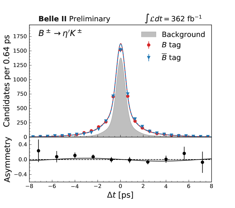
Figure 1: Distribution of $\Delta{t}$ for control channels $B^{+}\rightarrow\mathit{{\eta}{}_{\mspace{-3.0mu}\scriptstyle{}}^{\mspace{-1.0mu}\scriptstyle{\prime}}}\mathit{{K}{}_{\mspace{-3.0mu}\scriptstyle{}}^{\mspace{-1.0mu}\scriptstyle{+}}}$ separately for $B$ and $\mathit{{\mkern 4.0mu\overline{\mkern-4.0mu{B}}}{}_{\mspace{-2.0mu}\scriptstyle{}}^{\mspace{0.0mu}\scriptstyle{}}}$ tags, combining the two subchannels $B^{+}\rightarrow\mathit{{\eta}{}_{\mspace{-3.0mu}\scriptstyle{}}^{\mspace{-1.0mu}\scriptstyle{\prime}}}[\rightarrow\eta(\rightarrow\mathit{{\gamma}{}_{\mspace{-3.0mu}\scriptstyle{}}^{\mspace{-1.0mu}\scriptstyle{}}}\mathit{{\gamma}{}_{\mspace{-3.0mu}\scriptstyle{}}^{\mspace{-1.0mu}\scriptstyle{}}})\mathit{{\pi}{}_{\mspace{-3.0mu}\scriptstyle{}}^{\mspace{-1.0mu}\scriptstyle{+}}}\mathit{{\pi}{}_{\mspace{-3.0mu}\scriptstyle{}}^{\mspace{-1.0mu}\scriptstyle{-}}}]\mathit{{K}{}_{\mspace{-3.0mu}\scriptstyle{}}^{\mspace{-1.0mu}\scriptstyle{+}}}$and $B^{+}\rightarrow\mathit{{\eta}{}_{\mspace{-3.0mu}\scriptstyle{}}^{\mspace{-1.0mu}\scriptstyle{\prime}}}[\rightarrow\rho\mathit{{\gamma}{}_{\mspace{-3.0mu}\scriptstyle{}}^{\mspace{-1.0mu}\scriptstyle{}}}]\mathit{{K}{}_{\mspace{-3.0mu}\scriptstyle{}}^{\mspace{-1.0mu}\scriptstyle{+}}}$. The background contribution is also shown as a shaded area. The fit projections corresponding to $B$ ($q_{\mathrm{tag}}=1$) and $\mathit{{\mkern 4.0mu\overline{\mkern-4.0mu{B}}}{}_{\mspace{-2.0mu}\scriptstyle{}}^{\mspace{0.0mu}\scriptstyle{}}}$ ($q_{\mathrm{tag}}=-1$) tags are shown as solid red and dashed blue curves, respectively. The bottom panel shows the asymmetry as defined in Eq. 2, after subtracting the background using the ${{}_{s}Plot}$ technique Pivk and Le Diberder (2005).

We then apply the fit to our signal, the neutral $B$ samples. The distributions of the fit observables, $M_{\text{bc}}$, $\Delta{E}$, and $C_{\rm BDT}$ in the signal region are shown in Fig. 2 for the $B^{0}\rightarrow\mathit{{\eta}{}_{\mspace{-3.0mu}\scriptstyle{}}^{\mspace{-1.0mu}\scriptstyle{\prime}}}[\rightarrow\eta(\rightarrow\mathit{{\gamma}{}_{\mspace{-3.0mu}\scriptstyle{}}^{\mspace{-1.0mu}\scriptstyle{}}}\mathit{{\gamma}{}_{\mspace{-3.0mu}\scriptstyle{}}^{\mspace{-1.0mu}\scriptstyle{}}})\mathit{{\pi}{}_{\mspace{-3.0mu}\scriptstyle{}}^{\mspace{-1.0mu}\scriptstyle{+}}}\mathit{{\pi}{}_{\mspace{-3.0mu}\scriptstyle{}}^{\mspace{-1.0mu}\scriptstyle{-}}}]K^{0}_{\rm\scriptscriptstyle\textsl{S}}$ subchannel, and in Fig. 3 for $B^{0}\rightarrow\mathit{{\eta}{}_{\mspace{-3.0mu}\scriptstyle{}}^{\mspace{-1.0mu}\scriptstyle{\prime}}}[\rightarrow\rho\mathit{{\gamma}{}_{\mspace{-3.0mu}\scriptstyle{}}^{\mspace{-1.0mu}\scriptstyle{}}}]K^{0}_{\rm\scriptscriptstyle\textsl{S}}$ together with the fit results of the four components. The $\Delta{t}$ distributions are shown separately for $B^{0}$ and $\kern 1.79993pt\overline{\kern-1.79993ptB}{}^{0}$ tagged events in Figs. 4 and 5 for subchannels $B^{0}\rightarrow\mathit{{\eta}{}_{\mspace{-3.0mu}\scriptstyle{}}^{\mspace{-1.0mu}\scriptstyle{\prime}}}[\rightarrow\eta(\rightarrow\mathit{{\gamma}{}_{\mspace{-3.0mu}\scriptstyle{}}^{\mspace{-1.0mu}\scriptstyle{}}}\mathit{{\gamma}{}_{\mspace{-3.0mu}\scriptstyle{}}^{\mspace{-1.0mu}\scriptstyle{}}})\mathit{{\pi}{}_{\mspace{-3.0mu}\scriptstyle{}}^{\mspace{-1.0mu}\scriptstyle{+}}}\mathit{{\pi}{}_{\mspace{-3.0mu}\scriptstyle{}}^{\mspace{-1.0mu}\scriptstyle{-}}}]K^{0}_{\rm\scriptscriptstyle\textsl{S}}$ and $B^{0}\rightarrow\mathit{{\eta}{}_{\mspace{-3.0mu}\scriptstyle{}}^{\mspace{-1.0mu}\scriptstyle{\prime}}}[\rightarrow\rho\mathit{{\gamma}{}_{\mspace{-3.0mu}\scriptstyle{}}^{\mspace{-1.0mu}\scriptstyle{}}}]K^{0}_{\rm\scriptscriptstyle\textsl{S}}$, respectively, and in Fig. 6 for both, along with the asymmetry as defined in Eq. 2.

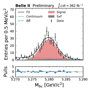
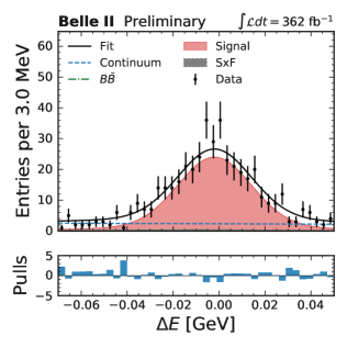
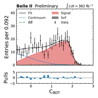
Figure 2: Distributions of $M_{\text{bc}}$, $\Delta{E}$, and $C_{\rm BDT}$ on data for $B^{0}\rightarrow\mathit{{\eta}{}_{\mspace{-3.0mu}\scriptstyle{}}^{\mspace{-1.0mu}\scriptstyle{\prime}}}[\rightarrow\eta(\rightarrow\mathit{{\gamma}{}_{\mspace{-3.0mu}\scriptstyle{}}^{\mspace{-1.0mu}\scriptstyle{}}}\mathit{{\gamma}{}_{\mspace{-3.0mu}\scriptstyle{}}^{\mspace{-1.0mu}\scriptstyle{}}})\mathit{{\pi}{}_{\mspace{-3.0mu}\scriptstyle{}}^{\mspace{-1.0mu}\scriptstyle{+}}}\mathit{{\pi}{}_{\mspace{-3.0mu}\scriptstyle{}}^{\mspace{-1.0mu}\scriptstyle{-}}}]K^{0}_{\rm\scriptscriptstyle\textsl{S}}$, with fit projections overlaid. The bottom panel shows the pull, which is the difference between data and fit, normalized to the statistical uncertainty on data.

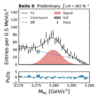
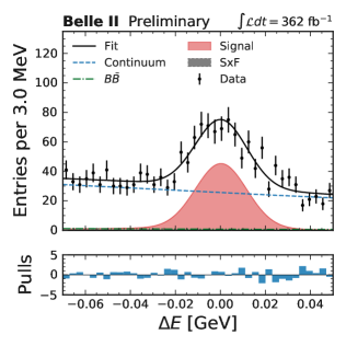
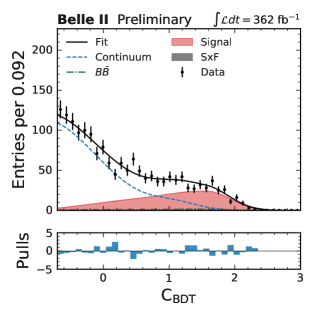
Figure 3: Distributions of $M_{\text{bc}}$, $\Delta{E}$, and $C_{\rm BDT}$ on data for $B^{0}\rightarrow\mathit{{\eta}{}_{\mspace{-3.0mu}\scriptstyle{}}^{\mspace{-1.0mu}\scriptstyle{\prime}}}[\rightarrow\rho\mathit{{\gamma}{}_{\mspace{-3.0mu}\scriptstyle{}}^{\mspace{-1.0mu}\scriptstyle{}}}]K^{0}_{\rm\scriptscriptstyle\textsl{S}}$, with fit projections overlaid. The bottom panel shows the pull.

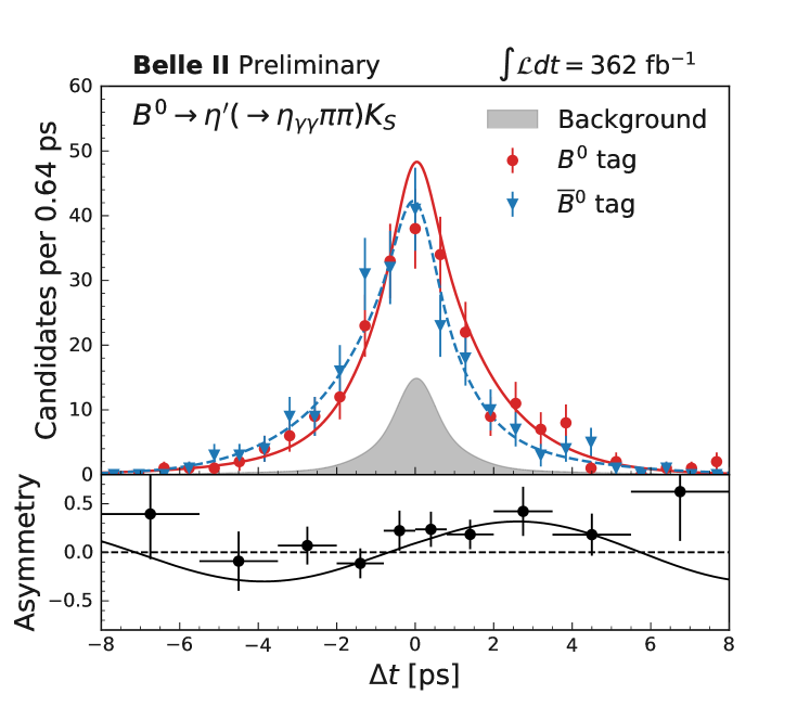
Figure 4: Distribution of $\Delta{t}$ for signal channels separately for $B^{0}$ and $\kern 1.79993pt\overline{\kern-1.79993ptB}{}^{0}$ tags, for $B^{0}\rightarrow\mathit{{\eta}{}_{\mspace{-3.0mu}\scriptstyle{}}^{\mspace{-1.0mu}\scriptstyle{\prime}}}[\rightarrow\eta(\rightarrow\mathit{{\gamma}{}_{\mspace{-3.0mu}\scriptstyle{}}^{\mspace{-1.0mu}\scriptstyle{}}}\mathit{{\gamma}{}_{\mspace{-3.0mu}\scriptstyle{}}^{\mspace{-1.0mu}\scriptstyle{}}})\mathit{{\pi}{}_{\mspace{-3.0mu}\scriptstyle{}}^{\mspace{-1.0mu}\scriptstyle{+}}}\mathit{{\pi}{}_{\mspace{-3.0mu}\scriptstyle{}}^{\mspace{-1.0mu}\scriptstyle{-}}}]K^{0}_{\rm\scriptscriptstyle\textsl{S}}$. The background contribution is also shown as a shaded area. The fit projections corresponding to $B^{0}$ ($q_{\mathrm{tag}}=+1$) and $\kern 1.79993pt\overline{\kern-1.79993ptB}{}^{0}$ ($q_{\mathrm{tag}}=-1$) are shown as solid and dashed curves, respectively. The bottom panel shows the asymmetry as defined in Eq. 2, after subtracting the background using the ${{}_{s}Plot}$ technique Pivk and Le Diberder (2005). The horizontal bars represent the widths of the variable-size bins used.

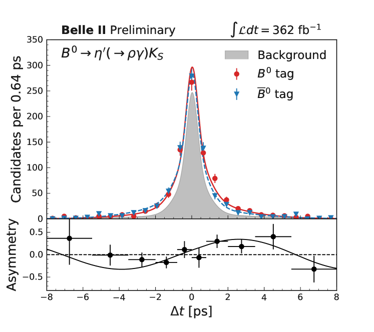
Figure 5: Distribution of $\Delta{t}$ for signal channels separately for $B^{0}$ ($q_{\mathrm{tag}}=+1$) and $\kern 1.79993pt\overline{\kern-1.79993ptB}{}^{0}$ ($q_{\mathrm{tag}}=-1$) tags, for $B^{0}\rightarrow\mathit{{\eta}{}_{\mspace{-3.0mu}\scriptstyle{}}^{\mspace{-1.0mu}\scriptstyle{\prime}}}[\rightarrow\rho\mathit{{\gamma}{}_{\mspace{-3.0mu}\scriptstyle{}}^{\mspace{-1.0mu}\scriptstyle{}}}]K^{0}_{\rm\scriptscriptstyle\textsl{S}}$. The background contribution is also shown as a shaded area. The fit projections corresponding to $B^{0}$ and $\kern 1.79993pt\overline{\kern-1.79993ptB}{}^{0}$ are shown as solid and dashed curves, respectively. The bottom panel shows the asymmetry as defined in Eq. 2, after subtracting the background using the ${{}_{s}Plot}$ technique Pivk and Le Diberder (2005). The horizontal bars represent the widths of the variable-size bins used.

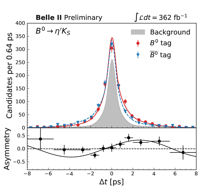
Figure 6: Distribution of $\Delta{t}$ for signal channels separately for $B^{0}$ ($q_{\mathrm{tag}}=+1$) and $\kern 1.79993pt\overline{\kern-1.79993ptB}{}^{0}$ ($q_{\mathrm{tag}}=-1$) tags, combining the two subchannels, $B^{0}\rightarrow\mathit{{\eta}{}_{\mspace{-3.0mu}\scriptstyle{}}^{\mspace{-1.0mu}\scriptstyle{\prime}}}[\rightarrow\eta(\rightarrow\mathit{{\gamma}{}_{\mspace{-3.0mu}\scriptstyle{}}^{\mspace{-1.0mu}\scriptstyle{}}}\mathit{{\gamma}{}_{\mspace{-3.0mu}\scriptstyle{}}^{\mspace{-1.0mu}\scriptstyle{}}})\mathit{{\pi}{}_{\mspace{-3.0mu}\scriptstyle{}}^{\mspace{-1.0mu}\scriptstyle{+}}}\mathit{{\pi}{}_{\mspace{-3.0mu}\scriptstyle{}}^{\mspace{-1.0mu}\scriptstyle{-}}}]K^{0}_{\rm\scriptscriptstyle\textsl{S}}$and $B^{0}\rightarrow\mathit{{\eta}{}_{\mspace{-3.0mu}\scriptstyle{}}^{\mspace{-1.0mu}\scriptstyle{\prime}}}[\rightarrow\rho\mathit{{\gamma}{}_{\mspace{-3.0mu}\scriptstyle{}}^{\mspace{-1.0mu}\scriptstyle{}}}]K^{0}_{\rm\scriptscriptstyle\textsl{S}}$. The background contribution is also shown as a shaded area. The fit projections corresponding to $B^{0}$ and $\kern 1.79993pt\overline{\kern-1.79993ptB}{}^{0}$ are shown as solid and dashed lines, respectively. The bottom panel shows the asymmetry as defined in Eq. 2, after subtracting the background using the ${{}_{s}Plot}$ technique Pivk and Le Diberder (2005). The horizontal bars represent the widths of the variable-size bins used.

The resulting signal yield is $358\pm 20$ for $B^{0}\rightarrow\mathit{{\eta}{}_{\mspace{-3.0mu}\scriptstyle{}}^{\mspace{-1.0mu}\scriptstyle{\prime}}}[\rightarrow\eta(\rightarrow\mathit{{\gamma}{}_{\mspace{-3.0mu}\scriptstyle{}}^{\mspace{-1.0mu}\scriptstyle{}}}\mathit{{\gamma}{}_{\mspace{-3.0mu}\scriptstyle{}}^{\mspace{-1.0mu}\scriptstyle{}}})\mathit{{\pi}{}_{\mspace{-3.0mu}\scriptstyle{}}^{\mspace{-1.0mu}\scriptstyle{+}}}\mathit{{\pi}{}_{\mspace{-3.0mu}\scriptstyle{}}^{\mspace{-1.0mu}\scriptstyle{-}}}]K^{0}_{\rm\scriptscriptstyle\textsl{S}}$, and $471\pm 29$ for $B^{0}\rightarrow\mathit{{\eta}{}_{\mspace{-3.0mu}\scriptstyle{}}^{\mspace{-1.0mu}\scriptstyle{\prime}}}[\rightarrow\rho\mathit{{\gamma}{}_{\mspace{-3.0mu}\scriptstyle{}}^{\mspace{-1.0mu}\scriptstyle{}}}]K^{0}_{\rm\scriptscriptstyle\textsl{S}}$. The purities for the two subchannels are 79% and 30%, respectively. Results for $C\!P$ parameters from a simultaneous fit of the two subchannels are $C_{\mathit{{\eta}{}_{\mspace{-3.0mu}\scriptstyle{}}^{\mspace{-1.0mu}\scriptstyle{\prime}}}\!K^{0}_{\rm\scriptscriptstyle\textsl{S}}}=-0.19\pm 0.08$ and $S_{\mathit{{\eta}{}_{\mspace{-3.0mu}\scriptstyle{}}^{\mspace{-1.0mu}\scriptstyle{\prime}}}\!K^{0}_{\rm\scriptscriptstyle\textsl{S}}}=+0.67\pm 0.10$, where the uncertainties are statistical and obtained from a scan of the likelihood ratio. The results for individual channels are summarized in Table 1. The correlation between $C_{\mathit{{\eta}{}_{\mspace{-3.0mu}\scriptstyle{}}^{\mspace{-1.0mu}\scriptstyle{\prime}}}\!K^{0}_{\rm\scriptscriptstyle\textsl{S}}}$ and $S_{\mathit{{\eta}{}_{\mspace{-3.0mu}\scriptstyle{}}^{\mspace{-1.0mu}\scriptstyle{\prime}}}\!K^{0}_{\rm\scriptscriptstyle\textsl{S}}}$ is $+3.4\%$.

We also explore the subchannel $B^{0}\rightarrow\mathit{{\eta}{}_{\mspace{-3.0mu}\scriptstyle{}}^{\mspace{-1.0mu}\scriptstyle{\prime}}}(\rightarrow\eta\mathit{{\pi}{}_{\mspace{-3.0mu}\scriptstyle{}}^{\mspace{-1.0mu}\scriptstyle{+}}}\mathit{{\pi}{}_{\mspace{-3.0mu}\scriptstyle{}}^{\mspace{-1.0mu}\scriptstyle{-}}})K^{0}_{\rm\scriptscriptstyle\textsl{S}}$ with $\eta$ ($\rightarrow$ $\mathit{{\pi}{}_{\mspace{-3.0mu}\scriptstyle{}}^{\mspace{-1.0mu}\scriptstyle{+}}}$ $\mathit{{\pi}{}_{\mspace{-3.0mu}\scriptstyle{}}^{\mspace{-1.0mu}\scriptstyle{-}}}$ $\pi^{0}$). We reconstruct this final state combining four charged pions, selected using the same criteria for the second subchannel, and one neutral pion decaying to a pair of photons, with an invariant mass $0.120<m(\gamma\gamma)<0.145{\mathrm{\,Ge\kern-1.00006ptV\!/}c^{2}}$. We require $E_{\gamma}>80\mathrm{\,Me\kern-1.00006ptV}$ for photons detected in the forward region, $30\mathrm{\,Me\kern-1.00006ptV}$ for the barrel region, and $60\mathrm{\,Me\kern-1.00006ptV}$ for the backward region, to account for the different levels of background in the three ECL regions. The selection on $E_{\gamma}$ are looser than for the other subchannels to improve efficiency. The $\eta$ candidate is required to have an invariant mass in the range $0.52<m(\pi^{+}\pi^{-}\pi^{0})<0.57{\mathrm{\,Ge\kern-1.00006ptV\!/}c^{2}}$ while the mass difference $\Delta{m}$ between $\eta^{\prime}$ and $\eta$ candidates must satisfy $0.40<\Delta m<0.42{\mathrm{\,Ge\kern-1.00006ptV\!/}c^{2}}$. The other selection criteria for the $K^{0}_{\rm\scriptscriptstyle\textsl{S}}$ and $B^{0}$ candidates are the same as for the other subchannels. The signal yield is $55\pm 8$, and the purity is 55%. We perform the vertex fit and determine the resolution model, whose functional form is similar to that used in Ref. Tajima et al. (2004). The measured $C\!P$ asymmetries, $C_{\eta^{\prime}(3\pi)K^{0}_{\rm\scriptscriptstyle\textsl{S}}}=0.11^{+0.32}_{-0.31}$ and $S_{\eta^{\prime}(3\pi)K^{0}_{\rm\scriptscriptstyle\textsl{S}}}=0.25^{+0.47}_{-0.53}$ (the uncertainties are statistical) are consistent with those determined in the other two subchannels, but significantly less precise. Figure 7 shows the results of the $C\!P$ asymmetry fit on the $B^{0}\rightarrow\eta^{\prime}[\rightarrow\eta(\rightarrow\pi^{+}\pi^{-}\pi^{0})\pi^{+}\pi^{-}]K^{0}_{\rm\scriptscriptstyle\textsl{S}}$ subchannel. The results of this subchannel are not used for final results since their statistical significance is negligible.

Table 1: Summary of results on $C_{\mathit{{\eta}{}_{\mspace{-3.0mu}\scriptstyle{}}^{\mspace{-1.0mu}\scriptstyle{\prime}}}\!K^{0}_{\rm\scriptscriptstyle\textsl{S}}}$ and $S_{\mathit{{\eta}{}_{\mspace{-3.0mu}\scriptstyle{}}^{\mspace{-1.0mu}\scriptstyle{\prime}}}\!K^{0}_{\rm\scriptscriptstyle\textsl{S}}}$ for the three subchannels, identified by the $\mathit{{\eta}{}_{\mspace{-3.0mu}\scriptstyle{}}^{\mspace{-1.0mu}\scriptstyle{\prime}}}$ decay. The last subchannel is not included in the simultaneous fit. The uncertainties are statistical only.

Channel	Signal yield	$C_{\mathit{{\eta}{}_{\mspace{-3.0mu}\scriptstyle{}}^{\mspace{-1.0mu}\scriptstyle{\prime}}}\!K^{0}_{\rm\scriptscriptstyle\textsl{S}}}$	$S_{\mathit{{\eta}{}_{\mspace{-3.0mu}\scriptstyle{}}^{\mspace{-1.0mu}\scriptstyle{\prime}}}\!K^{0}_{\rm\scriptscriptstyle\textsl{S}}}$
$\mathit{{\eta}{}_{\mspace{-3.0mu}\scriptstyle{}}^{\mspace{-1.0mu}\scriptstyle{\prime}}}\rightarrow\eta_{\mathit{{\gamma}{}_{\mspace{-3.0mu}\scriptstyle{}}^{\mspace{-1.0mu}\scriptstyle{}}}\mathit{{\gamma}{}_{\mspace{-3.0mu}\scriptstyle{}}^{\mspace{-1.0mu}\scriptstyle{}}}}\mathit{{\pi}{}_{\mspace{-3.0mu}\scriptstyle{}}^{\mspace{-1.0mu}\scriptstyle{+}}}\mathit{{\pi}{}_{\mspace{-3.0mu}\scriptstyle{}}^{\mspace{-1.0mu}\scriptstyle{-}}}$	$358\pm 20$	$-0.10\pm 0.13$	$0.69\pm 0.14$
$\mathit{{\eta}{}_{\mspace{-3.0mu}\scriptstyle{}}^{\mspace{-1.0mu}\scriptstyle{\prime}}}\rightarrow\rho\mathit{{\gamma}{}_{\mspace{-3.0mu}\scriptstyle{}}^{\mspace{-1.0mu}\scriptstyle{}}}$	$471\pm 29$	$-0.24\pm 0.10$	$0.65\pm 0.13$
$\mathit{{\eta}{}_{\mspace{-3.0mu}\scriptstyle{}}^{\mspace{-1.0mu}\scriptstyle{\prime}}}\rightarrow\eta_{3\mathit{{\pi}{}_{\mspace{-3.0mu}\scriptstyle{}}^{\mspace{-1.0mu}\scriptstyle{}}}}\mathit{{\pi}{}_{\mspace{-3.0mu}\scriptstyle{}}^{\mspace{-1.0mu}\scriptstyle{+}}}\mathit{{\pi}{}_{\mspace{-3.0mu}\scriptstyle{}}^{\mspace{-1.0mu}\scriptstyle{-}}}$	$55\pm 8\leavevmode\nobreak\ \,$	$\leavevmode\nobreak\ \,\,0.11\pm 0.32$	$0.25\pm 0.50$
Sim. fit	$829\pm 35$	$-0.19\pm 0.08$	$0.67\pm 0.10$

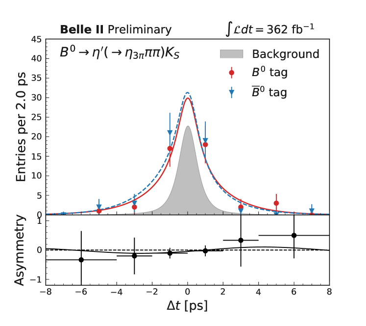
Figure 7: Distribution of $\Delta{t}$ for the $B^{0}\rightarrow\eta^{\prime}[\rightarrow\eta(\rightarrow\pi^{+}\pi^{-}\pi^{0})\pi^{+}\pi^{-}]K^{0}_{\rm\scriptscriptstyle\textsl{S}}$ channel, separately for $B^{0}$ ($q_{\mathrm{tag}}=+1$) and $B^{0}$ ($q_{\mathrm{tag}}=-1$) tagged events. The fit projections corresponding to $B^{0}$ and $\kern 1.79993pt\overline{\kern-1.79993ptB}{}^{0}$ are shown as solid and dashed lines, respectively. The background is also shown as a shaded area. The bottom panel shows the asymmetry as defined in Eq. 2, using the ${{}_{s}Plot}$ technique Pivk and Le Diberder (2005) to subtract the background. The horizontal bars represent the widths of the variable size bins used.

V Systematic uncertainties

We consider several sources of possible systematic uncertainties, which are listed in Table 2.

Table 2: Summary of systematic uncertainties for $C_{\mathit{{\eta}{}_{\mspace{-3.0mu}\scriptstyle{}}^{\mspace{-1.0mu}\scriptstyle{\prime}}}\!K^{0}_{\rm\scriptscriptstyle\textsl{S}}}$ and $S_{\mathit{{\eta}{}_{\mspace{-3.0mu}\scriptstyle{}}^{\mspace{-1.0mu}\scriptstyle{\prime}}}\!K^{0}_{\rm\scriptscriptstyle\textsl{S}}}$.

Source	$C_{\mathit{{\eta}{}_{\mspace{-3.0mu}\scriptstyle{}}^{\mspace{-1.0mu}\scriptstyle{\prime}}}\!K^{0}_{\rm\scriptscriptstyle\textsl{S}}}$	$S_{\mathit{{\eta}{}_{\mspace{-3.0mu}\scriptstyle{}}^{\mspace{-1.0mu}\scriptstyle{\prime}}}\!K^{0}_{\rm\scriptscriptstyle\textsl{S}}}$
Signal and continuum yields	$<0.001$	0.002
SxF and $B\!\kern 1.79993pt\overline{\kern-1.79993ptB}{}$ yields	$<0.001$	0.006
$C_{\rm BDT}$ mismodeling	0.004	0.010
Signal and background modeling	0.020	0.014
Observable correlations	0.008	0.001
$\Delta{t}$ resolution fixed parameters	0.005	0.009
$\Delta{t}$ resolution model	0.004	0.019
Flavor tagging	0.007	0.004
$\tau_{B^{0}}$ and $\Delta{m_{d}}$	$<0.001$	0.002
Fit bias	0.003	0.002
Tracker misalignment	0.004	0.006
Momentum scale	0.001	0.001
Beam spot	0.002	0.002
$B$-meson motion in the $\Upsilon(4\mathrm{S})$ frame	$<0.001$	0.017
Tag-side interference	0.005	0.011
$B\!\kern 1.79993pt\overline{\kern-1.79993ptB}{}$ background asymmetry	0.008	0.006
Candidate selection	0.007	0.009
Total	0.027	0.037

To determine most of the systematic uncertainties, we use ensembles of simulated samples. For signal and SxF events we use sampling with replacement Efron (1979) from the available simulated samples, while continuum and $B\!\kern 1.79993pt\overline{\kern-1.79993ptB}{}$ backgrounds are sampled from the PDF used for modeling, due to the limited size of simulated samples.

To evaluate the impact of the uncertainties of signal and continuum yields in the second fit step, we vary them individually by assuming alternate values, corresponding to $\pm 1$-standard-deviation fluctuations of the first fit results. We then consider the difference between the values of $C_{\mathit{{\eta}{}_{\mspace{-3.0mu}\scriptstyle{}}^{\mspace{-1.0mu}\scriptstyle{\prime}}}\!K^{0}_{\rm\scriptscriptstyle\textsl{S}}}$ and $S_{\mathit{{\eta}{}_{\mspace{-3.0mu}\scriptstyle{}}^{\mspace{-1.0mu}\scriptstyle{\prime}}}\!K^{0}_{\rm\scriptscriptstyle\textsl{S}}}$ from the nominal results as a systematic uncertainty.

The SxF and $B\!\kern 1.79993pt\overline{\kern-1.79993ptB}{}$ yields are fixed to their values obtained in simulation. To estimate the systematic uncertainties, we let the fit determine the $B\!\kern 1.79993pt\overline{\kern-1.79993ptB}{}$ yield for all $r$ bins, one at a time to ensure the fit convergence. The average ratio between the fit result and expectation is $0.9\pm 0.2$, and the average uncertainty of $B\!\kern 1.79993pt\overline{\kern-1.79993ptB}{}$ yield in each bin is about $50\%$. We vary the $B\!\kern 1.79993pt\overline{\kern-1.79993ptB}{}$ yield by this uncertainty and take the variations in the $C\!P$ asymmetry parameters as a systematic uncertainty. We also vary the SxF yield by the same uncertainty (50%), and evaluate the variations on $C\!P$ asymmetry parameters.

The impact of any $C_{\rm BDT}$ mismodeling is evaluated by comparing the results obtained using the data sidebands for its training with those in which the training is performed on continuum simulated events.

Similarly to what is done for yields, the parameters of PDF shapes used to model the various components are varied within their statistical uncertainties if they are determined in the first step of the fit. This is the case for the signal and continuum components. The variations of $C_{\mathit{{\eta}{}_{\mspace{-3.0mu}\scriptstyle{}}^{\mspace{-1.0mu}\scriptstyle{\prime}}}\!K^{0}_{\rm\scriptscriptstyle\textsl{S}}}$ and $S_{\mathit{{\eta}{}_{\mspace{-3.0mu}\scriptstyle{}}^{\mspace{-1.0mu}\scriptstyle{\prime}}}\!K^{0}_{\rm\scriptscriptstyle\textsl{S}}}$ due to alternative values of each parameter are summed linearly, to account for possible correlation, and used as a systematic uncertainty. The parameters fixed from simulation are allowed to vary, individually, in the $C\!P$ asymmetry fit. We take the difference of $C_{\mathit{{\eta}{}_{\mspace{-3.0mu}\scriptstyle{}}^{\mspace{-1.0mu}\scriptstyle{\prime}}}\!K^{0}_{\rm\scriptscriptstyle\textsl{S}}}$ and $S_{\mathit{{\eta}{}_{\mspace{-3.0mu}\scriptstyle{}}^{\mspace{-1.0mu}\scriptstyle{\prime}}}\!K^{0}_{\rm\scriptscriptstyle\textsl{S}}}$ from the nominal results as a systematic uncertainty, summing the differences in quadrature.

The impact of the correlation between the fit observables, mostly between $M_{\text{bc}}$ and $\Delta{E}$, is estimated using ensembles of signal events simulated with correlation, sampled with replacement from the available simulated samples, and without correlation, by sampling the PDFs, and comparing the two sets of results.

The systematic uncertainty due to the $\Delta{t}$ resolution model is estimated by repeating the fit under alternative assumptions for values of the resolution parameters within the uncertainties obtained from the fit on the $B\rightarrow D^{(*)-}\mathit{{\pi}{}_{\mspace{-3.0mu}\scriptstyle{}}^{\mspace{-1.0mu}\scriptstyle{+}}}$ control sample. We also compare the result of a fit using the resolution parameters obtained by fitting the simulated $B\rightarrow\mathit{{\eta}{}_{\mspace{-3.0mu}\scriptstyle{}}^{\mspace{-1.0mu}\scriptstyle{\prime}}}K^{0}_{\rm\scriptscriptstyle\textsl{S}}$ signal events with the nominal fit, and take the difference on $C_{\mathit{{\eta}{}_{\mspace{-3.0mu}\scriptstyle{}}^{\mspace{-1.0mu}\scriptstyle{\prime}}}\!K^{0}_{\rm\scriptscriptstyle\textsl{S}}}$ and $S_{\mathit{{\eta}{}_{\mspace{-3.0mu}\scriptstyle{}}^{\mspace{-1.0mu}\scriptstyle{\prime}}}\!K^{0}_{\rm\scriptscriptstyle\textsl{S}}}$ as a systematic uncertainty.

The flavor-tagging parameters are varied within their statistical uncertainties. The same is done for the physics parameters $\tau_{B^{0}}$ and $\Delta{m_{d}}$, using the uncertainties on their world-average values. Small fit biases found on $C_{\mathit{{\eta}{}_{\mspace{-3.0mu}\scriptstyle{}}^{\mspace{-1.0mu}\scriptstyle{\prime}}}\!K^{0}_{\rm\scriptscriptstyle\textsl{S}}}$ and $S_{\mathit{{\eta}{}_{\mspace{-3.0mu}\scriptstyle{}}^{\mspace{-1.0mu}\scriptstyle{\prime}}}\!K^{0}_{\rm\scriptscriptstyle\textsl{S}}}$ by fits to large simulated samples are also included.

The impact of tracker misalignment is estimated with dedicated simulation samples with four different misalignment scenarios. The effects on charged-particle momentum scale due to imperfect modeling of the magnetic field, and the uncertainty on the beam spot determination, were studied in a previous analysis that used similar reconstruction strategies Adachi et al. (2023).

We estimate the effect of neglecting the small motion of the $B$ meson in the $\Upsilon(4\mathrm{S})$ rest frame by calculating $\Delta{t}$ from simulated signal events and comparing the true $\Delta{t}$ with that based on true $\Delta{z}$.

The $\Delta{t}$ model in Eq. 2 assumes that the ${B}_{\text{tag}}$ decays into a flavor-specific mode. The impact of tag-side interference, namely the presence of Cabibbo-suppressed $b\rightarrow{u\bar{c}s}$ decays in the ${B}_{\text{tag}}$ with different weak phase Long et al. (2003), is estimated by correcting for the observed asymmetry using previous measurements Amhis et al. (2023). We conservatively assume that all events are tagged by hadronic $B$ decays, where the effect is largest. We use the difference with respect to the nominal asymmetry as a systematic uncertainty.

The $B\!\kern 1.79993pt\overline{\kern-1.79993ptB}{}$ background is small and dominated by $b\rightarrow{c}$ decays. The possible presence of $C\!P$ violation in the $B\!\kern 1.79993pt\overline{\kern-1.79993ptB}{}$ background is estimated conservatively by assuming that all this background has a $C\!P$ asymmetry with $(C_{C\!P},S_{C\!P})=(\pm 0.2,0)$ or $(0,\pm 0.2)$ and taking the largest variation on $C_{\mathit{{\eta}{}_{\mspace{-3.0mu}\scriptstyle{}}^{\mspace{-1.0mu}\scriptstyle{\prime}}}\!K^{0}_{\rm\scriptscriptstyle\textsl{S}}}$ and $S_{\mathit{{\eta}{}_{\mspace{-3.0mu}\scriptstyle{}}^{\mspace{-1.0mu}\scriptstyle{\prime}}}\!K^{0}_{\rm\scriptscriptstyle\textsl{S}}}$ as a systematic uncertainty.

Finally, the impact of the candidate selection is evaluated by repeating the full analysis with all multiple candidates and comparing with the results obtained using only the one with best vertex-$\chi^{2}$.

VI Summary

A measurement of $C\!P$ asymmetries in $B\rightarrow\mathit{{\eta}{}_{\mspace{-3.0mu}\scriptstyle{}}^{\mspace{-1.0mu}\scriptstyle{\prime}}}K^{0}_{\rm\scriptscriptstyle\textsl{S}}$ decays is conducted using $e^{+}e^{-}$ collision data collected in 2019–-2022 by the Belle II experiment at the SuperKEKB collider. We find $829\pm 35$ signal decays in a sample of $(387\pm 6)\text{\times}{10}^{6}$ $B\!\kern 1.79993pt\overline{\kern-1.79993ptB}{}$ events and measure the $C\!P$ asymmetries to be

$$\begin{split}C_{\mathit{{\eta}{}_{\mspace{-3.0mu}\scriptstyle{}}^{\mspace{-1.0mu}\scriptstyle{\prime}}}\!K^{0}_{\rm\scriptscriptstyle\textsl{S}}}&=-0.19\pm 0.08\pm 0.03,\\ S_{\mathit{{\eta}{}_{\mspace{-3.0mu}\scriptstyle{}}^{\mspace{-1.0mu}\scriptstyle{\prime}}}\!K^{0}_{\rm\scriptscriptstyle\textsl{S}}}&=+0.67\pm 0.10\pm 0.04,\\ \end{split}$$ (5)

where the first uncertainties are statistical and the second systematic. This measurement is based on the subchannels $B^{0}\rightarrow\mathit{{\eta}{}_{\mspace{-3.0mu}\scriptstyle{}}^{\mspace{-1.0mu}\scriptstyle{\prime}}}[\rightarrow\eta(\rightarrow\mathit{{\gamma}{}_{\mspace{-3.0mu}\scriptstyle{}}^{\mspace{-1.0mu}\scriptstyle{}}}\mathit{{\gamma}{}_{\mspace{-3.0mu}\scriptstyle{}}^{\mspace{-1.0mu}\scriptstyle{}}})\mathit{{\pi}{}_{\mspace{-3.0mu}\scriptstyle{}}^{\mspace{-1.0mu}\scriptstyle{+}}}\mathit{{\pi}{}_{\mspace{-3.0mu}\scriptstyle{}}^{\mspace{-1.0mu}\scriptstyle{-}}}]K^{0}_{\rm\scriptscriptstyle\textsl{S}}$and $B^{0}\rightarrow\mathit{{\eta}{}_{\mspace{-3.0mu}\scriptstyle{}}^{\mspace{-1.0mu}\scriptstyle{\prime}}}[\rightarrow\rho\mathit{{\gamma}{}_{\mspace{-3.0mu}\scriptstyle{}}^{\mspace{-1.0mu}\scriptstyle{}}}]K^{0}_{\rm\scriptscriptstyle\textsl{S}}$.

This is the first measurement of $C\!P$ violation in this channel at Belle II. The results are in agreement with the current world averages, and have sensitivities close to those of Belle Šantelj et al. (2014) and BaBar Aubert et al. (2009b), despite the smaller data size.

VII Acknowledgements

This work, based on data collected using the Belle II detector, which was built and commissioned prior to March 2019, was supported by Higher Education and Science Committee of the Republic of Armenia Grant No. 23LCG-1C011; Australian Research Council and Research Grants No. DP200101792, No. DP210101900, No. DP210102831, No. DE220100462, No. LE210100098, and No. LE230100085; Austrian Federal Ministry of Education, Science and Research, Austrian Science Fund No. P 31361-N36 and No. J4625-N, and Horizon 2020 ERC Starting Grant No. 947006 “InterLeptons”; Natural Sciences and Engineering Research Council of Canada, Compute Canada and CANARIE; National Key R&D Program of China under Contract No. 2022YFA1601903, National Natural Science Foundation of China and Research Grants No. 11575017, No. 11761141009, No. 11705209, No. 11975076, No. 12135005, No. 12150004, No. 12161141008, and No. 12175041, and Shandong Provincial Natural Science Foundation Project ZR2022JQ02; the Czech Science Foundation Grant No. 22-18469S; European Research Council, Seventh Framework PIEF-GA-2013-622527, Horizon 2020 ERC-Advanced Grants No. 267104 and No. 884719, Horizon 2020 ERC-Consolidator Grant No. 819127, Horizon 2020 Marie Sklodowska-Curie Grant Agreement No. 700525 “NIOBE” and No. 101026516, and Horizon 2020 Marie Sklodowska-Curie RISE project JENNIFER2 Grant Agreement No. 822070 (European grants); L’Institut National de Physique Nucléaire et de Physique des Particules (IN2P3) du CNRS and L’Agence Nationale de la Recherche (ANR) under grant ANR-21-CE31-0009 (France); BMBF, DFG, HGF, MPG, and AvH Foundation (Germany); Department of Atomic Energy under Project Identification No. RTI 4002, Department of Science and Technology, and UPES SEED funding programs No. UPES/R&D-SEED-INFRA/17052023/01 and No. UPES/R&D-SOE/20062022/06 (India); Israel Science Foundation Grant No. 2476/17, U.S.-Israel Binational Science Foundation Grant No. 2016113, and Israel Ministry of Science Grant No. 3-16543; Istituto Nazionale di Fisica Nucleare and the Research Grants BELLE2; Japan Society for the Promotion of Science, Grant-in-Aid for Scientific Research Grants No. 16H03968, No. 16H03993, No. 16H06492, No. 16K05323, No. 17H01133, No. 17H05405, No. 18K03621, No. 18H03710, No. 18H05226, No. 19H00682, No. 20H05850, No. 20H05858, No. 22H00144, No. 22K14056, No. 22K21347, No. 23H05433, No. 26220706, and No. 26400255, the National Institute of Informatics, and Science Information NETwork 5 (SINET5), and the Ministry of Education, Culture, Sports, Science, and Technology (MEXT) of Japan; National Research Foundation (NRF) of Korea Grants No. 2016R1D1A1B02012900, No. 2018R1A2B3003643, No. 2018R1A6A1A06024970, No. 2019R1I1A3A01058933, No. 2021R1A6A1A03043957, No. 2021R1F1A1060423, No. 2021R1F1A1064008, No. 2022R1A2C1003993, and No. RS-2022-00197659, Radiation Science Research Institute, Foreign Large-Size Research Facility Application Supporting project, the Global Science Experimental Data Hub Center of the Korea Institute of Science and Technology Information and KREONET/GLORIAD; Universiti Malaya RU grant, Akademi Sains Malaysia, and Ministry of Education Malaysia; Frontiers of Science Program Contracts No. FOINS-296, No. CB-221329, No. CB-236394, No. CB-254409, and No. CB-180023, and SEP-CINVESTAV Research Grant No. 237 (Mexico); the Polish Ministry of Science and Higher Education and the National Science Center; the Ministry of Science and Higher Education of the Russian Federation and the HSE University Basic Research Program, Moscow; University of Tabuk Research Grants No. S-0256-1438 and No. S-0280-1439 (Saudi Arabia); Slovenian Research Agency and Research Grants No. J1-9124 and No. P1-0135; Agencia Estatal de Investigacion, Spain Grant No. RYC2020-029875-I and Generalitat Valenciana, Spain Grant No. CIDEGENT/2018/020; National Science and Technology Council, and Ministry of Education (Taiwan); Thailand Center of Excellence in Physics; TUBITAK ULAKBIM (Turkey); National Research Foundation of Ukraine, Project No. 2020.02/0257, and Ministry of Education and Science of Ukraine; the U.S. National Science Foundation and Research Grants No. PHY-1913789 and No. PHY-2111604, and the U.S. Department of Energy and Research Awards No. DE-AC06-76RLO1830, No. DE-SC0007983, No. DE-SC0009824, No. DE-SC0009973, No. DE-SC0010007, No. DE-SC0010073, No. DE-SC0010118, No. DE-SC0010504, No. DE-SC0011784, No. DE-SC0012704, No. DE-SC0019230, No. DE-SC0021274, No. DE-SC0021616, No. DE-SC0022350, No. DE-SC0023470; and the Vietnam Academy of Science and Technology (VAST) under Grants No. NVCC.05.12/22-23 and No. DL0000.02/24-25.

These acknowledgements are not to be interpreted as an endorsement of any statement made by any of our institutes, funding agencies, governments, or their representatives.

We thank the SuperKEKB team for delivering high-luminosity collisions; the KEK cryogenics group for the efficient operation of the detector solenoid magnet; the KEK computer group and the NII for on-site computing support and SINET6 network support; and the raw-data centers at BNL, DESY, GridKa, IN2P3, INFN, and the University of Victoria for off-site computing support.

References

- Cabibbo (1963) N. Cabibbo, Phys. Rev. Lett. 10, 531 (1963).
- Kobayashi and Maskawa (1973) M. Kobayashi and T. Maskawa, Prog. Theor. Phys. 49, 652 (1973).
- Adachi et al. (2012) I. Adachi et al. (Belle Collaboration), Phys. Rev. Lett. 108, 171802 (2012).
- Aubert et al. (2009a) B. Aubert et al. (BaBar Collaboration), Phys. Rev. D 79, 072009 (2009a).
- Aaij et al. (2015) R. Aaij et al. (LHCb Collaboration), Phys. Rev. Lett. 115, 031601 (2015).
- Altmannshofer et al. (2019) W. Altmannshofer et al., PTEP 2019, 123C01 (2019), arXiv:1808.10567 [hep-ex] .
- Ed. A. J. Bevan, B. Golob, Th. Mannel, S. Prell, and B. D. Yabsley (2014) Ed. A. J. Bevan, B. Golob, Th. Mannel, S. Prell, and B. D. Yabsley, Eur. Phys. J. C74, 3026 (2014), arXiv:1406.6311 [hep-ex] .
- Beneke (2005) M. Beneke, Phys. Lett. B 620, 143 (2005), arXiv:hep-ph/0505075 .
- (9) See, e.g., A. Ceccucci, Z. Ligeti and Y. Sakai, Sec.12 in Ref. Workman et al. (2022).
- Šantelj et al. (2014) L. Šantelj et al. (Belle Collaboration), J. High Energy Phys 10, 165 (2014), arXiv:1408.5991 [hep-ex] .
- Aubert et al. (2009b) B. Aubert et al. (BaBar Collaboration), Phys. Rev. D 79, 052003 (2009b), arXiv:0809.1174 [hep-ex] .
- Amhis et al. (2023) Y. S. Amhis et al. (Heavy Flavor Averaging Group), Phys. Rev. D 107, 052008 (2023), arXiv:2206.07501 [hep-ex] .
- Akai, Furukawa, and Koiso (2018) K. Akai, K. Furukawa, and H. Koiso, Nucl. Instrum. Meth. A907, 188 (2018), arXiv:1809.01958 [physics.acc-ph] .
- Abudinén et al. (2022) F. Abudinén et al. (Belle II Collaboration), Eur. Phys. J. C 82 (2022), 10.1140/epjc/s10052-022-10180-9.
- Abe et al. (2010) T. Abe et al. (Belle II Collaboration), (2010), arXiv:1011.0352 [physics.ins-det] .
- Jadach, Ward, and Wa̧s (2000) S. Jadach, B. F. L. Ward, and Z. Wa̧s, Comput. Phys. Commun. 130, 260 (2000), arXiv:hep-ph/9912214 [hep-ph] .
- Sjöstrand et al. (2015) T. Sjöstrand et al., Comput. Phys. Commun. 191, 159 (2015), arXiv:1410.3012 [hep-ph] .
- Lange (2001) D. J. Lange, Proceedings, 7th International Conference on physics at hadron machines (BEAUTY 2000): Maagan, Israel, September 13-18, 2000, Nucl. Instrum. Meth. A462, 152 (2001).
- Agostinelli et al. (2003) S. Agostinelli et al. (GEANT4 Collaboration), Nucl.Instrum.Meth. A506, 250 (2003).
- Kuhr et al. (2019) T. Kuhr et al. (Belle II Framework Software Group), Comput. Softw. Big Sci. 3, 1 (2019), arXiv:1809.04299 [physics.comp-ph] .
- Belle II Collaboration (2022) Belle II Collaboration, “Belle II Analysis Software Framework (basf2),” (2022).
- Bertacchi et al. (2021) V. Bertacchi et al. (Belle II Tracking Group), Comput. Phys. Commun. 259, 107610 (2021), arXiv:2003.12466 [physics.ins-det] .
- Krohn et al. (2020) J.-F. Krohn et al. (Belle II Analysis Software Group), Nucl. Instrum. Meth. A976, 164269 (2020), arXiv:1901.11198 [hep-ex] .
- Hulsbergen (2005) W. D. Hulsbergen, Nucl. Instrum. Meth. 552, 566 (2005).
- Workman et al. (2022) R. L. Workman et al. (Particle Data Group), PTEP 2022, 083C01 (2022).
- Waltenberger (2011) W. Waltenberger, IEEE Trans. Nucl. Sci. 58, 434 (2011).
- Dey and Soffer (2020) S. Dey and A. Soffer, Springer Proc. Phys. 248, 411 (2020).
- Keck (2017) T. Keck, Comput. Softw. Big Sci. 1, 2 (2017).
- Brandt et al. (1964) S. Brandt et al., Phys. Lett. 12, 57 (1964).
- Fox and Wolfram (1978) G. C. Fox and S. Wolfram, Phys. Rev. Lett. 41, 1581 (1978).
- Lee et al. (2003) S. H. Lee et al. (Belle Collaboration), Phys. Rev. Lett. 91, 261801 (2003).
- Asner et al. (1996) D. M. Asner et al. (CLEO Collaboration), Phys. Rev. D 53, 1039 (1996).
- Gaiser (1982) J. Gaiser, Charmonium spectroscopy from radiative decays of the and , Ph.D. thesis, Stanford University (1982).
- Skwarnicki (1986) T. Skwarnicki, A study of the radiative CASCADE transitions between the Upsilon-Prime and Upsilon resonances, Ph.D. thesis, Cracow, INP (1986).
- Oreglia et al. (1982) M. Oreglia, E. Bloom, F. Bulos, R. Chestnut, J. Gaiser, G. Godfrey, C. Kiesling, W. Lockman, D. L. Scharre, R. Partridge, C. Peck, F. C. Porter, D. Antreasyan, Y.-F. Gu, W. Kollmann, M. Richardson, K. Strauch, K. Wacker, D. Aschman, T. Burnett, C. Newman, M. Cavalli-Sforza, D. Coyne, H. Sadrozinski, R. Hofstadter, I. Kirkbride, H. Kolanoski, K. Königsmann, A. Liberman, J. O’Reilly, B. Pollock, and J. Tompkins, Phys. Rev. D 25, 2259 (1982).
- Albrecht et al. (1990) H. Albrecht et al. (ARGUS Collaboration), Phys. Lett. B 241, 278 (1990).
- Abudinén et al. (2023) F. Abudinén et al. (Belle II Collaboration), Phys. Rev. D 107, L091102 (2023).
- Pivk and Le Diberder (2005) M. Pivk and F. R. Le Diberder, Nucl. Instrum. Meth. A555, 356 (2005), arXiv:physics/0402083 [physics.data-an] .
- Tajima et al. (2004) H. Tajima et al., Nucl. Instrum. Meth. 533, 370 (2004).
- Efron (1979) B. Efron, The Annals of Statistics 7, 1 (1979).
- Adachi et al. (2023) I. Adachi et al. (Belle Collaboration), (2023), arXiv:2302.12898 [hep-ex] .
- Long et al. (2003) O. Long et al., Phys. Rev. D 68, 034010 (2003).