sm.pdf

Evidence that the AT transition disappears below six dimensions

Abstract

One of the key predictions of Parisi’s broken replica symmetry theory of spin glasses is the existence of a phase transition in an applied field to a state with broken replica symmetry. This transition takes place at the de Almeida-Thouless (AT) line in the $h-T$ plane. We have studied this line in the power-law diluted Heisenberg spin glass in which the probability that two spins separated by a distance $r$ interact with each other falls as $1/r^{2\sigma}$. In the presence of a random vector-field of variance $h_{r}^{2}$ the phase transition is in the universality class of the Ising spin glass in a field. Tuning $\sigma$ is equivalent to changing the dimension $d$ of the short-range system, with the relation being $d=2/(2\sigma-1)$ for $\sigma<2/3$. We have found by numerical simulations that $h_{\text{AT}}^{2}\sim(2/3-\sigma)$ implying that the AT line does not exist below $6$ dimensions and that the Parisi scheme is not appropriate for spin glasses in three dimensions.

The relevance of the replica symmetry breaking (RSB) scheme of Parisi (Parisi, 1979; Mézard et al., 1986) for physical spin glasses in three dimensions has occasioned doubts from its earliest days (Bray and Roberts, 1980). These doubts have mostly arisen from studies of the de Almeida-Thouless (AT) line (de Almeida and Thouless, 1978). This is the line in the field $h$ and temperature $T$ plane where the replica symmetric high-temperature phase changes to a phase with broken replica symmetry (see Fig. 1). The Parisi scheme has now been rigorously proved to solve the Sherrington-Kirkpatrick (SK) mean-field model (Sherrington and Kirkpatrick, 1975), in which all spins interact with each other. In that model in the presence of a field $h$, the AT line $h_{\text{AT}}(T)$ for temperatures $T$ close to $T_{c}$, the zero-field transition temperature, takes the form

$$\left(\frac{h_{\text{AT}}(T)}{T_{c}}\right)^{2}=A(d)\left(1-\frac{T}{T_{c}}\right)^{\zeta}.$$ (1)

The exponent $\zeta=3$ in the SK model and remains at 3 for all $d>8$. It takes the value $d/2-1$ when $8>d>6$ (Green et al., 1983; Fisher and Sompolinsky, 1985). For $d<6$, should the AT line then still exist, $\zeta=\gamma+\beta$, where the exponent $\gamma$ describes the divergence of the zero-field spin glass susceptibility $\chi_{\text{SG}}$ as $T\to T_{c}$, and $\beta$ describes how the Edwards-Anderson order parameter $q_{\text{EA}}$ goes to zero in the same limit Fisher and Sompolinsky (1985). Both these zero-field exponents have an expansion in powers of $\epsilon$ where $d=6-\epsilon$ (Harris et al., 1976). Back in 1980 Bray and Roberts (Bray and Roberts, 1980) were unable to find a fixed point for the exponents at the AT line. One possibility which they suggested as an explanation was that for $d<6$ there simply was no AT line. However, the possibility that there was a non-perturbative fixed point could not be ruled out (but if such exists, it still remains to be discovered).

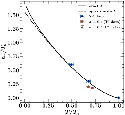
Figure 1: The AT line. The solid line is the exact AT line for the SK model, calculated as in Ref. Sharma and Young (2010). The dashed line is the approximation to it of Eq. (1) with $\zeta=3$. Marked on the diagram by filled circles are the results of the simulations on the SK model in Ref. Sharma and Young (2010). The red square point, derived from varying the temperature $T$ at fixed $h_{r}$, and the upwards arrow point, derived from varying the field at fixed temperature, are the result of our simulations at $\sigma=0.6$, which despite corresponding to 10 dimensions, have values of $h_{\text{AT}}$ suppressed by fluctuations from those which would be estimated from the SK model when only adjusting the zero-field transition temperature $T_{c}$.

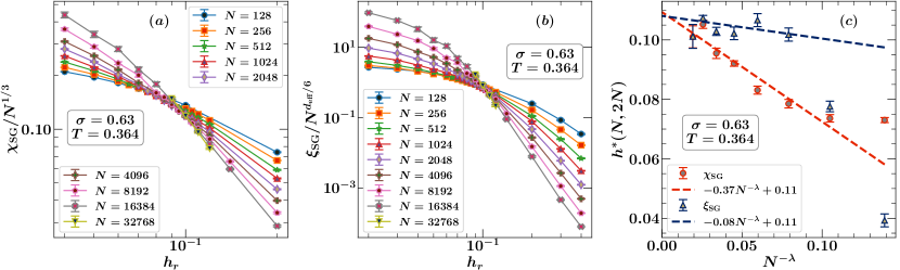
Figure 2: Finite size scaling analyses of $\chi_{\text{SG}}$ data (figure (a)), and $\xi_{\text{SG}}$ data (figure (b)), for $\sigma=0.630$ obtained by fixing the temperature to $T=0.364\,(=0.675\,T_{c})$ and varying the field. Both the plots show that the curves for different system sizes intersect. Figure (c) shows the data for the intersection fields $h^{*}(N,2N)$ between pairs of adjacent system sizes, plotted as a function of $N^{-\lambda}$. Using $\lambda=0.407$ we fitted the $h^{*}(N,2N)$ data linearly with Eq. (14) and the values of the transition field so obtained are $h_{\text{AT}}(T=0.364)=0.1094\pm 0.0012$ from $\chi_{\text{SG}}$ and $h_{\text{AT}}(T=0.364)=0.1081\pm 0.0015$ from $\xi_{\text{SG}}$ (see Table S2 in the supplementary material for details).

Another argument suggested long ago was that of Moore and Bray (Moore and Bray, 1985). In $d<6$ the dependence on $\gamma$ and $\beta$ of the form of the AT line as $\zeta=\gamma+\beta$ indicates that the applied field $h$ has the scaling dimension of the ordering field of the spin glass. For $d>6$ that is not the case, as then $\gamma+\beta=2$ for all $d>6$. Usually when the ordering field is present there is no phase transition. For example, for a ferromagnet in its ordering field (which is a uniform field) there is no phase transition as the temperature is lowered. A phase transition only occurs for vanishing field. The suggestion of Moore and Bray was that because the applied field had the scaling dimensions of the ordering field in dimensions $d<6$ then there would also be no phase transition in a field and hence no AT line when $d<6$ (Moore and Bray, 1985). Even though it is commonplace that a phase transition is removed in the presence of the ordering field, alternatives are possible and some were discussed in Ref. Yeo and Moore (2015), but no evidence for them was found.

If the lower critical dimension for the existence of the AT line is six, then one would expect that the AT line will become closer to the temperature axis as $d\to 6$. To see whether this is the case requires determination of the coefficient $A(d)$, but this is very challenging. In the SK limit for unit length $m$-component vector spins, $A(d)=4m/(m+2)$: For the Heisenberg model studied in this paper $m=3$. By using an expansion in $1/m$, Moore argued that as $d\to 6$ from above $A(d)\sim(d-6)$ (Moore, 2012). The numerical studies reported in this paper are consistent with this possibility. They indeed imply therefore that the AT line is approaching the temperature axis as $d\to 6$, and hence that there will not be an AT transition below six dimensions.

The question of whether there is or is not an AT line in physical dimensions such as $d=3$ has naturally been studied by both experiment and by simulations. On the experimental side a negative answer was suggested by the work in Ref. (Mattsson et al., 1995), while a positive answer was provided in Ref. (Zotev et al., 2002). No consensus is found in simulations either: for a recent review see (Martin-Mayor et al., 2022).

Because it is hard to do simulations above 6 dimensions (although recently an attempt was made to study the AT line in 6 dimensions Aguilar-Janita et al. (2023)), we have done simulations on the one-dimensional proxy model where systems of large linear extent $L$ can be studied. The Hamiltonian of our system is

$$\mathcal{H}=-\sum\limits_{\langle i,j\rangle}J_{ij}\textbf{S}_{i}\cdot\textbf{S}_{j}-\sum\limits_{i}\textbf{h}_{i}\cdot\textbf{S}_{i}\,,$$ (2)

where $\textbf{S}_{i}$ is a spin on the $i^{\text{th}}$ lattice site ($i=1,2,\ldots,N$), which is chosen to be a unit vector of $m=3$ components. The $N(\equiv L)$ lattice sites are arranged around a ring, such that a pair of spins $(i,j)$ are separated by a distance $r_{ij}$. In Ref. Aguilar-Janita et al. (2023) where a six-dimensional version was directly simulated, $L$ was less than 8, but we can study values of $L$ up to $65536$. The spins are arranged on a circle so the geometric distance between a pair of spins $(i,j)$ is given by Katzgraber and Young (2003)

$$r_{ij}=\frac{N}{\pi}\sin\left(\frac{\pi}{N}\left|i-j\right|\right),$$ (3)

which is the length of the chord connecting the $i^{\text{th}}$ and $j^{\text{th}}$ spins. The interactions $J_{ij}$ are independent random variables such that the probability of having a non-zero interaction between a pair of spins $(i,j)$ falls with the distance $r_{ij}$ between the spins as a power law:

$$p_{ij}=\frac{r_{ij}^{-2\sigma}}{\sum\limits_{j\neq i}r_{ij}^{-2\sigma}}.$$ (4)

If the spins $i$ and $j$ are linked the magnitude of the interaction between them is drawn from a Gaussian distribution whose mean is zero and whose standard deviation is unity, i.e:

$$\left[J_{ij}\right]_{\text{av}}=0\qquad\text{and}\qquad\left[J_{ij}^{2}\right]_{\text{av}}=J^{2}=1.$$ (5)

The Cartesian components $h_{i}^{\mu}$ of the on-site external field are independent random variables drawn from a Gaussian distribution of zero mean with each component having variance $h_{r}^{2}$.

To generate the set of interaction pairs Leuzzi et al. (2008); Sharma and Young (2011); Vedula et al. (2023) $(i,j)$ with the desired probability we pick a site $i$ randomly and uniformly and then choose a second site $j$ with probability $p_{ij}$. If the spins at $i$ and $j$ are already connected we repeat this process until we find a pair of sites $(i,j)$ which have not been connected. Once we find such a pair of spins, we connect them with a bond whose strength $J_{ij}$ is a Gaussian random variable with attributes given by Eq. (5). We repeat this process exactly $N_{b}$ times to generate $N_{b}$ pairs of interacting spins. The mean number of non-zero bonds from a site is chosen to be $\tilde{z}$ (the co-ordination number). So, the total number of bonds among all the spins on the lattice is $N_{b}=N\tilde{z}/2$. When $\tilde{z}=6$ this model mimics the 3D simple cubic lattice model and we use this value for $\tilde{z}$ for all the $\sigma$ values studied. The mean-field transition temperature is $T_{c}=\sqrt{\tilde{z}}/m$. For $\sigma=0$ and $\tilde{z}=N-1$, the model becomes the infinite-range Sherrington-Kirkpatrick (SK) model Sherrington and Kirkpatrick (1975).

This model has already been extensively studied. Even though it involves spins of $m$ (=3) components, its AT transition is in the universality class of the Ising ($m=1$) model Sharma and Young (2010). Despite the additional degrees of freedom of the spins compared to those of the Ising model, the Heisenberg model is easier to simulate than the Ising model as the vector spins provide a means to go around barriers rather than over them as in the Ising case, allowing larger systems to be simulated Lee and Young (2007). In the interval $1/2<\sigma<2/3$, it corresponds to an Edwards-Anderson short-range model in $d_{\text{eff}}$ dimensions Katzgraber and Young (2003), where

$$d_{\text{eff}}=\frac{2}{2\sigma-1}.$$ (6)

Thus if $\sigma=0.6$ (see Fig. 1), $d_{\text{eff}}=10$. We ourselves have extensively studied the XY ($m=2$) version of it Vedula et al. (2023), when we concentrated mainly on cases where $\sigma>2/3$. Since writing that paper we have discovered that the Heisenberg case ($m=3$) runs faster, enabling us to study larger systems. In this paper we have focussed on cases $\sigma<2/3$ corresponding to $d>6$ in an attempt to determine whether the AT line vanishes as $d\to 6$. At the time of writing of our paper on the XY spin glass model, we thought determining whether the AT line vanished as $\sigma\to 2/3$ would be very challenging as the corrections to scaling become larger and larger in this limit, requiring the study of increasingly larger values of $N$ to achieve the equivalent level of accuracy. Our work in this paper is indeed affected by this difficulty which prevents us getting really close to $\sigma=2/3$ but it does suggest that the AT line might vanish at $d=6$ (i.e. $\sigma=2/3$) if the limit $N\to\infty$ could be studied.

As in the XY case we shall focus on the wave-vector-dependent susceptibility Sharma and Young (2011)

$$\chi_{\text{SG}}(k)=\frac{1}{N}\sum\limits_{i,j}\frac{1}{m}\sum\limits_{\mu,\nu}\left[\left(\chi_{ij}^{\mu\nu}\right)^{2}\right]_{\text{av}}e^{ik(i-j)},$$ (7)

where

$$\chi_{ij}^{\mu\nu}=\left\langle S_{i}^{\mu}S_{j}^{\nu}\right\rangle-\left\langle S_{i}^{\mu}\right\rangle\left\langle S_{j}^{\nu}\right\rangle.$$ (8)

From it the spin glass correlation length is then determined using the relation

$$\xi_{\text{SG}}=\frac{1}{2\sin(k_{\text{min}}/2)}\left(\frac{\chi_{\text{SG}}(0)}{\chi_{\text{SG}}\left(k_{\text{min}}\right)}-1\right)^{1/(2\sigma-1)},$$ (9)

while the spin glass susceptibility itself $\chi_{\text{SG}}=\chi_{\text{SG}}(0)$. The simulations and checks for equilibration were done following the procedures given in Ref. Lee and Young (2007); Sharma and Young (2010).

At the AT transition, both $\chi_{\text{SG}}$ and $\xi_{\text{SG}}$ diverge to infinity. For $\sigma<2/3$ the finite size scaling forms when approaching the AT line along a vertical trajectory (i.e. by varying $h_{r}$) takes the form for a finite value of $N$ Vedula et al. (2023)

$$\frac{\chi_{\text{SG}}}{N^{1/3}} = \mathcal{C}\left[N^{1/3}\left(h_{r}-h_{\text{AT}}(T)\right)\right]$$ (10)

$$+ N^{-\omega}\mathcal{G}\left[N^{1/3}\left(h_{r}-h_{\text{AT}}(T)\right)\right].$$

The second term is a correction to scaling term. The exponent $\omega$ is given by Sharma and Young (2010); Larson et al. (2010)

$$\omega=1/3-(2\sigma-1).$$ (11)

In zero field we have also studied the temperature dependence of $\chi_{\text{SG}}$ (and also for those of $\xi_{\text{SG}}$)

$$\frac{\chi_{\text{SG}}}{N^{1/3}}=\mathcal{\tilde{C}}\left[N^{1/3}(T-T_{c})\right]+N^{-\omega}\mathcal{\tilde{G}}\left[N^{1/3}(T-T_{c})\right].$$ (12)

Notice that as $\sigma\to 2/3$, $\omega\to 0$. This is why it is so challenging to show that the AT line disappears as $d\to 6$. The finite size scaling form for $\xi_{\text{SG}}$ is Vedula et al. (2023)

$$\frac{\xi_{\text{SG}}}{N^{d_{\text{eff}}/6}} = \mathcal{X}\left[N^{1/3}\left(h_{r}-h_{\text{AT}}(T)\right)\right]$$ (13)

$$+ N^{-\omega}\mathcal{H}\left[N^{1/3}\left(h_{r}-h_{\text{AT}}(T)\right)\right].$$

In the Supplementary Material we give the results of our studies of both $\chi_{\text{SG}}$ and $\xi_{\text{SG}}$ for values of $\sigma$ at 0.600, 0.630, 0.640, 0.650 and 0.655. We also describe how the zero-field transition temperature $T_{c}$ was determined for each of these values of $\sigma$. Here we shall just give an example of the results obtained at $\sigma=0.630$ in Fig. 2.

In the absence of the correction to scaling term the plots in Figs. 2(a) and 2(b), would intersect at $h_{r}=h_{\text{AT}}$. The intersection formula for the successive crossing points $h^{*}(N,2N)$ should be linear in $1/N^{\lambda}$ when $N\to\infty$ and be of the form

$$h^{*}(N,2N)=h_{\text{AT}}(T)+\frac{A}{N^{\lambda}},$$ (14)

where

$$\lambda=1/3+\omega.$$ (15)

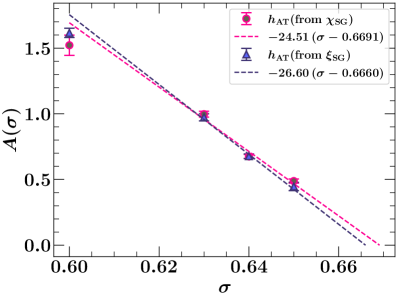
Figure 3: Plot of $A(\sigma)$ versus $\sigma$. The quantity $A(\sigma)$ is computed using Eq. (1) with the exponent $\zeta$ given by Eq. (16) in the mean-field regime. In our simulations we fixed the temperature $T=0.675T_{c}$ and determined the value of the transition field $h_{\text{AT}}$ from the $\chi_{\text{SG}}$ and $\xi_{\text{SG}}$ data sets, (for example see Fig. 2). So, for each $\sigma$, we get two values of $A(\sigma)$ corresponding to the two different values of $h_{\text{AT}}$. The $A(\sigma)$ data corresponding to $\sigma=0.630,0.640,\text{ and }0.650$ are fitted with a straight line. The red and blue lines intersect the $\sigma$ – axis at $\sigma=0.669\pm 0.072$ and $\sigma=0.666\pm 0.101$ respectively. In making these linear fits the data point at $\sigma=0.60$ has been ignored, as it probably lies outside the linear region.

The extent to which this linear fit works is shown in Fig. 2(c). From it we can make estimates of the value of $h_{\text{AT}}$. We get two estimates of its value; one from $\chi_{\text{SG}}$ and one from $\xi_{\text{SG}}$. From it, one can extract (using Eq. (1)) $A(\sigma)$ at the values of $\sigma$ which we have studied. We take the exponent to be:

$$\zeta=\begin{cases}3,&\;\;\sigma<5/8,\\[2.84544pt] \dfrac{2(1-\sigma)}{2\sigma-1},&\;\;5/8<\sigma<2/3,\end{cases}$$ (16)

where we have set $d=d_{\text{eff}}$ in $\zeta=d/2-1$ for $\sigma>5/8$ (Green et al., 1983; Fisher and Sompolinsky, 1985). We have plotted the results in Fig. 3. Clearly $A(\sigma)$ is decreasing with increasing $\sigma$, and in this linear plot it appears to go to zero when $\sigma\approx 0.67$. This is close to the value $2/3$ which is what would be expected if the AT line disappears in exactly $6$ dimensions.

When we studied $\sigma=0.655$, we saw a deviation from the straight line which goes through $\sigma\approx 0.67$ (see Fig. S9 of the Supplementary Material). We believe the basic reason for this deviation are finite size problems. Finite size effects give an apparent AT transition at values of $\sigma$ where it is actually absent! In our study of the XY model Vedula et al. (2023) we also studied the cases $\sigma=0.70,0.75\;\text{and}\;0.85$. These correspond to dimensions $d<6$ and in the region where the droplet scaling approach should work and where there will be no AT transition. However, there were still intersections of the lines of $\chi_{\text{SG}}$ and $\xi_{\text{SG}}$ for different $N$ values which at first sight suggests the presence of an AT transition and a non-vanishing value of $h_{\text{AT}}$. However, by studying the $N$ dependence of these intersections one could see that they do not correspond to a phase transition but are consequences of finite size effects. We believe that is why an AT transition was reported in the recent study in which a system with $d=6$ was simulated  Aguilar-Janita et al. (2023) and why the data point at $\sigma=0.655$ should be discounted.

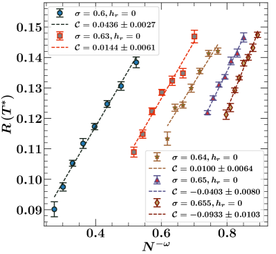
Figure 4: The values of $R(T^{*})=\chi_{\text{SG}}(T^{*}(N,2N),N)/N^{1/3}$ for the range of $\sigma$ values studied in this paper, in zero field. The correction to scaling exponent $\omega=1/3-(2\sigma-1)$. $\mathcal{C}$ is the value of $R$ obtained using the dotted line extrapolation. As $\sigma\to 2/3$ the values of $N$ needed to estimate the value of $R$ accurately in the thermodynamic limit increase rapidly.

To appreciate the size of finite size corrections it is useful to study $R$ where

$$R\equiv\frac{\chi_{\text{SG}}(T^{*}(N,2N),N)}{N^{1/3}}.$$ (17)

$R$ is essentially the righthand side of Eq. (12), if $T^{*}(N,2N)$ is close to $T_{c}$. Because we only determine $\chi_{\text{SG}}(T,N)$ at a finite number of values of $T$, we use linear interpolation to calculate $\chi_{\text{SG}}(T^{*}(N,2N),N)$ using the two points which lie on either side of $T^{*}(N,2N)$. $R$ should approach a positive constant as $1/N^{\omega}\to 0$. Fig. 4 shows that $1/N^{\omega}$ is still quite large at the system sizes which have been achieved in this study: The extrapolated value of $R$ for $N\to\infty$ are not even positive for the two values of $\sigma$ closest to $2/3$, i.e. 0.650 and 0.655. The magnitude of the scaling corrections in a field is very similar to the zero field case and the absence of good straight line fits in Fig. 2(c) is therefore to be expected. The system sizes studied are not sufficiently large to see the simple finite size scaling forms cleanly emerging.

Numerical studies like this can only provide evidence for what the truth might be: they do not as yet prove it beyond reasonable doubt. The controversy will probably only be ended by a rigorous determination of the lower critical dimension of the AT transition.

See pages 1, of sm.pdf See pages 0, of sm.pdf

References

- Parisi (1979) G. Parisi, Toward a mean field theory for spin glasses, Physics Letters A 73, 203 (1979).
- Mézard et al. (1986) M. Mézard, G. Parisi, and M. A. Virasoro, Spin glass theory and beyond: An Introduction to the Replica Method and Its Applications, Vol. 9 (World Scientific Publishing Company, 1986).
- Bray and Roberts (1980) A. J. Bray and S. A. Roberts, Renormalisation-group approach to the spin glass transition in finite magnetic fields, Journal of Physics C: Solid State Physics 13, 5405 (1980).
- de Almeida and Thouless (1978) J. R. L. de Almeida and D. J. Thouless, Stability of the Sherrington-Kirkpatrick solution of a spin glass model, Journal of Physics A: Mathematical and General 11, 983 (1978).
- Sherrington and Kirkpatrick (1975) D. Sherrington and S. Kirkpatrick, Solvable Model of a Spin-Glass, Phys. Rev. Lett. 35, 1792 (1975).
- Green et al. (1983) J. E. Green, M. A. Moore, and A. J. Bray, Upper critical dimension for the de Almeida-Thouless instability in spin glasses, Journal of Physics C: Solid State Physics 16, L815 (1983).
- Fisher and Sompolinsky (1985) D. S. Fisher and H. Sompolinsky, Scaling in Spin-Glasses, Phys. Rev. Lett. 54, 1063 (1985).
- Harris et al. (1976) A. B. Harris, T. C. Lubensky, and J.-H. Chen, Critical Properties of Spin-Glasses, Phys. Rev. Lett. 36, 415 (1976).
- Sharma and Young (2010) A. Sharma and A. P. Young, de Almeida–Thouless line in vector spin glasses, Phys. Rev. E 81, 061115 (2010).
- Moore and Bray (1985) M. A. Moore and A. J. Bray, The nature of the spin-glass phase and finite size effects, Journal of Physics C: Solid State Physics 18, L699 (1985).
- Yeo and Moore (2015) J. Yeo and M. A. Moore, Critical point scaling of Ising spin glasses in a magnetic field, Phys. Rev. B 91, 104432 (2015).
- Moore (2012) M. A. Moore, expansion in spin glasses and the de Almeida-Thouless line, Phys. Rev. E 86, 031114 (2012).
- Mattsson et al. (1995) J. Mattsson, T. Jonsson, P. Nordblad, H. Aruga Katori, and A. Ito, No Phase Transition in a Magnetic Field in the Ising Spin Glass FMTi, Phys. Rev. Lett. 74, 4305 (1995).
- Zotev et al. (2002) V. S. Zotev, G. G. Kenning, and R. Orbach, From linear to nonlinear response in spin glasses: Importance of mean-field-theory predictions, Phys. Rev. B 66, 014412 (2002).
- Martin-Mayor et al. (2022) V. Martin-Mayor, J. J. Ruiz-Lorenzo, B. Seoane, and A. P. Young, Numerical Simulations and Replica Symmetry Breaking (2022), arXiv:2205.14089 [cond-mat.dis-nn] .
- Aguilar-Janita et al. (2023) M. Aguilar-Janita, V. Martin-Mayor, J. Moreno-Gordo, and J. J. Ruiz-Lorenzo, Second order phase transition in the six-dimensional Ising spin glass on a field (2023), arXiv:2306.00569 [cond-mat.dis-nn] .
- Katzgraber and Young (2003) H. G. Katzgraber and A. P. Young, Monte Carlo studies of the one-dimensional Ising spin glass with power-law interactions, Phys. Rev. B 67, 134410 (2003).
- Leuzzi et al. (2008) L. Leuzzi, G. Parisi, F. Ricci-Tersenghi, and J. J. Ruiz-Lorenzo, Dilute One-Dimensional Spin Glasses with Power Law Decaying Interactions, Phys. Rev. Lett. 101, 107203 (2008).
- Sharma and Young (2011) A. Sharma and A. P. Young, Phase transitions in the one-dimensional long-range diluted Heisenberg spin glass, Phys. Rev. B 83, 214405 (2011).
- Vedula et al. (2023) B. Vedula, M. A. Moore, and A. Sharma, Study of the de Almeida–Thouless line in the one-dimensional diluted power-law spin glass, Phys. Rev. E 108, 014116 (2023).
- Lee and Young (2007) L. W. Lee and A. P. Young, Large-scale Monte Carlo simulations of the isotropic three-dimensional Heisenberg spin glass, Phys. Rev. B 76, 024405 (2007).
- Larson et al. (2010) D. Larson, H. G. Katzgraber, M. A. Moore, and A. P. Young, Numerical studies of a one-dimensional three-spin spin-glass model with long-range interactions, Phys. Rev. B 81, 064415 (2010).