Adaptive Backstepping Control of a Bicopter
in Pure Feedback Form with Dynamic Extension

Abstract

This paper presents a model-based, adaptive, nonlinear controller for the bicopter stabilization and trajectory-tracking problem. The nonlinear controller is designed using the backstepping technique. Due to the non-invertibility of the input map, the bicopter system is first dynamically extended. However, the resulting dynamically extended system is in the pure feedback form with the uncertainty appearing in the input map. The adaptive backstepping technique is then extended and applied to design the controller. The proposed controller is validated in simulation for a smooth and nonsmooth trajectory-tracking problem.

keywords: adaptive backstepping control, dynamic extension, bicopter, multicopter.

I INTRODUCTION

Multicopters have been widely used in several engineering applications such as precision agriculture [1], environmental survey [2, 3], construction management [4] and load transportation [5]. This popularity has also sparked interest in broadening their capacities and applications. Nonetheless, due to nonlinear, time-varying, unmodeled dynamics, unknown operating environments, and evermore demanding applications, reliable multicopter control remains a challenging problem.

Various control techniques have been applied to design control systems for multicopters [6, 7, 8]. Nevertheless, these techniques require prior knowledge of model parameters and, thus, are sensitive to physical model parameter uncertainty [9, 10]. Several adaptive control techniques have been applied to address the problem of unmodeled, unknown, and uncertain dynamics, such as model reference adaptive control [11, 12], L1 adaptive control [13], adaptive sliding mode control [14, 15, 16], retrospective cost adaptive control [17, 18]. These approaches either require an existing stabilizing controller or do not provide stability guarantees.

Modern control architectures decompose the multicopter’s nonlinear dynamics into outer-loop translational dynamics and the inner-loop rotational dynamics [19]. Note that the translation dynamics is linear and the rotational dynamics is nonlinear. Stabilizing controllers are then designed for each loop separately. However, the cascaded multiloop architecture does not guarantee the stability of the entire closed-loop system. The multi-loop architecture is motivated by the time separation principle, which is applicable in a scenario where each successive inner feedback loop is sufficiently faster than the previous outer loop. A stabilizing controller can be designed for each loop with appropriate transient behavior in such a case to satisfy the time separation principle. This crucial fact allows the multicopter dynamics to be decoupled and stabilizing controllers designed for each loop. Although the controller design is considerably simplified, the closed-loop stability can not be guaranteed.

This paper considers the problem of designing an adaptive controller for the fully coupled nonlinear dynamics of a multicopter. To focus on the controller design process, we consider a bicopter system, which is special case of a multicopter system. A bicopter is constrained to a vertical plane and thus is modeled by a 6th-order nonlinear instead of a 12th-order nonlinear system. Despite the lower dimension of the state space, the 6th-order bicopter retains the complexities of the nonlinear dynamics of an unconstrained multicopter. In this paper, we design an adaptive controller based on the backstepping technique [20]. However, the classical backstepping technique can not be applied due to the input map’s non invertibility. To circumvent this problem, the bicopter dynamics is first dynamically extended [21] Although the input map of the resulting extended system is invertible, the extended dynamics can only be expressed in the pure feedback form. Backstepping technique has been extended to design controllers for a system in pure feedback form in [22, 23, 24]. An adaptive extension of the backstepping technique for a pure feedback system was presented in [25]. However, [25] considers the case where uncertainty is in the dynamics map. As shown in Section III-B, the uncertainty in the bicopter dynamics appears in the input map. The contributions of this paper are thus 1) the design of an adaptive backstepping controller for the fully nonlinear bicopter system without decoupling the nonlinear system into simpler subsystems 2) extension of the backstepping control of pure feedback system to the case of uncertain input maps, and 3) validation of the proposed controller in a smooth and nonsmooth trajectory-tracking problem.

The paper is organized as follows. Section II derives the equation of motion of the bicopter system. Section III describes the adaptive backstepping procedure to design the adaptive controller for the bicopter. Section IV describes a numerical simulation to validate the adaptive controller. Finally, the paper concludes with a discussion of results and future research directions in section V.

II Bicopter Dynamics

Let ${\rm F_{A}}=\{\hat{\imath}_{\rm A},\hat{\jmath}_{\rm A},\hat{k}_{\rm A}\}$ be an inertial frame and let ${\rm F_{B}}=\{\hat{\imath}_{\rm B},\hat{\jmath}_{\rm B},\hat{k}_{\rm B}\}$ be a frame fixed to the bicopter ${\mathcal{B}}$ as shown in Figure 1. The bicopter ${\mathcal{B}}$ is constrained to move in the $\hat{\imath}_{\rm A}-\hat{\jmath}_{\rm A}$ plane. Note that $\rm F_{B}$ is obtained by rotating it about the $\hat{k}_{\rm A}$ axis of $\rm F_{A}$ by $\theta,$ and thus

$${\rm F_{A}}{\begin{subarray}{c}\theta\\ {\boldsymbol{\longrightarrow}}\\ 3\end{subarray}}{\rm F_{B}}.$$ (1)

Figure 1: Bicopter configuration considered in this paper. The bicopter is constrained to the $\hat{\hat{\imath}}_{\rm A}-\hat{\hat{\jmath}}_{\rm A}$ plane and rotates about the $\hat{k}_{\rm A}$ axis of the inertial frame $\rm F_{A}.$

Letting ${\rm c}$ denote the center of mass of the bicopter and $w$ denote a fixed point on Earth, it follows from Newton’s second law that

$$m\stackrel{{\scriptstyle{\rm A}\bullet\bullet}}{{\overset{\rightharpoonup}{r}}}_{{\rm c}/w} =m\overset{\rightharpoonup}{g}+\overset{\rightharpoonup}{f},$$ (2)

where $m$ is the mass of the bicopter, $\overset{\rightharpoonup}{g}$ is the acceleration due to gravity, and $\overset{\rightharpoonup}{f}$ is the total force applied by the propellers to the bicopter. Letting $\overset{\rightharpoonup}{f}_{1}=f_{1}\hat{\jmath}_{\rm B}$ and $\overset{\rightharpoonup}{f}_{2}=f_{2}\hat{\jmath}_{\rm B}$ denote the forces applied by the two propellers, it follows that $\overset{\rightharpoonup}{f}=f_{1}\hat{j}_{\rm B}+f_{2}\hat{j}_{\rm B}$. Writing $\overset{\rightharpoonup}{r}_{{\rm c}/w}=r_{1}\hat{\imath}_{\rm A}+r_{2}\hat{\jmath}_{\rm A}$ yields

$$m\ddot{r}_{1} =-(f_{1}+f_{2})\sin\theta,$$ (3)

$$m\ddot{r}_{2} =(f_{1}+f_{2})\cos\theta-mg.$$ (4)

Next, it follows from Euler’s equation that

$$\overset{\rightarrow}{J}_{{\mathcal{B}}/{\rm c}}\stackrel{{\scriptstyle{\rm A}\bullet\bullet}}{{\overset{\rightharpoonup}{\omega}}}_{\rm B/A}=\overset{\rightharpoonup}{M}_{{\mathcal{B}}/{\rm c}},$$ (5)

where $\overset{\rightarrow}{J}_{{\mathcal{B}}/{\rm c}}$ is the physical inertia matrix and $\overset{\rightharpoonup}{M}_{{\mathcal{B}}/{\rm c}}$ is the moment applied to ${\mathcal{B}}$ about the point ${\rm c}.$ Note that $\overset{\rightarrow}{J}_{{\mathcal{B}}/{\rm c}}\stackrel{{\scriptstyle{\rm A}\bullet\bullet}}{{\overset{\rightharpoonup}{\omega}}}_{\rm B/A}=J\ddot{\theta}\hat{k}_{\rm B}$ and $\overset{\rightharpoonup}{M}_{{\mathcal{B}}/{\rm c}}=\ell(f_{2}-f_{1})\hat{k}_{\rm B},$ where $\ell$ is the length of the bicopter arm, and thus it follows from (5) that

$$J\ddot{\theta}=\ell(f_{2}-f_{1}).$$ (6)

Defining

$$F \stackrel{{\scriptstyle\triangle}}{{=}}f_{1}+f_{2},$$ (7)

$$M \stackrel{{\scriptstyle\triangle}}{{=}}(-f_{1}+f_{2})\ell,$$ (8)

it follows that

$$m\ddot{r}_{1} =-F\sin\theta,$$ (9)

$$m\ddot{r}_{2} =F\cos\theta-mg,$$ (10)

$$J\ddot{\theta} =M.$$ (11)

III Adaptive Backstepping Control

In this section, we construct an adaptive backstepping controller to stabilize the bicopter system. To do so, the equations of motion, given by (9)-(11), must be reformulated into the strict feedback form to apply the classical backstepping. However, as shown below, the classical backstepping technique is not applicable due to the singularity of the input map.

III-A Strict Feedback Form of Bicopter Dynamics

Defining

$$x_{1}\stackrel{{\scriptstyle\triangle}}{{=}}\begin{bmatrix}r_{1}\\ r_{2}\\ \theta\end{bmatrix},x_{2}\stackrel{{\scriptstyle\triangle}}{{=}}\begin{bmatrix}\dot{r}_{1}\\ \dot{r}_{2}\\ \dot{\theta}\end{bmatrix},u \stackrel{{\scriptstyle\triangle}}{{=}}\begin{bmatrix}F\\ M\end{bmatrix},\Theta\stackrel{{\scriptstyle\triangle}}{{=}}\begin{bmatrix}m^{-1}\\ J^{-1}\end{bmatrix}$$ (12)

it follows that

$$\dot{x}_{1} =x_{2},$$ (13)

$$\dot{x}_{2} =f_{2}(x_{1},x_{2})+g_{2}(x_{1},x_{2}){\rm diag}(\Theta)\,u,$$ (14)

where

$$f_{2}(x_{1},x_{2})\stackrel{{\scriptstyle\triangle}}{{=}}\begin{bmatrix}0\\ -g\\ 0\end{bmatrix},\quad g_{2}(x_{1},x_{2})\stackrel{{\scriptstyle\triangle}}{{=}}\begin{bmatrix}-\sin(x_{1,3})&0\\ \cos(x_{1,3})&0\\ 0&1\end{bmatrix}.$$ (15)

Note that the map $g_{2}$ is not invertible; hence, classical backstepping [20, p. 29] can not be applied to this system.

III-B Dynamic Extension of Bicopter Dynamics

To circumvent the problem of the singularity of the input map, we extend the dynamics as shown below. Redefining

$$x_{1}\stackrel{{\scriptstyle\triangle}}{{=}}\begin{bmatrix}r_{1}\\ r_{2}\end{bmatrix},\ x_{2}\stackrel{{\scriptstyle\triangle}}{{=}}\begin{bmatrix}\dot{r}_{1}\\ \dot{r}_{2}\end{bmatrix},\ x_{3}\stackrel{{\scriptstyle\triangle}}{{=}}\begin{bmatrix}F\\ \theta\end{bmatrix},\ x_{4}\stackrel{{\scriptstyle\triangle}}{{=}}\begin{bmatrix}\dot{F}\\ \dot{\theta}\end{bmatrix},$$ (16)

and

$$u\stackrel{{\scriptstyle\triangle}}{{=}}\begin{bmatrix}\ddot{F}\\ M\end{bmatrix},\quad\Theta\stackrel{{\scriptstyle\triangle}}{{=}}\begin{bmatrix}\Theta_{1}\\ \Theta_{2}\end{bmatrix}=\begin{bmatrix}m^{-1}\\ J^{-1}\end{bmatrix},$$ (17)

it follows from the equations of motion (3), (4), and (6) that

$$\dot{x}_{1} =x_{2},$$ (18)

$$\dot{x}_{2} =f_{2}(x_{1},x_{2})+g_{2}(x_{3})\Theta_{1},$$ (19)

$$\dot{x}_{3} =x_{4},$$ (20)

$$\dot{x}_{4} ={\rm diag}(1,\Theta_{2})u,$$ (21)

where

$$f_{2}(x_{1},x_{2}) \stackrel{{\scriptstyle\triangle}}{{=}}\begin{bmatrix}0\\ -g\end{bmatrix},\quad g_{2}(x_{3})\stackrel{{\scriptstyle\triangle}}{{=}}\begin{bmatrix}-\sin(x_{3,2})x_{3,1}\\ \cos(x_{3,2})x_{3,1}\end{bmatrix}.$$ (22)

Note that the dynamic extension of the bicopter system, given by (18)-(21), is not in the desired strict feedback form. In fact, the extended dynamics is in pure feedback form since $x_{3}$ appears non-affinely in (19). However, since the input map ${\rm diag}(1,\Theta_{2})$ is invertible, and thus the backstepping technique can now be applied to the extended system to construct a controller.

III-C Adaptive Backstepping-based Control of Bicopter

Next, we construct an adaptive controller based on the backstepping technique. This approach is based on the process described in [20, p. 29].

III-C1 $e_{1}$ Stabilization

Let $x_{1{\rm d}}=\begin{bmatrix}r_{{\rm d}1}&r_{{\rm d}2}\end{bmatrix}^{\rm T}$ denote the desired trajectory, and define the tracking error $e_{1}\stackrel{{\scriptstyle\triangle}}{{=}}x_{1}-x_{1{\rm d}}.$ Consider the function

$$V_{1}\stackrel{{\scriptstyle\triangle}}{{=}}\frac{1}{2}e_{1}^{\rm T}e_{1}.$$ (23)

Differentiating (23) and using (18) yields

$$\dot{V}_{1}=e_{1}^{\rm T}\dot{x}_{1}=e_{1}^{\rm T}x_{2}.$$ (24)

Note that if $x_{2}=-k_{1}e_{1},$ where $k_{1}>0,$ then $\dot{V}_{1}<0.$ However, $x_{2}$ is not the control signal and thus can not be chosen arbitrarily. Instead, following the backstepping process, we design a control law that yields the desired $x_{2}$ response, as shown below.

III-C2 $e_{2}$ Stabilization

Next, consider the function

$$V_{2}\stackrel{{\scriptstyle\triangle}}{{=}}V_{1}+\frac{1}{2}e_{2}^{\rm T}e_{2},$$ (25)

where

$$e_{2} \stackrel{{\scriptstyle\triangle}}{{=}}x_{2}-x_{2{\rm d}},$$ (26)

$$x_{2{\rm d}} \stackrel{{\scriptstyle\triangle}}{{=}}-k_{1}e_{1}.$$ (27)

Differentiating (25) and using (19) yields

$$\dot{V}_{2} =-k_{1}e_{1}^{\rm T}e_{1}+e_{2}^{\rm T}\xi_{2},$$ (28)

where

$$\xi_{2}\stackrel{{\scriptstyle\triangle}}{{=}}x_{1}+f_{2}+g_{2}\Theta_{1}+k_{1}x_{2}.$$ (29)

Note that if

$$g_{2}(x_{3})\Theta_{1}=-e_{2}-e_{1}-f_{2}-k_{1}x_{2},$$ (30)

then $\dot{V}_{2}<0.$

Let $\hat{\Theta}_{1}$ be an estimate of $\Theta_{1},$ and define $\tilde{\Theta}_{1}\stackrel{{\scriptstyle\triangle}}{{=}}\hat{\Theta}_{1}-\Theta_{1}.$ Next, define

$$x_{3{\rm d}} \stackrel{{\scriptstyle\triangle}}{{=}}x_{3}-(g_{2}\tilde{\Theta}_{1}+\xi_{2})-k_{2}e_{2},$$ (31)

$$e_{3} \stackrel{{\scriptstyle\triangle}}{{=}}x_{3}-x_{3{\rm d}},$$ (32)

where $k_{2}>0,$ which implies that

$$\xi_{2} =e_{3}-g_{2}\tilde{\Theta}_{1}-k_{2}e_{2}\in{\mathbb{R}}^{2}.$$ (33)

Substituting (33) in (28) yields

$$\dot{V}_{2} =-k_{1}e_{1}^{\rm T}e_{1}-k_{2}e_{2}^{\rm T}e_{2}+e_{2}^{\rm T}\left(e_{3}+g_{2}(\Theta_{1}-\hat{\Theta}_{1})\right).$$ (34)

III-C3 $\Theta_{1}$ Adaptation

Next, consider the function

$${\mathcal{V}}_{2}\stackrel{{\scriptstyle\triangle}}{{=}}V_{2}+\frac{1}{2}\gamma_{1}^{-1}(\Theta_{1}-\hat{\Theta}_{1})^{\rm T}(\Theta_{1}-\hat{\Theta}_{1})$$ (35)

where $\gamma_{1}>0.$ Differentiating (35) yields

$$\dot{\mathcal{V}}_{2} =-k_{1}e_{1}^{\rm T}e_{1}-k_{2}e_{2}^{\rm T}e_{2}+e_{2}^{\rm T}e_{3}+$$

$$\quad(\Theta_{1}-\hat{\Theta}_{1})^{\rm T}\left(g_{2}^{\rm T}e_{2}-\gamma_{1}^{-1}\dot{\hat{\Theta}}_{1}\right).$$ (36)

Letting

$$\dot{\hat{\Theta}}_{1}=\gamma_{1}g_{2}^{\rm T}e_{2}$$ (37)

yields

$$\dot{\mathcal{V}}_{2} =-k_{1}e_{1}^{\rm T}e_{1}-k_{2}e_{2}^{\rm T}e_{2}+e_{2}^{\rm T}e_{3}.$$ (38)

III-C4 $e_{3}$ Stabilization

Next, consider the function

$$V_{3}\stackrel{{\scriptstyle\triangle}}{{=}}{\mathcal{V}}_{2}+\frac{1}{2}e_{3}^{\rm T}e_{3}.$$ (39)

Note that

$$\dot{\xi}_{2} =x_{2}+{\mathcal{G}}_{2}\Theta_{1}+k_{1}(f_{2}+g_{2}\Theta_{1}),$$ (40)

where

$${\mathcal{G}}_{2}\stackrel{{\scriptstyle\triangle}}{{=}}{\partial_{x_{3}}g_{2}}=\begin{bmatrix}-\cos(x_{3,2})x_{3,1}&-\sin(x_{3,2})\\ -\sin(x_{3,2})x_{3,1}&\cos(x_{3,2})\end{bmatrix}.$$ (41)

Differentiating (39) and using (20), (31) and (40) yields

$$\dot{V}_{3} =-k_{1}e_{1}^{\rm T}e_{1}-k_{2}e_{2}^{\rm T}e_{2}+e_{3}^{\rm T}\xi_{3}$$ (42)

where

$$\xi_{3} \stackrel{{\scriptstyle\triangle}}{{=}}2x_{2}+k_{1}e_{1}+{\mathcal{G}}_{2}x_{4}\hat{\Theta}_{1}$$

$$\quad+\gamma_{1}g_{2}g_{2}^{\rm T}e_{2}+\kappa_{12}(f_{2}+g_{2}{\Theta}_{1})+k_{1}k_{2}x_{2}.$$ (43)

and $\kappa_{12}\stackrel{{\scriptstyle\triangle}}{{=}}k_{1}-k_{2}.$

Let $\hat{\vartheta}_{1}$ be an estimate of $\Theta_{1},$ and define $\tilde{\vartheta}_{1}\stackrel{{\scriptstyle\triangle}}{{=}}\hat{\vartheta}_{1}-\Theta_{1}.$ Next, define

$$x_{4{\rm d}} \stackrel{{\scriptstyle\triangle}}{{=}}x_{4}-\Big{(}\kappa_{12}g_{2}\tilde{\vartheta}_{1}+\xi_{3}\Big{)}-k_{3}e_{3},$$ (44)

where $k_{3}>0,$ and $\hat{\vartheta}_{1}$ is given by the adaptation law (50). Rearranging (44) yields

$$\xi_{3} =e_{4}-\kappa_{12}g_{2}\tilde{\vartheta}_{1}-k_{3}e_{3}\,\in\mathbb{R}^{2},$$ (45)

where

$$e_{4}\stackrel{{\scriptstyle\triangle}}{{=}}x_{4}-x_{4{\rm d}}.$$ (46)

Substituting (45) in (42) yields

$$\dot{V}_{3} =-k_{1}e_{1}^{\rm T}e_{1}-k_{2}e_{2}^{\rm T}e_{2}-k_{3}e_{3}^{\rm T}e_{3}+e_{3}^{\rm T}e_{4}$$

$$\quad-e_{3}^{\rm T}\kappa_{12}g_{2}\tilde{\vartheta}_{1}.$$ (47)

III-C5 $\vartheta_{1}$ Adaptation

Next, consider the function

$${\mathcal{V}}_{3} \stackrel{{\scriptstyle\triangle}}{{=}}V_{3}+\dfrac{1}{2}\gamma_{2}^{-1}\tilde{\vartheta}_{1}^{\rm T}\tilde{\vartheta}_{1},$$ (48)

where $\gamma_{2}>0.$ Differentiating (48) yields

$$\dot{{\mathcal{V}}}_{3} =-k_{1}e_{1}^{\rm T}e_{1}-k_{2}e_{2}^{\rm T}e_{2}-k_{3}e_{3}^{\rm T}e_{3}+e_{3}^{\rm T}e_{4}$$

$$\quad-\Big{(}\kappa_{12}g_{2}^{\rm T}e_{3}-\gamma_{2}^{-1}\dot{\hat{\vartheta}}_{1}\Big{)}\tilde{\vartheta}_{1}.$$ (49)

Letting

$$\dot{\hat{\vartheta}}_{1}=\gamma_{2}\kappa_{12}g_{2}(x_{3})^{\rm T}e_{3},$$ (50)

yields

$$\dot{{\mathcal{V}}}_{3} =-k_{1}e_{1}^{\rm T}e_{1}-k_{2}e_{2}^{\rm T}e_{2}-k_{3}e_{3}^{\rm T}e_{3}+e_{3}^{\rm T}e_{4}.$$ (51)

III-C6 $e_{4}$ Stabilization

Next, consider the function

$$V_{4} \stackrel{{\scriptstyle\triangle}}{{=}}{\mathcal{V}}_{3}+\dfrac{1}{2}e_{4}^{\rm T}e_{4}.$$ (52)

Differentiating (52) and using (21) yields

$$\dot{V}_{4} =-k_{1}e_{1}^{\rm T}e_{1}-k_{2}e_{2}^{\rm T}e_{2}-k_{3}e_{3}^{\rm T}e_{3}+e_{4}^{\rm T}\xi_{4},$$ (53)

where

$$\xi_{4} \stackrel{{\scriptstyle\triangle}}{{=}}\Bigg{(}x_{1}+3f_{2}+g_{2}\hat{\Theta}_{1}+2k_{1}x_{2}$$

$$\quad+k_{2}\left(x_{2}+k_{1}e_{1}\right)+2g_{2}\Theta_{1}$$

$$\quad+\dfrac{d}{dt}\left[\dfrac{\partial g(x_{3})}{\partial x_{3}}\right]x_{4}\hat{\Theta}_{1}$$

$$\quad+{\mathcal{G}}_{2}\text{diag}(1,\Theta_{2})\hat{\Theta}_{1}u+2{\mathcal{G}}_{2}x_{4}\dot{\hat{\Theta}}_{1}$$

$$\quad+\gamma_{1}g_{2}\Bigg{[}x_{4}^{\rm T}{\mathcal{G}}_{2}^{\rm T}\left(x_{2}+k_{1}e_{1}\right)$$

$$\quad+g_{2}^{\rm T}\left(f_{2}+g_{2}\Theta_{1}+k_{1}x_{2}\right)\Bigg{]}$$

$$\quad+K_{12}{\mathcal{G}}_{2}x_{4}\hat{\vartheta}_{1}$$

$$\quad+K_{12}g_{2}\dot{\hat{\vartheta}}_{1}+k_{1}k_{2}\left(f_{2}+g_{2}\Theta_{1}\right)$$

$$\quad+k_{3}\Bigg{(}x_{2}+{\mathcal{G}}_{2}x_{4}\hat{\Theta}_{1}+g_{2}\dot{\hat{\Theta}}_{1}$$

$$\quad+K_{12}\left(f_{2}+g_{2}\Theta_{1}\right)+k_{1}k_{2}x_{2}\Bigg{)}\Bigg{)}$$ (54)

where $K_{12}\stackrel{{\scriptstyle\triangle}}{{=}}k_{1}+k_{2}.$

Note that if

$$\xi_{4}=-k_{4}e_{4},$$ (55)

where $k_{4}>0$. Then,

$$\dot{V}_{4} =-k_{1}e_{1}^{\rm T}e_{1}-k_{2}e_{2}^{\rm T}e_{2}-k_{3}e_{3}^{\rm T}e_{3}-k_{4}e_{4}^{\rm T}e_{4}<0.$$ (56)

Let $\hat{\varphi}_{1}$ and $\hat{\Theta}_{2}$ be an estimate of $\Theta_{1}$ and $\Theta_{2},$ respectively. Define $\tilde{\varphi}_{1}\stackrel{{\scriptstyle\triangle}}{{=}}\hat{\varphi}_{1}-\Theta_{1}$ and $\tilde{\Theta}_{2}\stackrel{{\scriptstyle\triangle}}{{=}}\hat{\Theta}_{2}-\Theta_{2}.$ Then, letting

$$u= -\left({\mathcal{G}}_{2}\text{diag}(1,\hat{\Theta}_{2})\hat{\Theta}_{1}\right)^{-1}\Bigg{(}k_{4}e_{4}+e_{3}$$

$$\quad+\left(k_{3}(k_{1}+k_{2})+k_{1}k_{2}+2+\gamma_{1}g_{2}~{}g_{2}^{\rm T}\right)\left(f_{2}+g_{2}\hat{\varphi}_{1}\right)$$

$$\quad+\left(k_{3}(k_{1}k_{2}+1)+k_{1}+\gamma_{1}g_{2}~{}g_{2}^{\rm T}\right)x_{2}$$

$$\quad+\left({\mathcal{G}}_{2}x_{4}-k_{3}g_{2}\right)\dot{\hat{\Theta}}_{1}+\left(\frac{{\rm d}}{\rm dt}{{\mathcal{G}}_{2}}+k_{3}{\mathcal{G}}_{2}\right)x_{4}\hat{\Theta}_{1}$$

$$\quad+K_{12}{\mathcal{G}}_{2}x_{4}\hat{\vartheta}_{1}+K_{12}g_{2}\dot{\hat{\vartheta}}_{1}$$

$$\quad+2\gamma_{1}{\mathcal{G}}_{2}x_{4}g_{2}^{\rm T}(x_{2}+k_{1}e_{1})\Bigg{)},$$ (57)

yields

$$\dot{V}_{4} =-k_{1}e_{1}^{\rm T}e_{1}-k_{2}e_{2}^{\rm T}e_{2}-k_{3}e_{3}^{\rm T}e_{3}-k_{3}e_{4}^{\rm T}e_{4}+e_{4}^{\rm T}\cdot$$

$$\quad\Bigg{[}-\left(k_{3}K_{12}+k_{1}k_{2}+2+\gamma_{1}g_{2}~{}g_{2}^{\rm T}\right)g_{2}\tilde{\varphi}_{1}$$

$$\quad-\hat{\Theta}_{1}{\mathcal{G}}_{2}\begin{bmatrix}0\\ u_{2}\end{bmatrix}\tilde{\Theta}_{2}\Bigg{]}$$ (58)

III-C7 $\hat{\varphi}_{1}$ and $\hat{\Theta}_{2}$ Adaptations

Next, consider the function

$${\mathcal{V}}_{4} =V_{4}+\dfrac{1}{2}\gamma_{3}^{-1}\tilde{\varphi}_{1}^{\rm T}\tilde{\varphi}_{1}+\dfrac{1}{2}\gamma_{4}^{-1}\tilde{\Theta}_{2}^{\rm T}\tilde{\Theta}_{2},$$ (59)

where $\gamma_{3}>0$ and $\gamma_{4}>0$. Differentiating (59) yields

$$\dot{{\mathcal{V}}}_{4}=-k_{1}e_{1}^{\rm T}e_{1}-k_{2}e_{2}^{\rm T}e_{2}-k_{3}e_{3}^{\rm T}e_{3}-k_{3}e_{4}^{\rm T}e_{4}$$

$$+\left(-e_{4}^{\rm T}\big{(}k_{3}K_{12}+k_{1}k_{2}+2+\gamma_{1}g_{2}~{}g_{2}^{\rm T}\big{)}g_{2}+\gamma_{3}^{-1}\dot{\hat{\varphi}}_{1}^{\rm T}\right)\tilde{\varphi}_{1}$$

$$+\left(-e_{4}^{\rm T}\hat{\Theta}_{1}{\mathcal{G}}_{2}\begin{bmatrix}0\\ u_{2}\end{bmatrix}+\gamma_{4}^{-1}\dot{\hat{\Theta}}_{2}^{\rm T}\right)\tilde{\Theta}_{2}.$$ (60)

Letting

$$\dot{\hat{\varphi}}_{1} =\gamma_{3}g_{2}^{\rm T}\big{(}k_{3}K_{12}+k_{1}k_{2}+2+\gamma_{1}g_{2}^{\rm T}g_{2}\big{)}e_{4},$$ (61)

$$\dot{\hat{\Theta}}_{2} =\gamma_{4}\hat{\Theta}_{1}\begin{bmatrix}0&u_{2}\end{bmatrix}{\mathcal{G}}_{2}^{\rm T}e_{4},$$ (62)

yields

$$\dot{{\mathcal{V}}}_{4} =-k_{1}e_{1}^{\rm T}x_{1}-k_{2}e_{2}^{\rm T}e_{2}-k_{3}e_{3}^{\rm T}e_{3}-k_{4}e_{4}^{\rm T}e_{4}.$$ (63)

The controller is thus given by (27), (31), (44), and (57) with the parameter adaption laws (37), (50), (61), and (62). The block diagram showing the architecture of the adaptive backstepping controller is shown in Figure 2.

Figure 2: Adaptive backstepping control architecture.

III-D Stability Analysis

Note that the control (57) requires ${\mathcal{G}}_{2}\text{diag}(1,\hat{\Theta}_{2})\hat{\Theta}_{1}$ to be nonsingular, which implies that ${\mathcal{G}}_{2}$ must be nonsingular and $\hat{\Theta}_{1},\hat{\Theta}_{2}\neq 0$. If $F\neq 0,$ which is reasonably expected during the system’s operation, ${\mathcal{G}}_{2}$ is nonsingular. However, the parameter adaptation laws do not ensure that $\hat{\Theta}_{1},\hat{\Theta}_{2}\neq 0.$ Thus, the global asymptotic stability of the closed-loop system can not be guaranteed.

Next, consider the function

$${\mathcal{V}}_{4}(e_{1},e_{2},e_{3},e_{4},\hat{\Theta}_{1},\hat{\vartheta}_{1},\hat{\varphi}_{1},\hat{\Theta}_{2})=\dfrac{1}{2}e_{1}^{\rm T}e_{1}+\dfrac{1}{2}e_{2}^{\rm T}e_{2}$$

$$\quad+\dfrac{1}{2}e_{3}^{\rm T}e_{3}+\dfrac{1}{2}e_{4}^{\rm T}e_{4}+\dfrac{1}{2}\gamma_{1}^{-1}\tilde{\Theta}_{1}^{\rm T}\tilde{\Theta}_{1}+\dfrac{1}{2}\gamma_{2}^{-1}\tilde{\vartheta}_{1}^{\rm T}\tilde{\vartheta}_{1}$$

$$\quad+\dfrac{1}{2}\gamma_{3}^{-1}\tilde{\varphi}_{1}^{\rm T}\tilde{\varphi}_{1}+\dfrac{1}{2}\gamma_{4}^{-1}\tilde{\Theta}_{2}^{\rm T}\tilde{\Theta}_{2},$$ (64)

where $\gamma_{1},\gamma_{2},\gamma_{3},\gamma_{4}>0.$ Let $D={\mathbb{R}}^{2}\times{\mathbb{R}}^{2}\times{\mathbb{R}}^{2}\times{\mathbb{R}}^{2}\times{\mathbb{R}}/\{0\}\times{\mathbb{R}}\times{\mathbb{R}}\times{\mathbb{R}}/\{0\}.$ Then, ${\mathcal{V}}_{4}(x)\geq 0$ for all $x\in D.$ Furthermore, it follows from (63) that $\dot{\mathcal{V}}_{4}\leq 0.$ Moreover, $\dot{\mathcal{V}}_{4}(x)=0$ if and only if $e_{1}=e_{2}=e_{3}=e_{4}=0.$ Let $E$ be the set of all points in $D$ such that $e_{1}=e_{2}=e_{3}=e_{4}=0.$ Note that $E$ is the largest positively invariant set with respect to (18)-(21) in $E.$ Then, it follows from the Barbashin-Krasovsky-La Salle’s invariance principle [26] that $e_{1},e_{2},e_{3},e_{4}\to 0.$

IV Simulations

In this section, we apply the adaptive backstepping controller developed in the previous section to the trajectory tracking problem. In particular, we use the adaptive controller to follow an elliptical and a second-order Hilbert curve based trajectory.

To simulate the bicopter, we assume that the mass of the bicopter is $1\ \rm kg$ and its inertia is $0.2$ $\rm kg\cdot m^{2}.$ In the controller, we set $k_{1}=5$, $k_{2}=5$, $k_{3}=4$, and $k_{4}=4$. In the adaptation laws, we set the adaptation gains $\gamma_{1}=1$, $\gamma_{2}=0.05$, $\gamma_{3}=0.05$, and $\gamma_{4}=0.1$, and the initial estimates $\hat{\Theta}_{1}(0)=0.5$, $\hat{\vartheta}_{1}(0)=0.5$, $\hat{\varphi}_{1}(0)=0.5$, and $\hat{\Theta}_{2}(0)=40$.

IV-A Elliptical Trajectory

The bicopter is commanded to follow a elliptical trajectory given by

$$r_{{\rm d}1}(t) =5\cos(\phi)-5\cos(\phi)\cos(\omega t)-3\sin(\phi)\sin(\omega t),$$

$$r_{{\rm d}2}(t) =5\sin(\phi)-5\sin(\phi)\cos(\omega t)+3\cos(\phi)\sin(\omega t),$$

where $\phi=45~{}\rm{deg}$ and $\omega=0.3\ \rm rad/s^{-1}.$ Figure 3 shows the trajectory-tracking response of the bicopter, where the desired trajectory is shown in black dashes and the output trajectory response is shown in blue. Figure 4 shows the position $r_{1},r_{2}$ response and the roll angle $\theta$ response of the bicopter with the adaptive backstepping controller. Figure 5 shows the norm of the position errors obtained with the adaptive backstepping controller on a logarithmic scale.

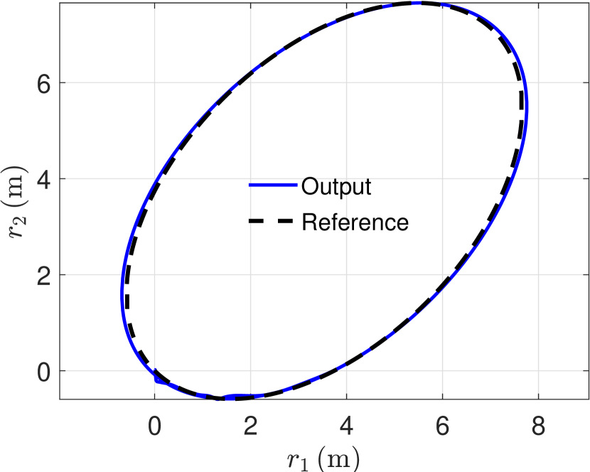
Figure 3: Elliptical trajectory. Tracking response of the bicopter with the adaptive backstepping controller. Note that the output trajectory is shown in solid blue, and the reference trajectory is in dashed black.

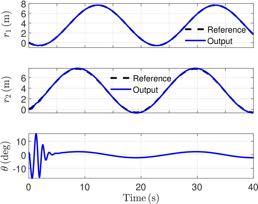
Figure 4: Elliptical trajectory. Position $(r_{1},r_{2})$ and roll angle $\theta$ response of the bicopter obtained with adaptive backstepping controller (57).

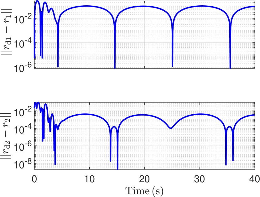
Figure 5: Elliptical trajectory. Position errors obtained with the adaptive backstepping controller (57) on a logarithmic scale.

Figure 6 shows the estimates $\hat{\Theta}_{1},\hat{\vartheta}_{1},$ and $\hat{\varphi}_{1}$ of $\Theta_{1}$ and the estimate $\hat{\Theta}_{2}$ of $\Theta_{2}.$ Note that the parameter estimates do not converge to their actual values. However, the non-convergence of the estimates is not due to persistency-related issues. In the adaptive controller design, since the parameter adaptation laws are chosen to cancel undesirable factors and not to estimate the parameters, the estimates do not necessarily need to converge. Finally, Figure 7 shows the control $u$ generated by the adaptive backstepping controller (57) and the corresponding forces $f_{1}$ and $f_{2}.$ Note that the forces $f_{1},f_{2}$ are computed using (7),and (8).

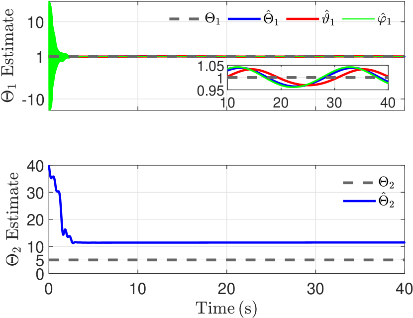
Figure 6: Elliptical trajectory. Estimates of $\Theta_{1}$ and $\Theta_{2}$ obtained with adaption laws (37), (50), (61), and (62).

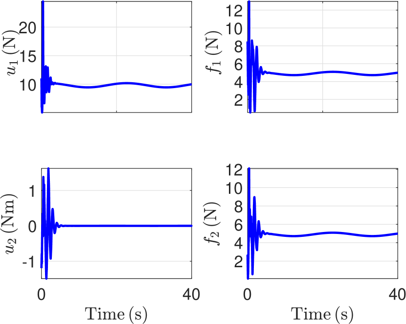
Figure 7: Elliptical trajectory. Control $u$ and the corresponding forces $f_{1}$ and $f_{2}$ obtained with adaptive backstepping controller (57).

IV-B Hilbert trajectory

Next, the bicopter is commanded to follow a nonsmooth trajectory constructed using a second-order Hilbert curve. The trajectory is constructed using the algorithm described in Appendix A of [27] with a maximum velocity $v_{\rm max}=1\ \rm m/s$ and a maximum acceleration $a_{\rm max}=1\ \rm m/s^{2}.$ Figure 8 shows the trajectory-tracking response of the bicopter, where the desired trajectory is shown in black dashes, and the output trajectory response is shown in blue. Figure 9 shows the position $r_{1}$ and $r_{2}$ response and the roll angle $\theta$ response of the bicopter with the adaptive backstepping controller. Figure 10 shows the norm of the position errors obtained with the adaptive backstepping controller on a logarithmic scale.

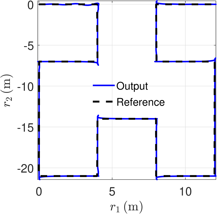
Figure 8: Hilbert trajectory. Tracking response of the bicopter with adaptive backstepping controller. Note that the output trajectory is in solid blue, and the desired trajectory is in dashed black.

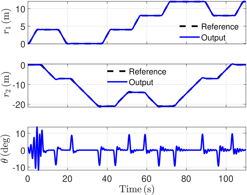
Figure 9: Hilbert trajectory. Positions $(r_{1},r_{2})$ and roll angle $\theta$ response of the bicopter with adaptive backstepping controller.

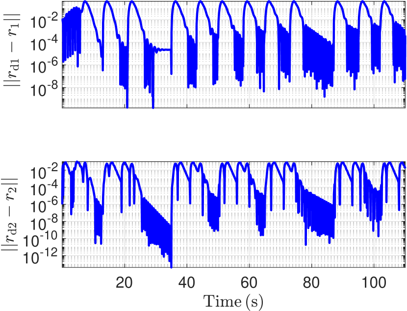
Figure 10: Hilbert trajectory. Position errors with the adaptive backstepping controller on a logarithmic scale.

Figure 11 shows the estimates $\hat{\Theta}_{1},\hat{\vartheta}_{1},$ and $\hat{\varphi}_{1}$ of $\Theta_{1}$ and the estimate $\hat{\Theta}_{2}$ of $\Theta_{2}.$ As in the previous case, note that the estimates do not converge to their actual values. Finally, Figure 12 shows the control $u$ generated by the adaptive backstepping controller (57), and the corresponding forces $f_{1}$ and $f_{2}$. Note that the forces $f_{1}$ and $f_{2}$ are computed using (7), and (8).

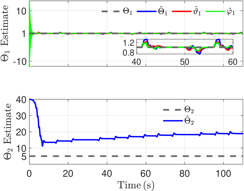
Figure 11: Hilbert trajectory. $\Theta_{1}$ and $\Theta_{2}$ Estimations with the adaptive backstepping controller. Note that the parameters used in the model are in dashed black.

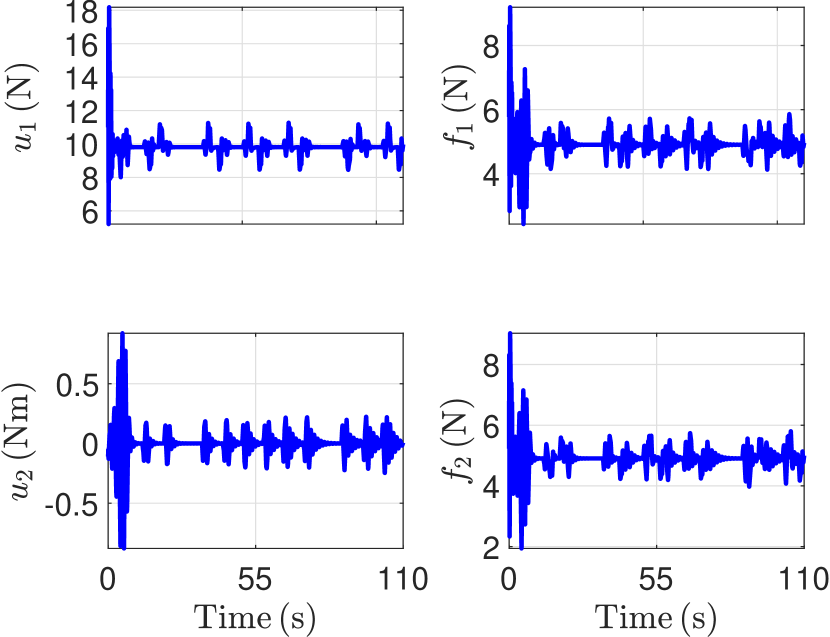
Figure 12: Hilbert trajectory. Control $u$ and the corresponding forces $f_{1}$ and $f_{2}$ obtained with adaptive backstepping controller.

The preceding two examples show that the adaptive backstepping controller stabilizes the bicopter dynamics and successfully tracks the desired trajectory without prior knowledge of the bicopter dynamics.

V Conclusions

This paper presented an adaptive backstepping-based controller for the stabilization and tracking problem in a bicopter system. It is shown that the backstepping process can not be applied to the bicopter dynamics due to the singularity of the input map. The bicopter dynamics is then dynamically extended to circumvent the singularity problem. The backstepping process is then used to stabilize the successive states of the extended bicopter system and design parameter adaption laws. Since the final control law requires the inversion of two of the parameter estimates, the global asymptotic stability of the closed-loop system cannot be guaranteed as the adaptation laws do not enforce a constraint on the estimate values. However, as shown in the numerical simulations, the closed-loop system is asymptotically stable with appropriately chosen gains, and the controller yields the desired tracking performance.

Future extensions will focus on 1) integrating constraints in the parameter adaption law that guarantees global stability of the closed-loop system for all gains chosen in the control law and the parameter adaptation laws, 2) reformulating the control laws as cascaded control, and finally, 3) extending the adaptive backstepping control presented in this paper to design a stabilizing and tracking controller for a quadcopter.

References

• [1] Anandarup Mukherjee, Sudip Misra and Narendra Singh Raghuwanshi “A survey of unmanned aerial sensing solutions in precision agriculture” In J. Netw. Comput. Appl. 148 Elsevier, 2019, pp. 102461
• [2] Arko Lucieer, Steven M de Jong and Darren Turner “Mapping landslide displacements using Structure from Motion (SfM) and image correlation of multi-temporal UAV photography” In Prog. Phys. Geogr. 38.1 Sage, 2014, pp. 97–116
• [3] Victor V Klemas “Coastal and environmental remote sensing from unmanned aerial vehicles: An overview” In J. Coast. Res. 31.5 The Coastal EducationResearch Foundation, 2015, pp. 1260–1267
• [4] Yan Li and Chunlu Liu “Applications of multirotor drone technologies in construction management” In Int. J. Constr. Manag. 19.5 Taylor & Francis, 2019, pp. 401–412
• [5] Daniel KD Villa, Alexandre S Brandao and Mário Sarcinelli-Filho “A survey on load transportation using multirotor UAVs” In J. Intell. Robot. Syst. 98 Springer, 2020, pp. 267–296
• [6] Tiago P Nascimento and Martin Saska “Position and attitude control of multi-rotor aerial vehicles: A survey” In Annu. Rev. Contr. 48 Elsevier, 2019, pp. 129–146
• [7] Julius A Marshall, Wei Sun and Andrea L’Afflitto “A survey of guidance, navigation, and control systems for autonomous multi-rotor small unmanned aerial systems” In Annu. Rev. Contr. 52 Elsevier, 2021, pp. 390–427
• [8] Pedro Castillo, Alejandro Dzul and Rogelio Lozano “Real-time stabilization and tracking of a four-rotor mini rotorcraft” In IEEE Trans. Contr. Sys. Tech. 12.4 IEEE, 2004, pp. 510–516
• [9] Bara J Emran and Homayoun Najjaran “A review of quadrotor: An underactuated mechanical system” In Annu. Rev. Contr. 46 Elsevier, 2018, pp. 165–180
• [10] Roohul Amin, Li Aijun and Shahaboddin Shamshirband “A review of quadrotor UAV: control methodologies and performance evaluation” In Int. J. Autom. Contr. 10.2 Inderscience Publishers (IEL), 2016, pp. 87–103
• [11] Brian Whitehead and Stefan Bieniawski “Model reference adaptive control of a quadrotor UAV” In AIAA Guid. Nav. Contr. Conf. Ex., 2010, pp. 8148
• [12] Zachary T Dydek, Anuradha M Annaswamy and Eugene Lavretsky “Adaptive control of quadrotor UAVs: A design trade study with flight evaluations” In IEEE Trans. Contr. Sys. Tech. 21.4 IEEE, 2012, pp. 1400–1406
• [13] Zongyu Zuo and Pengkai Ru “Augmented L1 adaptive tracking control of quad-rotor unmanned aircrafts” In IEEE. Trans. Aerosp. Elec. Sys. 50.4 IEEE, 2014, pp. 3090–3101
• [14] Tadeo Espinoza-Fraire, Armando Saenz, Francisco Salas, Raymundo Juarez and Wojciech Giernacki “Trajectory tracking with adaptive robust control for quadrotor” In Applied Sciences 11.18 MDPI, 2021, pp. 8571
• [15] Zhuohuan Wu, Sheng Cheng, Kasey A Ackerman, Aditya Gahlawat, Arun Lakshmanan, Pan Zhao and Naira Hovakimyan “L1 Adaptive Augmentation for Geometric Tracking Control of Quadrotors” In 2022 International Conference on Robotics and Automation (ICRA), 2022, pp. 1329–1336 IEEE
• [16] Omid Mofid and Saleh Mobayen “Adaptive sliding mode control for finite-time stability of quad-rotor UAVs with parametric uncertainties” In ISA trans. 72 Elsevier, 2018, pp. 1–14
• [17] Ankit Goel, Juan Augusto Paredes, Harshil Dadhaniya, Syed Aseem Ul Islam, Abdulazeez Mohammed Salim, Sai Ravela and Dennis Bernstein “Experimental Implementation of an Adaptive Digital Autopilot” In Proc. Amer. Contr. Conf., 2021, pp. 3737–3742
• [18] John Spencer, Joonghyun Lee, Juan Augusto Paredes, Ankit Goel and Dennis Bernstein “An adaptive PID autotuner for multicopters with experimental results” In Proc. Int. Conf. Rob. Autom., 2022, pp. 7846–7853 IEEE
• [19] PX4 User Guide “Multicopter Control Architecture” [Online; accessed 26 February 2023], https://docs.px4.io/main/en/flight_stack/controller_diagrams.html#multicopter-control-architecture
• [20] Miroslav Krstić, Petar V. Kokotović and Ioannis Kanellakopoulos “Nonlinear and Adaptive Control Design” John Wiley & Sons, 1995
• [21] Jacques Descusse and Claude H Moog “Decoupling with dynamic compensation for strong invertible affine non-linear systems” In International Journal of Control 42.6 Taylor & Francis, 1985, pp. 1387–1398
• [22] Sheng Zhang and Wei-Qi Qian “Dynamic backstepping control for pure-feedback nonlinear systems” In Computing Research Repository abs/1706.08641, 2017 arXiv: http://arxiv.org/abs/1706.08641
• [23] Frédéric Mazenc, Laurent Burlion and Michael Malisoff “Backstepping Design for Output Feedback Stabilization for a Class of Uncertain Systems using Dynamic Extension” In 2nd IFAC Conference on Modelling, Identification and Control of Nonlinear Systems, 2018, pp. 260–265
• [24] Johann Reger and Lukas Triska “Dynamic extensions for exact backstepping control of systems in pure feedback form” In 58th IEEE Conference on Decision and Control, 2019, pp. 480–486
• [25] Lukas Triska, Jhon Portella and Johann Reger “Dynamic extension for adaptive backstepping control of uncertain pure-feedback systems” In IFAC-PapersOnLine 54.14 Elsevier, 2021, pp. 307–312
• [26] H.. Khalil “Nonlinear Systems” Pearson, 2013
• [27] John Spencer, Joonghyun Lee, Juan Augusto Paredes, Ankit Goel and Dennis Bernstein “An adaptive pid autotuner for multicopters with experimental results” In 2022 International Conference on Robotics and Automation (ICRA), 2022, pp. 7846–7853 IEEE