Improving and Unifying Discrete&Continuous-time Discrete Denoising Diffusion

Abstract

Discrete diffusion models have seen a surge of attention with applications on naturally discrete data such as language and graphs. Although discrete-time discrete diffusion has been established for a while, only recently Campbell et al. (2022) introduced the first framework for continuous-time discrete diffusion. However, their training and sampling processes differ significantly from the discrete-time version, necessitating nontrivial approximations for tractability. In this paper, we first present a series of mathematical simplifications of the variational lower bound that enable more accurate and easy-to-optimize training for discrete diffusion. In addition, we derive a simple formulation for backward denoising that enables exact and accelerated sampling, and importantly, an elegant unification of discrete-time and continuous-time discrete diffusion. Thanks to simpler analytical formulations, both forward and now also backward probabilities can flexibly accommodate any noise distribution, including different noise distributions for multi-element objects. Experiments show that our proposed USD3 (for Unified Simplified Discrete Denoising Diffusion) outperform all SOTA baselines on established datasets. We open-source our unified code at https://github.com/LingxiaoShawn/USD3.

1 Introduction

Deep generative models have taken the world by storm, capturing complex data distributions and producing realistic data, from human-like text (Brown et al., 2020; Li et al., 2022; OpenAI, 2023) and natural looking images (Dhariwal & Nichol, 2021; Ramesh et al., 2022; Zhang et al., 2023) to novel compounds like molecules and drugs (Kang & Cho, 2018; Li et al., 2021) and video synthesis (Ho et al., 2022). Denoising diffusion models (Ho et al., 2020b), a powerful class of generative models, are trained through a forward diffusion process that gradually adds noise to the training samples, and a backward process that denoises these diffusion trajectories. New data are then generated by sampling from the noise distribution and employing the trained model for recursive denoising.

Discrete diffusion for categorical data has two modeling paradigms: discrete-time and continuous-time. The former discretizes time such that backward denoising is learned only at pre-specified time points. This limits generation, which can “jump back” through these fixed points only. In contrast, continuous-time diffusion allows a path through any point in range, and often yields higher sample quality.

Current literature on discrete-time discrete diffusion is relatively established, while only recently Campbell et al. (2022) introduced the first continuous-time discrete diffusion framework. While groundbreaking, their their loss requires multiple evaluations at each time step during training. Moreover, the exact sampling through their learned backward process is extremely tedious for multi-dimensional variables. Due to mathematically complicated and computationally demanding formulations, Campbell et al. (2022) propose nontrivial approximations for tractability with unknown errors.

In this paper, we present a series of mathematical simplifications of the variational lower bound (VLB) loss while keeping exactness, which enable more accurate and easy-to-optimize training for discrete diffusion. In addition, we establish a simpler reformulation of the backward denoising probability that enables exact and accelerated sampling for both discrete-time and continuous-time discrete diffusion. Importantly, our simplified reformulations lead us to an elegant unification of the two modeling paradigms; in particular, demonstrating that they share the same forward and backward procedures. The unification is not only mathematically elegant but also practically instrumental where the same source code can be used by both models up to a single alteration in the loss function during training (see Algo. 1). Further, our simplified analytical formulations allow both forward and now also backward probabilities to accommodate any noise distribution. This flexibility is particularly attractive for multi-element objects where each element can exhibit a different noise distribution. We summarize our main contributions as follows.

• Loss Simplifications: We derive simplified loss calculations for both discrete&continuous-time discrete diffusion—enabling more accurate and easy-to-optimize training that leads to SOTA performance.

• Mathematical Unification: Through a simplified reformulation of backward denoising, this is the first work to unify discrete-&continuous-time discrete diffusion—enabling flexibility and speed-up in generation as well as training with various noise distributions.

• Extensive Evaluation: We propose a Unified and Simplified Discrete Denoising Diffusion model called USD3 that outperforms both discrete-&continuous-time SOTA models on established datasets.

2 Discrete-time Discrete Diffusion

Notation: Let ${\mathbf{x}}_{0}\sim p_{\text{data}}({\mathbf{x}}_{0})$ be the random variable of observed data with underlying distribution $p_{\text{data}}({\mathbf{x}}_{0})$. Let ${\mathbf{x}}_{t}\sim q({{\mathbf{x}}_{t}})$ be the latent variable at time $t$ of a single-element object, like a pixel of an image or a node/edge of a graph, with maximum time $T$. Let ${\mathbf{x}}_{t|s}\sim q({\mathbf{x}}_{t}|{\mathbf{x}}_{s})$ be the conditional random variable. We model the forward diffusion process independently for each element of the object, while the backward denoising process is modeled jointly for all elements of the object. For simplicity and clarity of presentation, we first assume that the object only has 1 element and extend to multi-element object later. Let ${\mathbf{x}}_{0}^{1:D}$ denote the object with $D$ elements, and ${\mathbf{x}}^{i}_{t}$ be the $i$-th element of latent object at time $t$. We assume all random variables take categorical values from $\{1,2,...,K\}$. Let ${\bm{e}}_{k}\in\{0,1\}^{K}$ be the one-hot encoding of category $k$. For a random variable ${\mathbf{x}}$, we use ${\bm{x}}$ denoting its one-hot encoded sample where ${\bm{x}}\in\{{\bm{e}}_{1},...,{\bm{e}}_{K}\}$. Also, we interchangeably use $q({\mathbf{x}}_{t}|{\mathbf{x}}_{s})$, $q({\mathbf{x}}_{t}={\bm{x}}_{t}|{\mathbf{x}}_{s}={\bm{x}}_{s})$, and $q_{t|s}({\bm{x}}_{t}|{\bm{x}}_{s})$ when no ambiguity is introduced. Let $\langle\cdot,\cdot\rangle$ denote inner product. All vectors are column-wise vectors.

2.1 Graphical Model View of Diffusion Models

Diffusion models can be represented by latent variable graphical models (see Appx. Fig. 1). We can write the joint probability as $p_{\theta}({\mathbf{x}}_{0:T}):=p_{\theta}({\mathbf{x}}_{0},{\mathbf{x}}_{1},...,{\mathbf{x}}_{T})=p_{\theta}({\mathbf{x}}_{T})\prod_{t=1}^{T}p_{\theta}({\mathbf{x}}_{t-1}|{\mathbf{x}}_{t})$ using the Markov condition. Parameters $\theta$ are learned by maximizing the loglikehood of the observed variable ${\mathbf{x}}_{0}$: $\log p_{\theta}({\mathbf{x}}_{0})=\log\int p_{\theta}({\mathbf{x}}_{0:T})d{\mathbf{x}}_{1:T}$. However the marginalization is intractable, and instead the following variational lower bound (VLB) is used.

$$\log p_{\theta}({\mathbf{x}}_{0})=\log\int q({\mathbf{x}}_{1:T}|{\mathbf{x}}_{0})\frac{p_{\theta}({\mathbf{x}}_{0:T})}{q({\mathbf{x}}_{1:T}|{\mathbf{x}}_{0})}d{\mathbf{x}}_{1:T}$$ (1)

$$\geq\mathbb{E}_{q({\mathbf{x}}_{1:T}|{\mathbf{x}}_{0})}\big{[}\log p_{\theta}({\mathbf{x}}_{0:T})\big{]}-\mathbb{E}_{q({\mathbf{x}}_{1:T}|{\mathbf{x}}_{0})}\big{[}\log q({\mathbf{x}}_{1:T})];.$$

The above inequality holds for any conditional probability $q({\mathbf{x}}_{1:T}|{\mathbf{x}}_{0})$ and finding the best $q({\mathbf{x}}_{1:T}|{\mathbf{x}}_{0})$ to tighten the bound is the inference problem in graphical models (i.e. E step in EM algorithm). Exact inference is intractable, thus $q({\mathbf{x}}_{1:T}|{\mathbf{x}}_{0})$ in diffusion models is fixed or chosen specifically to simplify the learning objective. To simplify Eq. (1) further, it is important to assume $q({\mathbf{x}}_{1:T}|{\mathbf{x}}_{0})$ is decomposable. The typical assumption is that $q({\mathbf{x}}_{1:T}|{\mathbf{x}}_{0})=\prod_{t=1}^{T}q({\mathbf{x}}_{t}|{\mathbf{x}}_{t-1})$ (Ho et al., 2020a), which we also adopt in this paper. Others that have been explored include $q({\mathbf{x}}_{1:T}|{\mathbf{x}}_{0})=\prod_{t=1}^{T}q({\mathbf{x}}_{t}|{\mathbf{x}}_{t-1},{\mathbf{x}}_{0})$ (Song et al., 2021a).

Assuming $q({\mathbf{x}}_{1:T}|{\mathbf{x}}_{0})=\prod_{t=1}^{T}q({\mathbf{x}}_{t}|{\mathbf{x}}_{t-1})$, Eq. (1) can be simplified as the following

where $\mathcal{L}_{\text{prior}}\approx 0$, since $p_{\theta}({\mathbf{x}}_{T})\approx q({\mathbf{x}}_{T}|{\mathbf{x}}_{0})$ is designed as a fixed noise distribution that is easy to sample from. (See Appx. §7.1 for derivation.) To compute Eq. (2), we need to formalize distributions ($i$) $q({\mathbf{x}}_{t}|{\mathbf{x}}_{0})$ and ($ii$) $q({\mathbf{x}}_{t-1}|{\mathbf{x}}_{t},{\mathbf{x}}_{0})$, as well as ($iii$) the parameterization of $p_{\theta}({\mathbf{x}}_{t-1}|{\mathbf{x}}_{t})$. We specify these respectively in §2.2.1, §2.2.2, and §2.2.3.

2.2 Components of Discrete-time Discrete Diffusion

After reviewing the forward process for discrete diffusion (§2.2.1), here we contribute a series of analytical simplifications for various components (§2.2.2, §2.2.3) of the VLB, providing exact closed-form formulation in §2.2.4, as well as an approximated loss for easier optimization in §2.2.5. Further, we present fast backward sampling in §2.2.6, and give the extension to multi-element case in Appx. §7.8.

2.2.1 the Forward Diffusion Process

We assume each discrete random variable ${\mathbf{x}}_{t}$ has a categorical distribution, i.e. ${\mathbf{x}}_{t}\sim\text{Cat}({\mathbf{x}}_{t};{\bm{p}})$ with ${\bm{p}}\in[0,1]^{K}$ and $\bm{1}^{\top}{\bm{p}}=1$ . One can verify that $p({\mathbf{x}}_{t}={\bm{x}}_{t})={\bm{x}}_{t}^{\top}{\bm{p}}$, or simply $p({\mathbf{x}}_{t})={\bm{x}}_{t}^{\top}{\bm{p}}$. As shown in (Hoogeboom et al., 2021; Austin et al., 2021), the forward process with discrete variables $q({\mathbf{x}}_{t}|{\mathbf{x}}_{t-1})$ can be represented as a transition matrix $Q_{t}\in[0,1]^{K\times K}$ such that $[Q_{t}]_{ij}=q({\mathbf{x}}_{t}={\bm{e}}_{j}|{\mathbf{x}}_{t-1}={\bm{e}}_{i})$. Then, we can write the distribution explicitly as

$$q({\mathbf{x}}_{t}|{\mathbf{x}}_{t-1})=\text{Cat}({\mathbf{x}}_{t};Q^{\top}_{t}{\bm{x}}_{t-1})\;.$$ (3)

Given transition matrices $Q_{1},...,Q_{T}$, we can get the $t$-step marginal distribution conditioning on $s$-step $(t>s)$ as

$$q({\mathbf{x}}_{t}|{\mathbf{x}}_{s})=\text{Cat}({\mathbf{x}}_{t};\overline{Q}_{t|s}^{\top}{\bm{x}}_{s}),\text{with }\overline{Q}_{t|s}=Q_{s+1}...Q_{t}\;.$$ (4)

The $s$-step posterior distribution conditioning on ${\mathbf{x}}_{0}$ and $t$-step can be derived as

The above formulations are valid (see derivation in Appx. §7.3 ) for any transition matrices $Q_{1},...,Q_{T}$, which however should be chosen such that every row of $\overline{Q}_{t}=\overline{Q}_{t|0}$ converge to the same known stationary distribution when $t$ becomes large (i.e. at $T$). Let the known stationary distribution be ${\mathbf{m}}_{0}\sim\text{Cat}({\mathbf{m}}_{0};{\bm{m}})$. Then, the constraint can be stated as

$$\lim_{t\rightarrow T}\overline{Q}_{t}=\bm{1}{\bm{m}}^{\top}\;.$$ (6)

In addition, this paper focuses on nominal data (see Appx. §7.2) where categories are unordered and only equality comparison is defined. Hence, no ordering prior except checking equality should be used to define each transition matrix $Q_{t}$. To achieve the desired convergence on nominal data while keeping the flexibility of choosing any categorical stationary distribution ${\mathbf{m}}_{0}\sim\text{Cat}({\mathbf{m}}_{0};{\bm{m}})$, we define $Q_{t}$ as

$$Q_{t}=\alpha_{t}I+(1-\alpha_{t})\bm{1}{\bm{m}}^{\top}\;,$$ (7)

where $\alpha_{t}\in[0,1]$. This results in the accumulated transition matrix $\overline{Q}_{t|s}$ being equal to

$$\overline{Q}_{t|s}=\overline{\alpha}_{t|s}I+(1-\overline{\alpha}_{t|s})\bm{1}{\bm{m}}^{\top}\;\forall t>s\;,$$ (8)

where $\overline{\alpha}_{t|s}=\prod_{i=s+1}^{t}\alpha_{i}$. Note that $\overline{\alpha}_{t}=\overline{\alpha}_{t|0}=\overline{\alpha}_{t|s}\overline{\alpha}_{s}$. We achieve Eq. (6) by picking $\alpha_{t}$ such that $\lim_{t\rightarrow T}\overline{\alpha}_{t}=0$.

2.2.2 Form of $q({\mathbf{x}}_{t-1}|{\mathbf{x}}_{t},{\mathbf{x}}_{0})$

The formulation in Eq. (7) can be used to simplify $q({\mathbf{x}}_{t-1}|{\mathbf{x}}_{t},{\mathbf{x}}_{0})$. We provide a general formulation of $q({\mathbf{x}}_{s}|{\mathbf{x}}_{t},{\mathbf{x}}_{0})$ for any $s,t$ with $0<s<t\leq T$, which will be useful for unifying with continuous-time diffusion. One can recover $q({\mathbf{x}}_{t-1}|{\mathbf{x}}_{t},{\mathbf{x}}_{0})$ by setting $s$ as $t$$-$$1$.

Proposition 1. For both discrete- and continuous-time discrete diffusion, we can write the conditional distribution as $q({\mathbf{x}}_{s}|{\mathbf{x}}_{t},{\mathbf{x}}_{0})=$

(9)

where $\lambda_{t|s}$ and $\mu_{t|s}$ are defined as

(10)

We remark that the above formulation is a generalization of the result shown in (Zheng et al., 2023). Appx. §7.3 gives the detailed derivation of the probability.

2.2.3 Parameterization of $p_{\theta}({\mathbf{x}}_{t-1}|{\mathbf{x}}_{t})$

The literature has explored three different parameterizations of $p_{\theta}({\mathbf{x}}_{t-1}|{\mathbf{x}}_{t})$: (1) parameterizing $p_{\theta}({\mathbf{x}}_{t-1}|{\mathbf{x}}_{t})$ directly; (2) parameterizing $p_{\theta}({\mathbf{x}}_{0}|{\mathbf{x}}_{t})$ with $f_{t}^{\theta}$ such that $p_{\theta}({\mathbf{x}}_{0}|{\mathbf{x}}_{t})=\text{Cat}({\mathbf{x}}_{0};f_{t}^{\theta}({\mathbf{x}}_{t}))$ and letting $p_{\theta}({\mathbf{x}}_{t-1}|{\mathbf{x}}_{t})=q({\mathbf{x}}_{t-1}|{\mathbf{x}}_{t},f_{t}^{\theta}({\mathbf{x}}_{t}))$; and (3) parameterizing $p_{\theta}({\mathbf{x}}_{0}|{\mathbf{x}}_{t})$ with $f_{t}^{\theta}$ and then marginalizing $q({\mathbf{x}}_{t-1},{\mathbf{x}}_{0}|{\mathbf{x}}_{t})$ such that $p_{\theta}({\mathbf{x}}_{t-1}|{\mathbf{x}}_{t})=\sum_{{\mathbf{x}}_{0}}q({\mathbf{x}}_{t-1}|{\mathbf{x}}_{t},{\mathbf{x}}_{0})p_{\theta}({\mathbf{x}}_{0}|{\mathbf{x}}_{t})$.

Method (1) does not reuse any known distribution from the forward process, and hence is less effective in practice. Method (2) has been widely used for continuous diffusion models as in (Ho et al., 2020a) and (Song et al., 2021a), and some discrete diffusion models like in (Hoogeboom et al., 2021) and (Zheng et al., 2023). It avoids marginalization and works efficiently and effectively for continuous diffusion. However for discrete diffusion, as shown in Eq. (9), sample ${\mathbf{x}}_{0}$ determines which categorical distribution should be used, which cannot be determined without the true ${\mathbf{x}}_{0}$. Some heuristics have been proposed in (Zheng et al., 2023), however those can have a large gap to the true $q({\mathbf{x}}_{t-1}|{\mathbf{x}}_{t})$, leading to an inaccurate sampling process.

Method (3) has been proposed in (Austin et al., 2021) by directly marginalizing out ${\mathbf{x}}_{0}$, which introduces additional computational cost in both loss function computation and sampling process as the formulation of $p_{\theta}({\mathbf{x}}_{t-1}|{\mathbf{x}}_{t})$ has not been simplified to a closed-form distribution. In this paper, as one of our key contributions, we show that method (3) parameterization can be simplified to a clean formulation of categorical distribution. This not only simplifies and accelerates sampling greatly, but also leads to a clean formulation of the negative VLB loss. As before, we work with a more general distribution $p_{\theta}({\mathbf{x}}_{s}|{\mathbf{x}}_{t})$, $0<s<t\leq T$ for any $s,t$.

Proposition 2. The parameterization of $p_{\theta}({\mathbf{x}}_{s}|{\mathbf{x}}_{t})$ can be simplified for any $0<s<t\leq T$ as 

$$p_{\theta}({\mathbf{x}}_{s}|{\mathbf{x}}_{t}) =\text{Cat}\Big{(}{\mathbf{x}}_{s};(1-\mu_{t|s})\cdot f_{t}^{\theta}({\bm{x}}_{t})$$ (11)

$$+(\mu_{t|s}\overline{\alpha}_{t|s}+\gamma^{\theta}_{{t|s}}) \cdot{\bm{x}}_{t}+(\mu_{t|s}(1-\overline{\alpha}_{t|s})-\gamma^{\theta}_{{t|s}})\cdot{\bm{m}}\Big{)}$$

where $\gamma_{t|s}^{\theta}$ is affected by $f_{t}^{\theta}({\mathbf{x}}_{t})$ and is defined as

$$\gamma_{t|s}^{\theta}=(\mu_{t|s}-\lambda_{t|s}-\mu_{t|s}\overline{\alpha}_{t|s})\langle f_{t}^{\theta}({\bm{x}}_{t}),{\bm{x}}_{t}\rangle\;.$$ (12)

The detailed proof is in Appx. §7.4. Notice that $f_{t}^{\theta}({\bm{x}}_{t})$ is a parameterized neural network with softmax normalization at the last layer such that $\bm{1}^{T}f_{t}^{\theta}({\bm{x}}_{t})=1$. As we show next, the above formulation simplifies the negative VLB loss computation greatly (§2.2.4), further motivates an approximated loss that is much easier to optimize (§2.2.5), and accelerates the sampling process through reparameterization (§2.2.6).

2.2.4 Loss Function Derivation

With $q({\mathbf{x}}_{t-1}|{\mathbf{x}}_{t},{\mathbf{x}}_{0})$ in Eq. (9) and $p_{\theta}({\mathbf{x}}_{t-1}|{\mathbf{x}}_{t})$ in Eq. (11), the $\mathcal{L}_{t}(\theta)$ term in Eq. (2) can be written as

where $\delta_{{\mathbf{x}}_{t},{\mathbf{x}}_{0}}$ denotes the Kronecker delta of ${\mathbf{x}}_{t}$ and ${\mathbf{x}}_{0}$. $q({\mathbf{x}}_{t-1}|{\mathbf{x}}_{t}={\mathbf{x}}_{0})$ and $q({\mathbf{x}}_{t-1}|{\mathbf{x}}_{t}\neq{\mathbf{x}}_{0})$ represent the first and second categorical distribution in Eq. (9), respectively.

Apart from negative VLB, another commonly employed auxiliary loss is the cross-entropy (CE) loss between $q({\mathbf{x}}_{t}|{\mathbf{x}}_{0})$ and $p_{\theta}({\mathbf{x}}_{0}|{\mathbf{x}}_{t})$, which measures the reconstruction quality.

$$\mathcal{L}^{CE}_{t}(\theta):=\mathbb{E}_{q({\mathbf{x}}_{t}|{\mathbf{x}}_{0})}[-\log p_{\theta}({\mathbf{x}}_{0}|{\mathbf{x}}_{t})]$$ (14)

Notice that both Eq. (14) and the negative VLB in Eq. (13) share the same global minima with $p_{\theta}({\mathbf{x}}_{0}|{\mathbf{x}}_{t})$ being the true posterior $q({\mathbf{x}}_{0}|{\mathbf{x}}_{t})$. However they have different optimization landscape; and thus under limited data and network capacity, which loss would be easier to minimize is unknown (Tewari & Bartlett, 2007; Demirkaya et al., 2020).

2.2.5 Simplifying Loss Further for Easier Opt.

While Eq. (13) is the exact negative VLB loss, in practice we find it harder to minimize than $\mathcal{L}^{CE}_{t}$. In this section, we first derive a much simpler, approximated loss by observing a relation between $q({\mathbf{x}}_{s}|{\mathbf{x}}_{t},{\mathbf{x}}_{0})$ and $p_{\theta}({\mathbf{x}}_{t}|{\mathbf{x}}_{0})$. Recent successes in continuous diffusion models (Ho et al., 2020a; Karras et al., 2022) show that the coefficient of each loss term at different time steps should be revised to be invariant to noise scheduling for easier optimization. We show that coefficient simplification and $\mathcal{L}^{CE}_{t}$ are both valuable for optimizing a general negative VLB where only partial time steps are observed. We combine all designs to derive the final approximated loss, denoted as $\tilde{\mathcal{L}}_{t}$.

Proposition 3. For any $0<s<t\leq T$, with ${\mathbf{x}}_{0}$ known,

$$\triangle{\bm{p}}_{\theta}({\mathbf{x}}_{s}|{\mathbf{x}}_{t},{\mathbf{x}}_{0}):=p_{\theta}({\mathbf{x}}_{s}|{\mathbf{x}}_{t})-q({\mathbf{x}}_{s}|{\mathbf{x}}_{t},{\mathbf{x}}_{0})=$$ (15)

$$(1-\mu_{t|s})[f^{\theta}_{t}({\bm{x}}_{t})-{\bm{x}}_{0}+\phi_{t|s}\langle f_{t}^{\theta}({\bm{x}}_{t})-{\bm{x}}_{0},{\bm{x}}_{t}\rangle({\bm{x}}_{t}-{\bm{m}})]\;,$$

where

$$\phi_{t|s}=\frac{(1-\bar{\alpha}_{s})\bar{\alpha}_{t|s}}{\bar{\alpha}_{t}+(1-\bar{\alpha}_{t})\langle{\mathbf{x}}_{t},{\bm{m}}\rangle}\;.$$ (16)

Proposition 3 shows that the distribution difference between $p_{\theta}({\mathbf{x}}_{s}|{\mathbf{x}}_{t})$ and $q({\mathbf{x}}_{s}|{\mathbf{x}}_{t},{\mathbf{x}}_{0})$ has a closed-form formulation. (See Appx. §7.5 for the proof.) With this formulation, we can apply the Taylor expansion (up to second order) to approximate the KL divergence directly (See Appx. §7.6.)

The above formulation along with Proposition 3 are valid for any $0<s<t\leq T$, which is much general than the term used in Eq. (2) that only considers $s=t-1$. We next show that minimizing divergence between $q$ and $p_{\theta}$ at any $s$ and $t$ is also valid, as it is inside a general negative VLB with partial time steps. The initial version of the VLB is derived under the assumption that observations are made at every time step. Its backward denoising process is designed to advance by a single time step during each generation step for best generation quality. Let us consider a more general case where only partial time steps are observed in the forward process, then, minimizing its negative VLB can help improve generation quality with fewer steps. Assuming only ${\mathbf{x}}_{s}$ and ${\mathbf{x}}_{t}$ are observed, where $0<s<t\leq T$, a derivation analogous to that of Eq. (2) can show that

where the first divergence term between the prior and posterior quantifies the quality of the backward denoising process from $T$ to $t$. The second term represents the CE loss, $\mathcal{L}_{s}^{\text{CE}}$, which influences the generation quality from time $s$ to time $0$. The final term is given by Eq. (17), and contributes to the generation process from $t$ to $s$. (See Appx. §7.7 for proof.)

This generalized formulation of the VLB highlights the significance of the CE loss and the alignment between $q({\mathbf{x}}_{s}|{\mathbf{x}}_{s},{\mathbf{x}}_{0})$ and $p_{\theta}({\mathbf{x}}_{s}|{\mathbf{x}}_{t})$ at any observed times $s$ and $t$. While CE loss does not have a coefficient that depends on noise schedules and time, changing $s$ and $t$ or noise schedule (which determines $\bar{\alpha}_{t}$) during training will greatly impact the scale of the term in Eq. (17). By rendering the loss scaling term independent of time and the noise schedule, the minimization of this adjusted loss concurrently leads to the minimization of the original loss in Eq. (17) for any given $s$ and $t$. Hence, by removing the sensitive scale $\frac{(1-\mu_{t|s})^{2}}{q({\mathbf{x}}_{s}|{\mathbf{x}}_{t},{\mathbf{x}}_{0})}$ in Eq. (17), we reformulate the loss as

where we can further clip $\phi_{t|s}$ to $\min(1,\phi_{t|s})$ for minimal scaling influence. It is important to note that while we have modified the coefficient to be invariant to the noise schedule and time $s$ to effectively minimize Eq. (17) at any $t$ and $s$, a similar approach to coefficient revision has been previously explored in (Ho et al., 2020a; Karras et al., 2022), primarily to facilitate an easier optimization by achieving a balance of terms in the loss function. Overall, we have the final approximated loss

$$\tilde{\mathcal{L}}_{t}(\theta)=\mathcal{L}_{t}^{2}(\theta)+\mathcal{L}_{t}^{CE}(\theta)\;.$$ (20)

We find that in practice this loss is much easier to optimize than the original exact negative VLB on harder tasks.

2.2.6 Reparameterization Form for Sampling

In practice, we need to sample ${\mathbf{x}}_{t|0}\sim q({\mathbf{x}}_{t}|{\mathbf{x}}_{0})$ for training and ${\mathbf{x}}_{s|t}\sim p_{\theta}({\mathbf{x}}_{s}|{\mathbf{x}}_{t})$ for generation (backward denoising). In what follows, we provide the reparameterization form for these to facilitate fast sampling. Given $q({\mathbf{x}}_{t}|{\mathbf{x}}_{0})=\text{Cat}({\mathbf{x}}_{t};\overline{\alpha}_{t}{\mathbf{x}}_{0}+(1-\overline{\alpha}_{t}){\bm{m}})$ and $p_{\theta}({\mathbf{x}}_{s}|{\mathbf{x}}_{t})$ as in Eq. (11), we can rewrite the corresponding variables as

$${\mathbf{x}}_{t|0} =\delta_{1,{\mathbf{b}}_{t}}{\mathbf{x}}_{0}+(1-\delta_{1,{\mathbf{b}}_{t}}){\mathbf{m}}_{0},\text{ where }{\mathbf{b}}_{t}\sim\text{Bernoulli}(\overline{\alpha}_{t})$$ (21)

$${\mathbf{x}}_{s|t}=\delta_{1,{\mathbf{b}}_{s|t}}\tilde{{\mathbf{x}}}_{0|t}\;+\;\delta_{2,{\mathbf{b}}_{s|t}}{\mathbf{x}}_{t}\;+\;\delta_{3,{\mathbf{b}}_{s|t}}{\mathbf{m}}_{0},$$ (22)

where $\tilde{{\mathbf{x}}}_{0|t}\sim\text{Cat}(f_{t}^{\theta}({\mathbf{x}}_{t}))$ and ${\mathbf{b}}_{s|t}\sim$
$\text{Cat}(\cdot;[1-\mu_{t|s},\mu_{t|s}\overline{\alpha}_{t|s}+\gamma^{\theta}_{{t|s}},\ \mu_{t|s}(1-\overline{\alpha}_{t|s})-\gamma^{\theta}_{{t|s}}])$.

Eq. (21) and Eq. (22) essentially show that the sampling process can be divided into two steps: first, sample the branch indicator ${\mathbf{b}}_{t}$ (or ${\mathbf{b}}_{s|t}$), and then sample from the categorical distribution of that branch, i.e. ${\mathbf{x}}_{t}$, ${\mathbf{m}}_{0}$, or $\tilde{{\mathbf{x}}}_{0|t}$. Moreover, the three terms in Eq. (22) highlight that the denoising step of generating ${\mathbf{x}}_{s}$ from ${\mathbf{x}}_{t}$ essentially draws samples via three levers: (1) use the predicted sample ${\mathbf{x}}_{0}$ from the trained network $f_{t}^{\theta}({\mathbf{x}}_{t})$ directly, (2) keep it unchanged as ${\mathbf{x}}_{t}$, or (3) roll it back to noise ${\mathbf{m}}_{0}$, offering an intuitive understanding.

3 Continuous-time Discrete Diffusion

Despite being simple, discrete-time diffusion limits the generation process as we can only “jump back” through fixed time points. Recent works generalize continuous-state diffusion models to continuous-time (Song et al., 2021b). This generalization enables great flexibility in backward generation as one can “jump back” through any time in $[0,T]$ to the target distribution, often with improved sample quality.

Nevertheless, generalizing discrete-state diffusion model from discrete-time to continuous-time is nontrivial, as the score-matching based technique (Song et al., 2021b) in continuous-state models requires the score function $\nabla_{{\mathbf{x}}}\log p_{t}({\mathbf{x}})$ to be available. This function, however, is evidently non-existent for discrete distributions. Recently, Campbell et al. (2022) presented the first continuous-time diffusion model for discrete data. It formulates the forward process through a Continuous Time Markov Chain (CTMC) and aims at learning a reverse CTMC that matches the marginal distribution with the forward CTMC at any time $t$. While being theoretically solid, the formulation in (Campbell et al., 2022) has two problems: (1) the negative VLB loss of matching the forward and backward CTMCs is analytically complicated and hard to implement; and (2) the exact sampling through the learned backward CTMC is unrealistic. Campbell et al. (2022) propose approximate solutions, which however, trade off computational tractability with unknown errors and sample quality. SDDM (Sun et al., 2023) takes a different approach with ratio matching (Hyvärinen, 2007; Lyu, 2009), which is the generalization of score matching to discrete data. However, it needs a specific network architecture and is not applicable to other models.

In this paper, we build on the CTMC formulation in Campbell et al. (2022), and show that the loss can be analytically simplified for nominal data. This simplification also inspires an improved MCMC corrector with closed-form formulation. For problem (2), we argue that the difficulty arises from using the learned transition rate matrix for the backward CTMC, where the sampling probability $p_{\theta}({\mathbf{x}}_{s}|{\mathbf{x}}_{t})$ is hard to compute using the transition rate matrix. Instead, capitalizing on the realization that this reverse transition rate matrix is computed based on the learned $p_{\theta}({\mathbf{x}}_{0}|{\mathbf{x}}_{t})$, we propose to compute $p_{\theta}({\mathbf{x}}_{s}|{\mathbf{x}}_{t})$ through $p_{\theta}({\mathbf{x}}_{0}|{\mathbf{x}}_{t})$ without using the transition rate matrix. This avoids the approximation error and greatly simplifies the generation process.

Remarkably, with the new formulation of generation, we show that the continuous-time and discrete-time diffusion models can be unified together, with exactly the same forward diffusion and now also backward generation process. Moreover, we demonstrate that this unification offers mutual benefits: the continuous-time diffusion can leverage the swift and precise sampling formulation derived from the discrete-time case (as detailed in §2.2.6), while the discrete-time diffusion can utilize the MCMC corrector from the continuous-time scenario (see Appx. §7.15).

3.1 Background: Continuous-Time Markov Chain

CTMC generalizes Markov chain from discrete- to continuous-time via the Markov property: ${\mathbf{x}}_{t_{1}}\perp\!\!\!\perp{\mathbf{x}}_{t_{3}}\ |\ {\mathbf{x}}_{t_{2}}$, $\forall t_{1}<t_{2}<t_{3}$. Anderson (2012) provides an introduction to time-homogeneous CTMC. It can be derived from discrete-time Markov chain by increasing the number of time stamps $N$ to infinite while keeping the total time $T$ fixed. Specifically, we can define $\triangle t=\frac{T}{N}$, $t_{i}=i\triangle t$, and a discrete-time Markov chain characterized by transition probability $q({\mathbf{x}}_{t_{i}}|{\mathbf{x}}_{t_{i-1}})$ and transition matrix $Q_{t_{i}}$ with $[Q_{t_{i}}]_{jk}=q({\mathbf{x}}_{t_{i}}={\bm{e}}_{k}|{\mathbf{x}}_{t_{i-1}}={\bm{e}}_{j})$. By setting $N$ to infinite, the transition probability $q({\mathbf{x}}_{t_{i}}|{\mathbf{x}}_{t_{i-1}})$ converges to 0, hence is not suitable for describing CTMC. Instead, CTMC is fully characterized by its transition rate $r_{t}({\bm{y}}|{\bm{x}})$, s.t.

$$r_{t}({\bm{y}}|{\bm{x}})=\lim_{\triangle t\rightarrow 0}\frac{q_{t|t-\triangle t}({\bm{y}}|{\bm{x}})-\delta_{{\bm{x}},{\bm{y}}}}{\triangle t}\;.$$ (23)

As the name suggests, $r_{t}({\bm{y}}|{\bm{x}})$ measures the change rate of the transition probability of moving from state ${\bm{x}}$ to state ${\bm{y}}$ at time $t$ in the direction of the process. The corresponding transition rate matrix $R_{t}$ with $[R_{t}]_{ij}=r_{t}({\bm{e}}_{j}|{\bm{e}}_{i})$ fully determines the underlying stochastic process. A CTMC’s transition probabilities satisfy the Kolmogorov equations (Kolmogoroff, 1931) (see Appx. §7.9), which have unique solution. As Rindos et al. (1995) stated, when $R_{t_{1}}$ and $R_{t_{2}}$ commute (i.e. $R_{t_{1}}R_{t_{2}}=R_{t_{2}}R_{t_{1}}$) for any $t_{1},t_{2}$, the transition probability matrix can be written as

$$\overline{Q}_{t|s}=\exp\Big{(}\int_{s}^{t}R_{a}da\Big{)}\;,$$ (24)

where $\exp(M):=\sum_{k=0}^{\infty}\frac{M^{k}}{k!}$. The commutative property of $R_{t}$ can be achieved by choosing $R_{t}=\beta(t)R_{b}$ where $R_{b}\in\mathbb{R}^{K\times K}$ is a time-independent base rate matrix.

3.2 Forward and Backward CTMCs

Forward CTMC. Two properties are needed for modeling the forward process of adding noise with a CTMC: P1) the process can converge to an easy-to-sample stationary distribution at final time $T$; and P2) the conditional marginal distribution $q({\mathbf{x}}_{t}|{\mathbf{x}}_{0})$ can be obtained analytically for efficient training. As given in Eq. (24), P2) can be achieved by choosing commutative transition rate matrices with $R_{t}=\beta(t)R_{b}$.

We next show that property P1), i.e. $\lim_{t\rightarrow T}\overline{Q}_{t|0}=\overline{Q}_{T|0}=\bm{1}{\bm{m}}^{\top}$ for some stationary distribution ${\bm{m}}$, can be achieved by choosing $R_{b}=\bm{1}{\bm{m}}^{\top}-I$, which is a valid transition rate matrix with the property $(-R_{b})^{2}=(-R_{b})$ (see derivation in Appx. §7.10). Then we have

(25)

$\star$ Unified forward process. Eq. (25) will have exactly the same formulation as the transition matrix of the discrete-time case in Eq. (8), if we set $\overline{\alpha}_{t|s}=\exp(-\overline{\beta}_{t|s})=\exp(-\int_{s}^{t}\beta(a)da)$. Thus, this formulation unifies the forward processes of adding noise for both discrete- and continuous-time discrete diffusion. With $\lim_{t\rightarrow T}\overline{\alpha}_{t|0}=0$, or equivalently $\lim_{t\rightarrow T}\int_{0}^{T}\beta(a)da=\infty$, we achieve the goal $\overline{Q}_{T|0}=\bm{1}{\bm{m}}^{\top}$. We use $\overline{\alpha}_{t|s}$ directly in the following sections, i.e. Eq. (8). To summarize, for the forward CTMC

$$R_{t} =\beta(t)(\bm{1}{\bm{m}}^{\top}-I)\;,\text{and }$$

$$\overline{Q}_{t|s} =\overline{\alpha}_{t|s}I+(1-\overline{\alpha}_{t|s})\bm{1}{\bm{m}}^{\top}\;.$$ (26)

We can further get vector-form forward rate

$$r_{t}({\bm{x}}|\cdot) =R_{t}{\bm{x}}=\beta(t)\big{(}\langle{\bm{x}},{\bm{m}}\rangle\bm{1}-{\bm{x}}\big{)},$$

$$r_{t}(\cdot|{\bm{x}}) =R_{t}^{\top}{\bm{x}}=\beta(t)\big{(}{\bm{m}}-{\bm{x}}\big{)}\;.$$ (27)

Backward CTMC. To generate samples from the target distribution, we have to reverse the process of the forward CTMC. Let $\widehat{r}_{t}$ be the transition rate of the backward CTMC with corresponding matrix $\widehat{R}_{t}$. When the forward and backward CTMCs are matched exactly, theoretically the forward and backward CTMCs have the following relationship (see Campbell et al. (2022)’s Proposition 1):

$$\widehat{r}_{t}({\bm{x}}|{\bm{y}})=r_{t}({\bm{y}}|{\bm{x}})\frac{q_{t}({\bm{x}})}{q_{t}({\bm{y}})},\quad\forall{\bm{x}}\neq{\bm{y}}\;.$$ (28)

However, the marginal distributions $q_{t}({\bm{x}})$ and $q_{t}({\bm{y}})$ are intractable analytically, hence we cannot derive the backward CTMC directly from Eq. (28). Instead, Campbell et al. (2022) parameterize the transition rate $\widehat{r}^{\theta}_{t}$, by observing that $\frac{q_{t}({\bm{x}})}{q_{t}({\bm{y}})}=\sum_{{\bm{x}}_{0}}\frac{q_{t|0}({\bm{x}}|{\bm{x}}_{0})}{q_{t|0}({\bm{y}}|{\bm{x}}_{0})}q_{0|t}({\bm{x}}_{0}|{\bm{y}})$, as follows

$$\widehat{r}^{\theta}_{t}({\bm{x}}|{\bm{y}})=r_{t}({\bm{y}}|{\bm{x}})\sum_{{\bm{x}}_{0}}\frac{q_{t|0}({\bm{x}}|{\bm{x}}_{0})}{q_{t|0}({\bm{y}}|{\bm{x}}_{0})}p^{\theta}_{0|t}({\bm{x}}_{0}|{\bm{y}}).$$ (29)

Then, $\widehat{r}^{\theta}_{t}$ is obtained by learning the parameters $\theta$ to minimize the continuous-time negative VLB introduced next.

Negative VLB. Similar to the discrete-time case, the backward CTMC can be learned by maximizing the VLB for data log-likelihood. Computing VLB for CTMC is nontrivial, and fortunately Campbell et al. (2022) has derived (see their Proposition 2) that the negative VLB can be formulated as

(30)

However, Campbell et al. (2022)’s original design did not simplify the negative VLB with the parameterization of $\widehat{r}^{\theta}_{t}$ in Eq. (29), making the implementation nontrivial and inefficient. In this section, we show that their formulation can be greatly simplified to a closed-form evaluation.

Before the simplification of Eq. (30), we introduce $g^{\theta}_{t}({\bm{x}}|{\bm{y}})$ such that $\widehat{r}^{\theta}_{t}({\bm{x}}|{\bm{y}})=r_{t}({\bm{y}}|{\bm{x}})g^{\theta}_{t}({\bm{x}}|{\bm{y}})$, with

$$g^{\theta}_{t}({\bm{x}}|{\bm{y}}):=\sum_{{\bm{x}}_{0}}\frac{q_{t|0}({\bm{x}}|{\bm{x}}_{0})}{q_{t|0}({\bm{y}}|{\bm{x}}_{0})}p^{\theta}_{0|t}({\bm{x}}_{0}|{\bm{y}})\approx\frac{q_{t}({\bm{x}})}{q_{t}({\bm{y}})}\;,$$ (31)

which is the estimator of the marginal probability ratio.

Proposition 4. The vector form parameterization of $g^{\theta}_{t}({\bm{x}}|{\bm{y}})$ can be simplified analytically as:

(32)

The proof is given in Appx. §7.11, with the extension to multi-element case $g_{t}^{\theta,d}(\cdot|{\bm{y}}^{1:D})$ provided in Eq. (88).

3.3 Simplification of Continuous-time Negative VLB

As the derivation is much harder in multi-element case, we work on it directly and single-element can be induced as a special case. Given ${\bm{x}}^{1:D}$, let ${\bm{x}}^{\backslash d}$ represent ${\bm{x}}^{1:D\backslash d}$, i.e. the object without $d$-th element. Before diving into the loss, we first need to generalize the definition of transition rate of forward and backward CTMC to multi-element case. We present the result below, and give the proof in Appx. §7.12.

where $\delta_{{\bm{x}},{\bm{y}}}$ is the Kronecker delta, $r^{1:D}_{t}$ is the forward transition rate and $\widehat{r}^{\theta,1:D}_{t}$ is the backward transition rate parameterization. As we assume the forward processes are independent for different elements, $r_{t}^{d}$ represents the transition rate of the forward CTMC process at the $d$-th element.

Proposition 5. The negative VLB in Eq. (30) in multi-element case can be simplified as

$$\text{const.}+T\ \mathbb{E}_{\begin{subarray}{c}t\sim\text{Uni}(0,T)\\ {\bm{x}}^{1:D}\sim q_{t|0}({\bm{x}}_{0}^{1:D})\\ {\bm{z}}^{1:D}\sim S_{t}({\bm{x}}^{1:D})\end{subarray}}\Big{[}\sum_{d=1}^{D}r^{d}_{t}({\bm{x}}^{d}|\cdot)^{\top}g_{t}^{\theta,d}(\cdot|{\bm{x}}^{1:D})-$$ (33)

$$\frac{1}{{\mathcal{M}}_{S_{t}}({\bm{z}}^{1:D}|{\bm{x}}^{1:D}_{0})}\sum_{d=1}^{D}\frac{\bm{1}^{\top}[q_{t|0}(\cdot|{\bm{x}}_{0}^{d})\odot r_{t}^{d}({\bm{z}}^{d}|\cdot)\odot\log g_{t}^{\theta,d}(\cdot|{\bm{z}}^{1:D})]}{q_{t|0}({\bm{z}}^{d}|{\bm{x}}_{0}^{d})}\Big{]}$$

where $S_{t}({\bm{z}}^{1:D}|{\bm{x}}^{1:D})$ is any unnormalized distribution (see Eq. (99) in Appx.) of sampling the auxiliary variable ${\bm{z}}^{1:D}$ from ${\bm{x}}^{1:D}$. The auxiliary variable is introduced to avoid multiple passes of the model for computing the second term of Eq. (30). $M_{S_{t}}$ is a normalization scalar (see Eq. (112) in Appx.) that only depends on $S_{t},{\bm{z}}^{1:D},\text{and }{\bm{x}}_{0}^{1:D}$.

The detailed proof is in Appx. §7.13. This formulation simplifies and generalizes the result in Campbell et al. (2022), such that any $S_{t}$ can be used for introducing the auxiliary expectation variable ${\bm{z}}_{1:D}$. Importantly, Eq. (33) shows that changing $S_{t}$ only affects a scalar weighting term. Computing the loss requires two passes of the model for ${\bm{z}}^{1:D}$ and ${\bm{x}}^{1:D}$ separately. Choosing $S_{t}$ carefully such that ${\bm{z}}^{1:D}$ and ${\bm{x}}^{1:D}$ have the same distribution can avoid the second pass of the model, which we leave to future work.

3.4 Backward Sampling & Unification

Campbell et al. (2022) proposes to use the learned transition rate $\widehat{r}^{\theta}_{t}$ of the backward CTMC to sample reversely for the target distribution $p_{\text{data}}({\mathbf{x}}_{0})$. However, different from the forward CTMC where all elements are sampled independently, the backward CTMC processes for all elements are coupled together and do not have the closed-form transition probability derived from the learned transition rate. Direct and exact sampling from a CTMC uses the algorithm by Gillespie (1977), which is extremely inefficient for multi-element objects. Instead of exact sampling, Campbell et al. (2022) proposes to use tau-leaping (Gillespie, 2001) that approximately samples all transitions occurring from time $t$ to $t-\tau$, assuming $R_{t}^{1:D}$ fixed during the time period. However, it 1) introduces unknown errors that needs additional correction process; 2) can only accept at most 1 alteration for each element from $t$ to $t-\tau$ on categorical data, which requires small enough $\tau$, hence potentially too many backward steps.

We propose to avoid the costly sampling from using the transition rate of the backward CTMC. We first observe that the estimated transition rate $\widehat{r}^{\theta}_{t}$ is essentially derived from the estimated $p^{\theta}_{0|t}({\mathbf{x}}_{0}|{\mathbf{x}}_{t})$. Hence using $\widehat{r}^{\theta}_{t}$ is equivalent to using $p^{\theta}_{0|t}({\mathbf{x}}_{0}|{\mathbf{x}}_{t})$ in an indirect way. We realize that the transition probability $q_{s|t}({\mathbf{x}}_{s}|{\mathbf{x}}_{t})$ can be computed easily from $p^{\theta}_{0|t}({\mathbf{x}}_{0}|{\mathbf{x}}_{t})$ directly, as shown in Eq. (11). With the help of Eq. (11), we can sample ${\mathbf{x}}_{0}$ or equivalently ${\mathbf{x}}_{0|T}$ through sampling ${\mathbf{x}}_{t_{n-1}|t_{n}},...,{\mathbf{x}}_{t_{1}|t_{2}},{\mathbf{x}}_{t_{0}|t_{1}}$ sequentially, with any $\{t_{i}\}_{i=0}^{n}$ that satisfies $0$=$t_{0}<t_{1}<...<t_{n}$=$T$. Although Eq. (11) is derived for discrete-time case, it applies directly in continuous-time case, thanks to the unification of the forward process for discrete- and continuous-time diffusion (§3.2). Hence, discrete-time and continuous-time diffusion also have the same unified backward generation process.

$\star$ Unified Discrete Diffusion. All in all, through a series of mathematical simplifications, we have shown that both discrete&continuous-time discrete diffusion share (1) the same forward diffusion process; (2) the same parameterization for learning $p_{0|t}^{\theta}$; and (3) the same backward denoising process. In light of our reformulations, we propose USD3, a novel Unified and Simplified Discrete Denoising Diffusion model. Notably, USD3 utilizes the same source code for both discrete- and continuous-time, up to a single alteration in the loss function during training, and a shared sample generation process (resp. Algo. 1 and 2 in Appx. §7.14).

3.5 Shared MCMC Derivation

Campbell et al. (2022) show that the MCMC for discrete data can be done by a predictor step to simulate $\widehat{r}^{\theta}_{t}$ and a corrector step using $r_{t}+\widehat{r}^{\theta}_{t}$. We extend this result with improved derivation and show that, thanks to the parameterized forms in Eq. (3.3), both discrete- and continuous-time discrete diffusion can leverage the same transition probability calculation (see Eq. (123)), leading to a shared MCMC scheme, with detailed derivation provided in Appx. §7.15.

4 Experiments

Discrete diffusion as a field is in its infancy with no established guidelines on model training. All prior work optimize a combined VLB and cross-entropy (CE) loss with a fixed weight, without deeper investigation. In this work we not only improve VLB loss mathematically, but also empirically explore an extensive testbed of training regimes for discrete diffusion—including various loss combinations, both discrete- and continuous-time training, as well as varying model sizes—toward a deeper understanding of which yield tractable optimization and higher generation quality. USD3 is a hybrid of our simplified exact VLB and CE, and USD3^∗ refers to its approximation with further simplifications (§2.2.5 and §3.3). USD3-CE and USD3-VLB are variants, resp. with CE or VLB loss only.

Baselines. We compare USD3 and variants to three latest SOTA discrete diffusion models in the literature: D3PM (Austin et al., 2021) (discrete-time), and $\tau$-LDR (Campbell et al., 2022) and SDDM (Sun et al., 2023) (continuous-time).

Training Details. Thanks to unification, we can evaluate both discrete- and continuous-time models with both cosine and constant noise schedulers at ease. In USD3, we combine VLB and CE with weight $0.001$ for the latter, following prior literature. For USD3^∗, we combine VLB with CE weight $1.0$. As architecture, we parameterize $f_{t}^{\theta}(\mathbf{x}_{t})$ with a sequence transformer model. By varying its depths and widths, we study the impact of model size. The detailed training procedure is described in Appx. §7.16.4.

4.1 Music Generation

Lakh Pianoroll Datasets.  We evaluate monophonic music generation on Piano, the cleaned Lakh pianoroll dataset (Raffel, 2016; Dong et al., 2017), containing $6,000$ training and $973$ evaluation (or test) sequences of $256$ notes each. Here we perform conditional generation; given the first $32$ notes, the models are required to generate the rest $224$ notes.

Interestingly, we find that some (124) evaluation sequences share the same first $32$ notes as one or more training sequences. Such repetition gives us a unique opportunity to investigate what-we-call “parroting”—the phenomenon that models are simply re-playing the exact training data during generation. To that end we create Piano-P, a subset consisting only of these 124 evaluation sequences paired with their first-32-note-matching training sequences. A detailed description of both datasets is in Appx. §7.16.1.

Metrics.  We use a number of new metrics for Piano: 2- and 3-gram (1) Hellinger Distance (↓) and (2) Proportion of Outliers (↓), in addition to previously used 1-gram counterparts based only on single note appearances (Campbell et al., 2022); (3) Diverse Edit Distance (↑), which accounts for the creativity/novelty across multiple generated samples. On Piano-P, we also report (4) Train-to-Test Ratios (↑) for $\{$1,2,3$\}$-gram Hellinger as well as Proportion of Outliers, which compare the weighted distance of a generated sample to its matching training vs. evaluation (test) sequence that share the same first $32$ notes. Such ratios quantify the extent of “parroting”; a smaller ratio associates with a higher (lower) degree of memorization (generalization). Calculation details of all metrics are given in Appx. §7.16.3.

Table 1: Conditional music gen. quality (3 samples avg.) on Piano w.r.t. n-gram Hellinger, n-gram Prop. of Out., and Diverse Edit Dist. Also, Train-to-Test Ratio for 3-gram Prop. of Out. on Piano-P quantifies “parroting”. First & Second shown in color.

		n-gram Hellinger(↓)			n-gram Prop. of Out.(↓)			Div. Edit	3g-Prop.
	Method	1gram	2gram	3gram	1gram	2gram	3gram	Dist. (↑)	Ratio(↑)
Discrete-time	D3PM	0.398	0.530	0.591	0.120	0.253	0.379	0.295	2.221
	USD3-CE	0.375	0.483	0.574	0.107	0.209	0.303	0.047	2.888
	USD3-VLB	0.379	0.464	0.542	0.117	0.184	0.273	0.082	2.863
	USD3	0.377	0.469	0.552	0.107	0.186	0.286	0.064	3.083
	USD3∗	0.375	0.470	0.555	0.110	0.191	0.283	0.066	2.959
Continuous-time	SDDM	0.375	0.485	0.577	0.110	0.205	0.340	0.060	2.901
	$\tau$-LDR-0	0.379	0.481	0.571	0.114	0.207	0.320	0.050	2.965
	USD3-CE	0.373	0.483	0.577	0.115	0.221	0.346	0.043	2.637
	USD3-VLB	0.376	0.470	0.552	0.111	0.191	0.291	0.066	2.805
	USD3	0.371	0.479	0.575	0.111	0.207	0.322	0.051	3.082
	USD3∗	0.375	0.465	0.548	0.114	0.190	0.285	0.078	2.867

Results.  Table 1 shows that USD3 and its variants perform better than the baseline methods across metrics. An exception is D3PM’s Diverse Edit Distance, which trades-off high novelty with low generation quality. USD3-CE, while performing well w.r.t. 1-gram metrics, does not compete with USD3-VLB and USD3 w.r.t. $\{$2,3$\}$-gram metrics, which indicates that CE only loss captures the least sequential information. Models with combined losses, USD3 and USD3^∗, achieve higher Train-to-Test ratio than pure CE or VLB based ones, suggesting that the combination of two losses can alleviate overfitting, i.e. “parroting” the training data. While continuous-time baselines outperform the discrete-time baseline D3PM, we find discrete-time USD3 models to perform better than continuous-time counterparts except w.r.t. 1-gram Hellinger. This may be due to task complexity not warranting the harder optimization with the latter models that require denoising any timestep.

Additional results. We provide full detailed results for all evaluation metrics in Table 4 and Table 5 in Appx. §7.17.1 and Appx. §7.17.2. We also report evaluation results for different model sizes in Table 6 in Appx. §7.17.3.

Table 2: Image gen. quality w.r.t. Inception Score (IS) and the Frechet Inception Dist. (FID) over 50,000 samples unconditionally generated and decoded by VQGAN, as compared against original CIFAR10 training images. First & Second shown in color.

	Method	IS (↑)	FID (↓)		Method	IS (↑)	FID (↓)
Discrete-time	D3PM	8.13	18.08	Continuous-time	SDDM	8.72	14.17
					$\tau$-LDR	8.37	17.61
	USD3-CE	9.02	12.64		USD3-CE	9.23	11.97
	USD3∗	9.27	12.07		USD3∗	8.59	15.87
	USD3	8.85	13.25		USD3	8.78	13.63
VQGAN Recons. (upper limit)						10.42	7.68

4.2 Image Generation

VQCIFAR10 Dataset.  CIFAR10 contains $50,000$ training images in continuous values, which we convert to vectors from $64\times 512$-dimensional quantization hash-code space with a pre-trained VQGAN (Esser et al., 2020). This conversion allows us to (1) evaluate our methods on nominal data by breaking the neighboring orders in the image space, and (2) select a closed-form stationary distribution ${\bm{m}}$. Details on VQCIFAR10 dataset are given in Appx. §7.16.2.

Metrics.  After feeding the generated samples through the VQGAN decoder to obtain representations from the discretized space, we measure the Inception Score (IS) (↑) and Frechet Inception Distance (FID) (↓) against the original CIFAR10 dataset. Note that our training set, which are discretized images from VQGAN, achieves IS$=$$10.42$ and FID$=$$7.68$, which are optimistic limits for generation.

Results.  Table 2 shows that our proposed approaches outperform existing baselines. Discrete-time D3PM falls short for the harder image generation task, whereas our simplified discrete-time loss boosts quality significantly. In continuous-time, $\tau$-LDR with a similar loss to USD3 falls short due to its complicated generation process, whereas SDDM is most competitive among the baselines, although requires substantial compute resources while being limited to a specialized model architecture. USD3-CE achieves competitive IS and FID scores, which validates our finding (recall Eq. (18)) that CE loss is essential for diffusion loss minimization.

Additional results. We provide memory and runtimes of models in Table 7 in Appx. §7.17.4, example images generated by USD3 in Fig. 2 in Appx. §7.17.5, and ablation results using MCMC sampling in Appx. §7.17.6.

5 Conclusion

This work introduced two fundamental contributions for both discrete-time and continuous-time diffusion for categorical data. First, we presented extensive mathematical simplifications for the loss functions, including exact closed-form derivations as well as novel easy-to-optimize approximations. Second, we established a mathematical unification of the backward denoising processes of discrete-time and continuous-time diffusion, enabling faster generation and flexible training with varying noise schedules. Equipped with these advances in both training (thanks to simpler loss computation) and generation (thanks to flexible sampling), our proposed approach USD3 for discrete diffusion achieved state-of-the-art performance on established datasets across a suite of generation quality metrics.

6 Impact Statement

This paper presents work whose goal is to advance the field of Machine Learning. There are many potential societal consequences of our work, none which we feel must be specifically highlighted here.

7 Appendix

7.1 Variational Lower Bound Derivation

$$\log \int p_{\theta}({\mathbf{x}}_{0:T})d{\mathbf{x}}_{1:T}\geq\mathbb{E}_{q({\mathbf{x}}_{1:T}|{\mathbf{x}}_{0})}\big{[}\log p_{\theta}({\mathbf{x}}_{0:T})-\log q({\mathbf{x}}_{1:T}|{\mathbf{x}}_{0})\big{]}$$

$$=\mathbb{E}_{q({\mathbf{x}}_{1:T}|{\mathbf{x}}_{0})}\big{[}\log p_{\theta}({\mathbf{x}}_{T})+\sum_{t=1}^{T}\log\frac{p_{\theta}({\mathbf{x}}_{t-1}|{\mathbf{x}}_{t})}{q({\mathbf{x}}_{t}|{\mathbf{x}}_{t-1})}\big{]}$$

$$=\mathbb{E}_{q({\mathbf{x}}_{1:T}|{\mathbf{x}}_{0})}\big{[}\log p_{\theta}({\mathbf{x}}_{T})+\log\frac{p_{\theta}({\mathbf{x}}_{0}|{\mathbf{x}}_{1})}{q({\mathbf{x}}_{1}|{\mathbf{x}}_{0})}+\sum_{t=2}^{T}\log\frac{p_{\theta}({\mathbf{x}}_{t-1}|{\mathbf{x}}_{t})}{q({\mathbf{x}}_{t}|{\mathbf{x}}_{t-1},{\mathbf{x}}_{0})}\big{]}$$

$$=\mathbb{E}_{q({\mathbf{x}}_{1:T}|{\mathbf{x}}_{0})}\big{[}\log p_{\theta}({\mathbf{x}}_{T})+\log\frac{p_{\theta}({\mathbf{x}}_{0}|{\mathbf{x}}_{1})}{q({\mathbf{x}}_{1}|{\mathbf{x}}_{0})}+\sum_{t=2}^{T}\log\Bigg{(}\frac{p_{\theta}({\mathbf{x}}_{t-1}|{\mathbf{x}}_{t})}{q({\mathbf{x}}_{t-1}|{\mathbf{x}}_{t},{\mathbf{x}}_{0})}\cdot\frac{q({\mathbf{x}}_{t-1}|{\mathbf{x}}_{0})}{q({\mathbf{x}}_{t}|{\mathbf{x}}_{0})}\Bigg{)}\big{]}$$

$$=\mathbb{E}_{q({\mathbf{x}}_{1:T}|{\mathbf{x}}_{0})}\big{[}\log p_{\theta}({\mathbf{x}}_{T})+\log\frac{p_{\theta}({\mathbf{x}}_{0}|{\mathbf{x}}_{1})}{q({\mathbf{x}}_{1}|{\mathbf{x}}_{0})}+\log\frac{q({\mathbf{x}}_{1}|{\mathbf{x}}_{0})}{q({\mathbf{x}}_{T}|{\mathbf{x}}_{0})}+\sum_{t=2}^{T}\log\frac{p_{\theta}({\mathbf{x}}_{t-1}|{\mathbf{x}}_{t})}{q({\mathbf{x}}_{t-1}|{\mathbf{x}}_{t},{\mathbf{x}}_{0})}\big{]}$$

$$=\mathbb{E}_{q({\mathbf{x}}_{1:T}|{\mathbf{x}}_{0})}\big{[}\log p_{\theta}({\mathbf{x}}_{0}|{\mathbf{x}}_{1})+\log\frac{p_{\theta}({\mathbf{x}}_{T})}{q({\mathbf{x}}_{T}|{\mathbf{x}}_{0})}-\sum_{t=2}^{T}\log\frac{q({\mathbf{x}}_{t-1}|{\mathbf{x}}_{t},{\mathbf{x}}_{0})}{p_{\theta}({\mathbf{x}}_{t-1}|{\mathbf{x}}_{t})}\big{]}$$

$$=\underbrace{\mathbb{E}_{q({\mathbf{x}}_{1}|{\mathbf{x}}_{0})}\big{[}\log p_{\theta}({\mathbf{x}}_{0}|{\mathbf{x}}_{1})\big{]}}_{-\mathcal{L}_{1}(\theta)}-\sum_{t=2}^{T}\underbrace{\mathbb{E}_{q({\mathbf{x}}_{t}|{\mathbf{x}}_{0})}\big{[}D_{\mathrm{KL}}\big{(}q({\mathbf{x}}_{t-1}|{\mathbf{x}}_{t},{\mathbf{x}}_{0})||p_{\theta}({\mathbf{x}}_{t-1}|{\mathbf{x}}_{t}\big{)}\big{]}}_{\mathcal{L}_{t}(\theta)}-\text{const.}$$ (34)

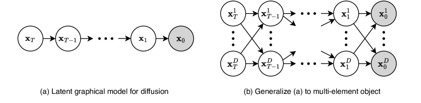
Figure 1: The graphical model diagram for both element-wise diffusion and multi-element diffusion.

7.2 Definition of nominal data

Nominal data, or categorical data, refers to data that can be categorized but not ranked or ordered. In mathematics, nominal data can be represented as a set of discrete categories or distinct labels without inherent ordering. As there is no ordering inside, operations of comparing categories is meaningless except checking equality. In the real world, most categories of data are nominal in nature, such as nationality, blood type, colors, among others.

7.3 Derivation of $q(x_{t-1}|x_{t},x_{0})$

First, let us define $\overline{Q}_{t|s}=Q_{s+1}...Q_{t}$. Note that $\overline{Q}_{t|0}=\overline{Q}_{t}$ and $\overline{Q}_{t|t-1}=Q_{t}$. Accordingly, we can derive the following two equalities.

$$q({\mathbf{x}}_{t}|{\mathbf{x}}_{s})=\text{Cat}({\mathbf{x}}_{t};\overline{Q}_{t|s}^{\top}{\mathbf{x}}_{s})\;$$ (35)

$$q({\mathbf{x}}_{s}|{\mathbf{x}}_{t},{\mathbf{x}}_{0}) =\frac{q({\mathbf{x}}_{t}|{\mathbf{x}}_{s})q({\mathbf{x}}_{s}|{\mathbf{x}}_{0})}{q({\mathbf{x}}_{t}|{\mathbf{x}}_{0})}=\frac{\text{Cat}({\mathbf{x}}_{t};\overline{Q}^{\top}_{t|s}{\mathbf{x}}_{s})\text{Cat}({\mathbf{x}}_{s};\overline{Q}_{s}^{\top}{\mathbf{x}}_{0})}{\text{Cat}({\mathbf{x}}_{t};\overline{Q}_{t}^{\top}{\mathbf{x}}_{0})}$$

$$=\frac{{\mathbf{x}}_{s}^{\top}\overline{Q}_{t|s}{\mathbf{x}}_{t}\cdot{\mathbf{x}}_{s}^{\top}\overline{Q}_{s}^{\top}{\mathbf{x}}_{0}}{{\mathbf{x}}_{t}^{\top}\overline{Q}_{t}^{\top}{\mathbf{x}}_{0}}={\mathbf{x}}_{s}^{\top}\frac{\overline{Q}_{t|s}{\mathbf{x}}_{t}\odot\overline{Q}_{s}^{\top}{\mathbf{x}}_{0}}{{\mathbf{x}}_{t}^{\top}\overline{Q}_{t}^{\top}{\mathbf{x}}_{0}}=\text{Cat}({\mathbf{x}}_{s};\frac{\overline{Q}_{t|s}{\mathbf{x}}_{t}\odot\overline{Q}_{s}^{\top}{\mathbf{x}}_{0}}{{\mathbf{x}}_{t}^{\top}\overline{Q}_{t}^{\top}{\mathbf{x}}_{0}})$$ (36)

Using the formulation of $Q_{t}$ in Eq. (7), $\overline{Q}_{t|s}$ can be written as

$$\overline{Q}_{t|s}=\overline{\alpha}_{t|s}I+(1-\overline{\alpha}_{t|s})\bm{1}{\bm{m}}^{\top}\;$$ (37)

where $\overline{\alpha}_{t|s}=\prod_{i=s+1}^{t}\alpha_{i}$. Note that $\overline{\alpha}_{t}=\overline{\alpha}_{t|s}\overline{\alpha}_{s}$.

Next, we can simplify Eq. (5) using the above formulations as

$$\frac{\overline{Q}_{t|s}{\mathbf{x}}_{t}\odot\overline{Q}_{s}^{\top}{\mathbf{x}}_{0}}{{\mathbf{x}}_{t}^{\top}\overline{Q}_{t}^{\top}{\mathbf{x}}_{0}}=\frac{\big{(}\overline{\alpha}_{t|s}{\mathbf{x}}_{t}+(1-\overline{\alpha}_{t|s})\langle{\bm{m}},{\mathbf{x}}_{t}\rangle\bm{1}\big{)}\odot\big{(}\overline{\alpha}_{s}{\mathbf{x}}_{0}+(1-\overline{\alpha}_{s}){\bm{m}}\big{)}}{\overline{\alpha}_{t}\langle{\mathbf{x}}_{t},{\mathbf{x}}_{0}\rangle+(1-\overline{\alpha}_{t})\langle{\bm{m}},{\mathbf{x}}_{t}\rangle}$$

$$=\frac{\overline{\alpha}_{t}{\mathbf{x}}_{t}\odot{\mathbf{x}}_{0}+(\overline{\alpha}_{s}-\overline{\alpha}_{t})\langle{\bm{m}},{\mathbf{x}}_{t}\rangle{\mathbf{x}}_{0}+(\overline{\alpha}_{t|s}-\overline{\alpha}_{t}){\mathbf{x}}_{t}\odot{\bm{m}}+(1-\overline{\alpha}_{s})(1-\overline{\alpha}_{t|s})\langle{\bm{m}},{\mathbf{x}}_{t}\rangle{\bm{m}}}{\overline{\alpha}_{t}\langle{\mathbf{x}}_{t},{\mathbf{x}}_{0}\rangle+(1-\overline{\alpha}_{t})\langle{\bm{m}},{\mathbf{x}}_{t}\rangle}$$ (38)

We can simplify the above equation further by considering two cases: (1) ${\mathbf{x}}_{t}={\mathbf{x}}_{0}$ and (2) ${\mathbf{x}}_{t}\neq{\mathbf{x}}_{0}$.

(Case 1) When ${\mathbf{x}}_{t}={\mathbf{x}}_{0}$, using the fact that both ${\mathbf{x}}_{t}$ and ${\mathbf{x}}_{0}$ are one-hot encoded, we observe

Eq. (38) $$=\frac{\overline{\alpha}_{t}{\mathbf{x}}_{t}+(\overline{\alpha}_{s}-\overline{\alpha}_{t})\langle{\bm{m}},{\mathbf{x}}_{t}\rangle{\mathbf{x}}_{t}+(\overline{\alpha}_{t|s}-\overline{\alpha}_{t})\langle{\bm{m}},{\mathbf{x}}_{t}\rangle{\mathbf{x}}_{t}+(1-\overline{\alpha}_{s})(1-\overline{\alpha}_{t|s})\langle{\bm{m}},{\mathbf{x}}_{t}\rangle{\bm{m}}}{\overline{\alpha}_{t}+(1-\overline{\alpha}_{t})\langle{\bm{m}},{\mathbf{x}}_{t}\rangle}$$

$$=\frac{\overline{\alpha}_{t}+(\overline{\alpha}_{t|s}+\overline{\alpha}_{s}-2\overline{\alpha}_{t})\langle{\bm{m}},{\mathbf{x}}_{t}\rangle}{\overline{\alpha}_{t}+(1-\overline{\alpha}_{t})\langle{\bm{m}},{\mathbf{x}}_{t}\rangle}{\mathbf{x}}_{t}+\frac{(1-\overline{\alpha}_{s})(1-\overline{\alpha}_{t|s})\langle{\bm{m}},{\mathbf{x}}_{t}\rangle}{\overline{\alpha}_{t}+(1-\overline{\alpha}_{t})\langle{\bm{m}},{\mathbf{x}}_{t}\rangle}{\bm{m}}$$

$$=(1-\lambda_{t|s})\cdot{\mathbf{x}}_{t}+\lambda_{t|s}\cdot{\bm{m}}\;,$$ (39)

where $\lambda_{t|s}$ is defined as

$$\lambda_{t|s}=\frac{(1-\overline{\alpha}_{s})(1-\overline{\alpha}_{t|s})\langle{\bm{m}},{\mathbf{x}}_{t}\rangle}{\overline{\alpha}_{t}+(1-\overline{\alpha}_{t})\langle{\bm{m}},{\mathbf{x}}_{t}\rangle}\;.$$ (40)

(Case 2) When ${\mathbf{x}}_{t}\neq{\mathbf{x}}_{0}$, we can similarly derive

Eq. (38) $$=\frac{(\overline{\alpha}_{s}-\overline{\alpha}_{t})\langle{\bm{m}},{\mathbf{x}}_{t}\rangle{\mathbf{x}}_{0}+(\overline{\alpha}_{t|s}-\overline{\alpha}_{t})\langle{\bm{m}},{\mathbf{x}}_{t}\rangle{\mathbf{x}}_{t}+(1-\overline{\alpha}_{s})(1-\overline{\alpha}_{t|s})\langle{\bm{m}},{\mathbf{x}}_{t}\rangle{\bm{m}}}{(1-\overline{\alpha}_{t})\langle{\bm{m}},{\mathbf{x}}_{t}\rangle}$$

$$=\frac{\overline{\alpha}_{s}-\overline{\alpha}_{t}}{1-\overline{\alpha}_{t}}{\mathbf{x}}_{0}+\frac{1-\overline{\alpha}_{s}}{1-\overline{\alpha}_{t}}\overline{\alpha}_{t|s}{\mathbf{x}}_{t}+\frac{1-\overline{\alpha}_{s}}{1-\overline{\alpha}_{t}}(1-\overline{\alpha}_{t|s}){\bm{m}}$$

$$=(1-\mu_{t|s})\cdot{\mathbf{x}}_{0}+\mu_{t|s}\overline{\alpha}_{t|s}\cdot{\mathbf{x}}_{t}+\mu_{t|s}(1-\overline{\alpha}_{t|s})\cdot{\bm{m}}\;,$$ (41)

where $\mu_{t|s}$ is defined as

$$\mu_{t|s}=\frac{1-\overline{\alpha}_{s}}{1-\overline{\alpha}_{t}}\;$$ (42)

Combining the results from both cases together, we can write $q({\mathbf{x}}_{s}|{\mathbf{x}}_{t},{\mathbf{x}}_{0})$ in the following form.

$$q({\mathbf{x}}_{s}|{\mathbf{x}}_{t},{\mathbf{x}}_{0})=\begin{cases}\text{Cat}\Big{(}{\mathbf{x}}_{s};\ (1-\lambda_{t|s})\cdot{\mathbf{x}}_{t}+\lambda_{t|s}\cdot{\bm{m}}\Big{)}&\text{when }{\mathbf{x}}_{t}={\mathbf{x}}_{0}\\ \text{Cat}\Big{(}{\mathbf{x}}_{s};\ (1-\mu_{t|s})\cdot{\mathbf{x}}_{0}+\mu_{t|s}\overline{\alpha}_{t|s}\cdot{\mathbf{x}}_{t}+\mu_{t|s}(1-\overline{\alpha}_{t|s})\cdot{\bm{m}}\Big{)}&\text{when }{\mathbf{x}}_{t}\neq{\mathbf{x}}_{0}\end{cases}$$ (43)

7.4 Parameterization of $p_{\theta}(x_{s}|x_{t})$

We first provide the formulation as follows.

$$p_{\theta}({\mathbf{x}}_{s}|{\mathbf{x}}_{t})=\sum_{{\mathbf{x}}_{0}}q({\mathbf{x}}_{s}|{\mathbf{x}}_{t},{\mathbf{x}}_{0})p_{\theta}({\mathbf{x}}_{0}|{\mathbf{x}}_{t})$$ (44)

Using $q({\mathbf{x}}_{s}|{\mathbf{x}}_{t},{\mathbf{x}}_{0})$ in Eq. (9) and $p_{\theta}({\mathbf{x}}_{0}|{\mathbf{x}}_{t})=\text{Cat}({\mathbf{x}}_{0};f_{t}^{\theta}({\mathbf{x}}_{t}))$, we can expand it as

$$p_{\theta}({\mathbf{x}}_{s}|{\mathbf{x}}_{t}) =q({\mathbf{x}}_{s}|{\mathbf{x}}_{t},{\mathbf{x}}_{t})p_{\theta}({\mathbf{x}}_{t}|{\mathbf{x}}_{t})+\sum_{{\mathbf{x}}\neq{\mathbf{x}}_{t}}q({\mathbf{x}}_{s}|{\mathbf{x}}_{t},{\mathbf{x}})p_{\theta}({\mathbf{x}}|{\mathbf{x}}_{t})$$

$$= {\mathbf{x}}_{s}^{\top}\Big{(}(1-\lambda_{t|s}){\mathbf{x}}_{t}+\lambda_{t|s}{\bm{m}}\Big{)}{\mathbf{x}}_{t}^{\top}f_{t}^{\theta}({\mathbf{x}}_{t})$$

$$+\sum_{{\mathbf{x}}\neq{\mathbf{x}}_{t}}{\mathbf{x}}_{s}^{T}\Big{(}(1-\mu_{t|s}){\mathbf{x}}+\mu_{t|s}\overline{\alpha}_{t|s}{\mathbf{x}}_{t}+\mu_{t|s}(1-\overline{\alpha}_{t|s}){\bm{m}}\Big{)}{\mathbf{x}}^{\top}f_{t}^{\theta}({\mathbf{x}}_{t})$$

$$= {\mathbf{x}}_{s}^{\top}\Big{[}\big{(}(1-\lambda_{t|s}){\mathbf{x}}_{t}+\lambda_{t|s}{\bm{m}}\big{)}{\mathbf{x}}_{t}^{\top}f_{t}^{\theta}({\mathbf{x}}_{t})+(1-\mu_{t|s})(\sum_{{\mathbf{x}}\neq{\mathbf{x}}_{t}}{\mathbf{x}}{\mathbf{x}}^{\top})f_{t}^{\theta}({\mathbf{x}}_{t})$$

$$+(\mu_{t|s}\overline{\alpha}_{t|s}{\mathbf{x}}_{t}+\mu_{t|s}(1-\overline{\alpha}_{t|s}){\bm{m}})(\sum_{{\mathbf{x}}\neq{\mathbf{x}}_{t}}{\mathbf{x}})^{\top}f_{t}^{\theta}({\mathbf{x}}_{t})\Big{]}$$

$$= {\mathbf{x}}_{s}^{\top}\Big{[}\big{(}(1-\lambda_{t|s}){\mathbf{x}}_{t}+\lambda_{t|s}{\bm{m}}\big{)}{\mathbf{x}}_{t}^{\top}f_{t}^{\theta}({\mathbf{x}}_{t})+(1-\mu_{t|s})(I-{\mathbf{x}}_{t}{\mathbf{x}}_{t}^{\top})f_{t}^{\theta}({\mathbf{x}}_{t})$$

$$+(\mu_{t|s}\overline{\alpha}_{t|s}{\mathbf{x}}_{t}+\mu_{t|s}(1-\overline{\alpha}_{t|s}){\bm{m}})(\bm{1}-{\mathbf{x}}_{t})^{\top}f_{t}^{\theta}({\mathbf{x}}_{t})\Big{]}$$

$$= {\mathbf{x}}_{s}^{\top}\Big{[}(1-\lambda_{t|s}){\mathbf{x}}_{t}^{\top}f_{t}^{\theta}({\mathbf{x}}_{t}){\mathbf{x}}_{t}+\lambda_{t|s}{\mathbf{x}}_{t}^{\top}f_{t}^{\theta}({\mathbf{x}}_{t}){\bm{m}}+(1-\mu_{t|s})(f_{t}^{\theta}({\mathbf{x}}_{t})-{\mathbf{x}}_{t}^{\top}f_{t}^{\theta}({\mathbf{x}}_{t}){\mathbf{x}}_{t})$$

$$+(\mu_{t|s}\overline{\alpha}_{t|s}{\mathbf{x}}_{t}+\mu_{t|s}(1-\overline{\alpha}_{t|s}){\bm{m}})(1-{\mathbf{x}}_{t}^{T}f_{t}^{\theta}({\mathbf{x}}_{t}))\Big{]}$$

$$= {\mathbf{x}}_{s}^{\top}\Big{[}(1-\mu_{t|s})\cdot f_{t}^{\theta}({\mathbf{x}}_{t})+\Big{(}(\mu_{t|s}-\lambda_{t|s}-\mu_{t|s}\overline{\alpha}_{t|s}){\mathbf{x}}_{t}^{\top}f_{t}^{\theta}({\mathbf{x}}_{t})+\mu_{t|s}\overline{\alpha}_{t|s}\Big{)}\cdot{\mathbf{x}}_{t}$$

$$+\Big{(}-(\mu_{t|s}-\lambda_{t|s}-\mu_{t|s}\overline{\alpha}_{t|s}){\mathbf{x}}_{t}^{\top}f_{t}^{\theta}({\mathbf{x}}_{t})+\mu_{t|s}(1-\overline{\alpha}_{t|s})\Big{)}\cdot{\bm{m}}\Big{]}$$

$$= \quad\text{Cat}\Big{(}{\mathbf{x}}_{s};\ (1-\mu_{t|s})\cdot f_{t}^{\theta}({\mathbf{x}}_{t})+(\mu_{t|s}\overline{\alpha}_{t|s}+\gamma^{\theta}_{{t|s}})\cdot{\mathbf{x}}_{t}+(\mu_{t|s}(1-\overline{\alpha}_{t|s})-\gamma^{\theta}_{{t|s}})\cdot{\bm{m}}\Big{)}$$ (45)

7.5 Proof of Proposition 3

As $q({\mathbf{x}}_{s}|{\mathbf{x}}_{t},{\mathbf{x}}_{0})$ has two different categorical distributions based on whether ${\mathbf{x}}_{t}$ is equal to ${\mathbf{x}}_{0}$, we prove the Proposition 3 based on two cases.

Case 1: ${\mathbf{x}}_{t}={\mathbf{x}}_{0}$. In this case, let $h^{\theta}_{t}:=f_{t}^{\theta}({\bm{x}}_{t})-{\bm{x}}_{0}$, now replace $f_{t}^{\theta}$ with $g_{t}^{\theta}$ in Eq. (12) and Eq. (11), we get

$$\gamma_{t|s}^{\theta}=(\mu_{t|s}-\lambda_{t|s}-\mu_{t|s}\overline{\alpha}_{t|s})\langle h^{\theta}_{t}+{\bm{x}}_{0},{\bm{x}}_{t}\rangle=(\mu_{t|s}-\lambda_{t|s}-\mu_{t|s}\overline{\alpha}_{t|s})\langle h^{\theta}_{t},{\bm{x}}_{t}\rangle+(\mu_{t|s}-\lambda_{t|s}-\mu_{t|s}\overline{\alpha}_{t|s})$$ (46)

Taking the formulation into Eq. (11) and cancel out terms, we can simplify $p_{\theta}({\mathbf{x}}_{s}|{\mathbf{x}}_{t})$ as

$$p_{\theta}({\mathbf{x}}_{s}|{\mathbf{x}}_{t}) =(1-\mu_{t|s})h^{\theta}_{t}+(1-\lambda_{t|s}){\bm{x}}_{t}+\lambda_{t|s}{\bm{m}}+(\mu_{t|s}-\lambda_{t|s}-\mu_{t|s}\overline{\alpha}_{t|s})\langle h^{\theta}_{t},{\bm{x}}_{t}\rangle({\bm{x}}_{t}-{\bm{m}})$$ (47)

$$=q({\mathbf{x}}_{s}|{\mathbf{x}}_{t},{\mathbf{x}}_{0})+(1-\mu_{t|s})\Big{[}h^{\theta}_{t}+\frac{\mu_{t|s}-\lambda_{t|s}-\mu_{t|s}\overline{\alpha}_{t|s}}{1-\mu_{t|s}}\langle h^{\theta}_{t},{\bm{x}}_{t}\rangle({\bm{x}}_{t}-{\bm{m}})\Big{]}$$ (48)

$$=q({\mathbf{x}}_{s}|{\mathbf{x}}_{t},{\mathbf{x}}_{0})+(1-\mu_{t|s})\Big{[}h^{\theta}_{t}+\phi_{t|s}\langle h^{\theta}_{t},{\bm{x}}_{t}\rangle({\bm{x}}_{t}-{\bm{m}})\Big{]}$$ (49)

Case 2: ${\mathbf{x}}_{t}\neq{\mathbf{x}}_{0}$. Based on Eq. (9) and Eq. (11), it’s easy to find that

$$p_{\theta}({\mathbf{x}}_{s}|{\mathbf{x}}_{t}) =(1-\mu_{t|s})(f^{\theta}_{t}({\bm{x}}_{t})-{\bm{x}}_{0})+\gamma_{t|s}^{\theta}({\bm{x}}_{t}-{\bm{m}})+(1-\mu_{t|s}){\bm{x}}_{0}+\mu_{t|s}\bar{\alpha}_{t|s}{\bm{x}}_{t}+\mu_{t|s}(1-\bar{\alpha}_{t|s}){\bm{m}}$$ (50)

$$=(1-\mu_{t|s})(f^{\theta}_{t}({\bm{x}}_{t})-{\bm{x}}_{0})+\gamma_{t|s}^{\theta}({\bm{x}}_{t}-{\bm{m}})+q({\mathbf{x}}_{s}|{\mathbf{x}}_{t},{\mathbf{x}}_{0})$$ (51)

$$=q({\mathbf{x}}_{s}|{\mathbf{x}}_{t},{\mathbf{x}}_{0})+(1-\mu_{t|s})\Big{[}f^{\theta}_{t}({\bm{x}}_{t})-{\bm{x}}_{0}+\frac{\gamma_{t|s}^{\theta}}{(1-\mu_{t|s})}({\bm{x}}_{t}-{\bm{m}})\Big{]}$$ (52)

Taking the definition of $\gamma_{t|s}^{\theta}$ in Eq. (12) and using the fact $<{\bm{x}}_{0},{\bm{x}}_{t}>=0$ we get the formulation in proposition 3.

For both cases, we proved that the formulation in proposition 3 is correct.

7.6 Proof of KL divergence approximation

Assume that $p({\bm{x}})=q({\bm{x}})+\triangle p({\bm{x}})$, and both $p({\bm{x}})$ and $q({\bm{x}})$ are valid categorical distributions. Then

$$D_{\mathrm{KL}}\big{(}q({\bm{x}})\|p({\bm{x}})\big{)} =-\sum_{\bm{x}}q({\bm{x}})\log\frac{p({\bm{x}})}{q({\bm{x}})}=-\sum_{\bm{x}}q({\bm{x}})\log(1+\frac{\triangle p({\bm{x}})}{q({\bm{x}})})$$ (53)

By Taylor expansion, $\log(1+x)\approx x-\frac{x^{2}}{2}$, we ignore larger than 2 order terms. Then apply this we get

$$D_{\mathrm{KL}}\big{(}q({\bm{x}})\|p({\bm{x}})\big{)} =-\sum_{\bm{x}}q({\bm{x}})[\frac{\triangle p({\bm{x}})}{q({\bm{x}})}-(\frac{\triangle p({\bm{x}})}{q({\bm{x}})})^{2}]$$ (54)

$$=-\sum_{\bm{x}}\triangle p({\bm{x}})+\sum_{\bm{x}}\frac{\triangle p({\bm{x}})^{2}}{q({\bm{x}})}$$ (55)

$$=\sum_{\bm{x}}\frac{\triangle p({\bm{x}})^{2}}{q({\bm{x}})}$$ (56)

Change probabilities $q$ and $p$ to $q_{(}{\mathbf{x}}_{s}|{\mathbf{x}}_{t},{\mathbf{x}}_{0})$ and $p_{\theta}({\mathbf{x}}_{s}|{\mathbf{x}}_{t})$ we get the targeted formulation.

7.7 VLB with partial time steps

Assume that we only observe ${\mathbf{x}}_{t}$, ${\mathbf{x}}_{s}$, and ${\mathbf{x}}_{0}$, and assume that we have learned the prior $p_{\theta}({\mathbf{x}}_{t})$.

$$\log p_{\theta}({\mathbf{x}}_{0}) =\log\mathbb{E}_{q({\mathbf{x}}_{t},{\mathbf{x}}_{s}|{\mathbf{x}}_{0})}\frac{p_{\theta}({\mathbf{x}}_{t},{\mathbf{x}}_{s},{\mathbf{x}}_{0})}{q({\mathbf{x}}_{t},{\mathbf{x}}_{s}|{\mathbf{x}}_{0})}\geq\mathbb{E}_{q({\mathbf{x}}_{t},{\mathbf{x}}_{s}|{\mathbf{x}}_{0})}\log\frac{p_{\theta}({\mathbf{x}}_{t},{\mathbf{x}}_{s},{\mathbf{x}}_{0})}{q({\mathbf{x}}_{t},{\mathbf{x}}_{s}|{\mathbf{x}}_{0})}$$ (57)

$$=\mathbb{E}_{q({\mathbf{x}}_{t},{\mathbf{x}}_{s}|{\mathbf{x}}_{0})}[\log\frac{p_{\theta}({\mathbf{x}}_{t})p_{\theta}({\mathbf{x}}_{s}|{\mathbf{x}}_{t})p_{\theta}({\mathbf{x}}_{0}|{\mathbf{x}}_{s})}{q({\mathbf{x}}_{t}|{\mathbf{x}}_{0})q({\mathbf{x}}_{s}|{\mathbf{x}}_{t},{\mathbf{x}}_{0})}]$$ (58)

$$=\mathbb{E}_{q({\mathbf{x}}_{t},{\mathbf{x}}_{s}|{\mathbf{x}}_{0})}\Big{[}\log\frac{p_{\theta}({\mathbf{x}}_{t})}{q({\mathbf{x}}_{t}|{\mathbf{x}}_{0})}+\log p_{\theta}({\mathbf{x}}_{t})+\log\frac{p_{\theta}({\mathbf{x}}_{s}|{\mathbf{x}}_{t})}{q({\mathbf{x}}_{s}|{\mathbf{x}}_{t},{\mathbf{x}}_{0})}\Big{]}$$ (59)

$$=-D_{\mathrm{KL}}[q({\mathbf{x}}_{t}|{\mathbf{x}}_{0})\|p_{\theta}({\mathbf{x}}_{t})]+\mathbb{E}_{q({\mathbf{x}}_{s}|{\mathbf{x}}_{0})}\log p_{\theta}({\mathbf{x}}_{0}|{\mathbf{x}}_{s})-D_{\mathrm{KL}}[q({\mathbf{x}}_{s}|{\mathbf{x}}_{t},{\mathbf{x}}_{0})\|p_{\theta}({\mathbf{x}}_{s}|{\mathbf{x}}_{t})]$$ (60)

7.8 Discrete-Time Multi-element Object Extension

We first extend $q({\mathbf{x}}_{t}|{\mathbf{x}}_{0})$, $q({\mathbf{x}}_{s}|{\mathbf{x}}_{t},{\mathbf{x}}_{0})$, and $p_{\theta}({\mathbf{x}}_{s}|{\mathbf{x}}_{t})$ to multi-element object, and then present the negative VLB loss extension. First, for the forward process conditional on ${\mathbf{x}}_{0}$, each element ${\mathbf{x}}^{d}_{t}$ of the multi-element object ${\mathbf{x}}^{1:D}_{t}$ has its own diffusion process without interactions with others. Formally,

$$q({\mathbf{x}}_{t}^{1:D}|{\mathbf{x}}_{0}^{1:D})=\prod_{d=1}^{D}q({\mathbf{x}}_{t}^{d}|{\mathbf{x}}_{0}^{d})\quad,\text{and}\quad q({\mathbf{x}}^{1:D}_{s}|{\mathbf{x}}^{1:D}_{t},{\mathbf{x}}^{1:D}_{0})=\prod_{d=1}^{D}q({\mathbf{x}}^{d}_{s}|{\mathbf{x}}^{d}_{t},{\mathbf{x}}^{d}_{0})\;.$$ (61)

The corresponding forward reparameterization form for generating ${\mathbf{x}}^{1:D}_{t|0}$ can be updated as

$${\mathbf{x}}^{1:D}_{t|0} =\delta^{1:D}_{1,{\mathbf{b}}^{1:D}_{t}}\odot{\mathbf{x}}^{1:D}_{0}+(1-\delta^{1:D}_{1,{\mathbf{b}}^{1:D}_{t}})\odot{\mathbf{m}}^{1:D}_{0}\quad,$$ (62)

where $\delta^{1:D}_{1,{\mathbf{b}}^{1:D}_{t}}$ is a $D$-dimensional vector with $d$-th element being $\delta_{1,{\mathbf{b}}^{d}_{t}}$ and ${\mathbf{b}}^{d}_{t}\sim\text{Bernoulli}(\overline{\alpha}_{t})$.

For the backward process, all elements’ transition processes are coupled together, as shown in the graphical model in Appx. Fig. 1(b). We start with the parameterization $p_{\theta}({\mathbf{x}}^{1:D}_{0}|{\mathbf{x}}^{1:D}_{t})$, with the form

$$p_{\theta}({\mathbf{x}}^{1:D}_{0}|{\mathbf{x}}^{1:D}_{t})=\prod_{d=1}^{D}p_{\theta}({\mathbf{x}}^{d}_{0}|{\mathbf{x}}^{1:D}_{t})\quad\text{with}\quad p_{\theta}({\mathbf{x}}^{d}_{0}|{\mathbf{x}}^{1:D}_{t})=\text{Cat}\big{(}{\mathbf{x}}_{0}^{d}|f_{t}^{\theta,d}({\mathbf{x}}_{t}^{1:D})\big{)}$$ (63)

Then, $p_{\theta}({\mathbf{x}}^{1:D}_{s}|{\mathbf{x}}^{1:D}_{t})=\prod_{d=1}^{D}p_{\theta}({\mathbf{x}}^{d}_{s}|{\mathbf{x}}^{1:D}_{t})$, with the component $p_{\theta}({\mathbf{x}}^{d}_{s}|{\mathbf{x}}^{1:D}_{t})$ has the form

$$\text{Cat}\Big{(}{\mathbf{x}}^{d}_{s};\ (1-\mu_{t|s})f_{t}^{\theta,d}({\mathbf{x}}_{t}^{1:D})+(\mu_{t|s}\overline{\alpha}_{t|s}+\gamma^{\theta,d}_{{t|s}}){\mathbf{x}}_{t}^{d}+(\mu_{t|s}(1-\overline{\alpha}_{t|s})-\gamma^{\theta,d}_{{t|s}}){\bm{m}}^{d}\Big{)}\;,$$ (64)

$$\text{where }\gamma^{\theta,d}_{{t|s}}=(\mu_{t|s}-\lambda^{d}_{t|s}-\mu_{t|s}\overline{\alpha}_{t|s})\langle f_{t}^{\theta,d}({\mathbf{x}}_{t}^{1:D}),{\mathbf{x}}^{d}_{t}\rangle,\ \lambda^{d}_{t|s}=\frac{(1-\overline{\alpha}_{s})(1-\overline{\alpha}_{t|s})\langle{\bm{m}}^{d},{\mathbf{x}}^{d}_{t}\rangle}{\overline{\alpha}_{t}+(1-\overline{\alpha}_{t})\langle{\bm{m}}^{d},{\mathbf{x}}^{d}_{t}\rangle}\;.$$

Similarly, the reparameterization form can be expressed as

$${\mathbf{x}}_{s|t}^{1:D}=\delta^{1:D}_{1,{\mathbf{b}}^{1:D}_{s|t}}\odot\tilde{{\mathbf{x}}}^{1:D}_{0|t}\;+\;\delta^{1:D}_{2,{\mathbf{b}}^{1:D}_{s|t}}\odot{\mathbf{x}}_{t}^{1:D}\;+\;\delta^{1:D}_{3,{\mathbf{b}}^{1:D}_{s|t}}\odot{\mathbf{m}}_{0}^{1:D}\;,$$ (65)

where $\tilde{{\mathbf{x}}}^{d}_{0|t}\sim\text{Cat}(f_{t}^{\theta,d}({\mathbf{x}}_{t}^{1:D}))$ and ${\mathbf{b}}^{d}_{s|t}\sim\text{Cat}(1-\mu_{t|s},\ \mu_{t|s}\overline{\alpha}_{t|s}+\gamma^{\theta,d}_{{t|s}},\ \mu_{t|s}(1-\overline{\alpha}_{t|s})-\gamma^{\theta,d}_{{t|s}})$.

Finally, the following reformulate the loss functions $\mathcal{L}_{t}(\theta)$ for multi-element objects, where we drop the constant term for simplicity.

$$\mathcal{L}^{1:D}_{t}(\theta)= \mathbb{E}_{q({\mathbf{x}}^{1:D}_{t}|{\mathbf{x}}^{1:D}_{0})}\sum_{d=1}^{D}\Big{[}\delta_{{\mathbf{x}}^{d}_{t},{\mathbf{x}}^{d}_{0}}\mathbb{E}_{q({\mathbf{x}}^{d}_{t-1}|{\mathbf{x}}^{d}_{t}={\mathbf{x}}^{d}_{0})}[-\log p_{\theta}({\mathbf{x}}^{d}_{t-1}|{\mathbf{x}}^{1:D}_{t})]+$$

$$\qquad\qquad\qquad(1-\delta_{{\mathbf{x}}^{d}_{t},{\mathbf{x}}^{d}_{0}})\mathbb{E}_{q({\mathbf{x}}^{d}_{t-1}|{\mathbf{x}}^{d}_{t}\neq{\mathbf{x}}^{d}_{0})}[-\log p_{\theta}({\mathbf{x}}^{d}_{t-1}|{\mathbf{x}}^{1:D}_{t})]\Big{]}$$ (66)

7.9 CTMC introduction

The CTMC process can go with either increasing $t$ or decreasing $t$, and we use increasing $t$ as the default direction to introduce CTMC. For any CTMC, its transition rate matrix $R_{t}$ with $[R_{t}]_{ij}=r_{t}({\bm{e}}_{j}|{\bm{e}}_{i})$ fully determines the underlying stochastic process. CTMC is categorized into time-homogeneous and time-inhomogeneous based on whether $R_{t}$ is static with respect to $t$. In this paper we work with time-inhomogeneous CTMC.

Based on the definition in Eq. (23), we can derive some properties as follows

$$\forall{\bm{x}},r_{t}({\bm{x}}|{\bm{x}})\leq 0;\qquad\forall{\bm{y}}\neq{\bm{x}},r_{t}({\bm{y}}|{\bm{x}})\geq 0;\qquad\forall{\bm{x}},\sum_{{\bm{y}}}r_{t}({\bm{y}}|{\bm{x}})=0$$ (67)

$$q_{t|t-\triangle t}({\bm{y}}|{\bm{x}})=\delta_{{\bm{x}},{\bm{y}}}+r_{t}({\bm{y}}|{\bm{x}})\triangle t+o(\triangle t)$$ (68)

Eq. (67) shows the properties of transition rate, which imply $r_{t}({\bm{x}}|{\bm{x}})=-\sum_{{\bm{y}}\neq{\bm{x}}}r_{t}({\bm{y}}|{\bm{x}})$. Eq. (68) characterizes the infinitesimal change of transition probability, and can be used to derive the relationship between transition matrix $\overline{Q}_{t|s}$ and transition rate matrix $R_{t}$. Formally, a CTMC’s transition probabilities satisfies the Kolmogorov forward and backward equations (Kolmogoroff, 1931) :

$$\frac{d}{dt}q_{t|s}({\bm{y}}|{\bm{x}})=\sum_{{\mathbf{z}}}q_{t|s}({\bm{z}}|{\bm{x}})r_{t}({\bm{y}}|{\bm{z}})\quad \text{or}\quad\frac{d}{dt}\overline{Q}_{t|s}=\overline{Q}_{t|s}R_{t}$$ Kolmogorov Forward (69)

$$\frac{d}{ds}q_{t|s}({\bm{y}}|{\bm{x}})=-\sum_{{\bm{z}}}r_{s}({\bm{z}}|{\bm{x}})q_{t|s}({\bm{y}}|{\bm{z}})\quad \text{or}\quad\frac{d}{ds}\overline{Q}_{t|s}=-R_{s}\overline{Q}_{t|s}$$ Kolmogorov Backward (70)

The above equations are Ordinary Different Equations (ODEs) and have unique solutions. (Rindos et al., 1995) mentioned that when $R_{t_{1}}$ and $R_{t_{2}}$ commute (i.e. $R_{t_{1}}R_{t_{2}}=R_{t_{2}}R_{t_{1}}$) for any $t_{1},t_{2}$, the transition probability matrix can be written as

$$\overline{Q}_{t|s}=\exp\Big{(}\int_{s}^{t}R_{a}da\Big{)}\;$$ (71)

where $\exp(M):=\sum_{k=0}^{\infty}\frac{M^{k}}{k!}$ is the matrix exponential operation. The commutative property of $R_{t}$ can be achieved by choosing $R_{t}=\beta(t)R_{b}$ where $R_{b}\in\mathbb{R}^{K\times K}$ is a time-independent base transition rate matrix satisfying properties in Eq. (67) and $\beta(t)$ is a positive scalar dependent on time. Now assume $R_{b}$ is diagonalizable and $R_{b}=U\Sigma U^{-1}$ by eigen-decomposition, then we can simplify Eq. (24) as

$$\overline{Q}_{t|s}=\exp\Big{(}\int_{s}^{t}\beta(t)R_{b}da\Big{)}=\exp(\overline{\beta}_{t|s}R_{b})=\exp(\overline{\beta}_{t|s}U\Sigma U^{-1})=U\exp(\overline{\beta}_{t|s}\Sigma)U^{-1}$$ (72)

where $\overline{\beta}_{t|s}:=\int_{s}^{t}\beta(a)da$.

7.10 Derivation of Eq. (25)

$$\overline{Q}_{t|s}=\exp(\overline{\beta}_{t|s}R_{b}) =I+\sum_{k=1}^{\infty}\frac{(-\overline{\beta}_{t|s})^{k}(-R_{b})^{k}}{k!}=I-(\sum_{k=1}^{\infty}\frac{(-\overline{\beta}_{t|s})^{k}}{k!})R_{b}$$

$$=I-(e^{-\overline{\beta}_{t|s}}-1)R_{b}=e^{-\overline{\beta}_{t|s}}I+(1-e^{-\overline{\beta}_{t|s}})\bm{1}{\bm{m}}^{\top}$$ (73)

7.11 Derivation of Eq. (32)

With the help of Eq. (26), we first show that $g_{t}^{\theta}$ can be simplified as follows.

$$g^{\theta}_{t}({\bm{z}}|{\bm{x}}) =\frac{1}{\langle{\bm{x}},{\bm{m}}\rangle}\Big{[}\langle{\bm{z}},{\bm{m}}\rangle+\frac{\overline{\alpha}_{t|0}}{1-\overline{\alpha}_{t|0}}p^{\theta}_{0|t}({\bm{z}}|{\bm{x}})-\frac{\overline{\alpha}_{t|0}\langle{\bm{z}},{\bm{m}}\rangle}{\overline{\alpha}_{t|0}+(1-\overline{\alpha}_{t|0})\langle{\bm{x}},{\bm{m}}\rangle}p^{\theta}_{0|t}({\bm{x}}|{\bm{x}})\Big{]}$$

$$=\frac{1}{\langle{\bm{x}},{\bm{m}}\rangle}\Big{[}\big{(}1-\frac{\overline{\alpha}_{t|0}p^{\theta}_{0|t}({\bm{x}}|{\bm{x}})}{\overline{\alpha}_{t|0}+(1-\overline{\alpha}_{t|0})\langle{\bm{x}},{\bm{m}}\rangle}\big{)}\langle{\bm{z}},{\bm{m}}\rangle+\frac{\overline{\alpha}_{t|0}}{1-\overline{\alpha}_{t|0}}p^{\theta}_{0|t}({\bm{z}}|{\bm{x}})\Big{]}\quad\forall{\bm{z}}\neq{\bm{x}}$$ (74)

Proof.

$$\frac{q_{t|0}({\bm{z}}|{\bm{x}}_{0})}{q_{t|0}({\bm{x}}|{\bm{x}}_{0})}=\frac{{\bm{z}}^{\top}\overline{Q}_{t|0}^{\top}{\bm{x}}_{0}}{{\bm{x}}^{\top}\overline{Q}_{t|0}^{\top}{\bm{x}}_{0}}=\frac{\overline{\alpha}_{t|0}{\bm{z}}^{\top}{\bm{x}}_{0}+(1-\overline{\alpha}_{t|0})\langle{\bm{z}},{\bm{m}}\rangle}{\overline{\alpha}_{t|0}{\bm{x}}^{\top}{\bm{x}}_{0}+(1-\overline{\alpha}_{t|0})\langle{\bm{x}},{\bm{m}}\rangle}$$ (75)

Then when ${\bm{z}}\neq{\bm{x}}$, we can write it as

$$\frac{q_{t|0}({\bm{z}}|{\bm{x}}_{0})}{q_{t|0}({\bm{x}}|{\bm{x}}_{0})}=\begin{cases}\frac{\langle{\bm{z}},{\bm{m}}\rangle}{\langle{\bm{x}},{\bm{m}}\rangle}&\quad\text{if }{\bm{x}}_{0}\neq{\bm{x}}\text{ and }{\bm{x}}_{0}\neq{\bm{z}}\\[5.0pt] \frac{\frac{\overline{\alpha}_{t|0}}{1-\overline{\alpha}_{t|0}}+\langle{\bm{z}},{\bm{m}}\rangle}{\langle{\bm{x}},{\bm{m}}\rangle}&\quad\text{if }{\bm{x}}_{0}={\bm{z}}\\[5.0pt] \frac{\langle{\bm{z}},{\bm{m}}\rangle}{\frac{\overline{\alpha}_{t|0}}{1-\overline{\alpha}_{t|0}}+\langle{\bm{x}},{\bm{m}}\rangle}&\quad\text{if }{\bm{x}}_{0}={\bm{x}}\end{cases}$$ (76)

Hence,

$$g^{\theta}_{t}({\bm{z}}|{\bm{x}})=\sum_{{\bm{x}}_{0}}\frac{q_{t|0}({\bm{z}}|{\bm{x}}_{0})}{q_{t|0}({\bm{x}}|{\bm{x}}_{0})}p_{0|t}^{\theta}({\bm{x}}_{0}|{\bm{x}})$$

$$=\frac{q_{t|0}({\bm{z}}|{\bm{x}})}{q_{t|0}({\bm{x}}|{\bm{x}})}p_{0|t}^{\theta}({\bm{x}}|{\bm{x}})+\frac{q_{t|0}({\bm{z}}|{\bm{z}})}{q_{t|0}({\bm{x}}|{\bm{z}})}p_{0|t}^{\theta}({\bm{z}}|{\bm{x}})+\sum_{{\bm{x}}_{0}\neq{\bm{z}},{\bm{x}}}\frac{q_{t|0}({\bm{z}}|{\bm{x}}_{0})}{q_{t|0}({\bm{x}}|{\bm{x}}_{0})}p_{0|t}^{\theta}({\bm{x}}_{0}|{\bm{x}})$$

$$=\frac{\langle{\bm{z}},{\bm{m}}\rangle}{\frac{\overline{\alpha}_{t|0}}{1-\overline{\alpha}_{t|0}}+\langle{\bm{x}},{\bm{m}}\rangle}p^{\theta}_{0|t}({\bm{x}}|{\bm{x}})+\frac{\frac{\overline{\alpha}_{t|0}}{1-\overline{\alpha}_{t|0}}+\langle{\bm{z}},{\bm{m}}\rangle}{\langle{\bm{x}},{\bm{m}}\rangle}p^{\theta}_{0|t}({\bm{z}}|{\bm{x}})+\frac{\langle{\bm{z}},{\bm{m}}\rangle}{\langle{\bm{x}},{\bm{m}}\rangle}(1-p^{\theta}_{0|t}({\bm{z}}|{\bm{x}})-p^{\theta}_{0|t}({\bm{x}}|{\bm{x}}))$$

$$=\frac{1}{\langle{\bm{x}},{\bm{m}}\rangle}\Big{[}\big{(}1-\frac{\overline{\alpha}_{t|0}p^{\theta}_{0|t}({\bm{x}}|{\bm{x}})}{\overline{\alpha}_{t|0}+(1-\overline{\alpha}_{t|0})\langle{\bm{x}},{\bm{m}}\rangle}\big{)}\langle{\bm{z}},{\bm{m}}\rangle+\frac{\overline{\alpha}_{t|0}}{1-\overline{\alpha}_{t|0}}p^{\theta}_{0|t}({\bm{z}}|{\bm{x}})\Big{]}\quad\forall{\bm{z}}\neq{\bm{x}}$$ (77)

Additionally, when ${\bm{z}}={\bm{x}}$, $g_{t}^{\theta}({\bm{z}}|{\bm{x}})=\sum_{{\bm{x}}_{0}}p^{\theta}_{0|t}({\bm{x}}_{0}|{\bm{x}})=1$. ∎

We can also compute the vectorization $g_{t}^{\theta}(\cdot|{\bm{x}})$ directly as

$$g_{t}^{\theta}(\cdot|{\bm{x}})=\frac{1}{\langle{\bm{x}},{\bm{m}}\rangle}\Big{[}\big{(}1-\frac{\overline{\alpha}_{t|0}\langle f_{t}^{\theta}({\bm{x}}),{\bm{x}}\rangle}{\overline{\alpha}_{t|0}+(1-\overline{\alpha}_{t|0})\langle{\bm{x}},{\bm{m}}\rangle}\big{)}{\bm{m}}+\frac{\overline{\alpha}_{t|0}}{1-\overline{\alpha}_{t|0}}f_{t}^{\theta}({\bm{x}})\Big{]}\odot(\bm{1}-{\bm{x}})+{\bm{x}}$$ (78)

where $f_{t}^{\theta}({\bm{x}})$ is the parameterized neural network for $p^{\theta}_{0|t}(\cdot|{\bm{x}})$ that outputs the distribution of ${\mathbf{x}}_{0|t}$. Eq. (32) combines Eq. (74) and $g_{t}^{\theta}({\bm{x}}|{\bm{x}})=1,\forall{\bm{x}}$.

7.12 Derivation of Forward and Backward Transition Rate in Multi-element Case

In this section, we show how to extend transition rates, and and the ratio $g_{t}^{\theta}$, into multi-element case. We let ${\bm{x}}^{\backslash d}$ represent ${\bm{x}}^{1:D\backslash d}$, i.e. the object without $d$-th element, for simplicity.

Forward Transition Rates: First, the transition rates for forward sampling has a specific decomposition formulation in multi-element case as proven by (Campbell et al., 2022), thus, we summarize the result as follows. The key assumption for CTMC is that at a single time, only one dimension can change.

$$r^{1:D}_{t}({\bm{y}}^{1:D}|{\bm{x}}^{1:D})=\sum_{d=1}^{D}r^{d}_{t}({\bm{y}}^{d}|{\bm{x}}^{d})\delta_{{\bm{x}}^{\backslash d},{\bm{y}}^{\backslash d}}$$ (79)

where $\delta_{{\bm{x}}^{\backslash d},{\bm{y}}^{\backslash d}}$ is the Kronecker delta and it is 1 if and only if ${\bm{x}}^{\backslash d}={\bm{y}}^{\backslash d}$. As we also assume that all dimension processes are indepedent, $r^{d}_{t}$ denotes the transition rate of the CTMC process at d-th element/dimension.

Backward Transition Rates: Now let us work on $\hat{r}_{t}^{1:D}({\bm{y}}^{1:D}|{\bm{x}}^{1:D})$. Notice that as the backward process is also a CTMC, it also satisfies that only one dimension can change at a time. We summarize two equivalent formulations as follows.

$$\hat{r}^{1:D}_{t}({\bm{y}}^{1:D}|{\bm{x}}^{1:D}) =\sum_{d=1}^{D}r^{d}_{t}({\bm{x}}^{d}|{\bm{y}}^{d})\delta_{{\bm{x}}^{\backslash d},{\bm{y}}^{\backslash d}}\sum_{{\bm{x}}_{0}^{d}}\frac{q_{t|0}({\bm{y}}^{d}|{{\bm{x}}_{0}^{d}})}{q_{t|0}({\bm{x}}^{d}|{{\bm{x}}_{0}^{d}})}q_{0|t}({\bm{x}}_{0}^{d}|{\bm{x}}^{1:D})$$ (80)

$$\hat{r}^{1:D}_{t}({\bm{y}}^{1:D}|{\bm{x}}^{1:D}) =\sum_{d=1}^{D}\frac{r^{d}_{t}({\bm{x}}^{d}|{\bm{y}}^{d})\delta_{{\bm{x}}^{\backslash d},{\bm{y}}^{\backslash d}}}{\sum_{{\bm{x}}_{0}^{d}}\frac{q_{t|0}({\bm{x}}^{d}|{{\bm{x}}_{0}^{d}})}{q_{t|0}({\bm{y}}^{d}|{{\bm{x}}_{0}^{d}})}q_{0|t}({\bm{x}}_{0}^{d}|{\bm{y}}^{1:D})}$$ (81)

Notice that these two formulations should be equivalent. In practice, we use the first formulation to parameterize the reverse transition rate in learning.

Proof.

$$\frac{q_{t}({\bm{y}}^{1:D})}{q_{t}({\bm{x}}^{1:D})}=\sum_{{\bm{x}}_{0}^{1:D}}\frac{q_{t|0}({\bm{y}}^{1:D}|{\bm{x}}_{0}^{1:D})}{q_{t|0}({\bm{x}}^{1:D}|{\bm{x}}_{0}^{1:D})}q_{0|t}({\bm{x}}_{0}^{1:D}|{\bm{x}}^{1:D})=\sum_{{\bm{x}}_{0}^{1:D}}q_{0|t}({\bm{x}}_{0}^{1:D}|{\bm{x}}^{1:D})\prod_{d=1}^{D}\frac{q_{t|0}({\bm{y}}^{d}|{\bm{x}}_{0}^{d})}{q_{t|0}({\bm{x}}^{d}|{\bm{x}}_{0}^{d})}$$ (82)

$$\sum_{{\bm{x}}_{0}^{\backslash d}}q_{0|t}({{\bm{x}}_{0}^{1:D}}|{\bm{x}}^{1:D})=\sum_{{\bm{x}}_{0}^{\backslash d}}q_{0|t}({{\bm{x}}_{0}^{d}}|{\bm{x}}^{1:D})q_{0|t}({{\bm{x}}_{0}^{\backslash d}}|{\bm{x}}^{1:D},{\bm{x}}_{0}^{d})=q_{0|t}({{\bm{x}}_{0}^{d}}|{\bm{x}}^{1:D})$$ (83)

(Case 1)

$$\hat{r}^{1:D}_{t}({\bm{y}}^{1:D}|{\bm{x}}^{1:D}) =r^{1:D}_{t}({\bm{x}}^{1:D}|{\bm{y}}^{1:D})\frac{q_{t}({\bm{y}}^{1:D})}{q_{t}({\bm{x}}^{1:D})}$$

$$=\Big{(}\sum_{d=1}^{D}r^{d}_{t}({\bm{x}}^{d}|{\bm{y}}^{d})\delta_{{\bm{x}}^{\backslash d},{\bm{y}}^{\backslash d}}\Big{)}\Big{(}\sum_{{\bm{x}}_{0}^{1:D}}q_{0|t}({\bm{x}}_{0}^{1:D}|{\bm{x}}^{1:D})\prod_{d=1}^{D}\frac{q_{t|0}({\bm{y}}^{d}|{\bm{x}}_{0}^{d})}{q_{t|0}({\bm{x}}^{d}|{\bm{x}}_{0}^{d})}\Big{)}$$

$$=\sum_{d=1}^{D}\sum_{\color[rgb]{0,0,0}{\bm{x}}_{0}^{1:D}}r^{d}_{t}({\bm{x}}^{d}|{\bm{y}}^{d})\delta_{{\bm{x}}^{\backslash d},{\bm{y}}^{\backslash d}}q_{0|t}({\color[rgb]{0,0,0}{\bm{x}}_{0}^{1:D}}|{\bm{x}}^{1:D})\frac{q_{t|0}({\bm{y}}^{d}|{\color[rgb]{0,0,0}{\bm{x}}_{0}^{d}})}{q_{t|0}({\bm{x}}^{d}|{\color[rgb]{0,0,0}{\bm{x}}_{0}^{d}})}$$

$$=\sum_{d=1}^{D}r^{d}_{t}({\bm{x}}^{d}|{\bm{y}}^{d})\delta_{{\bm{x}}^{\backslash d},{\bm{y}}^{\backslash d}}\sum_{\color[rgb]{0,0,0}{\bm{x}}_{0}^{d}}\frac{q_{t|0}({\bm{y}}^{d}|{\color[rgb]{0,0,0}{\bm{x}}_{0}^{d}})}{q_{t|0}({\bm{x}}^{d}|{\color[rgb]{0,0,0}{\bm{x}}_{0}^{d}})}\sum_{{\bm{x}}_{0}^{\backslash d}}q_{0|t}({{\bm{x}}_{0}^{1:D}}|{\bm{x}}^{1:D})$$

$$=\sum_{d=1}^{D}r^{d}_{t}({\bm{x}}^{d}|{\bm{y}}^{d})\delta_{{\bm{x}}^{\backslash d},{\bm{y}}^{\backslash d}}\sum_{{\bm{x}}_{0}^{d}}\frac{q_{t|0}({\bm{y}}^{d}|{{\bm{x}}_{0}^{d}})}{q_{t|0}({\bm{x}}^{d}|{{\bm{x}}_{0}^{d}})}q_{0|t}({\bm{x}}_{0}^{d}|{\bm{x}}^{1:D})$$ (84)

(Case 2)

$$\hat{r}^{1:D}_{t}({\bm{y}}^{1:D}|{\bm{x}}^{1:D}) =r^{1:D}_{t}({\bm{x}}^{1:D}|{\bm{y}}^{1:D})/\frac{q_{t}({\bm{x}}^{1:D})}{q_{t}({\bm{y}}^{1:D})}$$

$$=\sum_{d=1}^{D}\frac{r^{d}_{t}({\bm{x}}^{d}|{\bm{y}}^{d})\delta_{{\bm{x}}^{\backslash d},{\bm{y}}^{\backslash d}}}{\sum_{{\bm{x}}_{0}^{1:D}}q_{0|t}({\bm{x}}_{0}^{1:D}|{\bm{y}}^{1:D})\prod_{i=1}^{D}\frac{q_{t|0}({\bm{x}}^{i}|{\bm{x}}_{0}^{i})}{q_{t|0}({\bm{y}}^{i}|{\bm{x}}_{0}^{i})}}$$

$$=\sum_{d=1}^{D}\frac{r^{d}_{t}({\bm{x}}^{d}|{\bm{y}}^{d})\delta_{{\bm{x}}^{\backslash d},{\bm{y}}^{\backslash d}}}{\sum_{{\bm{x}}_{0}^{1:D}}q_{0|t}({\bm{x}}_{0}^{1:D}|{\bm{y}}^{1:D})\frac{q_{t|0}({\bm{x}}^{d}|{\bm{x}}_{0}^{d})}{q_{t|0}({\bm{y}}^{d}|{\bm{x}}_{0}^{d})}}$$

$$=\sum_{d=1}^{D}\frac{r^{d}_{t}({\bm{x}}^{d}|{\bm{y}}^{d})\delta_{{\bm{x}}^{\backslash d},{\bm{y}}^{\backslash d}}}{\sum_{{\bm{x}}_{0}^{d}}\frac{q_{t|0}({\bm{x}}^{d}|{{\bm{x}}_{0}^{d}})}{q_{t|0}({\bm{y}}^{d}|{{\bm{x}}_{0}^{d}})}q_{0|t}({\bm{x}}_{0}^{d}|{\bm{y}}^{1:D})}$$ (85)

∎

Ratio: We now define an estimator $g_{t}^{\theta,d}({\bm{x}}^{d}|{\bm{y}}^{1:D})$ as follows.

$$g_{t}^{\theta,d}({\bm{x}}^{d}|{\bm{y}}^{1:D}): =\sum_{{\bm{x}}_{0}^{d}}\frac{q_{t|0}({\bm{x}}^{d}|{\bm{x}}_{0}^{d})}{q_{t|0}({\bm{y}}^{d}|{\bm{x}}_{0}^{d})}p_{0|t}^{\theta}({\bm{x}}_{0}^{d}|{\bm{y}}^{1:D})\approx\sum_{{\bm{x}}_{0}^{d}}\frac{q_{t|0}({\bm{x}}^{d}|{\bm{x}}_{0}^{d})}{q_{t|0}({\bm{y}}^{d}|{\bm{x}}_{0}^{d})}q_{0|t}({\bm{x}}_{0}^{d}|{\bm{y}}^{1:D})=\frac{q_{t}({\bm{x}}^{d}|{\bm{y}}^{\backslash d})}{q_{t}({\bm{y}}^{d}|{\bm{y}}^{\backslash d})}$$ (86)

$$g_{t}^{\theta}({\bm{x}}^{1:D}|{\bm{y}}^{1:D}): =\prod_{d=1}^{D}g^{\theta,d}_{t}({\bm{x}}^{d}|{\bm{y}}^{1:D})=\sum_{{\bm{x}}_{0}^{1:D}}\frac{q_{t|0}({\bm{x}}^{1:D}|{\bm{x}}_{0}^{1:D})}{q_{t|0}({\bm{y}}^{1:D}|{\bm{x}}_{0}^{1:D})}p_{0|t}^{\theta}({\bm{x}}_{0}^{1:D}|{\bm{y}}^{1:D})\approx\frac{q_{t}({\bm{x}}^{1:D})}{q_{t}({\bm{y}}^{1:D})}$$ (87)

We can extend the vector formulation Eq. (32) in Proposition 4 to $g_{t}^{\theta,d}({\bm{x}}^{d}|{\bm{y}}^{1:D})$:

$$g_{t}^{\theta,d}(\cdot|{\bm{x}}^{1:D})=\frac{1}{\langle{\bm{x}}^{d},{\bm{m}}^{d}\rangle}\Big{[}\big{(}1-\frac{\overline{\alpha}_{t|0}\langle f_{t}^{\theta,d}({\bm{x}}^{1:D}),{\bm{x}}^{d}\rangle}{\overline{\alpha}_{t|0}+(1-\overline{\alpha}_{t|0})\langle{\bm{x}}^{d},{\bm{m}}^{d}\rangle}\big{)}{\bm{m}}^{d}+\frac{\overline{\alpha}_{t|0}}{1-\overline{\alpha}_{t|0}}f_{t}^{\theta,d}({\bm{x}}^{1:D})\Big{]}\odot(\bm{1}-{\bm{x}}^{d})+{\bm{x}}^{d}$$ (88)

Then, we can derive two approximators for transition rate $\hat{r}^{1:D}_{t}({\bm{y}}^{1:D}|{\bm{x}}^{1:D})$ as follows.

$$[\hat{r}^{\theta,1:D}_{t}]^{1}({\bm{y}}^{1:D}|{\bm{x}}^{1:D}) :=\sum_{d=1}^{D}r^{d}_{t}({\bm{x}}^{d}|{\bm{y}}^{d})g_{t}^{\theta,d}({\bm{y}}^{d}|{\bm{x}}^{1:D})\cdot\delta_{{\bm{x}}^{\backslash d},{\bm{y}}^{\backslash d}}\approx\text{Eq.~{}(\ref{eq:rate_multi_element_1})}$$ (89)

$$[\hat{r}^{\theta,1:D}_{t}]^{2}({\bm{y}}^{1:D}|{\bm{x}}^{1:D}) :=\sum_{d=1}^{D}\frac{r^{d}_{t}({\bm{x}}^{d}|{\bm{y}}^{d})}{g_{t}^{\theta,d}({\bm{x}}^{d}|{\bm{y}}^{1:D})}\cdot\delta_{{\bm{x}}^{\backslash d},{\bm{y}}^{\backslash d}}\approx\text{Eq.~{}(\ref{eq:rate_multi_element_2})}$$ (90)

7.13 Derivation of Negative VLB Loss in Multi-element Case

As forward process is defined in Eq. (26), in multi-element case we can easily get

$$r^{d}_{t}({\bm{x}}^{d}|\cdot) =R^{d}_{t}{\bm{x}}^{d}=\beta(t)\big{(}\langle{\bm{x}}^{d},{\bm{m}}^{d}\rangle\bm{1}-{\bm{x}}^{d}\big{)}$$ (91)

$$r^{d}_{t}(\cdot|{\bm{x}}^{d}) =(R^{d}_{t})^{\top}{\bm{x}}^{d}=\beta(t)\big{(}{\bm{m}}^{d}-{\bm{x}}^{d}\big{)}$$ (92)

The $r^{d}_{t}({\bm{x}}|\cdot)$ and $r^{d}_{t}(\cdot|{\bm{x}})$ are essentially the ${\bm{x}}$-th column and row of the transition rate matrix $R^{d}_{t}$.

In Mult-element case, the negative VLB loss in Eq. (30) can be written as

$$T\ \mathbb{E}_{\begin{subarray}{c}t\sim\text{Uni}(0,T)\\ {\bm{x}}^{1:D}\sim q_{t|0}\end{subarray}}\Big{[}\sum_{{\bm{z}}^{1:D}\neq{\bm{x}}^{1:D}}\hat{r}_{t}^{\theta,1:D}({\bm{z}}^{1:D}|{\bm{x}}^{1:D})-\sum_{{\bm{z}}^{1:D}\neq{\bm{x}}^{1:D}}r^{1:D}_{t}({\bm{z}}^{1:D}|{\bm{x}}^{1:D})\log\hat{r}_{t}^{\theta,1:D}({\bm{x}}^{1:D}|{\bm{z}}^{1:D})\Big{]}$$ (93)

As there are two terms, let’s work on each term separately.

7.13.1 Term 1

Based on the formulation of $r_{t}^{1:D}$ and $\hat{r}_{t}^{\theta,1:D}$, we can rewrite the first term as

Term1 $$=T\ \mathbb{E}_{t,{\bm{x}}^{1:D}}\sum_{{\bm{z}}^{1:D}\neq{\bm{x}}^{1:D}}\hat{r}_{t}^{\theta,1:D}({\bm{z}}^{1:D}|{\bm{x}}^{1:D})$$ (94)

$$=T\ \mathbb{E}_{t,{\bm{x}}^{1:D}}\sum_{{\bm{z}}^{1:D}\neq{\bm{x}}^{1:D}}\sum_{d=1}^{D}r^{d}_{t}({\bm{x}}^{d}|{\bm{z}}^{d})g_{t}^{\theta,d}({\bm{z}}^{d}|{\bm{x}}^{1:D})\cdot\delta_{{\bm{x}}^{\backslash d},{\bm{z}}^{\backslash d}}$$ (95)

$$=T\ \mathbb{E}_{t,{\bm{x}}^{1:D}}\Big{[}\sum_{d=1}^{D}\sum_{{\bm{z}}^{d}\neq{\bm{x}}^{d}}r^{d}_{t}({\bm{x}}^{d}|{\bm{z}}^{d})g_{t}^{\theta,d}({\bm{z}}^{d}|{\bm{x}}^{1:D})\Big{]}$$ (96)

$$=T\ \mathbb{E}_{t,{\bm{x}}^{1:D}}\Big{[}\sum_{d=1}^{D}r^{d}_{t}({\bm{x}}^{d}|\cdot)^{\top}g_{t}^{\theta,d}(\cdot|{\bm{x}}^{1:D})\Big{]}+\text{const.}$$ (97)

$$=T\ \mathbb{E}_{\begin{subarray}{c}t\sim\text{Uni.}(0,T)\\ {\bm{x}}^{1:D}\sim q_{t|0}\end{subarray}}\ \beta(t)\sum_{d=1}^{D}\langle{\bm{x}}^{d},{\bm{m}}^{d}\rangle\Big{[}\bm{1}^{\top}g_{t}^{\theta,d}(\cdot|{\bm{x}}^{1:D})\Big{]}+\text{const.}$$ (98)

7.13.2 Term 2

As the evaluation of $\hat{r}^{\theta}_{t}(\cdot|{\bm{x}})$ for any ${\bm{x}}$ requires a single forward pass of the parameterized network $p_{0|t}^{\theta}(\cdot|{\bm{x}})$, the second term within the expectation of Eq. (30) requires multiple passes of the model. This complexity is even greatly amplified in cases with multi-element objects. Campbell et al. (2022) avoids the multiple passes by changing the expectation variable through importance sampling. We take a similar approach to simplify the second term. Differently, Campbell et al. (2022) uses a specific sampling distribution (same as the forward transition rate) to introduce the auxiliary variable for changing the expectation variable, we generalize it to use a general sampling process $S_{t}$ defined below.

Let ${\bm{y}}^{1:D}$ be the new variable upon which the exchanged expectation is based, and assume that ${\bm{y}}^{1:D}$ is sampled from an unnormalized joint distribution $S_{t}({\bm{y}}^{1:D}|{\bm{x}}^{1:D})$. We restrict $S_{t}({\bm{y}}^{1:D}|{\bm{x}}^{1:D})$ to be a unnormalized probability that is nonzero if and only if ${\bm{y}}^{1:D}$ and ${\bm{x}}^{1:D}$ are different at a single element. Formally, we can write the unnormalized distribution as

$$S_{t}({\bm{y}}^{1:D}|{\bm{x}}^{1:D}) =(1-\delta_{{\bm{y}}^{1:D},{\bm{x}}^{1:D}})\sum_{d=1}^{D}S^{d}_{t}({\bm{y}}^{d}|{\bm{x}}^{d})\delta_{{\bm{y}}^{\backslash d},{\bm{x}}^{\backslash d}}$$

$$\text{with normalizer }{\mathcal{S}}_{t}({\bm{x}}^{1:D}) =\sum_{{\bm{y}}^{1:D}}S_{t}({\bm{y}}^{1:D}|{\bm{x}}^{1:D})=\sum_{d=1}^{D}\sum_{{\bm{y}}^{d}\neq{\bm{x}}^{d}}S_{t}^{d}({\bm{y}}^{d}|{\bm{x}}^{d})$$ (99)

where $S_{t}^{d}({\bm{y}}^{d}|{\bm{x}}^{d})$ is any unnormalized probability at dimension $d$.

Now for the second term, we have

Term2 $$=T\ \mathbb{E}_{t,{\bm{x}}^{1:D}}\sum_{{\bm{z}}^{1:D}\neq{\bm{x}}^{1:D}}r_{t}({\bm{z}}^{1:D}|{\bm{x}}^{1:D})\log\hat{r}_{t}^{\theta}({\bm{x}}^{1:D}|{\bm{z}}^{1:D})$$ (100)

$$=T\ \mathbb{E}_{t,{\bm{x}}^{1:D}}\sum_{{\bm{z}}^{1:D}\neq{\bm{x}}^{1:D}}\frac{S_{t}({\bm{z}}^{1:D}|{\bm{x}}^{1:D})}{{\mathcal{S}}({\bm{x}}^{1:D})}\cdot\frac{{\mathcal{S}}_{t}({\bm{x}}^{1:D})}{S_{t}({\bm{z}}^{1:D}|{\bm{x}}^{1:D})}\cdot r_{t}({\bm{z}}^{1:D}|{\bm{x}}^{1:D})\log\hat{r}_{t}^{\theta}({\bm{x}}^{1:D}|{\bm{z}}^{1:D})$$ (101)

$$=T\ \mathbb{E}_{\begin{subarray}{c}t,{\bm{x}}^{1:D}\\ {\bm{z}}^{1:D}\sim S_{t}\end{subarray}}\Big{[}\frac{{\mathcal{S}}_{t}({\bm{x}}^{1:D})}{S_{t}({\bm{z}}^{1:D}|{\bm{x}}^{1:D})}\cdot r_{t}({\bm{z}}^{1:D}|{\bm{x}}^{1:D})\log\hat{r}_{t}^{\theta}({\bm{x}}^{1:D}|{\bm{z}}^{1:D})\Big{]}\qquad\text{ (As $S_{t}$ samples ${\bm{z}}^{1:D}\neq{\bm{x}}^{1:D}$ )}$$ (102)

$$=T\ \mathbb{E}_{\begin{subarray}{c}t,{\bm{z}}^{1:D}\sim S_{t}\end{subarray}}\sum_{{\bm{x}}^{1:D}}\Big{[}q_{S_{t}}({\bm{x}}^{1:D}|{\bm{x}}_{0}^{1:D},{\bm{z}}^{1:D})\cdot\frac{{\mathcal{S}}_{t}({\bm{x}}^{1:D})}{S_{t}({\bm{z}}^{1:D}|{\bm{x}}^{1:D})}\cdot r_{t}({\bm{z}}^{1:D}|{\bm{x}}^{1:D})\log\hat{r}_{t}^{\theta}({\bm{x}}^{1:D}|{\bm{z}}^{1:D})\Big{]}$$ (103)

where $q_{S_{t}}({\bm{x}}^{1:D}|{\bm{x}}_{0}^{1:D},{\bm{z}}^{1:D})$ is the conditional posterior distribution such that (for clearity we replace ${\bm{x}}^{1:D},{\bm{z}}^{1:D}$ with ${\bm{x}}^{1:D}_{t},{\bm{z}}^{1:D}_{t}$ respectively, as they are variables at time $t$)

$$q_{S_{t}}({\bm{x}}_{t}^{1:D}|{\bm{x}}_{0}^{1:D},{\bm{z}}_{t}^{1:D}) =\frac{q_{S_{t}}({\bm{x}}_{t}^{1:D},{\bm{z}}_{t}^{1:D}|{\bm{x}}_{0}^{1:D})}{\sum_{{\bm{y}}_{t}^{1:D}}q_{S_{t}}({\bm{y}}_{t}^{1:D},{\bm{z}}_{t}^{1:D}|{\bm{x}}_{0}^{1:D})}=\frac{q_{t|0}({\bm{x}}^{1:D}_{t}|{\bm{x}}^{1:D}_{0})\cdot S_{t}({\bm{z}}^{1:D}_{t}|{\bm{x}}^{1:D}_{t})/{\mathcal{S}}_{t}({\bm{x}}^{1:D}_{t})}{\sum_{{\bm{y}}^{1:D}_{y}}q_{t|0}({\bm{x}}^{1:D}|{\bm{x}}^{1:D}_{0})\cdot S_{t}({\bm{z}}^{1:D}_{t}|{\bm{y}}^{1:D}_{t})/{\mathcal{S}}_{t}({\bm{y}}^{1:D}_{t})}$$ (104)

$$=\frac{(1-\delta_{{\bm{z}}_{t},{\bm{x}}_{t}})\sum_{d=1}^{D}\delta_{{\bm{z}}_{t}^{\backslash d},{\bm{x}}_{t}^{\backslash d}}S_{t}^{d}({\bm{z}}_{t}^{d}|{\bm{x}}_{t}^{d})/{\mathcal{S}}_{t}({\bm{x}}_{t}^{1:D})\cdot q_{t|0}({\bm{x}}^{d}_{t}\circ{\bm{z}}_{t}^{\backslash d}|{\bm{x}}_{0}^{1:D})}{\sum_{{\bm{y}}^{1:D}_{t}}\big{[}(1-\delta_{{\bm{z}}_{t},{\bm{y}}_{t}})\sum_{d=1}^{D}\delta_{{\bm{z}}_{t}^{\backslash d},{\bm{y}}_{t}^{\backslash d}}S_{t}^{d}({\bm{z}}_{t}^{d}|{\bm{y}}_{t}^{d})/{\mathcal{S}}_{t}({\bm{y}}_{t}^{1:D})\cdot q_{t|0}({\bm{y}}_{t}^{d}\circ{\bm{z}}_{t}^{\backslash d}|{\bm{x}}_{0}^{1:D})\big{]}}$$ (105)

$$=\frac{(1-\delta_{{\bm{z}}_{t},{\bm{x}}_{t}})\sum_{d=1}^{D}\delta_{{\bm{z}}_{t}^{\backslash d},{\bm{x}}_{t}^{\backslash d}}\frac{S_{t}^{d}({\bm{z}}_{t}^{d}|{\bm{x}}_{t}^{d})}{{\mathcal{S}}_{t}({\bm{x}}_{t}^{1:D})}\cdot\frac{q_{t|0}({\bm{x}}^{d}_{t}|{\bm{x}}_{0}^{d})}{q_{t|0}({\bm{z}}^{d}_{t}|{\bm{x}}_{0}^{d})}}{\sum_{{\bm{y}}_{t}^{1:D}}\big{[}(1-\delta_{{\bm{z}}_{t},{\bm{y}}_{t}})\sum_{d=1}^{D}\delta_{{\bm{z}}_{t}^{\backslash d},{\bm{y}}_{t}^{\backslash d}}\frac{S_{t}^{d}({\bm{z}}_{t}^{d}|{\bm{y}}_{t}^{d})}{{\mathcal{S}}_{t}({\bm{y}}_{t}^{1:D})}\cdot\frac{q_{t|0}({\bm{y}}_{t}^{d}|{\bm{x}}_{0}^{d})}{q_{t|0}({\bm{z}}^{d}_{t}|{\bm{x}}_{0}^{d})}\big{]}}$$ (106)

$$=\frac{(1-\delta_{{\bm{z}}_{t},{\bm{x}}_{t}})\sum_{d=1}^{D}\delta_{{\bm{z}}_{t}^{\backslash d},{\bm{x}}_{t}^{\backslash d}}\frac{S_{t}^{d}({\bm{z}}_{t}^{d}|{\bm{x}}_{t}^{d})}{{\mathcal{S}}_{t}({\bm{x}}_{t}^{1:D})}\cdot\frac{q_{t|0}({\bm{x}}^{d}_{t}|{\bm{x}}_{0}^{d})}{q_{t|0}({\bm{z}}^{d}_{t}|{\bm{x}}_{0}^{d})}}{\sum_{d=1}^{D}\sum_{{\bm{y}}_{t}^{d}\neq{\bm{z}}^{d}}\frac{S_{t}^{d}({\bm{z}}_{t}^{d}|{\bm{y}}_{t}^{d})}{{\mathcal{S}}_{t}({\bm{y}}_{t}^{d}\circ{\bm{z}}_{t}^{\backslash d})}\cdot\frac{q_{t|0}({\bm{y}}_{t}^{d}|{\bm{x}}_{0}^{d})}{q_{t|0}({\bm{z}}^{d}_{t}|{\bm{x}}_{0}^{d})}}$$ (107)

Now taking the formulation of $q_{S_{t}}$ back into Term 2, we further simplify Term 2 as

Term2 $$=T\ \mathbb{E}_{\begin{subarray}{c}t,{\bm{z}}^{1:D}\sim S_{t}\end{subarray}}\frac{\sum_{{\bm{x}}^{1:D}}\Big{[}(1-\delta_{{\bm{z}},{\bm{x}}})\sum_{d=1}^{D}\delta_{{\bm{z}}^{\backslash d},{\bm{x}}^{\backslash d}}\frac{S_{t}^{d}({\bm{z}}^{d}|{\bm{x}}^{d})}{S_{t}({\bm{z}}^{1:D}|{\bm{x}}^{1:D})}\cdot\frac{q_{t|0}({\bm{x}}^{d}|{\bm{x}}_{0}^{d})}{q_{t|0}({\bm{z}}^{d}|{\bm{x}}_{0}^{d})}\cdot r_{t}({\bm{z}}^{1:D}|{\bm{x}}^{1:D})\log\hat{r}_{t}^{\theta}({\bm{x}}^{1:D}|{\bm{z}}^{1:D})\Big{]}}{\sum_{d=1}^{D}\sum_{{\bm{y}}^{d}\neq{\bm{z}}^{d}}\frac{S_{t}^{d}({\bm{z}}^{d}|{\bm{y}}^{d})}{{\mathcal{S}}_{t}({\bm{y}}^{d}\circ{\bm{z}}^{\backslash d})}\cdot\frac{q_{t|0}({\bm{y}}^{d}|{\bm{x}}_{0}^{d})}{q_{t|0}({\bm{z}}^{d}|{\bm{x}}_{0}^{d})}}$$ (108)

$$=\mathbb{E}_{\begin{subarray}{c}t,{\bm{z}}^{1:D}\sim S_{t}\end{subarray}}\frac{\sum_{d=1}^{D}\sum_{{\bm{x}}^{d}\neq{\bm{z}}^{d}}\frac{S_{t}^{d}({\bm{z}}^{d}|{\bm{x}}^{d})}{S_{t}({\bm{z}}^{1:D}|{\bm{x}}^{d}\circ{\bm{z}}^{\backslash d})}\cdot\frac{q_{t|0}({\bm{x}}^{d}|{\bm{x}}_{0}^{d})}{q_{t|0}({\bm{z}}^{d}|{\bm{x}}_{0}^{d})}\cdot r_{t}({\bm{z}}^{1:D}|{\bm{x}}^{d}\circ{\bm{z}}^{\backslash d})\log\hat{r}_{t}^{\theta}({\bm{x}}^{d}\circ{\bm{z}}^{\backslash d}|{\bm{z}}^{1:D})}{\sum_{d=1}^{D}\sum_{{\bm{y}}^{d}\neq{\bm{z}}^{d}}\frac{S_{t}^{d}({\bm{z}}^{d}|{\bm{y}}^{d})}{{\mathcal{S}}_{t}({\bm{y}}^{d}\circ{\bm{z}}^{\backslash d})}\cdot\frac{q_{t|0}({\bm{y}}^{d}|{\bm{x}}_{0}^{d})}{q_{t|0}({\bm{z}}^{d}|{\bm{x}}_{0}^{d})}}$$ (109)

$$=\mathbb{E}_{\begin{subarray}{c}t,{\bm{z}}^{1:D}\sim S_{t}\end{subarray}}\frac{\sum_{d=1}^{D}\sum_{{\bm{x}}^{d}\neq{\bm{z}}^{d}}\frac{q_{t|0}({\bm{x}}^{d}|{\bm{x}}_{0}^{d})}{q_{t|0}({\bm{z}}^{d}|{\bm{x}}_{0}^{d})}\cdot r_{t}^{d}({\bm{z}}^{d}|{\bm{x}}^{d})\cdot\log r^{d}_{t}({\bm{z}}^{d}|{\bm{x}}^{d})g_{t}^{\theta,d}({\bm{x}}^{d}|{\bm{z}}^{1:D})}{\sum_{d=1}^{D}\sum_{{\bm{y}}^{d}\neq{\bm{z}}^{d}}\frac{q_{t|0}({\bm{y}}^{d}|{\bm{x}}_{0}^{d})}{q_{t|0}({\bm{z}}^{d}|{\bm{x}}_{0}^{d})}\cdot\frac{S_{t}^{d}({\bm{z}}^{d}|{\bm{y}}^{d})}{{\mathcal{S}}_{t}({\bm{y}}^{d}\circ{\bm{z}}^{\backslash d})}}$$ (110)

$$=\mathbb{E}_{\begin{subarray}{c}t,{\bm{z}}^{1:D}\sim S_{t}\end{subarray}}\frac{\sum_{d=1}^{D}\sum_{{\bm{x}}^{d}\neq{\bm{z}}^{d}}\frac{q_{t|0}({\bm{x}}^{d}|{\bm{x}}_{0}^{d})}{q_{t|0}({\bm{z}}^{d}|{\bm{x}}_{0}^{d})}\cdot r_{t}^{d}({\bm{z}}^{d}|{\bm{x}}^{d})\cdot\log g_{t}^{\theta,d}({\bm{x}}^{d}|{\bm{z}}^{1:D})}{\sum_{d=1}^{D}\sum_{{\bm{y}}^{d}\neq{\bm{z}}^{d}}\frac{q_{t|0}({\bm{y}}^{d}|{\bm{x}}_{0}^{d})}{q_{t|0}({\bm{z}}^{d}|{\bm{x}}_{0}^{d})}\cdot\frac{S_{t}^{d}({\bm{z}}^{d}|{\bm{y}}^{d})}{{\mathcal{S}}_{t}({\bm{y}}^{d}\circ{\bm{z}}^{\backslash d})}}+\text{const.}$$ (111)

The above equation further shows that the sampling distribution $S_{t}$ for adding exchanging variable ${\bm{z}}^{1:D}$ only affect a weighting term of the loss computation. Let us define the scalar weighting term as

$${\mathcal{M}}_{S_{t}}({\bm{z}}^{1:D}|{\bm{x}}^{1:D}_{0}):=\sum_{d=1}^{D}\sum_{{\bm{y}}^{d}\neq{\bm{z}}^{d}}\frac{q_{t|0}({\bm{y}}^{d}|{\bm{x}}_{0}^{d})}{q_{t|0}({\bm{z}}^{d}|{\bm{x}}_{0}^{d})}\cdot\frac{S_{t}^{d}({\bm{z}}^{d}|{\bm{y}}^{d})}{{\mathcal{S}}_{t}({\bm{y}}^{d}\circ{\bm{z}}^{\backslash d})}$$ (112)

With this definition, the Term 2 can be further rewrited as

Term2 $$=\mathbb{E}_{\begin{subarray}{c}t,{\bm{z}}^{1:D}\sim S_{t}\end{subarray}}\Big{[}\frac{1}{{\mathcal{M}}_{S_{t}}({\bm{z}}^{1:D}|{\bm{x}}^{1:D}_{0})}\sum_{d=1}^{D}\frac{1}{q_{t|0}({\bm{z}}^{d}|{\bm{x}}_{0}^{d})}\sum_{{\bm{x}}^{d}\neq{\bm{z}}^{d}}q_{t|0}({\bm{x}}^{d}|{\bm{x}}_{0}^{d})\cdot r_{t}^{d}({\bm{z}}^{d}|{\bm{x}}^{d})\cdot\log g_{t}^{\theta,d}({\bm{x}}^{d}|{\bm{z}}^{1:D})\Big{]}$$ (113)

$$=\mathbb{E}_{\begin{subarray}{c}t,{\bm{z}}^{1:D}\sim S_{t}\end{subarray}}\Big{[}\frac{1}{{\mathcal{M}}_{S_{t}}({\bm{z}}^{1:D}|{\bm{x}}^{1:D}_{0})}\sum_{d=1}^{D}\frac{\bm{1}^{\top}[q_{t|0}(\cdot|{\bm{x}}_{0}^{d})\odot r_{t}^{d}({\bm{z}}^{d}|\cdot)\odot\log g_{t}^{\theta,d}(\cdot|{\bm{z}}^{1:D})]}{q_{t|0}({\bm{z}}^{d}|{\bm{x}}_{0}^{d})}\Big{]}+\text{const.}$$ (114)

$$=\mathbb{E}_{\begin{subarray}{c}t,{\bm{z}}^{1:D}\sim S_{t}\end{subarray}}\Big{[}\frac{\beta(t)}{{\mathcal{M}}_{S_{t}}({\bm{z}}^{1:D}|{\bm{x}}^{1:D}_{0})}\sum_{d=1}^{D}\frac{\langle{\bm{z}}^{d},{\bm{m}}^{d}\rangle}{q_{t|0}({\bm{z}}^{d}|{\bm{x}}_{0}^{d})}\bm{1}^{\top}[q_{t|0}(\cdot|{\bm{x}}_{0}^{d})\odot\log g_{t}^{\theta,d}(\cdot|{\bm{z}}^{1:D})]+\text{const.}\Big{]}$$ (115)

7.13.3 All Terms

Combine term 1 and term 2 together, we can write the negative VLB loss as

$$T\ \mathbb{E}_{\begin{subarray}{c}t\sim\text{Uni}(0,T)\\ {\bm{x}}^{1:D}\sim q_{t|0}\end{subarray}}\Big{[}\sum_{{\bm{z}}^{1:D}\neq{\bm{x}}^{1:D}}\hat{r}_{t}^{\theta,1:D}({\bm{z}}^{1:D}|{\bm{x}}^{1:D})-\sum_{{\bm{z}}^{1:D}\neq{\bm{x}}^{1:D}}r^{1:D}_{t}({\bm{z}}^{1:D}|{\bm{x}}^{1:D})\log\hat{r}_{t}^{\theta,1:D}({\bm{x}}^{1:D}|{\bm{z}}^{1:D})\Big{]}$$ (116)

$$=T\ \mathbb{E}_{\begin{subarray}{c}t\sim\text{Uni}(0,T)\\ {\bm{x}}^{1:D}\sim q_{t|0}({\bm{x}}_{0}^{1:D})\\ {\bm{z}}^{1:D}\sim S_{t}({\bm{x}}^{1:D})\end{subarray}}\Big{[}\sum_{d=1}^{D}r^{d}_{t}({\bm{x}}^{d}|\cdot)^{\top}g_{t}^{\theta,d}(\cdot|{\bm{x}}^{1:D})-\frac{1}{{\mathcal{M}}_{S_{t}}({\bm{z}}^{1:D}|{\bm{x}}^{1:D}_{0})}\sum_{d=1}^{D}\frac{\bm{1}^{\top}[q_{t|0}(\cdot|{\bm{x}}_{0}^{d})\odot r_{t}^{d}({\bm{z}}^{d}|\cdot)\odot\log g_{t}^{\theta,d}(\cdot|{\bm{z}}^{1:D})]}{q_{t|0}({\bm{z}}^{d}|{\bm{x}}_{0}^{d})}\Big{]}+\text{const.}$$ (117)

7.14 Algorithm for Unified Training and Generation

Alg. 1 and Alg. 2 demonstrate our unified training and generation framework.

Algorithm 1 USD3 Unified Training: Red: discrete-time step, and blue: continuous-time step.

1:  Input: A stationary distribution ${\bm{m}}$, samples $\sim p_{\text{data}}$, weight factor $\lambda$, max time $T$

2:  repeat

3:   Draw ${\mathbf{x}}_{0}\sim p_{\text{data}}({\mathbf{x}}_{0})$

4:   Draw $t\sim\textbf{Uniform}({0,...,T})$ or $t\sim\textbf{Uniform}(0,1)$

5:   Compute $\overline{\alpha}_{t}$ from Table 3

6:   Draw ${\mathbf{m}}_{0}^{1:D}\sim\text{Cat}({\mathbf{m}}_{0}^{1:D};{\bm{m}})$

7:   ${\mathbf{x}}^{1:D}_{t|0}=\delta^{1:D}_{1,{\mathbf{b}}^{1:D}_{t}}\odot{\mathbf{x}}^{1:D}_{0}+(1-\delta^{1:D}_{1,{\mathbf{b}}^{1:D}_{t}})\odot{\mathbf{m}}^{1:D}_{0}$ $\text{ where }{\mathbf{b}}_{t}\sim\text{Bernoulli}(\overline{\alpha}_{t})$, from Eq. (62)

8:   Compute $f_{t}^{\theta}({\bm{x}}_{t}^{1:D})$ as parameterization of $p_{\theta}({\mathbf{x}}_{0}^{1:D}|{\mathbf{x}}_{t}^{1:D})$

9:   Take gradient descent step on $\nabla_{\theta}\{\mathcal{L}_{t}(\theta)+\lambda\mathcal{L}^{CE}_{t}(\theta)\}$ (from Eq. (13) $+$ Eq. (14))

10:            or $\nabla_{\theta}\{\mathcal{L}^{CTMC}_{t}(\theta)+\lambda\mathcal{L}^{CE}_{t}(\theta)\}$ (from Eq. (30) $+$ Eq. (14))

11:  until convergence

Algorithm 2 USD3 Unified Sampling

1:  Input: A stationary distribution ${\bm{m}}$, $\{t_{i}\}_{i=0}^{n}$ s.t. $0=t_{0}<t_{1}<...<t_{n}=T$, learned $f^{\theta}_{t_{i}}$.

2:  MCMC Input: use$\_$MCMC, step size $\triangle n$, total steps $N$.

3:  Set ${\mathbf{x}}_{n}^{1:D}\sim\text{Cat}({\mathbf{x}}_{n}^{1:D};{\bm{m}})$

4:  for $i\in\{n,...,0\}$ do

5:   Compute $f_{t_{i}}^{\theta}({\bm{x}}_{i}^{1:D})$ and $p_{\theta}({\mathbf{x}}_{i-1}^{1:D}|{\mathbf{x}}_{i}^{1:D})$ from Eq. (11)

6:   Draw ${\mathbf{x}}_{i-1}^{1:D}\sim\text{Cat}({\mathbf{x}}_{i-1}^{1:D};p_{\theta}({\mathbf{x}}_{i-1}^{1:D}|{\mathbf{x}}_{i}^{1:D}))$

7:   If use$\_$MCMC:

8:    ${\mathbf{x}}_{i-1}^{1:D}\leftarrow\text{MCMC$\_$Corrector}(t_{i},{\mathbf{x}}_{i-1}^{1:D},\triangle n,f_{t_{i}}^{\theta},N)$ (Algo. 3)

9:  return ${\mathbf{x}}_{0}$

7.15 Continuous-Time MCMC Sampling Corrector & Noise Scheduling

7.15.1 The MCMC Sampling Corrector

(Song et al., 2021b) introduced a predictor-corrector step to further improve the quality of generated data based on score-based Markov Chain Monte Carlo (MCMC) for continuous-time diffusion over continuous distribution. (Campbell et al., 2022) showed that there is a similar MCMC based corrector that can be used for CTMC to improve reverse sampling at any time $t$. Although we use different reverse sampling than (Campbell et al., 2022), the similar corrector step can also be developed to improve the quality of reverse sampling introdued in §3.4. In this section, we derive the corrector formally and simplify it based the multi-element formulations summarized in Eq. (123).

Formally, at any time $t$, (Campbell et al., 2022) proved that a time-homogeneous CTMC with transition rate being $c_{t}:=r_{t}+\hat{r}_{t}$ has its stationary distribution being $q_{t}({\mathbf{x}}^{1:D}_{t})$. To avoid ambiguity, we use $n\in[0,+\infty)$ as the time variable for that CTMC with stationary distribution $q_{t}({\mathbf{x}}^{1:D}_{t})$. Then for any sample ${\bm{z}}_{t}^{1:D}$ generated from reverse sampling process at time $t$, we can push it closer to the target marginal distribution $q_{t}({\mathbf{x}}^{1:D}_{t})$ by sampling from the corrector CTMC with initial value being ${\bm{z}}_{t}^{1:D}$, named as ${\bm{z}}_{t,n=0}^{1:D}$. Let $N$ be the maximum time allocated in the corrector CTMC, then after the corrector step ${\bm{z}}_{t,n=N}^{1:D}$ is used to replace the original ${\bm{z}}_{t}^{1:D}$.

We now introduce how to sampling from the CTMC. Let $\triangle n$ be the time incremental for each sampling step of the corrector CTMC. Solving the Kolmogorov forward equation of this time-homogeneous CTMC can derive the transition probability at any time $n$ as

$$\forall n\text{ and }\triangle n,\ p_{n+\triangle n|n}({\bm{y}}^{1:D}|{\bm{x}}^{1:D})=\exp(\triangle n\cdot C^{1:D}_{t})[{\bm{x}}^{1:D},{\bm{y}}^{1:D}]$$ (118)

Where $C_{t}$ is the transition rate matrix of the corrector CTMC, and $\exp(\triangle n\cdot C^{1:D}_{t})$ is the transition probability matrix at time $n$. Notice that this matrix exponential does not have analytical formulation. Instead, we propose to control $\triangle n$ to be small enough such that

$$\exp(\triangle n\cdot C^{1:D}_{t})\approx I+\triangle n\cdot C^{1:D}_{t}$$ (119)

Then taking it back we can obtain

$$p_{n+\triangle n|n}({\bm{y}}^{1:D} |{\bm{x}}^{1:D})\approx\delta_{{\bm{x}}^{1:D},{\bm{y}}^{1:D}}+\triangle n\cdot c^{1:D}_{t}({\bm{y}}^{1:D}|{\bm{x}}^{1:D})$$

$$=\delta_{{\bm{x}}^{1:D},{\bm{y}}^{1:D}}+\triangle n\sum_{d=1}^{D}\Big{[}r_{t}^{d}({\bm{y}}^{d}|{\bm{x}}^{d})+r_{t}^{d}({\bm{x}}^{d}|{\bm{y}}^{d})\cdot g_{t}^{d}({\bm{y}}^{d}|{\bm{x}}^{1:D})\Big{]}\delta_{{\bm{x}}^{\backslash d},{\bm{y}}^{\backslash d}}$$ (120)

Instead of sampling all elements jointly, we propose to sample each element of the object independently from their individual marginal distribution, which can be analytically formulated as

$$p_{n+\triangle n|n}({\bm{y}}^{d}|{\bm{x}}^{1:D}) =\sum_{{\bm{y}}^{\backslash d}}p_{n+\triangle n|n}({\bm{y}}^{1:D}|{\bm{x}}^{1:D})$$

$$=\triangle n\Big{[}r_{t}^{d}({\bm{y}}^{d}|{\bm{x}}^{d})+r_{t}^{d}({\bm{x}}^{d}|{\bm{y}}^{d})\cdot g_{t}^{d}({\bm{y}}^{d}|{\bm{x}}^{1:D})\Big{]}\text{ if }{\bm{y}}^{d}\neq{\bm{x}}^{d}$$

$$=\triangle n({\bm{y}}^{d})^{\top}\Big{[}r_{t}^{d}(\cdot|{\bm{x}}^{d})+r_{t}^{d}({\bm{x}}^{d}|\cdot)\odot g_{t}^{d}(\cdot|{\bm{x}}^{1:D})\Big{]}\text{ if }{\bm{y}}^{d}\neq{\bm{x}}^{d}$$

$$=\triangle n\beta(t)({\bm{y}}^{d})^{\top}\Big{[}{\bm{m}}^{d}-{\bm{x}}^{d}+\big{(}\langle{\bm{x}}^{d},{\bm{m}}^{d}\rangle\bm{1}-{\bm{x}}^{d}\big{)}\odot g_{t}^{d}(\cdot|{\bm{x}}^{1:D})\Big{]}\text{ if }{\bm{y}}^{d}\neq{\bm{x}}^{d}$$

$$=\triangle n\beta(t)({\bm{y}}^{d})^{\top}\Big{[}{\bm{m}}^{d}+\langle{\bm{x}}^{d},{\bm{m}}^{d}\rangle g_{t}^{d}(\cdot|{\bm{x}}^{1:D})\Big{]}\text{ if }{\bm{y}}^{d}\neq{\bm{x}}^{d}$$

$$\approx\triangle n\beta(t)({\bm{y}}^{d})^{\top}\Big{[}{\bm{m}}^{d}+\langle{\bm{x}}^{d},{\bm{m}}^{d}\rangle g_{t}^{\color[rgb]{0,0,0}\theta,d}(\cdot|{\bm{x}}^{1:D})\Big{]}\text{ if }{\bm{y}}^{d}\neq{\bm{x}}^{d}$$ (121)

Now we define the notation $\overline{p_{\triangle n}(\cdot|{\bm{x}}^{1:D})}$ to derive the distributional form of $p_{n+\triangle n|n}({\bm{y}}^{d}|{\bm{x}}^{1:D})$.

$$\overline{p^{\theta,d}_{\triangle n}(\cdot|{\bm{x}}^{1:D})}:=\triangle n\beta(t)\Big{[}\big{(}2-\frac{\overline{\alpha}_{t|0}\langle f_{t}^{\theta,d}({\bm{x}}^{1:D}),{\bm{x}}^{d}\rangle}{\overline{\alpha}_{t|0}+(1-\overline{\alpha}_{t|0})\langle{\bm{x}}^{d},{\bm{m}}^{d}\rangle}\big{)}{\bm{m}}^{d}+\frac{\overline{\alpha}_{t|0}}{1-\overline{\alpha}_{t|0}}f_{t}^{\theta,d}({\bm{x}}^{1:D})\Big{]}\odot(\bm{1}-{\bm{x}}^{d})$$ (122)

With the above notation, the sampling probability can be further simplified as

$$p_{n+\triangle n|n}({\bm{y}}^{d}|{\bm{x}}^{1:D})=\text{Cat}\Big{(}{\bm{y}}^{d};\overline{p^{\theta,d}_{\triangle n}(\cdot|{\bm{x}}^{1:D})}+\big{(}1-\bm{1}^{\top}\overline{p^{\theta,d}_{\triangle n}(\cdot|{\bm{x}}^{1:D})}\big{)}{\bm{x}}^{d}\Big{)}$$ (123)

Notice that $\triangle n$ should be set small enough such that $\bm{1}^{\top}\overline{p^{\theta,d}_{\triangle n}(\cdot|{\bm{x}}^{1:D})}\leq 1$. This condition can be used to derive $\triangle n$ dynamically. In practice, we can also easily clip the scale of $\overline{p^{\theta,d}_{\triangle n}(\cdot|{\bm{x}}^{1:D})}$ to 1 when $\bm{1}^{\top}\overline{p^{\theta,d}_{\triangle n}(\cdot|{\bm{x}}^{1:D})}>1$ to prevent illness condition. Intuitively, $1-\bm{1}^{\top}\overline{p^{\theta,d}_{\triangle n}(\cdot|{\bm{x}}^{1:D})}$ defines the keeping rate of the $d$-th element during correction step, and it should be larger with increasing $t$ and $n$ during the reverse sampling and correction period.

Algorithm 3 The MCMC correcting algorithm at time $t$

  Input: The sample at time $t$ from reverse sampling, ${\bm{z}}_{t}^{1:D}$; step size $\triangle n$; learned $f^{\theta}_{t}$; total steps $N$.

  Initialize ${\bm{x}}^{1:D}_{t,0}\leftarrow{\bm{z}}_{t}^{1:D}$

  for $i$ from $1$ to $N$ do

     Compute $\overline{p^{\theta,d}_{\triangle n}(\cdot|{\bm{x}}^{1:D}_{t,i-1})}$ from Eq. (122);

     $\forall d$, Draw ${\bm{x}}^{d}_{t,i}\sim\text{Cat}\Big{(}\ \cdot\ ;\overline{p^{\theta,d}_{\triangle n}(\cdot|{\bm{x}}^{1:D}_{t,i-1})}+\big{(}1-\bm{1}^{\top}\overline{p^{\theta,d}_{\triangle n}(\cdot|{\bm{x}}^{1:D}_{t,i-1})}\big{)}{\bm{x}}^{d}_{t,i-1}\Big{)}$

  end for

  Output: the improved (corrected) sample ${\bm{x}}^{1:D}_{t,N}$

7.15.2 Noise Scheduling in Training

Notice that $\beta(t)=-\frac{1}{\overline{\alpha}_{t}}\cdot\frac{d\overline{\alpha}_{t}}{dt}$ as $\overline{\alpha}_{t|s}=\exp(-\int_{s}^{t}\beta(a)da)$. We now first present a general way to design the scheduling of $\overline{\alpha}_{t}$ based on (Chen, 2023). For any continuous function $h(t)$, we define $\overline{\alpha}_{t}$ as the follows that satisfies $\overline{\alpha}_{0}=1$ and $\overline{\alpha}_{T}=0$:

$$\overline{\alpha}_{t}=\frac{h(T)-h(t)}{h(T)-h(0)}$$ (124)

We can easily derive that

$$\beta(t) =-\frac{1}{\overline{\alpha}_{t}}\cdot\frac{h^{\prime}(t)}{h(0)-h(T)}=\frac{h^{\prime}(t)}{h(T)-h(t)}$$ (125)

$$\overline{\alpha}_{t|s} =\exp(-\int_{s}^{t}\frac{dh(t)}{h(T)-h(t)})=\exp(\int_{s}^{t}\frac{d(h(T)-h(t))}{h(T)-h(t)})=\frac{h(T)-h(t)}{h(T)-h(s)}$$ (126)

Based on the above general formulation, we now present some widely used noise schedules

Table 3: Widely used noise scheduling with maximum time T

Type	Param.	Reference	$h(t)$	$\overline{\alpha}_{t}$	$\beta(t)$	$\overline{\alpha}_{t|s}$
Cosine	$a=0.008$	(Hoogeboom et al., 2021)	$\cos(\frac{t/T+a}{1+a}\frac{\pi}{2})$	$\frac{h(t)}{h(0)}$	$\frac{\pi\tan(\frac{t/T+a}{1+a}\frac{\pi}{2})}{2T(1+a)}$	$\frac{h(t)}{h(s)}$
Linear	-	(Ho et al., 2020a)	$t$	$1-\frac{t}{T}$	$\frac{1}{T-t}$	$\frac{T-t}{T-s}$
Exp.	$a,b$	(Campbell et al., 2022)	-	$\exp(Ta(1-b^{\frac{t}{T}}))$	$ab^{\frac{t}{T}}\log b$	$\exp(Ta(b^{\frac{s}{T}}-b^{\frac{t}{T}}))$

7.16 Experiment Details

7.16.1 Lakh Piano Dataset Details

The Lakh pianoroll dataset contains $6,000$ training and $973$ evaluating piano sequences, with each music sequence spanning a length of $256$ in total. Each music note in the sequence can take on a value of the $128$ music notes plus $1$ additional class meaning an empty note. The music note orderings are scrambled into the same random order as described in (Campbell et al., 2022) such that the ordinal structure of the music notes are destroyed.

For evaluation, the first $32$ notes of the $967$ evaluation sequences are given to the model, while the model is asked to generate the resting $224$ notes. Upon an analysis of the training and evaluation music sequences, we find that a total of $124$ evaluation samples can be found with at least one matching training samples that have the same $32$ dimensions. We separate out these samples and call the set Piano-P. Among Piano-P, 20 samples can be found to contain the same first $32$ notes with $2$ samples from the training sequences, three of them contain the same first $32$ notes with $4$ training samples each, one of them shares the same with $6$ training samples, and one shares the same with $8$ training samples. If the same $32$ notes appear both in the training samples and as quests for the model to provide the inferences, the model is likely to directly memorizing the remaining $224$ notes from the training set, and ”parroting” music sequences according to the training samples. The rest $843$ evaluation samples that do not have matching training samples are constituent of Piano.

7.16.2 Pre-training VQGAN

To generate images in a categorical discrete latent space, we follow the implementation of VQGAN (Esser et al., 2020) in MaskGIT (Chang et al., 2022). Specifically, we use the same VQGAN setting as mentioned in (Sun et al., 2023). VQGAN is a variant of Vector Quantized Variational Autoencoder (VQ-VAE) (van den Oord et al., 2018). In our setup for CIFAR10, a VQGAN encodes an image of shape $H\times W\times 3$ to $(\frac{H}{4}\times\frac{W}{4})$ tokens with vocabulary size of $512$. For the encoder, we use three convolutional blocks, with filter sizes of $64$,$128$ and $256$, and an average pooling between each blocks. For each block, it consists of two residual blocks. After an image is encoded, the output is mapped to a token index with a codebook of $512\times 256$. For VQGAN loss objective, the additional GAN loss and perceptual loss are added with weight $0.1$. To train a general VQGAN model that allows us to embed CIFAR10 images without overfitting, we apply data augmentation (random flipping and cropping) to the $64\times 64$ version of ImageNet dataset (Deng et al., 2009), and train for $90$ epochs. The VQGAN is trained with Adam optimizer ($\beta_{1}=0$, $\beta_{2}=0.99$), and the learning rate is linearly warmup to the peak of $1e^{-4}$ and then drops with cosine decay.

After VQGAN is trained, we freeze the VQGAN and apply encoder to the CIFAR10 images to create $8\times 8$ latent codes. The latent codes then flattened to a vector of size $64$ as the input of the diffusion model. Before we evaluate our diffusion methods, we will feed the generated latent codes back to the VQGAN decoder to reconstruct a sample in the image spaces. We test the effectivenss of VQGAN by trying to reconstruct the CIFAR10 dataset. The reconstruction gives a FID of $7.68$ and IS of $10.42$, using the Inception V3 Model .

7.16.3 Music Generation Eval Metrics

In evaluation of the conditional music generation task, we apply the following metrics to measure generation quality:

• $1$-gram Hellinger Distance (↓) and $1$-gram Proportion of Outliers (↓): for these two metrics, we following the same evaluation as described in (Campbell et al., 2022) and (Chen, 2023).

• $\{2,3\}$-gram Hellinger Distance (↓) and $\{2,3\}$-gram Proportion of Outliers (↓): similar to n-gram models, we first convert the music sequences into tuples of neighboring nodes. Then for Hellinger Distance, we compute the distance of the empirical probabilities of conditional generated samples to the ground truth samples. The empirical probabilities are constructed based on the histograms of the neighboring tuples, with bins being all possible $\{2,3\}$-gram nodes. Similarly, for the Proportion of Outliers, we count the fractions of newly appeared tuples that are not seen in the training samples. With these metrics, we are able to capture the sequence information instead of just measuring the single node distributions.

• Diverse Edit Distance (↑): which accounts for the creativity/novelty of generated samples across multiple generation runs. For the conditionally generated music samples given the same first $32$ notes, we calculate the edit distance, which is the minimum number of single-character edits (insertions, deletions, or substitutions) required to change one music sequence into the other, between each two of the generation samples. The mean and standard deviation are obtained for all edit distances between pairs. The higher the diverse edit distance, the further apart the music sequences are and more creativity are enforced in the generation process. However, there is also a trade-off between diverse edit distance and other accuracy measurements when the model processes large uncertainty about the underlying distribution.

• Train-to-Test Ratios (↑) for $\{1,2,3\}$-gram Hellinger as well as Proportion of Outliers, which compare the weighted distance of a generated sample to its evaluation (test) vs. training sequence that share the same first 32 notes. We evaluate the ratios only for Piano-P. Denote the evaluation ground truth set in Piano-P as tr , the corresponding set of training samples as ts, and conditionally generated samples as gs. For the selected distance metrics dist() (from n-gram Hellinger or n-gram Proportion of Outliers), we calculate the ratio as: $\frac{1}{\textit{dist(tr,gs)}+\textit{dist(ts,gs)}}*\frac{\textit{dist(tr,gs)}}{\textit{dist(ts,gs)}}$. Such ratio measures quantify the extent of “parroting” in Piano-P. The larger the ratio, the more equally distant the generated examples is from its training and evaluating set, and the less ”parroting” occurs by simply memorizing all training sequences. We apply an additional coefficient to the ratio such that it will also penalize the models that provide unrealistic examples that do not conform both training and evaluation distributions.

7.16.4 Training Details

USD3 Lakh Pianoroll Training Details.

For the backbone sequence transformer structure, we adopt a similar transformer model as utilized by in $\tau$-LDR-0 (Campbell et al., 2022). The sequence transformer is composed of several encoder blocks, where for each internal block, time is fed into the block through a FiLM layer and added to the input. The result is then fed into a multi-headed self-attention layer and fully connected layer. We use RELU for activation. At the output of self-attention layer and fully-connected layer, a dropout of 0.1 is applied. After obtaining the final embedding of each token, we feed that into a 1-block ResNet to obtain the predicted logits. In comparison with other baseline metrics, the transformer contains 6 encoder blocks, each containing 16 attention heads, input dimension of 1024 and MLP dimension of 4096. In ablation study, we also test our methods on a smaller architecture that contains 6 encoder blocks, each containing 8 attention heads, with input dimension of 128 and MLP dimension of 1024.

For training the pianoroll dataset, we use a batch size of $64$, a learning rate of $5e^{-4}$, with a warmup of first $25$ epochs. We adopt a constant learning rate decay scheduler, decaying the learning rate by half after every $500$ epochs. The final result is given over $3000$ epochs. We run our results with 2 A6000 GPUs. In discrete-time diffusion, we sample 1000 number of timesteps, fixing a cosine scheduler with $\alpha=0.008$, In continuous-time diffusion, we sample time $t$ between $[0,1]$ and apply a constant scheduler with rate equals $0.007$. We maintain an exponential moving average of parameters with decay factor $0.9999$. We clip the gradient norm at a norm value of $1.0$.

Baseline Training Details.

For D3PM and $\tau$-LDR-0, for fair comparison, we use the same architecture, diffusion scheme and training scheme. For calculating the loss of both methods, we follow the previous literature and give $0.001$ to CE loss, and $1$ to the VLB loss.

For SDDM, since it adopts a different architecture, directly utilizing SDDM with our experiment configurations is not feasible. Instead, we use the experiment configurations as given in the paper: the backbone structure is a hollow transformer (Sun et al., 2023). Each transformer block has 6 layers with embedding size of 256, 8 attention heads and hidden dimension of 2048. The batch size is 64 and number of training steps is 2 million. The weight decay is set to $1e^{-6}$. The learning rate is at constant $1e^{-3}$. For diffusion, SDDM adopts the constant noise scheduler with a uniform rate constant of $0.04$.

USD3 VQCIFAR10 Training Details.

For image generation task, we parameterize $f_{t}^{\theta}(\mathbf{x}_{t})$ with the same sequence transformer as mentioned before. The model is a $12$ layer transformer, where each layer has 16 attention heads, input embedding of $768$ and a hidden layer size of $3072$ for the MLPs. We use ReLU for activation. At the output of each internal block, a dropout of $0.1$ is applied. The time is input into the network through FiLM layers before the self attention block. We use a learning rate of $5e^{-4}$, with warmup of $50000$ steps, and a cosine learning rate decay scheduler, to train 2 million steps. In discrete-time diffusion, all the USD3 and its variants use the same cosine noise scheduler with $\alpha=0.008$. For continuous-time diffusion, USD3-CE and USD3^∗ apply the cosine noise scheduler with $\alpha=0.008$. We find that USD3 is extremely hard to optimize due to the scale differences of coefficient $\beta(t)$, so we provide USD3^∗ which clips the $\beta(t)=\max(1,\beta(t))$. USD3 utilizes a constant noise scheduler with 0.007, to match the scheduler in $\tau$-LDR-0 and SDDM. We maintain an exponential moving average of parameters with decay factor $0.9999$. We clip the gradient norm at a norm value of $1.0$.

Baseline Training Details.

For $\tau$-LDR-0 and D3PM, we again use the same transformer architecture and same training scheme. We apply a hybrid loss with cross entropy as a directly supervision, added with $0.001$ CE loss. The $\tau$-LDR-0 uses a constant rate noise scheduler of $0.007$, while D3PM uses cosine scheduler with $\alpha=0.008$. We train all models in parallel on $2$ A6000 GPUs.

For SDDM, the model uses a masked modeling, where backbone neural network is BERT-based, with 12 layers of transformers. Each layer has 12 attention heads, embedding size of 768 and hidden layer size of 3072 for MLPs. After obtaining the final embedding of each token, the output is fed that into a 2-block ResNet to acquire the predicted logits. For diffusion, SDDM uses a constant uniform rate of $0.007$ as the noise scheduler in the forward process. In (Sun et al., 2023), the number of training step is set to $700,000$, where the learning rate is warmed up to $1e^{-4}$ during the first $3\%$ steps, and then decays to 0 in a linear schedule. We extended the training to $2m$ steps, but did not observe improved performance.

7.17 Additional Experiment Results

7.17.1 Full Experiment Results on Music Generation

We present the full evaluation metrics and results, including mean and standard deviation, for Lakh Pianoroll music generation tasks, as shown in Table 4.

Table 4: Metrics comparing generated conditional samples and evaluating ground truths for Lakh Pianoroll. For each of n-gram Hellinger Distance (ng.-Hellinger) and Proportion of Outliers (ng.-Prop. Outlier) and Diverse Edit Distance metrics, we show mean $\pm$ std with respect to 3 generated samples. The top two are highlighted by First, Second.

	Method	1g.-Hellinger(↓)	2g.-Hellinger(↓)	3g.-Hellinger(↓)	1g.-Prop.Outlier(↓)	2g.-Prop.Outlier(↓)	3g.-Prop.Outlier(↓)	Edit Distance(↑)
Discrete-time	D3PM	0.3982$\pm$0.0004	0.5303$\pm$0.0038	0.5918$\pm$0.0046	0.1209$\pm$0.0008	0.2532$\pm$ 0.0053	0.3790$\pm$0.0059	0.2950$\pm$0.0775
	USD3-CE	0.3754$\pm$0.0007	0.4835$\pm$0.0009	0.5741$\pm$0.0008	0.1079$\pm$0.0002	0.2099$\pm$0.0005	0.3034$\pm$0.0007	0.0472$\pm$0.0465
	USD3-VLB	0.3790$\pm$0.0009	0.4640$\pm$0.0010	0.5427$\pm$0.0009	0.1174$\pm$0.0007	0.1845$\pm$0.0010	0.2734$\pm$0.0011	0.0828$\pm$0.0567
	USD3	0.3770$\pm$0.0011	0.4693$\pm$0.0015	0.5525$\pm$0.0015	0.1077$\pm$0.0006	0.1861$\pm$0.0011	0.2861$\pm$0.0013	0.0648$\pm$0.0459
	USD3∗	0.3753$\pm$0.0013	0.4704$\pm$0.0010	0.5550$\pm$0.0012	0.1107$\pm$0.0005	0.1911$\pm$0.0005	0.2832$\pm$0.0011	0.0664$\pm$0.0471
Continuous-time	SDDM	0.3759$\pm$0.0020	0.4856$\pm$0.0015	0.5773$\pm$0.0009	0.1101$\pm$0.0015	0.2059$\pm$0.0005	0.3409$\pm$0.0017	0.0606$\pm$0.0249
	$\tau$-LDR-0	0.3796$\pm$0.0009	0.4811$\pm$0.0008	0.5710$\pm$0.0007	0.1149$\pm$0.0008	0.2078$\pm$0.0014	0.3202$\pm$0.0014	0.0553$\pm$0.0637
	USD3-CE	0.3734$\pm$0.0002	0.4837$\pm$0.0003	0.5776$\pm$0.0003	0.1158$\pm$0.0004	0.2218$\pm$0.0003	0.3461$\pm$0.0005	0.0434$\pm$0.0357
	USD3-VLB	0.3769$\pm$0.0007	0.4702$\pm$0.0010	0.5527$\pm$0.0012	0.1118$\pm$0.0009	0.1915$\pm$0.0010	0.2912$\pm$0.0014	0.0661$\pm$0.0478
	USD3	0.3712$\pm$0.0005	0.4794$\pm$0.0010	0.5752$\pm$0.0012	0.1112$\pm$0.0002	0.2074$\pm$0.0009	0.3225$\pm$0.0016	0.0516$\pm$0.0348
	USD3∗	0.3755$\pm$0.0006	0.4656$\pm$0.0003	0.5480$\pm$0.0003	0.1142$\pm$0.0008	0.1901$\pm$0.0007	0.2857$\pm$0.0011	0.0780$\pm$0.0512

7.17.2 Study of “Parroting” with Ratio Metrics

As shown in Table 5, we find that models with combined losses, USD3 and USD3^∗, achieve higher Train-to-Test ratio than pure USD3-CE or USD3-VLB, suggesting that the combination of two losses can alleviate overfitting, i.e. “parroting” the training data. Overall, $\tau$-LDR-0 is a strong competitor in n-gram Hellinger Train-to-Test ratios, suggesting that its VLB focused loss optimization can also alleviate parroting and generate diverse samples.

Table 5: Train-to-test Ratio Metrics (↑) for Lakh Pianoroll, using evaluation sequences fron Piano-P and the training sequences. The higher ratios indicate less ”parroting” phenomenon and better generalization ability. Mean and std are calculated across 3 generated samples.The top two are highlighted by First, Second.

	Method	1g.-Hellinger Ratio	2g.-Hellinger Ratio	3g.-Hellinger Ratio	1g.-Prop.Outlier Ratio	2g.-Prop.Outlier Ratio	3g.-Prop.Outlier Ratio
Discrete-time	D3PM	1.7182$\pm$0.0500	1.3624$\pm$0.0411	1.1307$\pm$0.0304	5.6237$\pm$0.1463	3.7051$\pm$0.1162	2.2216$\pm$0.0616
	USD3-CE	1.7922$\pm$0.0186	1.4028$\pm$0.0074	1.1906$\pm$0.0090	6.3964$\pm$0.4669	3.9206$\pm$0.1082	2.8887$\pm$0.0399
	USD3-VLB	1.7758$\pm$0.0097	1.4123$\pm$0.0118	1.2011$\pm$0.0101	6.2024$\pm$0.2584	3.9093$\pm$ 0.0663	2.8635$\pm$0.0479
	USD3	1.8073$\pm$0.0880	1.4749$\pm$0.0708	1.2078$\pm$0.0518	6.8742$\pm$0.7366	4.2448$\pm$ 0.4161	3.0830$\pm$0.2520
	USD3∗	1.7705$\pm$0.0235	1.4959$\pm$0.0176	1.1928$\pm$0.0125	6.6452$\pm$0.2702	3.9867$\pm$0.1188	2.9591$\pm$0.0653
Continuous-time	SDDM	1.7872$\pm$0.0131	1.4516$\pm$0.0097	1.1812$\pm$0.0103	6.3019$\pm$0.2522	4.0652$\pm$0.0591	2.9014$\pm$0.0782
	$\tau$-LDR-0	1.8648$\pm$0.0306	1.4726$\pm$0.0233	1.2497$\pm$0.0185	6.4586$\pm$0.3798	4.0863$\pm$ 0.2001	2.9651$\pm$0.1089
	USD3-CE	1.7657$\pm$0.0390	1.3567$\pm$0.0233	1.1447$\pm$0.0146	6.0998$\pm$0.4479	3.6165$\pm$0.1634	2.6379$\pm$0.0823
	USD3-VLB	1.7579$\pm$0.0213	1.3771$\pm$0.0253	1.1719$\pm$0.0240	6.1711$\pm$0.1073	3.7574$\pm$0.0849	2.8059$\pm$0.0853
	USD3	1.7936$\pm$0.0114	1.3916$\pm$0.0077	1.1717$\pm$0.0096	6.4218$\pm$0.1739	4.0877$\pm$0.0553	3.0824$\pm$0.0502
	USD3∗	1.7970$\pm$0.0106	1.4009$\pm$0.0026	1.1877$\pm$0.0015	6.3147$\pm$0.1977	3.8865$\pm$0.0284	2.8679$\pm$0.0110

7.17.3 Model Sizes and Loss Analysis on Piano Dataset

Table 6 shows the evaluation metrics of different model sizes.This ablation study shows that CE loss is also preferred in combination with VLB, especially for smaller network structures, since VLB is harder to optimize alone.

Table 6: Metrics comparing different loss combinations and different model sizes for Lakh Pianoroll. For each of n-gram Hellinger Distance (ng.-Hellinger) and Proportion of Outliers (ng.-Prop. Outlier) metrics, we show mean $\pm$ std with respect to 3 generated samples. We use USD3-VLB to denote an additional variant of our model that only uses the exact VLB loss in training. ”Small” refers to the backbone transformer model that has 6 Layers, 8 Attention Heads, Input Dimension of 128 and MLP dimension of 1024. The top two are highlighted by First, Second.

	Method	1g.-Hellinger(↓)	2g.-Hellinger(↓)	3g.-Hellinger(↓)	1g.-Prop.Outlier(↓)	2g.-Prop.Outlier(↓)	3g.-Prop.Outlier(↓)	Edit Distance(↑)
Discrete-time	USD3-CE-Small	0.3984$\pm$0.0006	0.4902 $\pm$0.0004	0.5785$\pm$0.0004	0.1158$\pm$0.0002	0.1899$\pm$0.0006	0.3142$\pm$0.0005	0.1301$\pm$0.0613
	USD3-Small	0.4011$\pm$0.0014	0.4902$\pm$0.0009	0.5707$\pm$0.0008	0.1215$\pm$ 0.0007	0.1866$\pm$0.0006	0.3006$\pm$0.0013	0.1292$\pm$0.0623
	USD3-VLB-Small	0.4115$\pm$0.0001	0.4954$\pm$ 0.0001	0.5738$\pm$0.0005	0.1203$\pm$0.0006	0.1958$\pm$0.0009	0.3036$\pm$0.0010	0.2137$\pm$0.0843
	USD3-CE	0.3754$\pm$0.0007	0.4835$\pm$0.0009	0.5741$\pm$0.0008	0.1079$\pm$0.0002	0.2099$\pm$0.0005	0.3034$\pm$0.0007	0.0472$\pm$0.0465
	USD3	0.3770$\pm$0.0011	0.4693$\pm$0.0015	0.5525$\pm$0.0015	0.1077$\pm$0.0006	0.1861$\pm$0.0011	0.2861$\pm$0.0013	0.0648$\pm$0.0459
	USD3-VLB	0.3790$\pm$0.0009	0.4640$\pm$0.0010	0.5427$\pm$0.0009	0.1174$\pm$0.0007	0.1845$\pm$0.0010	0.2734$\pm$0.0011	0.0828$\pm$0.0567
Continuous-time	USD3-CE-Small	0.4208$\pm$0.0170	0.5196$\pm$0.0078	0.6072$\pm$0.0005	0.1355$\pm$0.0147	0.2276$\pm$0.0007	0.3431$\pm$0.0181	0.2358$\pm$0.0619
	USD3-Small	0.4239$\pm$0.0012	0.5083$\pm$0.0011	0.5852$\pm$0.0011	0.1403$\pm$0.0007	0.2070$\pm$0.0008	0.2943$\pm$0.0016	0.2468$\pm$0.0907
	USD3-VLB-Small	0.4435$\pm$0.0012	0.5295$\pm$0.0011	0.6070$\pm$0.0009	0.1562$\pm$0.0014	0.2269$\pm$0.0013	0.3168$\pm$0.0013	0.2809$\pm$0.0866
	USD3-CE	0.3734$\pm$0.0002	0.4837$\pm$0.0003	0.5776$\pm$0.0003	0.1158$\pm$0.0004	0.2218$\pm$0.0003	0.3461$\pm$0.0005	0.0434$\pm$0.0357
	USD3	0.3712$\pm$0.0005	0.4794$\pm$0.0010	0.5752$\pm$0.0012	0.1112$\pm$0.0002	0.2074$\pm$0.0009	0.3225$\pm$0.0016	0.0516$\pm$0.0348
	USD3-VLB	0.3769$\pm$0.0007	0.4702$\pm$0.0010	0.5527$\pm$0.0012	0.1118$\pm$0.0009	0.1915$\pm$0.0010	0.2912$\pm$0.0014	0.0661$\pm$0.0478

7.17.4 Memory and Running-time Comparison

Table 7: The GPU-memory, running time and number of network parameters in all methods.USD3 is easier to train and incurs the least GPU memory in both discrete- and continuous- time diffusions.

	Method	Num. Parameters	Memory	Runtime		Method	Num. Parameters	Memory	Runtime
Discrete-time	D3PM	$\sim$ 102,700,000	15669MiB	93 hrs	Continuous-time	SDDM	$\sim$ 12,350,000	85528MiB	96 hrs
	USD3-CE	$\sim$ 102,700,000	9735MiB	83 hrs		$\tau$-LDR-0	$\sim$ 102,700,000	15669 MiB	129 hrs
	USD3∗	$\sim$ 102,700,000	9735MiB	82 hrs		USD3-CE	$\sim$ 102,700,000	15703MiB	93 hrs
	USD3	$\sim$ 102,700,000	9735MiB	90 hrs		USD3∗	$\sim$ 102,700,000	15703MiB	91 hrs
						USD3	$\sim$ 102,700,000	15703MiB	101 hrs

Table 7 provides the running time, number of parameters and GPU-memory. While D3PM and $\tau$-LDR-0 use the same backbone transformer structure as USD3 and contain the same number of parameters in the transformer, it requires passing of transition matrices, which incur additional memory and slow down the training process. SDDM requires a special architecture and considerably larger memory during training.

7.17.5 Qualitative Examples for VQCIFAR10 Image Generation

We provide 80 reconstructed images VQGAN decoder in Fig. 2. Most examples are easy to recognize from one of the 10 classes in the original CIFAR10: airplanes, cars, birds, cats, deer, dogs, frogs, horses, ships, and trucks.

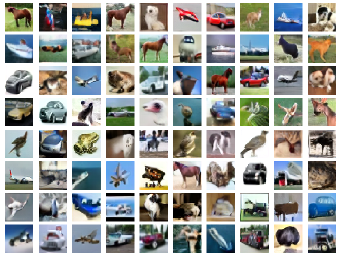
Figure 2: Example image samples generated by USD3^∗ as trained on VQCIFAR10. Most images are easy to recognize as being from one of the 10 classes in CIFAR10.

7.17.6 MCMC for Discrete-time and Continuous-time Discrete Diffusion

To demonstrate the effectiveness of MCMC corrector steps, we take the top performing methods in discrete and continuous time diffusion models (for discrete time, USD3^∗, and for continuous time USD3-CE) and show improved quality metrics over generated images after MCMC corrector is applied. Due to extensive time required for MCMC corrector step, we could only conduct evaluation over $5,000$ images, and thus the results are not comparable to the main VQCIFAR10 result in Table 2. We set the number of generation steps to be $100$ and use MCMC corrector on the last $10$, $20$ generation timesteps, respectively.

From the results shown in Table 8 and Table 9, we can see that MCMC corrector can significantly improve the quality of the generated samples. Specifically, for discrete-time generation, IS is showing a significant improvement than the sampling process without the MCMC corrector. For continuous-time case, both IS and FID scores are improving from the baseline (without MCMC).

Table 8: Image gen. quality w.r.t. Inception Score (IS) and the Frechet Inception Dist. (FID) over 5,000 samples unconditionally generated by USD3^∗ in discrete-time case. MCMC corrector is conducted for the last 10,20 timesteps over 100 sampling steps.

MCMC Configuration	IS (↑)	FID (↓)
Without MCMC	9.01	19.79
$\Delta n=0.001,N=2$, Start Steps:10	9.28	18.46
$\Delta n=0.001,N=2$, Start Steps:20	9.59	18.36
$\Delta n=0.005,N=2$, Start Steps:10	9.43	18.26
$\Delta n=0.005,N=2$, Start Steps:20	9.43	20.37
$\Delta n=0.001,N=5$, Start Steps:10	9.29	18.02
$\Delta n=0.001,N=5$, Start Steps:20	9.47	18.56
$\Delta n=0.002,N=5$, Start Steps:10	9.35	18.18
$\Delta n=0.002,N=5$, Start Steps:20	9.48	20.37

Table 9: Image gen. quality w.r.t. Inception Score (IS) and the Frechet Inception Dist. (FID) over 5,000 samples generated by USD3-CE in continuous-time case. MCMC corrector is conducted for the last 10,20 timesteps over 100 sampling steps.

MCMC Configuration	IS (↑)	FID (↓)
Without MCMC	8.98	19.19
$\Delta n=0.001,N=2$, Start Steps:10	9.12	17.62
$\Delta n=0.001,N=2$, Start Steps:20	9.23	17.35
$\Delta n=0.005,N=2$, Start Steps:10	9.01	17.71
$\Delta n=0.005,N=2$, Start Steps:20	9.23	17.58
$\Delta n=0.001,N=5$, Start Steps:10	9.03	17.26
$\Delta n=0.001,N=5$, Start Steps:20	9.00	17.42
$\Delta n=0.002,N=5$, Start Steps:10	9.16	17.98
$\Delta n=0.002,N=5$, Start Steps:20	8.97	17.83

References

- Anderson (2012) Anderson, W. J. Continuous-time Markov chains: An applications-oriented approach. Springer Science & Business Media, 2012.
- Austin et al. (2021) Austin, J., Johnson, D. D., Ho, J., Tarlow, D., and van den Berg, R. Structured denoising diffusion models in discrete state-spaces. Advances in Neural Information Processing Systems, 34:17981–17993, 2021.
- Brown et al. (2020) Brown, T., Mann, B., Ryder, N., Subbiah, M., Kaplan, J. D., Dhariwal, P., Neelakantan, A., Shyam, P., Sastry, G., Askell, A., et al. Language models are few-shot learners. Advances in neural information processing systems, 33:1877–1901, 2020.
- Campbell et al. (2022) Campbell, A., Benton, J., De Bortoli, V., Rainforth, T., Deligiannidis, G., and Doucet, A. A continuous time framework for discrete denoising models. Advances in Neural Information Processing Systems, 35:28266–28279, 2022.
- Chang et al. (2022) Chang, H., Zhang, H., Jiang, L., Liu, C., and Freeman, W. T. Maskgit: Masked generative image transformer, 2022.
- Chen (2023) Chen, T. On the importance of noise scheduling for diffusion models. arXiv preprint arXiv:2301.10972, 2023.
- Demirkaya et al. (2020) Demirkaya, A., Chen, J., and Oymak, S. Exploring the role of loss functions in multiclass classification. In 2020 54th annual conference on information sciences and systems (ciss), pp. 1–5. IEEE, 2020.
- Deng et al. (2009) Deng, J., Dong, W., Socher, R., Li, L.-J., Li, K., and Fei-Fei, L. Imagenet: A large-scale hierarchical image database. In 2009 IEEE Conference on Computer Vision and Pattern Recognition, pp. 248–255, 2009. doi: 10.1109/CVPR.2009.5206848.
- Dhariwal & Nichol (2021) Dhariwal, P. and Nichol, A. Diffusion models beat gans on image synthesis. Advances in neural information processing systems, 34:8780–8794, 2021.
- Dong et al. (2017) Dong, H.-W., Hsiao, W.-Y., Yang, L.-C., and Yang, Y.-H. Musegan: Multi-track sequential generative adversarial networks for symbolic music generation and accompaniment, 2017.
- Esser et al. (2020) Esser, P., Rombach, R., and Ommer, B. Taming transformers for high-resolution image synthesis, 2020.
- Gillespie (1977) Gillespie, D. T. Exact stochastic simulation of coupled chemical reactions. The journal of physical chemistry, 81(25):2340–2361, 1977.
- Gillespie (2001) Gillespie, D. T. Approximate accelerated stochastic simulation of chemically reacting systems. The Journal of chemical physics, 115(4):1716–1733, 2001.
- Ho et al. (2020a) Ho, J., Jain, A., and Abbeel, P. Denoising diffusion probabilistic models. Advances in Neural Information Processing Systems, 33:6840–6851, 2020a.
- Ho et al. (2020b) Ho, J., Jain, A., and Abbeel, P. Denoising diffusion probabilistic models. Advances in neural information processing systems, 33:6840–6851, 2020b.
- Ho et al. (2022) Ho, J., Chan, W., Saharia, C., Whang, J., Gao, R., Gritsenko, A., Kingma, D. P., Poole, B., Norouzi, M., Fleet, D. J., et al. Imagen video: High definition video generation with diffusion models. arXiv preprint arXiv:2210.02303, 2022.
- Hoogeboom et al. (2021) Hoogeboom, E., Nielsen, D., Jaini, P., Forré, P., and Welling, M. Argmax flows and multinomial diffusion: Learning categorical distributions. Advances in Neural Information Processing Systems, 34:12454–12465, 2021.
- Hyvärinen (2007) Hyvärinen, A. Some extensions of score matching. Computational statistics & data analysis, 51(5):2499–2512, 2007.
- Kang & Cho (2018) Kang, S. and Cho, K. Conditional molecular design with deep generative models. Journal of chemical information and modeling, 59(1):43–52, 2018.
- Karras et al. (2022) Karras, T., Aittala, M., Aila, T., and Laine, S. Elucidating the design space of diffusion-based generative models. Advances in Neural Information Processing Systems, 35:26565–26577, 2022.
- Kolmogoroff (1931) Kolmogoroff, A. Über die analytischen methoden in der wahrscheinlichkeitsrechnung. Mathematische Annalen, 104:415–458, 1931.
- Li et al. (2022) Li, X., Thickstun, J., Gulrajani, I., Liang, P. S., and Hashimoto, T. B. Diffusion-lm improves controllable text generation. Advances in Neural Information Processing Systems, 35:4328–4343, 2022.
- Li et al. (2021) Li, Y., Pei, J., and Lai, L. Structure-based de novo drug design using 3d deep generative models. Chemical science, 12(41):13664–13675, 2021.
- Lyu (2009) Lyu, S. Interpretation and generalization of score matching. In Proceedings of the Twenty-Fifth Conference on Uncertainty in Artificial Intelligence, pp. 359–366, 2009.
- OpenAI (2023) OpenAI. Gpt-4 technical report. ArXiv, abs/2303.08774, 2023. URL https://arxiv.org/abs/2303.08774.
- Raffel (2016) Raffel, C. Learning-Based Methods for Comparing Sequences, with Applications to Audio-to-MIDI Alignment and Matching. PhD thesis, Columbia University, 2016.
- Ramesh et al. (2022) Ramesh, A., Dhariwal, P., Nichol, A., Chu, C., and Chen, M. Hierarchical text-conditional image generation with clip latents. arXiv preprint arXiv:2204.06125, 1(2):3, 2022.
- Rindos et al. (1995) Rindos, A., Woolet, S., Viniotis, I., and Trivedi, K. Exact methods for the transient analysis of nonhomogeneous continuous time markov chains. In Computations with Markov Chains: Proceedings of the 2nd International Workshop on the Numerical Solution of Markov Chains, pp. 121–133. Springer, 1995.
- Song et al. (2021a) Song, J., Meng, C., and Ermon, S. Denoising diffusion implicit models. In International Conference on Learning Representations, 2021a. URL https://openreview.net/forum?id=St1giarCHLP.
- Song et al. (2021b) Song, Y., Sohl-Dickstein, J., Kingma, D. P., Kumar, A., Ermon, S., and Poole, B. Score-based generative modeling through stochastic differential equations. In International Conference on Learning Representations, 2021b. URL https://openreview.net/forum?id=PxTIG12RRHS.
- Sun et al. (2023) Sun, H., Yu, L., Dai, B., Schuurmans, D., and Dai, H. Score-based continuous-time discrete diffusion models. In The Eleventh International Conference on Learning Representations, 2023. URL https://openreview.net/forum?id=BYWWwSY2G5s.
- Tewari & Bartlett (2007) Tewari, A. and Bartlett, P. L. On the consistency of multiclass classification methods. Journal of Machine Learning Research, 8(5), 2007.
- van den Oord et al. (2018) van den Oord, A., Vinyals, O., and Kavukcuoglu, K. Neural discrete representation learning, 2018.
- Zhang et al. (2023) Zhang, C., Zhang, C., Zhang, M., and Kweon, I. S. Text-to-image diffusion model in generative ai: A survey. arXiv preprint arXiv:2303.07909, 2023.
- Zheng et al. (2023) Zheng, L., Yuan, J., Yu, L., and Kong, L. A reparameterized discrete diffusion model for text generation. arXiv preprint arXiv:2302.05737, 2023.