Abstract

The local learning coefficient (LLC) is a principled way of quantifying model complexity, originally derived in the context of Bayesian statistics using singular learning theory (SLT). Several methods are known for numerically estimating the local learning coefficient, but so far these methods have not been extended to the scale of modern deep learning architectures or data sets. Using a method developed in Lau et al. (2023) we empirically show how the LLC may be measured accurately and self-consistently for deep linear networks (DLNs) up to 100M parameters. We also show that the estimated LLC has the rescaling invariance that holds for the theoretical quantity.

1 Introduction

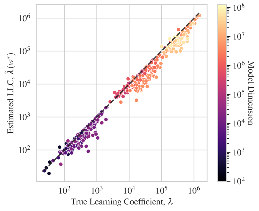
Figure 1: Estimated local learning coefficient against true learning coefficient; model dimension shown in color. The estimated LLC accurately measures the learning coefficient $\lambda$ up to 100 million parameters in deep linear networks, as compared to known theoretical values (dashed line). See Figure 10 for linear-scale plots.

It is now abundantly clear that deep learning works. The question now is whether we can understand why it works and what kind of internal structures develop in these networks in order to represent information about the world and compute on that information. This is a very difficult problem, on which it is hard to make progress without fundamental advances in our ability to make quantitative measurements of these internal structures.

The parameter count, which in classical statistical learning theory is one appropriate measure of the amount of information captured in a fitted model, is well-known to be inappropriate in deep learning. This is clear from technical results on generalization Zhang et al. (2017), pruning Blalock et al. (2020) and distillation Hinton et al. (2015) but it also common sense: the amount of information captured in a trained network is in some sense decoupled from the number of parameters.

However, it is far from clear a priori what the replacement for counting parameters should be. With this in mind, it is notable that within Bayesian learning theory, there already exists a way to formalize this notion: the learning coefficient of SLT Watanabe (2009). The learning coefficient was originally introduced by Watanabe (2001) to predict generalization in singular models like neural networks, where it completely replaces the parameter count term in the formula for generalization error (see Section 2 and Appendix A.2). In this setting, it has seen significant practical application (e.g. Endo et al., 2020; Fontanesi et al., 2019; Hooten & Hobbs, 2015; Sharma, 2017; Kafashan et al., 2021; Semenova et al., 2020).

Beyond its role in generalization, the learning coefficient can be viewed as a natural invariant of the local geometry of the population loss. It also has an information-theoretic interpretation that makes sense without any of the machinery of Bayesian statistics, as we show in Section 2. This brings us to the goal of the present work: to import this principled measure of model complexity from Bayesian statistics into machine learning more generally, and apply it at scale.

Unfortunately for this plan, the learning coefficient has historically been difficult to measure. It can be calculated theoretically in some rare cases Yamazaki & Watanabe (2003); Aoyagi et al. (2005); Aoyagi (2024), but has not yet been calculated for any deep (nonlinear) neural networks. Watanabe (2013) showed that the learning coefficient may be estimated numerically using Markov Chain Monte Carlo (MCMC), but traditional MCMC algorithms are inefficient for the large dataset sizes found in modern machine learning.

Lau et al. (2023) showed how Watanabe’s definitions may be modified to define a local learning coefficient (LLC) and how this can be estimated at larger scale using stochastic-gradient MCMC. However, based on the evidence shown in their work, it was not clear that the LLC estimator considered was in fact accurately estimating the learning coefficient, particularly for large neural networks.

Our contributions. In this paper, we conduct a comprehensive evaluation of the Lau et al. (2023) stochastic-gradient LLC estimator:

• Accuracy. We compare the stochastic-gradient method against a prior “full-gradient” method in small ReLU networks and find it produces near identical outputs; and against theoretical predictions in deep linear networks (DLN), and find that it successfully recovers the true learning coefficient.

• Scalability. Our ReLU network experiments confirm that the stochastic-gradient method becomes significantly faster than full-gradient methods as dataset size increases. Our DLN experiments go up to 100M parameters, where full-gradient methods are too slow to feasibly use.

• Self-consistency. Dinh et al. (2017) showed that some loss geometry measures are sensitive to rescaling symmetries in ReLU networks. We show empirically that Dinh et al. (2017)’s concerns do not apply to learning coefficient estimation.

In doing so, we prove that the LLC can be accurately estimated at far greater scale than ever before, opening the door for the LLC to be applied to modern machine learning.

2 The (local) learning coefficient

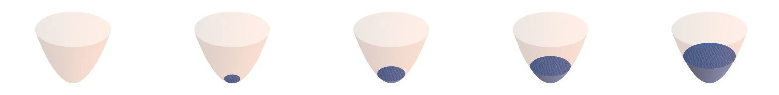
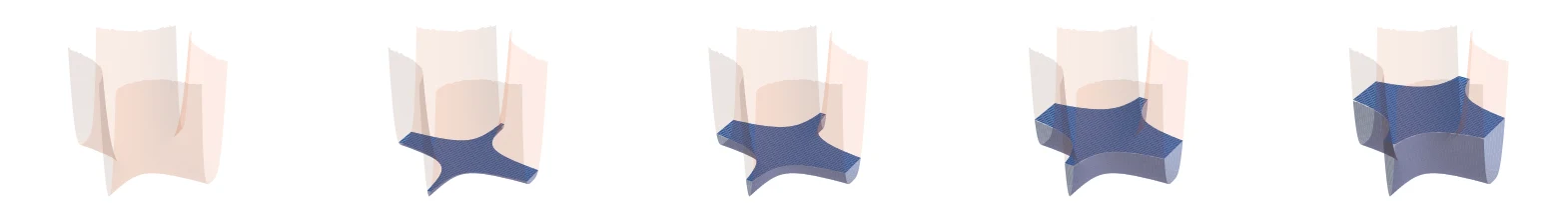
Figure 2: The learning coefficient $\lambda$ measures volume scaling. Top: the area (or “2D-volume”) under the loss $L(w_{1},w_{2})={w_{1}}^{2}+{w_{2}}^{2}$ scales as $V(\epsilon)\propto\epsilon$, so $\lambda=1$. Bottom: the area under the loss $L(w_{1},w_{2})={w_{1}}^{2}{w_{2}}^{4}$ scales as $V(\epsilon)\propto\epsilon^{1/4}$, so $\lambda=\frac{1}{4}$. Lower $\lambda$ means more volume: as we approach the minimum ($\epsilon\rightarrow 0$), there is much more volume available for the bottom loss function compared to the top for any given small tolerance $\epsilon$. Reproduced with permission from Hoogland & Van Wingerden (2023).

We define the learning coefficient together with its localized version and review the intuition behind these quantities. For the full details we refer the reader to Appendix A and prior sources (Watanabe, 2009; Lau et al., 2023) — here we focus on providing some practical insight into what the LLC is measuring. The learning coefficient can be defined in many equivalent ways; here we define it as an invariant based on loss landscape basin volume to emphasise its geometric intuition separate from its statistical implications.

2.1 Complexity via counting low loss parameters

In machine learning, we aim to minimize a loss function $L_{n}(w)$ to find the best parameter fitting a given target distribution (or target function). However, we only have access to the target distribution via a finite set of $n$ training samples $D_{n}=\{X_{1},\dots,X_{n}\}$, so we may be mistaken about which parameter is actually best — we will likely select a parameter that is slightly worse than the best parameter.

This naturally leads to the question: “how many parameters are almost as good as the best parameter?” This is the perspective taken by Hochreiter & Schmidhuber (1997), following the literature on the minimum description length (Grünwald & Roos, 2019), in attempting to quantify the complexity of a trained neural network. (We discuss the sense in which we use the term “complexity” in Appendix C.)

We can formalize this by defining $V(\epsilon)$ to be the volume of the set of parameters whose loss is within $\epsilon$ of the minimum Dinh et al. (2017). The idea is to measure the complexity of a network by measuring the number of bits that it takes to specify the low loss subset of the parameter space $W$. That is, if the subset of parameters in $W$ with loss less than $\epsilon$ requires many bits to specify — i.e. $-\log(V(\epsilon)/\operatorname{Vol}(W))$ is large — then it is complex. However, there are two subtle problems with this notion, the resolution of which will lead us to the LLC.

The first is a conceptual problem: it is not clear what it means for a parameter to be “low loss” in an absolute sense, since the loss function $L_{n}(w)$ depends on the training samples taken, rather than the underlying data generating process — it is a random variable depending on $D_{n}$. We can average this out by using the population loss $L(w)=\mathbb{E}_{D_{n}}[L_{n}(w)]$ instead. This is an important theoretical distinction.

The second, more difficult problem is that, in order for $V(\epsilon)$ to not depend on an arbitrary choice of $\epsilon$, one must know the functional dependence of $V(\epsilon)$ on $\epsilon$ — this turns out to be very difficult in general. Classically, it is assumed that $L$ is locally quadratic, and so the volume satisfies a law of the form

$$V(\epsilon)\approx c\epsilon^{d/2}$$

where $c$ is a constant that depends on the curvature of the basin at its minimum, and $d$ is the dimension of $W$. In this case the meaningful quantity is the constant $c$, which can be easily extracted by taking $-\log(V(\epsilon)/\epsilon^{d/2})=\log c$. See top row of Figure 2 for a 2D example.

However when $L$ is the population loss of a neural network, the volume dependence on $\epsilon$ is highly nontrivial, and has an exponent that is not only different to $d/2$, but which depends on the training data!

2.2 The definition

In fact, the correct volume scaling exponent in general is given by the learning coefficient.

Definition 2.1 (The learning coefficient, $\lambda$).

Let $L_{0}:=\min_{w\in W}L(w)$ denote the minimum population loss. For any $\epsilon>0$, define $V(\epsilon)$ as the Lebesgue volume of the set $\{w\in W\mid L(w)-L_{0}<\epsilon\}$. There exists a unique rational number $\lambda$ and a positive integer $m$ such that the following proportionality holds asymptotically as $\epsilon\to 0$:

$$V(\epsilon)\propto\epsilon^{\lambda}(-\log(\epsilon))^{m-1}$$ (1)

We call $\lambda$ the learning coefficient, and $m$ the multiplicity Watanabe (2009).

We define the local learning coefficient $\lambda(w^{*})$ around any local minimum $w^{*}$ in a similar manner, except we restrict to a sufficiently small neighbourhood $N(w^{*})\subset W$ of $w^{*}$ so that the volume of concern is instead that of the set $\{w\in N(w^{*})\mid L(w)-L(w^{*})<\epsilon\}$.

In the case where $m=1$, the formula simplifies, and the intuition behind $\lambda$ becomes clear:

$$V(\epsilon)\propto\epsilon^{\lambda}$$ (2)

Thus, the learning coefficient $\lambda$ is the (asymptotic) volume scaling exponent near a minimum in the loss landscape: increasing the error tolerance by a factor of $c$ increases the volume by a factor of $c^{\lambda}$. This makes $\lambda$ into a kind of fractional dimension; in the sense that, when $\lambda$ is an integer, Eq 2 implies that $V(\epsilon)$ scales similarly to a $\lambda$-dimensional hypercube with side length $\epsilon$.

This also suggests an intuitive information-theoretic interpretation. Informally,

$$-\log_{2}\frac{V(\epsilon)}{\mathrm{Vol}(W)}=-\lambda\log_{2}\epsilon+O(\log\log\epsilon)$$

represents the number of bits required to specify a parameter in the parameter space $W$ to within the subspace that has at most $\epsilon$ error. We observe that this asymptotic scaling exponent of $V(\epsilon)$ tells us the amount of additional information needed to halve an already small error of $\epsilon$:

$$-\log_{2}\frac{V\left(\frac{\epsilon}{2}\right)}{\mathrm{Vol}(W)}+\log_{2}\frac{V(\epsilon)}{\mathrm{Vol}(W)}$$

$$\approx-\lambda\log_{2}\frac{\epsilon}{2}+\lambda\log_{2}\epsilon$$

$$=\lambda$$

This perspective hints at a potential connection to generalization error: $\lambda$ determines the rate at which additional data rule out parameters that no longer fit the larger dataset. Indeed, in the Bayesian setting, Watanabe (2009) proved that $\lambda$ determines the rate at which the posterior mass concentrates around the global minima of the loss, which in turn implies an asymptotic formula for the Bayesian generalization error, $G(n)$

$$G(n)=L_{n}(w_{0})+\frac{\lambda}{n}+O\left(\frac{1}{n}\right)$$ (3)

as dataset size $n\to\infty$ and $w_{0}$ is any minimum of $L(w)$ . (Further details in Appendix A.2.)

In this way, methods for estimating the learning coefficient are automatically methods for estimating Bayesian generalization error, and have been used successfully to this effect in a variety of statistical and machine learning models (e.g. Endo et al., 2020; Fontanesi et al., 2019; Hooten & Hobbs, 2015; Sharma, 2017; Kafashan et al., 2021; Semenova et al., 2020).

It is also worth noting that $\lambda$ has a natural interpretation from a statistical mechanics perspective. If one interprets the loss function $L(w)$ as a potential energy function, then $\lambda$ is the low-temperature specific heat of the system LaMont & Wiggins (2019). In physics, studying the low-temperature specific heat of materials was foundational to the field of solid-state physics Ashcroft & Mermin (2022).

3 Practical estimation of the learning coefficient

3.1 MCMC-based learning coefficient estimation

In Watanabe (2013), it was shown that the learning coefficient may be estimated via MCMC.

Specifically, let $L_{n}(w)$ be the loss function with dataset size $n$ as before, then we have an estimator for the learning coefficient

$$\hat{\lambda}=\frac{1}{\beta}\left(\mathbb{E}_{w}^{\beta}[nL_{n}(w)]-nL_{n}(w^{*})\right)$$ (4)

where $\mathbb{E}_{w}^{\beta}[-]$ denote expectation over the tempered posterior distribution given by $p(w\,|\,D_{n})\propto e^{-\beta nL_{n}(w)}$ at inverse temperature $\beta>0$. A theorem by Watanabe (2013) can be shown to imply that this is an asymptotically unbiased estimator of the learning coefficient if the inverse temperature is set to

$$\beta\approx\frac{1}{\log n}$$ (5)

This formula is the basis for all empirical learning coefficient estimation in this paper.

3.2 Stochastic-gradient LLC estimator, $\hat{\lambda}(w^{*})$

Unfortunately, this has several practical difficulties in larger models, which subsequent work by Lau et al. (2023) has addressed.

First, this method has historically been used to measure the global, rather than local learning coefficient — a far more difficult prospect for large models, as this implicitly requires the posterior sampler to find and sample from (the neighbourhood of) global minima in high dimension. Lau et al. (2023) explicitly focuses on the local quantity, adding a quadratic confinement term to the loss function to keep MCMC exploration in the neighborhood of the target point. This amounts to defining an LLC estimator, $\hat{\lambda}(w^{*})$, at an local minimum $w^{*}$ of the loss:

$$\hat{\lambda}(w^{*})=\frac{1}{\beta}\left(\mathbb{E}_{w\mid w^{*}}^{\beta}[nL_{n}(w)]-nL_{n}(w^{*})\right)$$ (6)

where $\mathbb{E}_{w\mid w^{*}}^{\beta}[-]$ is a now an expectation over the localized tempered posterior,

$$p(w\,|\,D_{n},w^{*})\propto e^{-\beta nL_{n}(w)-\gamma\|w-w^{*}\|^{2}}$$

where $\gamma>0$ is a hyperparameter tuning the confinement strength.

A second problem is that the dataset sizes in modern ML are typically too large to efficiently perform full-batch gradient calculations, which are required to perform exact MCMC. If one substitutes full-batch gradients for minibatch gradients, this results in stochastic gradient MCMC, a prototypical example of which is stochastic gradient Langevin dynamics (SGLD) introduced by Welling & Teh (2011). This improves efficiency for large dataset sizes, with the drawback that formal guarantees of unbiased posterior sampling are lost.

Lau et al. (2023) applies SGLD to LLC estimation, resulting in a quantity which we shall call stochastic-gradient LLC estimator. This is the technique explored in this paper. The formula for $\hat{\lambda}(w^{*})$ is the one given in Equation 6 — it is only the sampling method used to evaluate the expectation value that changes. Specifically, the update function that generate a sampling chain is given by:

$$\Delta w_{t+1}=A\frac{\epsilon}{2}\left(\frac{\beta n}{m}\sum_{i=1}^{m}\nabla nL_{n}(w_{t})+\gamma(w^{*}-w_{t})\right)$$

$$+N(0,A\epsilon)$$

where $\epsilon$ is the step size, $\gamma$ the confinement strength, $m$ is the minibatch size, $n$ is the dataset size, $\beta$ is the same inverse temperature parameter from Section 3.1, and $w^{*}$ is the location of the local minima in question. The formula given here differs from that given in Lau et al. (2023) only in the addition of $A$, the (optional) preconditioning matrix, which we assume to be the identity unless stated otherwise.

4 Experiments and results

Lau et al. (2023) supported their stochastic-gradient LLC estimation method by demonstrating that it can recover the true learning coefficient but only for toy 2-dimensional models, has low variance over independent sampling runs for moderately large models ($\approx 2M$ parameters). However, that is not sufficient to know whether or not the estimator is accurate for neural networks at practical scale. In this paper, we experimentally provide evidence that stochastic-gradient LLC estimator is indeed a scalable, accurate, and self-consistent measure of the learning coefficient. We conclude this from the following evidence:

• Due to a recent result by Aoyagi (2024), we can theoretically predict the value of the learning coefficient for deep linear networks (DLNs), making them the closest models to modern machine learning for which such theoretical values are available. We show that stochastic-gradient LLC estimator can accurately recover the theoretically predicted learning coefficient for DLNs up to at least 100M parameters. (Section 4.2)

• We directly compare stochastic-gradient LLC estimator with full-gradient MCMC method in ReLU networks small enough to feasibly compare the two. We find that the two methods agree almost exactly, but stochastic-gradient LLC estimator is much more efficient. (Section 4.1)

• With proper preconditioning, stochastic-gradient LLC estimator is invariant to parameter-space symmetries, like rescaling symmetries in ReLU networks. (Section 4.3)

4.1 Stochastic-gradient LLC estimator is just as accurate, but faster

It is worth repeating that, as discussed in Section 3.2, the modifications introduced by Lau et al. (2023) in creating stochastic-gradient LLC estimator lead to a loss of theoretical guarantee that its estimates will be unbiased. This means that to claim stochastic-gradient LLC estimator is in fact a practical LLC estimator, we must at least verify empirically that it is no worse than the prior method.

Specifically, we compare learning coefficient estimation with SGLD Lau et al. (2023) with learning coefficient estimation via the Metropolis-adjusted Langevin Algorithm (MALA), a standard gradient-based MCMC algorithm Roberts & Rosenthal (1998).

Here we test with a two-hidden-layer ReLU network with ten inputs, ten outputs, and twenty neurons per hidden layer. Denote the inputs by $x$, the parameters by $w$, and the output of this network $f(x,w)$. The data are generated to create a “realizable” data generating process, with “true parameter” $w^{*}$: inputs $X$ are generated from a uniform distribution, and labels $Y$ are generated based on the true network, so that $Y_{i}=f(X_{i},w^{*})$.

We sweep dataset size from 100 to 100000, and compare SGLD and MALA. For all dataset sizes, SGLD batch size was set to 32 and SGLD $\gamma=1.0$, and MALA and SGLD shared the same true parameter $w^{*}$ (set at random according to a normal distribution). Both MALA and SGLD used a step size of 1e-5, the learning coefficient formula given in Section 3.1, and the asymptotically optimal temperature given by Eq 5. Experiments were run on CPU.

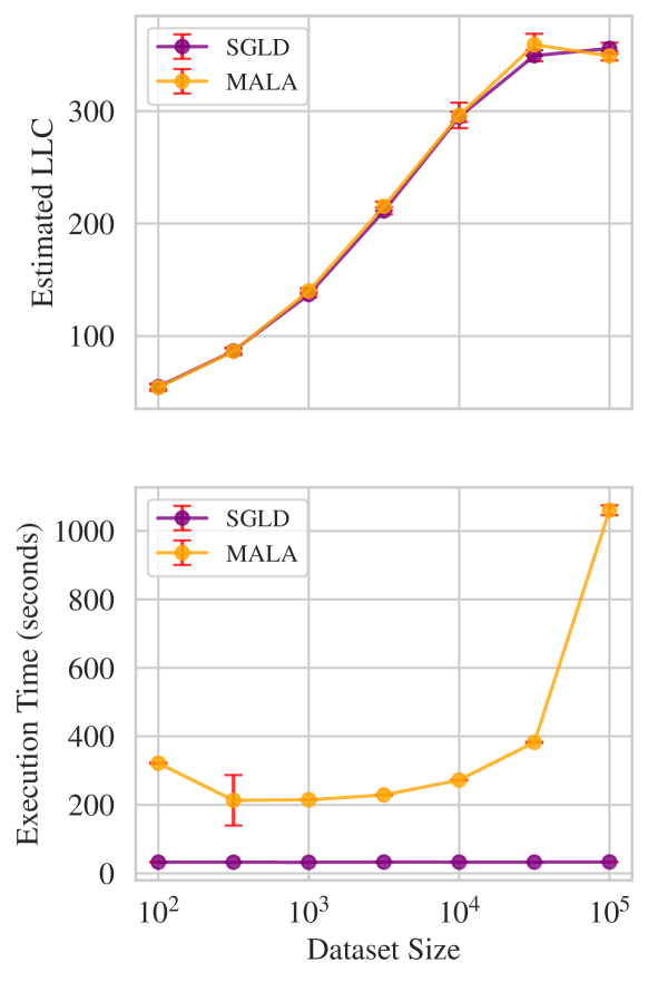
Figure 3: We compare learning coefficient estimation using SGLD Lau et al. (2023) with learning coefficient estimation using MALA. They make similar estimates (top) but the SGLD-based method is significantly faster (bottom), especially for large dataset sizes.

The results are summarized in Figure 3. We find that across all dataset sizes: 1. the SGLD and MALA estimates of the learning coefficient agree (Figure 3, top) 2. but the SGLD-based estimate has far lower computational cost, especially as the dataset size grows (Figure 3, bottom).

4.2 Stochastic-gradient LLC estimator is accurate at large scale

The advantage of stochastic-gradient LLC estimator over the prior full-gradient $\hat{\lambda}(w^{*})$ is its scalability. However, in order for this advantage to actually materialize, it must be scalably accurate, as we verify here for DLNs —- the most realistic setting where we have theoretical ground truth values for the learning coefficient.

A DLN is a feedforward neural network without nonlinear activation. Specifically, a biasless DLN with $M$ hidden layers, layer sizes $H_{1},H_{2},\dots,H_{M}$ and input dimension $H_{0}$ is given by:

$$y=f(x,w)=W_{M}\ldots W_{2}W_{1}x$$ (7)

where $x\in\mathbb{R}^{H_{0}}$ is the input vector and the model parameter $w$ consist of the weight matrices $W_{j}$ of shape $H_{j}\times H_{j-1}$ for $j=1,\dots,M$.

The input-output behavior of a DLN is obviously trivial; it is equivalent to a single-layer linear network obtained by multiplying together the weight matrices. However, the geometry of such a model is highly non-trivial — in particular, the optimization dynamics and inductive biases of such networks have seen significant research interest Saxe et al. (2013); Ji & Telgarsky (2018); Arora et al. (2018).

To establish the accuracy of stochastic-gradient LLC estimator for DLN, we shall compare it to the theoretical learning coefficient recently derived via algebro-geometric calculation by Aoyagi (2024). See Appendix B for details and further discussions.

Here we shall pause and emphasize that this result gives us the (global) learning coefficient, which is conceptually distinct from the LLC. They are related: the learning coefficient is the minimum of the LLCs (of the global minima of the population loss). In our experiments, we will be measuring the LLC at a randomly chosen global minimum of the population loss. While we expect those values to be close, we do not know that for certain and it is of independent interest that the estimated LLC can tell us about the learning coefficient.

We compare the estimated $\hat{\lambda}(w^{*})$ against theoretical $\lambda$ (with $w^{*}$ being a randomly generated true parameter), by randomly generating many DLNs with different architectures and model sizes that span several orders of magnitude (OOM). Each DLN is constructed randomly, as follows. Draw an integer $M\sim U(M_{low},\dots,M_{high})$ as the number of hidden layers, where $U(a,\dots,b)$ denotes the discrete uniform distribution on the finite set $\{a,a+1,\dots,b\}$. Then, draw layer size $H_{j}\sim U(H_{low},\dots,H_{high})$ for each $j=0,\dots,M$ where $H_{0}$ denotes the input dimension. The weight matrix $W_{j}$ for layer $j$ is then a $H_{j}\times H_{j-1}$ matrix with each matrix element independently sampled from $N(0,1)$ (random initialization). To obtain a more realistic true parameter, with probability $0.5$, each matrix $W_{j}$ is modified to have a random rank of $r\sim U(0,\dots,\min(H_{j-1},H_{j}))$. For each DLN generated, a corresponding synthetic training dataset of size $n$ is generated to be used in SGLD sampling.

The configuration values $M_{low},M_{hight},H_{low},H_{high}$ are chosen differently for separate set of experiments with model size targeting DLN size of different order of magnitude. SGLD hyperparameters $\epsilon$, $\gamma$, and number of steps are chosen to suit each set of experiments according to our recommendations outlined in Appendix D. These values are detailed in Appendix E.1.

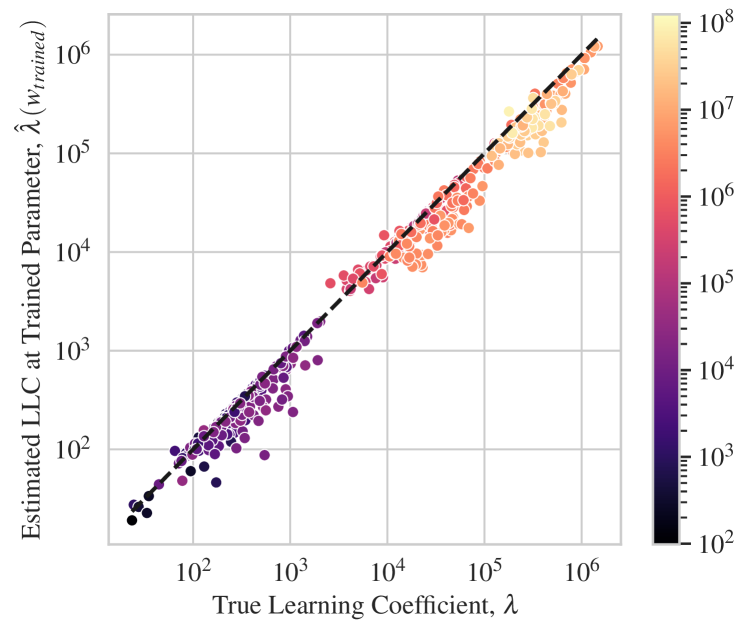
Figure 4: $\hat{\lambda}(w^{*})$ against theoretical learning coefficient for DLNs, with $w^{*}$ being the final parameter of an SGD training run.

The results are summarized in Figure 1. stochastic-gradient LLC estimator is able to accurately estimate the learning coefficient up to 100M parameters for DLNs. We further show that accuracy is maintained even if (as is typical in practice) one does not initialize at the global minimum, but is instead forced to use SGD to first find a minimum. The results can be seen in Figure 4 and experimental configurations are detailed in Appendix E.1.

We run one final set of DLN experiments that track a modified (see Appendix E.2) version of $\hat{\lambda}(w^{*})$ over the course of SGD training. We notice that the estimated LLC can measure changes in a model’s internal structure. This is conceptually similar to the experiments of Chen et al. (2023) and Hoogland et al. (2024) — in our case, the internal structure in question is the model’s rank.

Our experiments mirror the setup in Jacot et al. (2021), where they reported theoretical and experiment evidence for “saddle-to-saddle” training dynamics: the DLN gradient descent trajectory, when initialised with Gaussian $N(0,\sigma^{2}=H^{-\delta})$ for $\delta>1$, visits neighbourhoods of a sequence of saddle points of the loss landscape that correspond to the DLN implementing linear maps of increasing rank. Results, plotted in Figure 5, confirm that $\hat{\lambda}(w^{*})$ can quickly detect when the trajectory moves to a different saddle. In the case of DLNs, $\hat{\lambda}(w^{*})$ is not needed to detect these changes — they are directly visible in the training loss and other metrics like the nuclear norm. However, in more general situations, $\hat{\lambda}(w^{*})$ detects changes that other measures do not Chen et al. (2023); Hoogland et al. (2024).

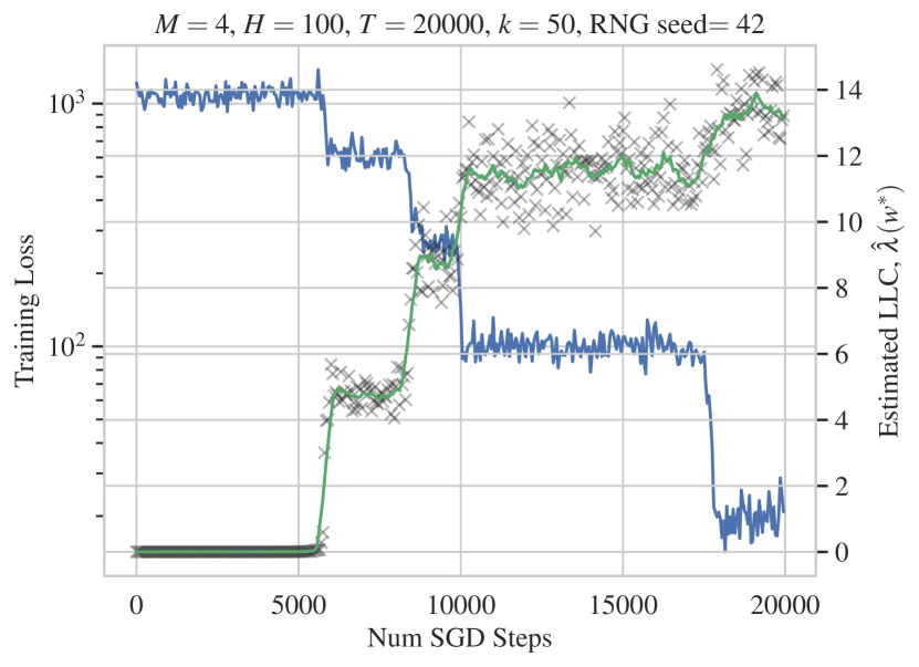
Figure 5: $\hat{\lambda}(w^{*})$ can detects known local geometry changes along the “saddle-to-saddle” training trajectory for DLNs. Decreases in SGD training loss (blue) are matched by increases in estimated LLC (grey crosses, green line).

4.3 Stochastic-gradient LLC estimator is rescaling-invariant

Here we empirically verify that stochastic-gradient learning coefficient estimators inherit an important self-consistency property of the learning coefficient.

In particular, the LLC is invariant to global parameter-space symmetries. The most well-known example of this is “rescaling symmetry” in feedforward ReLU networks, which we describe shortly. Invariance to this symmetry is not trivial or automatic, and other geometric measures like Hessian-based basin broadness have been undermined by their failure to stay invariant to these symmetries Dinh et al. (2017).

For simplicity, suppose we have a two-layer ReLU network, with weights $W_{1},W_{2}$ and biases $b_{1},b_{2}$. Then rescaling symmetry is captured by the following fact, for some arbitrary scalar $\alpha$:

$$W_{2}\text{ReLU}(W_{1}x+b_{1})+b_{2}=\alpha W_{2}\text{ReLU}\left(\tfrac{1}{\alpha}W_{1}x+\tfrac{1}{\alpha}b_{1}\right)+b_{2}$$

That is, we may choose new parameters $W_{1}^{\prime}=\frac{1}{\alpha}W_{1},b_{1}^{\prime}=\frac{1}{\alpha}b_{1},W_{2}^{\prime}=\alpha W_{2},b_{2}^{\prime}=b_{2}$ without affecting the input-output behavior of the network in any way. This symmetry generalizes to any two adjacent layers in ReLU networks of arbitrary depth.

Given that these symmetries do not affect the function implemented by the network, and are present globally throughout all of parameter space, it seems like these degrees of freedom are “superfluous”, and should ideally not affect our tools. Importantly, this is the case for the learning coefficient.

We verify empirically that this property also appears to hold for stochastic-gradient learning coefficient estimators, when proper preconditioning is used.

Specifically, we take a small feedforward ReLU network, and rescale two adjacent layers in the network by $\alpha$ in the fashion described above. We vary the value of $\alpha$ across eight orders of magnitude and measure the estimated learning coefficient. Crucially, we must use preconditioning here so as to avoid prohibitively small step size requirements. In this case, the preconditioning matrix $A$ is set manually, to be a diagonal matrix with entries $\alpha^{2}$ for parameters corresponding to $W_{1}$ and $b_{1}$, entries $\frac{1}{\alpha^{2}}$ for $W_{2}$, and entries $1$ otherwise.

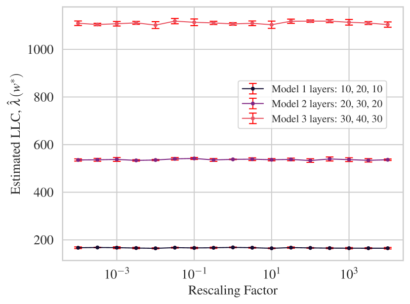
Figure 6: Stochastic-gradient learning coefficient estimation is invariant to rescaling symmetries in ReLU networks. As the rescaling parameter $\alpha$ is varied over eight orders of magnitude, the estimated value of the learning coefficient remains invariant (up to statistical error). The small error bar across multiple SGLD runs illustrates the stability of the estimation method. Model layer sizes, including input dimension is shown in the legend.

The results can be found in Figure 6. We conclude that stochastic-gradient learning coefficient estimation appears invariant to ReLU network rescaling symmetries.

5 Related Work

We review both the singular learning theory literature directly involving the learning coefficient, as well as research from other areas of machine learning that may be relevant.

Singular learning theory. The learning coefficient was first introduced by Watanabe (2001) in the context of Bayesian statistics, where he proved that it determines the leading order term of the expected Bayesian generalization error, as we review in Appendix A.2. Later work used algebro-geometric tools to bound or exactly calculate the learning coefficient for a wide range of machine learning models, including Boltzmann machines Yamazaki & Watanabe (2005a), single-hidden-layer neural networks Aoyagi et al. (2005), DLNs Aoyagi (2024), Gaussian mixture models Yamazaki & Watanabe (2003), and hidden Markov models Yamazaki & Watanabe (2005b).

The difficulty of these calculations lead Watanabe (2013) to introduce an empirical estimator of the learning coefficient (and correspondingly, of the Bayesian generalization error and model evidence), which we review in Section 3.1. In its role as an estimate of model evidence, it is called the WBIC, and has been used practically in a wide range of applied settings (e.g. Endo et al., 2020; Fontanesi et al., 2019; Hooten & Hobbs, 2015; Sharma, 2017; Kafashan et al., 2021; Semenova et al., 2020). Several other papers have explored improvements or alternatives to this estimator Iriguchi & Watanabe (2007); Imai (2019a; b), though none address the issue of large dataset sizes.

In order to improve the scalability of this method to large dataset sizes, Lau et al. (2023) introduced stochastic-gradient learning coefficient estimation — the main subject of this paper, and which we review in Section 3.2. Recently, the Lau et al. (2023) method has been used to empirically measure “phase transitions” in deep learning Chen et al. (2023), and the development of in-context learning in transformers Hoogland et al. (2024).

However, Lau et al. (2023) pitched their method merely as a model complexity measure inspired by the learning coefficient, but did not claim their method accurately measured the learning coefficient. As our primary contribution, we empirically confirm the latter, stronger claim, allowing the Lau et al. (2023) method to legitimately claim to be a learning coefficient estimator, at least for deep linear networks.

Basin broadness. The learning coefficient can be seen as a Bayesian version of basin broadness measures, which typically attempt to empirically connect notions of geometric “broadness” or “flatness” with (non-Bayesian) generalization error Hochreiter & Schmidhuber (1997); Jiang et al. (2019). However, the evidence supporting the learning coefficient (in the Bayesian setting) is significantly stronger: the learning coefficient provably determines the Bayesian generalization error to leading order (see Appendix A.2). We expect the utility of the learning coefficient as a geometric measure to apply beyond the Bayesian setting, but whether the connection with generalization will continue to hold is unknown.

Neural network identifiability. A core observation leading to singular learning theory is that the map $w\mapsto p(x|w)$ from parameters $w$ to statistical models $p(x|w)$ may not be one-to-one (in which case, the model is singular). This observation has been made in parallel by researchers studying neural network identifiability Sussmann (1992); Fefferman (1994); Kůrková & Kainen (1994); Phuong & Lampert (2020). Recent work has shown that the degree to which a network is identifiable (or inverse stable) is not uniform across parameter space Berner et al. (2019); Petersen et al. (2020); Farrugia-Roberts (2023). From this perspective, the LLC can be viewed as a quantitative measure of “how identifiable” the network is near a particular parameter.

Statistical mechanics of the loss landscape. A handful of papers have explored related ideas from a statistical mechanics perspective. Jules et al. (2023) use Langevin dynamics to probe the geometry of the loss landscape. Zhang et al. (2018) show how a bias towards “wide minima” may be explained by free energy minimization. These observations may be formalized using singular learning theory LaMont & Wiggins (2019). In particular, the learning coefficient may be viewed as a heat capacity LaMont & Wiggins (2019), and learning coefficient estimation corresponds to measuring the heat capacity by molecular dynamics sampling.

6 Conclusion

It’s hard to understand what we can’t measure. To that end, having a scalable, accurate, and self-consistent estimator of the complexity of neural networks is a necessary precondition for having a robust science of deep learning. This has been a key bottleneck for the field, which, building on the mathematical foundations of SLT, Lau et al. (2023) took the first steps to overcome. However, that work left a significant open question: is the stochastic-gradient LLC is in fact estimating, at scale, the true LLC?

In this paper we have resolved this question for DLNs, at scales up to 100M parameters: stochastic-gradient LLC estimator, $\hat{\lambda}(w^{*})$, when properly tuned, can be relied on to measure the complexity of these neural networks. While this does not necessarily mean that it is an accurate estimator of the LLC for nonlinear neural networks, this question remains out of reach until there is substantial new mathematical progress on deriving theoretical values for these quantities.

It is already the case that deep learning researchers are making use of the stochastic-gradient LLC from Lau et al. (2023) to study the development of structure in neural networks (Chen et al., 2023; Hoogland et al., 2024). This work provides nontrivial empirical support for deploying such methods at scale, and opens the door to a more widespread use of the LLC in deep learning theory and practice.

Appendix A Background: Singular Learning theory

To avoid digression, we did not include the full framework of singular learning theory (SLT) in the main text. In this section, we briefly cover necessary background definitions and important results in SLT. In particular, we will give rigorous definition of the learning coefficients and spell out its role in Bayesian learning. See Lau et al. (2023) for further examples and intuitive explanation as well as the case for measuring local learning coefficient. See Watanabe (2009; 2018) for in depth study of SLT.

Suppose $q(x)$ is the true probability density of a data generating process from which a set of $n$ i.i.d. samples $D_{n}=\{X_{1},\dots,X_{n}\}$, $X_{i}\sim q(x)$ are drawn as training data. A statistical model is given as a family of probability density $p(x\mid w)$ parameterized by $w\in W$ in a $d$-dimensional parameters space $W\subset\mathbb{R}^{d}$. Let $L_{n}(w)$ be the negative log-likelihood function

$$L_{n}(w)=-\frac{1}{n}\sum_{i=1}^{n}\log p(X_{i}\mid w)$$ (8)

and $L(w)$ denote its expected value,

$$L(w)=\mathrm{E}_{X}\left[L_{n}(w)\right]=-\int_{X}q(x)\log p(x\mid w)dx$$ (9)

which is also known as the population loss. We shall denote the minimum population loss as $L_{0}=\mathrm{argmin}_{w}L(w)$ and the set of parameters that achieves the minimum loss, i.e. optimal parameters, $W_{0}:=\{w\in W\mid L(w)=L_{0}\}$. The Fisher information matrix of a model $p(x\mid w)$ at a parameter $w$ is a matrix $I(w)$ with elements given by

$$\left[I(w)\right]_{ij} =\int_{X}p(x\mid w)\left(\frac{\partial}{\partial w_{i}}\log p(x\mid w)\right)\left(\frac{\partial}{\partial w_{j}}\log p(x\mid w)\right)dx.$$ (10)

Definition A.1.

A statistical model is called regular if it is identifiable, i.e. the parameter to distribution map $w\mapsto p(-\mid w)$ is one-to-one, and its Fisher information matrix $I(w)$ is everywhere positive-definite. We call a model singular if it is not regular.

For concrete illustration, consider any regression model with additive Gaussian noise, i.e. $y=f(x,w)+\eta$ where $f(x,w)$ is the regression function with parameter $w$ (such as the DLNs we considered in Equation 7) and $\eta\sim N(0,\sigma^{2})$ is a Gaussian noise vector. Suppose $\rho(x)$ is the distribution of the input variable $x$, we have

$$p(x,y\mid w) =\frac{\rho(x)}{\sqrt{2\pi\sigma^{2}}}e^{-\frac{1}{2\sigma^{2}}\|y-f(x,w)\|^{2}}$$

$$L_{n}(w) =\frac{1}{2\sigma^{2}n}\sum_{i=1}^{n}\|Y_{i}-f(X_{i},w)\|^{2}+\text{constant in $w$}$$

where we observe that $L_{n}(w)$ is nothing more than the mean squared error loss function.

Learning may be performed with one of several different learning methods, such as maximum likelihood, which seeks to approximate $q(x)$ by $p(x\mid\hat{w})$ where $\hat{w}=\mathrm{argmin}_{w}L_{n}(w)$; or with stochastic gradient descent (SGD) training where $\hat{w}$ is an endpoint of an SGD trajectory with $L_{n}(w)$ as the loss function. Currently, the best understood learning method for singular models is Bayesian learning, where the Bayes predictive distribution $\hat{p}_{Bayes}(x)$ is used instead:

$$\hat{p}_{Bayes}(x) :=p(x\mid D_{n})=\int_{W}p(x\mid w)p(w\mid D_{n})dw$$ (11)

$$p(w\mid D_{n}) =\frac{1}{Z_{n}(\beta)}e^{-\beta nL_{n}(w)}\varphi(w)$$ (12)

$$Z_{n}(\beta) =\int_{W}e^{-\beta nL_{n}(w)}\varphi(w)dw.$$ (13)

Here, $\varphi(w)$ is a given prior density on $W$, $p(w\mid D_{n})$ is known as the (tempered) posterior density at temperature $\beta>0$ and $Z_{n}(\beta)$ is various known as the model evidence or the marginal likelihood. Note that we recover the usual Bayesian posterior by setting $\beta=1$.

A.1 Learning coefficient

An important insight of SLT is that the geometry of the analytic variety defined by the population loss $L(w)$ controls the behaviour of a learning machine. For regular models, this geometry is particularly simple: the optimal parameter set $W_{0}$ is a single point $w_{0}$ and the Hessian of $L(w)$ at $w_{0}$ (second order effects, i.e. curvatures) characterizes the model’s evidence $Z_{n}$, training error, and generalization error. This is a direct consequence of $L(w)$ being a Morse function in this case.

However, most models in machine learning, deep neural networks in particular, are singular models Watanabe (2007); Wei et al. (2022). For singular models, $W_{0}$ is no longer a point nor a discrete set of points, but, in general, it forms an analytic variety with singularities, with higher order terms in $L(w)$ playing significant roles. In this case, the empirical loss landscape $L_{n}(w)$ becomes geometrically complex with complex fluctuation around $L(w)$ for different draws of the set of $n$ data points. Fortunately, Watanabe (2009) discovered that a geometric invariant on the variety defined by $L(w)$ known as the real log-canonical threshold (RLCT) in algebraic geometry governs much of learning behaviour to leading order. In statistical learning, this quantity is known as the learning coefficient:

Definition A.2 (Learning coefficient).

Let $q(x),p(x\mid w),\varphi(w)$ be a given truth-model-prior triplet and $L(w)$ be the population loss and $w_{0}$ an arbitrary element of the optimal parameter set $W_{0}\subset\mathrm{supp}(\varphi)$. The zeta function of this statistical learning system is defined as

$$\zeta(z)=\int_{W}\left(L(w)-L(w_{0})\right)^{z}\varphi(w)dw.$$ (14)

Let $-\lambda\in\mathbb{R}$ be the largest pole of $\zeta$ and $m$ its multiplicity. Then, the learning coefficient and its multiplicity is given by $\lambda$ and $m$ respectively.

We remark that a deep theorem from algebraic geometry known as resolution of singularities gives us the existence of a desingularization map $g:M\to W$, which is a birational proper map from an analytic manifold $M$ so that in every local chart $u:V\subset\mathbb{R}^{d}\to U\subset M$ of $M$, we get a reparameterization $w=g(u)$ that puts $K$ and $\varphi(w)dw$ into normal crossing form

$$K(g(u)) =u_{1}^{2k_{1}}\dots u_{d}^{2k_{d}}$$ (15)

$$\varphi(w)dw =\varphi(g(u))\lvert g^{\prime}(u)\rvert du=b(u)u_{1}^{h_{1}}\dots u_{d}^{h_{d}}du$$ (16)

for some multi-indices $k,h\in\mathbb{N}^{d}$ that depends on the chart and positive smooth function $b(u)$. Using this result, it can be shown that the zeta function above can be analytically continued to a meromorphic function with all its poles located on the negative real axis, thus justifying the existence of a “largest” pole. Indeed, the learning coefficient can be alternatively defined as follow: We first define

$$\lambda_{p}=\min_{\alpha^{*}}\min_{j=1\dots d}\frac{h_{j}+1}{2k_{j}}$$

for each optimal parameter $p\in W_{0}$ where $\alpha^{*}$ index the set of charts that intersects $g^{-1}(p)\subset M$. We call these $\lambda_{p}$ local learning coefficients (LLC). The learning coefficient itself is then the infimum among the LLCs

$$\lambda=\inf_{p\in W_{0}}\lambda_{p}.$$ (17)

For regular statistical models the learning coefficient depends only on $d$, the parameter count Watanabe (2009): $\lambda=\frac{d}{2}$. In this case the machinery of singular learning theory is mostly unnecessary. Combined with the relationship between $\lambda$ with (Bayesian) generalization in Equation 3, this enshrines the classical statistical learning theory wisdom that generalization error is determined by parameter count. However, for singular models like neural networks, we instead have

$$\lambda\leq\frac{d}{2}$$

.

It is noteworthy that the value of $\lambda$ is not an inherent property of the model, but instead depends strongly on training data as well Watanabe (2009). Again, given Equation 3, this implies that (Bayesian) generalization error depends on the training distribution. While this is not a surprise in machine learning practice, folk wisdom derived from statistical learning theory that only deal with identifiable models – where model complexity is mostly captured by its parameter count and is insensitive to data distribution (e.g. with bias-variance trade-off measure like BIC) – has been erroneously applied in ML settings. This has hampered deeper understanding of modern neural network models.

A.2 Free energy formula and Bayesian generalization error

The learning coefficient characterises the degeneracy of the minima of $L(w)$ which in turn controls where and how fast the high likelihood (low loss) parameters concentrate as more data is observed. This is encapsulated in the following central result of SLT.

Theorem A.3 (Free energy formula).

Let $q(x),p(x\mid w),\varphi(w)$ be given as before. Let $w_{0}\in W_{0}$ be any optimal parameter and $(\lambda,m)$ be the learning coefficient together with its multiplicity. Assuming a few mild conditions discussed in Chapter 6 of Watanabe (2009), the free energy is asymptotically given by

$$F_{n} =nL_{n}(w_{0})+\lambda\log n-(m-1)\log\log n+R_{n}$$ (18)

$$\mathbb{E}_{D_{n}}F_{n} =nL(w_{0})+\lambda\log n-(m-1)\log\log n+O(1)$$ (19)

where $R_{n}$ is a sequence of random variable that converges to a random variable $R$.

This reflects the more intuitive equivalent characterization of the learning coefficient given in the main text (Equation 1) and can be seen as a far reaching generalization of the well known Laplace approximation: intuitively, both results produce leading order terms of the marginal likelihood integral in Equation 13 $\int\exp(-nL(w))\varphi(w)dw$ by examining the scaling behaviour of $L(w)$ near its minima. Laplace approximation only applies in the regular case, resulting in the well-known Bayesian information criterion (BIC): $F_{n}\approx L_{n}(w_{0})+\frac{d}{2}\log n$. However, the general free energy formula handles cases where the minima is not unique and has higher order degeneracy.

In the case of Bayesian learning, this result also leads to a deeper understanding of how well singular models generalize. Specifically, SLT shows that the expected discrepancies between the learned Bayesian predictive distribution in Equation 11 with the true distribution as measured by the Kullback-Leibler divergence – also known as the Bayesian generalization error $G(n)$ – is asymptotically

$$G(n)=\mathbb{E}_{D_{n}}\left[D_{KL}\left(q(x)\|p(x\mid D_{n}\right)\right]=L(w_{0})+\frac{\lambda}{n}+O\left(\frac{1}{n}\right)$$

A.3 Equivalent characterisation of $\lambda$

In this section, we discuss a few equivalent definitions of the learning coefficients $\lambda$ and its multiplicty $m$. This is largely based on Chapter 6 and Theorem 7.1 of Watanabe (2009).

• $(\lambda,m)$ gives the leading order term to the following Laplace-type integral

  $$\int_{W}e^{-nL(w)}dw=O\left(\frac{(\log n)^{m-1}}{n^{\lambda}}e^{-nL(w_{0})}\right)$$

  For any global minimum $w_{0}$ of the population loss $L(w)$. Notice that this is a deep generalisation of Laplace’s approximation that is often used in regular statistics that is only applicable when $L(w)$ is a non-degenerate function – only has isolated critical point with non-degenerate Hessian. Notice also that this integral is similar to the model evidence integral in Equation 13 and is indeed a major stepping stone toward proving the free energy formula in Theorem A.3.

• $\lambda$ is the asymptotic volume scaling exponent. For any logarithmic base $a>0$

  $$\lim_{\epsilon\to 0^{+}}\log_{a}\frac{V(a\epsilon)}{V(\epsilon)}=\lambda$$

  where

  $$V(\epsilon)=\int_{W_{\epsilon}}dw,\quad W_{\epsilon}:=\{w\in W\mid L(w)-\min_{v}L(v)<\epsilon\}$$

  is the volume function introduced in Section 2. This is the characterisation with ample intuitive geometric content that we focused on in the main text.

• $(\lambda,m)$ is a birational invariant of the analytic variety defined by the analytic function $K(w)=L(w)-\min_{v}L(v)$ known as the real log canonical threshold and its multiplicity. It is this characterisation that allow the use of machinery from algebraic geometry to calculate theoretical values of the learning coefficients as is done in Aoyagi et al. (2005); Aoyagi (2024).

A.4 Background assumptions in SLT

There are a few technical assumptions throughout SLT that we shall collect in this Section as a guide to SLT literature. We shall be using the notation introduced in the Appendix A above. We should note that these are only sufficient but not necessary conditions for the result in SLT to be rigorously proven. Most of the assumptions can be relaxed on a case by case basis without invalidating the main conclusion of SLT. For in depth discussion see Watanabe (2009; 2010; 2018).

We assume the model $p(x\mid w)$ is parameterised by a parameter space $W\subset\mathbb{R}^{d}$ that is compact and can be defined by a set of real analytic inequalitites. At every parameter $w\in W$, the distribution $p(x\mid w)$ should have the same support as the true density $q(x)$. The prior density $\varphi(w)$ should be a semi-analytic function. The likelihood ratio $\log\frac{p_{0}(x)}{p(x|w)}$ is assumed to be an $L^{s}(q(x))$-valued analytic function of $w$ with $s\geq 2$ that can be extended to a complex analytic function on $W_{\mathbb{C}}\subset\mathbb{C}^{d}$.

A more conceptually significant assumption is the relatively finite variance assumption which says that

1. For any optimal parameters $w_{1},w_{2}\in W_{0}$, we have $p(x\mid w_{1})=p(x\mid w_{2})$ almost everywhere. This is also known as essential uniqueness as it asserts that there is essentially only one optimal distribution in the model despite it being represented by a continuum of parameters.

2. The log density ratio, $f(x,w):=\log\frac{p(x\mid w_{0})}{p(x\mid w)}$ between this optimum distribution (pick any $w_{0}\in W_{0}$) and the model $p(x\mid w)$ satisfies

   $$\exists c>0,\forall w\in W,\mathbb{E}_{q(X)}\left[f(X,w)\right]\geq c\mathbb{E}_{q(X)}\left[f(X,w)^{2}\right].$$

Note that if the true density $q(x)$ is realizable by the model, i.e. there exist $w^{*}\in W$ such that $q(x)=p(x\mid w^{*})$ almost everywhere, then these conditions are automatically satisfied. The synthetic experiments we ran are all in this setting.

Appendix B Learning coefficient of DLN Aoyagi (2024)

Given a DLN, $f(x,w)$, (c.f. Equation 7) with $M$ hidden layers, layer sizes $H_{1},H_{2},\dots,H_{M}$ and input dimension $H_{0}$, the associated regression model with additive Gaussian noise is given by

$$p(x,y\mid w)=\frac{\rho(x)}{\sqrt{2\pi\sigma^{2}}^{H_{M}}}e^{-\frac{1}{2\sigma^{2}}\|y-W_{M}\dots W_{2}W_{1}x\|^{2}}$$ (20)

where $\rho(x)$ is some distribution on the input $x\in\mathbb{R}^{H_{0}}$, $w=(W_{1},\dots,W_{M})$ is the parameter consisting of the weight matrices $W_{j}$ of shape $H_{j}\times H_{j-1}$ for $j=1,\dots,M$ and $\sigma^{2}$ is the variance of the additive Gaussian noise. Let $q(x,y)$ be the density of the true data generating process and $w^{*}=(W_{1}^{*},\dots,W_{M}^{*})$ be an optimal parameter that minimizes the KL-divergence $D_{KL}\left(q(x,y)\|p(x,y\mid w)\right)$.

Theorem B.1 (DLN learning coefficient, Aoyagi, 2024).

Let $r:=\mathrm{rank}\left(W_{M}^{*}\dots W_{2}^{*}W_{1}^{*}\right)$ be the rank of the linear transformation implemented by the true DLN, $f(x,w)$ and set $\Delta_{j}:=H_{j}-r$, for $j=0,\dots,M$. There exist a subset $\Sigma\subset\{0,1,\dots,M\}$ of indices, $\Sigma=\{\sigma_{1},\dots,\sigma_{\ell+1}\}$ with cardinality $\ell+1$ that satisfy the following conditions:

$$\max\{\Delta_{\sigma}\mid\sigma\in\Sigma\} <\min\{\Delta_{k}\mid k\not\in\Sigma\}$$

$$\sum_{\sigma\in\Sigma}\Delta_{\sigma} \geq\ell\cdot\max\{\Delta_{\sigma}\mid\sigma\in\Sigma\}$$

$$\sum_{\sigma\in\Sigma}\Delta_{\sigma} <\ell\cdot\min\{\Delta_{\sigma}\mid\sigma\not\in\Sigma\}.$$

Assuming that the DLN truth-model pair $\left(q(x,y),p(x,y\mid w)\right)$ satisfies the relatively finite variance condition set out in Appendix A.4 above, their learning coefficient is then given by

$$\lambda=\frac{-r^{2}+r(H_{0}+H_{L})}{2}+\frac{a(\ell-a)}{4\ell}-\frac{\ell(\ell-1)}{4}\left(\frac{1}{\ell}\sum_{j=1}^{\ell+1}\Delta_{\sigma_{j}}\right)^{2}+\frac{1}{2}\sum_{1\leq i<j\leq\ell+1}\Delta_{\sigma_{i}}\Delta_{\sigma_{j}}.$$

As we mention in the introduction, trained neural networks are less complex than they seem. It is natural to expect that this, if true, is reflected in deep networks having more degenerate (good parameters has higher volume) loss landscape. With the theorem above, we are given a window into the volume scaling behaviour in the case of DLNs, allowing us to investigate an aspect of this hypothesis.

Figure 7 shows the the true learning coefficient, $\lambda$, and the multiplicity, $m$, of many randomly drawn DLNs with different numbers of hidden layers. Observe that $\lambda$ decreases with network depth.

This plot is generated by creating networks with 2-800 hidden layers, with width randomly drawn from 100-2000 including the input dimension. The overall rank of the DLN is randomly drawn from the range of zero to the maximum allowed rank, which is the minimum of the layer widths. See also Figure 1 in Aoyagi (2024) for more theoretical examples of this phenomenon.

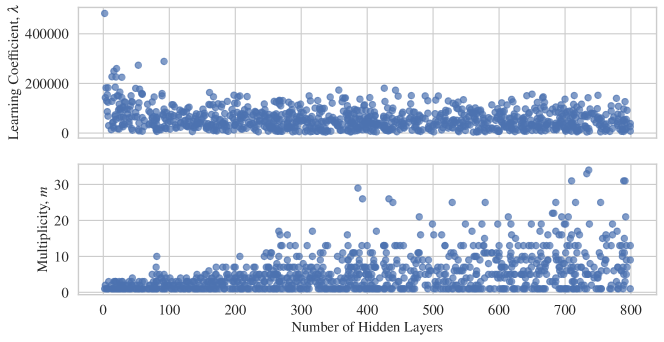
Figure 7: The top graph shows $\lambda$ decreasing as the DLN becomes deeper, even though model parameter count increases with number of layers. The bottom graph shows the true multiplicities, $m$. Since regular models can only have $m=1$, the graph shows that most of these randomly generated DLNs are singular.

Appendix C Model complexity vs model-independent complexity

In this paper, we have described the LLC as a measure of “model complexity.” It is worth clarifying what we mean here — or rather, what we do not mean.

We distinguish measures of “model complexity,” such as those traditionally found in statistical learning theory, from measures of “model-independent complexity,” such as those found in algorithmic information theory. Measures of model complexity, like the parameter count, describe the expressivity or degrees of freedom available to a particular model. Measures of model-independent complexity, like Kolmogorov complexity, describe the complexity inherent to the task itself.

In particular, we emphasize that — a priori — the LLC is a measure of model complexity, not model-independent complexity. It can be seen as the amount of information required to nudge a model towards $w^{*}$ and away from other parameters. Parameters with higher LLC are more complex for that particular model to implement.

Alternatively, the model is inductively biased towards parameters with lower LLC — but a different model could have different inductive biases, and thus different LLC for the same task. This is why it is not sensible to conclude that a bias towards low LLC, would, on its own, explain observed “simplicity bias” in neural networks Valle-Perez et al. (2018) — this is tautological.

To highlight this distinction, we construct a statistical model where these two notions of complexity diverge. Let $f_{1}(x)$ be a Kolmogorov-simple function, like the identity function. Let $f_{2}(x)$ be a Kolmogorov-complex function, like a random lookup table. Then consider the following regression model with a single parameter $w\in[0,1]$:

$$f(x,w)=w^{8}f_{1}(x)+(1-w^{8})f_{2}(x)$$

For this model, $f_{1}(x)$ has an learning coefficient of $\lambda=\frac{1}{2}$, whereas $f_{2}(x)$ has a learning coefficient of $\lambda=\frac{1}{16}$. Therefore, despite $f_{1}(w)$ being more Kolmogorov-simple, it is more complex for $f(x,w)$ to implement — the model is biased towards $f_{2}(w)$ instead of $f_{1}(w)$, and so $f_{1}(w)$ requires relatively more information to learn.

Yet, this example feels contrived: in realistic deep learning settings, the parameters $w$ do not merely interpolate between handpicked possible algorithms, but themselves define an internal algorithm based on their values. That is, it seems intuitively like the parameters play a role closer to “source code” than “tuning constants.”

Thus, while in general LLC is not a model-independent complexity measure, it seems distinctly possible that for neural networks (perhaps even models in some broader “universality class”), the LLC could be model-independent in some way. This would theoretically establish the inductive biases of neural networks. We believe this to be an intriguing direction for future work.

Appendix D Recommendations for accurate estimation

Much as in a field like experimental physics, we find that having theoretical values to compare against gives us strong feedback on our experimental procedures, which can then apply even when theoretical values are not available. Based on this experience, we have several recommendations for estimating the learning coefficient accurately in practice.

D.1 Step size

From experience, the most important hyperparameter to the performance and accuracy of the method is the step size $\epsilon$. If the step size is too low, the sampler may not equilibriate, leading to underestimation. If the step size is too high, the sampler can become numerically unstable, causing overestimation or even “blowing up” to NaN values.

Manual tuning of the step size is possible, but subjective and hard to fine-tune. Instead we strongly recommend a particular diagnostic based on the acceptance criterion for Metropolis-adjusted Langevin dynamics (MALA). This is used to correct numerical errors in traditional MCMC, but here we use it only to detect them.

In traditional (full-gradient) MCMC, numerical errors caused by the step size are completely corrected by a secondary step in the algorithm, the acceptance check or Metropolis correction, which accepts or rejects steps with some probability roughly based on the likelihood of numerical error. The proportion of steps accepted additionally becomes an important diagnostic as to the health of the algorithm: a low acceptance ratio indicates that the acceptance check is having to compensate for high levels of numerical error.

The acceptance probability between step $X_{k}$ and proposed step $X_{k+1}$ is calculated as:

$$\min\left(1,\frac{\pi(X_{k})\,q(X_{k}\mid X_{k+1})}{\pi(X_{k+1})\,q(X_{k+1}\mid X_{k})}\right)$$

where $\pi(x)$ is the probability density at $x$ (in our case, $\log\pi(x)=\beta nL_{n}(x)$), and $q(x^{\prime}\mid x)$ is the probability of our sampler transitioning from $x$ to $x^{\prime}$.

In the case of MALA, $q(x^{\prime}\mid x)\not=q(x\mid x^{\prime})$ and so we must explicitly calculate this term. For MALA, it is:

$$q(x^{\prime}\mid x)\propto\exp(-\frac{1}{4\epsilon}||x^{\prime}-x-\epsilon\nabla\log\pi(x)||^{2})$$

We choose to use MALA’s formula because we are using SGLD, and both MALA and SGLD propose steps using Langevin dynamics. MALA’s formula is the correct one to use when attempting to apply Metropolis correction to Langevin dynamics.

For various reasons, directly implementing such an acceptance check for stochastic-gradient MCMC (while possible) is typically either ineffective or inefficient. Instead we use the acceptance probability merely as a diagnostic.

We recommend tuning the step size such that the average acceptance probability is in the range of 0.9-0.95. Below this range, increase step size to avoid numerical error. Above this range, consider decreasing step size for computational efficiency (to save on the number of steps required). For efficiency, we recommend calculating the acceptance probability for only a fraction of steps — say, one out of every twenty.

Note that since we are not actually using an acceptance check, these acceptance “probabilities” are not really probabilities, but merely diagnostic values.

D.2 Step count and burn-in

The step count for sampling should be chosen such that the sampler has time to equilibriate or “burn in.” Insufficient step count may lead to underestimating the learning coefficient. Excessive step count will never degrade accuracy, but is unnecessarily time-consuming.

We recommend increasing the number of steps until the loss stops increasing after some period of time. This can be done with manual inspection of the loss trace. See Figure 8 for some examples of loss trace and MALA acceptance probability over SGLD trajectories for DLN model at different scale.

It is worth noting that the loss trace should truly be flat — a long, slow upwards slope can still be indicative of significant underestimation.

We also recommend that samples during this burn-in period are discarded. That is, loss values should only be tallied once they have flattened out. This avoids underestimation.

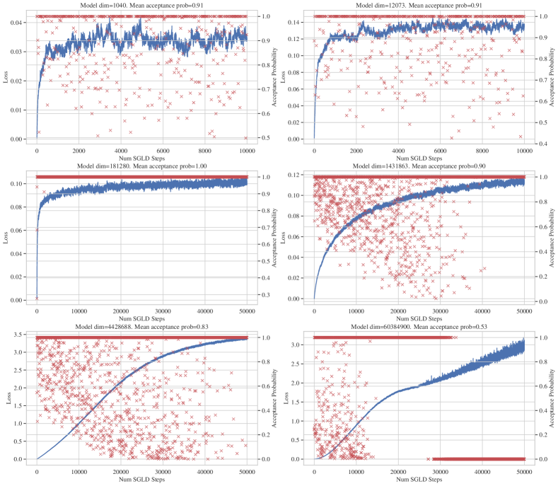
Figure 8: Sample loss trace and MALA acceptance probability over DLN training trajectories at different model sizes.

D.3 Scaling

We emphasize that hyperparameters must be tuned independently for different model sizes. In particular, the required step size for numerical stability tends to decrease for larger models, forcing a compensatory increase in the step count. See Table 1 for an example of this tuning with scale.

Future work using e.g. $\mu$-parameterization Yang et al. (2022) may be able to alleviate this issue.

Appendix E Additional experimental details

Experiments involving DLN are run on Nvidia A100 GPU while all other experiments are run on CPU.

E.1 Experiment: DLN $\hat{\lambda}(w^{*})$-vs-$\lambda$ experiments

As described in Section 4.2, the experiments shown in Figure 1 consist of randomly constructed DLN. For each target order of magnitude of DLN parameter count, we randomly sample the number of layers and their widths from a different range. We also use a different set of SGLD hyperparameter chosen according to the recommendation made in Section D. Configuration values that varies across OOM are shown in Table 1 and other configurations are as follow

• Batch size used in SGLD is 500.

• The amount of burn-in steps used for SGLD samples is set to 90% of total SGLD chain length, i.e. only the last 10% of SGLD samples are used in estimating the LLC.

• The quadratic confinement strength $\gamma$ is set to $1.0$.

• For each DLN, $f(x,w^{*})$ with a chosen true parameter $w^{*}$, a synthetic dataset, $\{(x_{i},y_{i})\}_{i=1,\dots,n}$ is generated by randomly sampling each element of the input vector $x$ uniformly from the interval $[-10,10]$ and set the output as $y=f(x,w^{*})$.

• For LLC estimation done at a trained parameter instead of the true parameter (shown in Figure 4), the network is first trained using SGD with learning rate 0.01 and momentum 0.9 for 50000 steps.

For each target OOM, a number of different experiments are run with different random seeds. The number of such experiment is determined by our compute resources and is reported in Table 1 with some experiment failing due to SGLD chains “blowing up” (See discussion in Appendix D) for the SGLD hyperparameters used. Figure 12 shows that there is a left tail to the mean MALA acceptance rate distribution that hint at instability in SGLD chains encountered in some $\hat{\lambda}(w^{*})$ estimation run.

OOM	Num layers	Widths	$\epsilon$	Num SGLD steps	$n$	Num experiments
1k	2-5	5-50	$5\times 10^{-7}$	10k	$10^{5}$	99
10k	2-10	5-100	$5\times 10^{-7}$	10k	$10^{5}$	100
100k	2-10	50-500	$1\times 10^{-7}$	50k	$10^{6}$	100
1M	5-20	100-1000	$5\times 10^{-8}$	50k	$10^{6}$	99
10M	2-20	500-2000	$2\times 10^{-8}$	50k	$10^{6}$	93
100M	2-40	500-3000	$2\times 10^{-8}$	50k	$10^{6}$	54

Table 1: Table of experimental configuration for each batch of experiment at different order of magnitudes (OOM) in DLN model size. $n$ denotes the training dataset size and $\epsilon$ denotes SGLD step size (See Section 3.2).

E.2 Experiment: Detecting saddle-to-saddle dynamics with LLC

As mentioned in the main text, the experimental setup is parallel to the experiments of Jacot et al. (2021). Specifically,

• Only “rectangular” DLN, those with constant hidden layer width $H$, are considered. The input and output dimension of the DLNs are fixed at $5$. In the notation of Equation 7, a DLN, $f(x,w)$ with $M$ hidden layers is specified by $(H_{0},H_{1},\dots,H_{M-1},H_{M})=(5,H,\dots,H,5)$.

• Training dataset of size $n=10000$ are created by generating random Gaussian input array $X$ of shape $n\times 5$ and pass through a fixed teacher DLN specified by the single matrix: $10\cdot\mathrm{diag}(1,2,3,4,5)$ forming a $n\times 5$ output array $Y$. No noise is added to the training data.

• The initial parameter of the a student DLN with $M$ hidden layers of constant width $H$ is drawn from a Gaussian distribution $N(0,\sigma^{2})$ with variance $\sigma^{2}=H^{-\delta}$. We set $\delta=1.5$ as per Jacot et al. (2021) to probe the “saddle-to-saddle” regime.

• The network is then trained using SGD with learning rate $\eta$ without momentum for $T$ iterations

• The configuration values $H$, $M$, $\eta$, $T$ are shown in the title of resulting graphs.

Over the course of training, we measure $\hat{\lambda}(w_{t})$ for every parameter encountered for every $k$ SGD iterations with SGLD hyperparameters (see Section 3.2) fixed to $\epsilon=10^{-6}$, $\gamma=1.0$, number of steps $=100$ and batch size $=128$.

Note that there is an important modification to the LLC estimation procedure for this experiment. Instead of using the training dataset $(X,Y)$ for SGLD sampling, we use the dataset $(X,f(X,w_{t}))$ to estimate $\hat{\lambda}(w_{t})$ at parameter $w_{t}$. Conceptually, this is equivalent to treating the DLN as a statistical model at parameter $w_{t}$ as the true data generating distribution, ensuring realizability and that $w_{t}$ being a global minimum of the loss function.

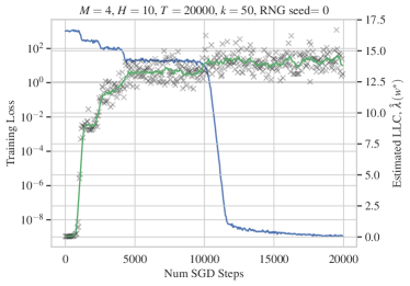
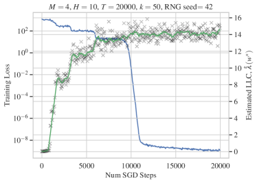
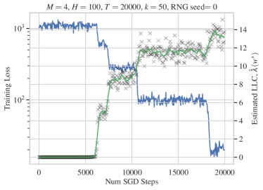
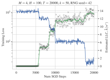
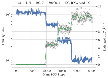
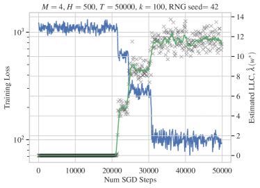
Figure 9: Additional runs similar to Figure 5. $\hat{\lambda}(w^{*})$ detects changes to the local geometry of DLN loss landscapes over the course of training. Each plot title records the experiment configuration with variable names explained in Appendix E.2

E.3 Additional plots for DLN experiments

• Figure 10 is a linear scale version of Figure 1 in the main text. This shows the estimated LLC against the true learning coefficients for experiments at different model size range without log-scale distortion.

• Figure 11 shows the relative error $(\lambda-\hat{\lambda}(w^{*}))/\lambda$ across multiple orders of magnitude of DLN model size.

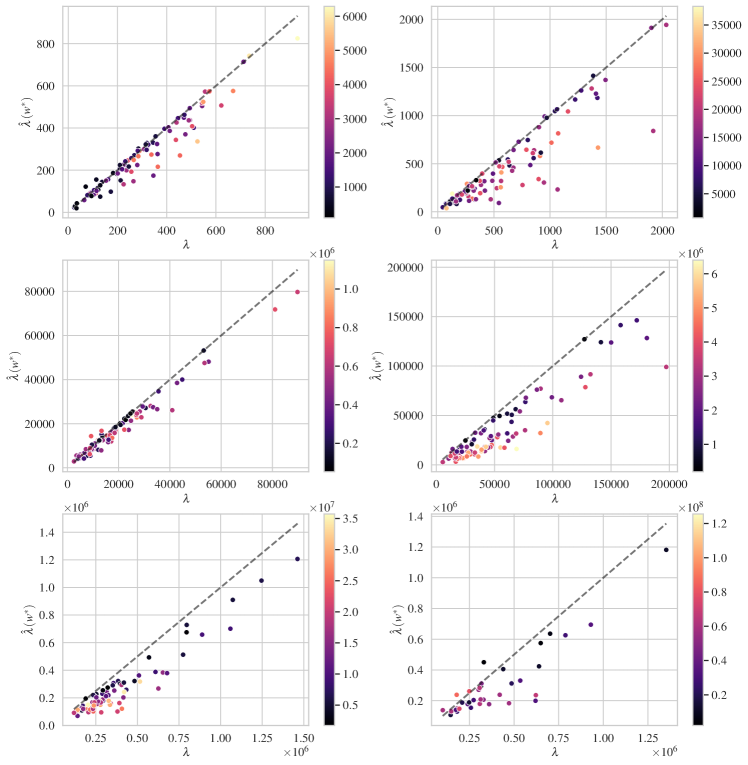
Figure 10: Supplementary plot to Figure 1. Each plot shows a single batch of DLN experiment with model size at different order of magnitude. The SGLD hyperparameter is tuned once for each batch. Their values are listed in Table 1 In contrast to Figure 1 which is in log scale, all plots here are in linear scale.

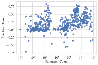
Figure 11: Relative error of estimated LLC compared to the theoretical learning coefficient, for DLNs across different orders of magnitude of model size.

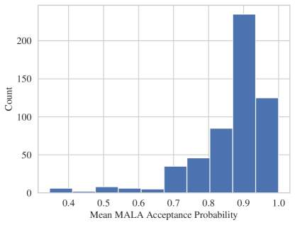
Figure 12: Mean MALA acceptance probability over the entire SGLD trajectory for every DLN experiment. Model size is not the only factor affecting the correct scale for SGLD step size. Local geometry varies significantly among different models, and among different neighbourhoods in the parameter space. Without tuning SGLD hyperparameters individually for each experiment, we get a spread of (mean) MALA acceptance probability over all experiments. Those with low acceptance probability may indicate poor $\hat{\lambda}(w^{*})$ estimation quality.

References

- Aoyagi (2024) Aoyagi, M. Consideration on the learning efficiency of multiple-layered neural networks with linear units. Neural Networks, pp. 106132, 2024.
- Aoyagi et al. (2005) Aoyagi, M., Watanabe, S., et al. Resolution of singularities and the generalization error with Bayesian estimation for layered neural network. IEICE Trans, 88(10):2112–2124, 2005.
- Arora et al. (2018) Arora, S., Cohen, N., Golowich, N., and Hu, W. A convergence analysis of gradient descent for deep linear neural networks. arXiv preprint arXiv:1810.02281, 2018.
- Ashcroft & Mermin (2022) Ashcroft, N. W. and Mermin, N. D. Solid State Physics. Cengage Learning, 2022.
- Berner et al. (2019) Berner, J., Elbrächter, D., and Grohs, P. How degenerate is the parametrization of neural networks with the ReLU activation function? In Neural Information Processing Systems, 2019.
- Blalock et al. (2020) Blalock, D., Gonzalez Ortiz, J. J., Frankle, J., and Guttag, J. What is the state of neural network pruning? Proceedings of Machine Learning and Systems, 2:129–146, 2020.
- Chen et al. (2023) Chen, Z., Lau, E., Mendel, J., Wei, S., and Murfet, D. Dynamical versus Bayesian phase transitions in a toy model of superposition, 2023.
- Dinh et al. (2017) Dinh, L., Pascanu, R., Bengio, S., and Bengio, Y. Sharp minima can generalize for deep nets. In International Conference on Machine Learning, pp. 1019–1028. PMLR, 2017.
- Endo et al. (2020) Endo, A., Abbott, S., Kucharski, A. J., Funk, S., et al. Estimating the overdispersion in COVID-19 transmission using outbreak sizes outside China. Wellcome Open Research, 5, 2020.
- Farrugia-Roberts (2023) Farrugia-Roberts, M. Functional equivalence and path connectivity of reducible hyperbolic tangent networks. In Thirty-seventh Conference on Neural Information Processing Systems, 2023.
- Fefferman (1994) Fefferman, C. Reconstructing a neural net from its output. Revista Matemática Iberoamericana, 10(3):507–555, 1994.
- Fontanesi et al. (2019) Fontanesi, L., Gluth, S., Spektor, M. S., and Rieskamp, J. A reinforcement learning diffusion decision model for value-based decisions. Psychonomic Bulletin & Review, 26(4):1099–1121, 2019.
- Fukumizu (1996) Fukumizu, K. A regularity condition of the information matrix of a multilayer perceptron network. Neural Networks, 9(5):871–879, 1996.
- Grünwald & Roos (2019) Grünwald, P. and Roos, T. Minimum description length revisited. International journal of mathematics for industry, 11(01):1930001, 2019.
- Haario et al. (1999) Haario, H., Saksman, E., and Tamminen, J. Adaptive proposal distribution for random walk Metropolis algorithm. Computational Statistics, 14:375–395, 1999.
- Haario et al. (2001) Haario, H., Saksman, E., and Tamminen, J. An adaptive metropolis algorithm. Bernoulli, pp. 223–242, 2001.
- Hinton et al. (2015) Hinton, G., Vinyals, O., and Dean, J. Distilling the knowledge in a neural network. arXiv preprint arXiv:1503.02531, 2015.
- Hochreiter & Schmidhuber (1997) Hochreiter, S. and Schmidhuber, J. Flat Minima. Neural Computation, 9(1):1–42, 01 1997. ISSN 0899-7667. doi: 10.1162/neco.1997.9.1.1. URL https://doi.org/10.1162/neco.1997.9.1.1.
- Hoogland & Van Wingerden (2023) Hoogland, J. and Van Wingerden, S. You’re measuring model complexity wrong, Oct 2023. URL https://www.alignmentforum.org/posts/6g8cAftfQufLmFDYT/.
- Hoogland et al. (2024) Hoogland, J., Wang, G., Farrugia-Roberts, M., Carroll, L., Wei, S., and Murfet, D. The developmental landscape of in-context learning. In preparation, 2024.
- Hooten & Hobbs (2015) Hooten, M. B. and Hobbs, N. T. A guide to Bayesian model selection for ecologists. Ecological Monographs, 85(1):3–28, 2015.
- Imai (2019a) Imai, T. Estimating real log canonical thresholds. arXiv preprint arXiv:1906.01341, 2019a.
- Imai (2019b) Imai, T. On the overestimation of widely applicable Bayesian information criterion. arXiv preprint arXiv:1908.10572, 2019b.
- Iriguchi & Watanabe (2007) Iriguchi, R. and Watanabe, S. Estimation of poles of zeta function in learning theory using Padé approximation. In Artificial Neural Networks–ICANN 2007: 17th International Conference, Porto, Portugal, September 9-13, 2007, Proceedings, Part I 17, pp. 88–97. Springer, 2007.
- Jacot et al. (2021) Jacot, A., Ged, F., Şimşek, B., Hongler, C., and Gabriel, F. Saddle-to-Saddle dynamics in deep linear networks: Small initialization training, symmetry, and sparsity. June 2021.
- Ji & Telgarsky (2018) Ji, Z. and Telgarsky, M. Gradient descent aligns the layers of deep linear networks. arXiv preprint arXiv:1810.02032, 2018.
- Jiang et al. (2019) Jiang, Y., Neyshabur, B., Mobahi, H., Krishnan, D., and Bengio, S. Fantastic generalization measures and where to find them, 2019.
- Jules et al. (2023) Jules, T., Brener, G., Kachman, T., Levi, N., and Bar-Sinai, Y. Charting the topography of the neural network landscape with thermal-like noise, 2023.
- Kafashan et al. (2021) Kafashan, M., Jaffe, A. W., Chettih, S. N., Nogueira, R., Arandia-Romero, I., Harvey, C. D., Moreno-Bote, R., and Drugowitsch, J. Scaling of sensory information in large neural populations shows signatures of information-limiting correlations. Nature Communications, 12(1):473, 2021.
- Kůrková & Kainen (1994) Kůrková, V. and Kainen, P. C. Functionally equivalent feedforward neural networks. Neural Computation, 6:543–558, 1994.
- LaMont & Wiggins (2019) LaMont, C. H. and Wiggins, P. A. Correspondence between thermodynamics and inference. Physical Review E, 99(5), May 2019. ISSN 2470-0053. doi: 10.1103/physreve.99.052140. URL http://dx.doi.org/10.1103/PhysRevE.99.052140.
- Lau et al. (2023) Lau, E., Murfet, D., and Wei, S. Quantifying degeneracy in singular models via the learning coefficient. 2023. doi: 10.48550/arXiv.2308.12108. URL http://arxiv.org/abs/2308.12108.
- Petersen et al. (2020) Petersen, P. C., Raslan, M., and Voigtlaender, F. Topological properties of the set of functions generated by neural networks of fixed size. Foundations of Computational Mathematics, 21:375 – 444, 2020.
- Phuong & Lampert (2020) Phuong, M. and Lampert, C. H. Functional vs. parametric equivalence of ReLU networks. In International Conference on Learning Representations, 2020.
- Roberts & Rosenthal (1998) Roberts, G. O. and Rosenthal, J. S. Optimal scaling of discrete approximations to Langevin diffusions. Journal of the Royal Statistical Society: Series B (Statistical Methodology), 60(1):255–268, 1998.
- Saxe et al. (2013) Saxe, A. M., McClelland, J. L., and Ganguli, S. Exact solutions to the nonlinear dynamics of learning in deep linear neural networks. arXiv preprint arXiv:1312.6120, 2013.
- Semenova et al. (2020) Semenova, E., Williams, D. P., Afzal, A. M., and Lazic, S. E. A Bayesian neural network for toxicity prediction. Computational Toxicology, 16:100133, 2020.
- Sharma (2017) Sharma, S. Markov chain Monte Carlo methods for Bayesian data analysis in astronomy. Annual Review of Astronomy and Astrophysics, 55:213–259, 2017.
- Sussmann (1992) Sussmann, H. J. Uniqueness of the weights for minimal feedforward nets with a given input-output map. Neural Networks, 5(4):589–593, 1992.
- Valle-Perez et al. (2018) Valle-Perez, G., Camargo, C. Q., and Louis, A. A. Deep learning generalizes because the parameter-function map is biased towards simple functions. arXiv preprint arXiv:1805.08522, 2018.
- Watanabe (2001) Watanabe, S. Algebraic analysis for nonidentifiable learning machines. Neural Computation, 13(4):899–933, 2001.
- Watanabe (2007) Watanabe, S. Almost all learning machines are singular. In 2007 IEEE Symposium on Foundations of Computational Intelligence, pp. 383–388. IEEE, 2007.
- Watanabe (2009) Watanabe, S. Algebraic Geometry and Statistical Learning Theory. Cambridge University Press, 2009.
- Watanabe (2010) Watanabe, S. Asymptotic learning curve and renormalizable condition in statistical learning theory. Journal of Physics: Conference Series, 233:012014, June 2010.
- Watanabe (2013) Watanabe, S. A widely applicable bayesian information criterion. Journal of Machine Learning Research, 14(27):867–897, 2013. URL http://jmlr.org/papers/v14/watanabe13a.html.
- Watanabe (2018) Watanabe, S. Mathematical theory of Bayesian statistics. CRC Press, 2018.
- Wei et al. (2022) Wei, S., Murfet, D., Gong, M., Li, H., Gell-Redman, J., and Quella, T. Deep learning is singular, and that’s good. IEEE Transactions on Neural Networks and Learning Systems, 2022.
- Welling & Teh (2011) Welling, M. and Teh, Y. W. Bayesian learning via stochastic gradient Langevin dynamics. In Proceedings of the 28th International Conference on Machine Learning (ICML-11), pp. 681–688, 2011.
- Yamazaki & Watanabe (2003) Yamazaki, K. and Watanabe, S. Singularities in mixture models and upper bounds of stochastic complexity. Neural Networks, 16(7):1029–1038, 2003.
- Yamazaki & Watanabe (2005a) Yamazaki, K. and Watanabe, S. Singularities in complete bipartite graph-type Boltzmann machines and upper bounds of stochastic complexities. IEEE transactions on neural networks, 16(2):312–324, 2005a.
- Yamazaki & Watanabe (2005b) Yamazaki, K. and Watanabe, S. Algebraic geometry and stochastic complexity of hidden Markov models. Neurocomputing, 69(1-3):62–84, 2005b.
- Yang et al. (2022) Yang, G., Hu, E. J., Babuschkin, I., Sidor, S., Liu, X., Farhi, D., Ryder, N., Pachocki, J., Chen, W., and Gao, J. Tensor programs V: Tuning large neural networks via zero-shot hyperparameter transfer. arXiv preprint arXiv:2203.03466, 2022.
- Zhang et al. (2017) Zhang, C., Bengio, S., Hardt, M., Recht, B., and Vinyals, O. Understanding deep learning requires rethinking generalization, 2017.
- Zhang et al. (2018) Zhang, Y., Saxe, A. M., Advani, M. S., and Lee, A. A. Energy–entropy competition and the effectiveness of stochastic gradient descent in machine learning. Molecular Physics, 116(21–22):3214–3223, June 2018. ISSN 1362-3028. doi: 10.1080/00268976.2018.1483535. URL http://dx.doi.org/10.1080/00268976.2018.1483535.