ServeFlow: A Fast-Slow Model Architecture for Network Traffic Analysis

Abstract.

Network traffic analysis increasingly uses complex machine learning models as the internet consolidates and traffic gets more encrypted. However, over high-bandwidth networks, flows can easily arrive faster than model inference rates. The temporal nature of network flows limits simple scale-out approaches leveraged in other high-traffic machine learning applications. Accordingly, this paper presents ServeFlow, a solution for machine-learning model serving aimed at network traffic analysis tasks, which carefully selects the number of packets to collect and the models to apply for individual flows to achieve a balance between minimal latency, high service rate, and high accuracy. We identify that on the same task, inference time across models can differ by 2.7x–136.3x, while the median inter-packet waiting time is often 6–8 orders of magnitude higher than the inference time! ServeFlow is able to make inferences on 76.3% flows in under 16ms, which is a speed-up of 40.5x on the median end-to-end serving latency while increasing the service rate and maintaining similar accuracy. Even with thousands of features per flow, it achieves a service rate of over 48.5k new flows per second on a 16-core CPU commodity server, which matches the order of magnitude of flow rates observed on city-level network backbones.

1. Introduction

Data-driven models from machine learning (ML) have the potential to enhance the performance (Lotfollahi et al., 2020; Zheng et al., 2022; Rimmer et al., 2017; Bronzino et al., 2021; Jiang et al., 2023c), observability (Liu et al., 2023a, b; Sharma et al., 2023; MacMillan et al., 2021; Piet et al., 2023), and security of networks (Holland et al., 2021a; Jiang et al., 2023b, a). Many of the applications of these models are for network traffic analysis tasks, such as service recognition (Bernaille et al., 2006; Shapira and Shavitt, 2021; Rezaei et al., 2019; Jiang et al., 2023c), quality of experience (QoE) measurement on encrypted traffic (Mangla et al., 2018; Bronzino et al., 2019; Sharma et al., 2023), intrusion detection (Khraisat et al., 2019; Ahmad et al., 2021; Liu and Lang, 2019) and device identification (Yang et al., [n. d.]; Sivanathan et al., 2019). The goal of these tasks is to classify network traffic flows into discrete categories that characterize these flows. These classifications are often used for traffic management, which requires fast reaction times. For example, for flow prioritization and QoE control, service recognition, and QoE measurement need to happen in real time with a latency requirement of under 50ms (Staessens et al., 2011). For network intrusion detection, decisions need to be made as fast as possible to prevent damage (Ahmad et al., 2021; Mittal et al., 2023). Although ML-based approaches have been shown to be far more accurate and robust than simple heuristics (e.g., based on TCP/UDP port numbers), it can be challenging to deploy such systems in high-bandwidth networks. The model evaluation either needs to be faster than the incoming network traffic or sufficiently parallelized so that multiple network flows can be classified simultaneously.

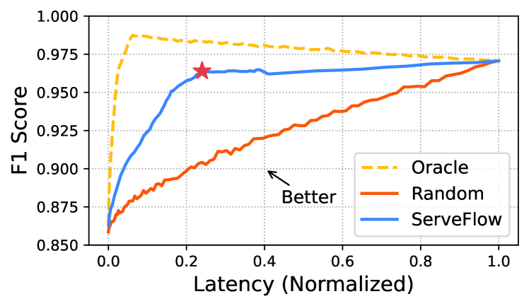
Figure 1. There is a natural tradeoff between latency and accuracy. ServeFlow intelligently reassigns predictions to a slow and more accurate model (waits for more packets as features or a more sophisticated design) or to a fast but less accurate model (most efficient and makes predictions on the first packet). The chart shows the efficacy of the request assignment algorithm compared to an oracle that assigns models based on ground-truth knowledge on the correctness of classification, and a random assignment.

To understand these deployment bottlenecks, consider a typical network classification workflow (Fig. 2). First, a packet-capturing framework collects and segments active network flows (data collection). Next, these flows are converted into numerical features (featurization). These features are inputs to the model which returns a classification result (inference). In many ML problems, the primary bottleneck is the inference step. There are many techniques to improve the latency of model inference, such as model pruning and quantization (Liu et al., 2018; Fang et al., 2023; Fan et al., 2020), knowledge distillation (Wang and Yoon, 2021; Gou et al., 2021), hardware acceleration (Ghimire et al., 2022), data compression (Yang et al., 2020; Hu and Krishnamachari, 2020), and model specialization (Li et al., 2021; Hu et al., 2021). Accordingly, there are several approaches applied to networking problems including: efficient modeling (Piet et al., 2023; Koksal et al., 2022; Qiu et al., 2022; Tong et al., 2014; Devprasad et al., 2022; Liu et al., 2019), feature selection (Bronzino et al., 2021; Jiang et al., 2023c), and specialized hardware (like SmartNICs) (e.g., N3IC (Siracusano et al., 2022), Homunculus (Swamy et al., 2023), and Taurus (Swamy et al., 2022)). However, simply reducing the latency of featurization and model inference, may not sufficiently improve the performance of the overall system. The initial data collection step can contribute orders of magnitude more hidden latency in network classifications.

For most practical use cases, the classifier needs to be able to issue a traffic classification while a flow is active so the system can act on this result (e.g., change flow priority or reject malicious flows). However, the model must wait for sufficient information from a flow to arrive before doing any further processing. Waiting longer gives the model more context on a flow, and thus, a more accurate final result (Bernaille et al., 2006; Piet et al., 2023). Conventional flow-level classification methods typically wait between 4 and 100 packets (Holland et al., 2021a; Piet et al., 2023; Jiang et al., 2023c), while others demand the entire flow (Shapira and Shavitt, 2021; Bronzino et al., 2019; Sharma et al., 2023). For example, a recent high-performance method GGFAST (Piet et al., 2023) needs to wait for 50 packets to craft informative sequence-of-lengths features. Waiting for packets from a particular flow to arrive is a form of model latency. It requires a dedicated system thread to query the network capture stream which reduces the overall throughput of a classification system.

Although this gap in data collection time might seem like a fundamental technical bottleneck, this paper contributes a key insight into many network traffic classification problems: some flows are easy to classify, and some are harder. For example, for the first packet, a typical web browsing request may display standard TCP options like MSS, Window Scale, and SACK, while specialized applications or services like VPNs or database query protocols often exhibit unique or rare TCP options. In these cases, it is possible to accurately classify some traffic with a single packet. To exploit this skew, we develop a new model inference architecture that ensembles information arriving at different time points from multiple different models. Instead of using a single conventional “slow” (requires long flow context but is more accurate) model, we place additional “fast” (requires less flow context) models in front of it. This architecture can balance accuracy with waiting time (i.e., return a less accurate answer earlier). A selection algorithm assigns uncertain predictions from the fast model for further processing on the slow model. We present a novel message-queuing architecture that efficiently and coherently maintains network flow state. This fast-slow architecture is especially beneficial when the two models involved have high disparities in their performance and operational cost. Figure 1 illustrates the basic results, showing that ServeFlow presents the user with a latency-accuracy tradeoff rather than a single design point.

Ethics: This work does not raise any ethical issues.

2. Background and Motivation

Next, we describe the functionality of existing systems and why they are insufficient for network traffic analysis.

Figure 2. Networking ML pipeline.

Application	Model	F1 (1pkt)	F1(5pkts)	F1(10pkts)
	DT	$0.845$	$0.907$	$0.909$
Service Rec.	LGBM	$0.921$	$0.967$	$0.973$
	CNN	$0.887$	$0.929$	$0.930$
	DT	$0.812$	$0.824$	$0.827$
Device Id.	LGBM	$0.913$	$0.918$	$0.919$
	CNN	$0.881$	$0.910$	$0.911$
	DT	$0.715$	$0.740$	$0.745$
VCA QoE	LGBM	$0.723$	$0.769$	$0.773$
	CNN	$0.710$	$0.752$	$0.764$

Table 1. Empirically, adding more packets increases the classification (weighted) F1 score.

2.1. Model Serving Systems

Serving trained ML models is an important part of any ML task. Model serving systems, such as TensorFlow Serving (Olston et al., 2017) and TorchServe (Paszke et al., 2019), provide service interfaces to trained models. These systems are designed for scaling out in the cloud and prioritize “parallelism through asynchrony”, i.e., each inference request is independent and can be served by a pool of threads. Many model-serving frameworks (e.g., Clipper (Crankshaw et al., 2017), InferLine (Crankshaw et al., 2020)) leverage a large number of parallel workers to improve overall system throughput. When inference requests are independent of each other, such a stateless-parallelism approach is straightforward. However, the streaming nature of network traffic means that each individual packet is potentially coupled with previously seen packets. Thus, in the network setting, there is additional state management needed to understand where in a flow a packet is coming from. Moreover, traffic volume could surpass the maximum capacity of all workers. In such cases, it is essential to develop systems that are capable of intelligently prioritizing network flows, especially under resource saturation. For these reasons, we develop ServeFlow, a new model serving framework aimed at networking problems.

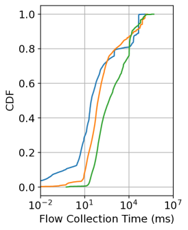
(a)

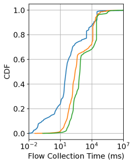
(b)

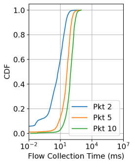
(c)

Figure 3. Flow collection time (since the arrival of the first packet, in ms) across applications. Note that some flows do not have five (or more) packets, so at the tail, flow collection time would be smaller compared to collecting two packets.

Application	Model	1 Pkt	5 Pkts	10 Pkts
Feature Computation Time		0.012	0.058	0.139
	DT	0.052	0.142	0.251
Service Rec.	LGBM	0.139	0.237	0.358
	CNN	0.481	3.815	7.345
	DT	0.053	0.145	0.275
Device Id.	LGBM	0.210	0.322	0.460
	CNN	0.491	3.277	6.446
	DT	0.053	0.095	0.164
VCA QoE	LGBM	0.162	0.218	0.298
	CNN	0.385	3.290	6.543

Table 2. Median feature compute time, and median inference time (both in ms) for different models. DT: Decision Tree, LGBM: LightGBM, CNN: Convolutional Neural Networks.

2.2. Machine Learning for Networking

Many machine learning for networking problems are designed for the offline setting, where models are applied to previously collected flows. Thus, such methods require the observation of 4 to 100 packets to even the entire flow for effective classification (Holland et al., 2021a; Piet et al., 2023; Jiang et al., 2023c; Shapira and Shavitt, 2021; Bronzino et al., 2019; Sharma et al., 2023). In the online setting, waiting to buffer packets from a flow can add prohibitive latency to an ML-based networking component.

There are two key tradeoffs at play here. First, longer context lengths (i.e., observing more data for a given flow), typically result in more accurate models but have higher end-to-end latency. This latency comes from both waiting time and additional feature processing time. Next, more expressive models can be more accurate but have larger inference latencies and may require more computing resources such as memory or specialized hardware.

Table 1 puts these tradeoffs into perspective. It shows the F1 score as a function of context size for several different widely used models (Lotfollahi et al., 2020; Tong et al., 2014; Devprasad et al., 2022; Holland et al., 2021a; Liu et al., 2023b) and three different inference tasks (detailed in Sec. 5.1). The accuracy increases as we increase the context. However, for online classification, we would have to wait for those packets before any prediction. Figure 3 shows the CDF of waiting times for these packets. Larger contexts are more sensitive to network delays and jitter, which affect end-to-end decision latency.

Contrast the flow collection latency with the latency of model inference (Table 3). An example of a networking application would be an intrusion detection system. This system needs to analyze network packets in real time to detect possible threats. For each example task, we measure the latency of model inference with one packet of data context. Comparing Table 3 with Figure 3, we can see that the model inference latency is orders of magnitude smaller than the waiting time even for highly complex models. Furthermore, model inference latency is more predictable as it often derives from dense linear algebra operations with minimal control flow.

	Service Rec.		Device Id.		VCA QoE
Model	F1	Inf. Time	F1	Inf. Time	F1	Inf. Time
DT	0.845	0.052	0.812	0.053	0.715	0.053
RF	0.859	0.107	0.874	0.106	0.709	0.098
LGBM	0.921	0.139	0.913	0.210	0.723	0.162
XGB	0.672	0.117	0.507	0.152	0.646	0.127
CNN	0.887	0.481	0.881	0.491	0.710	0.385

Table 3. Different model performance for the 1st packet. Deeper green means higher F1 score, and deeper blue means lower model inference latency (in ms).

The primary goal of ServeFlow is to enhance performance by reducing inference latency while preserving the accuracy of its predictions. In this section, we delve deep into the intricacies of ServeFlow’s design, delineating its unique strategies to (1) apply a novel fast-slow serving architecture on both partial data (specifically, the first packet of a network flow) and how to use this partial data (by carefully choosing the model); (2) design a mechanism for assigning flow classification requests to different models; and (3) fully leverage diverse resources available in heterogeneous hardware environments.

3. Fast-slow Modeling

In this section, we explore the rationale and requirements for a fast-slow architecture, introducing ServeFlow which optimizes network traffic analysis through this concept. The key to this architecture is an algorithm developed to effectively differentiate between correct and incorrect predictions. We detail two designs in this section.

3.1. Fast-Slow Model Architecture

In any network classification problem that operates on flows, the amount of context provided to the model is a key parameter, namely, how much of the flow can the model see before making a decision. In prior work, this has been treated as a fixed hyper-parameter, but we find that varying this information to influence the responsiveness of the system is valuable. For instance, service recognition models can learn the service categorization of a flow using only the TCP options in the first packet (Holland et al., 2021a). Some categorizations may need more information to distinguish. They need inter-arrival time, sequences of packet sizes, or other flow-level features to provide more context. For example, QoE measurement on encrypted traffic needs more packets from the same session to understand rebuffering ratio (Mangla et al., 2018) or frame rates (Sharma et al., 2023).

Why might a fast-slow architecture be beneficial?

Taking advantage of the inherently discrete arrival of these packets, we have designed a fast-slow architecture for traffic analysis. This architecture enables inference based on partial flow information (i.e., incomplete context), addressing the varying demands for speed and accuracy. While slow models typically yield more accurate predictions, their reliance on the accumulation of a larger number of packets or on extensive computation makes them time-intensive. Conversely, a fast model offers rapid, albeit less accurate, predictions. Acting as a “filter”, the fast model initially processes all traffic, forwarding only those flows that necessitate higher accuracy to the slower, more meticulous models. For those satisfactory predictions made by the fast model, the latency is reduced by a large margin because it avoids waiting for more packets to come or more inference time.

When would a fast-slow architecture be beneficial?

Fast-slow modeling becomes particularly beneficial in scenarios where there is a significant disparity in operational costs between the fast and slow models. This encompasses factors such as data collection delays, featurization costs, state information tracking, and computational or memory demands for inference. Additionally, it also requires a sufficient difference in model performance: in some instances, even a fast model can meet the accuracy requirements for certain classes, which makes a slow model unnecessary. For many ML tasks, the complexity of a model often highly correlates with its operational cost, and it can also be a tentative indicator of the model’s performance. Thus, it forms an interesting search space for efficiency improvements.

How might the fast-slow model architecture generalize?

As discussed above: for the same task, if two models share disparities across their costs and performances, a fast-slow architecture could apply. For example, in network traffic analysis, two such opportunities exist: Firstly, packet waiting time often exceeds model inference time by several orders of magnitude, creating a natural disparity in latency. Secondly, the time taken for inference across identical inputs (whether partial or full) can also vary greatly, sometimes by 10x or more. This understanding opens the door to potentially even more nuanced applications of the architecture. For instance, a multi-tiered fast-slow approach could be implemented, where adjustments are made between each packet arrival (considering that packet inter-arrival times often surpass model inference times) or for different models at each packet number threshold. The challenge is ensuring that the time saved outweighs any added management overhead.

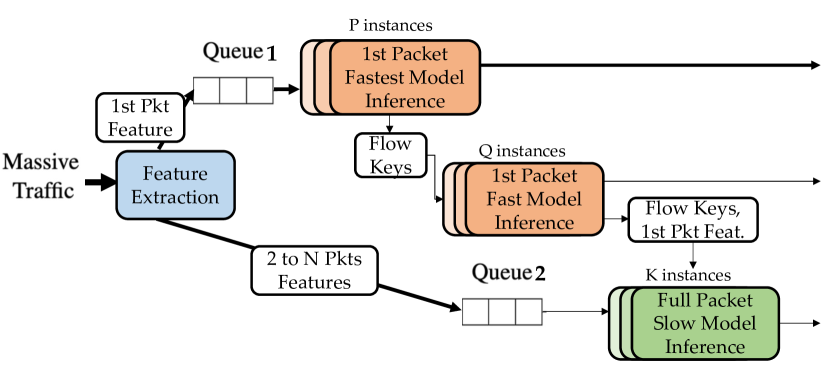
Figure 4. ServeFlow, which supports a novel fast-slow model serving pipeline, tailored to the discretely arriving packet nature of network flows. The width of arrows shows the portion of flows being processed at different stages.

We propose ServeFlow, where we capitalize on these two optimization avenues: the number of early-stage packets and the choice of model. As depicted in Figure 4, the “fastest” and “fast” model both use features from only the first packet, and the “slow” model uses more packets as input. Upon a flow’s entry into the network, the first packet is converted into an nPrint feature representation (Holland et al., 2021a), which effectively embeds information of all the raw header field bits. It is then sent to Queue 1 for immediate processing by the fastest inference model. This stage quickly filters through the traffic, identifying flows that are potentially misclassified. Should the fastest model’s predictions be deemed insufficient, the same initial packet features are subsequently analyzed by the fast model. This assesses whether a full packet inspection is necessary, offering a more refined evaluation without significantly compromising on speed. The fastest model, typically several times quicker than the fast model, significantly enhances throughput and reduces latency. Meanwhile, features from subsequent packets are accumulated in Queue 2. The slow model, upon a prompt from the fast model, combines these features with the initial packet’s data to perform inference. This asynchronously paced approach effectively balances the trade-off between speed and accuracy, ensuring quick response times for initial traffic assessment and detailed analysis for assigned classification requests. Note that not all ServeFlow applications have a fastest-fast-slow architecture, as the operational cost and performance gap might not be large enough on one of the dimensions.

Determining the placement of models within ServeFlow involves striking a balance between speed and performance. The ideal configuration places the fastest model at the entry of the network to evaluate the initial packet of each flow, provided that its performance is acceptable. This setup enables the system to make the quickest possible inferences. Conversely, at the other end of the spectrum, the system benefits from deploying the model with the best F1 score, fine-tuned with an optimally configured packet number (N), to function as the slow model for further analysis. To configure the fast model, the system requires a simple compilation and validation set testing, ensuring it delivers reliable performance by effectively filtering the classification requests.

3.2. Flow Assignment Algorithm

Assigning all flow classification requests to a slow model is not a good idea, not only because it harms the latency, but also because that there’s a risk of the slow model making erroneous corrections, which can further degrade performance. Surprisingly, even if one were to perfectly predict the correctness of these predictions (akin to having an “oracle”), this approach might still negatively affect the overall predictive performance as more requests are assigned to the slow model. This counterintuitive outcome is illustrated in Figure 1, which necessitates us to find a good assignment mechanism to balance the assigned portion with the F1 score.

We essentially need to evaluate the predictions made by the fastest or fast model, ServeFlow evaluates the likelihood of this prediction being “good enough”. This evaluation is crucial to determine whether the classification request of this flow should continue to the slower, more computationally intensive processing or if the prediction from the fastest or fast model suffices.

The core of ServeFlow’s efficiency lies in its assignment algorithm, which discerns the correctness of predictions made by the faster model. This algorithm is crafted to strategically assign subsets of data based on the uncertainty of their predictions. Specifically, this uncertainty is quantified using measures such as least confidence $LC(x)=1-\max\limits_{y}P(y|x)$, where $P(y|x)$ is the probability of the predicted label $y$, or entropy $H(x)=-\sum_{i}P(y_{i}|x)\log P(y_{i}|x)$, which accounts for the unpredictability inherent in the probability distribution of the predictions. These metrics, traditionally associated with sample selection for labeling during the training phase  (Liu et al., 2023b; Settles, 2009) — are adeptly repurposed in ServeFlow for inference use within its fast-slow serving architecture.

This assessment is anchored on the use of universal uncertainty thresholds. Algorithm 1 describes the process of setting this threshold. Given a validation set $D$, it computes the uncertainty for each data point in a given dataset, the algorithm constructs an uncertainty list. The list is then ordered, and a quantile value is set to determine the threshold.

Algorithm 1 Universal Uncertainty Threshold

function GetUniversalThreshold($D$)

    Initialize Uncertainty List $U$

    for each $DataPoint$ in Dataset $D$ do

        Compute Uncertainty $u$ for $DataPoint$

        Append $u$ to $U$

    end for

    Sort $U$ in ascending order

    Define Quantile Value $Q$

    Compute Quantile Index $qIndex\leftarrow\lceil Q\times\text{length of }U\rceil$

    Determine Threshold $T\leftarrow U[qIndex]$

    return Threshold $T$

end function

In contrast to a universal threshold, ServeFlow can also employ a more nuanced, class-specific approach as described in Algorithm 2. This approach recognizes that different classes may have varying levels of prediction certainty and, as such, different thresholds. The algorithm first segregates the dataset into correct and incorrect predictions per class label. It then establishes uncertainty thresholds for each class by examining the quantiles of uncertainty values. The key step involves calculating the assigned portions for correct and incorrect predictions at each threshold and using this information to determine the optimal slope for the assignment. This slope, a ratio of incorrectly assigned predictions to the total assigned, guides the setting of class-specific thresholds. The algorithm thus dynamically adjusts the uncertainty threshold for each class, tailoring the assignment process to improve the system’s overall predictive reliability and efficiency.

Algorithm 2 Slope-based Per-Class Uncertainty Thresholds

function GetPerClassThresholds($D,U$)

    Initialize Results $R$

    for each $ClassLabel$ in Dataset $D$ do

        Separate $D$ into Correct $C$ and Incorrect $I$ for $ClassLabel$

        if $I$ is empty then

           Store max uncertainty $U$ for $ClassLabel$ in $R$

        else

           Determine Thresholds $T$ from $U$ quantiles for $ClassLabel$

           Calculate assigned portions for $I$ and $C$ at each threshold

           Update $R$ with stats for each threshold

        end if

    end for

    Sort $R$ by assigned portions

    Calculate slope as $\frac{\Delta AssignedIncorrect}{\Delta AssignedAll}$ for each class

    Initialize Thresholds Dictionary $TD$ with the max $U$ for each class

    Set $AllAssigned$ to 0

    for each increment do

        if $AllAssigned<increment$ then

           Initialize MaxSlopeQueue $MSQ$

           Add top item of each class from $R$ to $MSQ$

           if $MSQ$ is empty then

               break

           end if

           Select item with max slope from $MSQ$

           Update $TD$ with this threshold

           Remove selected item from $R$

           Update $AllAssigned$

        end if

    end for

    return Thresholds List from $TD$

end function

Both the Uncertainty and Per-Class Uncertainty approaches offer effective strategies for model assignment in ServeFlow, each particularly suited to different types of models. For example, the Per-Class Uncertainty method excels with gradient boosting machines, which are designed to iteratively improve on areas where the model previously made errors (Ke et al., 2017a). This design can lead to a more nuanced understanding of the data and, consequently, a more class-specific distribution of prediction confidence. ServeFlow dynamically configures its assignment strategy, selecting the better approach for each fast-slow stage based on models.

4. Model-Serving for Fast-Slow Models

In this section, we introduce the design of supporting components required to realize ServeFlow, as well as the approaches we have taken for its implementation.

4.1. Traffic Extraction and Management

In order to make machine learning tasks possible, traffic extraction is the first step. At the very front of ServeFlow, we extract the full nPrint representations (Holland et al., 2021a) in a real-time manner. nPrint is a standard data representation for network traffic, it translates all packet header field bits into a unified representation. This method, even with a single-packet nPrint, has been demonstrated to provide sufficient information for robust classification performance, outperforming other flow statistics-based methods that require multiple packets and often yield less accuracy (Jiang et al., 2023c, a). However, such full header bits in raw are challenging to extract in real time. To address this, ServeFlow harnesses PF_RING APIs (ntop, 2024), optimizing the nPrint extraction process for real-time application. This implementation not only facilitates rapid packet capture and feature extraction but also maintains the ability to track flows via their five-tuple keys. Consequently, ServeFlow is capable of generating high-dimensional (often thousands per flow) feature vectors instantaneously, thereby fully utilizing nPrint’s robust packet-level representations for efficient and accurate traffic classification.

The core of ServeFlow is a sophisticated queueing management mechanism (implemented using Pulsar APIs (Pulsar, 2024)) for dynamic traffic flow state management, which is engineered to handle the asynchronous nature of traffic flows. Each time a new flow request comes to the network interface, we extract the features and push them to the right Queue. Managing the flow keys across Queue 1, fast models and 2 is especially challenging. In particular, as shown in 4, Queue 2 is designed with an expansive buffer capacity to accommodate the fast model inference and flow of network traffic, ensuring that data is neither lost nor excessively delayed. This queue operates on a conditional processing protocol: it primarily holds incoming packet features until the fast model sends a request signal, indicating readiness for further analysis. However, it’s not uncommon for packet features to accumulate faster than the fast model can process them, especially during peak traffic periods. It also implements a smart discard policy. If packet features remain unrequested beyond a predetermined time threshold, they are proactively purged from the buffer.

4.2. Parallelism Across Heterogeneous Hardware

ServeFlow’s queueing mechanism opens up possibilities to enable multiple machines to concurrently perform inferences on the same data stream, which is crucial for systems handling massive and dynamic traffic volumes. The system’s design abstracts the interfaces to tap into the processing powers of diverse hardware configurations (different number of CPUs, GPUs, FPGA units, sitting on different machines), thereby optimizing resource allocation and catering to a range of computational needs.

Central to ServeFlow’s infrastructure are abstraction layers that seamlessly distribute tasks across various processing units such as CPUs, GPUs, and FPGA units. This flexible architecture ensures that each processing unit can serve requests effectively and efficiently, contributing to the system’s overall performance and responsiveness.

The advantages of this queueing design are manifold, particularly in environments characterized by variable workloads and the availability of computational resources. It confers upon the system an enhanced degree of flexibility and adaptability, as it allows for dynamic processing by multiple consumers tapping into the same data stream. This design also affords users the ability to easily scale the system up or down by adding or removing consumer nodes as required, adapting to real-time processing demands without the need for manual message rescheduling. Such a parallel processing arrangement is essential for the rapid and efficient management of large data volumes, markedly diminishing latency and upholding scalability.

Depicted in Figure 5, ServeFlow supports parallelism across heterogeneous hardware platforms, enabling each consumer to process a segment of the data independently. The aggregated results from these nodes culminate in the final output, a demonstration of ServeFlow’s advanced design that not only maximizes the utilization of resources but also adeptly accommodates high throughput.

Moreover, the flexibility of ServeFlow extends to its fast-slow model architecture, where each model can be assigned a variable number of consumers according to the computational resources designated by the user at each stage. This allows for granular customization of resource allocation, ensuring that each stage of the processing pipeline is optimally resourced to meet the demands of the workload.

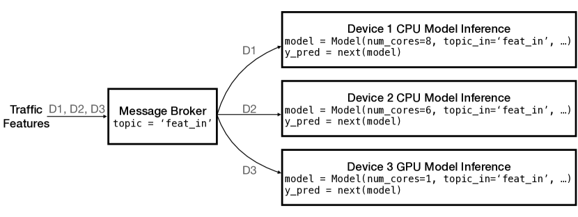
Figure 5. ServeFlow supports parallelism across heterogeneous hardware.

4.3. Model Crafting Pipeline

To support ServeFlow’s fast-slow architecture, an automated training pipeline is integral. This process starts with loading a training set, where the pipeline generates nPrints for each flow, effectively converting network data into a model-friendly format. The key to this stage is the removal of redundant information to optimize feature quality: it eliminates columns with uniform values and those duplicating others. This step ensures the retention of only unique, informative features, enhancing the models’ learning efficiency. It supports a variety of training frameworks (e.g., PyTorch (Paszke et al., 2019), TensorFlow (Abadi et al., 2015), Scikit learn (Pedregosa et al., 2011), LightGBM (Ke et al., 2017b), XGBoost (Chen and Guestrin, 2016), etc.) for users to build highly customized models.

The next phase involves training a pool of models using these refined features from the initial packets (up to N). Each model undergoes an evaluation of its inference speed and performance on a validation set. This comprehensive assessment allows for the selection of models best suited for different roles within ServeFlow- fastest, fast, and slow. For inferences based on a single-packet flow, the fastest model is chosen for its lowest latency, while the fast model is decided through trial and error iterations - which ensures the least flow portion to assign while achieving high F1 scores. The slow model is the one with the best F1-score among all. These selected models, together with their input feature formats (i.e., subscriptions), are transformed into ONNX format (developers, 2021), which enables inter-operability across different frameworks and tools for efficient model optimization and serving. They are later deployed in the fast-slow architecture.

4.4. Implementation

Our system integrates several key technologies to create a robust machine learning solution for network traffic analysis, leveraging the strengths of nPrint (Holland et al., 2021b) with PF_RING (ntop, 2024) for efficient packet capture, EdgeServe (Shaowang and Krishnan, 2023) for low-latency model serving, and a combination of Scikit-learn (Pedregosa et al., 2011), Torch (Paszke et al., 2019), LightGBM (Ke et al., 2017b), and ONNX (developers, 2021) for model training, evaluation, and deployment. This comprehensive setup enables us to handle diverse computational needs effectively.

For packet capture and initial processing, we use nPrint in conjunction with PF_RING C APIs, enhancing our ability to capture network packets quickly in an expressive manner. This forms the foundation of our data preparation phase, ensuring that we have high-quality data for model training and inference. PF_RING_PROMISC enables promiscuous mode on the network interface, allowing it to capture all packets on the network segment it’s attached to, not just those addressed to it. Following the original design of nPrint, we implement using PF_RING APIs to get 1024 bits from IPv4, TCP, and UDP headers in default nPrint. We further enabled dynamic feature subscriptions.

Our machine learning models range from simpler structures like Decision Trees, (at least 15 samples per leaf for enhanced uncertainty characterization), Random Forest to more complex configurations such as CNNs. For gradient boosting models, we employ LightGBM (learning rate 0.03, number of leaves 128, feature fraction 0.9, minimum data in leaf 3) and XGBoost (100 estimators), each carefully tuned with specific parameters to optimize performance. The architecture of our CNN model is designed to process inputs effectively, featuring layers for convolution, pooling, and fully connected operations, alongside dropout for regularization. The model’s structure is tailored to the sequential nature of network packet data, with adjustments made based on the input data’s dimensions. These models are trained using datasets prepared and loaded into our system after ONNX for model conversion, adhering to operator set version 12 and machine learning operator set version 2 for compatibility.

For model serving, EdgeServe plays a pivotal role. As a low-latency streaming system designed for decentralized prediction, it facilitates intra-edge message routing and communication. This capability allows all nodes within the system to produce and consume both data and predictions efficiently, supporting the dynamic integration of multiple data streams for enhanced prediction accuracy. EdgeServe’s integration enables each model to process inputs independently, beginning with the fast model for the first packet of each flow. This model’s predictions are immediately used for decision-making unless deemed unsatisfactory by our flow selection algorithm. In such cases, or when more detailed analysis is required, the slow model takes over, incorporating additional features and subsequent packets. This dual-model approach, supported by a caching mechanism for managing asynchronous data arrival and a FIFO strategy for cache clearing, ensures that our system not only meets the accuracy requirements but also maintains efficiency and responsiveness across various operational scenarios. For deployment using ONNX Runtime, we specify inter- and intra-operation parallelism to be both 1.

5. Evaluation

In this section, we holistically evaluate the performance of ServeFlow across three datasets collected in the real world.

5.1. Evaluation Settings

We detail our tasks, datasets and testbed used for evaluation, consisting of three unique settings.

Service Recognition.

Service recognition plays a vital role in tasks such as resource allocation and Quality of Service (QoS) assurance (Piet et al., 2023; Guthula et al., 2023). In the dataset detailed in Table 6 (in Appendix A), the focus is on categorizing network flows across 4 macro services encompassing 11 distinct classes of applications. This compilation includes a total of 23,487 flows, demonstrating the diversity and complexity of network traffic involved in classifying services for enhanced network management and service delivery.

Device Identification.

Identifying IoT devices is a critical step in mitigating attacks by isolating these devices through communication restrictions from firewalls or gateways (Salman et al., 2022; Aksoy and Gunes, 2019). We leverage the open-source dataset from AMIR (Liu et al., 2023b), which features a diverse collection of 18 in-home devices and encompasses 50,017 unique flows, as documented in Table 7. A notable characteristic of this dataset is the prevalence of short-lived flows, which informs our decision to utilize 3 packets for analysis in the slow model.

QoE Measurement.

QoE measurement on encrypted traffic is an important piece for the management of video streaming applications (Mangla et al., 2018; Mazhar and Shafiq, 2018; Bronzino et al., 2019) or video conferencing apps (VCA) (Sharma et al., 2023; MacMillan et al., 2021). We use the in-lab datasets from (Sharma et al., 2023) for per-second estimates of key VCA QoE metrics such as frame rate. As shown in Table 8, it has a total of 36,928 seconds of data across Meet, Webex, and Teams to make inferences on. The assessment categorizes target frame rates into 11 tiers, incrementing by 3 frames per second up to a threshold beyond 30 fps. This task diverges from the previous two by necessitating continuous inference by ServeFlow, requiring it to monitor flows and update inferences on a second-to-second basis.

Testbed Configuration.

For our experiments, the datasets are split into 50% for training, 10% for validation, and 40% for testing. We develop and test a range of models including Decision Tree, Random Forest, LightGBM, XGBoost, and CNN, across scenarios from handling the first 1 packet to the first 10 packets. These models are later placed at different locations of ServeFlow for evaluations.

To accurately simulate network conditions and maintain the original packet inter-arrival times, we modify the testing set by adjusting time stamps and altering their five-tuple identifiers before merging them into new pcap files. These modified flows range from 200 to 60,000 per second and are encapsulated into 60-second pcap files. These files are then replayed (by using TCPReplay) to a dummy network interface capable of supporting up to 10Gbps, which is monitored by ServeFlow instances through PF_RING APIs. The testbed is running on an AMD EPYC 7302P 16-core 32-thread processor equipped with 64GB RAM, which is a single lab server. Each consumer is an instance subscribing to the incoming data stream. To evaluate system performance, we intentionally restrict the processing to a single consumer if not otherwise specified.

5.2. System Performance

In this section, we evaluate the performance of our proposed system. We compare ServeFlow against two baseline approaches, namely, Best Effort and Queueing-based serving.

• Best Effort. It is applied once the flow features are fully extracted, allowing the model to immediately make a prediction. We achieve the best effort baseline through the use of PF_RING-supported nPrint extraction, directly feeding the features into an ONNX-optimized model for prediction. Both the extraction and prediction processes are executed in C++ within the same thread.

• Queueing. In this approach, extracted flow features are placed into an in-memory queue and processed in a First-In, First-Out sequence. The implementation of queueing mirrors that of ServeFlow but diverges by excluding the fast-slow architecture component.

The baseline approaches are configured to perform model inference using the best N packets of each flow (N identified with the most performant model). ServeFlow is configured to achieve its best possible performance-accuracy tradeoff. We evaluate this tradeoff in the remaining sections of the evaluation. ServeFlow is able to achieve a similar F1 score compared to running all requests to slow model. Following the architecture illustrated in Figure 4, ServeFlow uses a decision tree on the first packet as the fastest model, a LightGBM model on the first packet as the fast model, and another LightGBM model on the ten first packets as the slow model. Further, ServeFlow assigns requests from the fastest to the fast model according to the Uncertainty approach and from the fast to the slow model using the Per-Class Uncertainty approach. In the interest of space, we focus on the service recognition task. We note that we observed similar results for the other tasks (see Appendix B).

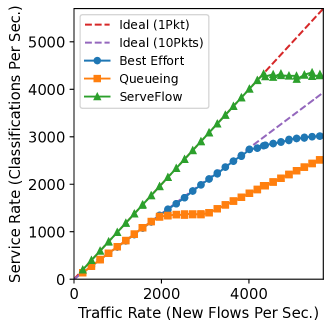
(a)

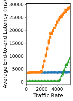
(b)

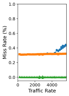
(c)

Figure 6. Performance of different approaches for the service recognition task. We compare ServeFlow against two baselines, Best Effort and Queueing, both considering ten-packet inputs.

Service rate, end-to-end latency, and miss rate.

We define service rate as the number of predicted flows per second; end-to-end latency as the total time spent for a flow between its first packet is produced and a satisfactory prediction is issued, and miss rate as the percentage of flows without a prediction issued by the model. Figure 6 presents (a) the single-consumer service rate, (b) the average end-to-end latency, and (c) flow miss rate for approaches as a function of the network traffic rate, i.e., the number of new flows arriving per second. In Fig. LABEL:fig:trp_comp we also include two lines, i.e., Ideal (1Pkt) and Ideal (10Pkts), to indicate the effective traffic rate when the approaches have to wait for one or ten packets before inference, respectively.

From the figures, we observe that ServeFlow achieves better throughput than the other approaches, keeping up with the traffic rate for a single packet up until around 4.3k flows per second. We also observe that the average latency for ServeFlow is consistently several orders of magnitude smaller than the Best Effort approach before resource saturation. And it achieves 0.0% miss rate because of internal queues, as well as precise-number flow tracking because it does not have to wait for 10 entire packets for a flow.

In contrast, Queueing saturates at around two thousand flows per second while Best Effort keeps the latency consistent due to missing flows. Both of them get a high flow miss rate, because a portion of flows don’t have a length of 10 packets, so no inferences are made for these flows. These results evidence ServeFlow’s capacity to improve the overall performance by serving most of the flows confidently with the faster models, which only require a single packet as input. Figure 7 further illustrates this.

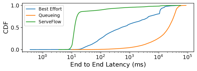
(a)

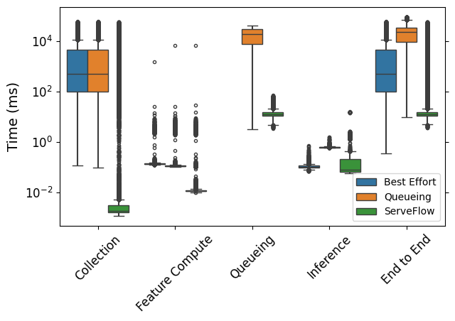
(b)

Figure 7. End-to-end latency analysis for 4k flows per second: (a) The CDF of single-consumer latency demonstrates that ServeFlow can accelerate 76% of flows to millisecond-level service. (b) A breakdown of latency at different stages illustrates the reduction of packet waiting time, showcasing the efficiency of ServeFlow in minimizing overall latency.

Latency breakdown.

For this analysis, we fix the traffic rate at 4k flows per second and plot the CDF for end-to-end latency across inference instances (Fig. LABEL:fig:E2E_CDF). We observe that ServeFlow is capable of serving about 76% of the flows within $16\text{\,}\mathrm{m}\mathrm{s}$. In Fig. LABEL:fig:stage_breakdown, we also analyze the latency breakdown at each serving stage. We note that the collection delay for ServeFlow is about four orders of magnitude faster than the baseline approaches. When compared to the Best Effort approach, the added queueing delay and the marginal increase in the inference delay (due to running multiple models for some flows) are quickly offset by these remarkable savings in the collection stage. All these results together showcase the performance benefits of the proposed fast-slow architecture for network traffic analysis. Next, we evaluate how ServeFlow enables exploring the tradeoff between performance and accuracy for these kind of tasks.

5.3. Flow Assignment Algorithm Performance

The efficiency and accuracy of ServeFlow deeply depend on the performance of assignment approaches under use. We consider four distinct approaches: Oracle, Random, Uncertainty, and Per-class Uncertainty.

• Oracle. It represents an idealized approach that assigns flows based on ground-truth knowledge on classifications being correct or incorrect.

• Random. It denotes a method where decisions on assignment requests are made on a probabilistic basis, with selections being sampled randomly.

• Uncertainty. Algorithm 1 in Section 3.2.

• Per-Class Uncertainty. Algorithm 2 in Section 3.2.

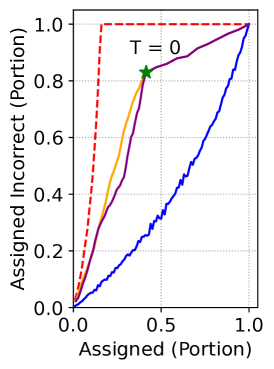
(a)

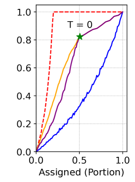
(b)

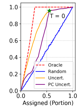
(c)

Figure 8. Assigned portion of requests vs. assigned incorrect portion using different approaches on fastest model (decision tree). T: Uncertainty threshold for the Uncertainty and Per-class Uncertainty approaches.

Assigned vs. assigned incorrect portion.

The goal of assignment approaches is to assign (a) as many incorrectly classified flows as possible, and (b) as few correctly classified ones as possible, from a faster less accurate model to a slower more accurate one. In the ideal case, this maximizes the opportunity for the latter model to correct the mistaken classifications (improving accuracy) while minimizing the overall system end-to-end latency.

We evaluate how well assignment approaches attain this goal. Figure 8 presents the percentage of the incorrect classifications that are assigned as a function of the percentage of overall requests that are assigned by each approach. The curve for Oracle represents the best case scenario for assignments. The percentage of incorrect classifications that are assigned grows quickly reaching 100% when the overall percentage of assigned requests meets the percentage of misclassifications for the fastest inference model (decision tree). Uncertainty and Per-class Uncertainty achieve a good trade-off between the best case scenario (Oracle) and random assignment (note that when the uncertainty threshold arrives 0, the rest of the assignment is random). Both of these approaches assign 82% to 95% of the incorrect classifications when assigning only around 50% of the requests across all the evaluated tasks. For the evaluated model (i.e., decision tree), the Uncertainty approach converges more quickly to the point where the threshold becomes zero, achieving better overall performance.

Assigned portion vs. F1 score.

Given the ability of assignment approaches to discern between correct and incorrect, next we evaluate their impact on the accuracy of the system. We analyze the F1 score of the system after each stage, i.e, after fastest to fast (Fig. LABEL:fig:serv_rec_f2f) and after fast to slow (Fig. LABEL:fig:serv_rec_e2e).

The first insight we draw from these two figures is that: even for Oracle, the best approach to achieve a high F1 score is not to assign everything to a slow model. Because the slow model could be overfitting to some samples, and make correct predictions from faster models faulty. Instead, the most ideal assigned portions are 17% and 7%, respectively.

Uncertainty-based methods show a better balance between Oracle and Random. Essentially, Uncertainty works better for the first stage for decision trees, while Per-Class Uncertainty arrives at a saturated F1 score 6% assignments earlier.

Since ServeFlow configures with the best assignment approach based on different types of models (which will be presented later), it is able to arrive at the best trade-off point earlier than other non-Oracle baselines: around 24% assigned flow to get a 0.962 F1 score on all the flows.

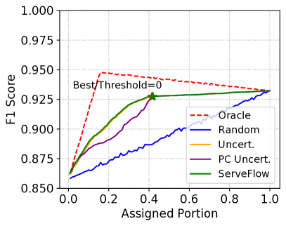
(a)

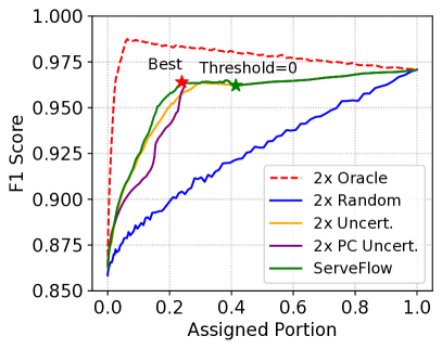
(b)

Figure 9. Assigned portion of requests vs. F1 score at each stage for service recognition task. ServeFlow is best configured to use Uncertainty for the first assignment, and Per-Class Uncertainty for the second.

Fastest	Fast	Slow	Rand.	Uncert.	PC Uncert.
DT			0.514	0.789	0.717
RF	LGBM	LGBM	0.535	0.834	0.789
XGB			0.591	0.674	0.874
CNN			0.468	0.721	0.704

(a) Vary fastest model.

Fastest	Fast	Slow	Rand.	Uncert.	PC Uncert.
	RF		0.664	0.793	0.760
DT	LGBM	LGBM	0.807	0.817	0.838
	XGB		0.459	0.501	0.771
	CNN		0.695	0.789	0.784

(b) Vary fast model.

Table 4. Comparison of Normalized AUC (assigned portion vs. improved F1 score normalized on the Oracle results) across different assignment methods. We vary models in a fastest-fast-slow (DT 1 pkt + LGBM 1 pkt + LGBM 10 pkts) model architecture. Highlighted cells indicate the best performance in each category.

Assignment effectiveness vs. model.

We further investigate that within the ServeFlow architecture examines how different models respond to various assignment strategies. We use the Normalized Area Under Curve (AUC) metric to measure the effectiveness of assignment strategies by comparing the improvement in F1 score relative to the fastest model, normalized against Oracle’s absolute AUC. A higher normalized AUC indicates a better balance between speed and F1 score improvement.

The findings, detailed in Table 4, highlight differences in assignment effectiveness when altering the fastest and fast models in ServeFlow. In scenarios where the fastest model varies (Table 4(a)), Uncertainty-based assignment shows greater benefits for Decision Trees and Random Forest. Conversely, Per-Class Uncertainty significantly improves assignment for XGBoost models, demonstrating a notable advantage (0.874 vs. 0.674 for Uncertainty). When the fast model varies, with Decision Tree as the constant fastest model (Table 4(b)), Uncertainty generally fares better for models other than boosting machines. However, Per-Class Uncertainty is particularly effective when LightGBM is the fast model.

This investigation shows that the variability in confidence distribution across classes—owing to how each model type inherently processes and learns from the data—is the crucial factor. For models like DT, RF, and CNN, where this variability is lower or managed in a uniform way (Wehenkel, 1996), a universal Uncertainty threshold suffices. For boosting machines, where variability is high and class-specific nuances are significant (Ke et al., 2017a), Per-Class Uncertainty thresholds become essential to accurately gauge prediction reliability.

5.4. Microbenchmarks

Service rate scalability.

We evaluated how ServeFlow performance scales as more computational resources are made available to it. We determine the maximum service rate that ServeFlow can achieve as we vary the number of consumers used for model inference and report results in Figure 10. For each evaluated configuration, we also report the improvement over the single-consumer performance. As expected, the throughput grows sublinearly due to the additional communication overhead. Nevertheless, by using only 16 consumers on a single server, ServeFlow is already able to keep up with traffic at a rate of over 48.5k new flows per second (the actual flow rate could be higher, as many flows last more than one second), which is in the same order of magnitude as the traffic rate observed in city backbone links (CAIDA, 2024), and more than 3x service rate than the most recent commodity hardware traffic analysis solution AC-DC (Jiang et al., 2023c).

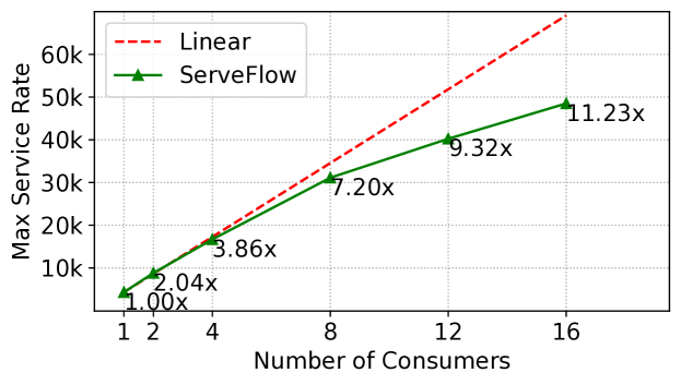
Figure 10. Maximum service rate when we increase the number of consumers. The text along each point is the speed up in service rate compared to a single consumer (4.319k classified flows per second).

ServeFlow performance vs. packet number.

We show the performance changes of ServeFlow when we vary packet number in Table 5. As the number of packets increases from 2 to 10, there’s an improvement in the final F1 score from 0.945 to 0.963. This improvement suggests that analyzing more packets allows for more precise service recognition. However, this accuracy comes at the cost of increased average latency, which escalates from 132.7 ms to 372.2 ms, reflecting the additional waiting and processing time required for larger packet numbers. The median latency remains stable (even 76% because that is the flow portion being served by fast models) across all packet numbers, hovering around 11.2 ms, indicating that the median processing time is largely unaffected by the increase in packet count. Throughput, measured as maximum service rate in thousands of frames per second, shows slight fluctuations but generally remains above 4200 flows per second, peaking at 4319 with 10 packets, which suggests that ServeFlow maintains high efficiency and throughput even as the number of packets for analysis increases. This performance evaluation demonstrates ServeFlow’s capability to balance F1 score, with processing efficiency, as seen in throughput and latency metrics, across different packet analysis depths.

Packet Number	2	4	6	8	10
Final F1 Score	0.945	0.956	0.960	0.962	0.963
Average Latency	132.7	188.5	323.0	358.8	372.2
Median Latency	11.2	11.1	11.3	11.2	11.2
Max Service Rate	4285	4210	4234	4226	4319

Table 5. ServeFlow performance when varying the number of packets on the slow model, for the service recognition task. The unit of latency is ms, and the unit of service rate is classified flows per second.

6. Related Work

Network traffic classification. The study of network traffic and feature selection is crucial in machine learning for networking, evolving with the transition from heuristic-based methods to flow statistics and representation learning. Heuristic methods have declined in reliability due to encryption and internet consolidation (Zheng et al., 2022; Lotfollahi et al., 2020; Boutaba et al., 2018). Current approaches leverage flow statistics like packet numbers and sizes, utilizing tools such as NetFlow and IPFIX (Bernaille et al., 2006; Karagiannis et al., 2005; Claise, 2004, 2008). The advent of advanced machine learning techniques and computational resources has shifted focus towards learning from raw packets for improved accuracy, albeit at the cost of efficiency and interpretability. Deep learning methods, while precise, are criticized for their inefficiency and lack of interpretability compared to traditional machine learning techniques (Lotfollahi et al., 2020; Rimmer et al., 2017; Zheng et al., 2022; Jiang et al., 2023c; Holland et al., 2021b). ServeFlow benefits from representation like nPrint (Holland et al., 2021a) for expressiveness and interpretability, and optimized on the speed to extract them.

Traffic classification serving efficiency. Several systems have been engineered for efficient traffic classification, such as AC-DC (Jiang et al., 2023c), which employs a pool of adaptive models based on constraints and requirements. Others, like NeuroCuts (Liang et al., 2019), focus on optimizing decision trees based on performance criteria. Traffic Refinery specializes in cost-aware model training but lacks automation (Bronzino et al., 2021). Solutions like N3IC (Siracusano et al., 2022), Homunculus (Swamy et al., 2023), and Taurus (Swamy et al., 2022) use specialized hardware to accelerate network traffic classification. pForest (Busse-Grawitz et al., 2022) further explores the trade-off between packet waiting time and classification accuracy by training a sequence of random forest models for different phases of a flow on a programmable switch. The requirement for specialized hardware often implies a lack of complex operations (e.g., floating-point operations), a significant engineering effort (e.g. building ML models in a domain-specific language), and a limited opportunity for parallelism.

A separate vein of research explores low-latency traffic classification. Some methods emphasize model simplification for efficiency (Koksal et al., 2022; Qiu et al., 2022; Tong et al., 2014), while others utilize ensemble or tree-based algorithms (Devprasad et al., 2022; Liu et al., 2019). However, these approaches generally focus on model execution and neglect the optimization of feature space and preprocessing.

Early flow detection methods aim for latency-aware efficiency. For example, early application identification techniques can classify traffic using just a few packets (Bernaille et al., 2006), an idea also incorporated in methods like AC-DC (Jiang et al., 2023c) and the design of ServeFlow.

Low-latency model serving. Various model-serving systems like InferLine, AlpaServe, AdaInf, and MArk similarly strive to reduce the latency of model serving while maintaining model performance (Crankshaw et al., 2020; Li et al., 2023; Shubha and Shen, 2023; Zhang et al., 2019; Crankshaw et al., 2017; Romero et al., 2021). ServeFlow draws upon some of these ideas in its implementation (e.g., abstractions for heterogeneous hardware), but distinguishes itself through its fast-slow architecture optimized for making predictions on partial information, which is especially well-suited for networking applications.

Active learning and sample selection. Recent literature has demonstrated the application of active learning techniques (Settles, 2009) across various domains, including network traffic classification (Shahraki et al., 2022), human activity recognition (Liu et al., 2023b), text classification (Hoi et al., 2006), image classification (Joshi et al., 2012), and cancer diagnosis (Liu, 2004). This approach judiciously selects a subset of data for training, thereby reducing the overall volume of data to be manually labeled. This selective process significantly lowers the human labor involved in labeling, which is a notable benefit given the costly nature of acquiring labeled data. Despite the extensive application of active learning in training tasks, its potential in real-time inference tasks remains largely unexplored. We extend the principles of active learning to real-time inference scenarios: sample selection inherently implies a reduction in both computation and communication workloads, which directly correlates to a lower end-to-end latency. This efficiency, particularly critical in real-time systems, could potentially revolutionize the speed and responsiveness of such systems.

7. Conclusion

This paper presents ServeFlow, a novel fast-slow model architecture tailored for networking ML pipelines. ServeFlow strategically assigns flows to a slower model only when the fastest model’s output is unsatisfactory. Our evaluation shows that ServeFlow is capable of serving the flow rate of city-level network backbones, achieving a 40.5x speedup in median end-to-end latency on a 16-core CPU commodity server. Future research could explore extending the introduced techniques to broader ML pipelines, such as enhancing real-time video analytics or edge computing with a fast-slow model approach. Exploring a cascading system of models that balance system cost and performance offers potential, with ServeFlow’s infrastructure possibly providing a basis for efficient data flow management between models.

Appendix A Datasets

We present the detailed descriptions of the three datasets we have evaluated in Table 6, 7, and 8.

Appendix B Extended evaluations

Service rate, end-to-end latency, and miss rate.

For device identification, figure 11 shows that ServeFlow achieves better service rate (5.2kfps) than others. The uprise of latency is because the two queues get congested at different paces.

Assigned portion vs. F1 score.

Figure 12 and 13 show the effectiveness of assignment algorithms for device identification and QoE measurement task.

Service	Application	# of Flows
Video Conferencing (MacMillan et al., 2021)	Zoom	1312
	Google Meet	1313
	MS Teams	3886
Video Streaming (Bronzino et al., 2019)	Twitch	1150
	Amazon	1509
	YouTube	2702
	Netflix	4104
Social Media	Instagram	873
	Twitter	1260
	Facebook	1477
Smart Home (Liu et al., 2023b)	Other	3901
Total	-	23487

Table 6. Service Recognition Dataset

Device	# of Flows
Samsung Fridge	3770
Nvidia Jetson Nano	3770
Amazon Echo 3rd Gen	3770
Google Home	3770
Raspberry Pi 3	3770
SmartThings Dishwasher	3770
Philips Lightbulb	3770
GE Washer	3770
GE Dryer	3770
Other	3770
LG Nexus 5	3057
Nest Camera	2543
Bose SoundTouch 30	1875
TP-Link Router AC1750	1523
Samsung Galaxy J3	1215
TP-Link Smart Plug HS100	1124
iRobot Vacuum	728
Apple MacBook Pro	252
Total	50017

Table 7. Device Identification Dataset Description.

VCA	Total # of Seconds
Meet	10189
Webex	12331
Teams	14408
Total	36928

Table 8. Video Conferencing Application (VCA) QoE Measurement Dataset Description.

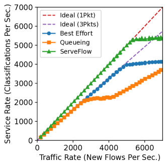
(a)

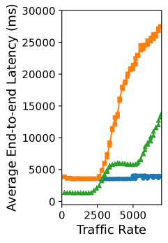
(b)

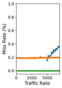
(c)

Figure 11. Performance of different approaches for the device identification task. We compare ServeFlow against two baselines, Best Effort and Queueing, both considering three-packet inputs.

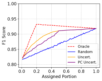
(a)

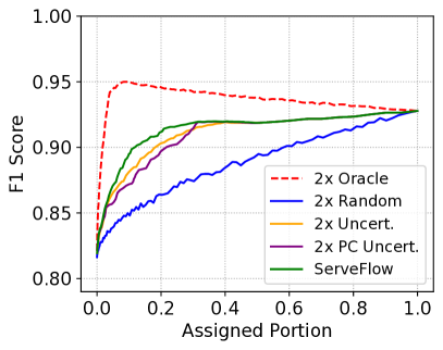
(b)

Figure 12. Assigned portion of requests vs. F1 score at each stage for device identification task.

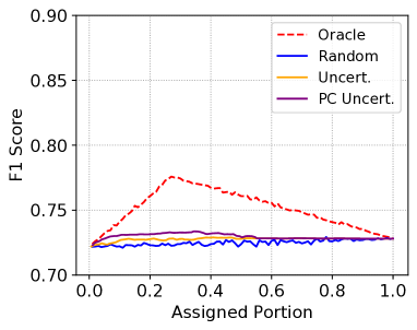
(a)

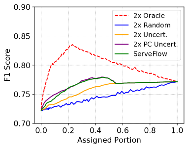
(b)

Figure 13. Assigned portion of requests vs. F1 score at each stage for QoE measurement task.

References

- (1)
- Abadi et al. (2015) Martín Abadi, Ashish Agarwal, Paul Barham, Eugene Brevdo, Zhifeng Chen, Craig Citro, Greg S. Corrado, Andy Davis, Jeffrey Dean, Matthieu Devin, Sanjay Ghemawat, Ian Goodfellow, Andrew Harp, Geoffrey Irving, Michael Isard, Yangqing Jia, Rafal Jozefowicz, Lukasz Kaiser, Manjunath Kudlur, Josh Levenberg, Dandelion Mané, Rajat Monga, Sherry Moore, Derek Murray, Chris Olah, Mike Schuster, Jonathon Shlens, Benoit Steiner, Ilya Sutskever, Kunal Talwar, Paul Tucker, Vincent Vanhoucke, Vijay Vasudevan, Fernanda Viégas, Oriol Vinyals, Pete Warden, Martin Wattenberg, Martin Wicke, Yuan Yu, and Xiaoqiang Zheng. 2015. TensorFlow: Large-Scale Machine Learning on Heterogeneous Systems. (2015). https://www.tensorflow.org/ Software available from tensorflow.org.
- Ahmad et al. (2021) Zeeshan Ahmad, Adnan Shahid Khan, Cheah Wai Shiang, Johari Abdullah, and Farhan Ahmad. 2021. Network intrusion detection system: A systematic study of machine learning and deep learning approaches. Transactions on Emerging Telecommunications Technologies 32, 1 (2021), e4150.
- Aksoy and Gunes (2019) Ahmet Aksoy and Mehmet Hadi Gunes. 2019. Automated iot device identification using network traffic. In ICC 2019-2019 IEEE international conference on communications (ICC). IEEE, 1–7.
- Bernaille et al. (2006) Laurent Bernaille, Renata Teixeira, and Kavé Salamatian. 2006. Early Application Identification. In International Conference on Emerging Networking Experiments and Technologies (CoNEXT).
- Boutaba et al. (2018) Raouf Boutaba, Mohammad A. Salahuddin, Noura Limam, Sara Ayoubi, Nashid Shahriar, Felipe Estrada-Solano, and Oscar M. Caicedo. 2018. A comprehensive survey on machine learning for networking: evolution, applications and research opportunities. In Journal of Internet Services and Applications.
- Bronzino et al. (2021) Francesco Bronzino, Paul Schmitt, Sara Ayoubi, Hyojoon Kim, Renata Teixeira, and Nick Feamster. 2021. Traffic Refinery: Cost-Aware Data Representation for Machine Learning on Network Traffic. In Proceedings of the ACM on Measurement and Analysis of Computing Systems.
- Bronzino et al. (2019) Francesco Bronzino, Paul Schmitt, Sara Ayoubi, Guilherme Martins, Renata Teixeira, and Nick Feamster. 2019. Inferring Streaming Video Quality from Encrypted Traffic: Practical Models and Deployment Experience. In Proceedings of the ACM on Measurement and Analysis of Computing Systems.
- Busse-Grawitz et al. (2022) Coralie Busse-Grawitz, Roland Meier, Alexander Dietmüller, Tobias Bühler, and Laurent Vanbever. 2022. pForest: In-Network Inference with Random Forests. In arXiv:1909.05680v2.
- CAIDA (2024) CAIDA. 2024. CAIDA Backbone Traces. (2024). https://www.caida.org/catalog/datasets/trace_stats/ Accessed: 2024-02-01.
- Chen and Guestrin (2016) Tianqi Chen and Carlos Guestrin. 2016. XGBoost: A Scalable Tree Boosting System. In Proceedings of the 22nd ACM SIGKDD International Conference on Knowledge Discovery and Data Mining (KDD ’16). ACM, New York, NY, USA, 785–794. https://doi.org/10.1145/2939672.2939785
- Claise (2004) Benoit Claise. 2004. Cisco systems netflow services export version 9. Technical Report.
- Claise (2008) Benoit Claise. 2008. Specification of the IP flow information export (IPFIX) protocol for the exchange of IP traffic flow information. Technical Report.
- Crankshaw et al. (2020) Daniel Crankshaw, Gur-Eyal Sela, Xiangxi Mo, Corey Zumar, Ion Stoica, Joseph Gonzalez, and Alexey Tumanov. 2020. InferLine: latency-aware provisioning and scaling for prediction serving pipelines. In Proceedings of the 11th ACM Symposium on Cloud Computing. 477–491.
- Crankshaw et al. (2017) Daniel Crankshaw, Xin Wang, Giulio Zhou, Michael J. Franklin, Joseph E. Gonzalez, and Ion Stoica. 2017. Clipper: A Low-Latency Online Prediction Serving System. In USENIX Symposium on Networked Systems Design and Implementation (NSDI).
- developers (2021) ONNX Runtime developers. 2021. ONNX Runtime. https://onnxruntime.ai/. (2021).
- Devprasad et al. (2022) Kayathri Devi Devprasad, Sukumar Ramanujam, and Suresh Babu Rajendran. 2022. Context adaptive ensemble classification mechanism with multi-criteria decision making for network intrusion detection. Concurrency and Computation: Practice and Experience 34, 21 (2022), e7110.
- Fan et al. (2020) Angela Fan, Pierre Stock, Benjamin Graham, Edouard Grave, Rémi Gribonval, Herve Jegou, and Armand Joulin. 2020. Training with quantization noise for extreme model compression. arXiv preprint arXiv:2004.07320 (2020).
- Fang et al. (2023) Gongfan Fang, Xinyin Ma, Mingli Song, Michael Bi Mi, and Xinchao Wang. 2023. Depgraph: Towards any structural pruning. In Proceedings of the IEEE/CVF Conference on Computer Vision and Pattern Recognition. 16091–16101.
- Ghimire et al. (2022) Deepak Ghimire, Dayoung Kil, and Seong-heum Kim. 2022. A survey on efficient convolutional neural networks and hardware acceleration. Electronics 11, 6 (2022), 945.
- Gou et al. (2021) Jianping Gou, Baosheng Yu, Stephen J Maybank, and Dacheng Tao. 2021. Knowledge distillation: A survey. International Journal of Computer Vision 129 (2021), 1789–1819.
- Guthula et al. (2023) Satyandra Guthula, Navya Battula, Roman Beltiukov, Wenbo Guo, and Arpit Gupta. 2023. netFound: Foundation Model for Network Security. arXiv preprint arXiv:2310.17025 (2023).
- Hoi et al. (2006) Steven C. H. Hoi, Rong Jin, and Michael R. Lyu. 2006. Large-scale text categorization by batch mode active learning. In Proceedings of the 15th International Conference on World Wide Web (WWW ’06). Association for Computing Machinery, New York, NY, USA, 633–642. https://doi.org/10.1145/1135777.1135870
- Holland et al. (2021a) Jordan Holland, Paul Schmitt, Nick Feamster, and Prateek Mittal. 2021a. New Directions in Automated Traffic Analysis. In ACM Conference on Computer and Communications Security (CCS). Seoul, Korea, 1–14. https://www.sigsac.org/ccs/CCS2021/
- Holland et al. (2021b) Jordan Holland, Paul Schmitt, Nick Feamster, and Prateek Mittal. 2021b. New directions in automated traffic analysis. In Proceedings of the 2021 ACM SIGSAC Conference on Computer and Communications Security. 3366–3383.
- Hu and Krishnamachari (2020) Diyi Hu and Bhaskar Krishnamachari. 2020. Fast and accurate streaming CNN inference via communication compression on the edge. In 2020 IEEE/ACM Fifth International Conference on Internet-of-Things Design and Implementation (IoTDI). IEEE, 157–163.
- Hu et al. (2021) Edward J Hu, Yelong Shen, Phillip Wallis, Zeyuan Allen-Zhu, Yuanzhi Li, Shean Wang, Lu Wang, and Weizhu Chen. 2021. Lora: Low-rank adaptation of large language models. arXiv preprint arXiv:2106.09685 (2021).
- Jiang et al. (2023a) Xi Jiang, Shinan Liu, Aaron Gember-Jacobson, Arjun Nitin Bhagoji, Paul Schmitt, Francesco Bronzino, and Nick Feamster. 2023a. NetDiffusion: Network Data Augmentation Through Protocol-Constrained Traffic Generation. arXiv preprint arXiv:2310.08543 (2023).
- Jiang et al. (2023b) Xi Jiang, Shinan Liu, Aaron Gember-Jacobson, Paul Schmitt, Francesco Bronzino, and Nick Feamster. 2023b. Generative, High-Fidelity Network Traces. (2023).
- Jiang et al. (2023c) Xi Jiang, Shinan Liu, Saloua Naama, Francesco Bronzino, Paul Schmitt, and Nick Feamster. 2023c. AC-DC: Adaptive Ensemble Classification for Network Traffic Identification. In arXiv:2302.11718.
- Joshi et al. (2012) Ajay J. Joshi, Fatih Porikli, and Nikolaos P. Papanikolopoulos. 2012. Scalable Active Learning for Multiclass Image Classification. IEEE Trans. Pattern Anal. Mach. Intell. 34, 11 (2012), 2259–2273. https://doi.org/10.1109/TPAMI.2012.21
- Karagiannis et al. (2005) Thomas Karagiannis, Konstantina Papagiannaki, and Michalis Faloutsos. 2005. BLINC: multilevel traffic classification in the dark. In Proceedings of the 2005 conference on Applications, technologies, architectures, and protocols for computer communications. 229–240.
- Ke et al. (2017a) Guolin Ke, Qi Meng, Thomas Finley, Taifeng Wang, Wei Chen, Weidong Ma, Qiwei Ye, and Tie-Yan Liu. 2017a. Lightgbm: A highly efficient gradient boosting decision tree. Advances in neural information processing systems 30 (2017).
- Ke et al. (2017b) Guolin Ke, Qi Meng, Thomas Finley, Taifeng Wang, Wei Chen, Weidong Ma, Qiwei Ye, and Tie-Yan Liu. 2017b. LightGBM: a highly efficient gradient boosting decision tree. In Proceedings of the 31st International Conference on Neural Information Processing Systems (NIPS’17). Curran Associates Inc., Red Hook, NY, USA, 3149–3157.
- Khraisat et al. (2019) Ansam Khraisat, Iqbal Gondal, Peter Vamplew, and Joarder Kamruzzaman. 2019. Survey of intrusion detection systems: techniques, datasets and challenges. Cybersecurity 2, 1 (July 2019), 20. https://doi.org/10.1186/s42400-019-0038-7
- Koksal et al. (2022) Oguz Kaan Koksal, Recep Temelli, Huseyin Ozkan, and Ozgur Gurbuz. 2022. Markov Model Based Traffic Classification with Multiple Features. In 2022 International Balkan Conference on Communications and Networking (BalkanCom). IEEE, 173–177.
- Li et al. (2021) Shuang Li, Jinming Zhang, Wenxuan Ma, Chi Harold Liu, and Wei Li. 2021. Dynamic domain adaptation for efficient inference. In Proceedings of the IEEE/CVF conference on computer vision and pattern recognition. 7832–7841.
- Li et al. (2023) Zhuohan Li, Lianmin Zheng, Yinmin Zhong, Vincent Liu, Ying Sheng, Xin Jin, Yanping Huang, Zhifeng Chen, Hao Zhang, Joseph E Gonzalez, et al. 2023. AlpaServe: Statistical Multiplexing with Model Parallelism for Deep Learning Serving. arXiv preprint arXiv:2302.11665 (2023).
- Liang et al. (2019) Eric Liang, Hang Zhu, Xin Jin, and Ion Stoica. 2019. Neural packet classification. In Proceedings of the ACM Special Interest Group on Data Communication. 256–269.
- Liu and Lang (2019) Hongyu Liu and Bo Lang. 2019. Machine Learning and Deep Learning Methods for Intrusion Detection Systems: A Survey. Applied Sciences 9, 20 (Jan. 2019), 4396. https://doi.org/10.3390/app9204396 Number: 20 Publisher: Multidisciplinary Digital Publishing Institute.
- Liu et al. (2023a) Shinan Liu, Francesco Bronzino, Paul Schmitt, Arjun Nitin Bhagoji, Nick Feamster, Hector Garcia Crespo, Timothy Coyle, and Brian Ward. 2023a. LEAF: Navigating Concept Drift in Cellular Networks. Proceedings of the ACM on Networking 1, CoNEXT2 (2023), 1–24.
- Liu et al. (2023b) Shinan Liu, Tarun Mangla, Ted Shaowang, Jinjin Zhao, John Paparrizos, Sanjay Krishnan, and Nick Feamster. 2023b. AMIR: Active Multimodal Interaction Recognition from Video and Network Traffic in Connected Environments. Proceedings of the ACM on Interactive, Mobile, Wearable and Ubiquitous Technologies 7, 1 (2023). https://doi.org/10.1145/3580818
- Liu (2004) Ying Liu. 2004. Active Learning with Support Vector Machine Applied to Gene Expression Data for Cancer Classification. Journal of Chemical Information and Computer Sciences 44, 6 (2004), 1936–1941. https://doi.org/10.1021/ci049810a arXiv:https://doi.org/10.1021/ci049810a PMID: 15554662.
- Liu et al. (2019) Zhen Liu, Nathalie Japkowicz, Ruoyu Wang, and Deyu Tang. 2019. Adaptive learning on mobile network traffic data. Connection Science 31, 2 (2019), 185–214.
- Liu et al. (2018) Zhuang Liu, Mingjie Sun, Tinghui Zhou, Gao Huang, and Trevor Darrell. 2018. Rethinking the value of network pruning. arXiv preprint arXiv:1810.05270 (2018).
- Lotfollahi et al. (2020) Mohammad Lotfollahi, Mahdi Jafari Siavoshani, Ramin Shirali Hossein Zade, and Mohammdsadegh Saberian. 2020. Deep packet: A novel approach for encrypted traffic classification using deep learning. Soft Computing 24, 3 (2020), 1999–2012.
- MacMillan et al. (2021) Kyle MacMillan, Tarun Mangla, James Saxon, and Nick Feamster. 2021. Measuring the Performance and Network Utilization of Popular Video Conferencing Applications. In ACM SIGCOMM Internet Measurement Conference (IMC). Virtual, 1–14. https://conferences.sigcomm.org/imc/2021/
- Mangla et al. (2018) Tarun Mangla, Emir Halepovic, Mostafa Ammar, and Ellen Zegura. 2018. emimic: Estimating http-based video qoe metrics from encrypted network traffic. In 2018 Network Traffic Measurement and Analysis Conference (TMA). IEEE, 1–8.
- Mazhar and Shafiq (2018) M. Hammad Mazhar and Zubair Shafiq. 2018. Real-time Video Quality of Experience Monitoring for HTTPS and QUIC. In IEEE INFOCOM Conference on Computer Communications.
- Mittal et al. (2023) Meenakshi Mittal, Krishan Kumar, and Sunny Behal. 2023. Deep learning approaches for detecting DDoS attacks: A systematic review. Soft computing 27, 18 (2023), 13039–13075.
- ntop (2024) ntop. 2024. (Feb 2024). https://www.ntop.org/products/packet-capture/pf_ring/
- Olston et al. (2017) Christopher Olston, Fangwei Li, Jeremiah Harmsen, Jordan Soyke, Kiril Gorovoy, Li Lao, Noah Fiedel, Sukriti Ramesh, and Vinu Rajashekhar. 2017. TensorFlow-Serving: Flexible, High-Performance ML Serving. In Workshop on ML Systems at NIPS 2017.
- Paszke et al. (2019) Adam Paszke, Sam Gross, Francisco Massa, Adam Lerer, James Bradbury, Gregory Chanan, Trevor Killeen, Zeming Lin, Natalia Gimelshein, Luca Antiga, et al. 2019. Pytorch: An imperative style, high-performance deep learning library. Advances in neural information processing systems 32 (2019).
- Pedregosa et al. (2011) F. Pedregosa, G. Varoquaux, A. Gramfort, V. Michel, B. Thirion, O. Grisel, M. Blondel, P. Prettenhofer, R. Weiss, V. Dubourg, J. Vanderplas, A. Passos, D. Cournapeau, M. Brucher, M. Perrot, and E. Duchesnay. 2011. Scikit-learn: Machine Learning in Python. Journal of Machine Learning Research 12 (2011), 2825–2830.
- Piet et al. (2023) Julien Piet, Dubem Nwoji, and Vern Paxson. 2023. GGFAST: Automating Generation of Flexible Network Traffic Classifiers. In Proceedings of the ACM SIGCOMM 2023 Conference. 850–866.
- Pulsar (2024) Apache Pulsar. 2024. (Feb 2024). https://pulsar.apache.org/
- Qiu et al. (2022) Kun Qiu, Harry Chang, Ying Wang, Xiahui Yu, Wenjun Zhu, Yingqi Liu, Jianwei Ma, Weigang Li, Xiaobo Liu, and Shuo Dai. 2022. Traffic Analytics Development Kits (TADK): Enable Real-Time AI Inference in Networking Apps. In 2022 Thirteenth International Conference on Ubiquitous and Future Networks (ICUFN). IEEE, 392–398.
- Rezaei et al. (2019) Shahbaz Rezaei, Bryce Kroencke, and Xin Liu. 2019. Large-scale Mobile App Identification Using Deep Learning. In IEEE Access.
- Rimmer et al. (2017) Vera Rimmer, Davy Preuveneers, Marc Juarez, Tom Van Goethem, and Wouter Joosen. 2017. Automated website fingerprinting through deep learning. arXiv preprint arXiv:1708.06376 (2017).
- Romero et al. (2021) Francisco Romero, Qian Li, Neeraja J Yadwadkar, and Christos Kozyrakis. 2021. INFaaS: Automated model-less inference serving. In 2021 USENIX Annual Technical Conference (USENIX ATC 21). 397–411.
- Salman et al. (2022) Ola Salman, Imad H Elhajj, Ali Chehab, and Ayman Kayssi. 2022. A machine learning based framework for IoT device identification and abnormal traffic detection. Transactions on Emerging Telecommunications Technologies 33, 3 (2022), e3743.
- Settles (2009) Burr Settles. 2009. Active Learning Literature Survey. Computer Sciences Technical Report 1648. University of Wisconsin–Madison.
- Shahraki et al. (2022) Amin Shahraki, Mahmoud Abbasi, Amir Taherkordi, and Anca Delia Jurcut. 2022. Active Learning for Network Traffic Classification: A Technical Study. IEEE Trans. Cogn. Commun. Netw. 8, 1 (2022), 422–439. https://doi.org/10.1109/TCCN.2021.3119062
- Shaowang and Krishnan (2023) Ted Shaowang and Sanjay Krishnan. 2023. EdgeServe: An Execution Layer for Decentralized Prediction. arXiv preprint arXiv:2303.08028 (2023).
- Shapira and Shavitt (2021) Tal Shapira and Yuval Shavitt. 2021. FlowPic: A Generic Representation for Encrypted Traffic Classification and Applications Identification. In IEEE Transactions on Network and Service Management.
- Sharma et al. (2023) Taveesh Sharma, Tarun Mangla, Arpit Gupta, Junchen Jiang, and Nick Feamster. 2023. Estimating WebRTC Video QoE Metrics Without Using Application Headers. In ACM SIGCOMM Internet Measurement Conference (IMC). Montreal, Canada, 1–12.
- Shubha and Shen (2023) Sudipta Saha Shubha and Haiying Shen. 2023. AdaInf: Data Drift Adaptive Scheduling for Accurate and SLO-guaranteed Multiple-Model Inference Serving at Edge Servers. In Proceedings of the ACM SIGCOMM 2023 Conference. 473–485.
- Siracusano et al. (2022) Giuseppe Siracusano, Salvator Galea, Davide Sanvito, Mohammad Malekzadeh, Gianni Antichi, Paolo Costa, Hamed Haddadi, and Roberto Bifulco. 2022. Re-architecting Traffic Analysis with Neural Network Interface Cards. In USENIX Symposium on Networked Systems Design and Implementation (NSDI).
- Sivanathan et al. (2019) Arunan Sivanathan, Hassan Habibi Gharakheili, Franco Loi, Adam Radford, Chamith Wijenayake, Arun Vishwanath, and Vijay Sivaraman. 2019. Classifying IoT Devices in Smart Environments Using Network Traffic Characteristics. In IEEE Transactions on Mobile Computing.
- Staessens et al. (2011) Dimitri Staessens, Sachin Sharma, Didier Colle, Mario Pickavet, and Piet Demeester. 2011. Software defined networking: Meeting carrier grade requirements. In 2011 18th IEEE workshop on local & metropolitan area networks (LANMAN). IEEE, 1–6.
- Swamy et al. (2022) Tushar Swamy, Alexander Rucker, Muhammad Shahbaz, Ishan Gaur, and Kunle Olukotun. 2022. Taurus: A Data Plane Architecture for Per-Packet ML. In ACM International Conference on Architectural Support for Programming Languages and Operating Systems (ASPLOS).
- Swamy et al. (2023) Tushar Swamy, Annus Zulfiqar, Luigi Nardi, Muhammad Shahbaz, and Kunle Olukotun. 2023. Homunculus: Auto-Generating Efficient Data-Plane ML Pipelines for Datacenter Networks. In ACM International Conference on Architectural Support for Programming Languages and Operating Systems (ASPLOS).
- Tong et al. (2014) Da Tong, Yun R Qu, and Viktor K Prasanna. 2014. High-throughput traffic classification on multi-core processors. In 2014 IEEE 15th International Conference on High Performance Switching and Routing (HPSR). IEEE, 138–145.
- Wang and Yoon (2021) Lin Wang and Kuk-Jin Yoon. 2021. Knowledge distillation and student-teacher learning for visual intelligence: A review and new outlooks. IEEE transactions on pattern analysis and machine intelligence 44, 6 (2021), 3048–3068.
- Wehenkel (1996) Louis Wehenkel. 1996. On uncertainty measures used for decision tree induction. In Ipmu-96, information processing and management of uncertainty in knowledge-based systems.
- Yang et al. ([n. d.]) Kun Yang, Samory Kpotufe, and Nick Feamster. [n. d.]. An Efficient One-Class SVM for Novelty Detection in IoT. ([n. d.]).
- Yang et al. (2020) Yibo Yang, Robert Bamler, and Stephan Mandt. 2020. Improving inference for neural image compression. Advances in Neural Information Processing Systems 33 (2020), 573–584.
- Zhang et al. (2019) Chengliang Zhang, Minchen Yu, Wei Wang, and Feng Yan. 2019. MArk: Exploiting Cloud Services for Cost-Effective,SLO-Aware Machine Learning Inference Serving. In 2019 USENIX Annual Technical Conference (USENIX ATC 19). 1049–1062.
- Zheng et al. (2022) Weiping Zheng, Jianhao Zhong, Qizhi Zhang, and Gansen Zhao. 2022. MTT: an efficient model for encrypted network traffic classification using multi-task transformer. Applied Intelligence (2022), 1–16.