Pard: Permutation-Invariant Autoregressive Diffusion for Graph Generation

Abstract

Graph generation has been dominated by autoregressive models due to their simplicity and effectiveness, despite their sensitivity to ordering. Yet diffusion models have garnered increasing attention, as they offer comparable performance while being permutation-invariant. Current graph diffusion models generate graphs in a one-shot fashion, but they require extra features and thousands of denoising steps to achieve optimal performance. We introduce Pard, a Permutation-invariant AutoRegressive Diffusion model that integrates diffusion models with autoregressive methods. Pard harnesses the effectiveness and efficiency of the autoregressive model while maintaining permutation invariance without ordering sensitivity. Specifically, we show that contrary to sets, elements in a graph are not entirely unordered and there is a unique partial order for nodes and edges. With this partial order, Pard generates a graph in a block-by-block, autoregressive fashion, where each block’s probability is conditionally modeled by a shared diffusion model with an equivariant network. To ensure efficiency while being expressive, we further propose a higher-order graph transformer, which integrates transformer with PPGN (Maron et al., 2019). Like GPT, we extend the higher-order graph transformer to support parallel training of all blocks. Without any extra features, Pard achieves state-of-the-art performance on molecular and non-molecular datasets, and scales to large datasets like MOSES containing 1.9M molecules. Pard is open-sourced at https://github.com/LingxiaoShawn/Pard.

1 Introduction

Graphs provide a powerful abstraction for representing relational information in many domains, including social networks, biological and molecular structures, recommender systems, and networks of various infrastructures such as computers, roads, etc. Accordingly, generative models of graphs that learn the underlying graph distribution from data find applications in network science (Bonifati et al., 2020), drug discovery (Li et al., 2018b; Tong et al., 2021), protein design (Anand & Huang, 2018; Trinquier et al., 2021), and various use-cases for Internet of Things (De et al., 2022). Also, they serve as a prerequisite for building a generative foundation model (Bommasani et al., 2021) for graphs.

Despite significant progress in generative models for images and language, graph generation is uniquely challenged by its inherent combinatorial nature. Specifically: 1) Graphs are naturally high-dimensional and discrete with varying sizes, contrasting with the continuous space and fixed-size advancements that cannot be directly applied here; 2) Being permutation-invariant objects, graphs require modeling an exchangeable probability distribution, where permutations of nodes and edges do not alter the graph’s probability; 3) The rich substructures in graphs necessitate an expressive model capable of capturing higher-order motifs and interactions. Several graph generative models have been proposed to address (part of) these challenges, based on various techniques like autoregression (You et al., 2018; Liao et al., 2019), VAEs (Simonovsky & Komodakis, 2018), GANs (De Cao & Kipf, 2018), flow-based methods (Shi* et al., 2020), and denoising diffusion (Niu et al., 2020; Vignac et al., 2023). Among these, autoregressive models and diffusion models stand out with superior performance, thus significant popularity. However, current autoregressive models, while efficient, are sensitive to order with non-exchangeable probabilities; whereas diffusion models, though promising, are less efficient, requiring thousands of denoising steps and extra features to achieve high generation quality.

In this paper, we introduce Pard (leopard in Ancient Greek), the first Permutation-invariant AutoRegressive Diffusion model that combines the efficiency of autoregressive methods and the quality of diffusion models together, while retaining the property of exchangeable probability. Instead of generating an entire graph directly, we explore the direction of generating through block-wise graph enlargement. Graph enlargement offers a fine-grained control over graph generation, which can be particularly advantageous for real-world applications that require local revisions to generate graphs. Moreover, it essentially decomposes the joint distribution of the graph into a series of simpler conditional distributions, thereby leveraging the data efficiency characteristic of autoregressive modeling. We also argue that graphs, unlike sets, inherently exhibit a unique partial order among nodes, naturally facilitating the decomposition of the joint distribution. Thanks to this unique partial order, Pard’s block-wise sequence is permutation-equivariant.

To model the conditional distribution of nodes and edges in a block, we first show that the corresponding graph transformation cannot be solved directly with any equivariant network no matter how powerful it is. However, through a diffusion process that injects noise, a permutation equivariant network can progressively denoise to realize targeted graph transformations. This approach is inspired by the annealing process where energy is initially heightened before achieving a stable state, akin to the process of tempering iron. Our analytical findings serve as the foundation for the design of our proposed Pard that combines autoregressive approach with local block-wise discrete denoising diffusion. Using a diffusion model with equivariant networks ensures that each block’s conditional distribution is exchangeable. Coupled with the permutation-invariant sequence of blocks, this renders the entire process permutation invariant and the joint distribution exchangeable.

Within Pard, we further propose several architectural improvements. First, to achieve 2-FWL expressivity with improved memory efficiency, we propose a higher-order graph transformer that integrates the transformer framework with PPGN (Maron et al., 2019), while utilizing a significantly reduced representation size for edges. Second, to ensure training efficiency without substantial overhead compared to the original diffusion model, we design a GPT-like causal mechanism to support parallel training of all blocks with shared representations. These extensions are generalizable and can lay the groundwork for a higher-order GPT.

Pard achieves new SOTA performance on many molecular and non-molecular datasets without any extra features, significantly outperforming DiGress (Vignac et al., 2023). Thanks to efficient architecture and parallel training, Pard scales to large datasets like MOSES (Polykovskiy et al., 2020) with 1.9M graphs. Finally, not only Pard can serve as a generative foundation model for graphs in the future, its autoregressive parallel mechanism can further be combined with language models for language-graph generative pretraining, planting seeds for high-potential future work.

2 Related Work

Autoregressive (AR) Models for Graph Generation. AR models create graphs step-by-step, adding nodes and edges sequentially. This method acknowledges graphs’ discrete nature but faces a key challenge as there is no inherent order in graph generation. To address this, various strategies have been proposed to simplify orderings and approximate the marginalization over permutations; i.e. $p(G)=\sum_{\pi\in\mathcal{P}(G)}p(G,\pi)$. Li et al. (2018a) propose using random or deterministic empirical orderings. GraphRNN (You et al., 2018) aligns permutations with breadth-first-search (BFS) ordering, with a many-to-one mapping. GRAN (Liao et al., 2019) offers marginalization over a family of canonical node orderings, including node degree descending, DFS/BFS tree rooted at the largest degree node, and k-core ordering. GraphGEN (Goyal et al., 2020a) uses a single canonical node ordering, but does not guarantee the same canonical ordering during generation. Chen et al. (2021) avoid defining ad-hoc orderings by modeling the conditional probability of orderings, $p(\pi|G)$, with a trainable AR model, estimating marginalized probabilities during training to enhance both the generative model and the ordering probability model.

Diffusion Models for Graph Generation. EDP-GNN (Niu et al., 2020) is the first work that adapts score matching (Song & Ermon, 2019) to graph generation, by viewing graphs as matrices with continuous values. GDSS (Jo et al., 2022) generalizes EDP-GNN by adapting SDE-based diffusion (Song et al., 2021) and considers node and edge features. Yan et al. (2023) argues that learning exchangeable probability with equivariant networks is hard, hence proposes permutation-sensitive SwinGNN with continuous-state score matching. Previous works apply continuous-state diffusion to graph generation, ignoring the natural discreteness of graphs. DiGress (Vignac et al., 2023) is the first to apply discrete-state diffusion (Austin et al., 2021; Hoogeboom et al., 2021) to graph generation and achieves significant improvement. However, DiGress relies on many additional structural and domain-specific features. GraphArm (Kong et al., 2023) applies Autoregressive Diffusion Model (ADM) (Hoogeboom et al., 2022a) to graph generation, where exactly one node and its adjacent edges decay to the absorbing states at each forward step based on a random node order. Similar to AR models, GraphArm is permutation sensitive.

We remark that although both are termed “autoregressive diffusion”, it is important to distinguish that Pard is not equivalent to ADM. The term “autoregressive diffusion” in our context refers to the integration of autoregressive methods with diffusion models. In contrast, ADM represents a specific type of discrete denoising diffusion where exactly one dimension decays to an absorbing state at a time in the forward diffusion process. See Fan et al. (2023) for a comprehensive survey of recent diffusion models on graphs.

3 Autoregressive Denoising Diffusion

We first introduce setting and notations. We focus on graphs with categorical features. Let $G=({\mathcal{V}},{\mathcal{E}})$ be a labeled graph with maximum $K_{v}$ and $K_{e}$ distinct node and edge labels respectively. Let ${\bm{v}}^{i}\in\{0,1\}^{K_{v}},\forall i\in|{\mathcal{V}}|$ be the one-hot encoding of node $i$’s label. Let ${\bm{e}}^{i,j}\in\{0,1\}^{K_{e}},\forall i,j\in|{\mathcal{V}}|$ be the one-hot encoding of the label for the edge between node $i$ and $j$. We also represent “absence of edge” as a type of edge label, hence $|{\mathcal{E}}|=|{\mathcal{V}}|\times|{\mathcal{V}}|$. Let ${\bm{V}}\in\{0,1\}^{|{\mathcal{V}}|\times K_{v}}$ and ${\bm{E}}\in\{0,1\}^{|{\mathcal{V}}|\times|{\mathcal{V}}|\times K_{e}}$ be the collection of one-hot encodings of all nodes and edges. To describe probability, let ${\mathbf{x}}$ be a random variable with its sampled value ${\bm{x}}$. In diffusion process, noises are injected from $t$$=$$0$ to $t$$=$$T$ with $T$ being the maximum time step. Let ${\mathbf{x}}_{0}\sim p_{\text{data}}({\mathbf{x}}_{0})$ be the random variable of observed data with underlying distribution $p_{\text{data}}({\mathbf{x}}_{0})$, ${\mathbf{x}}_{t}\sim q({{\mathbf{x}}_{t}})$ be the random variable at time $t$, and let ${\mathbf{x}}_{t|s}\sim q({\mathbf{x}}_{t}|{\mathbf{x}}_{s})$ be the conditional random variable. Also, we interchangeably use $q({\mathbf{x}}_{t}|{\mathbf{x}}_{s})$, $q({\mathbf{x}}_{t}$$=$${\bm{x}}_{t}|{\mathbf{x}}_{s}$$=$${\bm{x}}_{s})$, and $q_{t|s}({\bm{x}}_{t}|{\bm{x}}_{s})$ when there is no ambiguity. We model the forward diffusion process independently for each node and edge of the graph, while the backward denoising process is modeled jointly for all nodes and edges. All vectors are column-wise vectors. Let $\langle\cdot,\cdot\rangle$ denote inner product.

3.1 Discrete Denoising Diffusion on Graphs

Denoising Diffusion is first developed by Sohl-Dickstein et al. (2015) and later improved by Ho et al. (2020). It is further generalized to discrete-state case by Hoogeboom et al. (2021); Austin et al. (2021). Taking a graph ${\textnormal{G}}_{0}$ as example, diffusion model defines a forward diffusion process to gradually inject noise to all nodes and edges independently until all reach a non-informative state ${\textnormal{G}}_{T}$. Then, a denoising network is trained to reconstruct ${\textnormal{G}}_{0}$ from the noisy sample ${\textnormal{G}}_{t}$ at each time step, by optimizing a Variational Lower Bound (VLB) for $\log p_{\theta}({\textnormal{G}}_{0})$. Specifically, the forward process is defined as a Markov chain with $q({\textnormal{G}}_{t}|{\textnormal{G}}_{t-1}),\forall t\in[1,T]$, and the backward denoising process is parameterized with another Markov chain $p_{\theta}({\textnormal{G}}_{t-1}|{\textnormal{G}}_{t}),\forall t\in[1,T]$. Note that while the forward process is independently applied to all elements, the backward process is coupled together with conditional independence assumption. Formally,

$$q({\textnormal{G}}_{t}|{\textnormal{G}}_{t-1}) =\prod_{i}^{|{\mathcal{V}}|}q({\mathbf{v}}^{i}_{t}|{\mathbf{v}}^{i}_{t-1})\prod_{i,j}^{|{\mathcal{V}}|}q({\mathbf{e}}^{i,j}_{t}|{\mathbf{e}}^{i,j}_{t-1})$$ (1)

$$p_{\theta}({\textnormal{G}}_{t-1}|{\textnormal{G}}_{t}) =\prod_{i}^{|{\mathcal{V}}|}p_{\theta}({\mathbf{v}}^{i}_{t-1}|{\textnormal{G}}_{t})\prod_{i,j}^{|{\mathcal{V}}|}p_{\theta}({\mathbf{e}}^{i,j}_{t-1}|{\textnormal{G}}_{t})\;.$$ (2)

The VLB lower bound can be written (see Apdx.§A.1) as

where the second term is $\approx 0$, since $p_{\theta}({\textnormal{G}}_{T})\approx q({\textnormal{G}}_{T}|{\textnormal{G}}_{0})$ is designed as a fixed noise distribution that is easy to sample from. To compute Eq. (3), we need to formalize the distributions ($i$) $q({\textnormal{G}}_{t}|{\textnormal{G}}_{0})$ and ($ii$) $q({\textnormal{G}}_{t-1}|{\textnormal{G}}_{t},{\textnormal{G}}_{0})$, as well as ($iii$) the parameterization of $p_{\theta}({\textnormal{G}}_{t-1}|{\textnormal{G}}_{t})$.

DiGress (Vignac et al., 2023) applies D3PM’s (Austin et al., 2021) to define these three terms. Since all elements in the forward process are independent as shown in Eq. (1), one can verify that the two terms $q({\textnormal{G}}_{t}|{\textnormal{G}}_{0})$ and $q({\textnormal{G}}_{t-1}|{\textnormal{G}}_{t},{\textnormal{G}}_{0})$ are in the form of a product of independent distributions on each element. For simplicity, we introduce the formulation for a single element ${\mathbf{x}}$, with ${\mathbf{x}}$ being ${\mathbf{v}}^{i}$ or ${\mathbf{e}}^{i,j}$. We assume each discrete random variable ${\mathbf{x}}_{t}$ has a categorical distribution, i.e. ${\mathbf{x}}_{t}\sim\text{Cat}({\mathbf{x}}_{t};{\bm{p}})$ with ${\bm{p}}\in[0,1]^{K}$ and $\bm{1}^{\top}{\bm{p}}=1$ . One can verify that $p({\mathbf{x}}_{t}={\bm{x}}_{t})={\bm{x}}_{t}^{\top}{\bm{p}}$, or simply $p({\mathbf{x}}_{t})={\bm{x}}_{t}^{\top}{\bm{p}}$. As shown in Hoogeboom et al. (2021); Austin et al. (2021), the forward process with discrete variables $q({\mathbf{x}}_{t}|{\mathbf{x}}_{t-1})$ can be represented as a transition matrix $Q_{t}\in[0,1]^{K\times K}$ such that $[Q_{t}]_{ij}=q({\mathbf{x}}_{t}={\bm{e}}_{j}|{\mathbf{x}}_{t-1}={\bm{e}}_{i})$. Then, we can write the distribution explicitly as

$$q({\mathbf{x}}_{t}|{\mathbf{x}}_{t-1})=\text{Cat}({\mathbf{x}}_{t};Q^{\top}_{t}{\bm{x}}_{t-1})\;.$$ (4)

Given transition matrices $Q_{1},...,Q_{T}$, we can get

$$(i)\ q({\mathbf{x}}_{t}|{\mathbf{x}}_{0})=\text{Cat}({\mathbf{x}}_{t};\overline{Q}_{t}^{\top}{\bm{x}}_{0}),\text{with }\overline{Q}_{t}=Q_{1}...Q_{t}\;,$$ (5)

and the $(t$$-$$1)$-step posterior distribution as

See Apdx.§A.2 for the derivation. We have the option to specify node- or edge-specific quantities, $Q_{t}^{v,i}$ and $Q_{t}^{e,{i,j}}$, respectively, or allow all nodes and edges to share a common $Q_{t}^{v}$ and $Q_{t}^{e}$. Leveraging Eq. (5) and Eq. (6), we can precisely determine $q({\mathbf{v}}^{i}_{t}|{\mathbf{v}}^{i}_{0})$ and $q({\mathbf{v}}^{i}_{t-1}|{\mathbf{v}}^{i}_{t},{\mathbf{v}}^{i}_{0})$ for every node, and a similar approach can be applied for the edges. To ensure simplicity and a non-informative $q({\textnormal{G}}_{T}|{\textnormal{G}}_{0})$ (see Apdx.§A.3), we choose

$$Q_{t}=\alpha_{t}I+(1-\alpha_{t})\bm{1}{\bm{m}}^{\top}$$ (7)

for all nodes and edges, where $\alpha_{t}\in[0,1]$, and ${\bm{m}}$ is the probability of a uniform distribution ($\bm{1}/K_{v}$ for nodes and $\bm{1}/K_{e}$ for edges). Note that DiGress (Vignac et al., 2023) chooses ${\bm{m}}$ as the marginal distribution of nodes and edges.

As $p({\mathbf{x}}_{t-1}|{\mathbf{x}}_{t})=\sum_{{\mathbf{x}}_{0}}q({\mathbf{x}}_{t-1}|{\mathbf{x}}_{t},{\mathbf{x}}_{0})p({\mathbf{x}}_{0}|{\mathbf{x}}_{t})$ , the parameterization of $p_{\theta}({\textnormal{G}}_{t-1}|{\textnormal{G}}_{t})$ can use the relationship, with

$$(iii)\quad p_{\theta}({\mathbf{x}}_{t-1}|{\textnormal{G}}_{t})=\sum_{{\mathbf{x}}_{0}}q({\mathbf{x}}_{t-1}|{\mathbf{x}}_{t},{\mathbf{x}}_{0})p_{\theta}({\mathbf{x}}_{0}|{\textnormal{G}}_{t})$$ (8)

where ${\mathbf{x}}$ can be any ${\mathbf{v}}^{i}$ or ${\mathbf{e}}^{i,j}$. With Eq. (8), we can parameterize $p_{\theta}({\mathbf{x}}_{0}|{\textnormal{G}})$ directly with a neural network, and compute the negative VLB loss in Eq. (3) exactly, using Eq.s (5), (6) and (8). In addition, the cross entropy loss between $q({\mathbf{x}}_{t}|{\mathbf{x}}_{0})$ and $p_{\theta}({\mathbf{x}}_{0}|{\textnormal{G}}_{t})$ that quantifies reconstruction quality is often employed as an auxiliary loss as

In fact, DiGress solely uses $\mathcal{L}_{t}^{CE}(\theta)$ to train their diffusion model. In this paper, we adapt a hybrid loss (Austin et al., 2021), i.e. $\mathcal{L}_{t}(\theta)+\lambda\mathcal{L}_{t}^{CE}(\theta)$ with $\lambda=0.1$, as we found it to help reduce overfitting. To generate a graph from $p_{\theta}({\textnormal{G}}_{0})$, a pure noise graph is first sampled from $p_{\theta}({\textnormal{G}}_{T})$ and gradually denoised using the learned $p_{\theta}({\textnormal{G}}_{t-1}|{\textnormal{G}}_{t})$ from step $T$ to 0.

A significant advantage of diffusion models is their ability to achieve exchangeable probability in combination with permutation equivariant networks under certain conditions (Xu et al., 2022). DiGress is the first work that applies discrete denoising diffusion to graph generation, and achieves significant improvement over previous continuous-state based diffusion. However, given the inherently high-dimensional nature of graphs and their complex internal dependencies, modeling the joint distribution of all nodes and edges directly presents significant challenges. DiGress requires thousands of denoising steps to accurately capture the original dependencies. Moreover, DiGress relies on many supplementary features, such as cycle counts and eigenvectors, to effectively break symmetries among structural equivalences to achieve high performance.

3.2 Autoregressive Graph Generation

Order is important for AR models. Unlike diffusion models that aim to capture the joint distribution directly, AR models decompose the joint probability into a product of simpler conditional probabilities based on an order. This makes AR models inherently suitable for ordinal data, where a natural order exists, such as in natural languages and images.

Order Sensitivity. Early works of graph generation contain many AR models like GraphRNN (You et al., 2018) and GRAN (Liao et al., 2019) based on non-deterministic heuristic node orders like BFS/DFS and k-core ordering. Despite being permutation sensitive, AR models achieve SOTA performance on small simulated structures like grid and lobster graphs. However, permutation invariance is necessary for estimating an accurate likelihood probability of a graph, and can benefit large-size datasets for better generalization.

Let $\pi$ denote an ordering of nodes. To make AR order-insensitive, there are two directions: (1) Modeling the joint probability $p({\textnormal{G}},\pi)$ and then marginalizing $\pi$, (2) Finding a unique canonical order $\pi^{*}(G)$ for any graph $G$ such that $p(\pi|{\textnormal{G}})$ = 1 if $\pi=\pi^{*}(G)$ and 0 otherwise. In direction (1), directly integrating out $\pi$ is prohibitive as the number of permutations is factorial in the graph size. Several studies (Li et al., 2018a; Chen et al., 2021; Liao et al., 2019) have investigated the use of subsets of either random or canonical orderings. This approach aims to simplify the process, but it results in approximate integrals with indeterminate errors. Moreover, it escalates computational expense due to the need for data augmentation involving these subsets of orderings. In direction (2), identifying a universal canonical order for all graphs is referred to as graph canonicalization. This task is recognized to be at least as challenging as the Graph Isomorphism problem, which is classified as NP-intermediate. Goyal et al. (2020b) explores using minimum DFS code to construct canonical labels for a specific dataset with non-polynomial time complexity. However, the canonicalization is specific to each training dataset with the randomness derived from DFS. This results in the canonical order being $\pi(G|\text{TrainSet})$ instead of $\pi(G)$, which exhibits the generalization issue.

The Existence of Partial Order. While finding a unique order for all nodes of a graph is NP-intermediate, we argue that finding a unique partial order, where certain nodes and edges are with the same rank, is achievable. For example, a trivial partial order is simply all nodes and edges having the same rank. Nevertheless, a graph is not the same as a set (a set is just a graph with empty ${\mathcal{E}}$), where all elements are essentially unordered with equivalent rank. That is because a non-empty graph contains edges between nodes, and these edges give different structural properties to nodes. Notice that some nodes or edges have the same structural property as they are structurally equivalent. We can view each structural property as a color, and rank all unique colors within the graph to define the partial order over nodes, which we call a structural partial order. The structural partial order defines a sequence of blocks such that all nodes within a block have the same rank (ı.e. color).

Let $\phi:{\mathcal{V}}\rightarrow[1,...,|{\mathcal{S}}|]$ be the function that assigns rank to nodes based on their structural properties. When ${\mathcal{S}}\subseteq{\mathcal{V}}$, we use $G[{\mathcal{S}}]$ to denote the induced subgraph on the subset ${\mathcal{S}}$. There are many ways to assign rank to structural colors, however we would like the resulting partial order to satisfy certain constraints. Most importantly, we want

$$\forall r\in[1,...,|{\mathcal{S}}|],\ G[\phi({\mathcal{V}})\leq r]\text{ is a connected graph.}$$ (9)

The connectivity requirement is to ensure a more accurate representation of real-world graph generation processes, where most real-world dynamic graphs are enlarged with newcoming nodes being connected at any time. Then, one can sequentially remove all nodes with the lowest degree to maintain this connectivity and establish a partial order. However, as degree only reflects information of the first-hop neighbor structure, many nodes share the same degree, leading to only a few distinct blocks, not significantly different from a trivial, single-block approach.

To ensure connectivity while reducing rank collision, we consider larger hops to define a weighted degree. Consider a maximum of $K_{h}$ hops. For any node ${\bm{v}}\in{\mathcal{V}}$, the number of neighbors at each hop of ${\bm{v}}$ can be easily obtained as $[d_{1}({\bm{v}}),...,d_{K_{h}}({\bm{v}})]$. We then define the weighted degree as

$$w_{K_{h}}({\bm{v}})=\sum_{k=1}^{K_{h}}d_{k}({\bm{v}})\times|{\mathcal{V}}|^{K_{h}-k}$$ (10)

Eq. (10) is fast to compute, and ensures that 1) nodes have the same rank if and only if they have the same number of neighbors up to $K_{h}$ hops; and 2) lower-hop degrees are weighted higher such that nodes with smaller lower-hop degree have smaller $w_{K_{h}}$. With $w_{K_{h}}$ defined, we give the structural partial order in Algo. 1. It is important to note that for any $G$, its structural partial order is unique, deterministic, and permutation equivariant. Formally, let ${\bm{P}}$ be any permutation operator, then

$$\phi({\bm{P}}\star G)={\bm{P}}\star\phi(G)$$ (11)

Algorithm 1 Structural Partial Order $\phi$

1:  Input: Graph $G$, maximum hops $K_{h}$.

2:  Init: $G_{0}=G$, $i=0$, $\phi$ with $\phi({\bm{v}})=0\ \forall{\bm{v}}.$

3:  while $G_{i}$ is not $\emptyset$ do

4:     Compute $w_{K_{h}}({\bm{v}}),\forall{\bm{v}}\in{\mathcal{V}}(G_{i}),$ using Eq. (10).

5:     Find all nodes $\mathcal{L}$ with $w_{K_{h}}=\min_{{\bm{v}}\in{\mathcal{V}}(G)}w_{K_{h}}({\bm{v}})$.

6:     Let $\phi({\bm{v}})=i\ \forall{\bm{v}}\in\mathcal{L}$.

7:     $G_{i+1}\leftarrow G_{i}[{\mathcal{V}}(G)\setminus\mathcal{L}]$; $i\leftarrow i+1$.

8:  end while

9:  Output: $\phi\leftarrow i-\phi$

Autoregressive Blockwise Generation. The structural partial order $\phi$ of $G$ in Algo. 1 with output in range $[1,K_{B}]$ divides the nodes ${\mathcal{V}}(G)$ into $K_{B}$ blocks $[{\mathcal{B}}_{1},...,{\mathcal{B}}_{K_{B}}]$ in order. Let ${\mathcal{B}}_{1:i}:=\cup_{j=1}^{i}{\mathcal{B}}_{j}$ be the union of the first $i$ blocks. Pard decomposes the joint probability of a graph $G$ into

$$p_{\theta}(G)=\prod_{i=1}^{K_{B}}p_{\theta}\Big{(}G[{\mathcal{B}}_{1:i}]\setminus G[{\mathcal{B}}_{1:i-1}]\ \Big{|}\ G[{\mathcal{B}}_{1:i-1}]\Big{)}$$ (12)

where $G[{\mathcal{B}}_{1:0}]$ is defined as the empty graph, and $G[{\mathcal{B}}_{1:i}]\setminus G[{\mathcal{B}}_{1:i-1}]$ denotes the set of nodes and edges that are present in $G[{\mathcal{B}}_{1:i}]$ but not in $G[{\mathcal{B}}_{1:i-1}]$. As each conditional probability only contains a subset of edges and nodes, and having access to all previous blocks, this conditional probability is significantly easier to model than the whole joint probability. Given the permutation equivariant property Eq. (11) of ${\mathcal{B}}_{i}$, it is easy to verify that $p_{\theta}(G)$ is exchangeable with permutation-invariant probability for any $G$ if and only if all conditional probabilities are exchangeable.

3.3 Impossibility of Equivariant Graph Transformation

With Eq. (12), we need to parameterize the conditional probability $p_{\theta}\Big{(}G[{\mathcal{B}}_{1:i}]\setminus G[{\mathcal{B}}_{1:i-1}]\ \Big{|}\ G[{\mathcal{B}}_{1:i-1}]\Big{)}$ to be permutation-invariant. This can be achieved by letting the conditional probability be

(13)

where ${\mathbf{x}}$ is any node and edge in $G[{\mathcal{B}}_{1:i}]\setminus G[{\mathcal{B}}_{1:i-1}]$, $\emptyset$ denotes an empty graph, hence $G[{\mathcal{B}}_{1:i-1}]\cup\emptyset[{\mathcal{B}}_{1:i}]$ depicts augmenting $G[{\mathcal{B}}_{1:i-1}]$ with empty (or virtual) nodes and edges to the same size as $G[{\mathcal{B}}_{1:i}]$. With the augmented graph, we can parameterize $p_{\theta}\big{(}{\mathbf{x}}\ \big{|}\ G[{\mathcal{B}}_{1:i-1}]\cup\emptyset[{\mathcal{B}}_{1:i}]\big{)}$ for any node and edge ${\mathbf{x}}$ with a permutation equivariant network to achieve the required permutation invariance. For simplicity, let $G\big{[}{\mathcal{B}}_{1:i-1}$, $|{\mathcal{B}}_{i}|\big{]}$ $:=G[{\mathcal{B}}_{1:i-1}]\cup\emptyset[{\mathcal{B}}_{1:i}]$.

The Flaw in Equivariant Modeling. Although the parameterization in Eq. (13) along with an equivariant network makes the conditional probability in Eq. (12) become permutation-invariant, we have found that the equivariant graph transformation $p_{\theta}({\mathbf{x}}\ |\ G\big{[}{\mathcal{B}}_{1:i-1},|{\mathcal{B}}_{i}|\big{]})$ cannot be achieved in general for any permutation equivariant network, no matter how powerful it is (!) The underlying cause is the symmetry of structural equivalence, which is also a problem in link prediction (Srinivasan & Ribeiro, 2020; Zhang et al., 2021). Formally, let ${\bm{A}}(G)$ be the adjacency matrix representation of $G$ (ignoring labels) based on $G$’s default node order, then an automorphism $\sigma$ of $G$ satisfies

$${\bm{A}}(G)={\bm{A}}(\sigma\star G)$$ (14)

where $\sigma\star G$ represents a reordering of nodes of G based on the mapping $\sigma$. Then the automorphism group $\text{Aut}(G)$ is

$$\text{Aut}(G)=\{\sigma\in{\mathbb{P}}_{|{\mathcal{V}}|}\ |\ {\bm{A}}(G)={\bm{A}}(\sigma\star G)\}$$ (15)

where ${\mathbb{P}}_{n}$ denotes all permutation mappings for size $n$. That is, $\text{Aut}(G)$ contains all automorphisms of $G$. For a node $i$ of $G$, the orbit that contains node $i$ is defined as

$$o(i)=\{\sigma(i)\ |\ \forall\sigma\in\text{Aut}(G)\}\;.$$ (16)

In words, the orbit $o(i)$ contains all nodes that are structurally equivalent to node $i$ in $G$. We say that two edges $(i,j)$ and $(u,v)$ are structurally equivalent if $\exists\sigma\in\text{Aut}(G)$, such that $\sigma(i)=u$ and $\sigma(j)=v$.

Theorem 3.1.

Any structurally equivalent nodes and edges have the same representation for any equivariant network.

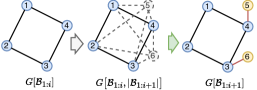
Figure 1: Example case where the equivariant graph transformation from $G[{\mathcal{B}}_{1:i}]$ to $G[{\mathcal{B}}_{1:i+1}]$ is impossible.

See proof in Apdx.§A.4. Theorem 3.1 indicates that no matter how powerful the equivariant network is, any structually equivalent elements have the same representation. Based on this theorem, we can easily show that there are many “bottleneck” cases where the targeted graph transformation cannot be achieved. Figure 1 shows a case where $G[{\mathcal{B}}_{1:}]$ is a 4-cycle, and the next target block contains two additional nodes, each with a single edge connecting to one of the nodes of $G[{\mathcal{B}}_{1:}]$. It is easy to see that nodes $1$–$4$ are all structurally equivalent, and so are nodes $5,6$ in the augmented case (middle). Hence, edges in $\{(5,i)|\forall i\in[1,4]\}$ are structurally equivalent (also $\{(6,i)|\forall i\in[1,4]\}$). Similarly, $\forall i\in[1,4],$ edge $(5,i)$ and $(6,i)$ are structurally equivalent. Combining all cases, edges in $\{(j,i)|\forall i\in[1,4],j\in\{5,6\}\}$ are structurally equivalent. Theorem 3.1 states that all these edges would have the same prediction with any equivariant model, hence making the target $G[{\mathcal{B}}_{1:i+1}]$ not achievable.

The Magic of Annealing/Randomness. In Figure 1 we showed that a graph with many automorphisms cannot be transformed to a target graph with fewer automorphisms. We hypothesize that a graph with lower “energy” is hard to be transformed to a graph with higher “energy” with equivariant networks. There exist some definitions and discussion of graph energy (Gutman et al., 2009; Balakrishnan, 2004) based on symmetry and eigen-information to measure graph complexity, where graphs with more symmetries have lower energy. The theoretical characterization of the conditions for successful graph transformation is a valuable direction, which we leave for future work to investigate.

Based on the above hypothesis, to achieve a successful transformation of a graph into a target graph, it is necessary to increase its energy. Since graphs with fewer symmetries exhibit higher energy levels, our approach involves introducing random noise to both nodes and edges. Our approach of elevating the energy level, followed by its reduction to attain desired target properties, mirrors the annealing process.

Diffusion. This further motivates us to use denoising diffusion to model $p_{\theta}({\mathbf{x}}\ |\ G\big{[}{\mathcal{B}}_{1:i-1},|{\mathcal{B}}_{i}|\big{]})$: it naturally injects noise in the forward process, and its backward denoising process is the same as annealing. What is more, we can achieve the permutation-invariant property for $p_{\theta}\Big{(}G[{\mathcal{B}}_{1:i}]\setminus G[{\mathcal{B}}_{1:i-1}]\ \Big{|}\ G[{\mathcal{B}}_{1:i-1}]\Big{)}$, based on Proposition 1 in (Xu et al., 2022). Finally, as we have analyzed, this yields $p_{\theta}(G)$ in Eq. (12) to be permutation-invariant.

3.4 Pard: Autoregressive Denoising Diffusion

To summarize, we present Pard, the first permutation-invariant autoregressive diffusion model that integrates AR with denoising diffusion. Pard relies on a unique, permutation equivariant structural partial order $\phi$ (Algo. 1) to decompose the joint graph probability to the product of simpler conditional probabilities, based on Eq. (12). Each block’s conditional probability is modeled with the product of a conditional block size probability and a conditional block enlargement probability as in Eq. (13), where the conditional block enlargement probability for every block is a shared discrete denoising diffusion model as described in §3.1. Figure 2 illustrates Pard’s two parts : block-wise AR and local denoising diffusion at each AR step.

Notice that there are two tasks in Eq. (13); one for predicting the next block’s size, and the other for predicting the next block’s nodes and edges with diffusion. These two tasks can be trained together with a single network, although for better performance we use two different networks. For each block’s diffusion model, we set the maximum time steps to 40 without much tuning.

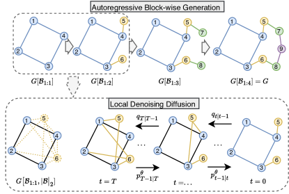
Figure 2: Pard integrates the autoregressive method with diffusion modeling. (top) Pard decomposes the joint probability into a series of block-wise enlargements, where each block’s conditional distribution is captured with a shared discrete diffusion (bottom).

Training and Inference Algorithm. We provide the training and inference algorithms for Pard in Apdx.§A.5. Specifically, Algo. 2 is used to train each next block’s size prediction model; Algo. 3 is used to train the shared diffusion for block conditional probabilities; and Algo. 4 presents the generation steps.

4 Architecture Improvement

Pard is a general framework that can be combined with any equivariant network. Nevertheless, we would like an equivariant network with enough expressiveness to process symmetries inside the generated blocks for modeling the next block’s conditional probability. While there are many expressive GNNs like subgraph GNNs (Bevilacqua et al., 2022; Zhao et al., 2022a) and higher-order GNNs (Zhao et al., 2022b; Morris et al., 2022), PPGN (Maron et al., 2019) is still a natural choice that models edge (2-tuple) representations directly with 3-WL expressivity and $O(n^{3})$ complexity in graph size. However, PPGN’s memory cost is relatively high for many datasets.

4.1 Efficient and Expressive Higher-order Transformer

To enhance the memory efficiency of Probabilistic Graph Neural Networks (PPGN) while maintaining the expressiveness equivalent to the 3-Weisfeiler-Lehman (3-WL) test, we introduce a hybrid approach that integrates Graph Transformers with PPGN. Graph Transformers operate on nodes as the fundamental units of representation, offering better scalability and reduced memory consumption compared to PPGN, while utilizing edges as their primary representation units and therefore incur significantly higher memory requirements. However, the expressiveness of Graph Transformers (without position encoding) is limited to the 1-WL test (Cai et al., 2023). By combining these two models, we can drastically decrease the size of edge representations while allocating larger hidden sizes to nodes. This synergistic approach not only substantially lowers the memory footprint but also enhances overall performance, leveraging the strengths of both architectures to achieve a balance between expressivity and efficiency. We provide the detailed design in Apdx.§A.6. Note that we use GRIT (Ma et al., 2023) as the transformer block.

4.2 Parallel Training with Causal Transformer

As shown in Eq. (12), for a graph $G$, there are $K_{B}$ conditional probabilities $p_{\theta}\Big{(}G[{\mathcal{B}}_{1:i}]\setminus G[{\mathcal{B}}_{1:i-1}]\ \Big{|}\ G[{\mathcal{B}}_{1:i-1}]\Big{)}$ being modeled by a shared diffusion model $f_{\theta}$. By default, these $K_{B}$ number of inputs $\{G[{\mathcal{B}}_{1:i-1}]\}_{i=1}^{K_{B}}$ are viewed as separate graphs and the network passing $f_{\theta}(G[{\mathcal{B}}_{1:i-1}])$ for different $i\in[1,K_{B}]$ are not shared. This leads to a scalability issue; in effect enlarging the dataset by roughly $K_{B}$ times and resulting in $K_{B}$ times longer training.

To minimize computational overhead, it is crucial to enable parallel training of all the $K_{B}$ conditional probabilities, and allow these processes to share representations, through which we can pass the full graph $G$ to the network $f_{\theta}$ only once and obtain all $K_{B}$ conditional probabilities. This is also a key advantage of transformers over RNNs. Transformers (GPTs) can train all next-token predictions simultaneously with representation sharing through causal masking, whereas RNNs must train sequentially. However, the default causal masking of GPTs is not applicable to our architecture as it contains both Transformer and PPGN.

To ensure representation sharing without risking information leakage, we first assign a “block ID” to every node and edge within graph $G$. Specifically, for every node and edge in $G[{\mathcal{B}}_{1:i}]\setminus G[{\mathcal{B}}_{1:i-1}]$, we assign the ID equal to $i$. To prevent information leakage effectively, it is crucial that any node and edge labeled with ID $i$ are restricted to communicate only with other nodes and edges whose ID is $\leq i$. Let ${\bm{A}},{\bm{B}}\in{\mathbb{R}}^{n\times n}$, and $\mathbf{x}\in{\mathbb{R}}^{n}$. There are mainly two non-elementwise operations in Transformer and PPGN that have the risk of leakage: the attention-vector product operation ${\bm{A}}\mathbf{x}$ of Transformer, and the matrix-matrix product operation ${\bm{A}}{\bm{B}}$ of PPGN. (We ignore the $d$ dimension of ${\bm{A}}$ and $\mathbf{x}$ as it does not affect the information leakage.)

Let ${\bm{M}}\in\{0,1\}^{n\times n}$ be a mask matrix, such that ${\bm{M}}_{i,j}=1$ if $\text{block\_ID}(i)\geq\text{block\_ID}(j)$ else 0. One can verify that

generalize ${\bm{A}}\mathbf{x}$ and ${\bm{A}}{\bm{B}}$ respectively and safely bypass information leakage. We use these operations in our network and enable representation sharing, along with parallel training of all $K_{B}$ blocks for denoising diffusion as well as next block size prediction. In practice, these offer more than 10$\times$ speed-up, and the parallel training allows Pard to scale to large datasets like MOSES (Polykovskiy et al., 2020).

5 Experiments

We evaluate Pard on 7 diverse benchmark datasets with varying sizes and structural properties, including both molecular (§5.1) and non-molecular/generic (§5.2) graph generation. A summary of the datasets is shown in Table 5.

5.1 Molecular Graph Generation

Datasets. We experiment with three different molecular datasets used across the graph generation literature: (1) QM9 (Ramakrishnan et al., 2014) (2) ZINC250k (Irwin et al., 2012), and (3) MOSES (Polykovskiy et al., 2020) that contains more than 1.9 million graphs. We use a 80%-20% train and test split, and among the train data we split additional 20% as validation. For QM9 and ZINC250k, we generate 10,000 molecules for stand-alone evaluation, and on MOSES we generate 25,000 molecules.

Baselines.  The literature has not been consistent in evaluating molecule generation on well-adopted benchmark datasets and metrics. Among baselines, DiGress (Vignac et al., 2023) stands out as the most competitive. We also compare to a list of many other baselines, where we report their performance values as sourced from the literature.

Metrics.  The literature has adopted a number of different evaluation metrics that are not consistent across datasets. Most common ones include Validity ($\uparrow$) (fraction of valid molecules without valency correction), Uniqueness ($\uparrow$) (frac. of valid molecules that are unique), and Novelty ($\uparrow$) (frac. of valid molecules that are not included in the training set).

For QM9, following earlier work (Vignac et al., 2023), we report additional evaluations w.r.t. Atom Stability ($\uparrow$) and Molecule Stability ($\uparrow$), as defined by (Hoogeboom et al., 2022b), whereas Novelty is not reported since QM9 contains small molecules that meet specific constraints, and generating novel molecules does not mean the network has accurately learned the data distribution.

Table 1: Generation quality on generic graphs. All metrics are based on generated-to-test set MMD distances, the lower the better. Top performance is in bold, and Runner-up is underlined.

	Community-small			Caveman			Cora			Breast
Model	Deg.	Clus.	Orbit	Deg.	Clus.	Orbit	Deg.	Clus.	Orbit	Deg.	Clus.	Orbit
GraphRNN	0.080	0.120	0.040	0.371	1.035	0.033	1.689	0.608	0.308	0.103	0.138	0.005
GRAN	0.060	0.110	0.050	0.043	0.130	0.018	0.125	0.272	0.127	0.073	0.413	0.010
EDP-GNN	0.053	0.144	0.026	0.032	0.168	0.030	0.093	0.269	0.062	0.131	0.038	0.019
GDSS	0.045	0.086	0.007	0.019	0.048	0.006	0.160	0.376	0.187	0.113	0.020	0.003
GraphArm	0.034	0.082	0.004	0.039	0.028	0.018	0.273	0.138	0.105	0.036	0.041	0.002
DiGress	0.047	0.041	0.026	0.019	0.040	0.003	0.044	0.042	0.223	0.152	0.024	0.008
Pard	0.023	0.071	0.012	0.002	0.047	0.00003	0.0003	0.003	0.0097	0.044	0.024	0.0003

On ZINC250k and MOSES, we also measure the Fréchet ChemNet Distance (FCD) ($\downarrow$) between the generated and the training samples, which is based on the embedding learned by ChemNet (Li et al., 2018a). For MOSES, there are three additional measures: Filter ($\uparrow$) score is the fraction of molecules passing the same filters as the test set, SNN ($\uparrow$) evaluates nearest neighbor similarity using Tanimoto Distance, and Scaffold similarity ($\uparrow$) analyzes the occurrence of Bemis-Murcko scaffolds (Polykovskiy et al., 2020).

Table 2: Generation quality on QM9 with explicit hydrogens.

Model	Valid. $\uparrow$	Uni. $\uparrow$	Atom.$\uparrow$	Mol. $\uparrow$
Dataset (optimal)	97.8	100	98.5	87.0
ConGress	86.7	98.4	97.2	69.5
DiGress (uniform)	89.8	97.8	97.3	70.5
DiGress (marginal)	92.3	97.9	97.3	66.8
DiGress (marg. + feat.)	95.4	97.6	98.1	79.8
Pard (no feat.)	97.5	95.8	98.4	86.1

Results.  Table 2 shows generation evaluation results on QM9, where the baseline results are sourced from (Vignac et al., 2023). Pard outperforms DiGress and variants that do not use any auxiliary features, in terms of Atom Stability and especially Validity and Molecule Stability, with slightly lower Uniqueness. What is notable is that Pard, without using any extra features, achieves a similar performance gap against DiGress that uses specialized extra features.

Table 3 shows Pard’s performance on ZINC250k, with baseline results carried over from (Kong et al., 2023) and (Yan et al., 2023). Pard achieves the best Uniqueness, stands out in FCD alongside SwinGNN (Yan et al., 2023), and is the runner-up w.r.t. Validity.

Table 3: Generation quality on ZINC250k.

Model	Validity $\uparrow$	FCD $\downarrow$	Uni. $\uparrow$	Model Size
EDP-GNN	82.97	16.74	99.79	0.09M
GraphEBM	5.29	35.47	98.79	-
SPECTRE	90.20	18.44	67.05	-
GDSS	97.01	14.66	99.64	0.37M
GraphArm	88.23	16.26	99.46	-
DiGress	91.02	23.06	81.23	18.43M
SwinGNN-L	90.68	1.99	99.73	35.91M
Pard	95.23	1.98	99.99	4.1M

Finally, Table 4 shows generation quality of Pard on the largest dataset MOSES. We mainly compare with DiGress and its variant ConGress, which has been the only general-purpose generative model in the literature that is not based on molecular fragments or SMILES strings. All baseline performances are sourced from (Vignac et al., 2023).

Table 4: Generation quality on MOSES. The top three methods use hard-coded rules, hence we do not highlight them.

Model	Val. ↑	Uni. ↑	Novel. ↑	Filters ↑	FCD ↓	SNN ↑	Scaf. ↑
VAE	97.7	99.8	69.5	99.7	0.57	0.58	5.9
JT-VAE	100	100	99.9	97.8	1.00	0.53	10.0
GraphINVENT	96.4	99.8	-	95.0	1.22	0.54	12.7
ConGress	83.4	99.9	96.4	94.8	1.48	0.50	16.4
DiGress	85.7	100	95.0	97.1	1.19	0.52	14.8
Pard	86.8	100	78.2	99.0	1.00	0.56	2.2

While the specialized models, excluding Pard and DiGress, have hard-coded rules to ensure high Validity, Pard outperforms those on several other metrics including FCD and SNN, and achives competitive performance on others. Again, it is notable here that Pard, without relying on any auxiliary features, achieves similarly competitive results as with DiGress which utilizes extra features.

5.2 Generic Graph Generation

Datasets.  We use four generic graph datasets with various structure and semantic: (1) Community-small (You et al., 2018), (2) Caveman (You, 2018), (3) Cora (Sen et al., 2008), and (4) Breast (Gonzalez-Malerva et al., 2011). We split each dataset into 80%-20% train-test, and randomly sample 20% of training graphs for validation. We generate the same number of samples as the test set.

Baselines.  We mainly compare against the latest general-purpose GraphArm (Kong et al., 2023), which reported DiGress (Vignac et al., 2023) and GDSS (Jo et al., 2022) as top two most competitive, along with several other baselines.

Metrics.  As with prior work (You et al., 2018), we measure generation quality using the maximum mean discrepancy (MMD) as a distribution distance between the generated graphs and the test graphs ($\downarrow$), as pertain to distributions of ($i$) Degree, ($ii$) Clustering coefficient, and ($iii$) occurrence count of all Orbits with 4 nodes.

Results. Table 1 provides the generation results of Pard against the baselines as sourced from (Kong et al., 2023). Pard shows outstanding performance achieving SOTA or close runner-up results, while none of the baselines shows as consistent performance across datasets and metrics.

6 Conclusion

We presented Pard, the first permutation-invariant autoregressive diffusion model. Pard decomposes the joint probability of a graph autoregressively into product of several block conditional probabilities relying on a unique and permutation equivariant structural partial order. All conditional probabilities are then modeled with a shared discrete diffusion. Pard can be trained in parallel on all blocks, and efficiently scales to millions of graphs. Pard achieves SOTA performance on molecular and non-molecular datasets without using any extra features. We expect Pard to serve as a cornerstone for generative foundation modeling on graphs.

Impact Statement

This paper presents work whose goal is to advance the field of Machine Learning. There are many potential societal consequences of our work, none which we feel must be specifically highlighted here.

Appendix A Appendix

A.1 Variational Lower Bound Derivation

$$\log \int q({\textnormal{G}}_{1:T}|{\textnormal{G}}_{0})\frac{p_{\theta}({\textnormal{G}}_{0:T})}{q({\textnormal{G}}_{1:T}|{\textnormal{G}}_{0})}d{\textnormal{G}}_{1:T}\geq\mathbb{E}_{q({\textnormal{G}}_{1:T}|{\textnormal{G}}_{0})}\big{[}\log p_{\theta}({\textnormal{G}}_{0:T})-\log q({\textnormal{G}}_{1:T}|{\textnormal{G}}_{0})\big{]}$$ (18)

$$=\mathbb{E}_{q({\textnormal{G}}_{1:T}|{\textnormal{G}}_{0})}\big{[}\log p_{\theta}({\textnormal{G}}_{0:T})+\sum_{t=1}^{T}\log\frac{p_{\theta}({\textnormal{G}}_{t-1}|{\textnormal{G}}_{t})}{q({\textnormal{G}}_{t}|{\textnormal{G}}_{t-1})}\big{]}$$

$$=\mathbb{E}_{q({\textnormal{G}}_{1:T}|{\mathbf{x}}_{0})}\big{[}\log p_{\theta}({\textnormal{G}}_{T})+\log\frac{p_{\theta}({\textnormal{G}}_{0}|{\textnormal{G}}_{1})}{q({\textnormal{G}}_{1}|{\textnormal{G}}_{0})}+\sum_{t=2}^{T}\log\frac{p_{\theta}({\textnormal{G}}_{t-1}|{\textnormal{G}}_{t})}{q({\textnormal{G}}_{t}|{\textnormal{G}}_{t-1},{\textnormal{G}}_{0})}\big{]}$$

$$=\mathbb{E}_{q({\textnormal{G}}_{1:T}|{\textnormal{G}}_{0})}\big{[}\log p_{\theta}({\textnormal{G}}_{T})+\log\frac{p_{\theta}({\textnormal{G}}_{0}|{\textnormal{G}}_{1})}{q({\textnormal{G}}_{1}|{\textnormal{G}}_{0})}+\sum_{t=2}^{T}\log\Bigg{(}\frac{p_{\theta}({\textnormal{G}}_{t-1}|{\textnormal{G}}_{t})}{q({\textnormal{G}}_{t-1}|{\textnormal{G}}_{t},{\textnormal{G}}_{0})}\cdot\frac{q({\textnormal{G}}_{t-1}|{\textnormal{G}}_{0})}{q({\textnormal{G}}_{t}|{\textnormal{G}}_{0})}\Bigg{)}\big{]}$$

$$=\mathbb{E}_{q({\textnormal{G}}_{1:T}|{\textnormal{G}}_{0})}\big{[}\log p_{\theta}({\textnormal{G}}_{T})+\log\frac{p_{\theta}({\textnormal{G}}_{0}|{\textnormal{G}}_{1})}{q({\textnormal{G}}_{1}|{\textnormal{G}}_{0})}+\log\frac{q({\textnormal{G}}_{1}|{\textnormal{G}}_{0})}{q({\textnormal{G}}_{T}|{\textnormal{G}}_{0})}+\sum_{t=2}^{T}\log\frac{p_{\theta}({\textnormal{G}}_{t-1}|{\textnormal{G}}_{t})}{q({\textnormal{G}}_{t-1}|{\textnormal{G}}_{t},{\textnormal{G}}_{0})}\big{]}$$

$$=\mathbb{E}_{q({\textnormal{G}}_{1:T}|{\textnormal{G}}_{0})}\big{[}\log p_{\theta}({\textnormal{G}}_{0}|{\textnormal{G}}_{1})+\log\frac{p_{\theta}({\textnormal{G}}_{T})}{q({\textnormal{G}}_{T}|{\textnormal{G}}_{0})}-\sum_{t=2}^{T}\log\frac{q({\textnormal{G}}_{t-1}|{\textnormal{G}}_{t},{\textnormal{G}}_{0})}{p_{\theta}({\textnormal{G}}_{t-1}|{\textnormal{G}}_{t})}\big{]}$$

$$=\underbrace{\mathbb{E}_{q({\textnormal{G}}_{1}|{\textnormal{G}}_{0})}\big{[}\log p_{\theta}({\textnormal{G}}_{0}|{\textnormal{G}}_{1})\big{]}}_{-\mathcal{L}_{1}(\theta)}-\sum_{t=2}^{T}\underbrace{\mathbb{E}_{q({\textnormal{G}}_{t}|{\textnormal{G}}_{0})}\big{[}D_{\mathrm{KL}}\big{(}q({\textnormal{G}}_{t-1}|{\textnormal{G}}_{t},{\textnormal{G}}_{0})||p_{\theta}({\textnormal{G}}_{t-1}|{\textnormal{G}}_{t}\big{)}\big{]}}_{\mathcal{L}_{t}(\theta)}-\text{const.}$$ (19)

Using Eq. (2), the first term can simplified as

$$\mathbb{E}_{q({\textnormal{G}}_{1}|{\textnormal{G}}_{0})}[\sum_{i}\log p_{\theta}({\mathbf{v}}^{i}_{0}|{\textnormal{G}}_{1})+\sum_{i,j}\log p_{\theta}({\mathbf{e}}^{i,j}_{0}|{\textnormal{G}}_{1})]\;,$$ (20)

and similarly, the $t$-th step loss $\mathcal{L}_{t}(\theta)$ is

$$\mathbb{E}_{q({\textnormal{G}}_{t}|{\textnormal{G}}_{0})}\big{[} \sum_{i}KL\big{(}q({\mathbf{v}}^{i}_{t-1}|{\mathbf{v}}^{i}_{t},{\mathbf{v}}^{i}_{0})\ ||\ p_{\theta}({\mathbf{v}}^{i}_{t-1}|{\textnormal{G}}_{t}\big{)}+$$

$$\sum_{i,j}KL\big{(}q({\mathbf{e}}^{i,j}_{t-1}|{\mathbf{e}}^{i,j}_{t},{\mathbf{e}}^{i,j}_{0})\ ||\ p_{\theta}({\mathbf{e}}^{i,j}_{t-1}|{\textnormal{G}}_{t}\big{)}\big{]}$$ (21)

A.2 Derivation of $q(x_{t-1}|x_{t},x_{0})$

First, define $\overline{Q}_{t|s}=Q_{s+1}...Q_{t}$. Note that $\overline{Q}_{t|0}=\overline{Q}_{t}$ and $\overline{Q}_{t|t-1}=Q_{t}$. Accordingly, we can derive the following two equalities.

$$q({\mathbf{x}}_{t}|{\mathbf{x}}_{t-1})=\text{Cat}({\mathbf{x}}_{t};\overline{Q}_{t}^{\top}{\mathbf{x}}_{t-1})\;$$ (22)

$$q({\mathbf{x}}_{t-1}|{\mathbf{x}}_{t},{\mathbf{x}}_{0}) =\frac{q({\mathbf{x}}_{t}|{\mathbf{x}}_{t-1})q({\mathbf{x}}_{t-1}|{\mathbf{x}}_{0})}{q({\mathbf{x}}_{t}|{\mathbf{x}}_{0})}=\frac{\text{Cat}({\mathbf{x}}_{t};Q_{t}^{\top}{\mathbf{x}}_{t-1})\text{Cat}({\mathbf{x}}_{t-1};\overline{Q}_{t-1}^{\top}{\mathbf{x}}_{0})}{\text{Cat}({\mathbf{x}}_{t};\overline{Q}_{t}^{\top}{\mathbf{x}}_{0})}$$

$$=\frac{{\mathbf{x}}_{t-1}^{\top}Q_{t}{\mathbf{x}}_{t}\cdot{\mathbf{x}}_{t-1}^{\top}\overline{Q}_{t-1}^{\top}{\mathbf{x}}_{0}}{{\mathbf{x}}_{t}^{\top}\overline{Q}_{t}^{\top}{\mathbf{x}}_{0}}={\mathbf{x}}_{t-1}^{\top}\frac{Q_{t}{\mathbf{x}}_{t}\odot\overline{Q}_{t-1}^{\top}{\mathbf{x}}_{0}}{{\mathbf{x}}_{t}^{\top}\overline{Q}_{t}^{\top}{\mathbf{x}}_{0}}=\text{Cat}({\mathbf{x}}_{t-1};\frac{Q_{t}{\mathbf{x}}_{t}\odot\overline{Q}_{t-1}^{\top}{\mathbf{x}}_{0}}{{\mathbf{x}}_{t}^{\top}\overline{Q}_{t}^{\top}{\mathbf{x}}_{0}})$$ (23)

A.3 Simplification of Transition Matrix

For any transition matrices $Q_{1},...,Q_{T}$, which however should be chosen such that every row of $\overline{Q}_{t}=\overline{Q}_{t|0}$ converge to the same known stationary distribution when $t$ becomes large (i.e. at $T$), let the known stationary distribution be ${\mathbf{m}}_{0}\sim\text{Cat}({\mathbf{m}}_{0};{\bm{m}})$. Then, the constraint can be stated as

$$\lim_{t\rightarrow T}\overline{Q}_{t}=\bm{1}{\bm{m}}^{\top}\;.$$ (24)

To achieve the desired convergence on nominal data (which is typical data type in edges and nodes of graphs), while keeping the flexibility of choosing any categorical stationary distribution ${\mathbf{m}}_{0}\sim\text{Cat}({\mathbf{m}}_{0};{\bm{m}})$, we define $Q_{t}$ as

$$Q_{t}=\alpha_{t}I+(1-\alpha_{t})\bm{1}{\bm{m}}^{\top}\;,$$ (25)

where $\alpha_{t}\in[0,1]$. This results in the accumulated transition matrix $\overline{Q}_{t|s}$ being equal to

$$\overline{Q}_{t|s}=\overline{\alpha}_{t|s}I+(1-\overline{\alpha}_{t|s})\bm{1}{\bm{m}}^{\top}\;\forall t>s\;,$$ (26)

where $\overline{\alpha}_{t|s}=\prod_{i=s+1}^{t}\alpha_{i}$. Note that $\overline{\alpha}_{t}=\overline{\alpha}_{t|0}=\overline{\alpha}_{t|s}\overline{\alpha}_{s}$. We achieve Eq. (24) by picking $\alpha_{t}$ such that $\lim_{t\rightarrow T}\overline{\alpha}_{t}=0$.

A.4 Proof of Theorem 3.1

We prove this for node case. For structurally equivalent edges, the analysis is the same. Assume node $i$ and node $j$ are structually equivalent, then we can find an automorphism $\sigma\in\text{Aut}(G)$ such that $\sigma(i)=j$. For any permutation ${\bm{P}}\in{\mathbb{P}}_{|G|}$ and an equivariant network $f$, we have

$$f({\bm{P}}\star G)={\bm{P}}\star f(G)$$ (27)

Replace ${\bm{P}}$ with $\sigma$, and using the fact that $\sigma\star G=G$. We can get

$$f(G)=f(\sigma\star G)=\sigma\star f(G)$$ (28)

Hence, we get $f(G)_{i}=f(G)_{j}$, that is two nodes $i$ and $j$ have the same representation.

A.5 Algorithms of Training and Generation

Algorithm 2 Train blocksize distribution $p_{\theta}\big{(}|{\mathcal{B}}_{i}|\ \big{|}\ G[{\mathcal{B}}_{1:i-1}]\big{)}$

1:  Input: $G$, maximum hop $K_{h}$, a network $f_{\theta}$ that takes a graph as input and output graph wise prediction.

2:  Get structural partial order function $\phi$ of $G$ from Algo.1.

3:  Using $\phi$ to get the sequence of node blocks $[{\mathcal{B}}_{1},...,{\mathcal{B}}_{K_{B}}]$ for $G$.

4:  Minimize $\sum_{i=1}^{K_{B}}\text{CrossEntropy}(f_{\theta}(G[{\mathcal{B}}_{i}]),|{\mathcal{B}}_{i+1}|)$, with $|{\mathcal{B}}_{K_{B}+1}|=0$

Algorithm 3 Train denoising diffusion for distribution $p_{\theta}\Big{(}G[{\mathcal{B}}_{1:i}]\setminus G[{\mathcal{B}}_{1:i-1}]\ \Big{|}\ G[{\mathcal{B}}_{1:i-1}]\cup\emptyset[{\mathcal{B}}_{1:i}]\Big{)}$

1:  Input: $G$, max time T, maximum hop $K_{h}$, a network $f_{\theta}$ that inputs a graph and outputs nodes and edges predictions.

2:  Get structural partial order function $\phi$ of $G$ from Algo.1.

3:  Using $\phi$ to get the sequence of node blocks $[{\mathcal{B}}_{1},...,{\mathcal{B}}_{K_{B}}]$ for $G$.

4:  Sample $t\sim U(1,...,T)$

5:  for $i=1,...,K_{B}$ do

6:     $M\leftarrow$ indice mask of $G[{\mathcal{B}}_{1:i}]\setminus G[{\mathcal{B}}_{1:i-1}]$

7:     Sample a noise graph $\tilde{G}[{\mathcal{B}}_{1:i}]$ from $q_{t|0}(G[{\mathcal{B}}_{1:i}])$ according to Eq. (5)

8:     $\tilde{G}[{\mathcal{B}}_{1:i}]\leftarrow M\odot\tilde{G}[{\mathcal{B}}_{1:i}]+(1-M)\odot G[{\mathcal{B}}_{1:i}]$

9:     $X\leftarrow f_{\theta}(\tilde{G}[{\mathcal{B}}_{1:i}])\odot M$

10:     $Y\leftarrow G[{\mathcal{B}}_{1:i}]\odot M$

11:     $l_{i}\leftarrow\mathcal{L}_{t}(X,Y)+0.1*\mathcal{L}_{t}^{CE}(X,Y)$, using $\mathcal{L}_{t}$ in Eq. (3) and $\mathcal{L}_{t}^{CE}$ in Eq. (3.1).

12:  end for

13:  Minimize $\sum_{i=1}^{K_{B}}l_{i}$.   (The for loop can be parallelized. )

Algorithm 4 Generation

1:  Input: blocksize model $g_{\varphi}$, diffusion model $f_{\theta}$; first blocksize distribution from TrainSet.

2:  $G\leftarrow\emptyset$; $i\leftarrow 1$

3:  Sample $n$ from the first block’s size distribution.

4:  while $n>0$ do

5:     Add a new block ${\mathcal{B}}_{i}$ with $n$ nodes into $G$

6:     $M\leftarrow$ indice mask of $G[{\mathcal{B}}_{1:i}]\setminus G[{\mathcal{B}}_{1:i-1}]$

7:     $\tilde{G}\leftarrow$ For nodes and edges within $M$, sample from noise ${\bm{m}}_{n}$ and ${\bm{m}}_{e}$.

8:     for $j=1:T$ do

9:        p $\leftarrow f_{\theta}(\tilde{G})$

10:        $S\leftarrow$ Sample according to p

11:        $\tilde{G}\leftarrow M\odot S+(1-M)\odot\tilde{G}$

12:     end for

13:     $G\leftarrow\tilde{G}$

14:     $n\leftarrow$ Sample from $g_{\varphi}(G)$

15:     $i\leftarrow i+1$

16:  end while

17:  Return: $G$

A.6 Visualization of the PPGN-Transformer Block

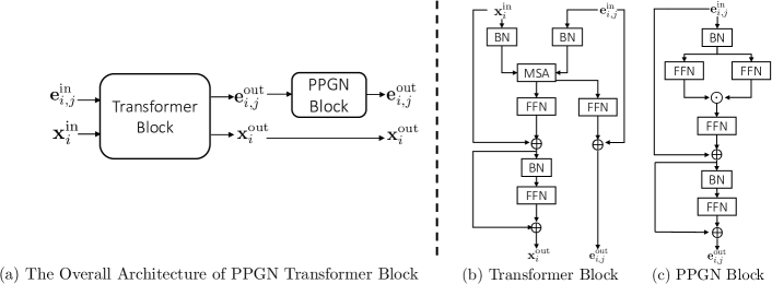
Figure 3: The Architecture of the PPGN-Transformer Block. In (b) and (c) we provide illustrations of how edge and node features are processed through Transformer and PPGN blocks.

A.7 Experiment Details

Table 5: Dataset summary

Name	#Graphs	$|V|_{\text{avg}}$	$|E|_{\text{avg}}$
QM9	133,885	9	19
ZINC250k	249,455	23	50
MOSES	1,936,963	22	47
Community-S	200	15.8	75.5
Caveman	200	13.9	68.8
Cora	18,850	51.9	121.2
Breast	100	55.7	117.0

References

- Anand & Huang (2018) Anand, N. and Huang, P. Generative modeling for protein structures. Advances in neural information processing systems, 31, 2018.
- Austin et al. (2021) Austin, J., Johnson, D. D., Ho, J., Tarlow, D., and van den Berg, R. Structured denoising diffusion models in discrete state-spaces. Advances in Neural Information Processing Systems, 34:17981–17993, 2021.
- Balakrishnan (2004) Balakrishnan, R. The energy of a graph. Linear Algebra and its Applications, 387:287–295, 2004.
- Bevilacqua et al. (2022) Bevilacqua, B., Frasca, F., Lim, D., Srinivasan, B., Cai, C., Balamurugan, G., Bronstein, M. M., and Maron, H. Equivariant subgraph aggregation networks. In International Conference on Learning Representations, 2022.
- Bommasani et al. (2021) Bommasani, R., Hudson, D. A., Adeli, E., Altman, R., Arora, S., von Arx, S., Bernstein, M. S., Bohg, J., Bosselut, A., Brunskill, E., et al. On the opportunities and risks of foundation models. arXiv preprint arXiv:2108.07258, 2021.
- Bonifati et al. (2020) Bonifati, A., Holubová, I., Prat-Pérez, A., and Sakr, S. Graph generators: State of the art and open challenges. ACM computing surveys (CSUR), 53(2):1–30, 2020.
- Cai et al. (2023) Cai, C., Hy, T. S., Yu, R., and Wang, Y. On the connection between mpnn and graph transformer. International Conference on Machine Learning, 2023.
- Chen et al. (2021) Chen, X., Han, X., Hu, J., Ruiz, F., and Liu, L. Order matters: Probabilistic modeling of node sequence for graph generation. In International Conference on Machine Learning, pp. 1630–1639. PMLR, 2021.
- De et al. (2022) De, S., Bermudez-Edo, M., Xu, H., and Cai, Z. Deep generative models in the industrial internet of things: a survey. IEEE Transactions on Industrial Informatics, 18(9):5728–5737, 2022.
- De Cao & Kipf (2018) De Cao, N. and Kipf, T. Molgan: An implicit generative model for small molecular graphs. arXiv preprint arXiv:1805.11973, 2018.
- Fan et al. (2023) Fan, W., Liu, C., Liu, Y., Li, J., Li, H., Liu, H., Tang, J., and Li, Q. Generative diffusion models on graphs: Methods and applications. arXiv preprint arXiv:2302.02591, 2023.
- Gonzalez-Malerva et al. (2011) Gonzalez-Malerva, L., Park, J., Zou, L., Hu, Y., Moradpour, Z., Pearlberg, J., Sawyer, J., Stevens, H., Harlow, E., and LaBaer, J. High-throughput ectopic expression screen for tamoxifen resistance identifies an atypical kinase that blocks autophagy. Proceedings of the National Academy of Sciences, 108(5):2058–2063, 2011.
- Goyal et al. (2020a) Goyal, N., Jain, H. V., and Ranu, S. Graphgen: A scalable approach to domain-agnostic labeled graph generation. In Proceedings of The Web Conference 2020, pp. 1253–1263, 2020a.
- Goyal et al. (2020b) Goyal, N., Jain, H. V., and Ranu, S. Graphgen: A scalable approach to domain-agnostic labeled graph generation. In Proceedings of The Web Conference 2020, pp. 1253–1263, 2020b.
- Gutman et al. (2009) Gutman, I., Li, X., and Zhang, J. Graph energy. Analysis of Complex Networks: From Biology to Linguistics, pp. 145–174, 2009.
- Ho et al. (2020) Ho, J., Jain, A., and Abbeel, P. Denoising diffusion probabilistic models. Advances in Neural Information Processing Systems, 33:6840–6851, 2020.
- Hoogeboom et al. (2021) Hoogeboom, E., Nielsen, D., Jaini, P., Forré, P., and Welling, M. Argmax flows and multinomial diffusion: Learning categorical distributions. Advances in Neural Information Processing Systems, 34:12454–12465, 2021.
- Hoogeboom et al. (2022a) Hoogeboom, E., Gritsenko, A. A., Bastings, J., Poole, B., van den Berg, R., and Salimans, T. Autoregressive diffusion models. In International Conference on Learning Representations, 2022a. URL https://openreview.net/forum?id=Lm8T39vLDTE.
- Hoogeboom et al. (2022b) Hoogeboom, E., Satorras, V. G., Vignac, C., and Welling, M. Equivariant diffusion for molecule generation in 3D. In Chaudhuri, K., Jegelka, S., Song, L., Szepesvari, C., Niu, G., and Sabato, S. (eds.), Proceedings of the 39th International Conference on Machine Learning, volume 162 of Proceedings of Machine Learning Research, pp. 8867–8887. PMLR, 17–23 Jul 2022b. URL https://proceedings.mlr.press/v162/hoogeboom22a.html.
- Irwin et al. (2012) Irwin, J. J., Sterling, T., Mysinger, M. M., Bolstad, E. S., and Coleman, R. G. Zinc: a free tool to discover chemistry for biology. Journal of chemical information and modeling, 52(7):1757–1768, 2012.
- Jo et al. (2022) Jo, J., Lee, S., and Hwang, S. J. Score-based generative modeling of graphs via the system of stochastic differential equations. In International Conference on Machine Learning, pp. 10362–10383. PMLR, 2022.
- Kong et al. (2023) Kong, L., Cui, J., Sun, H., Zhuang, Y., Prakash, B. A., and Zhang, C. Autoregressive diffusion model for graph generation. In International Conference on Machine Learning, pp. 17391–17408. PMLR, 2023.
- Li et al. (2018a) Li, Y., Vinyals, O., Dyer, C., Pascanu, R., and Battaglia, P. Learning deep generative models of graphs. arXiv preprint arXiv:1803.03324, 2018a.
- Li et al. (2018b) Li, Y., Zhang, L., and Liu, Z. Multi-objective de novo drug design with conditional graph generative model. Journal of Cheminformatics, 10:1–24, 2018b.
- Liao et al. (2019) Liao, R., Li, Y., Song, Y., Wang, S., Hamilton, W., Duvenaud, D. K., Urtasun, R., and Zemel, R. Efficient graph generation with graph recurrent attention networks. Advances in neural information processing systems, 32, 2019.
- Ma et al. (2023) Ma, L., Lin, C., Lim, D., Romero-Soriano, A., Dokania, K., Coates, M., H.S. Torr, P., and Lim, S.-N. Graph Inductive Biases in Transformers without Message Passing. In Proc. Int. Conf. Mach. Learn., 2023.
- Maron et al. (2019) Maron, H., Ben-Hamu, H., Serviansky, H., and Lipman, Y. Provably powerful graph networks. Advances in neural information processing systems, 32, 2019.
- Morris et al. (2022) Morris, C., Rattan, G., Kiefer, S., and Ravanbakhsh, S. Speqnets: Sparsity-aware permutation-equivariant graph networks. In International Conference on Machine Learning, pp. 16017–16042. PMLR, 2022.
- Niu et al. (2020) Niu, C., Song, Y., Song, J., Zhao, S., Grover, A., and Ermon, S. Permutation invariant graph generation via score-based generative modeling. In International Conference on Artificial Intelligence and Statistics, pp. 4474–4484. PMLR, 2020.
- Polykovskiy et al. (2020) Polykovskiy, D., Zhebrak, A., Sanchez-Lengeling, B., Golovanov, S., Tatanov, O., Belyaev, S., Kurbanov, R., Artamonov, A., Aladinskiy, V., Veselov, M., Kadurin, A., Johansson, S., Chen, H., Nikolenko, S., Aspuru-Guzik, A., and Zhavoronkov, A. Molecular Sets (MOSES): A Benchmarking Platform for Molecular Generation Models. Frontiers in Pharmacology, 2020.
- Ramakrishnan et al. (2014) Ramakrishnan, R., Dral, P. O., Rupp, M., and Von Lilienfeld, O. A. Quantum chemistry structures and properties of 134 kilo molecules. Scientific data, 1(1):1–7, 2014.
- Sen et al. (2008) Sen, P., Namata, G., Bilgic, M., Getoor, L., Galligher, B., and Eliassi-Rad, T. Collective classification in network data. AI magazine, 29(3):93–93, 2008.
- Shi* et al. (2020) Shi*, C., Xu*, M., Zhu, Z., Zhang, W., Zhang, M., and Tang, J. Graphaf: a flow-based autoregressive model for molecular graph generation. In International Conference on Learning Representations, 2020. URL https://openreview.net/forum?id=S1esMkHYPr.
- Simonovsky & Komodakis (2018) Simonovsky, M. and Komodakis, N. Graphvae: Towards generation of small graphs using variational autoencoders. In International conference on artificial neural networks, pp. 412–422. Springer, 2018.
- Sohl-Dickstein et al. (2015) Sohl-Dickstein, J., Weiss, E., Maheswaranathan, N., and Ganguli, s. Deep unsunpervised learning using nonequilibrium thermodynamics. In International Conference on Machine Learning, pp. 2256–2265. PMLR, 2015.
- Song & Ermon (2019) Song, Y. and Ermon, S. Generative modeling by estimating gradients of the data distribution. Advances in neural information processing systems, 32, 2019.
- Song et al. (2021) Song, Y., Sohl-Dickstein, J., Kingma, D. P., Kumar, A., Ermon, S., and Poole, B. Score-based generative modeling through stochastic differential equations. In International Conference on Learning Representations, 2021. URL https://openreview.net/forum?id=PxTIG12RRHS.
- Srinivasan & Ribeiro (2020) Srinivasan, B. and Ribeiro, B. On the equivalence between positional node embeddings and structural graph representations. In International Conference on Learning Representations, 2020. URL https://openreview.net/forum?id=SJxzFySKwH.
- Tong et al. (2021) Tong, X., Liu, X., Tan, X., Li, X., Jiang, J., Xiong, Z., Xu, T., Jiang, H., Qiao, N., and Zheng, M. Generative models for de novo drug design. Journal of Medicinal Chemistry, 64(19):14011–14027, 2021.
- Trinquier et al. (2021) Trinquier, J., Uguzzoni, G., Pagnani, A., Zamponi, F., and Weigt, M. Efficient generative modeling of protein sequences using simple autoregressive models. Nature communications, 12(1):5800, 2021.
- Vignac et al. (2023) Vignac, C., Krawczuk, I., Siraudin, A., Wang, B., Cevher, V., and Frossard, P. Digress: Discrete denoising diffusion for graph generation. In The Eleventh International Conference on Learning Representations, 2023. URL https://openreview.net/forum?id=UaAD-Nu86WX.
- Xu et al. (2022) Xu, M., Yu, L., Song, Y., Shi, C., Ermon, S., and Tang, J. Geodiff: A geometric diffusion model for molecular conformation generation. In International Conference on Learning Representations, 2022. URL https://openreview.net/forum?id=PzcvxEMzvQC.
- Yan et al. (2023) Yan, Q., Liang, Z., Song, Y., Liao, R., and Wang, L. Swingnn: Rethinking permutation invariance in diffusion models for graph generation. arXiv preprint arXiv:2307.01646, 2023.
- You (2018) You, J. Caveman Dataset. https://github.com/JiaxuanYou/graph-generation/blob/master/create_graphs.py, 2018. [Online; accessed 31-Jan-2024].
- You et al. (2018) You, J., Ying, R., Ren, X., Hamilton, W., and Leskovec, J. Graphrnn: Generating realistic graphs with deep auto-regressive models. In International conference on machine learning, pp. 5708–5717. PMLR, 2018.
- Zhang et al. (2021) Zhang, M., Li, P., Xia, Y., Wang, K., and Jin, L. Labeling trick: A theory of using graph neural networks for multi-node representation learning. Advances in Neural Information Processing Systems, 34:9061–9073, 2021.
- Zhao et al. (2022a) Zhao, L., Jin, W., Akoglu, L., and Shah, N. From stars to subgraphs: Uplifting any GNN with local structure awareness. In International Conference on Learning Representations, 2022a. URL https://openreview.net/forum?id=Mspk_WYKoEH.
- Zhao et al. (2022b) Zhao, L., Shah, N., and Akoglu, L. A practical, progressively-expressive gnn. Advances in Neural Information Processing Systems, 35:34106–34120, 2022b.