Logical Specifications-guided Dynamic Task Sampling
for Reinforcement Learning Agents

Abstract

Reinforcement Learning (RL) has made significant strides in enabling artificial agents to learn diverse behaviors. However, learning an effective policy often requires a large number of environment interactions. To mitigate sample complexity issues, recent approaches have used high-level task specifications, such as Linear Temporal Logic (LTL_f) formulas or Reward Machines (RM), to guide the learning progress of the agent. In this work, we propose a novel approach, called Logical Specifications-guided Dynamic Task Sampling (LSTS), that learns a set of RL policies to guide an agent from an initial state to a goal state based on a high-level task specification, while minimizing the number of environmental interactions. Unlike previous work, LSTS does not assume information about the environment dynamics or the Reward Machine, and dynamically samples promising tasks that lead to successful goal policies. We evaluate LSTS on a gridworld and show that it achieves improved time-to-threshold performance on complex sequential decision-making problems compared to state-of-the-art RM and Automaton-guided RL baselines, such as Q-Learning for Reward Machines and Compositional RL from logical Specifications (DIRL). Moreover, we demonstrate that our method outperforms RM and Automaton-guided RL baselines in terms of sample-efficiency, both in a partially observable robotic task and in a continuous control robotic manipulation task.

1 Introduction

Agents are now capable of learning optimal control behavior for a broad spectrum of tasks, ranging from Atari games (Gao and Wu 2021) to robotic manipulation tasks (Nguyen and La 2019), thanks to recent advancements in Reinforcement Learning (RL). Despite the progress made in RL, learning an optimal task policy using model-free RL techniques still suffers from sample complexity issues because of sparse reward settings and unknown transition dynamics (Lattimore, Hutter, and Sunehag 2013). These challenges further intensify in long-horizon settings, where the agent needs to perform a series of correct sequential decisions to achieve the goal. Additionally, certain tasks (such as - robot needs to make dinner only if it bought groceries in the afternoon) require the agent to encode and remember its episodic history (whether the groceries were bought) in order to solve the task effectively. To alleviate this issue in complicated tasks, several lines of work have explored representing the goal using an intricately shaped reward function that guides the agent toward the goal (Grzes 2017). However, generating such a reward function requires the human engineer to assign ‘importance’ weights to various aspects of the task, which is time consuming and assumes knowledge on which aspects of the task are important. Poorly engineered reward functions can lead to local optima, where the agent learns to satisfy only a subset of goals and ignores the rest.

Recent research has investigated representing the goal using high-level specification languages, such as finite-trace Linear Temporal Logic (LTL_f) (De Giacomo and Vardi 2013), Reward Machines (RM) (Icarte et al. 2022), SPECTRL (Jothimurugan, Alur, and Bastani 2019) that allow defining the goal of the task using a graphical representation of sub-tasks. The high-level objective is known before commencing the task, and the graphical representation allows the agent to achieve easier sub-goals initially, and build upon them to achieve complex goals. Encoding the task using a graphical structure allows us to tackle the problem in a Markovian manner by tracking the history as a part of the state space (Afzal et al. 2023), thereby allowing the agent to keep track of its episodic history. For instance, if the task for a robot is to reach kitchen and then make dinner, the graphical structure of the task obtained from the high-level specification allows the agent to reason whether it has reached the kitchen before it can commence its policy for making dinner.

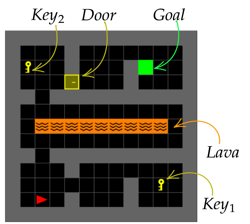
(a) Gridworld domain

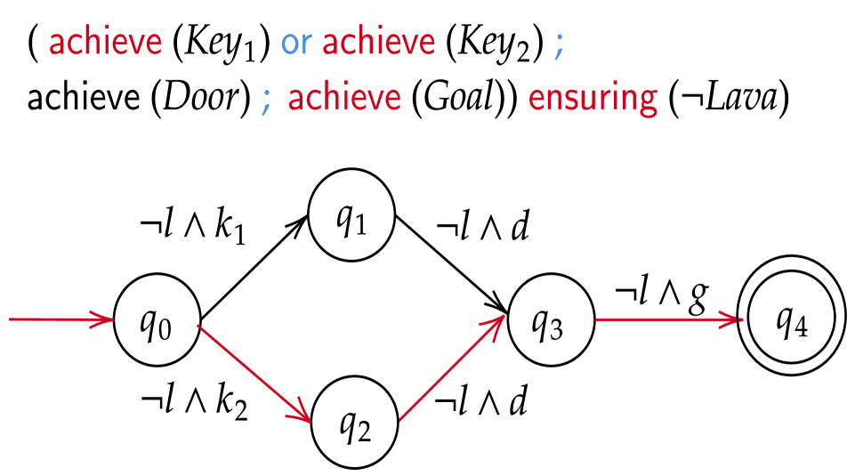
(b) SPECTRL formula and its corresponding DAG. The DAG excludes all self-loops and transitions to a sink state.

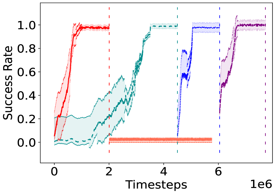
(c) Learning curve

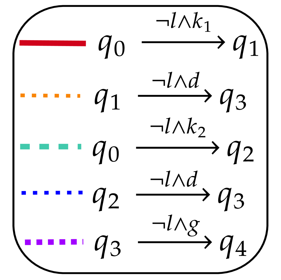
Figure 1: (a) Gridworld domain and descriptors. The agent (red triangle) needs to collect one of the keys and open the door to reach the goal; (b) The SPECTRL formula for the task and its DAG. Formulas $l$, $k_{1}$, $k_{2}$, $d$ and $g$ correspond to $Lava$, $Key_{1}$, $Key_{2}$, $Door$ and $Goal$ respectively; (c) Learning curves for individual sub-tasks (averaged over 10 trials) generated using LSTS. The path chosen by LSTS is highlighted in red in Fig.1(b)

RM approaches still require human guidance in defining the reward structure of the machine, which is dependent on knowing how much reward should be assigned for accomplishing each sub-goal. The process of designing the reward structure assumes that the human engineer is aware of how much should reward should the agent receive when it accomplishes the sub-goals in particular order. This assumption is infeasible in scenarios when the structure of the environment or the exact order in which the sub-goals must be achieved is unknown in advance. In contrast, our method does not require access to the reward structure.

Another method, Compositional RL from Logical Specifications (DiRL) (Jothimurugan et al. 2021) mitigates the reward assignment issue by using Dijkstra’s algorithm to determine which sub-tasks (edges) should be explored in the SPECTRL DAG graph (Jothimurugan, Alur, and Bastani 2019) in order to learn policies to reach nodes in the DAG that yield the highest success rate. DiRL requires the agent to learn RL policies for satisfying all outgoing edge propositions (each edge encodes a sub-task) from such nodes. However, this approach requires the agent to explore a sub-task for a manually specified number of interactions, which requires knowledge about the task complexity. DiRL ends up spending a lot of interactions learning unproductive policies as some sub-tasks can be unpromising, yet the agent has to spend the defined number of interactions learning a policy for the sub-task. Unlike  DiRL, our approach is sample-efficient as it finds unpromising sub-tasks based on the learning progress of the sub-tasks, and discards them; saving costly interactions and converging to a successful policy faster. This problem of minimizing the overall number of interactions while learning a set of successful policies is non-trivial as the problem equates to finding the shortest path in a graph whose true edge weights are unknown a priori (Szepesvári 2004). In our case, the edge weight denotes the total number of environmental interactions required by the agent to learn a successful policy for the sub-task encoded by the edge, in which the agent must induce a visit to a state where certain properties hold true. And, we can sample interactions for a sub-task only if we have a policy to reach the edge’s source node from the start node of the graph, making the learning process more sample-inefficient.

To address the above challenges, we present Logical Specifications-guided Dynamic Task Sampling (LSTS). We begin with a high-level objective represented using  SPECTRL specification formulas which can equivalently be represented using directed acyclic graphs (DAG) (Jothimurugan, Alur, and Bastani 2019). The DAG structure encodes memory, helping the agent understand what events of interest have occurred in the past, and which events must occur to reach the accepting states. Our key insight is to learn RL policies for sub-tasks defined using the edges of the DAG. Specifically, the agent transitions from the node $q$ to $p$ in the DAG when the propositional logic formula labeling the edge $(q,p)$ evaluates to true. We use the set of propositional logic formulas labeling the outgoing edges from a given node in DAG to define sub-tasks. The trajectory induced by a successful RL policy for the sub-task enables the agent’s high-level state in the DAG to transition from the source node to the destination node of the edge defining the sub-task. We employ an adaptive Teacher-Student learning strategy, where, (1) the Teacher agent uses its high-level policy along with exploration techniques to actively sample a sub-task for the Student agent to learn. The high-level policy considers the DAG representation and the Student agent’s expected performance on all the sub-tasks, aiming to satisfy the high-level objective in the fewest number of interactions, and (2) the Student agent interacts with the environment for a few steps (much fewer than the interactions required to learn a successful policy for the sub-task) while updating its low-level RL policy for the sampled sub-task. The Teacher observes the Student’s performance on these interactions and updates its high-level policy. Steps (1) and (2) continue alternately until the Student agent learns a set of successful policies that guide the agent to reach a goal state.

Running example: As an example, let us look at the environment shown in Fig. 1. The goal for the agent is to collect any of the two Keys, followed by opening the Door and then reaching the Goal while avoiding the Lava at all times. The task’s high-level objective ($\phi$) is represented using the SPECTRL formula and its corresponding DAG representation $\mathcal{G}_{\phi}$ in Fig. 1. The DAG does not contain information about the environment configuration, such as: the optimal number of interactions required to reach $Door$ from $Key_{1}$ are much higher compared to the interactions required to reach $Door$ from $Key_{2}$, making the $Key_{1}$ to $Door$ trajectory sub-optimal. Hence, it is crucial to prevent any additional interactions the agent spends in learning a policy for the sub-task defined by the edge $q_{1}\xrightarrow{\neg l\wedge d}q_{3}$ as the path $q_{0}\xrightarrow{\neg l\wedge k_{1}}q_{1}\xrightarrow{\neg l\wedge d}q_{3}\xrightarrow{\neg l\wedge g}q_{4}$ will always be sub-optimal. In our proposed approach LSTS, the Student agent begins with the aim of learning two distinct RL policies: $\pi_{1}$ for the task of visiting $Key_{1}$ and $\pi_{2}$ for the task of visiting $Key_{2}$, both avoiding $Lava$. The Teacher agent initially samples evenly from these two sub-tasks for the Student but later biases its sampling toward the sub-task on which the Student agent shows higher learning potential. Once the Student agent learns a successful policy for one of the sub-tasks (let’s say the learned policy $\pi_{1}^{*}$ corresponding to the sub-task defined by the transition $q_{0}\xrightarrow{\neg l\wedge k_{1}}q_{1}$), the Teacher does not sample that task anymore, identifies the next task(s) for the Student using the DAG representation, and appends them to the set of tasks it is currently sampling (in this case, the only next task is: $q_{1}\xrightarrow{\neg l\wedge d}q_{3}$). Since the Student agent only has access to the state distribution over $q_{0}$, it follows the trajectory given by $\pi_{1}^{*}$ to reach a state that lies in the set of states where the proposition $\neg Lava\wedge Key_{1}$ holds true before commencing its learning for the policy ($\pi_{3}$) for $q_{1}\xrightarrow{\neg l\wedge d}q_{3}$. If the Student agent learns the policies $\pi_{2}^{*}$ for satisfying the sub-task defined by $q_{0}\xrightarrow{\neg l\wedge k_{2}}q_{2}$ and $\pi_{4}^{*}$ for $q_{2}\xrightarrow{\neg l\wedge d}q_{3}$ before learning $\pi_{3}$, it effectively has a set of policies to reach the node $q_{3}$. Thus, the Teacher will now only sample the next task for the Student in the DAG representation $q_{3}\xrightarrow{\neg l\wedge g}q_{4}$, as learning RL policies for paths that reach $q_{3}$ are effectively redundant. This process continues iteratively until the Student agent learns a set of policies that reach the goal node ($q_{4}$) from the start node ($q_{0}$). The learning curves in Fig. 1 empirically validate the running example. As evident from the learning curves, the Student agent learns policies for the path $q_{0}\xrightarrow{\neg l\wedge k_{2}}q_{2}\xrightarrow{\neg l\wedge d}q_{3}\xrightarrow{\neg l\wedge g}q_{4}$ that produce trajectories to reach the goal node $q_{4}$ from the initial node $q_{0}$, without excessively wasting interactions on the unpromising sub-task $q_{1}\xrightarrow{\neg l\wedge d}q_{3}$. The dashed lines in Fig. 1 signify the interactions at which a task policy converged.

The dynamic task sampling strategy promotes LSTS to achieve sample-efficient learning on complex tasks by identifying unpromising tasks and discarding them, saving costly interactions. Our empirical results show that LSTS reduces environmental interactions by orders of magnitude compared to state-of-the-art Specifications-Guided RL Baseline DiRL, Reward Machine-based baselines QRM (Icarte et al. 2018), GSRS (Camacho et al. 2018), and curriculum learning baseline TSCL (Matiisen et al. 2020). We also evaluate LSTS^ct, a modified algorithm that further improves sample efficiency by continuing exploration on a new sub-task once a goal state for a sub-task is reached. We perform evaluation on two robotic navigation and manipulation tasks and demonstrate that LSTS reduces the number of interactions by orders-of-magnitude when compared to state-of-the-art automaton-guided RL baselines.

2 Related Work

Automaton-guided RL approaches utilize temporal logic-based language specifications to define tasks (Toro Icarte et al. 2018; Bozkurt et al. 2020; Xu and Topcu 2019; Alur et al. 2022). Separating policies for task sub-goals aids in abstracting knowledge that can be utilized in novel tasks (Icarte et al. 2018), without reliance on a dense reward function. Another technique is to shape the reward in proportion to the distance from the accepting node in the automaton (Camacho et al. 2018); however, this often leads to suboptimal reward settings. Augmenting the reward function with Monte Carlo Tree Search helps mitigate this issue (Velasquez et al. 2021). This approach requires the ability to plan-ahead in the environment, which is not always feasible. Automaton-guided RL has been used to aid navigational exploration for robotic domains (Cai et al. 2023) and for multi-agent settings (Hammond et al. 2021). Generating a curriculum given the high-level objective (Shukla et al. 2023) requires access to the Object-Oriented MDP (Diuk, Cohen, and Littman 2008), which cannot be obtained if environment details are not known in advance. DiRL interleaves high-level planning with RL to learn a policy for each edge, which overcomes challenges arising from poor representations (Jothimurugan et al. 2021). This approach becomes inefficient in terms of number of interactions, as it requires the agent to act for a predetermined number of interactions, even if learning the task does not show any promise. Unlike previous works, in this paper, we propose an logical specifications-guided dynamic task sampling approach that does not require access to the environment dynamics or the Reward Machine, and efficiently samples tasks that show promise toward the high-level objective, saving interactions on unpromising tasks.
Teacher-Student algorithms (Matiisen et al. 2020) have been previously studied in Curriculum Learning literature (Narvekar et al. 2020; Shukla et al. 2022, 2024) and in the Intrinsic Motivation literature (Oudeyer and Kaplan 2009). The idea is to have the Teacher propose those tasks to Student on which the Student shows most promise. This strategy helps Student learn simpler tasks first, transferring its knowledge to complex tasks. The technique reduces the overall number of interactions necessary to learn a successful policy. These approaches tend to optimize a curriculum to learn a single policy, which does not scale well to temporally-extended tasks. Instead, we propose an Logical Specifications-guided Teacher-Student learning strategy that learns a policies for promising automaton transitions, promoting sample-efficient training compared to the baselines.

3 Theoretical Framework

Episodic MDP. An episodic labeled Markov Decision Process (MDP) $M$ is a tuple $(\mathcal{S},\mathcal{A},P,R,\mathcal{S}_{0},\gamma,K,\mathcal{P},L)$, where $\mathcal{S}$ is the set of states, $\mathcal{A}$ is the set of actions, $P(s^{\prime}|s,a)$ denotes the transition probability of reaching state $s^{\prime}\in\mathcal{S}$ from $s\in\mathcal{S}$ using action $a\in\mathcal{A}$, $R:\mathcal{S}\times A\times\mathcal{S}\rightarrow\mathbb{R}$ is the reward function, $\mathcal{S}_{0}$ is the initial state distribution, $\gamma\in[0,1]$ is the discount factor, $K$ is the maximum number of interactions in any episode, $\mathcal{P}$ is a set of predicates, and $L:\mathcal{S}\rightarrow 2^{\mathcal{P}}$ is a labeling function that maps a state $s\in\mathcal{S}$ to a subset of predicates that are true in that state. In every interaction, the agent observes the current state $s$ and selects an action $a$ according to its policy function $\pi(a|s,\theta)$ with parameters $\theta$. The MDP transitions to a new state $s^{\prime}\in\mathcal{S}$ with probability $P(s^{\prime}\mid s,a)$. The agent’s goal is to learn an optimal policy $\pi^{*}$ that maximizes the discounted return $G_{0}=\sum^{K}_{k=0}\!\gamma^{k}\!R(s^{\prime}_{k},a_{k},s_{k})$ until the end of the episode, which occurs after at-most $K$ interactions.

High level specification language: In our framework, we adopt the specification language SPECTRL to articulate reinforcement learning tasks (Jothimurugan, Alur, and Bastani 2019). A specification $\phi$ in  SPECTRL is a logical formula applied to trajectories, determining whether a given trajectory $\zeta=(s_{0},s_{1},\ldots)$ successfully accomplishes a desired task. Mathematically, $\phi$ can be depicted as a function $\phi:\mathcal{Z}\to\mathbb{B}$, where $\mathbb{B}=\{\textsc{True},\textsc{False}\}$ and $\mathcal{Z}$ is the set of all trajectories.

Formally, a specification is defined over a set of atomic predicates $\mathcal{P}_{0}$. Each $p\in\mathcal{P}_{0}$ is associated with a function $f_{p}:S\to\mathbb{B}$. The agent’s MDP state $s$ satisfies $p$ (denoted by $s\models p$) when $f_{p}(s)=\texttt{True}$ (in other words, $p\subseteq L(s)$).

The set of predicates $\mathcal{P}$ comprises conjunctions and disjunctions of atomic predicates $\mathcal{P}_{0}$. A predicate $b\in\mathcal{P}$ follows the grammar $b::=p\mid(b_{1}\wedge b_{2})\mid(b_{1}\vee b_{2})$, where $p\in\mathcal{P}_{0}$. Each predicate $b\in\mathcal{P}$ corresponds to a function $f_{b}:S\to\mathbb{B}$ defined naturally over Boolean logic.

The syntax of SPECTRL specifications is given by

$$\phi::=\texttt{achieve}\>\>b\mid\phi_{1}\>\>\texttt{ensuring}\>\>b\mid\phi_{1};\phi_{2}\mid\phi_{1}\>\>\texttt{or}\>\>{\phi_{2}},$$

where $b\in\mathcal{P}$. Here, achieve and ensuring correspond to ‘eventually’ and ‘always’ operators in temporal logic. Each specification $\phi$ corresponds to a function $f_{\phi}:\mathcal{Z}\to\mathbb{B}$, and $\zeta\in\mathcal{Z}$ satisfies $\phi$ (denoted $\zeta\models\phi$) if $f_{\phi}(\zeta):=\textsc{True}$. The SPECTRL semantics for a finite trajectory $\zeta$ of length $t$ are:

$$\zeta\models\texttt{achieve}\>\>{b}\>\>\>\>\text{if}\>\>\>\exists\ i\leq t,~{}s_{i}\models b\>(\text{or}\>\>b\subseteq L(s))$$ (1)

$$\zeta\models\phi\>\>\texttt{ensuring}\>\>{b}\>\>\>\>\text{if}\>\>\>\exists\ i\leq t,~{}s_{i}\models b$$ (2)

$$\zeta\models\phi_{1};\phi_{2}\>\>\>\text{if}\>\>\>\exists\ i<t,~{}\zeta_{0:i}\models\phi_{1}\>\>\>\text{and}\>\>\>\zeta_{i+1:t}\models\phi_{2}$$ (3)

$$\zeta\models\phi_{1}\>\>\texttt{or}\>\>\phi_{2}\>\>\>\text{if}\>\>\>\zeta\models\phi_{1}\>\>\>\text{or}\>\>\>\zeta\models\phi_{2}$$ (4)

Intuitively, the condition $(1)$ signifies that the trajectory should eventually reach a state where the predicates $b$ hold true. The condition $(2)$ signifies that the trajectory should satisfy specification $\phi$ while always remaining in states where $b$ holds true. The condition $(3)$ signifies that the trajectory should sequentially satisfy $\phi_{1}$ and then $\phi_{2}$. The condition $(4)$ signifies that the trajectory should satisfy either $\phi_{1}$ or $\phi_{2}$. A trajectory $\zeta$ satisfies $\phi$ if there is a $t$ such that the prefix $\zeta_{0:t}$ satisfies $\phi$.

Furthermore, each SPECTRL specification $\phi$ is guaranteed to have an equivalent directed acyclic graph (DAG), called an abstract graph. An abstract graph $\mathcal{G}=(Q,E,q_{0},F,\beta,\mathcal{Z}_{safe},\kappa)$ is a directed acyclic graph (DAG) with nodes $Q$, (directed) edges $E\subseteq Q\times Q$, initial node $q_{0}\in Q$, final nodes $F\subseteq Q$, subgoal region map $\beta:Q\to 2^{\mathcal{S}}$ such that for each $q\in Q$, $\beta(q)$ is a subgoal region and safe trajectories $\mathcal{Z}_{safe}=\bigcup_{e\in E}\mathcal{Z}_{safe}^{e}$ where $\mathcal{Z}_{safe}^{e}\subseteq\mathcal{Z}_{f}$ denotes the safe trajectories for edge $e\in E$. Intuitively, $(Q,E)$ is a standard DAG, and $q_{0}$ and $F$ define a graph reachability problem for $(Q,E)$. Furthermore, $\beta$ and $\mathcal{Z}_{safe}$ connect $(Q,E)$ back to the original MDP $M$; in particular, for an edge $e=q\to q^{\prime}$, $\mathcal{Z}_{safe}^{e}$ is the set of trajectories in the MDP $M$ that can be used to transition from $\beta(q)$ to $\beta(q^{\prime})$. The function $\kappa$ labels each edge $e=q\rightarrow q^{\prime}$ with the predicates $b_{e}$ (labeled edge denoted as $e:=q\xrightarrow[]{b_{e}}q^{\prime}$). The agent transitions from $q$ to $q^{\prime}$ when the states $s_{i},s_{i+j}$ in the agent’s trajectory $\zeta$ satisfy $s_{i}\subseteq\beta(q)$ and $b_{e}\subseteq L(s_{i+j})$ and $j\geq 0$.

Given a SPECTRL specification $\phi$, we can construct an abstract graph $\mathcal{G}_{\phi}$ such that, for every trajectory $\zeta\in\mathcal{Z}$, we have $\zeta\models\phi$ if and only if $\zeta\models\mathcal{G}_{\phi}$. Thus, we can solve the reinforcement learning problem for $\phi$ by solving the reachability problem for $\mathcal{G}_{\phi}$. As described below, we leverage the structure of $\mathcal{G}_{\phi}$ in conjunction with reinforcement learning to do so. In summary, SPECTRL specifications provide a powerful and expressive means to define and evaluate reinforcement learning tasks. It allows users to specify complex conditions and requirements for successful task completion, enabling a nuanced approach to learning from specifications.

Problem Formulation. Given an MDP $M$ with unknown transition dynamics and a SPECTRL formula $\phi$ representing the high-level objective of the agent, let $\mathcal{G}_{\phi}$ be the DAG representing the language of $\phi$. Let $\mathsf{Paths}(q,X)$ be the set of all paths in the DAG originating in $q$ and terminating at a node in $X\subseteq Q$. The aim of this work is to learn a set of policies $\pi_{i}^{*}$, $i=0,\ldots,n-1$, with the following three properties: (i) Following $\pi_{0}^{*}$ results in a trajectory in the MDP that induces a transition from $q_{0}$ to some state $q_{1}\in Q$ in the DAG, following $\pi_{1}^{*}$ results in a trajectory in MDP that induces a transition from $q_{1}$ to some state $q_{2}\in Q$ in the DAG, and so on. (ii) The resulting path $q_{0}q_{1}\ldots q_{n}$ in the DAG terminates at a final node, i.e., $q_{n}\in F$, with probability greater than a given threshold, $\eta\in(0,1)$. (iii) The total number of environmental interactions spent in exploring and learning sub-task policies are minimized.

4 Methodology

Sub-task definiton: Given the DAG $\mathcal{G}_{\phi}$ representing the language of $\phi$, we define a set of sub-tasks based on the edges of the DAG. Intuitively, given any MDP state $s\in\mathcal{S}$ and a DAG node $q\in Q$, a sub-task defined by an edge from node $q$ to $p\in Q$ defines a reach-avoid objective for the agent represented by the SPECTRL formula,

$${\mathsf{Task}(q,p)\!\!:=\!\!\texttt{achieve}(b_{(q,p)})\>\texttt{ensuring}\left(\bigwedge\limits_{r\in\mathsf{Sc}(q),r\neq p}\!\!\!\neg b_{(q,r)}\!\!\right)}$$

where $b_{(q,p)}$ is the propositional formula labeling the edge from $q$ to $p$ in the DAG and $\mathsf{Sc}(q)$ is the set of successors of node $q$ in DAG. For example, in Fig. 1, the propositional formula labeling the edge from $q_{0}$ to $q_{1}$ is $b_{(q_{0},q_{1})}=\neg l\land k_{1}$. When $e=(q,p)$, we use $\mathsf{Task}(e)$ instead of $\mathsf{Task}(q,p)$ and $b_{e}$ instead of $b_{(q,p)}$ for notational convenience.

Each sub-task $\mathsf{Task}(q,p)$ defines a problem to learn a policy $\pi_{(q,p)}^{*}$ such that, given any MDP state $s_{0}\in\mathcal{S}$, following $\pi_{(q,p)}^{*}$ results in a trajectory $s_{0}s_{1}\ldots s_{n}$ in MDP that induces the path $qq\ldots qp$ in the DAG. That is, the agent’s high-level DAG state remains at $q$ until it transitions to $p$. While constructing the set of sub-tasks, we omit transitions that lead to a ‘sink’ state (from which final states are unreachable).

Given the MDP $M$ with unknown transition dynamics and the SPECTRL objective, $\phi$, we first translate $\phi$ to its corresponding directed acyclic graphical (DAG) representation $\mathcal{G}_{\phi}=(Q,E,q_{0},F,\beta,\mathcal{Z}_{safe},\kappa)$. Next, we define the set of sub-tasks. For this, we consider the edges that lie on some path in the DAG from $q_{0}$ to some node in $F$. This is because any path that does not visit $F$ leads to a sink state from which the objective cannot be satisfied. Such edges is identified using breadth-first-search (Moore 1959).

LSTS Initialization: The algorithm for LSTS is described in Algo. 1. We begin by initializing the following (lines 2-4): (1) Set of: Active Tasks AT, Learned Tasks LT, Discarded Tasks DT; (2) A Dictionary $\Pi$ that maps a sub-task $\mathsf{Task}(e)$ corresponding to edge $e$ of DAG $\mathcal{G}_{\phi}$ to a RL policy $\pi_{e}$; (3) A Dictionary representing the Teacher Q-Values $Q$ by mapping $\mathsf{Task}(e)$ to a numerical value associated with $\mathsf{Task}(e)$.

Firstly, we convert $\mathcal{G}_{\phi}$ into an Adjacency Matrix $\mathcal{X}$ (line 6), and find the tasks corresponding to the set all the outgoing edges $\overline{E}_{q_{0}}\subseteq E$ from the initial node $q_{0}$ (line 7). Satisfying the edge’s predicates $b_{(q_{0},q_{1})}\in\kappa(\overline{E}_{q_{0}})$ represent a reachability sub-task $M^{\prime}$ where each goal state $s\in\mathcal{S}^{M^{\prime}}_{f}$ of $M^{\prime}$ satisfy the condition $b_{(q_{0},q_{1})}\subseteq L(s)$. The Student agent receives a positive reward for satisfying $b_{(q_{0},q_{1})}$ and a small negative reward at all other time steps. The state and action space, and the transition dynamics of $M^{\prime}$ are equivalent to $M$. To complete the sub-task, the Student agent must learn a RL policy $\pi_{(q,p)}^{*}$ that ensures a visit from $q$ to $p$ with probability greater than a predetermined threshold ($\eta$). Moreover, the policy must also avoid triggering unintended transitions in the DAG. For instance, while picking up $Key_{1}$, the policy must not inadvertently pick up $Key_{2}$.

Teacher-Student learning: We set the Teacher Q-Values for all the sub-tasks corresponding to edges in AT (i.e., tasks corresponding to $\overline{E}_{q_{0}}$) to zero (line 8). We formalize the Teacher’s goal of choosing the most promising sub-task as a Partially Observable MDP (Kaelbling, Littman, and Cassandra 1998), where the Teacher does not have access to the entire Student agent state but only to the Student agent’s performance on a sub-task (e.g. success rate or average returns), and as an action, chooses a sub-task $\mathsf{Task}(e)\in$ AT the Student agent should train on next. In this POMDP setting, each Teacher action has an Q-Value associated with it. Intuitively, higher Q-Values correspond to tasks on which the Student agent is more successful, and the Teacher should sample such tasks at a higher frequency to satisfy $\phi$ (reach a goal node) in fewest overall interactions.

(A) Given the Teacher Q-Values, we sample a sub-task $\mathsf{Task}(e)\in$ AT using the $\epsilon-$greedy exploration strategy (line 10), and (B) The Student agent trains on task $\mathsf{Task}(e)$ using the RL policy $\Pi[e]$ for ‘$x$’ interactions (line 11). In one Teacher timestep, the Student trains for $x$ environmental interactions. Here, $x<<$ total number of environmental interactions required by the Student agent to learn a successful RL policy for $\mathsf{Task}(e)$, since the aim is to keep switching to a sub-task that shows highest promise. (C) The Teacher observes the Student agent’s average return $g_{t}$ on these $x$ interactions, and updates its Q-Value for $\mathsf{Task}(e)$ (line 12):

$$Q[e]\leftarrow\alpha(g_{t})+(1-\alpha)Q[e]$$ (5)

where $\alpha$ is the Teacher learning rate, $g_{t}$ is the average Student agent return on $\mathsf{Task}(e)$ at the Teacher timestep $t$. As the learning advances, $g_{t}$ increases as $t$ increases, and hence we use a constant parameter $\alpha$ to tackle the non-stationary problem of a moving return distribution. Several other algorithms could be used for the Teacher strategy (e.g., UCB or Thomspson Sampling). Steps (A), (B), (C) continue successively until the policy for any $\mathsf{Task}(e)\in$AT task converges.

Sub-task convergence criteria: We define Student agent’s RL policy for $\mathsf{Task}(q,p)$ to be converged (line 13) if a trajectory $\zeta$ produced by the policy triggers the transition with probability Pr${}_{\zeta\in\mathcal{Z}}[\zeta\mbox{ satisfies}\>\mathsf{Task}(q,p)]\>\geq\>\eta$ and $\Delta(g_{t},g_{t-1})\><\>\tau$ where $\eta$ is the expected performance and $\tau$ is a small numerical value. Intuitively, a converged policy attains an average success rate $\geq\eta$ and has not improved further by maintaining constant average returns. Like all other RM and automaton-based approaches, we assume access to the labeling function $L$ to examine if the trajectory $\zeta$ satisfies the formula $b_{(q,p)}$ by checking if the final environmental state $s$ of the trajectory satisfies the condition $b_{(q,p)}\subseteq L(s)$. The sub-goal regions need not be disjoint, i.e., the same state $s$ can satisfy propositions for multiple DAG nodes. Once a policy for the $\mathsf{Task}(q,p)$ converges, we append $\mathsf{Task}(q,p)$ to the set of Learned Tasks LT and remove it from the set of Active Tasks AT (line 14). In order to ensure that the learned sub-task does not get sampled any further, we set the Teacher Q-value for this sub-task to $-\infty$ (line 15).

Discarding unpromising sub-tasks: Once we have a successful policy for the $\mathsf{Task}(q,p)$ (the transition $q\xrightarrow{b_{(q,p)}}p$), we determine the sub-tasks that can be discarded (line 16). We find the sub-tasks corresponding to edges that: (1) lie before $p$ in a path from $q_{0}$ to any $q\in F$, and, (2) do not lie in a path to $q\in F$ that does not contain $p$. Intuitively, if we already have a set of policies that can generate a successful trajectory to reach the node $p$, we do not need to learn policies for sub-tasks that ultimately lead only to $p$ (e.g., in Fig. 1 if we have successful policies for $\mathsf{Task}(q_{0},q_{2})$ and $\mathsf{Task}(q_{2},q_{3})$, we can discard $\mathsf{Task}(q_{0},q_{1})$ and $\mathsf{Task}(q_{1},q_{3})$). We add all such sub-tasks to the set of Discarded Tasks DT (line 17), and set the Teacher Q-values for all the discarded tasks to $-\infty$ to prevent them from being sampled for the Student agent (line 18). As an extension, in the limit, an optimal policy can be found by not completely discarding such sub-tasks, but rather biasing away from them so that they would still be explored.

Algorithm 1 LSTS ( $\mathcal{G}_{\phi},M,\eta,x$ )

Output: Set of learned policies : $\Pi^{*}$, Edge-Policy Dictionary $\mathcal{P}$

1:  Placeholder Initialization:

2:  Sets of: Active Tasks (AT) $\leftarrow\emptyset$; Learned Tasks (LT) $\leftarrow\emptyset$; Discarded Tasks (DT) $\leftarrow\emptyset$

3:  Edge-Policy Dictionary $\Pi:\mathsf{Task}(e)\rightarrow\pi$

4:  Teacher Q-Value Dictionary: $Q:\mathsf{Task}(e)\rightarrow-\infty$

5:  Algorithm:

6:  $\mathcal{X}\leftarrow$ Adjacency_Matrix $(\mathcal{G}_{\phi})$

7:  AT $\leftarrow$ AT $\cup$ $\{\mathsf{Tasks}(\mathcal{X}[q_{0}])\}$

8:  $\forall\>\mathsf{Task}(e)\in$ AT $:Q[e]=0$

9:  while True do

10:     $e\leftarrow$ Sample$(Q)$

11:     $\Pi[e],g\leftarrow$ Learn$(M,\mathcal{G}_{\phi},e,x,\mathcal{P})$

12:     Update_Teacher$(Q,e,g)$

13:     if Convergence($Q,e,g,\eta$) then

14:        $\Pi^{*}\leftarrow\Pi^{*}\cup\Pi[e]$ ; LT $\leftarrow$ LT $\cup\{\mathsf{Task}(e)\}$ ; AT $\leftarrow$ AT $\setminus\{\mathsf{Task}(e)\}$

15:        $Q[e]=-\infty$

16:        $\mathsf{Tasks}(\overline{E}_{DT})\leftarrow$ Discarded_Tasks$(\mathcal{X},e)$

17:        DT $\leftarrow$ DT $\cup\>\mathsf{Tasks}(\overline{E}_{DT})$

18:        $\forall\>\mathsf{Task}(\overline{e})\>\in\>\mathsf{Tasks}(\overline{E}_{DT}):\>Q[\overline{e}]=-\infty\>$

19:        $\overline{E}_{AT}\leftarrow$ Next_Tasks $(\mathcal{X},e,$ DT)

20:        if $|\mathsf{Tasks}(\overline{E}_{AT})|=0$ then

21:           break

22:        end if

23:        $\forall\>\mathsf{Task}(\overline{e})\>\in\>\mathsf{Tasks}(\overline{E}_{AT}):Q[\overline{e}]=0$

24:        AT$\leftarrow$ AT $\cup\>\mathsf{Tasks}(\overline{E}_{AT})$

25:     end if

26:  end while

27:  return $\Pi^{*},\Pi$

Traversing in the DAG until $\phi$ satisfied: Subsequently, we determine the next set of tasks $\mathsf{Tasks}(\overline{E}_{AT})$ in the DAG to add to the AT set (line 19). This is calculated by identifying sub-tasks corresponding to all the outgoing edges from $p$. Since the edge $e_{q,p}$ corresponds to the transition $q\xrightarrow{b_{(q,p)}}p$, we have a successful policy that can produce a trajectory that reaches a state where $b_{(q,p)}$ hold true, and $\mathsf{Tasks}(\overline{E}_{AT})$ corresponds to $\mathcal{X}[p]\setminus$DT (‘$\setminus$’ refers to set-minus) i.e., sub-tasks corresponding to all the outgoing edges from $p$ that do not lie in the DT set.

After identifying $\mathsf{Tasks}(\overline{E}_{AT})$, we set Teacher Q-values for all $\mathsf{Task}(\overline{e})\in\mathsf{Tasks}(\overline{E}_{AT})$ to $0$ so that the Teacher will sample these tasks (line 23). In our episodic setting, the episode always starts from a state $s\sim\mathcal{S}_{0}$ where the propositions for $q_{0}$ hold true, and if the current sampled sub-task is $\mathsf{Task}(p,r)$, the agent follows a trajectory using learned policies from $\Pi^{*}$ to reach a state where the propositions for reaching DAG node $p$ hold true (i.e., $s\in\beta(p)$). The agent then attempts learning a separate policy for $\mathsf{Task}(p,r)$.

The above steps (lines 9-26) go on iteratively until $|\mathsf{Tasks}(\overline{E}_{AT})|=\emptyset$. This indicates we have no further tasks to add to our sampling strategy, and we have reached a node $q\in F$. Thus, we break from the while loop (line 21) and return the set of learned policies $\Pi^{*}$, and edge-policy dictionary $\Pi$ (line 27). From $\Pi$ and $\Pi^{*}$, we get an ordered list of policies $\Pi^{*}_{list}=[\pi_{(q_{1},q_{2})},\pi_{(q_{2},q_{3})},\ldots,\pi_{(q_{k-1},q_{k})}]$ such that sequentially following $\pi\in\Pi^{*}_{list}$ generates trajectories that satisfy the SPECTRL objective $\phi$ .
Guarantee: Given the ordered list of policies $\Pi^{*}_{list}$, we can generate a trajectory $\zeta$ in the task $M$ with Pr${}_{\zeta\in\mathcal{Z}}[\zeta\mbox{ satisfies }\phi]\geq\eta$ (Details in Appendix B).

5 Experimental Results

We aim to answer the following questions: (Q1) Does LSTS yield sample efficient learning compared to state-of-the-art baselines? (Q2) After reaching a sub-task goal state, can we sample a new sub-task to continue training and improve sample efficiency? (Q3) Does LSTS yield sample efficient learning for complex robotic tasks with partially observable or continuous control settings? (Q4) How does LSTS scale to complex search-and-rescue scenarios?

5.1 LSTS - Gridworld Domain

To answer (Q1), we evaluated LSTS on a Minigrid (Chevalier-Boisvert, Willems, and Pal 2018) inspired domain with the SPECTRL objective:

$$\phi^{grid}_{f}:=(\texttt{achieve}(k_{1})\>\texttt{or achieve}(k_{2});\\ \texttt{achieve}(d);\>\texttt{achieve}(g))\texttt{ensuring}(\neg l)$$ (6)

Approach	$\#$ Interactions
(Mean $\pm$ SD)	Success Rate
(Mean $\pm$ SD)
LSTSct	$(5.75\pm 0.38)\times 10^{6}$	$0.96\pm 0.02$
LSTS	$(6.12\pm 0.25)\times 10^{6}$	$0.95\pm 0.01$
DiRLc	$(7.97\pm 0.46)\times 10^{6}$	$0.95\pm 0.03$
DiRL	$(9.62\pm 0.42)\times 10^{6}$	$0.94\pm 0.01$
QRM	$5\times 10^{7}$	$0.05\pm 0.04$
GSRS	$5\times 10^{7}$	$0\pm 0$
TSCL	$5\times 10^{7}$	$0\pm 0$
LFS	$5\times 10^{7}$	$0\pm 0$

Table 1: Table comparing $\#$interactions $\&$ success rate.
LSTS (highlighted) outperfomed all baselines

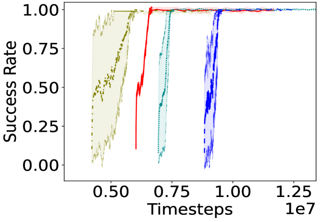
Figure 2: Averaged over 10 trials: Learning curves for approaches whose policies successfully converged.

where $k_{1},k_{2},d,g,l$ represent the atomic propositions $Key_{1},Key_{2},Door,Goal,Lava$ respectively. The environment and its $\phi$ are given in Fig. 1. Essentially, the agent needs to collect any of the Keys before heading to the Door. After toggling the Door open, the agent needs to visit the grid with the Goal. At all times, the agent needs to avoid the Lava object. We assume an episodic setting where an episode ends if the agent touches the Lava object, reaches the Goal or exhausts the number of allocated interactions.

This is a complex problem as the agent needs to perform a series of correct actions to satisfy $\phi^{grid}_{f}$. The agent has access to three navigation actions: move forward, rotate left and rotate right. The agent can also perfom: pick-up action, which adds the Key to the agent’s inventory if it is facing the Key, drop places the Key in the next grid if Key is present in the inventory, and, toggle that toggles the Door (closed $\leftrightarrow$ open) only if the agent is holding the Key. In this experiment, we assume a fully-observable setting where the environmental state is a low-level image encoding of the state. For each cell in the grid, the low-level encoding returns an integer that describes the item occupying the grid, along with any additional information (e.g., the Door can be open or closed).

For the Student RL agent, we use PPO (Schulman et al. 2017), which works for discrete and continuous action spaces. We consider a standard actor-critic architecture with 2 convolutional layers followed by 2 fully connected layers. For LSTS, the reward function is sparse. The agent gets a reward of $(1-0.9\frac{(interactions\>taken)}{(interactions\>allocated)})$ if it achieves the goal in the sub-task, and a reward of $0$ otherwise. For sub-tasks, $interactions\>allocated=100$. The agent does not receive any negative rewards for hitting the $Lava$.
Baselines: We compare our LSTS method with six baseline approaches: learning from scratch (LFS), Reward Machine-based (RM) baselines: GSRS (Camacho et al. 2018), QRM (Icarte et al. 2018); and Compositional RL from Logical Specifications (DiRL) (Jothimurugan et al. 2021). All the baselines are implemented using the RL algorithm (PPO), described above. GSRS assigns reward inversely proportional to the distance from the RM goal node. QRM employs a separate Q-function for each node in the RM, and DiRL uses Dijkstra’s algorithm (edge cost is the average RL policy success rate) to guide the agent in choosing a path from the specification graph. For the fifth baseline, we modify DiRL such that instead of manually specifying a limit on the number of interactions, which needs to be fine-tuned to suit the task, we stop learning a sub-task once it has reached the convergence criteria defined in Section 4. We call this modified baseline as DiRL^c. The sixth baseline (TSCL (Matiisen et al. 2020)) follows a curriculum learning strategy where the Teacher samples most promising task without the use of any automaton to guide the learning progress of the agent. (More details in Appendix C)

The results in Table 2 and Fig. 2 (averaged over 10 trials) show that LSTS reaches a successful policy quicker compared to all baselines. LSTS^ct is a modified version of LSTS and is described in Sec. 5.1. The learning curves in Fig. 2 have an offset on the x-axis to account for the interactions in the initial sub-tasks before moving on to the final task in the specification, signifying strong transfer (Taylor and Stone 2009). Our custom baseline, DiRL^c is more sample-efficient than DiRL, and both outperform other baselines, which do not learn a meaningful policy. We performed an unpaired t-test (Kim 2015) to compare LSTS against the best performing baselines at the end of $10^{7}$ training steps and we observed statistically significant results (95$\%$ confidence). Thus, LSTS not only achieves a better success rate, but also converges faster (statistical significance result details in Appendix D). Time-to-threshold metric is defined as the difference in number of interactions between two approaches to reach a desired performance (Narvekar et al. 2020). From Fig. 2, we see that the time-to-threshold between LSTS and the best-performing baseline DiRL^c is $1.85\times 10^{6}$ interactions for $95\%$ success rate.

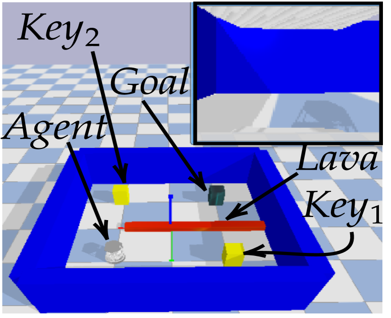
(a) TurtleBot domain

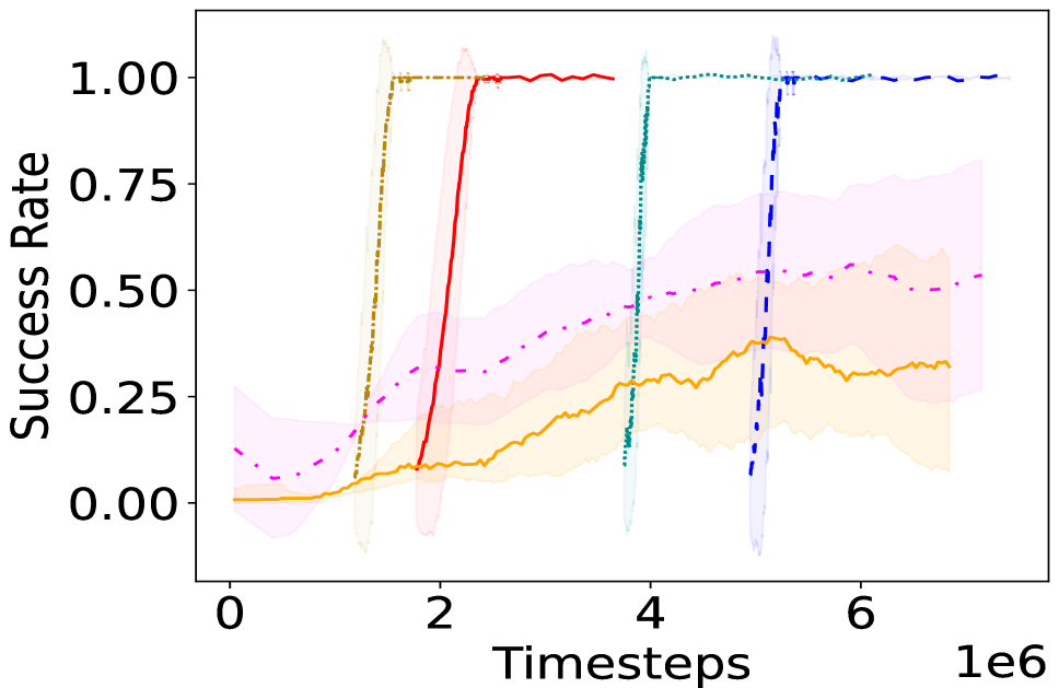
(b) Turtlebot results

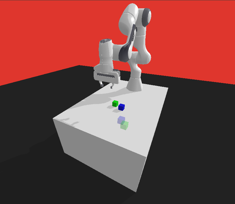
(c) Panda arm domain

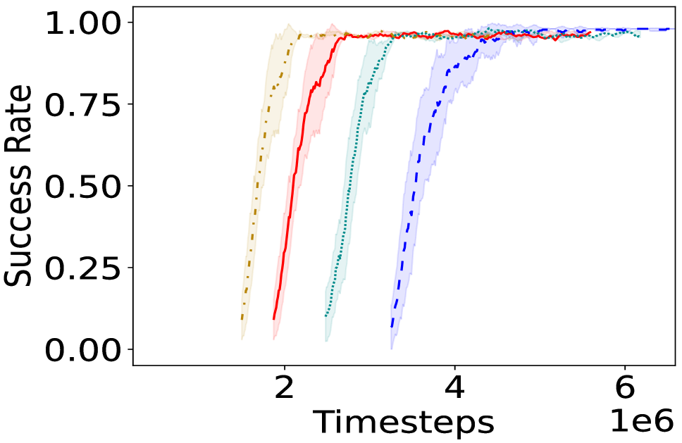
(d) Panda arm results

Figure 3: Learning curves (Averaged over 10 trials) for the two robotic domains.

LSTS^ct (LSTS + Cont. Training) - Gridworld Domain

In LSTS, while learning a policy for $\mathsf{Task}(q,p)$, we reinitialize the environment to a random initial environmental state $s\sim\mathcal{S}_{0}$ once the agent reaches a state where the propositions ($b_{(q,p)}$) hold true. To answer the question Q2, instead of resetting the environment after reaching such a state where $b_{(q,p)}$ hold true, we let the Teacher agent sample a task (let’s say $\mathsf{Task}(p,r)$) from the set $\mathcal{X}[p]\setminus$ DT, where $\mathcal{X}$ is the adjacency matrix for the graph, and DT is the set of Discarded Tasks, as defined in Algo. 1. This helps the agent continue its training by attempting to learn a policy $\pi_{(p,r)}$ for $\mathsf{Task}(p,r)$ while simultaneously learning a separate policy $\pi_{(q,p)}$ for $\mathsf{Task}(q,p)$. If the agent fails to satisfy $\mathsf{Task}(p,r)$, we reset the environment to state $s\sim\mathcal{S}_{0}$. Otherwise, the agent continues its training until its trajectory satisfies the high-level objective $\phi$. We call this approach LSTS^ct (Detailed algo in Appendix A). Results in Table 2 and Fig. 2 demonstrate that this approach improves sample efficiency by reducing the number of interactions required to learn a successful policy for the gridworld task, with a time-to-threshold metric of $3.7\times 10^{5}$ interactions as compared to LSTS.

5.2 LSTS and LSTS^ct - Robotic Domains

To answer (Q3), we test LSTS and LSTS^ct on two simulated robotic environments with high interaction cost. The task in Fig. 3 has the following SPECTRL objective:

$$\phi^{navigation}_{f}:=(\texttt{achieve}(Key_{1})\>\>\texttt{or}\>\>\texttt{achieve}(Key_{2});\\ \>\>\texttt{achieve}(Goal))\>\>\texttt{ensuring}(\neg Lava)$$ (7)

In this task, the agent (a simulated TurtleBot) needs to collect any of the keys (yellow blocks) present in a $[3m,3m]$ continuous environment before reaching the goal position (gray block). At all times, the agent needs to avoid the lava object (red wall) present in the center. The move forward (backward) action causes the robot to move forward (backward) by $0.1m$ and the robot rotates by $\pi/8$ radians with each rotate action. The pick-up and drop actions have effects similar to the gridworld domain. The robotic domain is more complex as objects can be placed at continuous locations. The agent receives an ego-centric image view of the environment (top-right corner of Fig. 3), which makes the task partially observable in nature and more complex to get a successful policy. The RL agent is described in Sec. 5.1.

The second environment (Fig. 3) consists of a simulated robotic arm pushing two objects to their target locations (Gallouédec et al. 2021) with the SPECTRL formula:

$$\phi^{manipulation}_{f}:=\texttt{achieve}(p_{1})\>\>;\>\>\texttt{achieve}(p_{2})$$ (8)

where $p_{1}$ and $p_{2}$ are the atomic propositions for ’push-object-1’, ‘push-object-2’. The robot has continuous action parameters for moving the arm and a binary gripper action (close/open). An episode begins with the two objects randomly initialized on the table, and the robotic arm has to push these two objects to its final location. The agent receives its current end-effector pose, positions and velocities of the two objects, and the desired goal position for the two objects. For this task, we use the Deep Deterministic Policy Gradient with Hindsight Experience Replay (DDPG-HER) (Andrychowicz et al. 2017) as our RL algorithm. DDPG-HER is implemented using the OpenAI baselines (Dhariwal et al. 2017). Both the robotic domains were modeled using PyBullet (Coumans and Bai 2021), and the reward structure for both the RL agents was sparse, similar to the one described in Sec. 5.1. The learning curves for the TurtleBot domain (Fig. 3) and the Panda arm domain (Fig 3) (averaged over 10 trials) are shown in Fig. 3 and Fig. 3 respectively. For both domains, LSTS outperforms all the baselines in terms of learning speed. LSTS^ct further speeds-up learning for both the robotic domains. The time-to-threshold between LSTS and the best performing baseline (our custom implementation) DIRL^c, is $2\times 10^{6}$ for the TurtleBot domain and $5\times 10^{5}$ for the Panda arm domain.

5.3 LSTS - Search and Rescue task

To demonstrate how LSTS performs when the plan length becomes deeper, we evaluated LSTS on a complex urban Search and Rescue domain with multi-goal objectives. In this domain, the agent acts in a grid setting where it needs to perform a series of sequential sub-tasks to accomplish the final goal of the task. The agent needs to open a door using a key, then collect a fire extinguisher to extinguish the fire, and then find and rescue stranded survivors. The order in which these individual sub-goals such as opening the door, rescuing the survivors, and extinguishing the fire are achieved does not matter. A fully-connected graph $\mathcal{G}_{phi}$ generated using the above mentioned high-level states consists of 24 distinct DAG paths. This is a multi-goal task as the agent needs to find the key to open the door, then extinguish fire and rescue survivors to reach the goal state (details in Appendix F). The results in Table 2 (averaged over 10 trials) show that LSTS reaches a successful policy quicker compared to the LFS, GSRS, QRM and TSCL. The overall number of interactions to learn a set of successful policies for satisfying the high-level goal objective are higher compared to the door key experiment because of the additional complexity of task. We observe that LSTS is able to accommodate the task and learn RL policies that satisfy the high-level goal objective.

Approach	$\#$ Interactions
(Mean $\pm$ SD)	Success Rate
(Mean $\pm$ SD)
LSTS	$(8.61\pm 0.12)\times 10^{6}$	$0.87\pm 0.04$
LFS	$5\times 10^{7}$	$0\pm 0$
GSRS	$5\times 10^{7}$	$0.05\pm 0.04$
QRM	$5\times 10^{7}$	$0.05\pm 0.04$
TSCL	$5\times 10^{7}$	$0\pm 0$

Table 2: Table comparing $\#$interactions $\&$ success rate for the Search and Rescue domain.

6 Conclusion

We proposed LSTS, a framework for dynamic task sampling for RL agents using the high-level SPECTRL objective coupled with the Teacher-Student learning strategy. Through experiments, we demonstrated that LSTS accelerates learning, converging to a desired success rate quicker as compared to other curriculum learning and automaton-guided RL baselines. LSTS^ct further improves sample efficiency by continuing exploration on a new sub-task once a goal state for a sub-task is reached. We also evaluate our approach on long-horizon complex robotic tasks where the state space is large and the actions are continuous. LSTS reduces training time without relying on human-guided dense reward function, accelerating learning when the high-level objective is available.

Limitations & Future Work: In certain cases, the SPECTRL objective can be novel and/or generating the labeling function can be infeasible. Our future plans involve expanding our framework to scenarios where obtaining a precise SPECTRL specification is challenging. As an extension, we would like to explore biasing away from sub-tasks rather than completely discarding them once the target node is reached, so in the limit, optimal policies can be obtained. We would also like to explore complex robotic and multi-agent scenarios with elaborate SPECTRL

References

- Afzal et al. (2023) Afzal, M.; Gambhir, S.; Gupta, A.; Trivedi, A.; and Velasquez, A. 2023. LTL-Based Non-Markovian Inverse Reinforcement Learning. In Proc. of the 2023 Intl. Conf. on Autonomous Agents and Multiagent Systems, 2857–2859.
- Alur et al. (2022) Alur, R.; Bansal, S.; Bastani, O.; and Jothimurugan, K. 2022. A framework for transforming specifications in reinforcement learning. In Principles of Systems Design. Springer.
- Andrychowicz et al. (2017) Andrychowicz, M.; Wolski, F.; Ray, A.; Schneider, J.; Fong, R.; Welinder, P.; McGrew, B.; Tobin, J.; and Pieter Abbeel, W., Zaremba. 2017. Hindsight experience replay. NeurIPS.
- Bozkurt et al. (2020) Bozkurt, A. K.; Wang, Y.; Zavlanos, M. M.; and Pajic, M. 2020. Control synthesis from linear temporal logic specifications using model-free reinforcement learning. In 2020 IEEE Intl. Conf. on Robotics and Automation (ICRA), 10349–10355. IEEE.
- Cai et al. (2023) Cai, M.; Aasi, E.; Belta, C.; and Vasile, C.-I. 2023. Overcoming Exploration: Deep Reinforcement Learning for Continuous Control in Cluttered Environments From Temporal Logic Specifications. IEEE RAL, 8(4): 2158–2165.
- Camacho et al. (2018) Camacho, A.; Chen, O.; Sanner, S.; and McIlraith, S. A. 2018. Non-Markovian rewards expressed in LTL: Guiding search via reward shaping. In GoalsRL, a workshop collocated with ICML/IJCAI/AAMAS.
- Chevalier-Boisvert, Willems, and Pal (2018) Chevalier-Boisvert, M.; Willems, L.; and Pal, S. 2018. Minimalistic Gridworld Environment for Gymnasium.
- Coumans and Bai (2021) Coumans, E.; and Bai, Y. 2021. PyBullet, a Python module for physics simulation for games, robotics and machine learning. http://pybullet.org. Accessed: 2023-04-02.
- De Giacomo and Vardi (2013) De Giacomo, G.; and Vardi, M. Y. 2013. Linear temporal logic and linear dynamic logic on finite traces. In IJCAI’13, 854–860. Association for Computing Machinery.
- Dhariwal et al. (2017) Dhariwal, P.; Hesse, C.; Klimov, O.; Nichol, A.; Plappert, M.; Radford, A.; Schulman, J.; Sidor, S.; Wu, Y.; and Zhokhov, P. 2017. OpenAI Baselines.
- Diuk, Cohen, and Littman (2008) Diuk, C.; Cohen, A.; and Littman, M. L. 2008. An object-oriented representation for efficient reinforcement learning. In 25th ICML, 240–247.
- Gallouédec et al. (2021) Gallouédec, Q.; Cazin, N.; Dellandréa, E.; and Chen, L. 2021. panda-gym: Open-Source Goal-Conditioned Environments for Robotic Learning. 4th Robot Learning Workshop: Self-Supervised and Lifelong Learning at NeurIPS.
- Gao and Wu (2021) Gao, Y.; and Wu, L. 2021. Efficiently mastering the game of nogo with deep reinforcement learning supported by domain knowledge. Electronics, 10(13): 1533.
- Grzes (2017) Grzes, M. 2017. Reward shaping in episodic RL.
- Hammond et al. (2021) Hammond, L.; Abate, A.; Gutierrez, J.; and Wooldridge, M. 2021. Multi-agent reinforcement learning with temporal logic specifications. arXiv preprint arXiv:2102.00582.
- Icarte et al. (2018) Icarte, R. T.; Klassen, T.; Valenzano, R.; and McIlraith, S. 2018. Using reward machines for high-level task specification and decomposition in reinforcement learning. In ICML.
- Icarte et al. (2022) Icarte, R. T.; Klassen, T. Q.; Valenzano, R.; and McIlraith, S. A. 2022. Reward machines: Exploiting reward function structure in reinforcement learning. Journal of Artificial Intelligence Research, 73: 173–208.
- Jothimurugan, Alur, and Bastani (2019) Jothimurugan, K.; Alur, R.; and Bastani, O. 2019. A Composable Specification Language for Reinforcement Learning Tasks. In Advances in NeurIPS, volume 32, 13041–13051.
- Jothimurugan et al. (2021) Jothimurugan, K.; Bansal, S.; Bastani, O.; and Alur, R. 2021. Compositional reinforcement learning from logical specifications. NeurIPS.
- Kaelbling, Littman, and Cassandra (1998) Kaelbling, L. P.; Littman, M. L.; and Cassandra, A. R. 1998. Planning and acting in partially observable stochastic domains. Artificial Intelligence, 101(1): 99–134.
- Kim (2015) Kim, T. K. 2015. T test as a parametric statistic. Korean journal of anesthesiology, 68(6): 540–546.
- Lattimore, Hutter, and Sunehag (2013) Lattimore, T.; Hutter, M.; and Sunehag, P. 2013. The sample-complexity of general reinforcement learning. In ICML.
- Matiisen et al. (2020) Matiisen, T.; Oliver, A.; Cohen, T.; and Schulman, J. 2020. Teacher-Student Curriculum Learning. IEEE Trans. Neural Networks Learn. Syst., 31(9): 3732–3740.
- Moore (1959) Moore, E. F. 1959. The shortest path through a maze. In Proc. of the Intl. Symposium on the Theory of Switching, 285–292. Harvard University Press.
- Narvekar et al. (2020) Narvekar, S.; Peng, B.; Leonetti, M.; Sinapov, J.; Taylor, M. E.; and Stone, P. 2020. Curriculum Learning for Reinforcement Learning Domains: A Framework and Survey. JMLR, 21: 1–50.
- Nguyen and La (2019) Nguyen, H.; and La, H. 2019. Review of deep reinforcement learning for robot manipulation. In 2019 Third IEEE Intl. Conf. on Robotic Computing (IRC), 590–595. IEEE.
- Oudeyer and Kaplan (2009) Oudeyer, P.-Y.; and Kaplan, F. 2009. What is intrinsic motivation? A typology of computational approaches. Front. in neurorobotics, 6.
- Schulman et al. (2017) Schulman, J.; Wolski, F.; Dhariwal, P.; Radford, A.; and Klimov, O. 2017. Proximal Policy Optimization Algorithms. CoRR.
- Shukla et al. (2024) Shukla, Y.; Gao, W.; Sarathy, V.; Velasquez, A.; Wright, R.; and Sinapov, J. 2024. LgTS: Dynamic Task Sampling using LLM-generated sub-goals for Reinforcement Learning Agents. In Proc. of the 23rd Intl. Conf. on Autonomous Agents and Multiagent Systems.
- Shukla et al. (2023) Shukla, Y.; Kulkarni, A.; Wright, R.; Velasquez, A.; and Sinapov, J. 2023. Automaton-Guided Curriculum Generation for Reinforcement Learning Agents. In Proc. of the 33rd Intl. Conf. on Automated Planning and Scheduling.
- Shukla et al. (2022) Shukla, Y.; Thierauf, C.; Hosseini, R.; Tatiya, G.; and Sinapov, J. 2022. ACuTE: Automatic Curriculum Transfer from Simple to Complex Environments. In 21st Intl. Conf. on Autonomous Agents and Multiagent Systems, 1192–1200.
- Szepesvári (2004) Szepesvári, C. 2004. Shortest path discovery problems: A framework, algorithms and experimental results. In AAAI.
- Taylor and Stone (2009) Taylor, M. E.; and Stone, P. 2009. Transfer learning for reinforcement learning domains: A survey. JMLR, 10(7).
- Toro Icarte et al. (2018) Toro Icarte, R.; Klassen, T. Q.; Valenzano, R.; and McIlraith, S. A. 2018. Teaching multiple tasks to an RL agent using LTL. In Autonomous Agents and MultiAgent Systems.
- Velasquez et al. (2021) Velasquez, A.; Bissey, B.; Barak, L.; Beckus, A.; Alkhouri, I.; Melcer, D.; and Atia, G. 2021. Dynamic automaton-guided reward shaping for monte carlo tree search. In Proc. of the AAAI Conf. on Artificial Intelligence.
- Xu and Topcu (2019) Xu, Z.; and Topcu, U. 2019. Transfer of temporal logic formulas in reinforcement learning. In IJCAI: Proc. of the Conf., volume 28, 4010. NIH Public Access.