The spin alignment of rho mesons in a pion gas

Abstract

We study the spin alignment of neutral rho mesons in a pion gas using spin kinetic or Boltzmann equations. The $\rho\pi\pi$ coupling is given by the chiral effective theory. The collision terms at the leading and next-to-leading order in spin Boltzmann equations are derived. The evolution of the spin density matrix of the neutral rho meson is simulated with different initial conditions. The numerical results show that the interaction of pions and neutral rho mesons creates very small spin alignment in the central rapidity region if there is no rho meson in the system at the initial time. Such a small spin alignment in the central rapidity region will decay rapidly toward zero in later time. If there are rho mesons with a sizable spin alignment at the initial time the spin alignment will also decrease rapidly. We also considered the effect on $\rho_{00}$ from the elliptic flow of pions in the blast wave model. With vanishing spin alignment at the initial time, the deviation of $\rho_{00}$ from 1/3 is positive but very small.

I Introduction

The orbital angular momentum and spin are intrinsically connected with each other, as demonstrated in the Barnett effect (RevModPhys.7.129, ) and Einstein-de-Haas effect (dehaas:1915, ) in materials. In peripheral collisions of heavy ions, a part of the orbital angular momentum (OAM) in the initial state can be distributed into the strong interaction matter via spin-orbit couplings in the form of the hadron’s spin polarization with respect to the direction of OAM (reaction plane), which is called the global polarization (Liang:2004ph, ; Liang:2004xn, ; Betz:2007kg, ; Gao:2007bc, ; Becattini:2007sr, ). The spin polarization of hyperons can be measured through their weak decays in which the parity symmetry is broken (PhysRevLett.36.1113, ). The global polarization of $\Lambda$ hyperons (including anti-paricles) has been measured by STAR collaboration in Au+Au collisions at 3-200 GeV (STAR:2017ckg, ; STAR:2018gyt, ), by HADES collaboration in Au+Au and Ag+Ag collisions at 2.42-2.55 GeV (HADES:2022enx, ) and by ALICE collaboration in Pb+Pb collisions at 5.02 TeV (ALICE:2021pzu, ). The global polarization of $\Xi$ and $\Omega$ hyperons (including anti-particles) has also been measured by STAR collaboration in Au+Au collisions at 200 GeV (STAR:2020xbm, ). These experimental measurements have been explained by various theoretical models (mainly hydrodynamics and transport models) (Karpenko:2016jyx, ; Li:2017slc, ; Xie:2017upb, ; Sun:2017xhx, ; Baznat:2017jfj, ; Shi:2017wpk, ; Xia:2018tes, ; Wei:2018zfb, ; Fu:2020oxj, ; Ryu:2021lnx, ; Fu:2021pok, ; Deng:2021miw, ; Becattini:2021iol, ; Wu:2022mkr, ). We refer the readers to some recent review articles in this field (Wang:2017jpl, ; Florkowski:2018fap, ; Gao:2020lxh, ; Huang:2020dtn, ; Gao:2020vbh, ; Becattini:2020ngo, ; Becattini:2022zvf, ).

Most vector mesons decay through strong interaction that preserves the parity symmetry, so the spin polarization of vector mesons cannot be measured in the same way as hyperons. The spin density matrix $\rho_{\lambda_{1}\lambda_{2}}$ for the spin-1 vector meson is a $3\times 3$ complex matrix with unit trace, $\mathrm{tr}\rho=1$, where $\lambda_{1}$ and $\lambda_{2}=0,\pm 1$ denote the spin states along the spin quantization direction. The 00-element $\rho_{00}$ for the vector meson can be measured by the angular distribution of its decay product or daugther particle (Schilling:1969um, ; Liang:2004xn, ; Yang:2017sdk, ; Tang:2018qtu, ), so $\rho_{00}-1/3$ is an observable that can describe the spin alignment of the vector meson. If $\rho_{00}=1/3$, the angular distribution of the daughter particle is isotropic and the vector meson has no spin alignment. If $\rho_{00}>1/3$, the polarization vector of the meson is aligned more in the spin quantization direction. If $\rho_{00}<1/3$, the polarization vector of the meson is aligned more in the transverse direction perpendicular to the spin quantization direction. The global spin alignment of $\phi$ and $K^{0*}$ mesons has recently been measured by STAR collaboration (STAR:2022fan, ). It is found that $\rho_{00}^{\phi}$ is significantly larger than 1/3 at lower energies, while $\rho_{00}^{K^{0*}}$ is consistent with 1/3.

There are many sources to the spin alignment of vector mesons (Yang:2017sdk, ; Xia:2020tyd, ; Gao:2021rom, ; Muller:2021hpe, ; Li:2022vmb, ; Wagner:2022gza, ; Kumar:2022ylt, ; Dong:2023cng, ; Kumar:2023ghs, ; Gao:2023wwo, ). In Ref. (Sheng:2019kmk, ), some of us proposed that a large deviation of $\rho_{00}$ from 1/3 for $\phi$ mesons may possibly come from the $\phi$ field, a strong force field with vacuum quantum number induced by the current of pseudo-Goldstone bosons. Such a proposal is based on a nonrelativistic quark coalescence model for the spin density matrix of vector mesons (Yang:2017sdk, ; Sheng:2019kmk, ), which is only valid for static vector mesons. In Ref. (Sheng:2022ffb, ), the relativistic version of the quark coalescence model has been constructed based on the spin Boltzmann equation with collisions. The model is successful in describing the experimental data for $\rho_{00}$ for $\phi$ mesons (Sheng:2022wsy, ). Recently some of us made a prediction for the rapidity dependence of the spin alignment with the same set of parameters (Sheng:2023urn, ), which was later confirmed by the preliminary data of STAR (Xi:2023quarkmatter, ). We refer the readers to some recent review articles about the spin alignment of vector mesons (Chen:2023hnb, ; Wang:2023fvy, ; Sheng:2023chinphyb, ).

In this paper, we try to study the spin alignment of the $\rho^{0}$ meson in a pion gas. As is well-known, the lifetime of the $\rho^{0}$ meson is very short and mainly decays inside the medium. As the result, the interaction between $\rho^{0}$ and $\pi^{\pm}$ mesons in the hadron phase of heavy-ion collisions has significant impact on the spin alignment of the rho meson. This is very different from the $\phi$ meson which is mainly formed by hadronization of quarks. This study is relevant to the search for the chiral magnetic effect (CME) (Kharzeev:2004ey, ; Kharzeev:2007jp, ; Fukushima:2008xe, ) since the decay of $\rho^{0}$ to $\pi^{\pm}$ provides a significant contribution to the background in the $\gamma$ correlator (STAR:2013ksd, ; STAR:2013zgu, ; Wang:2016iov, ) and the spin alignment of $\rho^{0}$ may have an effect on CME observables (Tang:2019pbl, ; Shen:2022gtl, ).

The paper is organized as follows. In Sec. II, an effective Lagrangian is given for the $\rho\pi\pi$ coupling (Fujiwara:1984pk, ). In Sec. III, from the Kadanoff-Baym (KB) equation for Green’s functions for pseudoscalar and vector mesons in the closed-time-path (CTP) formalism (Kadanoff2018QuantumSM, ), we derive the spin Boltzmann equations for vector mesons with collisions (Sheng:2022ffb, ). In Sec. IV, we derive the collision terms at the leading order (LO) and next-to-leading order (NLO) with the medium effect. The numerical results are given in Sec. V. In the final section, Sec. VI, are the conclusion and discussion.

The sign convention for the metric tensor is $g_{\mu\nu}=g^{\mu\nu}=\mathrm{diag}\left(1,-1,-1,-1\right)$, where we use Greek letters to denote four-dimension indices of vectors or tensors. The four-momentum is defined as $p=p^{\mu}=\left(p^{0},\mathbf{p}\right)$ and $p_{\mu}=\left(p^{0},-\mathbf{p}\right)$, where $p^{0}$ is the particle’s energy. For an on-shell particle, we have $p^{0}=E_{p}=\sqrt{\mathbf{p}^{2}+m^{2}}$.

II Effective Lagrangian

We consider the chiral effective theory with SU(2) flavor symmetry. The $\rho$ meson is introduced via the hidden gauge field. The effective Lagrangian for a system of $\rho^{0}$, $\pi^{+}$ and $\pi^{-}$ mesons reads

$$\mathcal{L} = \mathcal{L}_{\rho}+\mathcal{L}_{\pi}+\mathcal{L}_{\mathrm{int}},$$ (1)

where $\mathcal{L}_{\rho}$, $\mathcal{L}_{\pi}$ and $\mathcal{L}_{\mathrm{int}}$ are the Lagrangians for free $\rho^{0}$, free $\pi^{\pm}$, and their interaction, respectively. They are given by

$$\mathcal{L}_{\rho}= -\frac{1}{4}F_{\mu\nu}F^{\mu\nu}+\frac{1}{2}m_{\rho}^{2}A_{\mu}A^{\mu},$$

$$\mathcal{L}_{\pi}= \partial_{\mu}\phi^{\dagger}\partial^{\mu}\phi-m_{\pi}^{2}\phi^{\dagger}\phi,$$

$$\mathcal{L}_{\mathrm{int}}= ig_{\rho\pi\pi}A^{\mu}\Big{(}\phi^{\dagger}\partial_{\mu}\phi-\phi\partial_{\mu}\phi^{\dagger}\Big{)},$$ (2)

where $A_{\mu}$ is the real vector field for $\rho^{0}$, $F_{\mu\nu}=\partial_{\mu}A_{\nu}-\partial_{\nu}A_{\mu}$ is the field strength tensor, $m_{\rho}=770$ MeV and $m_{\pi}=139$ MeV are masses of the rho meson and pion respectively, $\phi$ ($\phi^{\dagger}$) denotes the complex scalar field for $\pi^{+}$ ($\pi^{-}$), and $g_{\rho\pi\pi}\approx 5.9$ is the coupling constant for the $\rho\pi\pi$ vertex. The Lagrangian (1) is our starting point to derive the collision terms.

III Wigner functions and spin Boltzmann equation

In this section we will introduce Wigner functions and spin kinetic or Boltzmann equations for vector mesons. The spin kinetic or Boltzmann equations can be derived from the KB equation in the CTP formalism (Martin:1959jp, ; Keldysh:1964ud, ; Kadanoff2018QuantumSM, ; Chou:1984es, ; Blaizot:2001nr, ; Berges:2004yj, ; Cassing:2008nn, ; Cassing:2021fkc, ). The spin kinetic or Boltzmann equations with collision terms are recent focus and have been derived for spin-1/2 massive fermions (Yang:2020hri, ; Sheng:2021kfc, ) and for vector mesons (Sheng:2022ffb, ; Sheng:2022wsy, ; Wagner:2023cct, ) in the CTP formalism. They can also be derived in other methods for spin-1/2 massive fermions (Weickgenannt:2019dks, ; Li:2019qkf, ; Sheng:2022ssd, ; Weickgenannt:2020aaf, ; Weickgenannt:2021cuo, ; Lin:2021mvw, ; Lin:2022tma, ; Wagner:2022amr, ) and for vector mesons (Wagner:2023cct, ). The building blocks of kinetic or Boltzmann equations are Wigner functions in phase space that are defined from two-point Green’s functions (Vasak:1987um, ; Heinz:1983nx, ; Blaizot:2001nr, ; Wang:2001dm, ; Gao:2012ix, ; Chen:2012ca, ; Becattini:2013fla, ; Gao:2019znl, ; Weickgenannt:2019dks, ; Hattori:2019ahi, ; Wang:2019moi, ; Weickgenannt:2020aaf, ; Yang:2020hri, ; Liu:2020flb, ; Weickgenannt:2021cuo, ; Sheng:2021kfc, ), see, e.g., Refs. (Gao:2020pfu, ; Hidaka:2022dmn, ) for recent reviews.

The real vector and complex scalar fields can be quantized as

$$A^{\mu}(x) = \sum_{\lambda=0,\pm 1}\int\frac{d^{3}p}{\left(2\pi\hbar\right)^{3}2E_{p}^{\rho}}$$ (3)

$$\times\left[\epsilon^{\mu}(\lambda,{\bf p})a_{V}(\lambda,{\bf p})e^{-ip\cdot x/\hbar}+\epsilon^{\mu\ast}(\lambda,{\bf p})a_{V}^{\dagger}(\lambda,{\bf p})e^{ip\cdot x/\hbar}\right],$$

$$\phi(x) = \int\frac{d^{3}k}{\left(2\pi\hbar\right)^{3}2E_{k}^{\pi}}\left[a({\bf k})e^{-ik\cdot x/\hbar}+b^{\dagger}({\bf k})e^{ik\cdot x/\hbar}\right],$$ (4)

where $E_{p}^{\rho}=\sqrt{\mathbf{p}^{2}+m_{\rho}^{2}}$ and $E_{k}^{\pi}=\sqrt{\mathbf{k}^{2}+m_{\pi}^{2}}$ are the energies of $\rho$ and $\pi$ respectively, $\lambda$ denotes the spin state with respect to the spin quantization direction, and $\epsilon^{\mu}(\lambda,{\bf p})$ is the polarization vector

$$\epsilon^{\mu}(\lambda,\mathbf{p}) = \left(\frac{\mathbf{p}\cdot\boldsymbol{\epsilon}_{\lambda}}{m_{\rho}},\boldsymbol{\epsilon}_{\lambda}+\frac{\mathbf{p}\cdot\boldsymbol{\epsilon}_{\lambda}}{m_{\rho}(E_{p}+m_{\rho})}\mathbf{p}\right),$$ (5)

with $\boldsymbol{\epsilon}_{\lambda}$ being the polarization three-vector of the vector meson in its rest frame and given by

$$\boldsymbol{\epsilon}_{0}= (0,1,0),$$

$$\boldsymbol{\epsilon}_{+1}= -\frac{1}{\sqrt{2}}(i,0,1),$$

$$\boldsymbol{\epsilon}_{-1}= \frac{1}{\sqrt{2}}(-i,0,1).$$ (6)

Here $\boldsymbol{\epsilon}_{0}$ is the spin quantization direction and is chosen to be $+y$ direction. The polarization vector $\epsilon^{\mu}(\lambda,{\bf p})$ has following properties

$$p_{\mu}\epsilon^{\mu}(\lambda,{\bf p})=0$$

$$\epsilon(\lambda,{\bf p})\cdot\epsilon^{*}(\lambda^{\prime},{\bf p})=-\delta_{\lambda\lambda^{\prime}}$$

$$\sum_{\lambda}\epsilon^{\mu}(\lambda,{\bf p})\epsilon^{\nu*}(\lambda,{\bf p})=-\left(g^{\mu\nu}-\frac{p^{\mu}p^{\nu}}{m_{\rho}^{2}}\right).$$ (7)

Then we can define the two-point Green’s functions on the CTP for the vector and pseudoscalar meson,

$$G_{CTP}^{\mu\nu}(x_{1},x_{2}) = \left\langle T_{C}A^{\mu}(x_{1})A^{\nu}(x_{2})\right\rangle,$$ (8)

$$S_{CTP}(x_{1},x_{2}) = \left\langle T_{C}\phi(x_{1})\phi^{\dagger}(x_{2})\right\rangle.$$ (9)

The two-point Green’s functions $G_{\mu\nu}^{\lessgtr}$ for the vector meson at the leading order are given as (Sheng:2022ffb, ),

$$G_{\mu\nu}^{<}(x,p) = 2\pi\hbar\sum_{\lambda_{1},\lambda_{2}}\delta\left(p^{2}-m_{\rho}^{2}\right)\left\{\theta(p^{0})\epsilon_{\mu}\left(\lambda_{1},{\bf p}\right)\epsilon_{\nu}^{\ast}\left(\lambda_{2},{\bf p}\right)f_{\lambda_{1}\lambda_{2}}(x,{\bf p})\right.$$ (10)

$$\left.+\theta(-p^{0})\epsilon_{\mu}^{\ast}\left(\lambda_{1},-{\bf p}\right)\epsilon_{\nu}\left(\lambda_{2},-{\bf p}\right)\left[\delta_{\lambda_{2}\lambda_{1}}+f_{\lambda_{2}\lambda_{1}}(x,-{\bf p})\right]\right\},$$

$$G_{\mu\nu}^{>}(x,p) = 2\pi\hbar\sum_{\lambda_{1},\lambda_{2}}\delta\left(p^{2}-m_{\rho}^{2}\right)\left\{\theta(p^{0})\epsilon_{\mu}\left(\lambda_{1},{\bf p}\right)\epsilon_{\nu}^{\ast}\left(\lambda_{2},{\bf p}\right)\left[\delta_{\lambda_{1}\lambda_{2}}+f_{\lambda_{1}\lambda_{2}}(x,{\bf p})\right]\right.$$ (11)

$$\left.+\theta(-p^{0})\epsilon_{\mu}^{\ast}\left(\lambda_{1},-{\bf p}\right)\epsilon_{\nu}\left(\lambda_{2},-{\bf p}\right)f_{\lambda_{2}\lambda_{1}}(x,-{\bf p})\right\},$$

where $f_{\lambda_{1}\lambda_{2}}(x,{\bf p})$ is the matrix valued spin dependent distribution (MVSD) for the rho meson,

$$f_{\lambda_{1}\lambda_{2}}(x,{\bf p})\equiv\int\frac{d^{4}u}{2(2\pi\hbar)^{3}}\delta(p\cdot u)e^{-iu\cdot x/\hbar}\left\langle a_{\rho}^{\dagger}\left(\lambda_{2},{\bf p}-\frac{{\bf u}}{2}\right)a_{\rho}\left(\lambda_{1},{\bf p}+\frac{{\bf u}}{2}\right)\right\rangle.$$ (12)

One can check that $f_{\lambda_{1}\lambda_{2}}(x,{\bf p})$ is an Hermitian matrix, $f_{\lambda_{1}\lambda_{2}}^{*}(x,{\bf p})=f_{\lambda_{2}\lambda_{1}}(x,{\bf p})$. The two-point Green’s function for $\pi^{\pm}$ at the leading order is

$$S^{<}(x,k)= 2\pi\hbar\delta\left(k^{2}-m_{\pi}^{2}\right)$$

$$\times\left\{\theta(k^{0})f_{\pi^{+}}(x,\mathbf{k})+\theta(-k^{0})\left[1+f_{\pi^{-}}(x,-\mathbf{k})\right]\right\},$$ (13)

$$S^{>}(x,k)= 2\pi\hbar\delta\left(k^{2}-m_{\pi}^{2}\right)$$

$$\times\left\{\theta(k^{0})\left[1+f_{\pi^{+}}(x,\mathbf{k})\right]+\theta(-k^{0})f_{\pi^{-}}(x,-\mathbf{k})\right\},$$ (14)

where $f_{\pi^{\pm}}(x,\mathbf{p})$ is the distribution for $\pi^{\pm}$. For notational convenience, we use $G$ and $p$ to denote the Green’s function and momentum for the rho meson respectively, while we use $S$ and $k$ to denote the Green’s function and momentum for $\pi^{\pm}$ respectively.

We start from the KB equation to derive the spin Boltzmann equation for the vector meson (Sheng:2022ffb, )

$$p\cdot\partial_{x}G^{<,\mu\nu}(x,p)-\frac{1}{4}\left[p^{\mu}\partial_{\eta}^{x}G^{<,\eta\nu}(x,p)+p^{\nu}\partial_{\eta}^{x}G^{<,\mu\eta}(x,p)\right]$$ (15)

$$= \frac{1}{4}\left[\Sigma_{\;\;\;\;\alpha}^{<,\mu}\left(x,p\right)G^{>,\alpha\nu}\left(x,p\right)-\Sigma_{\;\;\;\;\alpha}^{>,\mu}\left(x,p\right)G^{<,\alpha\nu}\left(x,p\right)\right]$$

$$+\frac{1}{4}\left[G_{\ \ \ \ \alpha}^{>,\mu}\left(x,p\right)\Sigma^{<,\alpha\nu}\left(x,p\right)-G_{\ \ \ \ \alpha}^{<,\mu}\left(x,p\right)\Sigma^{>,\alpha\nu}\left(x,p\right)\right].$$

In the above equation, the Poisson bracket terms are not considered. Multiplying $\epsilon_{\mu}^{*}\left(\lambda_{1},{\bf p}\right)\epsilon_{\nu}\left(\lambda_{2},{\bf p}\right)$ to both side of Eq. (15) and choose $p_{0}>0$ part, we obtain

$$p\cdot\partial_{x}f_{\lambda_{1}\lambda_{2}}(x,\mathbf{p}) = -\frac{1}{4}\delta_{\lambda_{2}\lambda_{2}^{\prime}}\epsilon_{\mu}^{*}\left(\lambda_{1},{\bf p}\right)\epsilon^{\alpha}\left(\lambda_{1}^{\prime},{\bf p}\right)$$ (16)

$$\times\left\{\left[\delta_{\lambda_{1}^{\prime}\lambda_{2}^{\prime}}+f_{\lambda_{1}^{\prime}\lambda_{2}^{\prime}}(x,{\bf p})\right]\Sigma_{\;\;\;\;\alpha}^{<,\mu}\left(x,p\right)-f_{\lambda_{1}^{\prime}\lambda_{2}^{\prime}}(x,{\bf p})\Sigma_{\;\;\;\;\alpha}^{>,\mu}\left(x,p\right)\right\}$$

$$-\frac{1}{4}\delta_{\lambda_{1}\lambda_{1}^{\prime}}\epsilon_{\nu}\left(\lambda_{2},{\bf p}\right)\epsilon_{\alpha}^{\ast}\left(\lambda_{2}^{\prime},{\bf p}\right)$$

$$\times\left\{\left[\delta_{\lambda_{1}^{\prime}\lambda_{2}^{\prime}}+f_{\lambda_{1}^{\prime}\lambda_{2}^{\prime}}(x,{\bf p})\right]\Sigma^{<,\alpha\nu}\left(x,p\right)-f_{\lambda_{1}^{\prime}\lambda_{2}^{\prime}}(x,{\bf p})\Sigma^{>,\alpha\nu}\left(x,p\right)\right\}.$$

The above equation is the spin Boltzmann equation for the vector meson in terms of MVSDs. The MVSDs of spin-1/2 fermions are defined in Refs. (Becattini:2013fla, ; Sheng:2021kfc, ) and those for vector mesons are defined in Refs. (Sheng:2022wsy, ; Sheng:2022ffb, ). The spin density matrix is just the normalized MVSD

$$\rho_{\lambda_{1}\lambda_{2}}=\frac{f_{\lambda_{1}\lambda_{2}}}{\sum_{\lambda}f_{\lambda\lambda}}=\frac{f_{\lambda_{1}\lambda_{2}}}{\mathrm{Tr}f}.$$ (17)

The spin alignment is given by the 00 element $\rho_{00}$.

We make a few remarks about the spin kinetic or Boltzmann equation (16). The collision terms in the right-hand side of Eq. (16) are the result of the on-shell approximation. In such an approximation, the retarded and advanced components of self-energies and two-point Green’s functions are neglected so that the collision terms only depend on the “<” and “>” components. Hence the contributions to the spin density matrix of vector mesons come from collisions of on-shell particles including the vector meson’s annihilation and production processes. The contribution from different retarded and advanced self-energies for transverse and longitudinal modes in equilbrium is called the off-shell contribution (Kim:2019ybi, ; Li:2022vmb, ; Dong:2023cng, ; Seck:2023oyt, ), which belongs to a different kind of the contribution from the one we consider in this paper.

In the next section we will derive the self-energy $\Sigma_{\mu\nu}$ and then collision terms incorporating the interaction part of the Lagrangian.

IV Collision terms

For clarification, we decompose the collision terms, the right-hand-side (r.h.s.) of Eq. (16), into $C_{\mathrm{coal}/\mathrm{diss}}$ and $C_{\mathrm{scat}}$ for the coalescence-dissociation and scattering processes respectively, where $C_{\mathrm{coal}/\mathrm{diss}}$ have contrbutions at LO and NLO, $C_{\mathrm{coal}/\mathrm{diss}}=C_{\mathrm{coal}/\mathrm{diss}}^{(0)}+C_{\mathrm{coal}/\mathrm{diss}}^{(1)}$, while $C_{\mathrm{scat}}$ is of NLO. Note that we only consider contributions up to NLO in this paper. Then Eq. (16) can be written as

$$\frac{p}{E_{p}^{\rho}}\cdot\partial_{x}f_{\lambda_{1}\lambda_{2}}(x,\mathbf{p}) = C_{\mathrm{coal}/\mathrm{diss}}+C_{\mathrm{scat}},$$ (18)

where the spin indices $\lambda_{1}$, $\lambda_{2}$ and phase space variables $x,\mathbf{p}$ have been suppressed in collision terms. In this work, for simplicity, we adopt the gradient expansion in space and neglect spatial gradients of $f_{\lambda_{1}\lambda_{2}}$ at the leading order. This corresponds to the assumption that the system is homogeneous in space. So Eq. (18) becomes

$$\partial_{t}f_{\lambda_{1}\lambda_{2}}(x,\mathbf{p}) = C_{\mathrm{coal}/\mathrm{diss}}+C_{\mathrm{scat}}.$$ (19)

We will evaluate $C_{\mathrm{coal}/\mathrm{diss}}$ and $C_{\mathrm{scat}}$ one by one.

IV.1 Leading order

The Feynman rule for the $\rho\pi\pi$ vertex is in Fig. (1). In Feynman diagrams, solid lines represent $\rho^{0}$ meson’s on-shell states (external lines) or propagators (internal lines) and dashed lines represent $\pi^{\pm}$ meson’s on-shell states (external lines) or propagators (internal lines). The arrow on the $\rho^{0}$ meson’s propagator only labels the momentum direction, since $\rho^{0}$ is the charge neutral particle, while the arrow on $\pi^{\pm}$ meson’s propagator labels the momentum direction of $\pi^{+}$ or the inverse momentum direction of $\pi^{-}$.

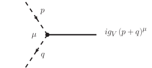
Figure 1: The Feynman rule for the $\rho\pi\pi$ vertex, where the solid line represents $\rho^{0}$’s on-shell state and dashed lines represent $\pi^{\pm}$’s on-shell states.

The self-energies corresponding to leading order (LO) Feynman diagrams in Fig. (2) are given as

$$\Sigma_{\mu\nu}^{<}(x,p) = -g_{V}^{2}\int\frac{d^{4}k_{1}}{(2\pi\hbar)^{4}}\int\frac{d^{4}k_{2}}{(2\pi\hbar)^{4}}(2\pi\hbar)^{4}\delta^{(4)}\left(p-k_{1}+k_{2}\right)$$ (20)

$$\times\left(k_{1\mu}+k_{2\mu}\right)\left(k_{1\nu}+k_{2\nu}\right)S^{<}(x,k_{1})S^{>}(x,k_{2}),$$

$$\Sigma_{\mu\nu}^{>}(x,p) = -g_{V}^{2}\int\frac{d^{4}k_{1}}{(2\pi\hbar)^{4}}\int\frac{d^{4}k_{2}}{(2\pi\hbar)^{4}}\left(2\pi\hbar\right)^{4}\delta^{(4)}\left(p-k_{1}+k_{2}\right)$$ (21)

$$\times\left(k_{1\mu}+k_{2\mu}\right)\left(k_{1\nu}+k_{2\nu}\right)S^{>}(x,k_{1})S^{<}(x,k_{2}).$$

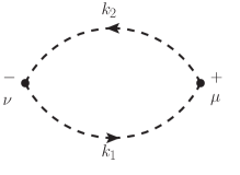
(a)

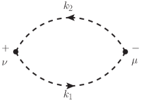
(b)

Figure 2: Leading-order Feynman diagrams for (a) $\Sigma_{\mu\nu}^{<}(x,p)$ and (b) $\Sigma_{\mu\nu}^{>}(x,p)$, where dashed lines represent propagators of $\pi^{\pm}$ mesons. The external moment $p$ is flowing from left to right.

In deriving Eq. (16), we have chosen $p^{0}>0$, so $k_{1}^{0}$ and $k_{2}^{0}$ must satisfy $k_{1}^{0}>0$ and $k_{2}^{0}<0$, which means the on-shell process $\rho^{0}\leftrightarrow\pi^{+}\pi^{-}$ is allowed but $\pi^{\pm}\leftrightarrow\rho^{0}\pi^{\pm}$ is forbidden. The discussion about the sign of $k_{1}^{0}$ and $k_{2}^{0}$ can be found in Ref. (Sheng:2022ffb, ).

Consequently, the LO self-energies in (20) and (21) can be put into the form

$$\Sigma_{\mu\nu}^{<}(x,p) = -g_{V}^{2}\int\frac{d^{3}k_{1}}{(2\pi\hbar)^{3}2E_{k_{1}}^{\pi}}\int\frac{d^{3}k_{2}}{(2\pi\hbar)^{3}2E_{k_{2}}^{\pi}}(2\pi\hbar)^{4}\delta^{(4)}\left(p-k_{1}-k_{2}\right)$$ (22)

$$\times\left(k_{1\mu}-k_{2\mu}\right)\left(k_{1\nu}-k_{2\nu}\right)f_{\pi^{+}}(x,\mathbf{k}_{1})f_{\pi^{-}}(x,\mathbf{k}_{2}),$$

$$\Sigma_{\mu\nu}^{>}(x,p) = -g_{V}^{2}\int\frac{d^{3}k_{1}}{(2\pi\hbar)^{3}2E_{k_{1}}^{\pi}}\int\frac{d^{3}k_{2}}{(2\pi\hbar)^{3}2E_{k_{2}}^{\pi}}(2\pi\hbar)^{4}\delta^{(4)}\left(p-k_{1}-k_{2}\right)$$ (23)

$$\times\left(k_{1\mu}-k_{2\mu}\right)\left(k_{1\nu}-k_{2\nu}\right)\left[1+f_{\pi^{+}}(x,\mathbf{k}_{1})\right]\left[1+f_{\pi^{-}}(x,\mathbf{k}_{2})\right].$$

Substituting above equations into Eq. (16), we obtain

$$C_{\mathrm{coal}/\mathrm{diss}}^{(0)}\left(\rho^{0}\leftrightarrow\pi^{+}\pi^{-}\right) = \frac{g_{V}^{2}}{E_{p}^{\rho}}\int\frac{d^{3}k}{(2\pi\hbar)^{3}4E_{k}^{\pi}E_{p-k}^{\pi}}2\pi\hbar\delta\left(E_{p}^{\rho}-E_{k}^{\pi}-E_{p-k}^{\pi}\right)$$ (24)

$$\times\left[\delta_{\lambda_{2}\lambda_{2}^{\prime}}k\cdot\epsilon^{*}(\lambda_{1},\mathbf{p})k\cdot\epsilon(\lambda_{1}^{\prime},\mathbf{p})+\delta_{\lambda_{1}\lambda_{1}^{\prime}}k\cdot\epsilon(\lambda_{2},\mathbf{p})k\cdot\epsilon^{*}(\lambda_{2}^{\prime},\mathbf{p})\right]$$

$$\times\left\{f_{\pi^{+}}(x,\mathbf{k})f_{\pi^{-}}(x,{\bf p}-\mathbf{k})\left[\delta_{\lambda_{1}^{\prime}\lambda_{2}^{\prime}}+f_{\lambda_{1}^{\prime}\lambda_{2}^{\prime}}(x,{\bf p})\right]\right.$$

$$\left.-\left[1+f_{\pi^{+}}(x,\mathbf{k})\right]\left[1+f_{\pi^{-}}(x,{\bf p}-\mathbf{k})\right]f_{\lambda_{1}^{\prime}\lambda_{2}^{\prime}}(x,{\bf p})\right\},$$

where we have used Eq. (7).

IV.2 Next-to-leading order

The Feynman diagrams for $\Sigma^{<}(x,p)$ at next-to-leading order (NLO) are shown in Fig. (3). Considering the difference between $\Sigma^{<}(x,p)$ and $\Sigma^{>}(x,p)$ is to interchange between the positive and negative branch, we can evaluate $\Sigma^{<}(x,p)$ first and then replace $\lessgtr$ with $\gtrless$ in $\Sigma^{<}(x,p)$ to obtain $\Sigma^{>}(x,p)$. The free pion’s Feynman propagators with time and reverse-time order are

$$S^{F}(k) = \frac{i}{k^{2}-m_{\pi}^{2}},$$ (25)

$$S^{\overline{F}}(k) = \frac{-i}{k^{2}-m_{\pi}^{2}}.$$ (26)

The medium corrections for $S^{F}$ and $S^{\overline{F}}$ will be discussed in the next subsection.

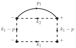
(a)

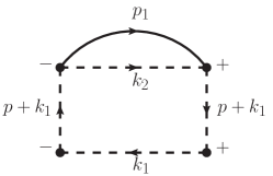
(b)

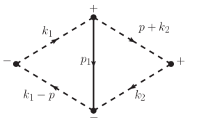
(c)

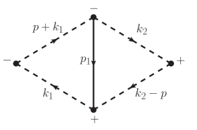
(d)

Figure 3: Feynman diagrams for $\Sigma_{\mu\nu}^{<}(x,p)$ at the next-to-leading order. The solid lines represent $\rho^{0}$ meson’s propagators and dashed lines represent the propagators of $\pi^{\pm}$ mesons. The external momentum $p$ is flowing from left to right.

We can see that Fig. (3)(a) and (b) are different in orientations of pion loops, and Fig. (3)(c) and (d) are different in time branches for two middle points with momentum $p_{1}$. In Fig. (3) we choose a particular direction for $p_{1}$ in the vector meson’s propagator, actually one is free to choose any direction without changing the final result. Other combinations of time branches for upper vertices in Fig. (3)(a) and (b) and middle vertices in Fig. (3)(c) and (d) correspond to loop corrections to propagators and vertices respectively, which need renormalization as in quantum field theory in vacuum. For example, in Fig. (3)(a), other combinations of time branches for two upper vertices (from left to right) are $++$ and $--$, which correspond to the loop correction to the right and left pion propagator respectively, as shown in Fig. 4. As another example, in Fig. (3)(c), other combinations of time branches for two upper vertices (from left to right) are $++$ and $--$, which correspond to the loop correction to the right and left vertex respectively, as shown in Fig. 4.

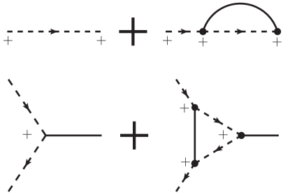
(a)

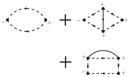
(b)

Figure 4: Examples of propagator and vertex corrections.

Now we can obtain collision terms at NLO. The result has three parts corresponding to three processes, $\rho^{0}\pi^{+}\leftrightarrow\rho^{0}\pi^{+}$, $\rho^{0}\pi^{-}\leftrightarrow\rho^{0}\pi^{-}$ and $\rho^{0}\rho^{0}\leftrightarrow\pi^{+}\pi^{-}$,

$$C_{\mathrm{scat}}\left(\rho^{0}\pi^{\pm}\leftrightarrow\rho^{0}\pi^{\pm}\right) = \frac{4g_{V}^{4}}{E_{p}^{\rho}}\int\frac{d^{3}k_{1}}{\left(2\pi\hbar\right)^{3}2E_{k_{1}}^{\pi}}\int\frac{d^{3}k_{2}}{\left(2\pi\hbar\right)^{3}2E_{k_{2}}^{\pi}}\int\frac{d^{3}p_{1}}{\left(2\pi\hbar\right)^{3}2E_{p_{1}}^{\rho}}$$ (27)

$$\times\left(2\pi\hbar\right)^{4}\delta^{(4)}\left(p+k_{2}-p_{1}-k_{1}\right)$$

$$\times\left[\delta_{\lambda_{2}\lambda_{2}^{\prime}}D_{(1)}(s_{1},\lambda_{1})D_{(1)}^{*}(s_{2},\lambda_{1}^{\prime})+\delta_{\lambda_{1}\lambda_{1}^{\prime}}D_{(1)}(s_{1},\lambda_{2}^{\prime})D_{(1)}^{*}(s_{2},\lambda_{2})\right]$$

$$\times\left[f_{s_{1}s_{2}}(x,\mathbf{p}_{1})f_{\pi^{\pm}}(x,\mathbf{k}_{1})\left(1+f_{\pi^{\pm}}(x,\mathbf{k}_{2})\right)\left(\delta_{\lambda_{1}^{\prime}\lambda_{2}^{\prime}}+f_{\lambda_{1}^{\prime}\lambda_{2}^{\prime}}(x,{\bf p})\right)\right.$$

$$\left.-\left(\delta_{s_{1}s_{2}}+f_{s_{1}s_{2}}(x,\mathbf{p}_{1})\right)\left(1+f_{\pi^{\pm}}(x,\mathbf{k}_{1})\right)f_{\pi^{\pm}}(x,\mathbf{k}_{2})f_{\lambda_{1}^{\prime}\lambda_{2}^{\prime}}(x,{\bf p})\right],$$

$$C_{\mathrm{coal}/\mathrm{diss}}^{(1)}\left(\rho^{0}\rho^{0}\leftrightarrow\pi^{+}\pi^{-}\right) = \frac{4g_{V}^{4}}{E_{p}^{\rho}}\int\frac{d^{3}k_{1}}{\left(2\pi\hbar\right)^{3}2E_{k_{1}}^{\pi}}\int\frac{d^{3}k_{2}}{\left(2\pi\hbar\right)^{3}2E_{k_{2}}^{\pi}}\int\frac{d^{3}p_{1}}{\left(2\pi\hbar\right)^{3}2E_{p_{1}}^{\rho}}$$ (28)

$$\times\left(2\pi\hbar\right)^{4}\delta^{(4)}\left(p+p_{1}-k_{1}-k_{2}\right)$$

$$\times\left[\delta_{\lambda_{2}\lambda_{2}^{\prime}}D_{(2)}(s_{1},\lambda_{1}^{\prime})D_{(2)}^{*}(s_{2},\lambda_{1})+\delta_{\lambda_{1}\lambda_{1}^{\prime}}D_{(2)}(s_{1},\lambda_{2})D_{(2)}^{*}(s_{2},\lambda_{2}^{\prime})\right]$$

$$\times\left[f_{\pi^{+}}(x,\mathbf{k}_{1})f_{\pi^{-}}(x,\mathbf{k}_{2})\left(\delta_{s_{1}s_{2}}+f_{s_{1}s_{2}}(x,\mathbf{p}_{1})\right)\left(\delta_{\lambda_{1}^{\prime}\lambda_{2}^{\prime}}+f_{\lambda_{1}^{\prime}\lambda_{2}^{\prime}}(x,{\bf p})\right)\right.$$

$$\left.-\left(1+f_{\pi^{+}}(x,\mathbf{k}_{1})\right)\left(1+f_{\pi^{-}}(x,\mathbf{k}_{2})\right)f_{s_{1}s_{2}}(x,\mathbf{p}_{1})f_{\lambda_{1}^{\prime}\lambda_{2}^{\prime}}(x,{\bf p})\right],$$

where we have used $s_{1}$ and $s_{2}$ to label spin states in propagators of $\rho^{0}$, used Eq. (7) and the on-shell condition, and defined

$$D_{(1)}(s,\lambda)= \frac{\left[k_{1}\cdot\epsilon\left(s,\mathbf{p}_{1}\right)\right]\left[k_{2}\cdot\epsilon^{*}\left(\lambda,{\bf p}\right)\right]}{\left(p+k_{2}\right)^{2}-m_{\pi}^{2}}+\frac{\left[k_{2}\cdot\epsilon\left(s,\mathbf{p}_{1}\right)\right]\left[k_{1}\cdot\epsilon^{*}\left(\lambda,{\bf p}\right)\right]}{\left(p-k_{1}\right)^{2}-m_{\pi}^{2}},$$

$$D_{(2)}(s,\lambda)= \frac{\left[k_{1}\cdot\epsilon\left(s,\mathbf{p}_{1}\right)\right]\left[k_{2}\cdot\epsilon\left(\lambda,{\bf p}\right)\right]}{\left(p-k_{2}\right)^{2}-m_{\pi}^{2}}+\frac{\left[k_{2}\cdot\epsilon\left(s,\mathbf{p}_{1}\right)\right]\left[k_{1}\cdot\epsilon\left(\lambda,{\bf p}\right)\right]}{\left(p-k_{1}\right)^{2}-m_{\pi}^{2}}.$$ (29)

One can check that the collision terms are Hermitian in consistence with $f_{\lambda_{1}\lambda_{2}}$.

So far we have completed the derivation of the spin Boltzmann equation with collision terms at LO and NLO.

IV.3 Regulation of pion propagators

In the collision term $C_{\mathrm{scat}}\left(\rho^{0}\pi^{\pm}\leftrightarrow\rho^{0}\pi^{\pm}\right)$, there are pion propagators which may diverge at the pion mass pole. To regulate these pion propagators, we introduce self-energy corrections with medium effects as

$$S^{F}(k) = \frac{i}{k^{2}-m_{\pi}^{2}-\Sigma^{F}(k)}$$ (30)

$$S^{\overline{F}}(k) = \frac{-i}{k^{2}-m_{\pi}^{2}+\Sigma^{\overline{F}}(k)},$$ (31)

where $\Sigma^{F}$ is the self-energy for pions. The real part of the self-energy gives the mass correction, while the imaginary part is associated with the medium effect. In this work, we only consider the imaginary part of the self-energy since the mass correction from the real part is much smaller.

The Feynman diagram for the pion self-energy $\Sigma^{F}$ at LO is shown in Fig.(5) which is given by

$$-i\Sigma^{F}(k) = -g_{V}^{2}\int\frac{d^{4}k_{1}}{\left(2\pi\hbar\right)^{4}}S^{F}(k_{1})G_{\alpha\beta}^{F}(k-k_{1})\left(k+k_{1}\right)^{\alpha}\left(k+k_{1}\right)^{\beta}.$$ (32)

where the Feynman propagators in medium read

$$S^{F}(k) = \frac{i}{k^{2}-m_{\pi}^{2}+i\epsilon}+2\pi\hbar\delta\left(k^{2}-m_{\pi}^{2}\right)\left[\theta(k^{0})f_{\pi^{+}}(\mathbf{k})+\theta(-k^{0})f_{\pi^{-}}(-\mathbf{k})\right],$$ (33)

$$G_{\alpha\beta}^{F}(p) = -\frac{i\left(g_{\alpha\beta}-p_{\alpha}p_{\beta}/m_{\rho}^{2}\right)}{p^{2}-m_{\rho}^{2}+i\epsilon}+\left(2\pi\hbar\right)\delta\left(p^{2}-m_{\rho}^{2}\right)$$ (34)

$$\times\left[\theta(p^{0})\epsilon_{\alpha}\left(s_{1},{\bf p}\right)\epsilon_{\beta}^{*}\left(s_{2},{\bf p}\right)f_{s_{1}s_{2}}(\mathbf{p})+\theta(-p^{0})\epsilon_{\alpha}^{\ast}\left(s_{1},-{\bf p}\right)\epsilon_{\beta}\left(s_{2},-{\bf p}\right)f_{s_{2}s_{1}}(-\mathbf{p})\right],$$

which can be derived by substituting Eqs. (3) and (4) into Eqs. (8) and (9).

Figure 5: The Feynman diagram for pion self-energy $\Sigma^{F}$ at LO. The solid line represents the $\rho^{0}$ propagator and the dashed line represents the pion propagator.

Substituting Eqs. (33), (34) into Eq. (32), we obtain the imaginary part of the self-energy

$$\Gamma(k) \equiv \mathrm{Im}\Sigma^{F}(k)=2g_{V}^{2}\theta(k^{0})\int\frac{d^{3}k_{1}}{(2\pi\hbar)^{3}2E_{k_{1}}^{\pi}}\int\frac{d^{3}p}{(2\pi\hbar)^{3}2E_{p}^{\rho}}$$ (35)

$$\times(2\pi\hbar)^{4}\delta^{(4)}\left(k+k_{1}-p\right)f_{\pi^{-}}(\mathbf{k}_{1})\left[m_{\pi}^{2}-\frac{\left(k_{1}\cdot p\right)^{2}}{m_{\rho}^{2}}\right]$$

$$+2g_{V}^{2}\theta(-k^{0})\int\frac{d^{3}k_{1}}{(2\pi\hbar)^{3}2E_{k_{1}}^{\pi}}\int\frac{d^{3}p}{(2\pi\hbar)^{3}2E_{p}^{\rho}}$$

$$\times(2\pi\hbar)^{4}\delta^{(4)}\left(k-k_{1}+p\right)f_{\pi^{+}}(\mathbf{k}_{1})\left[m_{\pi}^{2}-\frac{\left(k_{1}\cdot p\right)^{2}}{m_{\rho}^{2}}\right],$$

where we have assumed that $k$ is near the mass-shell, since the self-energy’s correction to $k^{2}-m_{\pi}^{2}$ in Eq. (30) is negligible if $k$ is far off-shell. Under such an assumption, processes such as $\pi^{+}\rightarrow\pi^{+}\rho^{0}$ are forbidden, so the self-energy can be simplified. With the imaginary part of the self-energy in (35), the function $D_{(1)}(s,\lambda)$ in $C_{\mathrm{scat}}\left(\rho^{0}\pi^{\pm}\leftrightarrow\rho^{0}\pi^{\pm}\right)$ in Eq. (29) becomes

$$D_{\pi^{+}(1)}(s,\lambda)= \frac{\left[k_{1}\cdot\epsilon\left(s,\mathbf{p}_{1}\right)\right]\left[k_{2}\cdot\epsilon^{*}\left(\lambda,{\bf p}\right)\right]}{\left(p+k_{2}\right)^{2}-m_{\pi}^{2}+i\Gamma(p+k_{2})}+\frac{\left[k_{2}\cdot\epsilon\left(s,\mathbf{p}_{1}\right)\right]\left[k_{1}\cdot\epsilon^{*}\left(\lambda,{\bf p}\right)\right]}{\left(p-k_{1}\right)^{2}-m_{\pi}^{2}+i\Gamma(-p+k_{1})},$$

$$D_{\pi^{-}(1)}(s,\lambda)= \frac{\left[k_{1}\cdot\epsilon\left(s,\mathbf{p}_{1}\right)\right]\left[k_{2}\cdot\epsilon^{*}\left(\lambda,{\bf p}\right)\right]}{\left(p+k_{2}\right)^{2}-m_{\pi}^{2}+i\Gamma(-p-k_{2})}+\frac{\left[k_{2}\cdot\epsilon\left(s,\mathbf{p}_{1}\right)\right]\left[k_{1}\cdot\epsilon^{*}\left(\lambda,{\bf p}\right)\right]}{\left(p-k_{1}\right)^{2}-m_{\pi}^{2}+i\Gamma(p-k_{1})}.$$ (36)

which are different for $\rho^{0}\pi^{+}\leftrightarrow\rho^{0}\pi^{+}$ and $\rho^{0}\pi^{-}\leftrightarrow\rho^{0}\pi^{-}$ processes.

V Numerical results

V.1 Initial condition without elliptic flow

Since we are studying the spin alignment of $\rho^{0}$ in a pion gas, we assume the pion density is much larger than the density of $\rho^{0}$, $f_{\lambda_{1}\lambda_{2}}\ll f_{\pi^{\pm}}$, so the influence of $\rho^{0}$ mesons on pions is negligible. We further assume that $\pi^{\pm}$ are in global thermal equilibrium, so they obey the Bose-Einstein distribution

$$f_{\pi^{\pm}}(x,\mathbf{p})=f_{\pi^{\pm}}(\mathbf{p})=\frac{1}{\exp\left[\beta\left(E_{p}\mp\mu_{\pi}\right)\right]-1},$$ (37)

where $\beta=1/T$ is the inverse temperature, $\mu_{\pi}$ is the chemical potential for $\pi^{+}$. Here we neglected the spatial dependence of distributions. We choose $\mu_{\pi}$=0, and $T=156.5$ MeV corresponding to the chemical freezeout temperature. Because $f_{\lambda_{1}\lambda_{2}}\ll f_{\pi^{\pm}}$ we can neglect the terms of order $f_{\lambda_{1}\lambda_{2}}^{2}$ relative to $f_{\lambda_{1}\lambda_{2}}$. Since the temperature is much less than $m_{\rho}$, the contribution from the process $\rho^{0}\rho^{0}\leftrightarrow\pi^{+}\pi^{-}$ is negligible (two orders of magnitude smaller) relative to $C_{\mathrm{coal}/\mathrm{diss}}^{(0)}\left(\rho^{0}\leftrightarrow\pi^{+}\pi^{-}\right)$.

In summary, the collision terms that we take into account are $C_{\mathrm{coal}/\mathrm{diss}}^{(0)}\left(\rho^{0}\leftrightarrow\pi^{+}\pi^{-}\right)$ and $C_{\mathrm{scat}}\left(\rho^{0}\pi^{\pm}\leftrightarrow\rho^{0}\pi^{\pm}\right)$. For $f_{\pi^{+}}=f_{\pi^{-}}$, we can simply have $C_{\mathrm{scat}}\left(\rho^{0}\pi^{+}\leftrightarrow\rho^{0}\pi^{+}\right)=C_{\mathrm{scat}}\left(\rho^{0}\pi^{-}\leftrightarrow\rho^{0}\pi^{-}\right)$.

Considering the spin Boltzmann equation (18) is an integral-differential equation, we use Monte Carlo method to solve it. We build a 50$\times$50$\times$50 lattice in momentum space for $\rho^{0}$ with lattice cell size 100$\times$100$\times$100 MeV³, so the range $p_{x}$, $p_{y}$ and $p_{z}$ is $\left[-2.5,2.5\right]$ GeV, which is big enough compared with the temperature. The value of $\rho_{00}=f_{00}/\mathrm{Tr}(f)$ represents the spin alignment of $\rho^{0}$ mesons.

In the first case, we consider the initial condition without neutral rho mesons, i.e. $f_{\lambda_{1}\lambda_{2}}(t=0)=0$. The time step for simulation is chosen to be $5\times 10^{-6}$ MeV^-1$\approx 10^{-3}$ fm/c. The spin alignments of rho mesons as functions of $p_{T}$ in the pseudorapidity range $|\eta|<1$ at different time are shown in Fig. (6). The spin alignments ($p_{T}$ integrated) in different pseudorapidity ranges are shown in Fig. (7). The precision of $\rho_{00}$ is about $10^{-3}$ in Monte Carlo method, so the results less than $10^{-3}$ are not reliable. However, we can still see the time and pseudorapidity dependence of the spin alignment from these results.

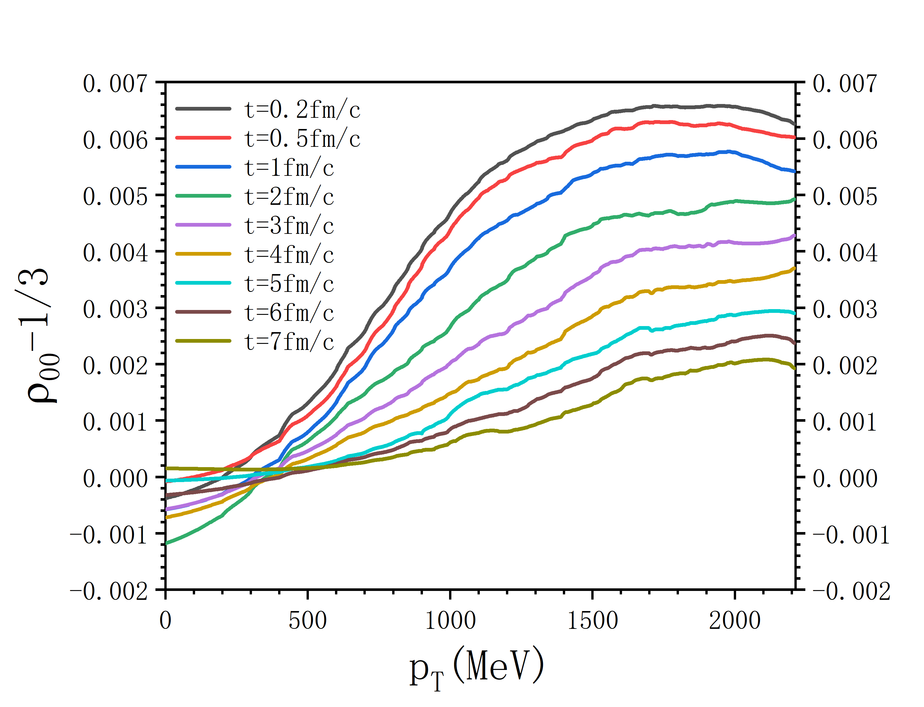
Figure 6: The spin alignment as functions of $p_{T}$ at different time. The initial distribution of rho mesons is set to $f_{\lambda_{1}\lambda_{2}}(t=0)=0$.

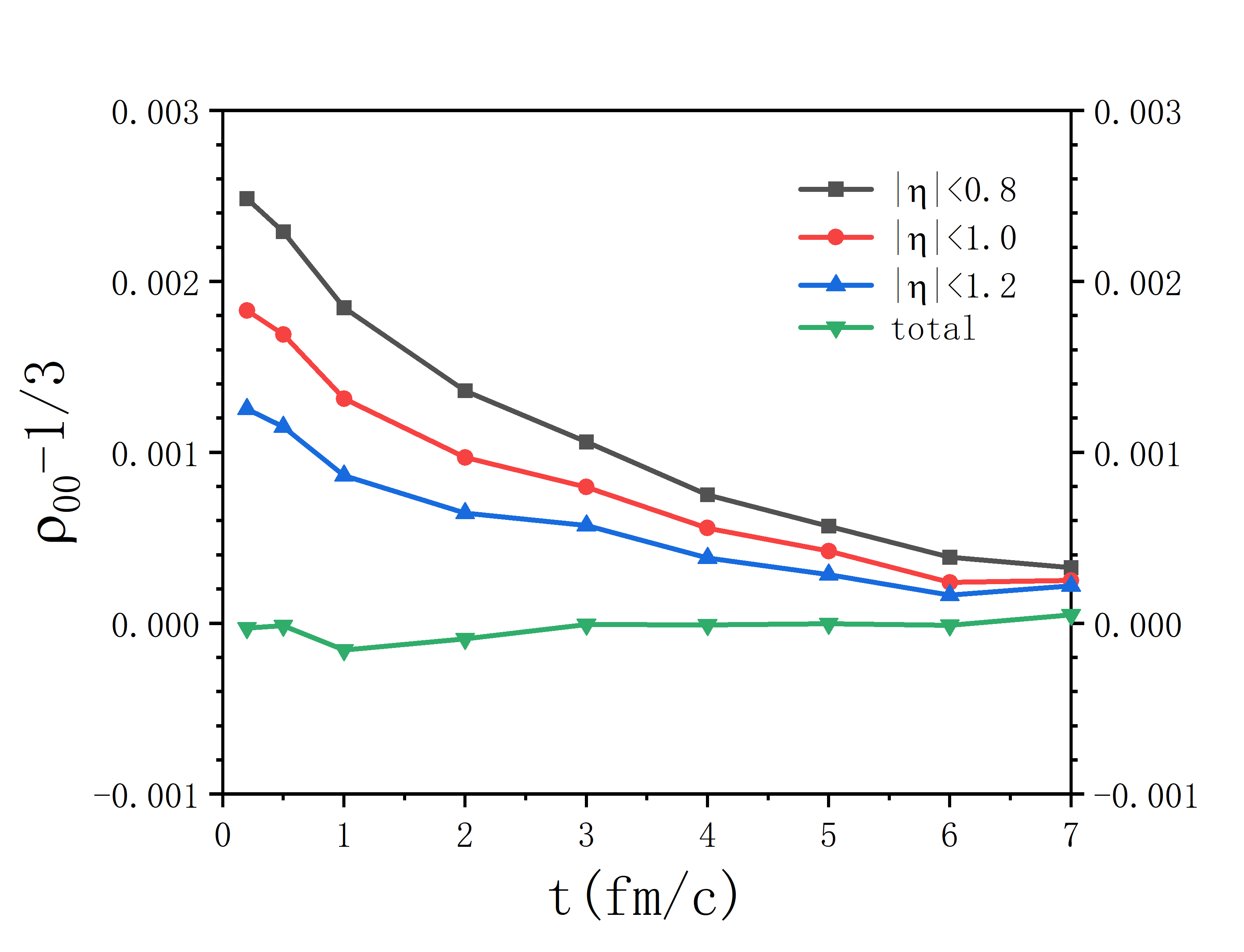
Figure 7: The $p_{T}$-integrated spin alignment in different pseudorapidity ranges for the initial distribution $f_{\lambda_{1}\lambda_{2}}(t=0)=0$.

We notice that $\rho_{00}$ is slightly larger than 1/3 in the central rapidity region of rho mesons though the pion distribution is isotropic. It is because that we choose $+y$ to be the spin quantization direction, which is different from $x$ and $z$. More specifically, the produced rho mesons with momenta in $\pm y$ direction have $\rho_{00}>1/3$, while those with momenta near the $xz$ plane have $\rho_{00}<1/3$. The spin alignment in the whole momentum space must be zero because of the isotropic pion distribution and angular momentum conservation, as shown by the green line in Fig. (7). Therefore if we exclude rho mesons with momenta near $\pm z$ direction, i.e. the forward and backward rapidity region, we have $\rho_{00}>1/3$. The larger central pseudorapidity range we choose, the smaller spin alignment we obtain. Since the scattering term contributes significantly to a thermalization effect, we notice that the spin alignment decreases rapidly with time.

In the second case, we consider a more realistic initial condition by assuming an initial value of the spin alignment at the hadronization time when the rho meson is formed by recombination of quarks. We set the initial distribution of the rho meson as a thermal distribution with the spin alignment $\rho_{00}=0.4$ (larger than 1/3), then the matrix valued spin distribution is put into the form

$$f_{\lambda_{1}\lambda_{2}} = \mathrm{diag}(0.9,1.2,0.9)\times f_{\mathrm{BE}},$$ (38)

where $f_{\mathrm{BE}}$ is the Bose-Einstein distribution for the rho meson with zero chemical potential. The time step for simulation is chosen to be $5\times 10^{-5}$ MeV${}^{-1}\approx$0.01 fm/c. In the pseudorapidity range $|\eta|<1$, the numerical results for the spin alignment as functions of $p_{T}$ at different time are shown in Fig. (8). The results for the $p_{T}$-integrated spin alignment in different pseudorapidity ranges are shown in Fig. (9). We can see that the spin alignment is almost independent of the pseudorapidity range, because it is mostly contributed from initial rho mesons with non-vanishing spin alignment instead of from newly generated rho mesons. More importantly, we see that $\rho_{00}-1/3$ decreases rapidly from the initial value 0.066 to 0.006 at $t=4$ fm/c, meaning that the initial value of the spin alignment can be easily washed out by the interaction between rho mesons and pions.

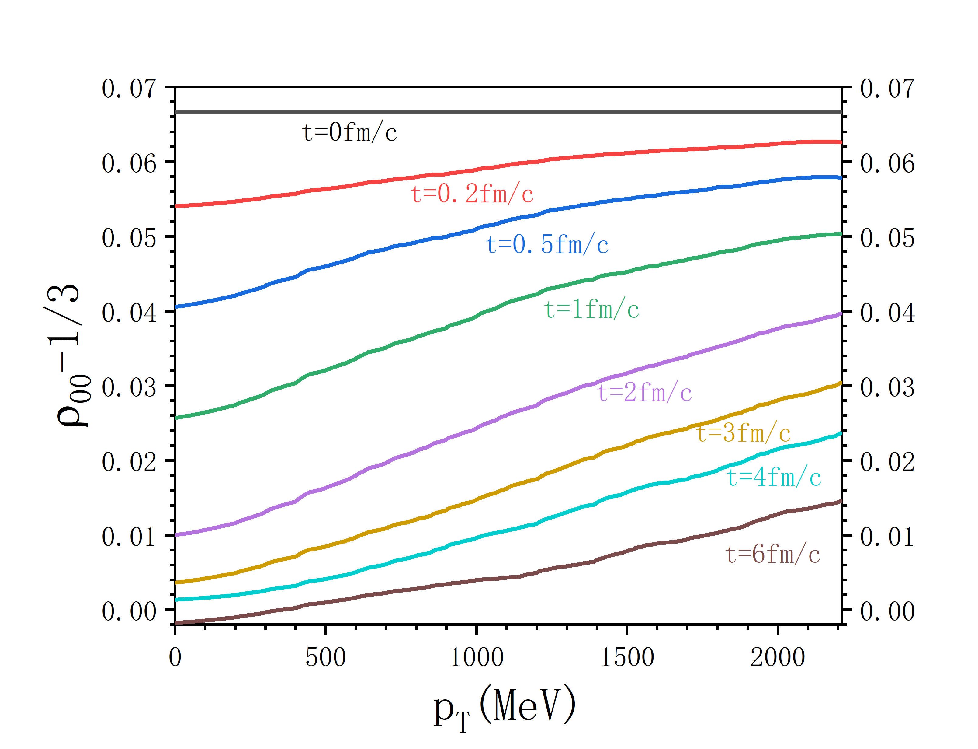
Figure 8: The spin alignment as functions of $p_{T}$ in $|\eta|<1$ at different time with the initial distribution (38) that corresponds to $\rho_{00}=0.4>1/3$.

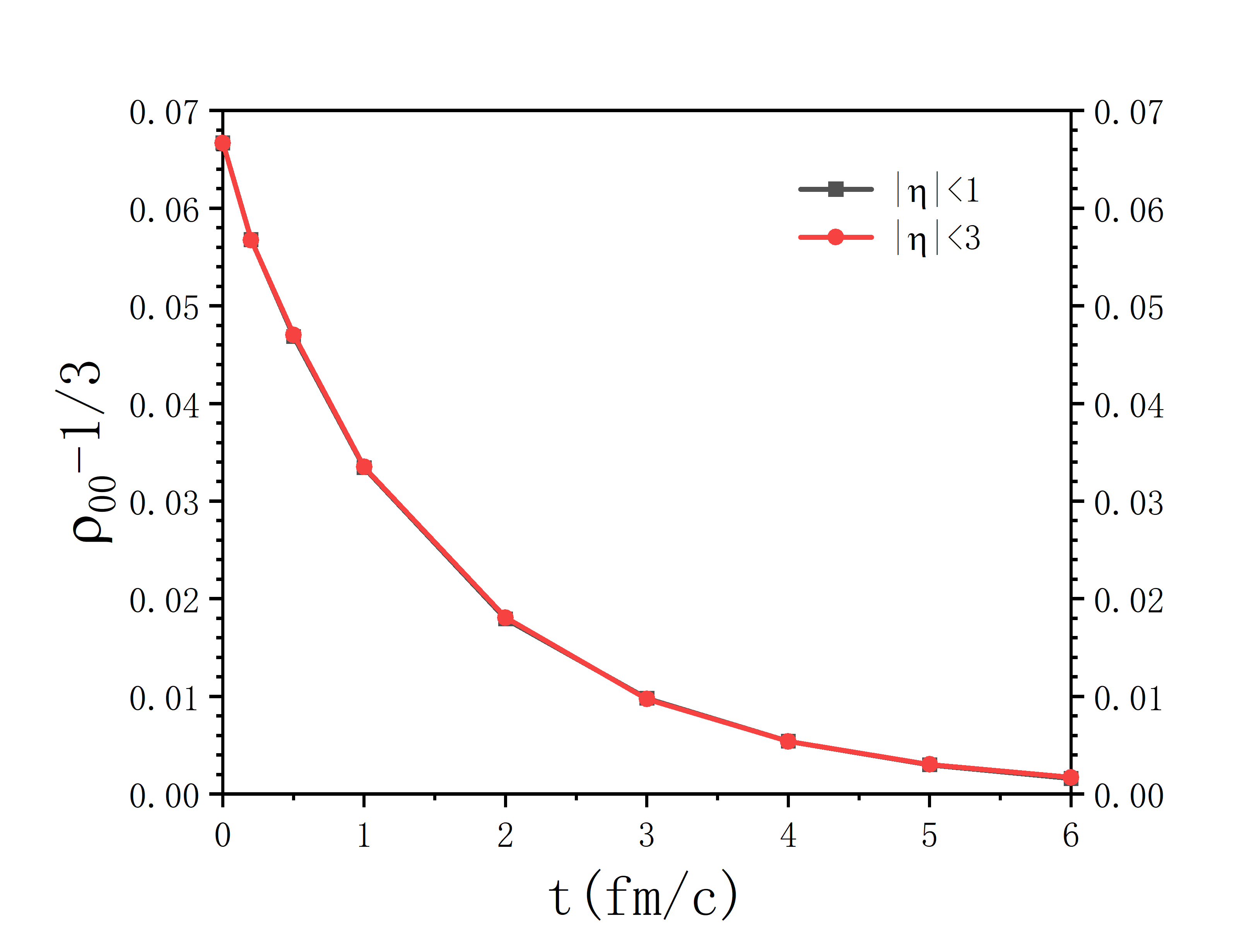
Figure 9: The $p_{T}$-integrated spin alignment in different pseudorapidity ranges with the initial distribution (38).

We can also consider $\rho_{00}=0.27$ (less than 1/3) at the initial time. Then the matrix valued spin distribution is set to

$$f_{\lambda_{1}\lambda_{2}} = \mathrm{diag}(1.1,0.8,1.1)\times f_{\mathrm{BE}}.$$ (39)

The results are shown in Figs. (10) and (11). We see that the spin alignment relaxes to 1/3 rapidly.

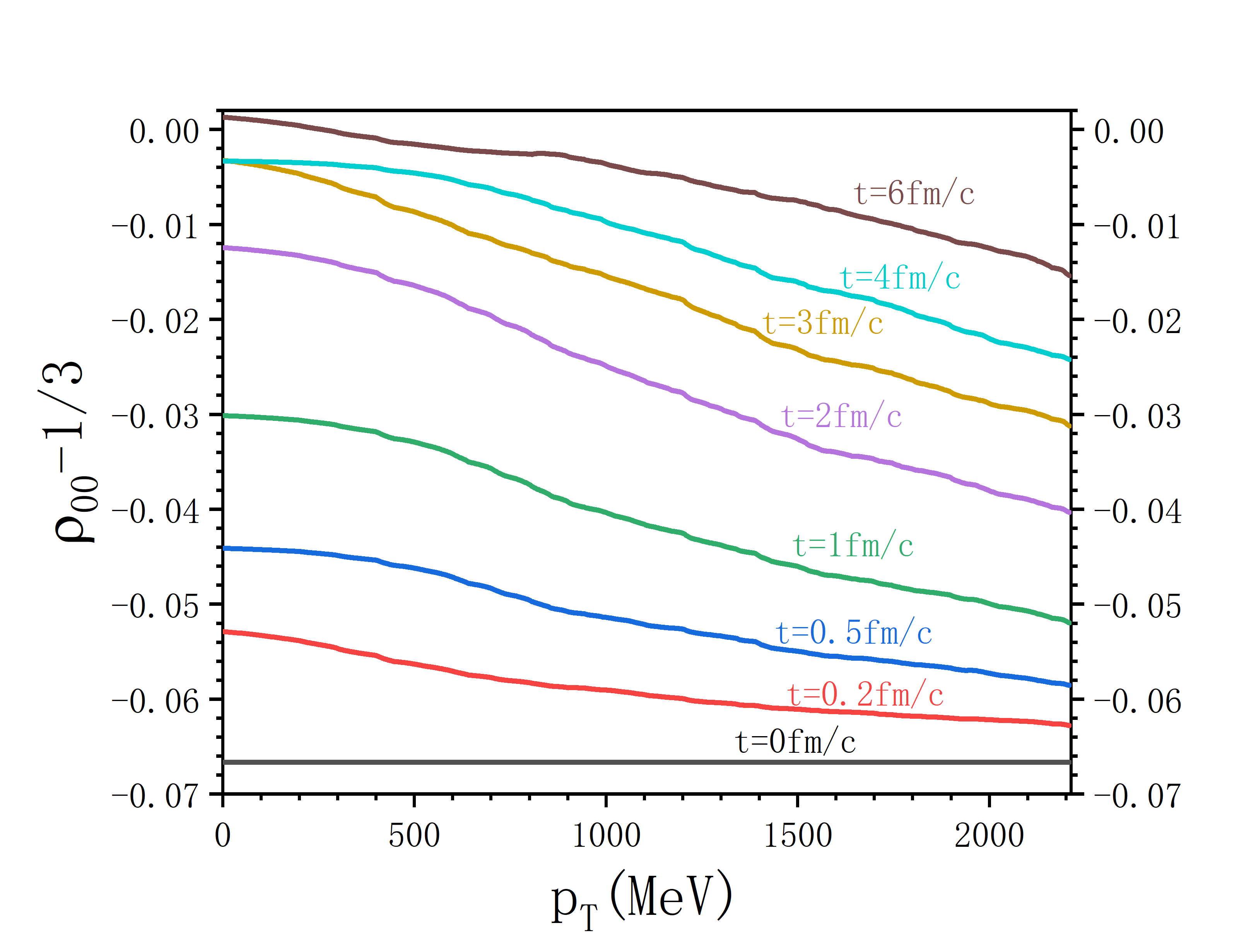
Figure 10: The spin alignment as functions of $p_{T}$ at different time with the initial distribution (39) that corresponds to $\rho_{00}=0.27<1/3$.

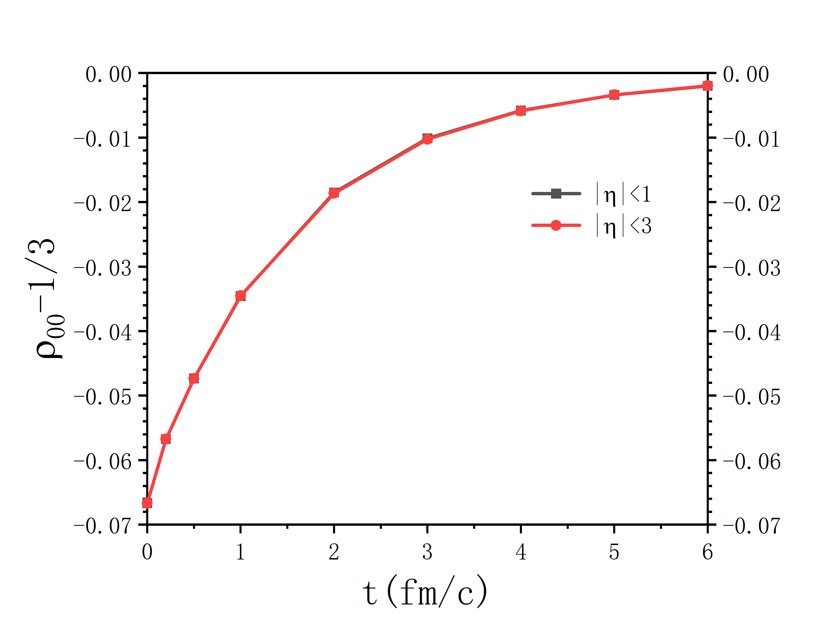
Figure 11: The $p_{T}$-integrated spin alignment in different pseudorapidity ranges with the initial distribution (39).

V.2 Initial condition with elliptic flow

In order to see the $v_{2}$ influence on the spin alignment of $\rho^{0}$, we use the blast wave model (Bondorf:1978kz, ; Siemens:1978pb, ; Schnedermann:1993ws, ; Retiere:2003kf, ) to describe the space-time evolution of the fireball in heavy-ion collisions. The idea is as follows. We assume Eq. (19) describes the time evolution of $f_{\lambda_{1}\lambda_{2}}(x,\mathbf{p})$ in the fluid element’s comoving frame located at $x$. The fluid four-velocity $u^{\mu}(x)$ is described by the blast wave model for the boost invariant expansion of the fireball along $z$ direction. The emission function of the blast wave model has the form (Retiere:2003kf, )

$$S(r,\phi_{s},p) = \theta(R-r)F(u,p),$$ (40)

where $R$ is the fireball’s radius, $r$ and $\phi_{s}$ are the radial position and the azimutal angle inside the fireball, $p$ is the particle’s momentum, $F(u,p)$ is some kind of the momentum distribution function depending on the fluid velocity that can be parameterized as

$$u^{\mu}(r,\phi_{s})=\left(\cosh\rho(r,\phi_{s}),\sinh\rho(r,\phi_{s})\cos\phi_{s},\sinh\rho(r,\phi_{s})\sin\phi_{s},0\right),$$ (41)

where the radial flow rapidity $\rho$ is given by

$$\rho(r,\phi_{s}) = \frac{r}{R}\left[\rho_{0}+\rho_{2}\cos(2\phi_{s})\right].$$ (42)

Here $\rho_{0}$ and $\rho_{2}$ are two parameters, and $\rho_{2}$ gives the elliptic flow. Note that without loss of generality we have set space-time rapidity zero in $u^{\mu}(r,\phi_{s})$ corresponding to $z=0$.

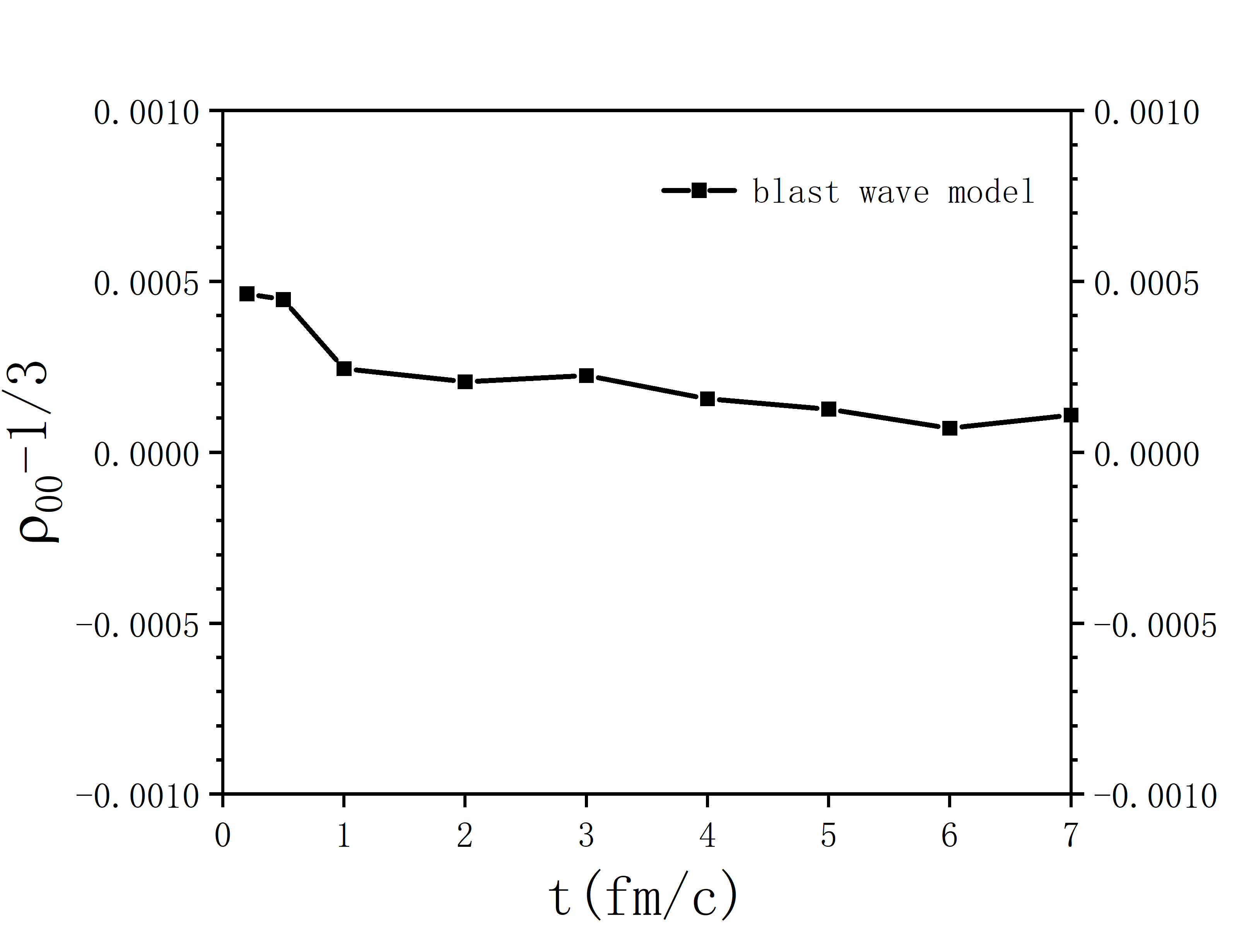
Figure 12: The spin alignment of the neutral rho meson at $z=0$ for $|\eta|<1$ in the blast wave model with the elliptic flow.

The parameters are chosen as $R=13$ fm, $\rho_{0}=0.89$, $\rho_{2}=0.06$ (Retiere:2003kf, ). We assume $f_{\lambda_{1}\lambda_{2}}=0$ at the initial time. Then with Eq. (40) and these parameters we can calculate the spin alignment at $z=0$ as follows

$$\rho_{00} = \frac{\int_{|\eta|<1}d^{3}p\int_{0}^{R}rdrd\phi_{s}f_{00}(u,p)}{\int_{|\eta|<1}d^{3}p\int_{0}^{R}rdrd\phi_{s}\mathrm{tr}f(u,p)},$$ (43)

where we set $F(u,p)$ to $f_{\lambda_{1}\lambda_{2}}(u,p)$. It is obvious that $\rho_{00}$ in Eq. (43) encodes the effect of the elliptic flow. The results for $\rho_{00}$ are shown in Fig. 12 indicating that its deviation from 1/3 is positive but in the order of $10^{-4}$.

VI Conclusions and discussions

Using two-point Green’s functions and Kadanoff-Baym equation in the closed-time path formalism for vector mesons developed in the previous work (Sheng:2022ffb, ), we derived spin kinetic or Boltzmann equations for neutral rho mesons in a pion gas. The $\rho\pi\pi$ coupling is described by the chiral effective theory. The collision terms in the pion gas at the leading and next-to-leading order are obtained. We simulated the evolution of the matrix valued spin distribution (spin density matrix) of neutral rho mesons by the Monte Carlo method. In the simulation, we have assumed the Bose-Einstein distribution for pions with $T=156.5$ MeV and vanishing chemical potential. The numerical results show that the interaction of pions and neutral rho mesons creates very small spin alignment for rho mesons in the central rapidity region if there is no rho meson in the system at the initial time. But there is no spin alignment in the full rapidity range since pions’ momenta are isotropic. Such a small spin alignment in the central rapidity region will decay rapidly toward zero in later time. If there are rho mesons with a sizable spin alignment at the initial time the spin alignment will also decrease rapidly. We also considered the effect on $\rho_{00}$ from the elliptic flow of pions in the blast wave model. With vanishing spin alignment at the initial time, the deviation of $\rho_{00}$ from 1/3 is positive but very small.

The work can be improved or extended by loosening some approximations or restrictions. For example, we can consider fluctuations in the temperature and the distribution of pions in collision terms, or we can consider other vector mesons in a hadrons gas. These can be done in the future.

- (1) S. J. Barnett, Rev. Mod. Phys. 7, 129 (1935).
- (2) A. Einstein and W. de Haas, Deutsche Physikalische Gesellschaft, Verhandlungen 17, 152 (1915).
- (3) Z.-T. Liang and X.-N. Wang, Phys. Rev. Lett. 94, 102301 (2005), nucl-th/0410079, [Erratum: Phys.Rev.Lett. 96, 039901 (2006)].
- (4) Z.-T. Liang and X.-N. Wang, Phys. Lett. B 629, 20 (2005), nucl-th/0411101.
- (5) B. Betz, M. Gyulassy, and G. Torrieri, Phys. Rev. C 76, 044901 (2007), 0708.0035.
- (6) J.-H. Gao et al., Phys. Rev. C 77, 044902 (2008), 0710.2943.
- (7) F. Becattini, F. Piccinini, and J. Rizzo, Phys. Rev. C 77, 024906 (2008), 0711.1253.
- (8) G. Bunce et al., Phys. Rev. Lett. 36, 1113 (1976).
- (9) STAR, L. Adamczyk et al., Nature 548, 62 (2017), 1701.06657.
- (10) STAR, J. Adam et al., Phys. Rev. C 98, 014910 (2018), 1805.04400.
- (11) HADES, R. Abou Yassine et al., Phys. Lett. B 835, 137506 (2022), 2207.05160.
- (12) ALICE, S. Acharya et al., Phys. Rev. Lett. 128, 172005 (2022), 2107.11183.
- (13) STAR, J. Adam et al., Phys. Rev. Lett. 126, 162301 (2021), 2012.13601.
- (14) I. Karpenko and F. Becattini, Eur. Phys. J. C 77, 213 (2017), 1610.04717.
- (15) H. Li, L.-G. Pang, Q. Wang, and X.-L. Xia, Phys. Rev. C 96, 054908 (2017), 1704.01507.
- (16) Y. Xie, D. Wang, and L. P. Csernai, Phys. Rev. C 95, 031901 (2017), 1703.03770.
- (17) Y. Sun and C. M. Ko, Phys. Rev. C 96, 024906 (2017), 1706.09467.
- (18) M. Baznat, K. Gudima, A. Sorin, and O. Teryaev, Phys. Rev. C 97, 041902 (2018), 1701.00923.
- (19) S. Shi, K. Li, and J. Liao, Phys. Lett. B 788, 409 (2019), 1712.00878.
- (20) X.-L. Xia, H. Li, Z.-B. Tang, and Q. Wang, Phys. Rev. C 98, 024905 (2018), 1803.00867.
- (21) D.-X. Wei, W.-T. Deng, and X.-G. Huang, Phys. Rev. C 99, 014905 (2019), 1810.00151.
- (22) B. Fu, K. Xu, X.-G. Huang, and H. Song, Phys. Rev. C 103, 024903 (2021), 2011.03740.
- (23) S. Ryu, V. Jupic, and C. Shen, Phys. Rev. C 104, 054908 (2021), 2106.08125.
- (24) B. Fu, S. Y. F. Liu, L. Pang, H. Song, and Y. Yin, Phys. Rev. Lett. 127, 142301 (2021), 2103.10403.
- (25) X.-G. Deng, X.-G. Huang, and Y.-G. Ma, (2021), 2109.09956.
- (26) F. Becattini, M. Buzzegoli, G. Inghirami, I. Karpenko, and A. Palermo, Phys. Rev. Lett. 127, 272302 (2021), 2103.14621.
- (27) X.-Y. Wu, C. Yi, G.-Y. Qin, and S. Pu, Phys. Rev. C 105, 064909 (2022), 2204.02218.
- (28) Q. Wang, Nucl. Phys. A 967, 225 (2017), 1704.04022.
- (29) W. Florkowski, A. Kumar, and R. Ryblewski, Prog. Part. Nucl. Phys. 108, 103709 (2019), 1811.04409.
- (30) J.-H. Gao, Z.-T. Liang, Q. Wang, and X.-N. Wang, Lect. Notes Phys. 987, 195 (2021), 2009.04803.
- (31) X.-G. Huang, J. Liao, Q. Wang, and X.-L. Xia, (2020), 2010.08937.
- (32) J.-H. Gao, G.-L. Ma, S. Pu, and Q. Wang, Nucl. Sci. Tech. 31, 90 (2020), 2005.10432.
- (33) F. Becattini and M. A. Lisa, Ann. Rev. Nucl. Part. Sci. 70, 395 (2020), 2003.03640.
- (34) F. Becattini, Rept. Prog. Phys. 85, 122301 (2022), 2204.01144.
- (35) K. Schilling, P. Seyboth, and G. E. Wolf, Nucl. Phys. B 15, 397 (1970), [Erratum: Nucl.Phys.B 18, 332 (1970)].
- (36) Y.-G. Yang, R.-H. Fang, Q. Wang, and X.-N. Wang, Phys. Rev. C 97, 034917 (2018), 1711.06008.
- (37) A. H. Tang et al., Phys. Rev. C 98, 044907 (2018), 1803.05777, [Erratum: Phys.Rev.C 107, 039901 (2023)].
- (38) STAR, M. S. Abdallah et al., Nature 614, 244 (2023), 2204.02302.
- (39) X.-L. Xia, H. Li, X.-G. Huang, and H. Zhong Huang, Phys. Lett. B 817, 136325 (2021), 2010.01474.
- (40) J.-H. Gao, Phys. Rev. D 104, 076016 (2021), 2105.08293.
- (41) B. Müller, B. Müller, D.-L. Yang, and D.-L. Yang, Phys. Rev. D 105, L011901 (2022), 2110.15630, [Erratum: Phys.Rev.D 106, 039904 (2022)].
- (42) F. Li and S. Y. F. Liu, (2022), 2206.11890.
- (43) D. Wagner, N. Weickgenannt, and E. Speranza, Phys. Rev. Res. 5, 013187 (2023), 2207.01111.
- (44) A. Kumar, B. Müller, and D.-L. Yang, Phys. Rev. D 107, 076025 (2023), 2212.13354.
- (45) W.-B. Dong, Y.-L. Yin, X.-L. Sheng, S.-Z. Yang, and Q. Wang, (2023), 2311.18400.
- (46) A. Kumar, B. Müller, and D.-L. Yang, Phys. Rev. D 108, 016020 (2023), 2304.04181.
- (47) J.-H. Gao and S.-Z. Yang, (2023), 2308.16616.
- (48) X.-L. Sheng, L. Oliva, and Q. Wang, Phys. Rev. D 101, 096005 (2020), 1910.13684, [Erratum: Phys.Rev.D 105, 099903 (2022)].
- (49) X.-L. Sheng, L. Oliva, Z.-T. Liang, Q. Wang, and X.-N. Wang, (2022), 2206.05868.
- (50) X.-L. Sheng, L. Oliva, Z.-T. Liang, Q. Wang, and X.-N. Wang, Phys. Rev. Lett. 131, 042304 (2023), 2205.15689.
- (51) X.-L. Sheng, S. Pu, and Q. Wang, (2023), 2308.14038.
- (52) B.-S. Xi, New insights into global spin alignment in heavy-ion collisions: Measurements of , and at STAR, in Proceedings of the XXXth International Conference on Ultra-relativistic Nucleus-Nucleus Collisions (Quark Matter 2023), p. xxx, Houston, Texas, USA, 2023, to appear in Nuclear Physics A.
- (53) J. Chen, Z.-T. Liang, Y.-G. Ma, and Q. Wang, Sci. Bull. 68, 874 (2023), 2305.09114.
- (54) X.-N. Wang, Nucl. Sci. Tech. 34, 15 (2023), 2302.00701.
- (55) X.-L. Sheng, Z.-T. Liang, and Q. Wang, Acta Phys. Sin. (in Chinese) 72, 072502 (2023).
- (56) D. Kharzeev, Phys. Lett. B633, 260 (2006), hep-ph/0406125.
- (57) D. E. Kharzeev, L. D. McLerran, and H. J. Warringa, Nucl. Phys. A803, 227 (2008), 0711.0950.
- (58) K. Fukushima, D. E. Kharzeev, and H. J. Warringa, Phys. Rev. D78, 074033 (2008), 0808.3382.
- (59) STAR, L. Adamczyk et al., Phys. Rev. C 88, 064911 (2013), 1302.3802.
- (60) STAR, L. Adamczyk et al., Phys. Rev. C 89, 044908 (2014), 1303.0901.
- (61) F. Wang and J. Zhao, Phys. Rev. C 95, 051901 (2017), 1608.06610.
- (62) A. H. Tang, Chin. Phys. C 44, 054101 (2020), 1903.04622.
- (63) D. Shen, J. Chen, A. Tang, and G. Wang, Phys. Lett. B 839, 137777 (2023), 2212.03056.
- (64) T. Fujiwara et al., Prog. Theor. Phys. 74, 128 (1985).
- (65) L. P. Kadanoff and G. Baym, Quantum statistical mechanics : Green’s function methods in equilibrium and nonequilibrium problems, 2018.
- (66) P. C. Martin and J. S. Schwinger, Phys. Rev. 115, 1342 (1959).
- (67) L. V. Keldysh, Zh. Eksp. Teor. Fiz. 47, 1515 (1964).
- (68) K.-c. Chou, Z.-b. Su, B.-l. Hao, and L. Yu, Phys. Rept. 118, 1 (1985).
- (69) J.-P. Blaizot and E. Iancu, Phys. Rept. 359, 355 (2002), hep-ph/0101103.
- (70) J. Berges, AIP Conf. Proc. 739, 3 (2004), hep-ph/0409233.
- (71) W. Cassing, Eur. Phys. J. ST 168, 3 (2009), 0808.0715.
- (72) W. Cassing, Lect. Notes Phys. 989, pp. (2021).
- (73) D.-L. Yang, K. Hattori, and Y. Hidaka, JHEP 07, 070 (2020), 2002.02612.
- (74) X.-L. Sheng, N. Weickgenannt, E. Speranza, D. H. Rischke, and Q. Wang, Phys. Rev. D 104, 016029 (2021), 2103.10636.
- (75) D. Wagner, N. Weickgenannt, and E. Speranza, Phys. Rev. D 108, 116017 (2023), 2306.05936.
- (76) N. Weickgenannt, X.-L. Sheng, E. Speranza, Q. Wang, and D. H. Rischke, Phys. Rev. D 100, 056018 (2019), 1902.06513.
- (77) S. Li and H.-U. Yee, Phys. Rev. D 100, 056022 (2019), 1905.10463.
- (78) X.-L. Sheng, Q. Wang, and D. H. Rischke, (2022), 2202.10160.
- (79) N. Weickgenannt, E. Speranza, X.-l. Sheng, Q. Wang, and D. H. Rischke, Phys. Rev. Lett. 127, 052301 (2021), 2005.01506.
- (80) N. Weickgenannt, E. Speranza, X.-l. Sheng, Q. Wang, and D. H. Rischke, Phys. Rev. D 104, 016022 (2021), 2103.04896.
- (81) S. Lin, Phys. Rev. D 105, 076017 (2022), 2109.00184.
- (82) S. Lin and Z. Wang, JHEP 12, 030 (2022), 2206.12573.
- (83) D. Wagner, N. Weickgenannt, and D. H. Rischke, Phys. Rev. D 106, 116021 (2022), 2210.06187.
- (84) D. Vasak, M. Gyulassy, and H. T. Elze, Annals Phys. 173, 462 (1987).
- (85) U. W. Heinz, Phys. Rev. Lett. 51, 351 (1983).
- (86) Q. Wang, K. Redlich, H. Stoecker, and W. Greiner, Phys. Rev. Lett. 88, 132303 (2002), nucl-th/0111040.
- (87) J.-H. Gao, Z.-T. Liang, S. Pu, Q. Wang, and X.-N. Wang, Phys. Rev. Lett. 109, 232301 (2012), 1203.0725.
- (88) J.-W. Chen, S. Pu, Q. Wang, and X.-N. Wang, Phys. Rev. Lett. 110, 262301 (2013), 1210.8312.
- (89) F. Becattini, V. Chandra, L. Del Zanna, and E. Grossi, Annals Phys. 338, 32 (2013), 1303.3431.
- (90) J.-H. Gao and Z.-T. Liang, Phys. Rev. D 100, 056021 (2019), 1902.06510.
- (91) K. Hattori, Y. Hidaka, and D.-L. Yang, Phys. Rev. D 100, 096011 (2019), 1903.01653.
- (92) Z. Wang, X. Guo, S. Shi, and P. Zhuang, Phys. Rev. D 100, 014015 (2019), 1903.03461.
- (93) Y.-C. Liu, K. Mameda, and X.-G. Huang, Chin. Phys. C 44, 094101 (2020), 2002.03753, [Erratum: Chin.Phys.C 45, 089001 (2021)].
- (94) J.-H. Gao, Z.-T. Liang, and Q. Wang, Int. J. Mod. Phys. A 36, 2130001 (2021), 2011.02629.
- (95) Y. Hidaka, S. Pu, Q. Wang, and D.-L. Yang, (2022), 2201.07644.
- (96) H. Kim and P. Gubler, Phys. Lett. B 805, 135412 (2020), 1911.08737.
- (97) F. Seck et al., (2023), 2309.03189.
- (98) J. P. Bondorf, S. I. A. Garpman, and J. Zimanyi, Nucl. Phys. A 296, 320 (1978).
- (99) P. J. Siemens and J. O. Rasmussen, Phys. Rev. Lett. 42, 880 (1979).
- (100) E. Schnedermann, J. Sollfrank, and U. W. Heinz, Phys. Rev. C 48, 2462 (1993), nucl-th/9307020.
- (101) F. Retiere and M. A. Lisa, Phys. Rev. C 70, 044907 (2004), nucl-th/0312024.