QuEST: Low-bit Diffusion Model Quantization via
Efficient Selective Finetuning

Abstract

Diffusion models have achieved remarkable success in image generation tasks, yet their practical deployment is restrained by the high memory and time consumption. While quantization paves a way for diffusion model compression and acceleration, existing methods totally fail when the models are quantized to low-bits. In this paper, we unravel three properties in quantized diffusion models that compromise the efficacy of current methods: imbalanced activation distributions, imprecise temporal information, and vulnerability to perturbations of specific modules. To alleviate the intensified low-bit quantization difficulty stemming from the distribution imbalance, we propose finetuning the quantized model to better adapt to the activation distribution. Building on this idea, we identify two critical types of quantized layers: those holding vital temporal information and those sensitive to reduced bit-width, and finetune them to mitigate performance degradation with efficiency. We empirically verify that our approach modifies the activation distribution and provides meaningful temporal information, facilitating easier and more accurate quantization. Our method is evaluated over three high-resolution image generation tasks and achieves state-of-the-art performance under various bit-width settings, as well as being the first method to generate readable images on full 4-bit (i.e. W4A4) Stable Diffusion. Code is been made publicly available at URL .

1 Introduction

Diffusion models (Ho et al., 2020; Dhariwal & Nichol, 2021; Rombach et al., 2021) have achieved great success in the field of image generation recently. Given the high capacity and flexibility of diffusion models, there still remains two challenges that limit their efficiency (Croitoru et al., 2023). The first obstacle is the time-consuming denoising process which requires hundreds or thousands of time steps that slows down the inference speed drastically. The other one is the increasing model size driven by the need of better image fidelity and higher image resolutions. Both factors contribute to considerable latency and increased computational requirements, impeding the application of diffusion models to real-world settings where both time and computational power are restricted.

Neural network quantization offers a feasible solution for accelerating inference speed and reducing memory consumption simultaneously (Gholami et al., 2022). It aims to compress high-bit model parameters into low-bit approximations with negligible performance degradation. For example, using 4-bit weight and 4-bit activation quantization can achieve up to 8$\times$ inference time speedup and 8$\times$ memory reduction theoretically (Liang et al., 2021). The benefits will increase consistently when the bit-widths are further lowered. Hence, low-bit quantization of diffusion models emerges as a viable approach for enhancing their efficiency.

However, existing diffusion model quantization approaches fail under low-bit settings. These methods focus either on timestep-aware calibration data construction (Shang et al., 2023; Li et al., 2023a) or quantization noise correction (He et al., 2023b), targeting at tailoring existing quantization techniques to the properties of diffusion models that are distinct from other model types such as CNNs (Pilipović et al., 2018) and ViTs (Chitty-Venkata et al., 2023). Such approaches overlook the intrinsic diffusion model mechanisms that are related with quantization, leading to inconsistencies between method deployment and model characteristics. Therefore, we intend to identify unique features in diffusion models that are associated with quantization.

In this paper, we reveal three properties of quantized diffusion models that hinder effective quantization: ❶ The activation distributions are likely to be imbalanced, where the majority of values are close to 0 but the other values are large and appear inconsistently. Conventional quantization methods tend to either approximate either the large and sparse values, inadequately estimating the numerous small values, or focus on small values while overlooking the large ones, thereby impeding the reduction of quantization error. ❷ Diffusion models exhibit varying functions at distinct time steps (Choi et al., 2022), such as forming object outlines at early time steps and constructing details latter. Thus, preserving accurate temporal information is important during quantization. However, current methods struggle to represent extensive time steps with limited bit-width under low-bit quantization, leading to similar time embeddings across different time steps and results in error accumulation. ❸ Diffusion models typically have complex network architectures, incorporating convolutional layers and linear layers that construct various kinds of attention blocks (Dosovitskiy et al., 2021) and residual blocks (He et al., 2015). Whereas previous works consider each model component as equally important and apply quantization uniformly, we reveal that certain layers are particularly sensitive to perturbations from quantization, while others are more resilient.

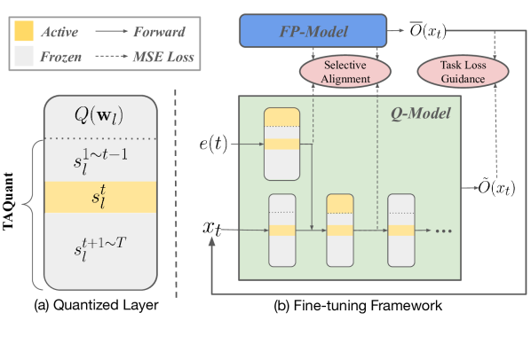
Addressing the revealed properties, we propose a novel quantization approach for diffusion models, termed QuEST (Quantization via Efficient Selective FineTuning). Confronting property ❶ , we first theoretically justify that weight finetuning can enhance model robustness towards large perturbations under low-bit settings for reducing quantization error, whereas previous methods struggle to find appropriate quantization parameters. Then we empirically show that by finetuning the model, the activation distributions are actually modified to be more amenable to quantization. Following the idea of weight finetuning, we identify two types of layers that are responsible for performance degradation: Time embedding layers exhibiting property ❷ and attention-related layers corresponding to property ❸ . Thus, we selectively and progressively finetune these small layer subsets in conjunction with all activation quantization parameters, as illustrated in Figure 1(b). With less than 10% of the total parameters involved, QuEST not only substantially enhances low-bit quantized model performance, but is also notably time-efficient and requires only supervision from the full-precision model in a data-free manner. To preserve the essential time information, we further introduce an efficient Time-aware Activation Quantizer (shown in Figure 1(a)) that can flexibly adapt to the varying activation distributions over the numerous time steps. Our contributions are summarized as follows:

• We uncover and validate three properties that present challenges to low-bit diffusion model quantization. We also theoretically discuss why previous methods are expected to fail and justify the sufficiency of weight finetuning under low-bit settings.

• Addressing the identified properties, we introduce QuEST, an innovative finetuning strategy that trains the model selectively and progressively, achieving low-bit quantization capability with high time and memory efficiency. An efficient activation quantizer is also proposed for effective time information estimation. Practically, our method can be executed in a data-free and parameter-efficient manner.

• Experiments on three high-resolution image generation tasks over four models demonstrate the superiority of our method, achieving state-of-the-art performance under various bit-width settings. We are also the first method to generate reasonable images for full 4-bit Stable Diffusion.

Figure 1: Framework of the proposed method at time step $t$. $s_{l}^{t}$ represents the quantization parameters of layer $l$ at time $t$, $Q(\textbf{w}_{l})$ represents the quantized weight of layer $l$. (a) In a quantized layer, the scaling factor $s_{l}^{t}$ is updated while the others are frozen at time $t$. (b) $e(t)$ and $x_{t}$ are the input time embedding and input image representation respectively. The model layers’ weights are optimized selectively and the quantization parameters are all updated. While different selected layers are learned progressively, the corresponding weight and scaling factors are updated simultaneously using intermediate activation alignment and task loss guidance.

2 Related Work

2.1 Diffusion Model Inference

Diffusion models (Ho et al., 2020; Rombach et al., 2021) generate samples via a learned iterative denoising process. During inference, the initial input is sampled from a Gaussian distribution: $x_{T}\sim\mathcal{N}(\mathbf{0},\mathbf{I})$, and the final output $x_{0}$ is obtained by removing noises from $x_{T}$ subsequently using:

$$p_{\theta}(x_{t-1}|x_{t})=\mathcal{N}(x_{t-1};\tilde{\boldsymbol{\mu}}_{\theta,t}(x_{t}),\tilde{\beta_{t}}\mathbf{I}).$$ (1)

In this Markov Chain, $\tilde{\boldsymbol{\mu}}_{\theta,t}$ and $\tilde{\beta_{t}}$ are calculated from the model’s output. For a typical diffusion model, the denoising stage requires hundreds to thousands of iterations. This laborious sequential process makes efficient inference and high-resolution generation extremely challenging. Latent Diffusion Models (LDMs) (Rombach et al., 2021) were developed to overcome the challenges. They encode the data into a latent space and then apply the diffusion process within this space, enabling high-resolution image generation with fewer time steps. The output images are produced by decoding the latent representations. LDM’s concept and network quantization complement each other, mutually enhancing the efficiency of diffusion models.

Practically, diffusion models typically adopt a UNet architecture (Ronneberger et al., 2015), with some modules substituted by attention blocks. In a latent diffusion model, an encoder and a decoder are incorporated for projecting images into latent representations and subsequently generating images from the latent space, respectively. Usually encoders and decoders are lightweight and computationally inexpensive, so our focus is on quantizing the UNets in LDMs, in alignment with other works (as described below).

Table 1: Comparison with Different Quantization Frameworks.

Method	Data	Time & Memory	Low-bit
	Free	Efficient	Compatible
PTQ	✔	✔	✗
QAT	✗	✗	✔
Ours	✔	✔	✔

2.2 Diffusion Model Quantization

Model quantization is a dominant technique for optimizing the inference memory and speed of deep learning models by reducing the precision of the tensors used in computation. Few researches were done for quantizing diffusion models and they fall into two mainstream frameworks: Quantization-Aware Training (QAT) (Jacob et al., 2017; Li et al., 2022; Xu et al., 2023; Li et al., 2023b) and Post-Training Quantization (PTQ) (Wang et al., 2020; Nahshan et al., 2021; Li et al., 2021; Wei et al., 2023a; Liu et al., 2023). QAT methods such as Q-DM (Li et al., 2023b) consider value precision as an additional optimization constraint, training all parameters from scratch with the target task objective. While it is effective for low-bit quantization, it is even more resource-intensive than training a full-precision model. Efficient-DM (He et al., 2023a) further uses Low-rank adapters (LoRA) (Hu et al., 2021) to reduce training cost. However, it introduces extra weight parameters and still requires substantial training iterations.

Post-Training Quantization methods aim to calibrate the quantization parameters based on a small calibration set. Pioneering works such as PTQ4DM (Shang et al., 2023) and Q-Diffusion (Li et al., 2023a) focus on sampling the outputs of the full-precision model under different time steps with certain probabilities to construct the calibration set. ADP-DM (Wang et al., 2023) partition time steps into different groups and optimize each group with differentiable search algorithms. PTQ-D (He et al., 2023b) decomposes the quantization noise and correct them individually with full-precision model statistics. However, these methods generally fail under 4-bit or lower bit-width. To enable low-bit compatibility with high efficiency, our method adopts the general framework of PTQ but further introduces an efficient weight fine-tuning strategy. Table 1 shows the unique capabilities of our method, where we are able to realize QAT ability with PTQ efficiency.

3 Methodology

3.1 Preliminaries

The quantization process for a single value $x$ in a vector can be formulated as:

$$\hat{x} =\text{clamp}(\text{round}(\frac{x}{s})+Z;q_{min},q_{max}),$$ (2)

where $\hat{x}$ is the quantized integer result, $\text{round}(\cdot)$ represents rounding algorithms such as the round-to-nearest operator (Li et al., 2021) and AdaRound (Nagel et al., 2020), $s$ is referred to as the scaling factor and $Z$ is the zero-point. clamp is the function that clamps values into the range of $[q_{min},q_{max}]$, which is determined by the bit-width. Reversely, transforming the quantized values back into the full-precision form is formulated as:

$$\tilde{x}=(\hat{x}-Z)*s.$$ (3)

This is denoted as the dequantization process. The quantization and dequantization processes are performed on both model weights and layer outputs (also termed as ’activation’). Equation 2 indicates that the quantization error is composed of two factors: The clipping error produced by range clamping and the rounding error caused by the rounding function, where they exhibit a trade-off relationship (Li et al., 2021). While previous approaches strive for an optimal balance between the two errors, they neglect the intrinsic mechanisms in quantized diffusion models. In the next section, we investigate three properties of diffusion models that relate to quantization performance and show why typical quantization methods tend to fail.

3.2 Quantization-aware Properties of Diffusion Models

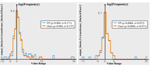
Property ❶ : The activation outputs are likely to have a majority of values close to zero, with the other values being numerically large and important. Previous works (Shang et al., 2023; Li et al., 2023a) paid attention to the varying activation distribution over different time steps, but none of them focused on the activation distribution itself. As shown in Figure 2, we find that in some layers, though the majority of values are close to 0, there exists values that are relatively large and diverse. Take the bin plot on the left for example, the original activation values (blue line) ranges from [-10, 34] but with over 99% values between [-0.6, 1.7], posing difficulties in minimizing the clipping error. This phenomenon is different from the outlier distribution observed in LLMs (Lin et al., 2023; Xiao et al., 2023), where the outliers are always positive and show up at certain positions consistently (Wei et al., 2023b). Moreover, we observe that the larger values are important for generation performance. With the large values being important and the small values appearing frequently, neither of them are negligible and need to be carefully quantized at the same time. Unfortunately, typical quantization methods fall short of this ability under low-bit settings, where the rounding error often outweighs the clipping error during optimization and results in over-clipped large values, generating corrupted images. This phenomenon inspires us to reshape the activation distributions via model finetuning to attain more quantization-friendly distributions.

Figure 2: Illustrations of imbalanced activation distributions. We cluster activation values into uniformly distributed bins and manipulate the frequency for better visualization. In the activation distribution of the full-precision model, the majority of values cluster near zero with sporadic large values, presenting challenges for low-bit quantization. Our method reduces the large values to enable easier quantization for improved performance.

Property ❷ : Accurate temporal information is critical for quantized diffusion model performance. As shown in Equation 1, diffusion model predictions are highly correlated with time step information. Specifically, time steps are transformed and projected into time embeddings and then added onto the image features, guiding the model to denoise correctly. Table 2 shows the performance comparison of quantizing time embeddings or preserving their full-precision values in the LDM-4 of LSUN-Bedrooms (Yu et al., 2015). Under W8A8 and W4A8, quantizing the time embeddings leads to an increase of 0.81 and 1.04 (relatively 15%) in FID, respectively. This indicates that inaccurate time embedding quantization can lead to large degradation in generation performance, yielding even larger corruptions under lower bit-widths. Due to the different focus diffusion models have on image generation at different time steps, we infer that inaccurate time embeddings can cause mismatched input image and model functionality, resulting in possible oscillations in the sequence of noise removal. Thus, preserving diffusion model performance under quantization requires accurate temporal information.

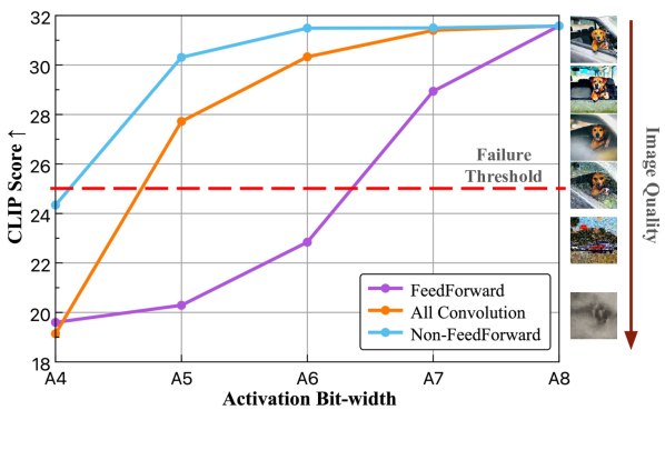
Property ❸ : Different activations have different sensitivity towards decreasing bit-width. Low-bit activation quantization is often more difficult than weight quantization and remains the key challenge for diffusion model quantization. Compared with weights than can be categorized into linear layers and convolutional layers, activation types are more diverse and complicated. We hence examine the effects on model performance when quantizing different activations. Figure 3 shows how sensitive different activations are to quantization in Stable Diffusion. We quantize three different types of activations to lower bits while maintaining the others’ bit-width (8-bit). We observe that the FeedForward layer (Feng et al., 2023) activations cause generation failure at 6 bits, whereas the activations of all other linear layers (containing 5 times more layers) barely fail at 4 bits and all convolution layers (containing 3 times more layers) only fail at 4 bits. This phenomenon indicates that a small amount of activations are especially sensitive to low-bit quantization, making them essential to be specially dealt with.

Table 2: FP & Quantized Time Embedding Comparisons.

Settings	FID $\downarrow$	sFID $\downarrow$
W8A8 (Quantized Time Embedding)	7.58	22.07
W8A8 (FP Time Embedding)	6.77	22.03
W8A8 (TAQuant+$\text{SLA}_{\text{TE}}$)	5.61	21.22
W4A8 (Quantized Time Embedding)	8.59	22.74
W4A8 (FP Time Embedding)	7.55	21.69
W4A8 (TAQuant+$\text{SLA}_{\text{TE}}$)	6.95	23.17

3.3 Quantization via Efficient Selective Finetuning

In this section, we first theoretically discuss the potential reasons for the failure of previous methods and the underlying rationale for weight fine-tuning. Then we introduce a finetuning method QuEST for diffusion models that can significantly boost low-bit performance with less time and memory usage. Figure 1 illustrates the proposed framework, which is a distillation-based finetuning strategy consisting of selective weight optimization and network-wise scaling factor optimization. To further address the loss of temporal information due to quantization, we propose an efficient time-aware activation quantizer.

3.3.1 Sufficiency of Finetuning

We first review the underlying theoretical foundation underpinning previous methods, which typically employ the reconstruction-based post-training quantization approach. Denote the diffusion model’s activations at time $t$ as $\mathbf{z}_{t}=[z_{1,t},z_{2,t},...,z_{n,t}]$, the task loss as $L(z_{n,t},\overline{z}_{n,t})$, where $n$ is the number of layers and $\overline{z}_{n,t}$ is the ground-truth. $L$ can be any loss function and here we use the mean squared error (MSE). We treat quantization as a type of perturbation and formulate the influence of activation quantization using Taylor expansion, assuming model weight $\mathbf{w}$ is frozen:

$$\mathbb{E}[L(z_{n,t} +\Delta;\mathbf{w})]-\mathbb{E}[L(z_{n,t};\mathbf{w})]$$

$$\approx\Delta^{T}\overline{\mathbf{g}}^{(z_{n,t})}+\frac{1}{2}\Delta^{T}\overline{\mathbf{H}}^{(z_{n,t})}\Delta,$$ (4)

where $\Delta$ is the activation perturbation, $\overline{\mathbf{g}}^{(\mathbf{z})}$ is the gradient and $\overline{\mathbf{H}}^{(z_{n,t})}$ is the Hessian matrix. According to (Li et al., 2021; Yuan et al., 2022), for a well-trained model, $\overline{\mathbf{g}}^{(z_{n,t})}=\nabla_{z_{n,t}}L$ approaches $0$. Thus the above equation can be simplified to:

$$\mkern-18.0mu\frac{1}{2}\Delta^{T}\overline{\mathbf{H}}^{(z_{n,t})}\Delta=\frac{1}{2}(\tilde{z}_{n,t}-z_{n,t})^{T}\overline{\mathbf{H}}^{(z_{n,t})}(\tilde{z}_{n,t}-z_{n,t}).\mkern-18.0mu$$ (5)

This leads to a rather straightforward conclusion: Quantization error can be reduced by reconstructing the model output. However, under low-bit settings, the reasoning from Equation 3.3.1 to Equation 5 is inaccurate, where the activation perturbation $\Delta$ is too large for meaningful Taylor expansion. Thus we have the following proposition:

Proposition 3.1.

Reconstruction-based post-training quantization methods may lose their theoretical guarantee due to the large value perturbations under low-bit quantization.

To resolve the above problem, we can use the following theorem by transforming $\Delta$ into a smaller perturbation $\epsilon$:

Theorem 3.2.

Given an $n$ layer diffusion model at time $t$ with quantized activations as $\tilde{\mathbf{z}}_{t}=[\tilde{z}_{1,t},\tilde{z}_{2,t},...,\tilde{z}_{n,t}]$ and $\tilde{z}_{n,t}=z_{n,t}+\Delta$, where $z_{n,t}$ is the ground-truth and $\Delta$ is the large perturbation caused by low-bit quantization. Denote the target task MSE loss as $L(\tilde{z}_{n,t},\overline{z}_{n,t})$, the quantization error can be transformed into:

$$\mathbb{E}[L(z_{n,t}+\Delta;\mathbf{w})]-\mathbb{E}[L(z_{n,t};\mathbf{w})]$$

$$\approx 2\epsilon^{T}\sum_{i=1}^{K}(\tilde{z}_{n-1,t}^{i}\cdot\mathbf{w}_{n}-z_{\text{FP}})$$

$$+\frac{1}{2}\sum_{i=1}^{K}(\tilde{z}_{n,t}^{i}-z_{\text{FP}})^{T}\overline{\mathbf{H}}^{(z_{n,t}+(i-1)\epsilon)}(\tilde{z}_{n,t}^{i}-z_{\text{FP}})$$ (6)

where $\mathbf{w}_{n}$ is the weight for layer $n$ and $\tilde{z}_{n,t}^{i}=\tilde{z}_{n-1,t}^{i}\cdot\mathbf{w}_{n}$, $\epsilon$ is a perturbation small enough for Taylor expansion, $K$ is a constant and $\Delta=K\epsilon$.

Theorem 3.2 indicates that: To minimize the quantization error, ideally we can finetune $\mathbf{w}_{n}$ so that for any $i$, the weights can fit to the data/activation $\tilde{z}_{n-1,t}^{i}+(i-1)\epsilon$ which the full-precision counterpart may not fit, making the model more robust to varying inputs. In other words, we are finetuning the model weights for better robustness towards large input activation perturbations, therefore enabling easier quantization. We also find that the second term in Equation 3.2 can be minimized simultaneously with the first term, so that the total quantization error can be reduced via a common goal: Activation output alignment via finetuning $\mathbf{w}_{n}$.

Figure 3: Effect of decreasing different activations’ bit-width on the model performance in Stable Diffusion. FeedForward layers experience generation failures at 6 bits, while all other linear layers barely fail at 4 bits and all convolution layers only fail at 4 bits.

3.3.2 Quantization via Selective Finetuning

Motivated by the unraveled properties of quantized diffusion models and the shortcomings in existing quantization approaches, we propose an efficient finetuning strategy for low-bit diffusion model quantization. The components of our method are detailed below.

Data-Free Partial-network-wise Training. To alleviate the need of substantial training data, we propose to adopt the general setting of Post-Training Quantization and construct the calibration set in a data-free manner. By feeding sampled Gaussian noises $x_{T}$ into the full-precision model and sample iteratively over different time steps using Equation 1, we can obtain the calibration data needed for finetuning the quantized model. In practice, the number of samples generated for each time step is 256, indicating that we only have to inference the full-precision model a few times to obtain the needed number of calibration samples.

Moreover, inspired by the fact that we can view the activation quantization parameters as additional model parameters which all contribute to the final output, we propose a partial-network-wise training strategy. Different from quantization methods using layer-wise or block-wise reconstruction (Shang et al., 2023; Li et al., 2023a) that binds quantization parameters with their corresponding layers or blocks, we optimize all activation scaling factors for each time step and only train partial weight parameters (e.g. 7% of the parameters in LDM-4). As depicted in Figure 1, the majority of the model weights remain unchanged at time step $t$, and only a small subset of parameters (including layer weights and scaling factors) related to this time step are updated using the full-precision model’s outputs as ground-truth. The choices for the weights to be finetuned are discussed in the following sections. Additionally, while layer/block-wise optimization methods can only reconstruct sequentially, our approach update the required parameters at once. In this way, we significantly save the time and memory needed for quantization. Note that the quantization parameters for the weights are not updated once initialized, in order to maintain memory efficiency during deployment.

Table 3: Unconditional image generation results of LDM-4 models on LSUN-Bedrooms/Churches 256$\times$256. ”N/A” denotes generation failure. ”FP” denotes the full precision model.

Dataset	Method	Bit-width (W/A)	Size (MB)	FID$\downarrow$
LSUN- Bedrooms (LDM-4)	FP	32/32	1045.6	2.95
	PTQ4DM	8/8	279.1	4.75
	Q-Diffusion	8/8	279.1	4.53
	PTQ-D	8/8	279.1	3.75
	Ours	8/8	279.1	3.07
	PTQ4DM	4/8	148.4	-
	Q-Diffusion	4/8	148.4	5.37
	PTQ-D	4/8	148.4	5.94
	Ours	4/8	148.4	3.26
	PTQ4DM	4/4	148.4	N/A
	Q-Diffusion	4/4	148.4	N/A
	PTQ-D	4/4	148.4	N/A
	Ours	4/4	148.4	5.64
LSUN- Churches (LDM-8)	FP	32/32	1125.4	4.02
	PTQ4DM	8/8	330.6	5.54
	Q-Diffusion	8/8	330.6	6.94
	PTQ-D	8/8	330.6	6.40
	Ours	8/8	330.6	6.55
	PTQ4DM	4/8	189.9	-
	Q-Diffusion	4/8	189.9	7.80
	PTQ-D	4/8	189.9	7.33
	Ours	4/8	189.9	7.33
	PTQ4DM	4/4	189.9	N/A
	Q-Diffusion	4/4	189.9	N/A
	PTQ-D	4/4	189.9	N/A
	Ours	4/4	189.9	11.76

Efficient Time-aware Activation Quantization. Temporal information is a unique and essential factor in diffusion models. As highlighted in (Shang et al., 2023; Li et al., 2023a), the variation of activation distribution over different time steps is fatal for conventional PTQ methods. Also, as discussed in Section 3.2, accurate time embedding quantization is critical. To discriminate between different time steps, we design the Time-aware Activation Quantizer (TAQuant) that adopts different sets of activation quantization parameters for different time steps. While these parameters consumes negligible memory and does not effect inference speed, learning independent parameters for each time step leads to immense time cost. Inspired by the fact that neighboring time steps yield similar functions in diffusion models (Choi et al., 2022), we use the simple strategy of clustering neighboring time steps so that they share the same calibration data and quantization parameters. Then the set of activation quantization parameters are formulated as:

$$\mathbf{s}=\{\mathbf{s}^{t}(x_{t}),\mathbf{s}^{2t}(x_{2t}),...,\mathbf{s}^{T}(x_{T})\},$$ (7)

where the time steps used for optimization are sampled uniformly, and each chosen time step’s statistics are used to represent $T/t$ adjacent ones. Though most time steps’ quantization parameters are approximated, this strategy saves the optimization time by $t$ times without compromising much performance. Section 4.3 further provides an analysis on the trade-off between time efficiency and model performance.

Selective & Progressive Layer Alignment. As investigated in Section 3.2, we identify two crucial types of activations for image generation performance and select them for weight finetuning: Time embeddings and attention-related activations (e.g. FeedForward layers in Stable Diffusion). We progressively update these components due to their distinct, non-overlapping functionalities.

Table 4: Class-conditional image generation results of the LDM-4 model on ImageNet 256$\times$256, containing 1,000 categories.

Bit-width (W/A)	Method	Size (MB)	FID$\downarrow$	sFID$\downarrow$	IS$\uparrow$
32/32	FP	1529.7	11.28	7.70	364.73
8/8	Q-Diffusion	428.7	10.60	9.29	350.93
	PTQ-D	428.7	10.05	9.01	359.78
	Ours	428.7	10.43	6.07	365.12
4/8	Q-Diffusion	237.5	9.29	9.29	336.80
	PTQ-D	237.5	8.74	7.98	344.72
	Ours	237.5	8.48	6.55	346.02
4/4	Q-Diffusion	237.5	N/A	N/A	N/A
	PTQ-D	237.5	N/A	N/A	N/A
	Ours	237.5	5.98	7.93	202.45

Table 5: Text-to-image generation results (512$\times$512) of Stable Diffusion v1.4 using COCO2014 validation set prompts.

Bit-width (W/A)	Method	Size (MB)	CLIP Score$\uparrow$
32/32	FP	3279.1	31.50
8/8	Q-Diffusion	949.0	31.43
	Ours	949.0	31.47
4/8	Q-Diffusion	539.1	31.39
	Ours	539.1	31.50
4/4	Q-Diffusion	539.1	N/A
	Ours	539.1	28.85

Figure 4: Generated images compared with Q-Diffusion under two bit-width types: W8A8 and W4A4, using LDM-4 in LSUN-Bedrooms. Our method not only succeed well in generating low-bit images, but also aligns more closely with the full-precision counterpart.

During a single forward process, identical time embeddings are injected into different parts of the model, passed through projection layers, and merged with the latent image representations. This implies that the time information operates independently from the primary network flow. Thus, we first refine the time embedding layer $l$’s weight $\mathbf{w}_{l}$ along with its activation quantization parameters $\mathbf{s}_{l}^{t}$ using:

$$\mathcal{L}_{\text{TE}}^{t}=\sum_{l\in\mathbb{C}_{\text{TE}}}\mathbb{E}_{t}[||\overline{O}(e(t);\mathbf{w}_{l})-\tilde{O}(e(t);\mathbf{w}_{l},\mathbf{s}_{l}^{t})||^{2}],$$ (8)

where $\mathbb{C}_{\text{TE}}$ represents the set of time embedding layers, $e(t)$ is the fixed time embedding for time $t$, $\overline{O}(e(t);\mathbf{w}_{l})$ is the activation output of the full-precision model representing the ground-truth, and $\tilde{O}(e(t);\mathbf{w}_{l},\mathbf{s}_{l}^{t})$ is the quantized output. This loss function indicates that the chosen weight parameters are consistently updated across different time steps to ensure robustness to diverse inputs, whereas only the subset of scaling factors relevant to each specific time step are adjusted for temporal information discrimination.

Apart from time embedding layers, attention-related layers are also vital. As depicted in Figure 3, reducing activation bit-width of these layers degrades model performance the most dramatically. Denote $\mathbb{C}_{\text{A}}$ as the set containing all these layers and given the image calibration samples $x_{t}$, we optimize $\mathbf{w}_{l}$ and $\mathbf{s}^{t}$ but exclude the quantization parameters already optimized in Equation 8:

$$\mkern-18.0mu\mathcal{L}_{\text{A}}^{t}=\sum_{l\in\mathbb{C}_{A}}\mathbb{E}_{t}[||\overline{O}(x_{t};\mathbf{w}_{:l})-\tilde{O}(x_{t};\mathbf{w}_{:l},\mathbf{s}^{t}\setminus s_{\mathbb{C}_{\text{TE}}}^{t})||^{2}],\mkern-18.0mu$$ (9)

where $\mathbf{w}_{:l}$ are the weight parameters of the first $l$ layers. This strategy resembles linear probing, where only the layer directly associated with the activation output is finetuned.

Furthermore, we aim not only for each independent layer’s quantization error reduction, but also for the final generated images’ quality improvement. Therefore, the target task loss $\sum_{t}\mathcal{L}_{d}^{t}$ is introduced, where the ground-truth is approximated by the output of the full-precision counterpart. By integrating Equation 8 and Equation 9, the final objective is formulated as follows:

$$\mathcal{L} =\sum_{t}((\mathcal{L}_{\text{TE}}^{t}+\mathcal{L}_{d}^{t})+(\mathcal{L}_{\text{A}}^{t}+\mathcal{L}_{d}^{t}))$$

$$=\sum_{t}(\mathcal{L}_{\text{TE}}^{t}+\mathcal{L}_{\text{A}}^{t}+2\mathbb{E}[||\overline{O}(x_{t};\mathbf{w})-\tilde{O}(x_{t};\mathbf{w},\mathbf{s}^{t})||^{2}]).$$ (10)

4 Experiments

4.1 Experiment Settings

To verify the effectiveness of our proposed method, we conduct experiments on three types of generation tasks: Unconditional image generation on LSUN-Bedrooms and LSUN-Churches datasets (Yu et al., 2015), class-conditional image generation on ImageNet (Deng et al., 2009), and text-to-image generation. The model architectures we quantize include LDM and Stable Diffusion (Rombach et al., 2021), and uses ”WnAm” to represent the quantization setting: n-bit weight quantization and m-bit activation quantization. DDIM samplers (Ho et al., 2020) are adopted for LDMs and the PLMS sampler (Liu et al., 2022) is used for Stable Diffusion. We generate 256 samples per time step for constructing the calibration set, and train 20 epochs over each time step. The Adam optimizer (Kingma & Ba, 2017) is adopted and the learning rate for weight finetuning and scaling factor finetuning are set as $1e^{-5}$ and $1e^{-4}$ respectively.

The performance of different quantized LDMs are evaluated using the Fr$\acute{\text{e}}$chet Inception Distance (FID) (Heusel et al., 2018), spatial FID (sFID) (Nash et al., 2021) and Inception Score (IS) (Barratt & Sharma, 2018). Unless specified, quantitative results are obtained by sampling 50,000 images from the models and evaluated using the official evaluation scripts (Dhariwal & Nichol, 2021). For Stable Diffusion, we use the CLIP Score (Hessel et al., 2022) for evaluation.All experiments are conducted on A6000 GPUs using the PyTorch framework (Paszke et al., 2019).

4.2 Experiment Results

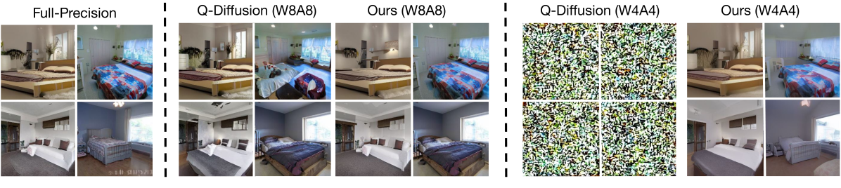
Unconditional Generation: We evaluate the performance of our method over LDM-4 (LSUN-Bedrooms 256$\times$256) and LDM-8 (LSUN-Churches 256$\times$256) using the DDIM sampler with 200 and 500 time steps, respectively. Results are shown in table 3. We compare with methods including PTQ4DM (Shang et al., 2023), Q-Diffusion (Li et al., 2023a) and PTQ-D (He et al., 2023b). The results are evaluated using FID, where the Inception Score is not a reasonable metric for datasets that have significantly different domains and categories from ImageNet (Li et al., 2023a).

Table 6: Different component comparison and efficiency comparison on LDM-4 (LSUN-Bedrooms 256 $\times$ 256).

Method	Bit-width (W/A)	Calibration data size	Time cost (GPU hours)	Memory cost (MB)	Model size (MB)	FID$\downarrow$
FP	32/32	-	-	-	1045.6	2.95
PTQ (Li et al., 2023a)	4/4	5120	23.08	10334	148.4	428.8
TAQuant	4/4	5120	11.52	9822	148.4	12.56
+ $\text{SLA}_{\text{TE}}$	4/4	5120	13.13	12134	148.4	6.41
+ $\text{SLA}_{\text{A}}$	4/4	5120	15.25	12450	148.4	5.78

Class-conditional Generation: We evaluate the performance using LDM-4 on ImageNet 256$\times$256 using the DDIM sampler (20 steps). As shown in Table 4, three metrics are used for evaluation. Note that sFID uses additional intermediate spatial features for calculation compared with FID. We can also see that FID is not a valid metric for ImageNet LDM-4 evaluation: All methods have lower FID when quantized to lower-bits, conflicting with human perception. We show that our method not only succeeds in W4A4 quantization, but also significantly improve the generation quality on higher bit settings. Under W8A8, our method is able to achieve 2.82 improvement over sFID and 8.13 increase in Inception Score. Under W4A8, we improve the SOTA PTQ method by 1.57 sFID and 8.77 IS.

Text-to-image Generation: We use Stable Diffusion v1.4 as the model for quantization with the PLMS sampler sampling 50 time steps. Table 5 shows the results. Images are generated based on the 10,000 prompts sampled from the COCO2014 (Lin et al., 2015) validation set, and CLIP Score is calculated based on the ViT-B/16 backbone. Given the limited works done on Stable Diffusion, we can only compare with Q-Diffusion and the full-precision baseline.

4.3 Experimental Analysis

Efficiency comparison and effects of different component. In Table 6, we present a comparison of efficiency between our method and the post-training quantization approach on the LSUN-Bedrooms dataset. Our approach, while utilizing the same quantity of calibration data as the PTQ method, is more time-efficient and incurs only a 20% increase in memory usage. We also show how each proposed component improves the generation performance. The results indicate that sequentially finetuning time embedding layers followed by attention-related layers leads to consistent improvements in model performance.

Table 7 presents the comparison of with and without the use of task loss $\mathcal{L}_{d}$. The results show that using the difference between the outputs of the quantized model and the full-precision counterpart for supervision is essential for performance improvement, enhancing the FID by 2.58 and 5.21 for $\text{SLA}_{\text{TE}}$ and $\text{SLA}_{\text{A}}$, respectively. However, when the learning process is only supervised by the task loss, the performance degrades by 7.13 FID and 9.39 sFID for $\text{SLA}_{\text{TE}}$, indicating that the task loss alone is insufficient.

Table 7: Influence of task loss supervision on model performance.

Method	$\text{SLA}_{\text{TE}}$ w/o $\mathcal{L}_{d}$	$\text{SLA}_{\text{TE}}$ w/ $\mathcal{L}_{d}$	$\text{SLA}_{\text{A}}$ w/o $\mathcal{L}_{d}$	$\text{SLA}_{\text{A}}$ w/ $\mathcal{L}_{d}$
FID$\downarrow$	8.99	6.41	11.41	6.20
sFID$\downarrow$	15.23	11.18	15.64	12.32

Time step sampling frequency analysis. While time steps are sampled uniformly, will the performance consistently improve when we sample more frequently? Table 8 illustrates the trade-off between the increased number of sampled time steps (’T-Num’) and generation performance. Metrics are calculated using 10,000 samples generated from LDM-4 on LSUN-Bedrooms. The results show that the though performance improves consistently, the amount of growth gradually decreases. Starting from 5 time steps, using 15 more time steps leads to 25.22 sFID improvement. But using another 30 time steps (from 20 to 50) only leads to 2.92 sFID improvement. Given the linearly increasing time cost associated with using more time steps, we opt for only 20 out of 200 time steps to enhance quantization efficiency.

Table 8: Effect of number of uniformly sampled time steps for W4A4 LDM-4 on LSUN-Bedrooms dataset.

T-Num	5	10	20	25	40	50
FID $\downarrow$	19.34	15.27	12.56	12.16	11.04	10.54
sFID $\downarrow$	54.00	37.47	28.78	27.99	26.42	25.86

How QuEST influences model properties. Our approach is based on the certain characteristics observed in quantized diffusion models, hence we aim to analyze how our fine-tuning strategy counters these identified challenges. As shown in Table 2, finetuning time embedding layers leads to even better performance than the full-precision counterpart. We infer that this might be due to both the additional parameters introduced by quantization and the additional task loss supervision. Figure 2 further implies that our method adjusts the activation distribution so that it can be more easily quantized. We see that the ranges of the activation value distributions shrink from [-10, 34] to [-4, 14] and [-11, 20] to [-4, 4]. The standard deviations also decrease from 0.171 to 0.157 and from 0.073 to 0.071. This indicates a higher concentration of values around the mean, which can effectively reduce both rounding and clipping errors.

5 Conclusion

In this work, we propose QuEST, an efficient data-free finetuning framework for low-bit diffusion model quantization. Our method is motivated by the three underlying properties found in quantized diffusion models. We also theoretically demonstrate the sufficiency of finetuning, interpreting it as a way to enhance model robustness against large activation perturbations. To alleviate the performance degradation, we propose to finetune the time embedding layers and attention-related layers under the supervision of the full-precision counterpart. A time-aware activation quantizer is also introduced to handle varying time steps. Experimental results over three high-resolution image generation tasks demonstrate the effectiveness and efficiency of QuEST, achieving low-bit compatibility with less time and memory cost.

References

- Barratt & Sharma (2018) Barratt, S. and Sharma, R. A note on the inception score, 2018.
- Chitty-Venkata et al. (2023) Chitty-Venkata, K. T., Mittal, S., Emani, M., Vishwanath, V., and Somani, A. K. A survey of techniques for optimizing transformer inference. Journal of Systems Architecture, pp. 102990, 2023.
- Choi et al. (2022) Choi, J., Lee, J., Shin, C., Kim, S., Kim, H., and Yoon, S. Perception prioritized training of diffusion models, 2022.
- Croitoru et al. (2023) Croitoru, F.-A., Hondru, V., Ionescu, R. T., and Shah, M. Diffusion models in vision: A survey. IEEE Transactions on Pattern Analysis and Machine Intelligence, 45(9):10850–10869, 2023.
- Deng et al. (2009) Deng, J., Dong, W., Socher, R., Li, L.-J., Li, K., and Fei-Fei, L. Imagenet: A large-scale hierarchical image database. In 2009 IEEE conference on computer vision and pattern recognition, pp. 248–255. IEEE, 2009.
- Dhariwal & Nichol (2021) Dhariwal, P. and Nichol, A. Diffusion models beat gans on image synthesis, 2021.
- Dosovitskiy et al. (2021) Dosovitskiy, A., Beyer, L., Kolesnikov, A., Weissenborn, D., Zhai, X., Unterthiner, T., Dehghani, M., Minderer, M., Heigold, G., Gelly, S., Uszkoreit, J., and Houlsby, N. An image is worth 16x16 words: Transformers for image recognition at scale, 2021.
- Feng et al. (2023) Feng, Z., Zhang, Z., Yu, X., Fang, Y., Li, L., Chen, X., Lu, Y., Liu, J., Yin, W., Feng, S., Sun, Y., Chen, L., Tian, H., Wu, H., and Wang, H. Ernie-vilg 2.0: Improving text-to-image diffusion model with knowledge-enhanced mixture-of-denoising-experts. In Proceedings of the IEEE/CVF Conference on Computer Vision and Pattern Recognition (CVPR), pp. 10135–10145, June 2023.
- Gholami et al. (2022) Gholami, A., Kim, S., Dong, Z., Yao, Z., Mahoney, M. W., and Keutzer, K. A survey of quantization methods for efficient neural network inference. In Low-Power Computer Vision, pp. 291–326. Chapman and Hall/CRC, 2022.
- He et al. (2015) He, K., Zhang, X., Ren, S., and Sun, J. Deep residual learning for image recognition, 2015.
- He et al. (2023a) He, Y., Liu, J., Wu, W., Zhou, H., and Zhuang, B. Efficientdm: Efficient quantization-aware fine-tuning of low-bit diffusion models, 2023a.
- He et al. (2023b) He, Y., Liu, L., Liu, J., Wu, W., Zhou, H., and Zhuang, B. Ptqd: Accurate post-training quantization for diffusion models, 2023b.
- Hessel et al. (2022) Hessel, J., Holtzman, A., Forbes, M., Bras, R. L., and Choi, Y. Clipscore: A reference-free evaluation metric for image captioning, 2022.
- Heusel et al. (2018) Heusel, M., Ramsauer, H., Unterthiner, T., Nessler, B., and Hochreiter, S. Gans trained by a two time-scale update rule converge to a local nash equilibrium, 2018.
- Ho et al. (2020) Ho, J., Jain, A., and Abbeel, P. Denoising diffusion probabilistic models, 2020.
- Hu et al. (2021) Hu, E. J., Shen, Y., Wallis, P., Allen-Zhu, Z., Li, Y., Wang, S., Wang, L., and Chen, W. Lora: Low-rank adaptation of large language models, 2021.
- Jacob et al. (2017) Jacob, B., Kligys, S., Chen, B., Zhu, M., Tang, M., Howard, A., Adam, H., and Kalenichenko, D. Quantization and training of neural networks for efficient integer-arithmetic-only inference, 2017.
- Kingma & Ba (2017) Kingma, D. P. and Ba, J. Adam: A method for stochastic optimization, 2017.
- Li et al. (2023a) Li, X., Liu, Y., Lian, L., Yang, H., Dong, Z., Kang, D., Zhang, S., and Keutzer, K. Q-diffusion: Quantizing diffusion models. In Proceedings of the IEEE/CVF International Conference on Computer Vision (ICCV), pp. 17535–17545, October 2023a.
- Li et al. (2021) Li, Y., Gong, R., Tan, X., Yang, Y., Hu, P., Zhang, Q., Yu, F., Wang, W., and Gu, S. Brecq: Pushing the limit of post-training quantization by block reconstruction. arXiv preprint arXiv:2102.05426, 2021.
- Li et al. (2022) Li, Y., Xu, S., Zhang, B., Cao, X., Gao, P., and Guo, G. Q-vit: Accurate and fully quantized low-bit vision transformer, 2022.
- Li et al. (2023b) Li, Y., Xu, S., Cao, X., Zhang, B., and Sun, X. Q-dm: An efficient low-bit quantized diffusion model. In NeurIPS 2023, October 2023b.
- Liang et al. (2021) Liang, T., Glossner, J., Wang, L., Shi, S., and Zhang, X. Pruning and quantization for deep neural network acceleration: A survey. Neurocomputing, 461:370–403, 2021.
- Lin et al. (2023) Lin, J., Tang, J., Tang, H., Yang, S., Dang, X., Gan, C., and Han, S. Awq: Activation-aware weight quantization for llm compression and acceleration, 2023.
- Lin et al. (2015) Lin, T.-Y., Maire, M., Belongie, S., Bourdev, L., Girshick, R., Hays, J., Perona, P., Ramanan, D., Zitnick, C. L., and Dollár, P. Microsoft coco: Common objects in context, 2015.
- Liu et al. (2023) Liu, J., Niu, L., Yuan, Z., Yang, D., Wang, X., and Liu, W. Pd-quant: Post-training quantization based on prediction difference metric, 2023.
- Liu et al. (2022) Liu, L., Ren, Y., Lin, Z., and Zhao, Z. Pseudo numerical methods for diffusion models on manifolds, 2022.
- Nagel et al. (2020) Nagel, M., Amjad, R. A., Van Baalen, M., Louizos, C., and Blankevoort, T. Up or down? adaptive rounding for post-training quantization. In International Conference on Machine Learning, pp. 7197–7206. PMLR, 2020.
- Nahshan et al. (2021) Nahshan, Y., Chmiel, B., Baskin, C., Zheltonozhskii, E., Banner, R., Bronstein, A. M., and Mendelson, A. Loss aware post-training quantization. Machine Learning, 110(11-12):3245–3262, 2021.
- Nash et al. (2021) Nash, C., Menick, J., Dieleman, S., and Battaglia, P. W. Generating images with sparse representations, 2021.
- Paszke et al. (2019) Paszke, A., Gross, S., Massa, F., Lerer, A., Bradbury, J., Chanan, G., Killeen, T., Lin, Z., Gimelshein, N., Antiga, L., Desmaison, A., Köpf, A., Yang, E., DeVito, Z., Raison, M., Tejani, A., Chilamkurthy, S., Steiner, B., Fang, L., Bai, J., and Chintala, S. Pytorch: An imperative style, high-performance deep learning library, 2019.
- Pilipović et al. (2018) Pilipović, R., Bulić, P., and Risojević, V. Compression of convolutional neural networks: A short survey. In 2018 17th International Symposium INFOTEH-JAHORINA (INFOTEH), pp. 1–6. IEEE, 2018.
- Rombach et al. (2021) Rombach, R., Blattmann, A., Lorenz, D., Esser, P., and Ommer, B. High-resolution image synthesis with latent diffusion models, 2021.
- Ronneberger et al. (2015) Ronneberger, O., Fischer, P., and Brox, T. U-net: Convolutional networks for biomedical image segmentation, 2015.
- Shang et al. (2023) Shang, Y., Yuan, Z., Xie, B., Wu, B., and Yan, Y. Post-training quantization on diffusion models. In CVPR, 2023.
- Wang et al. (2023) Wang, C., Wang, Z., Xu, X., Tang, Y., Zhou, J., and Lu, J. Towards accurate data-free quantization for diffusion models, 2023.
- Wang et al. (2020) Wang, P., Chen, Q., He, X., and Cheng, J. Towards accurate post-training network quantization via bit-split and stitching. In International Conference on Machine Learning, pp. 9847–9856. PMLR, 2020.
- Wei et al. (2023a) Wei, X., Gong, R., Li, Y., Liu, X., and Yu, F. Qdrop: Randomly dropping quantization for extremely low-bit post-training quantization, 2023a.
- Wei et al. (2023b) Wei, X., Zhang, Y., Zhang, X., Gong, R., Zhang, S., Zhang, Q., Yu, F., and Liu, X. Outlier suppression: Pushing the limit of low-bit transformer language models, 2023b.
- Xiao et al. (2023) Xiao, G., Lin, J., Seznec, M., Wu, H., Demouth, J., and Han, S. Smoothquant: Accurate and efficient post-training quantization for large language models, 2023.
- Xu et al. (2023) Xu, S., Li, Y., Lin, M., Gao, P., Guo, G., Lu, J., and Zhang, B. Q-detr: An efficient low-bit quantized detection transformer, 2023.
- Yu et al. (2015) Yu, F., Zhang, Y., Song, S., Seff, A., and Xiao, J. Lsun: Construction of a large-scale image dataset using deep learning with humans in the loop. arXiv preprint arXiv:1506.03365, 2015.
- Yuan et al. (2022) Yuan, Z., Xue, C., Chen, Y., Wu, Q., and Sun, G. Ptq4vit: Post-training quantization framework for vision transformers with twin uniform quantization, 2022.