Efficient Solvers for Partial Gromov-Wasserstein

Abstract

The partial Gromov-Wasserstein (PGW) problem facilitates the comparison of measures with unequal masses residing in potentially distinct metric spaces, thereby enabling unbalanced and partial matching across these spaces. In this paper, we demonstrate that the PGW problem can be transformed into a variant of the Gromov-Wasserstein problem, akin to the conversion of the partial optimal transport problem into an optimal transport problem. This transformation leads to two new solvers, mathematically and computationally equivalent, based on the Frank-Wolfe algorithm, that provide efficient solutions to the PGW problem. We further establish that the PGW problem constitutes a metric for metric measure spaces. Finally, we validate the effectiveness of our proposed solvers in terms of computation time and performance on shape-matching and positive-unlabeled learning problems, comparing them against existing baselines.

1 Introduction

The classical optimal transport (OT) problem [48] seeks to match two probability measures while minimizing what is known as the expected transportation cost. At the heart of classical OT theory lies the principle of mass conservation, aiming to optimize the transportation from one probability measure to another under the premise that both measures maintain the same total mass, with strict preservation of mass throughout the transportation process. Statistical distances that arise from OT, such as the Wasserstein distances, have been widely applied across various machine learning domains, ranging from generative modeling [2, 26] to domain adaptation [14] and representation learning [30]. Notably, recent advancements have extended the OT problem to address certain limitations within machine learning applications. These advancements include: 1) facilitating the comparison of non-negative measures that possess different total masses via unbalanced [13] and partial OT [20], and 2) enabling the comparison of probability measures across distinct metric spaces through Gromov-Wasserstein distances [37], with applications spanning from quantum chemistry [24] to natural language processing [1].

Regarding the first aspect, many applications in machine learning involve comparing non-negative measures (often empirical measures) with varying total amounts of mass, e.g., domain adaptation [19]. Moreover, OT distances (or dissimilarity measures) are often not robust against outliers and noise, resulting in potentially high transportation costs for outliers. Many recent publications have focused on variants of the OT problem that allow for comparing non-negative measures with unequal mass. For instance, the optimal partial transport problem [9, 20, 21], Kantorovich–Rubinstein norm [25, 27, 32], and the Hellinger–Kantorovich distance [11, 33]. These methods fall under the broad category of “unbalanced optimal transport” [13, 33].

Regarding the second aspect, comparing probability measures across different metric spaces is essential in many machine learning applications, ranging from computer graphics, where shapes and surfaces are compared [8, 36], to graph partitioning and matching problems [50]. Source and target distributions often arise from varied conditions, such as different times, contexts, or measurement techniques, creating substantial differences in the intrinsic distances among data points. The conventional OT framework necessitates a meaningful distance across diverse domains, a requirement not always achievable. To circumvent this issue, the Gromov-Wasserstein (GW) distances were proposed in [36, 37] as an adaptation of the Gromov-Hausdorff distance, which measures the discrepancy between two metric spaces. The GW distance [37, 45] extends OT-based distances to metric measure spaces up to isometries. Its invariance across isomorphic metric measure spaces makes the GW distance particularly valuable for applications like shape comparison and matching, where invariance to rigid motion transformations is crucial.

Given that the Gromov-Wasserstein (GW) distance is limited to the comparison of probability measures, recent works have introduced unbalanced and partial variations of the GW distance [44, 10, 16]. These variations, known as unbalanced or partial GW problems, have been applied in diverse contexts, including partial graph matching [34] for social network analysis and the alignment of brain images [46].

Over the past decade, there has been extensive work on devising fast and efficient solvers for the OT problem and its unbalanced version, involving various techniques such as linear programming, Sinkhorn iterations, dynamic programming, and slicing (see, e.g., [25, 15, 38, 6, 5, 39, 12, 7, 3]). In the context of the Gromov-Wasserstein (GW) metric, the main computational challenge is the non-convexity of its formulation [37]. The conventional computational approach relies on the Frank-Wolfe (FW) Algorithm [23, 31]. In fact, OT computational methods (e.g. Sinkhorn algorithm) can be incorporated into FW iterations. This yields the classical GW solvers [40, 51, 47].

Motivated by the emerging applications of the partial GW (PGW) problem, this paper focuses on developing efficient solvers for it. We base our formulation of PGW on the general framework by [44], akin to the “Lagrangian form” of [10]’s mass-constraint approach, termed primal-PGW. Unlike [44], who introduce a KL-divergence penalty similar to the unbalanced OT problem and a Sinkhorn solver, we employ a total-variation penalty and present novel, efficient solvers for this problem. To the best of our knowledge, this is the first solution to the proposed PGW formulation in this paper.

Contributions. Our specific contributions in this paper

• Proposition 3.3. Analogous to [9]’s technique for turning the POT problem into an OT problem, here, we show that the partial Gromov-Wasserstein (PGW) problem can be turned into a variant of the Gromov-Wasserstein (GW) problem.

• Propositions 3.4 & 3.5. We demonstrate that $\left(PGW_{\lambda,q}(\cdot,\cdot)\right)^{\frac{1}{p}}$ is a metric between metric measure spaces and show that $\lambda$ provides an upper bound for allowed “transportation” cost.

• Solvers. We introduce two distinct solvers for the discrete PGW problem based on the Frank-Wolfe [23] algorithm. We show that these solvers are mathematically and computationally equivalent and they differ from previous solvers described by [10] and [44].

• Convergence Analysis. Inspired by the results of [31], we prove that, similar to the Frank-Wolfe solver presented in [10], our proposed solvers for the PGW problem converge linearly to a stationary point.

• Numerical Experiments. We demonstrate the performance of our proposed algorithms in terms of computation time and efficacy on two problems: shape-matching between 2D and 3D objects, and positive-unlabeled learning, and compare against baselines.

2 Background

Here, we review the basics of the OT and Partial OT theory and their connection due to [9]. After that, we introduce the Gromov-Wasserstein distance.

2.1 Optimal Transport and Optimal Partial Transport

Let $\Omega\subseteq\mathbb{R}^{d}$ be a non-empty open (convex) set, $\mathcal{P}(\Omega)$ be the space of probability measures on the Borel $\sigma$-algebra on $\Omega$, and $\mathcal{P}_{p}(\Omega):=\{\sigma\in\mathcal{P}(\Omega):\,\int_{\Omega}|x|^{p}d\sigma(x)<\infty\}$.

The OT problem for $\mu,\nu\in\mathcal{P}(\Omega)$ is defined as

$$OT(\mu,\nu):=\min_{\gamma\in\Gamma(\mu,\nu)}\int_{\Omega^{2}}c(x,y)\,d\gamma(x,y),$$ (1)

where $c(x,y):\Omega\times\Omega\to\mathbb{R}_{+}$ is the lower-semi continuous transportation cost, and $\Gamma(\mu,\nu)$ is the set of all joint probability measures on $\Omega^{2}=\Omega\times\Omega$ with marginals $\mu,\nu$, i.e., $\Gamma(\mu,\nu):=\{\gamma\in\mathcal{P}(\Omega^{2}):\pi_{1\#}\gamma=\mu,\pi_{2\#}\gamma=\nu\}$, where $\pi_{1},\pi_{2}:\Omega\times\Omega\to\Omega$ are the projections defined by $\pi_{1}(x,y):=x,\pi_{2}(x,y)=y$. To simplify our notation, we define $\gamma_{i}:=\pi_{i\#}\gamma$ for $i=1,2$. The minimizer of (1) exists [49, 48] and when $c(x,y)=\|x-y\|^{p}$ for $p\geq 1$, and $\mu,\nu\in\mathcal{P}_{p}(\Omega)$ it defines a metric in $\mathcal{P}_{p}(\Omega)$, which is named as the “$p$-Wasserstein distance:”

$$W_{p}^{p}(\mu,\nu):=\min_{\gamma\in\Gamma(\mu,\nu)}\int_{\Omega^{2}}\|x-y\|^{p}d\gamma.$$ (2)

The Partial OT (POT) problem [21, 41, 13] extends the OT problem to the set of non-negative and finite measures, i.e., Radon measures, denoted as $\mathcal{M}_{+}(\Omega)$. For $\lambda>0$ and $\mu,\nu\in\mathcal{M}_{+}(\Omega)$, the POT problem is defined as:

$$\inf_{\gamma\in\mathcal{M}_{+}(\Omega^{2})}\int_{\Omega^{2}}c(x,y)d\gamma+\lambda(|\mu-\gamma_{1}|+|\nu-\gamma_{2}|),$$ (3)

where $|\sigma|$ denotes the total variation norm of a measure $\sigma$. The constraint in 3 can be further simplified [20] into $\gamma\in\Gamma_{\leq}(\mu,\nu)$,

$$\inf_{\gamma\in\Gamma_{\leq}(\mu,\nu)}\int_{\Omega^{2}}c(x,y)d\gamma+\lambda(|\mu-\gamma_{1}|+|\nu-\gamma_{2}|),$$ (4)

where $\Gamma_{\leq}(\mu,\nu):=\{\gamma\in\mathcal{M}_{+}(\Omega^{2}):\,\gamma_{1}\leq\mu,\gamma_{2}\leq\nu\}$, and the notation $\gamma_{1}\leq\mu$ denotes that for any Borel set $B\subseteq\Omega$, $\gamma_{1}(B)\leq\mu(B)$ (and we say that “$\gamma_{1}$ is dominated by $\mu$”). Interestingly, the constraint can be further restricted to the set of partial transport plans satisfying $\gamma(x,y)=0$ when $c(x,y)\geq 2\lambda$ for all $(x,y)$ in $\gamma$’s support [3], i.e., the mass will not be transported if the transportation cost is larger than $2\lambda$.

The relationship between POT and OT. By [9]’s technique, the POT problem can be transferred into an OT problem, and thus, OT solvers (e.g., Network simplex) can be employed to solve the POT problem. In short, given the POT problem (3), construct measures,

$$\hat{\mu}=\mu+|\nu|\delta_{\hat{\infty}}\quad\text{ and }\quad\hat{\nu}=\nu+|\mu|\delta_{\hat{\infty}}$$ (5)

on $\hat{\Omega}:=\Omega\cup\{\hat{\infty}\}$, for the auxiliary point $\hat{\infty}$ we define the cost as

$$\hat{c}(x,y):=\begin{cases}c(x,y)-2\lambda&\text{ if }x,y\in\Omega,\\ 0&\text{ elsewhere}.\end{cases}$$ (6)

Proposition 2.1.

[[9, 3]] Consider the following OT problem

$$\text{OT}(\hat{\mu},\hat{\nu})=\min_{\gamma\in\Gamma(\hat{\mu},\hat{\nu})}\int_{\Omega^{2}}\hat{c}(x,y)\,d\hat{\gamma}(x,y).$$ (7)

and $F:\Gamma_{\leq}(\mu,\nu)\to\Gamma(\hat{\mu},\hat{\nu})$ that maps $\gamma\mapsto\hat{\gamma}$, where

$$\hat{\gamma}:=\gamma+(\mu-\gamma_{1})\otimes\delta_{\hat{\infty}}+\delta_{\hat{\infty}}\otimes(\nu-\gamma_{2})+|\gamma|\delta_{\hat{\infty},\hat{\infty}}$$ (8)

Then, $F$ is a bijection, and $\gamma$ is optimal for the POT problem (3) if and only if $\hat{\gamma}$ is optimal for the OT problem (1).

Finally, it is worth noting that instead of considering the same underlying space $\Omega$ for both measures $\mu$ and $\nu$, the OT and POT problems can be formulated in the scenario where $\mu\in\mathcal{P}_{p}(X)$, and $\nu\in\mathcal{P}_{p}(Y)$, where $X$ and $Y$ are different metric spaces. In this setting, one needs a lower-semi-continuous cost function $c:X\times Y\to\mathbb{R}_{+}$ to formulate the OT and POT problems. However, such ground cost, $c$, might not exist or might not be known. To address this issue, in the next section, we will review the fundamentals of the Gromov-Wasserstein problem [37], which relies on intra-domain distances and is invariant under rigid transformations (rotations and translations).

2.2 Gromov-Wasserstein Distances

Given two metric measure spaces (mm-spaces) $\mathbb{X}=(X,d_{X},\mu)$, $\mathbb{Y}=(Y,d_{Y},\nu)$ with finite moment $q\geq 1$, i.e.,

$$\int_{X}d_{X}^{q}(x-x_{0})d\mu(x),\,\int_{X}d_{Y}^{q}(y-y_{0})d\nu(y)<\infty$$

for some $x_{0}\in X,y_{0}\in Y$ (thus for all $x_{0}\in X,y_{0}\in Y$), the Gromov-Wasserstein (GW) dissimilarity is defined as

$$GW_{q}^{L}(\mathbb{X},\mathbb{Y}):=\inf_{\gamma\in\Gamma(\mu,\nu)}\int_{(X\times Y)^{2}}L(d_{X}^{q}(x,x^{\prime}),d_{Y}^{q}(y,y^{\prime}))\,d\gamma(x,y)d\gamma(x^{\prime},y^{\prime}),$$ (9)

where $L:\mathbb{R}^{2}\to\mathbb{R}_{+}$ is a non-negative lower semi-continuous function (e.g., Euclidean distance or KL-lost).

Similar to the OT problem, the above GW problem defines a distance for $mm$-spaces when $L(\cdot,\cdot)=D^{p}(\cdot,\cdot)$ where $1\leq p<\infty$ and $D(\cdot,\cdot)$ is a metric in $\mathbb{R}$. In this case, we use the notation $GW_{q}^{p}(\mathbb{X},\mathbb{Y})$ for (9). Indeed, a minimizer of the GW problem (9) always exists, and thus, we can replace $\inf$ by $\min$ (see [37]). Moreover, let us define a subset $\mathcal{G}_{q}$ of mm-spaces

$$\mathcal{G}_{q}:=\{ \mathbb{X}=(X,d_{X},\mu):\,\int_{X}d_{X}^{q}(x,x_{0})d\mu(x)<\infty,\emptyset\not=X\subseteq\mathbb{R}^{d}\text{ for some dimension }d\}.$$ (10)

Note that dimension $d$ is not fixed. In $\mathcal{G}_{q}$, we define relation $\sim$ as follows: Given $\mathbb{X}=(X,d_{X},\mu),\mathbb{Y}=(Y,d_{Y},\nu)\in\mathcal{G}_{q}$, $\mathbb{X}\sim\mathbb{Y}$ if there exists $\gamma\in\Gamma(\mu,\nu)$ such that

$$\int_{(X\times Y)^{2}}D^{p}(d_{X}^{q}(x,x^{\prime}),d_{Y}^{q}(y,y^{\prime}))\,d\gamma^{\otimes 2}((x,y),(x^{\prime},y^{\prime}))=0,$$

where $\gamma^{\otimes 2}$ denotes the product measure of $\gamma$ with itself. In the remainder of the paper, for brevity, we use $d\gamma^{\otimes 2}$ to denote $d\gamma^{\otimes 2}((x,y),(x^{\prime},y^{\prime}))=d\gamma(x,y)d\gamma(x^{\prime},y^{\prime})$. Equivalently, if $GW_{q}^{p}(\mathbb{X},\mathbb{Y})=0$. One can verify that $\sim$ is an equivalence relation. Then, $(GW_{q}^{p}(\cdot,\cdot))^{1/p}$ defines a metric in the quotient space $\mathcal{G}_{q}/\sim$.

3 The Partial Gromov-Wasserstein problem

Similar to the POT problem, the partial GW (PGW) formulation relaxes the assumption that $\mu,\nu$ are normalized probability measures. In particular, by [10, 44], the partial Gromov-Wasserstein problem for a positive constant $\lambda>0$ is defined as

$$PGW_{\lambda,q}^{L}(\mathbb{X},\mathbb{Y}):=\lambda\left(|\mu^{\otimes 2}-\gamma_{1}^{\otimes 2}|+|\nu^{\otimes 2}-\gamma_{2}^{\otimes 2}|\right)+\inf_{\gamma\in\mathcal{M}_{+}(X\times Y)}\int_{(X\times Y)^{2}}L(d_{X}^{q}(x,x^{\prime}),d_{Y}^{q}(y,y^{\prime}))\,d\gamma^{\otimes 2}.$$ (11)

Similar to the POT, the PGW problem can be simplified.

Proposition 3.1.

Given $\mathbb{X}=(X,d_{X},\mu),\mathbb{Y}=(Y,d_{Y},\nu)\in\mathcal{G}_{q}$, let $\Gamma_{\leq}(\mu,\nu)=\{\gamma\in\mathcal{P}(X\times Y):\,\gamma_{1}\leq\mu,\gamma_{2}\leq\nu\}$. Then, we can restrict the minimization problem (11) from $\mathcal{M}_{+}(X\times Y)$ to $\Gamma_{\leq}(\mu,\nu)$, that is,

$$PGW_{\lambda,q}^{L}(\mathbb{X},\mathbb{Y})=\lambda\left(|\mu^{\otimes 2}-\gamma_{1}^{\otimes 2}|+|\nu^{\otimes 2}-\gamma_{2}^{\otimes 2}|\right)+\inf_{\gamma\in\Gamma_{\leq}(\mu,\nu)}\int_{(X\times Y)^{2}}L(d_{X}^{q}(x,x^{\prime}),d_{Y}^{q}(y,y^{\prime}))d\gamma^{\otimes 2}.$$ (12)

Proposition 3.2.

Similar to the GW problem, if $X,Y$ are compact sets and $L:\mathbb{R}^{2}\to\mathbb{R}$ is a $C^{1}$-function, then (11) and (12) admit minimizers and $\inf$ can be replaced by $\min$.

The relationship between GW and PGW. We provide the following proposition to relate the GW and PGW problems.

Proposition 3.3.

Define an auxiliary point $\hat{\infty}$ and let $\hat{\mathbb{X}}=(\hat{X},\hat{d}_{X},\hat{\mu})$, where $\hat{X}=X\cup\{\hat{\infty}\}$, $\hat{\mu}$ is constructed by (5), and $\hat{d}_{\hat{X}}:\hat{X}^{2}\to\mathbb{R}_{+}\cup\{\infty\}$ is the generalized metric

$$\hat{d}_{\hat{X}}(x,x^{\prime})=\begin{cases}d_{X}(x,x^{\prime})&\text{ if }x,x^{\prime}\in X,\\ \infty&\text{ otherwise},\end{cases}$$ (13)

where $\infty$ is an auxiliary point to $\mathbb{R}_{+}$ such that for all $x\in\mathbb{R}_{+}$ we set that $x\leq\infty$ and $\infty+\infty=\infty$. Let $\hat{L}:\mathbb{R}\cup\{\infty\}\to\mathbb{R}$ with

$$\hat{L}(r_{1},r_{2}):=\begin{cases}L(r_{1},r_{2})-2\lambda&\text{ if }r_{1},r_{2}\in\mathbb{R},\\ 0&\text{ elsewhere}.\end{cases}$$ (14)

Consider the following GW-variant problem:

$$\widehat{{GW}}(\hat{\mathbb{X}},\hat{\mathbb{Y}})=\inf_{\hat{\gamma}\in\Gamma(\mu,\nu)} \int_{(\hat{X}\times\hat{Y})^{2}}\hat{L}(\hat{d}^{q}_{\hat{X}}(x,x^{\prime}),\hat{d}^{q}_{\hat{Y}}(y,y^{\prime}))d\hat{\gamma}^{\otimes 2}.$$ (15)

Then, when considering the bijection $\gamma\mapsto\hat{\gamma}$ defined in (8) we have that $\gamma$ is optimal for partial GW (12) if and only if $\hat{\gamma}$ is optimal for the GW-variant problem (15).

We denote problem (15) by ‘GW-variant’ since $(\hat{X},\hat{d}_{\hat{X}})$ is not a metric space ($\hat{d}_{\hat{X}}(\hat{\infty},\hat{\infty})=\infty$).

The role of $\lambda$ in the PGW problem. The following proposition states that $\lambda$ plays the role of an upper bound for the allowable GW “transportation” cost $L(d^{q}_{X}(\cdot,\cdot),d^{q}_{Y}(\cdot,\cdot))$.

Proposition 3.4.

Given an optimal transportation plan $\gamma$ for the partial GW problem (12), then

$$\gamma^{\otimes 2}(\{((x,y),(x^{\prime},y^{\prime})):\,L(d_{X}^{q}(x,x^{\prime}),d_{Y}^{q}(y,y^{\prime}))>2\lambda\})=0.$$

Therefore,

$$PGW_{\lambda,q}^{L}(\mathbb{X},\mathbb{Y})=\lambda(|\mu^{\otimes 2}-\gamma_{1}^{\otimes 2}|+|\nu^{\otimes 2}-\gamma_{2}^{\otimes 2}|)+\inf_{\gamma\in\Gamma_{\leq}(\mu,\nu)}\int_{(X\times Y)^{2}}L(d_{X}^{q}(x,x^{\prime}),d_{Y}^{q}(y,y^{\prime}))\wedge 2\lambda\,d\gamma^{\otimes 2},$$ (16)

where $a\wedge b:=\min(a,b)$.

Let $L(r_{1},r_{2})=D^{p}(r_{1},r_{2})$ for some metric $D$ on $\mathbb{R}$. For simplicity, consider $D(r_{1},r_{2})=|r_{1}-r_{2}|^{p}$. Thus, by the previous results, the partial GW problem can be stated as

$$PGW_{\lambda,q}(\mu,\nu):=\lambda\left(|\mu|^{2}+|\nu|^{2}\right)$$ (17)

$$\quad+\min_{\gamma\in\Gamma_{\leq}(\mu,\nu)}\int_{(X\times Y)^{2}}(|d_{X}^{q}(x,x^{\prime})-d_{Y}^{q}(y,y^{\prime})|^{p}-2\lambda)d\gamma^{\otimes 2}.$$

Proposition 3.5.

Let $1\leq q,p<\infty$. If $\lambda>0$, then $(PGW_{\lambda,q}(\cdot,\cdot))^{1/p}$ defines a metric between $mm$-spaces. Precisely, it defines a distance in $\mathcal{G}_{q}/\sim$.

4 Computation of the Partial GW distance

In the discrete setting, $\mathbb{X}=(X,d_{X},\sum_{i=1}^{n}p_{i}\delta_{x_{i}})$, $\mathbb{Y}=(Y,d_{Y},\sum_{j=1}^{m}q_{j}\delta_{y_{j}})$, where $X=\{x_{1},\dots,x_{n}\}$, $Y=\{y_{1},\dots,y_{m}\}$, the weights $p_{i}$, $q_{j}$ are non-negative numbers, and the distances $d_{X}$, $d_{Y}$ are determined by the matrices $C^{X}\in\mathbb{R}^{n\times n}$, $C^{Y}\in\mathbb{R}^{m\times m}$ with

$$C^{X}_{i,i^{\prime}}:=d_{X}^{2}(x_{i},x_{i^{\prime}})\quad\text{and}\quad C^{Y}_{j,j^{\prime}}:=d_{Y}^{2}(y_{j},y_{j^{\prime}}).$$ (18)

Let $\mathrm{p}=[p_{1},\dots,p_{n}]^{T}$ and $\mathrm{q}=[q_{1},\dots,q_{m}]^{T}$ denote the weight vectors corresponding to the discrete measures. We view the set of plans for the GW and PGW problems as the subset of $n\times m$ matrices:

$$\Gamma(\mathrm{p},\mathrm{q}):=\{\gamma\in\mathbb{R}_{+}^{n\times m}:\,\gamma 1_{m}=\mathrm{p},\gamma^{T}1_{n}=\mathrm{q}\}$$ (19)

if $|\mathrm{p}|=\sum_{i=1}^{n}{p_{i}}=1=\sum_{j=1}^{m}{q_{j}}=|\mathrm{q}|$; and

$$\Gamma_{\leq}(\mathrm{p},\mathrm{q}):=\{\gamma\in\mathbb{R}_{+}^{n\times m}:\,\gamma 1_{m}\leq\mathrm{p},\gamma^{T}1_{n}\leq\mathrm{q}\}$$ (20)

for any pair of non-negative vectors $\mathrm{p}\in\mathbb{R}^{n}_{+}$, $\mathrm{q}\in\mathbb{R}^{m}_{+}$, where $1_{n}$ is the vector with all ones in $\mathbb{R}^{n}$ (resp. $1_{m}$), and $\gamma 1_{m}\leq\mathrm{p}$ means that component-wise the $\leq$ relation holds.

The transportation cost $M$, given by a non-negative function $L:\mathbb{R}^{n\times n}\times\mathbb{R}^{m\times m}\to\mathbb{R}_{+}$, is represented by an $n\times m\times n\times m$ tensor,

$$M_{i,j,i^{\prime},j^{\prime}}=L(C_{i,i^{\prime}}^{X},C_{j,j^{\prime}}^{Y}).$$ (21)

Let

$$\tilde{M}=M-2\lambda 1_{n,m,n,m},$$ (22)

where $1_{n,m,n,m}$ is the tensor with ones in all its entries. For each $n\times m\times n\times m$ tensor $M$ and each $n\times m$ matrix $\gamma$, we define tensor-matrix multiplication $M\circ\gamma\in\mathbb{R}^{n\times m}$ by

$$(M\circ\gamma)_{ij}=\sum_{i^{\prime},j^{\prime}}(M_{i,j,i^{\prime},j^{\prime}})\gamma_{i^{\prime},j^{\prime}}.$$

Then, the partial GW problem in (12) can be written as

$$PGW_{\lambda}^{L}(\mathbb{X},\mathbb{Y})=\min_{\gamma\in\Gamma_{\leq}(\mathrm{p},\mathrm{q})}\mathcal{L}_{\tilde{M}}(\gamma)+\lambda(|\mathrm{p}|^{2}+|\mathrm{q}|^{2}),$$ (23)

where

$$\mathcal{L}_{\tilde{M}}(\gamma) :=\tilde{M}\gamma^{\otimes 2}:=\sum_{i,j,i^{\prime},j^{\prime}}\tilde{M}_{i,j,i^{\prime},j^{\prime}}\gamma_{i,j}\gamma_{i^{\prime},j^{\prime}}=\sum_{ij}(\tilde{M}\circ\gamma)_{ij}\gamma_{ij}=:\langle\tilde{M}\circ\gamma,\gamma\rangle_{F},$$

here $\langle\cdot,\cdot\rangle_{F}$ stands for the Frobenius dot product. The constant term $\lambda(|\mathrm{p}|^{2}+|\mathrm{q}|^{2})$ will be ignored in the rest of the article since it does not depend on $\gamma$.

Similarly, consider the discrete version of (5):

$$\hat{\mathrm{p}}=[\mathrm{p};|\mathrm{q}|]\in\mathbb{R}^{n+1},\quad\hat{\mathrm{q}}=[\mathrm{q};|\mathrm{p}|]\in\mathbb{R}^{m+1},$$ (24)

and, in a similar fashion to (14), we define $\hat{M}\in\mathbb{R}^{(n+1)\times(m+1)\times(n+1)\times(m+1)}$ as

$$\hat{M}_{i,j,i^{\prime},j^{\prime}}=\begin{cases}\tilde{M}_{i,j,i^{\prime},j^{\prime}}&\text{if }i,i^{\prime}\in[1:n],j,j^{\prime}\in[1:m],\\ 0&\text{elsewhere}.\end{cases}$$ (25)

Then, the GW-variant problem (15) can be written as

$$\widehat{GW}(\hat{\mathbb{X}},\hat{\mathbb{Y}})=\min_{\hat{\gamma}\in\Gamma(\hat{\mathrm{p}},\hat{\mathrm{q}})}\mathcal{L}_{\hat{M}}(\hat{\gamma}).$$ (26)

Based on Proposition 3.3 (which relates $PGW_{\lambda}^{L}(\cdot,\cdot)$ with $\widehat{GW}(\cdot,\cdot)$) and Proposition 2.1 (which relates POT with OT), we propose two versions of the Frank-Wolfe algorithm [23] that can solve the partial GW problem (23). Apart from Algorithm 1 in [10], which solves a different formulation of partial GW, and Algorithm 1 in [44], which applies the Sinkhorn algorithm to solve an entropic regularized version of (11), to the best of our knowledge, a precise computational method for the above partial GW problem (12) has not been studied.

In our proposed method, we address the discrete partial GW problem (23), highlighting that the direction-finding subproblem in the Frank-Wolfe (FW) algorithm is a POT problem for (23) and an OT problem for (26). Specifically, (23) is treated as a discrete POT problem in our Solver 1 (Subsection 4.1), where we apply Proposition 2.1 to solve a discrete OT problem. Conversely, our Solver 2 (Subsection 4.2), based on Proposition 3.3, extends the PGW problem to a discrete GW-variant problem (26), leading to a solution for the original PGW problem by truncating the GW-variant solution. Both algorithms are mathematically and computationally equivalent, owing to the equivalence between the POT problem in Solver 1 and the OT problem in Solver 2. The convergence analysis, detailed in Appendix K, applies the results from [31] to our context, showing that the FW algorithm achieves a stationary point at a rate of $\mathcal{O}(1/\sqrt{k})$ for non-convex objectives with a Lipschitz continuous gradient in a convex and compact domain.

4.1 Frank-Wolfe for the PGW Problem - Solver 1

In this section, we discuss the Frank-Wolfe (FW) algorithm for the PGW problem (23). For each iteration $k$, the procedure is summarized in three steps detailed below.

Step 1. Computation of gradient and optimal direction.

It is straightforward to verify that the gradient of the objective function in (23) is given by

$$\nabla\mathcal{L}_{\tilde{M}}(\gamma) =2\tilde{M}\circ\gamma.$$ (27)

The classical method to compute $M\circ\gamma$ is the following: First, convert $M$ into a $(n\times m)\times(n\times m)$ matrix, denoted as $v(M)$, and convert $\gamma$ into a $(n\times m)\times 1$ vector. Then, the computation of $M\circ\gamma$ is equivalent to the matrix multiplication $v(M)v(\gamma)$. The computational cost and the required storage space are $\mathcal{O}(n^{2}m^{2})$. Following [40], below we show that the computational and storage costs can be reduced to $\mathcal{O}(n^{2}m+m^{2}n)$ and $\mathcal{O}(n^{2}+m^{2})$.

Proposition 4.1 (Proposition 1 [40]).

If the cost function can be written as

$$L(r_{1},r_{2})=f_{1}(r_{1})+f_{2}(r_{2})-h_{1}(r_{1})h_{2}(r_{2}),$$

then

$$M\circ\gamma=u(C^{X},C^{Y},\gamma)-h_{1}(C^{X})\gamma h_{2}(C^{Y})^{T},$$ (28)

where $u(C^{X},C^{Y},\gamma):=f_{1}(C^{X})\gamma_{1}1_{m}^{T}+1_{n}\gamma_{2}^{T}f_{2}(C^{Y})$.

Additionally, the following lemma build the connection between $\tilde{M}\circ\gamma$ and $M\circ\gamma$.

Lemma 4.2.

For any $\gamma\in\mathbb{R}^{n\times m}$, we have:

$$\tilde{M}\circ\gamma=M\circ\gamma-2\lambda|\gamma|1_{n,m}.$$ (29)

Now, we discuss step 1 in the FW algorithm for the $k$-th iteration. We aim to solve the following problem:

$$\gamma^{(k)^{\prime}}\leftarrow\arg\min_{\gamma\in\Gamma_{\leq}(\mathrm{p},\mathrm{q})}\langle\nabla\mathcal{L}_{\tilde{M}}(\gamma^{(k)}),\gamma\rangle_{F},$$

which is a discrete POT problem since it is equivalent to

$$\min_{\gamma\in\Gamma_{\leq}(\mathrm{p},\mathrm{q})}\langle 2M\circ\gamma^{(k)},\gamma\rangle_{F}+2\lambda|\gamma^{(k)}|(|\mu|+|\nu|-2|\gamma|),$$

where the transportation cost is given by the tensor $M$, and the penalization is given by $\lambda>0$. After calculating $\nabla\mathcal{L}_{\tilde{M}}(\gamma)$, we turn the above POT problem into an OT problem via Proposition 2.1, and solve the following:

$$\hat{\gamma}^{(k)}\leftarrow\arg\min_{\hat{\gamma}\in\Gamma(\hat{\mathrm{p}},\hat{\mathrm{q}})}\langle\hat{\nabla}\mathcal{L}_{\tilde{M}}(\gamma^{(k)}),\hat{\gamma})\rangle_{F},$$ (30)

where $\hat{\mathrm{p}}$, $\hat{\mathrm{q}}$ are defined in (24), and $\hat{\nabla}\mathcal{L}_{\tilde{M}}(\gamma^{(k)})\in\mathbb{R}^{(n+1)\times(m+1)}$ is defined by

$$(\hat{\nabla}\mathcal{L}_{\tilde{M}}(\gamma))_{ij}=\begin{cases}(\nabla\mathcal{L}_{\tilde{M}}(\gamma)_{ij}&\text{if }i\in[1:n],j\in[1:m],\\ 0&\text{otherwise}.\end{cases}$$

Finally, we obtain $\gamma^{(k)^{\prime}}=\hat{\gamma}^{(k)}[1:n,1:m].$

Step 2: Line search method.

In this step, at the $k$-th iteration, we need to determine the optimal step size:

$$\alpha^{(k)}=\arg\min_{\alpha\in[0,1]}\{\mathcal{L}_{\tilde{M}}((1-\alpha)\gamma^{(k)}+\alpha\gamma^{(k)^{\prime}})\}.$$

The optimal $\alpha^{(k)}$ takes the following values (see Appendix I for details): Let

$$\begin{cases}&\delta\gamma^{(k)}=\gamma^{(k)^{\prime}}-\gamma^{(k)},\\ &a=\langle\tilde{M}\circ\delta\gamma^{(k)},\delta\gamma^{(k)}\rangle_{F}\\ &b=2\langle\tilde{M}\circ\gamma^{(k)},\delta\gamma^{(k)}\rangle_{F}.\end{cases},$$ (31)

Then the optimal $\alpha^{(k)}$ is given by

$$\alpha^{(k)}=\begin{cases}0&\text{if }a\leq 0,a+b>0,\\ 1&\text{if }a\leq 0,a+b\leq 0,\\ \text{clip}(\frac{-b}{2a},[0,1])&\text{if }a>0,\end{cases}$$ (32)

where $\text{clip}(\frac{-b}{2a},[0,1])=\min\{\max\{-\frac{b}{2a},0\},1\}$.

Step 3: Update $\gamma^{(k+1)}\leftarrow(1-\alpha^{(k)})\gamma^{(k)}+\alpha^{(k)}\gamma^{(k)^{\prime}}$.

Input: $\mu=\sum_{i=1}^{n}p_{i}\delta_{x_{i}},\nu=\sum_{j=1}^{m}q_{j}\delta_{y_{j}},\gamma^{(1)}$

Output: $\gamma^{(final)}$

1 Compute $C^{X},C^{Y}$

2 for $k=1,2,\ldots$ do

3       $G^{(k)}\leftarrow 2\tilde{M}\circ\gamma^{(k)}$ (via Lemma 4.2) // Compute gradient

4      

5      $\gamma^{(k)^{\prime}}\leftarrow\arg\min_{\gamma\in\Gamma_{\leq}(\mathrm{p},\mathrm{q})}\langle G^{(k)},\gamma\rangle_{F}$ // Solve the POT problem by (30)

6       Compute $\alpha^{(k)}\in[0,1]$ via (31), (32) // Line search

7       $\gamma^{(k+1)}\leftarrow(1-\alpha^{(k)})\gamma^{(k)}+\alpha^{(k)}\gamma^{(k)^{\prime}}$// Update $\gamma$

8       if convergence, break

$\gamma^{(final)}\leftarrow\gamma^{(k)}$

Algorithm 1 Frank-Wolfe Algorithm for partial GW, ver 1

4.2 Frank-Wolfe for the PGW Problem - Solver 2

Here we discuss another version of the FW Algorithm for solving the PGW problem (23). The main idea relies on solving first the GW-variant problem (15), and, at the end of the iterations, by using Proposition 3.3, convert the solution of the GW-variant problem to a solution for the original partial GW problem (23).

First, construct $\hat{\mathrm{p}},\hat{\mathrm{q}}$ as described in the previous section. Then, for each iteration $k$, perform the following three steps.

Step 1: Computation of gradient and optimal direction. Solve the OT problem:

$$\hat{\gamma}^{(k)^{\prime}} \leftarrow\arg\min_{\hat{\gamma}\in\Gamma(\hat{\mathrm{p}},\hat{\mathrm{q}})}\langle\mathcal{L}_{\hat{M}}(\hat{\gamma}^{(k)}),\hat{\gamma}\rangle_{F}.$$

The gradient $\mathcal{L}_{\hat{M}}(\gamma^{(k)})$ can be computed by the following lemma:

Lemma 4.3.

For each $\hat{\gamma}\in\mathbb{R}^{(n+1)\times(m+1)}$, we have $\hat{M}\circ\hat{\gamma}\in\mathbb{R}^{(n+1)\times(m+1)}$ with the following:

$$(\hat{M}\circ\hat{\gamma})_{ij}=\begin{cases}(\tilde{M}\circ\hat{\gamma}[1:n,1:m])_{ij}&\text{if }i\in[1:n],j\in[1:m]\\ 0&\text{elsewhere}\end{cases}.$$ (33)

Step 2: Line search method. Find optimal step size $\alpha^{(k)}$:

$$\alpha^{(k)}=\arg\min_{\alpha\in[0,1]}\{\mathcal{L}_{\hat{M}}((1-\alpha)\hat{\gamma}^{(k)}+\alpha\hat{\gamma}^{(k)^{\prime}})\}.$$

Similar to solver 1, let

$$\begin{cases}&\delta\hat{\gamma}^{(k)}=\hat{\gamma}^{(k)^{\prime}}-\hat{\gamma}^{(k)},\\ &a=\langle\hat{M}\circ\delta\hat{\gamma}^{(k)},\delta\hat{\gamma}^{(k)}\rangle_{F},\\ &b=2\langle\hat{M}\circ\delta\hat{\gamma}^{(k)},\hat{\gamma}^{(k)}\rangle_{F}.\end{cases}$$ (34)

Then the optimal $\alpha^{(k)}$ is given by formula (32). See Appendix J for a detailed discussion.

Step 3. Update $\hat{\gamma}^{(k+1)}\leftarrow(1-\alpha^{(k)})\hat{\gamma}^{(k)}+\alpha^{(k)}\hat{\gamma}^{(k)^{\prime}}$.

1

Input: $\mu=\sum_{i=1}^{n}p_{i}\delta_{x_{i}},\nu=\sum_{j=1}^{m}q_{j}\delta_{y_{j}},\gamma^{(1)}$

2

Output: $\gamma^{(final)}$

3 Compute $C^{X},C^{Y},\hat{\mathrm{p}},\hat{\mathrm{q}},\hat{\gamma}^{(1)}$

4 for $k=1,2,\ldots$ do

5       $\hat{G}^{(k)}\leftarrow 2\hat{M}\circ\hat{\gamma}^{(k)}$ // Compute gradient via lemma 4.3

6       $\hat{\gamma}^{(k)^{\prime}}\leftarrow\arg\min_{\hat{\gamma}\in\Gamma(\hat{\mathrm{p}},\hat{\mathrm{q}})}\langle\hat{G}^{(k)},\hat{\gamma}\rangle_{F}$ // Solve the OT problem

7       Compute $\alpha^{(k)}\in[0,1]$ via (34), (32) // Line search

8       $\hat{\gamma}^{(k+1)}\leftarrow(1-\alpha^{(k)})\hat{\gamma}^{(k)^{\prime}}+\alpha\hat{\gamma}^{(k)}$// Update $\hat{\gamma}$

9       if convergence, break

$\gamma^{(final)}\leftarrow\hat{\gamma}^{(k)}[1:n,1:m]$

Algorithm 2 Frank-Wolfe Algorithm for partial GW, ver 2

4.3 Numerical Implementation Details

The initial guess, $\gamma^{(1)}$. In the GW problem, the initial guess is simply set to $\gamma^{(1)}=\mathrm{p}\mathrm{q}^{T}$ if there is no prior knowledge. In PGW, however, as $\mu,\nu$ may not necessarily be probability measures (i.e. $\sum_{i}p_{i},\sum_{j}q_{j}\neq 1$ in general). We set $\gamma^{(1)}=\frac{\mathrm{p}\mathrm{q}^{T}}{\max(|\mathrm{p}|,|\mathrm{q}|)}.$ It is straightforward to verify that $\gamma^{(1)}\in\Gamma_{\leq}(\mathrm{p},\mathrm{q})$ as

$$\gamma^{(1)}1_{m}=\frac{|\mathrm{q}|\mathrm{p}}{\max(|\mathrm{p}|,|\mathrm{q}|)}\leq\mathrm{p},~{}~{}\gamma^{(1)T}1_{n}=\frac{|\mathrm{p}|\mathrm{q}}{\max(|\mathrm{p}|,|\mathrm{q}|)}\leq\mathrm{q}.$$

Column/Row-Reduction According to the interpretation of the penalty weight parameter in partial OT problem (e.g. see Lemma 3.2 in [3]), during the POT solving step, for each $i\in[1:n]$ (and $j\in[1:m]$), if the $i^{th}$ row (or $j^{th}$ column) of $\tilde{M}\circ\gamma^{(k)}$ contains no negative entry, all the mass of $p_{i}$ (and $q_{j}$) will be destroyed (created). Thus, we can remove the corresponding row (and column) to improve the computation efficiency.

Figure 1: We test the wall-clock time of our Algorithm 1 and Algorithm 2, the partial GW solver (Algorithm 1 in [10]) , and the Sinkhorn algorithm [40]. We denote these methods as v1, v2, pr, s respectively. The linear programming solver applied in the first three methods is from POT [22], which is written in C++. The maximum number of iterations for all the methods is set to be $1000$. The maximum iteration for OT/OPT solvers is set to be $300n$. The maximum Sinkhorn iteration is set to be $1000$. The convergence tolerance for the Frank-Wolfe algorithm and the Sinkhorn algorithm are set to be $1e-5$. To achieve their best performance, the number of dummy points is set to be 1 for primal-PGW and PGW.

5 Experiments

5.1 Performance comparison

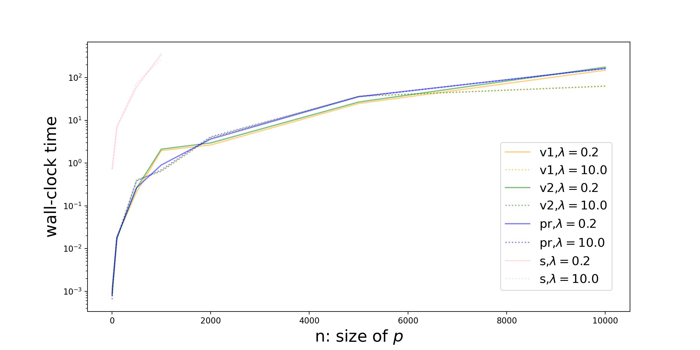
In this section, we present the wall clock time comparison between our method Algorithms 1, 2, the Frank-wolf algorithm proposed in [10], and its Sinkhorn version [40, 10]. Note that these two baselines solve a mass constraint version of the PGW problem, which we refer to as the “primal-PGW” problem. The proposed PGW formulation in this paper can be regarded as an “Lagragian formulation” of primal-PGW formulation to the PGW problem defined in (12). In this paper, we call these two baselines as “primal-PGW algorithm” and “Sinkhorn PGW algorithm”.

The data is generated as follows: let $\mu=\text{Unif}([0,2]^{2})$ and $\nu=\text{Unif}([0,2]^{3})$, we select i.i.d. samples $\{x_{i}\sim\mu\}_{i=1}^{n},\{y_{j}\sim\nu\}_{j=1}^{m}$, where $n$ is selected from $[10,50,100,150,...,10000]$ and $m=n+100$, $\mathrm{p}=1_{n}/m,\mathrm{q}=1_{m}/m$. For each $n$, we set $\lambda=0.2,1.0,10.0$. The mass constraint parameter for the algorithm in [10], and Sinkhorn is computed by the mass of the transportation plan obtained by Algorithm 1 or 2. The runtime results are shown in Figure 1.

Regarding the acceleration technique, for the POT problem in step 1, our algorithms and the primal-PGW algorithm apply the linear programming solver provided by Python OT package [22], which is written in C++. The Sinkhorn algorithm from Python OT does not have an acceleration technique. Thus, we only test its wall-clock time for $n\leq 2000$. The data type is 64-bit float number. The experiment is conducted on a computational machine with AMD 64-core Processors clocking 3720 MHZ and 4 NVIDA RTX A6000 49 GB GPUs.

From this Figure 1, we can observe the Algorithms 1, 2 and primal-PGW algorithm have a similar order of time complexity. However, using the column/row-reduction technique for the POT computation discussed in previous sections, and the fact the convergence behaviors of Algorithms 1 and 2 are similar to the primal-PGW algorithm, we observe that the proposed algorithms 1, 2 admits a slightly faster speed than primal-PGW solver.

5.2 Shape matching problem between 2D and 3D spaces

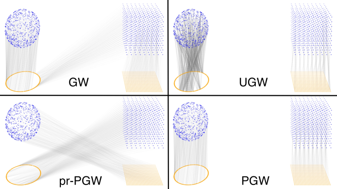
In this section, we consider a simple shape-matching problem. Suppose sets $SQ_{2}=\{s^{2}_{i}\in\mathbb{R}^{2}\}_{i=1}^{n},SQ_{3}=\{s^{3}_{i}\in\mathbb{R}^{3}\}_{i=1}^{n}$ are sampled from a 2D square $[-1,1]^{2}$ and a 3D cube $[-1,1]^{3}$, respectively. Similarly, $SP_{2}=\{c^{2}_{i}\in\mathbb{R}^{2}\}_{i=1}^{n},SP_{3}=\{c^{3}_{i}\in\mathbb{R}^{3}\}_{i=1}^{n}$ are sampled from a 2D circle $\{s^{2}+[5,0]:\|s^{2}\|^{2}=1\}$ and a 3D sphere $\{s^{3}+[5,0,0]:\|s^{3}\|=1\}$. Given $a,b>0$ with $a+b=1$, we use $aS_{2}+bC_{2}$ to denote the mixture probability distribution supported on $SQ_{2}\cup SP_{2}$. In particular, the probability mass of each point in $SQ_{2}$ is $a\frac{1}{n}$ and the mass of each points in $SP_{2}$ is $b\frac{1}{n}$. Similarly, we define $aS_{3}+bC_{3}$.

Given distributions $0.3S_{2}+0.7C_{2}$ and $0.5S_{3}+0.5C_{3}$, we visualize the matching between them via balanced Gromov-Wasserstein (GW), Unbalanced Gromov-Wasserstein (UGW), the Primal partial Gromov-Wasserstein approach (primal-PGW), and the partial Gromov-Wasserstein framework proposed in this paper (PGW).

For GW and UGW, the initial guess $\gamma^{(1)}$ is set to be $\mathrm{p}\mathrm{q}^{T}$, for primal-PGW, $\gamma^{(1)}$ is $\frac{m\mathrm{p}\mathrm{q}^{T}}{|\mathrm{p}||\mathrm{q}|}$, and for PGW, $\frac{\mathrm{p}\mathrm{q}^{T}}{\max(|\mathrm{p}|,|\mathrm{q}|)}$. The optimal correspondences for each method are visualized in Figure 2. We observe that UGW, primal-PGW, and PGW induce more natural correspondences in this unbalanced setting. Note that GW matches the same 3D shape (SQ3) to the two different 2D shapes, as it requires mass preservation.

Regarding the wall-clock time, the size of two distributions is set to be 1200, denoted as $n$. GW requires 4-6 seconds, primal-PGW requires 70-80 seconds, UGW requires 38-46 seconds and PGW requires 26-30 seconds.

The maximum iteration for OT solver in GW, PGW, primal-PGW is set to be $300n$. The maximum iteration in Sinkhorn step in UGW is set to be 1000. The data type for GW, PGW, primal-PGW is 64-bit float number, the data type for UGW is 32-bit float number.

Figure 2: Shape matching results via GW, Primal-PGW, UGW, and PGW. In each subplot, the top two shapes are $SQ3,SP3$, and the bottom two shapes are $SQ2,SP2$. We visualize correspondences if the transported mass is greater than a suitable threshold.

5.3 Positive unlabeled learning problem

Dataset	Init	Pr-PGW	UGW	PGW
M $\to$ M	POT, 100%	100%	95%	100%
M $\to$ M	FLB-U, 75%	96%	95%	96%
M $\to$ M	FLB-P, 75%	99%	95%	99%
M $\to$ EM	FLB-U, 78%	94%	95%	94%
M $\to$ EM	FLB-P, 78%	94%	95%	94%
EM $\to$ M	FLB-U, 75%	97%	96%	97%
EM $\to$ M	FLB-P, 75%	97%	96%	97%
EM $\to$ EM	POT, 100%	100%	95%	100%
EM $\to$ EM	FLB-U, 78%	94%	95%	94%
EM $\to$ EM	FLB-P, 78%	95%	95%	95%

Table 1: Accuracy comparison of the primal-PGW, UGW, and the proposed PGW method on PU learning. “Init” denotes the initialization method and initial accuracy. ‘M’ denotes MNIST, and ‘EM’ denotes EMNIST.

Problem Setup. Positive unlabeled (PU) learning [4, 18, 29] is a semi-supervised binary classification problem for which the training set only contains positive samples. In particular, suppose there exists a fixed unknown overall distribution over triples $(x,o,l)$, where $x$ is data, $l\in\{0,1\}$ is the label of $x$, $o\in\{0,1\}$ where $o=1$, $o=0$ denote that $l$ is observed or not, respectively. In the PU task, the assumption is that only positive samples’ labels can be observed, i.e., $\text{Prob}(o=1|x,l=0)=0.$ Consider training labeled data $X^{p}=\{(x_{i}^{p},l)\}_{i=1}^{n}\subset\{x:o=1\}$ and testing data $X^{u}=\{x_{j}^{u}\}_{j=1}^{m}\subset\{x:o=0\}$, where $x^{p}_{i}\in\mathbb{R}^{d_{1}},x^{u}_{j}\in\mathbb{R}^{d_{2}}$. In the classical PU learning setting, $d_{2}=d_{1}$. However, in [44] this assumption is relaxed. The goal is to leverage $X^{p}$ to design a classifier $\hat{l}:x^{u}\to\{0,1\}$ to predict $l(x^{u})$ for all $x^{u}\in X^{u}$.

Following [18, 10, 44], in this experiment, we assume that the “select completely at random” (SCAR) assumption holds: $\text{Prob}(o=1|x,l=1)=\text{Prob}(o=1|l=1)$. In addition, we use $\pi=\text{Prob}(l=1)\in[0,1]$ to denote the ratio of positive samples in testing set. Following the PU learning setting in [29, 28, 10, 44], we assume $\pi$ is known. In all the PU learning experiments, we fix $\pi=0.2$.

Our method. Similar to [10] our method is designed as follows: We set $\mathrm{p}\in\mathbb{R}^{n},\mathrm{q}\in\mathbb{R}^{m}$ as $p_{i}=\frac{\pi}{n},i\in[1:n];\quad q_{j}=\frac{1}{m},j\in[1:m].$ Let $\mathbb{X}^{p}=(X^{p},\|\cdot\|_{d_{1}},\sum_{i=1}^{n}p_{i}\delta_{x_{i}}),\mathbb{X}^{u}=(X^{u},\|\cdot\|_{d_{2}},\sum_{j=1}^{n}q_{j}\delta_{y_{j}})$. We solve the partial GW problem $PGW_{\lambda}(\mathbb{X}^{p},\mathbb{X}^{u})$ and suppose $\gamma$ is a solution. Let $\gamma_{2}=\gamma^{T}1_{n}$. The classifier $\hat{l}$ is defined by the indicator function.

$$\hat{l}_{\gamma}(x^{u})=\mathbbm{1}_{\{x^{u}:\,\gamma_{2}(x^{u})\geq\mathrm{quantile}\}},$$ (35)

where $\mathrm{quantile}$ is the quantile value of $\gamma_{2}$ according to $1-\pi$.

Regarding the initial guess $\gamma^{(1)}$, [10] proposed a POT-based approach when $X$ and $Y$ are sampled from the same domain, i.e., $d_{1}=d_{2}$, which we refer to as “POT initialization.” The initial guess $\gamma^{(1)}$ is given by the following partial OT variant problem:

$$\gamma^{(1)}=\arg\min_{\gamma\in\Gamma_{PU,\pi}(\mathrm{p},\mathrm{q})}\langle L(X,Y),\gamma\rangle_{F},$$ (36)

where $L(X,Y)\in\mathbb{R}^{n\times m},\,(L(X,Y))_{ij}=\|x_{i}-y_{j}\|^{2}$ and

$$\Gamma_{PU,\pi}(\mathrm{p},\mathrm{q}):=\{\gamma\in\mathbb{R}_{+}^{n\times m}:(\gamma^{T}1_{n})_{j}\in\{q_{j},0\},\forall j;$$

$$\qquad\quad\quad\quad\quad\quad\gamma 1_{m}\leq\mathrm{p},|\gamma|=\pi\}.$$ (37)

The above problem can be solved by a Lasso ($L^{1}$ norm) regularized OT solver.

When $X,Y$ are sampled from different spaces, that is, $d_{1}\neq d_{2}$, the above technique (36) is not well-defined. Inspired by [37, 44], we propose the following “first lower bound-partial OT” (FLB-POT) initialization:

$$\gamma^{(1)}=\arg\min_{\gamma\in\Gamma_{\leq}(\mathrm{p},\mathrm{q})} \int_{X\times Y}|s_{X,2}(x)-s_{Y,2}(y)|^{2}d\gamma(x,y)$$

$$\quad+\lambda(|\mathrm{p}-\gamma_{1}|+|\mathrm{q}-\gamma_{2}|),$$ (38)

where $s_{X,2}(x)=\int_{X}|x-x^{\prime}|^{2}d\mu(x)$ and $s_{Y,2}$ is defined similarly. The above formula is analog to Eq. (7) in [44], which is designed for the unbalanced GW setting. To distinguish them, in this paper we call the Eq. (7) in [44] as “FLB-UOT initilization”.

Dataset. The datasets include MNIST, EMNIST, and the following three domains of Caltech Office: Amazon (A), Webcam (W), and DSLR (D) [42]. For each domain, we select the SURF features [42] and DECAF features [17]. For MNIST and EMNIST, we train an auto-encoder respectively and the embedding space dimension is $4$ and $6$ respectively.

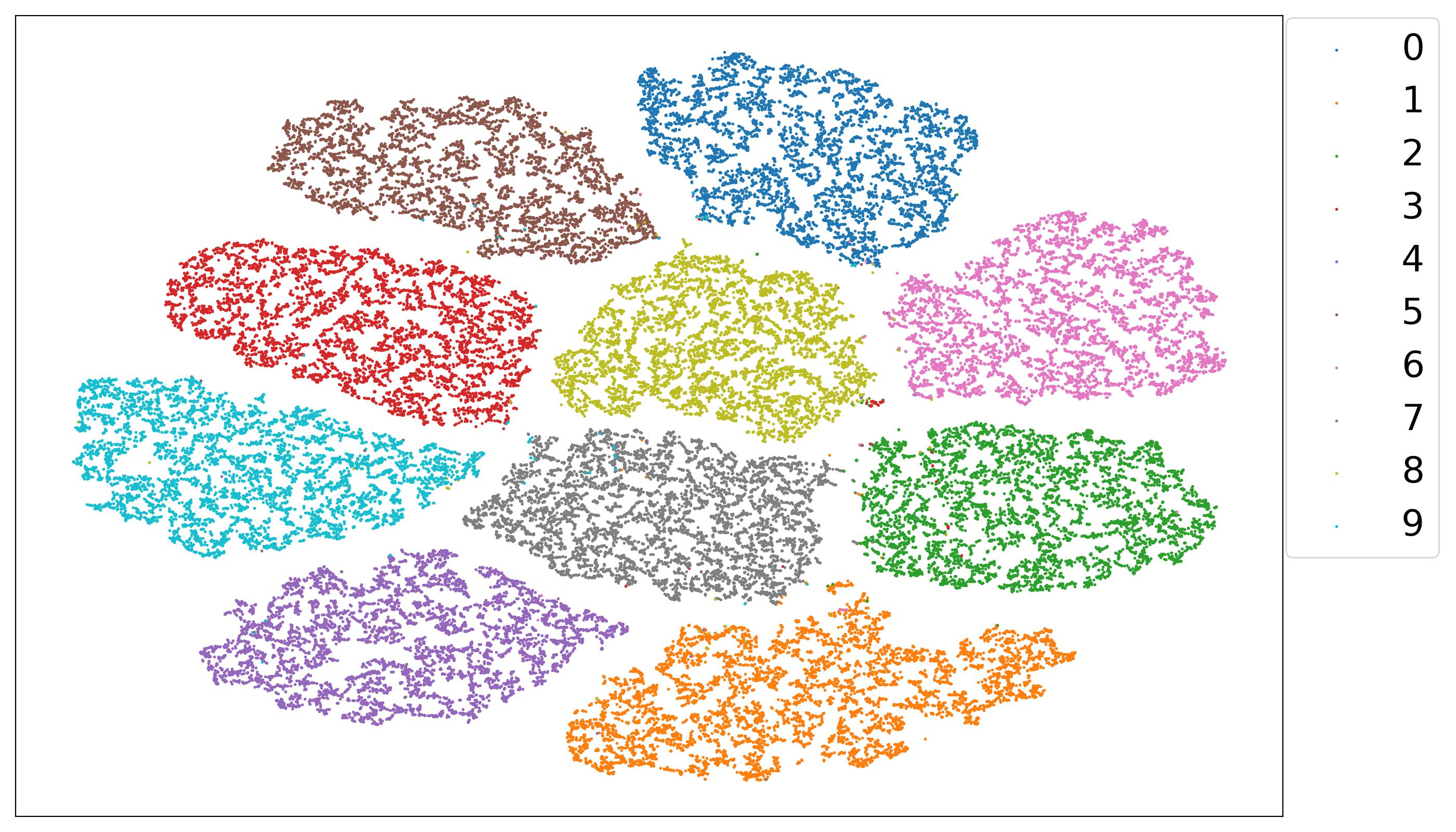
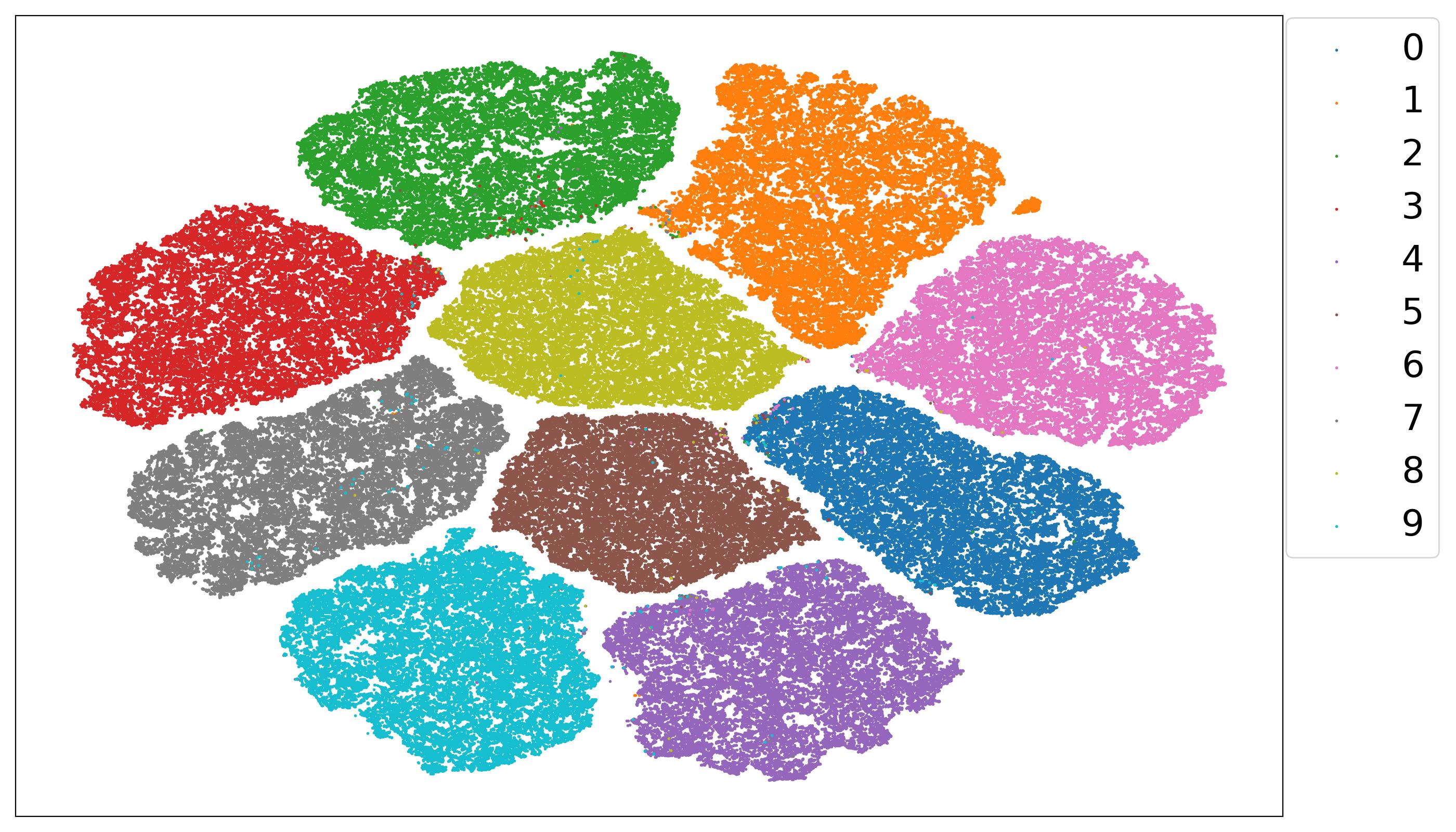
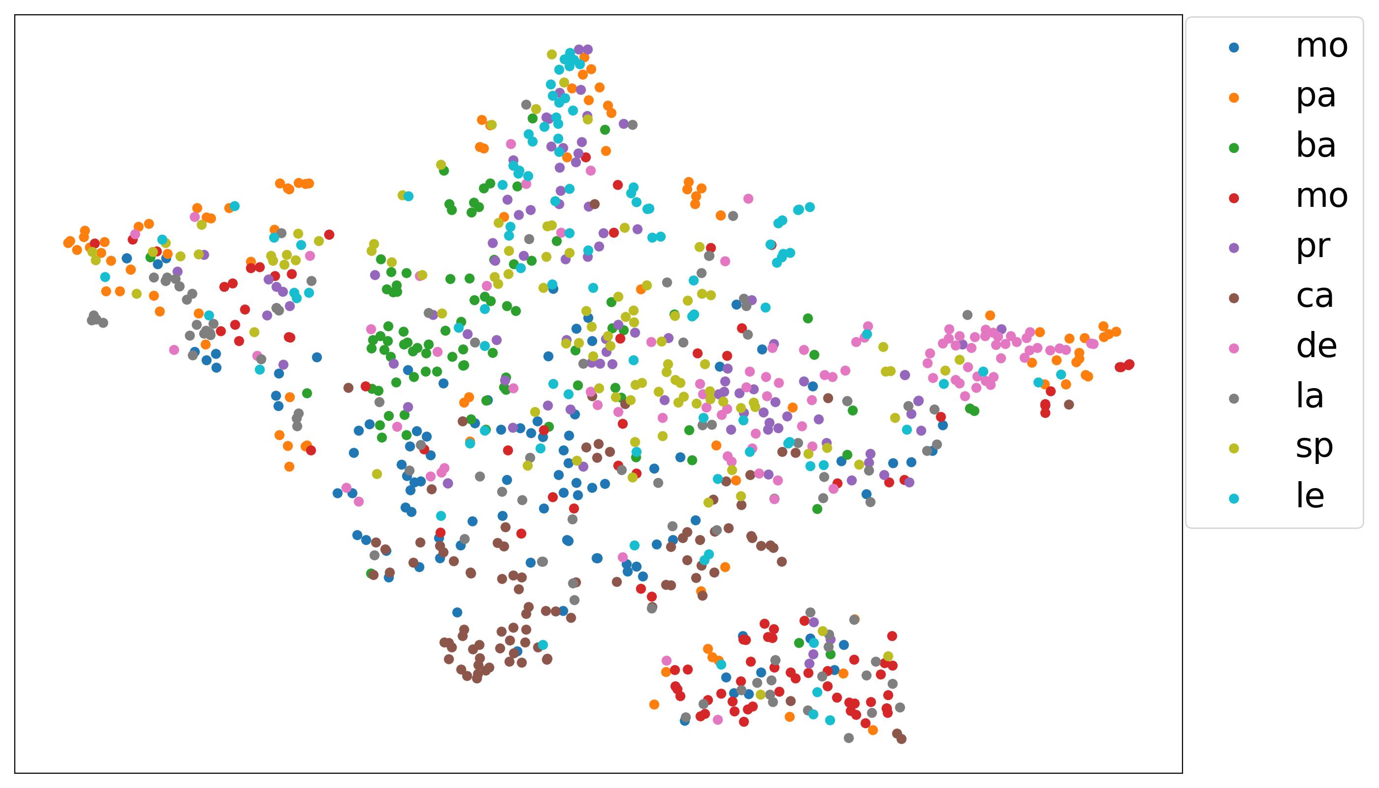
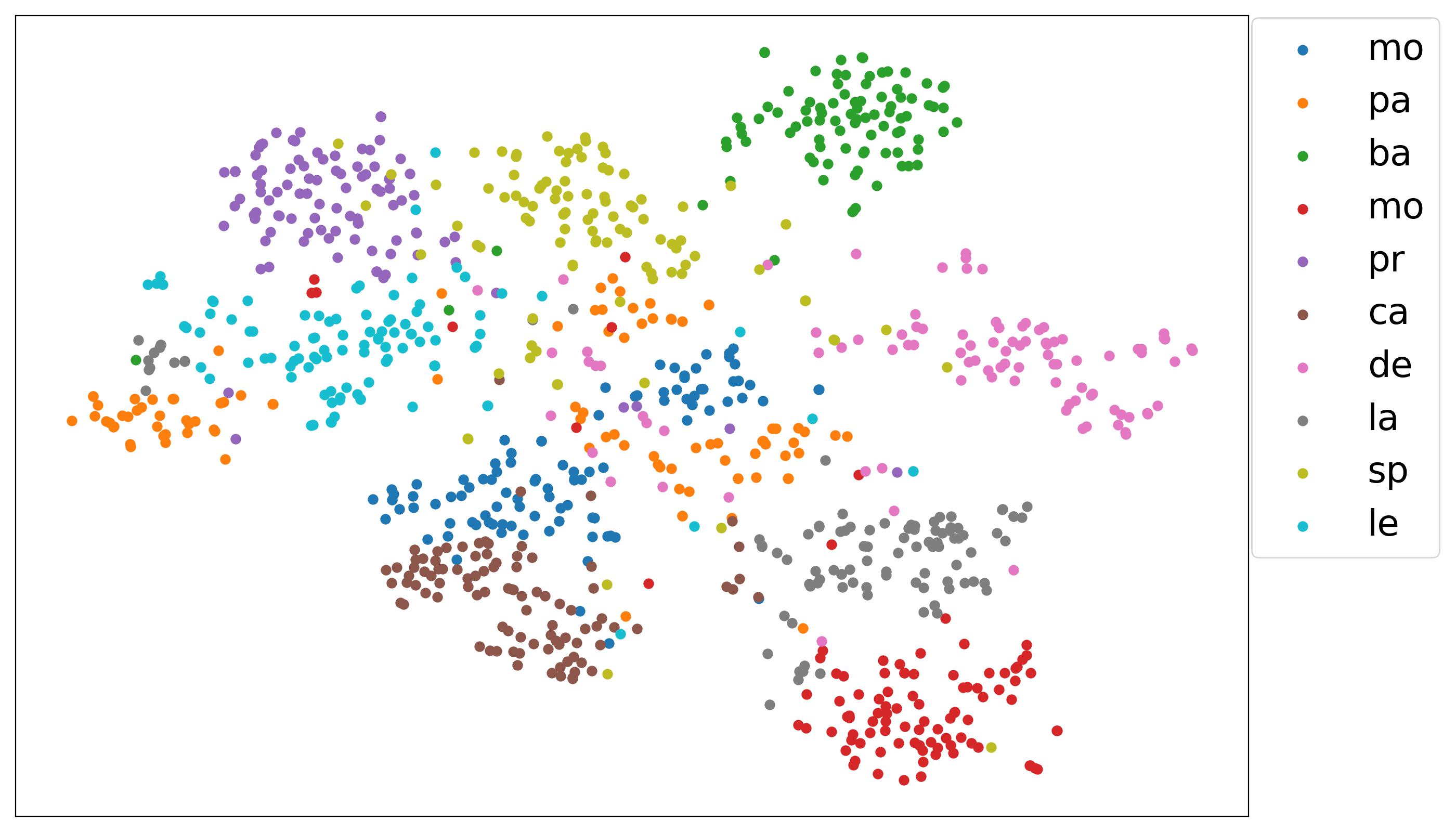
Performance. In the Table 1, we present the accuracy comparison between PGW, UGW, and our method on MNIST, EMNIST datasets. The PU learning results on the Caltech Office dataset are included in the appendix. Regarding the wall-clock time, typically Primal-PGW and PGW require 1-35 seconds, UGW requires 100-160 seconds. See the Appendix for the complete accuracy table on all datasets, the visualization of all datasets, and the wall-clock time table.

6 Summary

In this paper, we extend McCann’s technique to the Partial Gromov-Wasserstein (PGW) setting and introduce two Frank-Wolfe algorithms for the PGW problem. As a byproduct, we provide pertinent theoretical results, including the relation between PGW and GW, the metric properties of PGW, and the convergence behavior of our proposed solvers. Furthermore, we demonstrate the efficacy of the PGW solver in solving shape-matching problems and PU learning tasks.

7 Acknowledgment

This work was partially supported by the NSF CAREER award under Grant No. 2339898.

Appendix A Notation and abbreviations

• OT: Optimal Transport.

• POT: Partial Optimal Transport.

• GW: Gromov-Wasserstein.

• PGW: Partial Gromov-Wasserstein minimization problem.

• FW: Frank-Wolfe.

• $S\subset\mathbb{R}^{d_{1}},X\subset\mathbb{R}^{d_{2}},Y\subset\mathbb{R}^{d_{3}}$: subsets in Euclidean spaces.

• $\|\cdot\|$: Euclidean norm.

• $X^{2}=X\times X$.

• $\mathcal{M}_{+}(S)$: set of all positive (non-negative) Randon (finite) measures defined on $S$.

• $\mathcal{P}_{2}(S)$: set of all probability measures defined on $S$, whose second moment is finite.

• $\mathbb{R}_{+}$: set of all non-negative real numbers.

• $\mathbb{R}^{n\times m}$: set of all $n\times m$ matrices with real coefficients.

• $\mathbb{R}^{n\times m}_{+}$ (resp. $\mathbb{R}^{n}_{+}$): set of all $n\times m$ matrices (resp., $n$-vectors) with non-negative coefficients.

• $\mathbb{R}^{n\times m\times n\times m}$: set of all $n\times m\times n\times m$ tensors with real coefficients.

• $1_{n},1_{n\times m},1_{n\times m\times n\times m}$: vector, matrix, and tensor of all ones.

• $\mathbbm{1}_{E}$: characteristic function of a measurable set $E$

  $$\mathbbm{1}_{E}(z)=\begin{cases}1&\text{ if }z\in E,\\ 0&\text{ otherwise.}\end{cases}$$

• $\mathbb{S},\mathbb{X},\mathbb{Y}$: metric measure spaces (mm-spaces): $\mathbb{S}=(S,d_{S},\sigma),\,\mathbb{X}=(X,d_{X},\mu),\,\mathbb{Y}=(Y,d_{Y},\nu).$

• $C^{X}$: given a discrete mm-space $\mathbb{X}=(X,d_{X},\mu)$, where $X=\{x_{1},\dots,x_{n}\}$, the symmetric matrix $C^{X}\in\mathbb{R}^{n\times n}$ is defined as $C^{X}_{i,i^{\prime}}=d_{X}(x_{i},x_{i}^{\prime})$.

• $\mu^{\otimes 2}$: product measure $\mu\otimes\mu$.

• $T_{\#}\sigma$: $T$ is a measurable function and $\sigma$ is a measure on $X$. $T_{\#}\sigma$ is the push-forward measure of $\sigma$, i.e., its is the measure on $Y$ such that for all Borel set $A\subset Y$, $T_{\#}\sigma(A)=\sigma(T^{-1}(A))$.

• $\gamma,\gamma_{1},\gamma_{2}$: $\gamma$ is a joint measure defined for example in $X\times Y$; $\gamma_{1},\gamma_{2}$ are the first and second marginals of $\gamma$, respectively. In the discrete setting, they are viewed as matrix and vectors, i.e., $\gamma\in\mathbb{R}_{+}^{n\times m}$, and $\gamma_{1}=\gamma 1_{m}\in\mathbb{R}_{+}^{n}$, $\gamma_{2}=\gamma^{T}1_{n}\in\mathbb{R}_{+}^{m}$.

• $\Gamma(\mu,\nu)$, where $\mu\in\mathcal{P}_{2}(X),\nu\in\mathcal{P}_{2}(Y)$ (where $X,Y$ may not necessarily be the same set): it is the set of all the couplings (transportation plans) between $\mu$ and $\nu$, i.e., $\Gamma(\mu,\nu):=\{\gamma\in\mathcal{P}_{2}(X\times Y):\,\gamma_{1}=\mu,\gamma_{2}=\nu\}.$

• $\Gamma(\mathrm{p},\mathrm{q})$: it is the set of all the couplings between the discrete probability measures $\mu=\sum_{i=1}^{n}p_{i}\delta_{x_{i}}$ and $\nu=\sum_{j=1}^{m}y_{j}\delta_{y_{j}}$ with weight vectors

  $$\mathrm{p}=[p_{1},\dots,p_{n}]^{T}\qquad\text{ and }\qquad\mathrm{q}=[q_{1},\dots,q_{n}]^{T}.$$ (39)

  That is, $\Gamma(\mathrm{p},\mathrm{q})$ coincides with $\Gamma(\mu,\nu)$, but it is viewed as a subset of $n\times m$ matrices defined in (19).

• $p,q$: real numbers $1\leq p,q<\infty$.

• $\mathrm{p},\mathrm{q}$: vectors of weights as in (39).

• $\mathrm{p}=[p_{1},\dots,p_{n}]\leq\mathrm{p}^{\prime}=[p^{\prime}_{1},\dots,p^{\prime}_{n}]$ if $p_{j}\leq p_{j}^{\prime}$ for all $1\leq j\leq n$.

• $|\mathrm{p}|=\sum_{i=1}^{n}p_{i}$ for $\mathrm{p}=[p_{1}\dots,p_{n}]$.

• $c(x,y):X\times Y\to\mathbb{R}_{+}$ denotes the cost function used for classical and partial optimal transport problems. lower-semi continuous function.

• $OT(\mu,\nu)$: it is the classical optimal transport (OT) problem between the probability measures $\mu$ and $\nu$ defined in (1).

• $W_{p}(\mu,\nu)$: it is the $p$-Wasserstein distance between the probability measures $\mu$ and $\nu$ defined in (2), for $1\leq p<\infty$.

• The Partial Optimal Transport (OPT) problem is defined in (3) or, equivalently, in (4).

• $|\mu|$: total variation norm of the positive Randon (finite) measure $\mu$ defined on a measurable space $X$, i.e., $|\mu|=\mu(X)$.

• $\mu\leq\sigma$: denotes that for all Borel set $B\subseteq X$ we have that the measures $\mu,\sigma\in\mathcal{M}_{+}(X)$ satisfy $\mu(B)\leq\sigma(B)$.

• $\Gamma_{\leq}(\mu,\nu)$, where $\mu\in\mathcal{M}_{+}(X),\nu\in\mathcal{M}_{+}(Y)$: it is the set of all “partial transportation plans”

  $$\Gamma_{\leq}(\mu,\nu):=\{\gamma\in\mathcal{M}_{+}(X\times Y):\,\gamma_{1}\leq\mu,\gamma_{2}\leq\nu\}.$$

• $\Gamma_{\leq}(\mathrm{p},\mathrm{q})$: it is the set of all the “partial transportation plans” between the discrete probability measures $\mu=\sum_{i=1}^{n}p_{i}\delta_{x_{i}}$ and $\nu=\sum_{j=1}^{m}y_{j}\delta_{y_{j}}$ with weight vectors $\mathrm{p}=[p_{1},\dots,p_{n}]$ and $\mathrm{q}=[q_{1},\dots,q_{n}]$. That is, $\Gamma_{\leq}(\mathrm{p},\mathrm{q})$ coincides with $\Gamma_{\leq}(\mu,\nu)$, but it is viewed as a subset of $n\times m$ matrices defined in (20).

• $\lambda>0$: positive real number.

• $\hat{\infty}$: auxiliary point.

• $\hat{X}=X\cup\{\hat{\infty}\}$.

• $\hat{\mu},\hat{\nu}$: given in (5).

• $\hat{\mathrm{p}},\hat{\mathrm{q}}$: given in (24).

• $\hat{\gamma}$: given in (8).

• $\hat{c}(\cdot,\cdot):\hat{X}\times\hat{Y}\to\mathbb{R}_{+}$: cost as in (6).

• $L:\mathbb{R}\times\mathbb{R}\to\mathbb{R}$: cost function for the GW problems.

• $D:\mathbb{R}\times\mathbb{R}\to\mathbb{R}$: generic distance on $\mathbb{R}$ used for GW problems.

• $GW_{q}^{L}(\cdot,\cdot)$: GW optimization problem given in (9).

• $GW_{q}^{p}(\cdot,\cdot)$: GW optimization problem given in (9) when $L(\cdot,\cdot)=D^{p}(\cdot,\cdot)$.

• $GW_{g}(\cdot,\cdot)$: generalized GW problem given in (52).

• $\widehat{GW}$: GW-variant problem given in (15) for the general case, and in (26) for the discrete setting.

• $\hat{L}$: cost given in (14) for the GW-variant problem.

• $\hat{d}:\hat{X}\times\hat{X}\to\mathbb{R}_{+}\cup\{\infty\}$: “generalized” metric given in (13) for $\hat{X}$.

• $\mathcal{G}_{q}$: subset of mm-spaces given in (10).

• $\mathbb{X}\sim\mathbb{Y}$: equivalence relation in $\mathcal{G}_{q}$, where given $\mathbb{X},\mathbb{Y}\in\mathcal{G}_{q}$, we define $\mathbb{X}\sim\mathbb{Y}$ if and only if $GW_{q}^{p}(\mathbb{X},\mathbb{Y})=0$.

• $PGW_{\lambda,q}^{L}(\cdot,\cdot)$: partial GW optimization problem given in (11) or, equivalently, in (12).

• $PGW_{\lambda,q}(\cdot,\cdot)$: partial GW problem $PGW_{\lambda,q}^{L}(\cdot,\cdot)$ for which $L(r_{1},r_{2})=D(r_{1},r_{2})^{p}$ for a metric $D$ in $\mathbb{R}$, and $1\leq p<\infty$.Typically $D(r_{1},r_{2})=|r_{1}-r_{2}|$, and $p=2$. It is explicitly given in (17).

• $PGW_{\lambda}(\cdot,\cdot)$: discrete partial GW problem given in (23).

• $\mathcal{L}$: functional for the optimization problem $PGW_{\lambda}(\cdot,\cdot)$.

• $M$, $\tilde{M}$, and $\hat{M}$: see (21), (22), and (25), respectively.

• $\langle\cdot,\cdot\rangle_{F}$: Frobenius inner product for matrices, i.e., $\langle A,B\rangle_{F}=\mathrm{trace}(A^{T}B)=\sum_{i,j}^{n,m}A_{i,j}B_{i,j}$ for all $A,B\in\mathbb{R}^{n\times m}$.

• $M\circ\gamma$: product between the tensor $M$ and the matrix $\gamma$.

• $\nabla$: gradient.

• $[1:n]=\{1,\dots,n\}$.

• $\alpha$: step size based on the line search method.

• $\gamma^{(1)}$: initialization of the algorithm.

• $\gamma^{(k)}$, $\gamma^{(k)^{\prime}}$: previous and new transportation plans before and after step 1 in the $k-$th iteration of version 1 of our proposed FW algorithm.

• $\hat{\gamma}^{(k)}$, $\hat{\gamma}^{(k)^{\prime}}$: previous and new transportation plans before and after step 1 in the $k-$th iteration of version 2 of our proposed FW algorithm.

• $G=2\tilde{M}\circ\gamma$, $\hat{G}=2\hat{M}\circ\hat{\gamma}$: Gradient of the objective function in version 1 and version 2, respectively, of our proposed FW algorithm for solving the discrete version of partial GW problem.

• $(\delta\gamma,a,b)$ and $(\delta\hat{\gamma},a,b)$: given in (31) and (34) for versions 1 and 2 of the algorithm, respectively.

• $C^{1}$-function: continuous and with continuous derivatives.

• $\Gamma_{PU,\pi}(\mathrm{p},\mathrm{q})$: defined in (5.3)

Appendix B Proof of Proposition 3.1

For the first statement, the idea of the proof is inspired by the proof of Proposition 1 in [41].

The goal is to verify that

$$PGW_{\lambda,q}^{L} (\mathbb{X},\mathbb{Y}):=\underbrace{\inf_{\gamma\in\mathcal{M}_{+}(X,Y)}\int_{(X\times Y)^{2}}L(d_{X}^{q}(x,x^{\prime}),d_{Y}^{q}(y,y^{\prime}))d\gamma(x,y)d\gamma(x^{\prime},y^{\prime})}_{\text{transport GW cost}}+\underbrace{\lambda\left(|\mu^{\otimes 2}-\gamma_{1}^{\otimes 2}|+|\nu^{\otimes 2}-\gamma_{2}^{\otimes 2}|\right)}_{\text{mass penalty}}$$

$$={\inf_{\gamma\in\Gamma_{\leq}(\mu,\nu)}\int_{(X\times Y)^{2}}L(d_{X}^{q}(x,x^{\prime}),d_{Y}^{q}(y,y^{\prime}))d\gamma(x,y)d\gamma(x^{\prime},y^{\prime})}+{\lambda\left(|\mu^{\otimes 2}-\gamma_{1}^{\otimes 2}|+|\nu^{\otimes 2}-\gamma_{2}^{\otimes 2}|\right)}.$$ (40)

Given one $\gamma\in\mathcal{M}_{+}(X\times Y)$ such that $\gamma_{1}\leq\mu$ does not hold. Then we can write the Lebesgue decomposition of $\gamma_{1}$ with respect to $\mu$:

$$\gamma_{1}=f\mu+\mu^{\perp},$$

where $f\geq 0$ is the Radon-Nikodym derivative of $\gamma_{1}$ with respect to $\mu$, and $\mu^{\perp},\mu$ are mutually singular, that is, there exist measurable sets $A,B$ such that $A\cap B=\emptyset$, $X=A\cup B$ and $\mu^{\perp}(A)=0,\mu(B)=0$. Without loss of generality, we can assume that the support of $f$ lies on $A$, since

$$\gamma_{1}(E)=\int_{E\cap A}f(x)\,d\mu(x)+\mu^{\perp}(E\cap B)\qquad\forall E\subseteq X\text{ measurable}.$$

Define $A_{1}=\{x\in A:\,f(x)>1\},A_{2}=\{x\in A:\,f(x)\leq 1\}$ (both are measurable, since $f$ is measurable), and define $\bar{\mu}=\min\{f,1\}\mu$. Then,

$$\bar{\mu}\leq\mu\qquad\text{ and }\qquad\bar{\mu}\leq f\mu\leq f\mu+\mu^{\perp}=\gamma_{1}.$$

There exists a $\bar{\gamma}\in\mathcal{M}_{+}(X\times Y)$ such that $\bar{\gamma}_{1}=\bar{\mu},\bar{\gamma}\leq\gamma$, and $\bar{\gamma}_{2}\leq\gamma_{2}$. Indeed, we can construct $\bar{\gamma}$ in the following way: First, let $\{\gamma^{x}\}_{x\in X}$ be the set of conditional measures (disintegration) such that for every measurable (test) function $\psi:X\times Y\to\mathbb{R}$ we have

$$\int\psi(x,y)\,d\gamma(x,y)=\int_{X}\int_{Y}\psi(x,y)\,d\gamma^{x}(y)\,d\gamma_{1}(x).$$

Then, define $\bar{\gamma}$ as

$$\bar{\gamma}(U):=\int_{X}\int_{Y}\mathbbm{1}_{U}(x,y)\,d\gamma^{x}(y)\,d\bar{\mu}(x)\qquad\forall U\subseteq X\times Y\text{ Borel}.$$

Then, $\bar{\gamma}$ verifies that $\bar{\gamma}_{1}=\bar{\mu}$, and since $\bar{\mu}\leq\gamma_{1}$, we also have that $\bar{\gamma}\leq\gamma$, which implies $\bar{\gamma}_{2}\leq\gamma_{2}$.

Since $|\gamma_{1}|=|\gamma_{2}|$ and $|\bar{\gamma}_{1}|=|\bar{\gamma}_{2}|$, then we have $|\gamma_{1}^{\otimes 2}-\bar{\gamma}_{1}^{\otimes 2}|=|\gamma_{2}^{\otimes 2}-\bar{\gamma}_{2}^{\otimes 2}|$.

We claim that

$$|\mu^{\otimes 2}-\gamma_{1}^{\otimes 2}|\geq|\mu^{\otimes 2}-\bar{\gamma}_{1}^{\otimes 2}|+|\gamma_{1}^{\otimes 2}-\bar{\gamma}_{1}^{\otimes 2}|.$$ (41)

• Left-hand side of (41): Since $\{A,B\}$ is a partition of $X$, we first spit the left-hand side of (41) as

  $$|\mu^{\otimes 2}-\gamma_{1}^{\otimes 2}|=\underbrace{|\mu^{\otimes 2}-\gamma_{1}^{\otimes 2}|(A\times A)}_{(I)}+\underbrace{|\mu^{\otimes 2}-\gamma_{1}^{\otimes 2}|(A\times B)+|\mu^{\otimes 2}-\gamma_{1}^{\otimes 2}|(B\times A)}_{(II)}+\underbrace{|\mu^{\otimes 2}-\gamma_{1}^{\otimes 2}|(B\times B)}_{(III)}.$$

  Then we have

  $$(III)=|\mu^{\otimes 2}-\gamma_{1}^{\otimes 2}|(B\times B)=\mu^{\perp}\otimes\mu^{\perp}(B\times B)=|\mu^{\perp}|^{2},$$

  $$(II)=|\mu^{\otimes 2}-\gamma_{1}^{\otimes 2}|(A\times B)+|\mu^{\otimes 2}-\gamma_{1}^{\otimes 2}|(B\times A) =2|\mu^{\perp}|\cdot(|\mu-\gamma_{1}|(A)).$$

  Since $\gamma_{1}=f\mu$ in $A$, then $\bar{\gamma}_{1}=\gamma_{1}$ in $A_{2}$ and $\bar{\gamma}_{1}=\mu$ in $A_{1}$, so we have

  $$|\mu-\gamma_{1}|(A) =|\mu-\gamma_{1}|(A_{1})+|\mu-\gamma_{1}|(A_{2})=(\gamma_{1}-\bar{\gamma}_{1})(A_{1})+(\mu-\bar{\gamma}_{1})(A_{2})=|\gamma_{1}-\bar{\gamma}_{1}|(A)+|\mu-\bar{\gamma}_{1}|(A).$$

  Thus,

  $$(II) =2|\mu^{\perp}|\cdot(|\gamma_{1}-\bar{\gamma}_{1}|(A)+|\mu-\bar{\gamma}_{1}|(A)),$$

  and we also get that

  $$(I) =|\mu^{\otimes 2}-\gamma_{1}^{\otimes 2}|(A\times A)$$

  $$=|\mu^{\otimes 2}-\gamma_{1}^{\otimes 2}|({A_{1}\times A_{1}})+|\mu^{\otimes 2}-\gamma_{1}^{\otimes 2}|(A_{2}\times A_{2})+|\mu^{\otimes 2}-\gamma_{1}^{\otimes 2}|(A_{1}\times A_{2})+|\mu^{\otimes 2}-\gamma_{1}^{\otimes 2}|(A_{2}\times A_{1})$$

  $$=(\gamma_{1}^{\otimes 2}-\bar{\gamma}_{1}^{\otimes 2})({A_{1}\times A_{1}})+(\mu^{\otimes 2}-\bar{\gamma}_{1}^{\otimes 2})(A_{2}\times A_{2})+$$

  $$\qquad+|\bar{\gamma}_{1}\otimes\mu-\gamma_{1}\otimes\bar{\gamma}_{1}|(A_{1}\times A_{2})+|\mu\otimes\bar{\gamma}_{1}-\bar{\gamma}_{1}\otimes\gamma_{1}|(A_{2}\times A_{1})$$

  $$=(\gamma_{1}^{\otimes 2}-\bar{\gamma}_{1}^{\otimes 2})({A_{1}\times A_{1}})+(\mu^{\otimes 2}-\bar{\gamma}_{1}^{\otimes 2})(A_{2}\times A_{2})+2|\bar{\gamma}_{1}-\gamma_{1}|(A_{1})\cdot|\mu-\bar{\gamma}_{1}|(A_{2})$$

  $$=|\gamma_{1}^{\otimes 2}-\bar{\gamma}_{1}^{\otimes 2}|({A\times A})+|\mu^{\otimes 2}-\bar{\gamma}_{1}^{\otimes 2}|(A\times A)+\underbrace{2|\bar{\gamma}_{1}-\gamma_{1}|(A_{1})\cdot|\mu-\bar{\gamma}_{1}|(A_{2})}_{\geq 0}.$$

• Right-hand side of (41): First notice that

  $$|\gamma_{1}-\bar{\gamma}_{1}|(B)=(\gamma_{1}-\bar{\gamma}_{1})(B)\leq\gamma_{1}(B)=|\mu^{\perp}|,$$ (42)

  and since $\bar{\gamma}_{1}\leq\mu$ and $\mu(B)=0$, we have

  $$|\mu-\bar{\gamma}_{1}|(B)=0.$$ (43)

  Then,

  $$|\mu^{\otimes 2}-\bar{\gamma}_{1}^{\otimes 2}|+|\gamma_{1}^{\otimes 2}-\bar{\gamma}_{1}^{\otimes 2}|=$$

  $$=|\mu^{\otimes 2}-\bar{\gamma}_{1}^{\otimes 2}|(A\times A)+|\gamma_{1}^{\otimes 2}-\bar{\gamma}_{1}^{\otimes 2}|(A\times A)+|\mu^{\otimes 2}-\bar{\gamma}_{1}^{\otimes 2}|(B\times B)+|\gamma_{1}^{\otimes 2}-\bar{\gamma}_{1}^{\otimes 2}|(B\times B)+$$

  $$\quad+\cancel{|\mu^{\otimes 2}-\bar{\gamma}_{1}^{\otimes 2}|(A\times B)}+|\gamma_{1}^{\otimes 2}-\bar{\gamma}_{1}^{\otimes 2}|(A\times B)+\cancel{|\mu^{\otimes 2}-\bar{\gamma}_{1}^{\otimes 2}|(B\times A)}+|\gamma_{1}^{\otimes 2}-\bar{\gamma}_{1}^{\otimes 2}|(B\times A)$$

  $$\leq\underbrace{|\mu^{\otimes 2}-\bar{\gamma}_{1}^{\otimes 2}|(A\times A)+|\gamma_{1}^{\otimes 2}-\bar{\gamma}_{1}^{\otimes 2}|(A\times A)}_{\leq(I)}+\underbrace{|\mu^{\perp}|^{2}}_{=(III)}+\underbrace{2|\mu^{\perp}|\cdot(|\gamma_{1}-\bar{\gamma}_{1}|(A))}_{=(II)}.$$

Thus, (41) holds.

We finish the proof of the proposition by noting that

$$|\mu^{\otimes 2}-\bar{\gamma}_{1}^{\otimes 2}|+|\nu^{\otimes 2}-\bar{\gamma}_{2}^{\otimes 2}| \leq|\mu^{\otimes 2}-\gamma_{1}^{\otimes 2}|-|\gamma_{1}^{\otimes 2}-\bar{\gamma}_{1}^{\otimes 2}|+|\nu^{\otimes 2}-\bar{\gamma}_{2}^{\otimes 2}|$$

$$=|\mu^{\otimes 2}-\gamma_{1}^{\otimes 2}|-|\gamma_{2}^{\otimes 2}-\bar{\gamma}_{2}^{\otimes 2}|+|\nu^{\otimes 2}-\bar{\gamma}_{2}^{\otimes 2}|$$

$$\leq|\mu^{\otimes 2}-\gamma_{1}^{\otimes 2}|+|\nu^{\otimes 2}-\gamma_{2}^{\otimes 2}|$$

where the first inequality follows from (41), and the second inequality holds from the fact the total variation norm $|\cdot|$ satisfies triangular inequality. Therefore $\bar{\gamma}$ induces a smaller transport GW cost than $\gamma$ (since $\bar{\gamma}\leq\gamma$), and also $\bar{\gamma}$ decreases the mass penalty in comparison that corresponding to $\gamma$. Thus, $\bar{\gamma}$ is a better GW transportation plan, which satisfies $\bar{\gamma}_{1}\leq\mu$. Similarly, we can further construct $\bar{\gamma}^{\prime}$ based on $\bar{\gamma}$ such that $\bar{\gamma}^{\prime}_{1}\leq\mu,\bar{\gamma}^{\prime}_{2}\leq\nu$. Therefore, we can restrict the minimization in (11) from $\mathcal{M}_{+}(X\times Y)$ to $\Gamma_{\leq}(\mu,\nu)$. Thus, the equality (40) is satisfied.

Remark B.1.

Given $\gamma\in\Gamma\leq(\mu,\nu)$, since $\gamma_{1}\leq\mu$, $\gamma_{2}\leq\nu$, and $\gamma_{1}(X)=|\gamma_{1}|=|\gamma|=|\gamma_{2}|=\gamma_{2}(Y)$, we have

$$|\mu^{\otimes 2}-\gamma_{1}^{\otimes 2}|+|\nu^{\otimes 2}-\gamma_{2}^{\otimes 2}| =\mu^{\otimes 2}(X^{2})-\gamma_{1}^{\otimes 2}(X^{2})+\nu^{\otimes 2}(Y^{2})-\gamma_{2}^{\otimes 2}(Y^{2})=|\mu|^{2}+|\nu|^{2}-2|\gamma|^{2},$$

and so the transportation cost in partial GW problem (12) becomes

$$C(\gamma;\lambda) :=\int_{(X\times Y)^{2}}L(d_{X}^{q}(x,x^{\prime}),d_{Y}^{q}(y,y^{\prime}))\,d\gamma(x,y)d\gamma(x^{\prime},y^{\prime})+\lambda\left(|\mu^{\otimes 2}-\gamma_{1}^{\otimes 2}|+|\nu^{\otimes 2}-\gamma_{2}^{\otimes 2}|\right)$$

$$=\int_{(X\times Y)^{2}}L(d_{X}^{q}(x,x^{\prime}),d_{Y}^{q}(y,y^{\prime}))\,d\gamma(x,y)d\gamma(x^{\prime},y^{\prime})+\lambda\left(|\mu|^{2}+|\nu|^{2}-2|\gamma|^{2}\right)$$

$$=\int_{(X\times Y)^{2}}\left(L(d_{X}^{q}(x,x^{\prime}),d_{Y}^{q}(y,y^{\prime}))-2\lambda\right)\,d\gamma(x,y)d\gamma(x^{\prime},y^{\prime})+\underbrace{\lambda\left(|\mu|^{2}+|\nu|^{2}\right)}_{\text{does not depend on $\gamma$}}.$$ (44)

Appendix C Proof of Proposition 3.2

In this section, we discuss the minimizer of the partial GW problem. Trivially, $\Gamma_{\leq}(\mu,\nu)\subseteq\mathcal{M}_{+}(X\times Y)$, and by using Proposition 3.1 it is enough to show that a minimizer for problem (12) exists.

and that this minimizer can also solve (11).

From Proposition B.1 in [35] , we have that $\Gamma_{\leq}(\mu,\nu)$ is a compact set with respect to weak-convergence topology.

Consider a sequence $(\gamma^{n})\in\Gamma_{\leq}(\mu,\nu)$, such that

$$C(\gamma^{n};\lambda)\to\inf_{\gamma\in\Gamma_{\leq}(\mu,\nu)}C(\gamma^{n};\lambda).$$

Then, there exists a sub-sequence that converges weakly: $\gamma^{n_{k}}\overset{w}{\rightharpoonup}\gamma^{*}$ for some $\gamma^{*}\in\Gamma_{\leq}(\mu,\nu)$.

We claim that

$$\Gamma_{\leq}(\mu,\nu)\ni\gamma\mapsto C(\gamma;\lambda)=\int_{(X\times Y)^{2}}L(d_{X}^{q}(x,x^{\prime}),d_{Y}^{q}(y,y^{\prime}))d\gamma(x,y)d\gamma(x^{\prime},y^{\prime})\in\mathbb{R}$$

is a lower-semi continuous function.

Since $L$ is a $C^{1}$-function, and $X,Y$ are compact, we have that the following mapping

$$X^{2}\times Y^{2}\ni((x,x^{\prime}),(y,y^{\prime}))\mapsto L(d_{X}^{q}(x,y),d_{Y}^{q}(x^{\prime},y^{\prime}))\in\mathbb{R}$$

is Lipschitz with respect to the metric $d_{X}(x,x^{\prime})+d_{Y}(y,y^{\prime})$. By [[37] Lemma 10.1], we have

$$\Gamma_{\leq}(\mu,\nu)\ni\gamma\mapsto C(\gamma;\lambda)$$

is a continuous mapping, thus, it is lower-semi-continuous.

By Weierstrass Theorem, the facts $\gamma^{n_{k}}\overset{w}{\rightharpoonup}\gamma^{*}$ and $\gamma\mapsto C(\gamma;\lambda)$ lower-semi-continuous, imply that

$$PGW_{\lambda,q}^{L}(\mathbb{X},\mathbb{Y})=\lim_{k\to\infty}C(\gamma^{n_{k}};\lambda)=C(\gamma^{*};\lambda).$$

Thus, we prove $\gamma^{*}$ is a minimizer for the problem $PGW_{\lambda,q}^{L}(\mathbb{X},\mathbb{Y})$ defined in (12).

Appendix D Proof of Proposition 3.3

Without loss of generality, we can assume $X,Y\subset\Omega\subset\mathbb{R}^{d}$ for some $d$ large enough. Moreover, we can assume $X=Y$. (Notice that the measures $\mu$ and $\nu$ might have very different supports, even be singular measures in $\mathbb{R}^{d}$).

For convenience, we denote the mapping defined (8) as $F$. By [3, 9], $F$ is a well-defined bijection.

Given $\gamma\in\Gamma_{\leq}(\mu,\nu)$, we have $\hat{\gamma}=F(\gamma)\in\Gamma(\hat{\mu},\hat{\nu})$. Let $\hat{C}(\hat{\gamma})$ denote the transformation cost in the GW-variant problem (15), i.e.,

$$\hat{C}(\hat{\gamma})=\int_{(\hat{X}\times\hat{Y})^{2}}\hat{L}(\hat{d}^{q}_{\hat{X}}(x,x^{\prime}),\hat{d}^{q}_{\hat{Y}}(y,y^{\prime}))\,d\hat{\gamma}(x,y)d\hat{\gamma}(x^{\prime},y^{\prime})$$

Then, we have

$$C(\gamma;\lambda) =\int_{(X\times Y)^{2}}(L(d_{X}^{q}(x,x^{\prime}),d_{Y}^{q}(y,y^{\prime}))-2\lambda)\,d\gamma^{\otimes 2}+\underbrace{\lambda(|\mu|+|\nu|)}_{\text{does not depend on $\gamma$}}$$

$$=\int_{(X\times Y)^{2}}(L(d_{X}^{q}(x,x^{\prime}),d_{Y}^{q}(y,y^{\prime}))-2\lambda)\,d\hat{\gamma}^{\otimes 2}+{\lambda(|\mu|+|\nu|)}\qquad(\text{since }\hat{\gamma}|_{X\times Y}=\gamma)$$

$$=\int_{(X\times Y)^{2}}(L(\hat{d}_{\hat{X}}^{q}(x,x^{\prime}),\hat{d}_{\hat{Y}}^{q}(y,y^{\prime}))-2\lambda)\,d\hat{\gamma}^{\otimes 2}+\lambda(|\mu|+|\nu|)\quad(\text{since }\hat{d}_{\hat{X}}|_{X\times X}=d_{X},\,\hat{d}_{\hat{Y}}|_{Y\times Y}=d_{Y})$$

$$=\int_{(X\times Y)^{2}}\hat{L}(\hat{d}_{\hat{X}}^{q}(x,x^{\prime}),\hat{d}_{\hat{Y}}^{q}(y,y^{\prime}))\,d\hat{\gamma}^{\otimes 2}+\lambda(|\mu|+|\nu|)\quad(\text{since }\hat{L}|_{\mathbb{R}\times\mathbb{R}}(\cdot,\cdot)=L(\cdot,\cdot)-2\lambda)$$

$$=\int_{(\hat{X}\times\hat{Y})^{2}}\hat{L}(\hat{d}_{\hat{X}}^{q}(x,x^{\prime}),\hat{d}_{\hat{Y}}^{q}(y,y^{\prime}))\,d\hat{\gamma}^{\otimes 2}+\underbrace{\lambda(|\mu|+|\nu|)}_{\text{does not depend on }\hat{\gamma}}.\quad(\text{since }\hat{L}\text{ assigns }0\text{ to }\hat{\infty})$$

Combined with the fact $F:\gamma\mapsto\hat{\gamma}$ is a bijection, we have that $\gamma$ is optimal for (12) if and only if $\hat{\gamma}$ is optimal for (15). Since an optimal $\hat{\gamma}$ for (15) always exists because it is a GW problem, we have:

$$\arg\min_{\hat{\gamma}\in\Gamma(\hat{\mu},\hat{\nu})}\hat{C}(\hat{\gamma})=\arg\min_{\gamma\in\Gamma_{\leq}(\mu,\nu)}C(\gamma;\lambda).$$ (45)

Appendix E Proof of Proposition 3.4

We will prove it by contradiction. Let

$$A=\{(x,y,x^{\prime},y^{\prime}):\,L(d_{X}^{q}(x,x^{\prime}),d_{Y}^{q}(y,y^{\prime}))>2\lambda\}\subseteq(X\times Y)^{2}.$$ (46)

Assume that there exists a transportation plan $\gamma\in\Gamma_{\leq}(\mu,\nu)$ such that $\gamma^{\otimes 2}(A)>0$. We claim $A$ is a product set.

Let $\mathcal{F}$ be the family of sets in $X\times Y$ such that for each $B^{\prime}\in\mathcal{F}$ we have

$$L(d_{X}^{q}(x,x^{\prime}),d_{Y}^{q}(y,y^{\prime}))\geq 2\lambda,\qquad\forall(x,y),(x^{\prime},y^{\prime})\in B^{\prime}.$$

Let $B$ be the largest set in $\mathcal{F}$, i.e., $B=\bigcup_{B^{\prime}\in\mathcal{F}}B^{\prime}$.

It is that clear $B^{2}:=B\times B\subset A$. For the other direction, let $(x,y,x^{\prime},y^{\prime})\in A$ and by definition of $A$, we have $L(d_{X}^{q}(x,x^{\prime}),d_{Y}^{q}(y,y^{\prime}))\geq 2\lambda$, then $(x,y),(x^{\prime},y^{\prime})\in B^{\prime}$ for some $B^{\prime}\in\mathcal{F}$, and so $(x,y),(x^{\prime},y^{\prime})\in B^{\prime}\subset B$ by the definition of $B$. Thus $A=B\times B$.

Next, by definition of measure, there exists $\epsilon>0$ such that

$$\gamma(A_{\epsilon})>0,\qquad\text{ where }A_{\epsilon}=\{(x,y,x^{\prime},y^{\prime}):\,L(d_{X}^{q}(x,x^{\prime}),d_{Y}^{q}(y,y^{\prime}))>2\lambda+\epsilon\}\subseteq A.$$

We restrict the measure $\gamma^{\otimes 2}$ to the complement set of $A$, and we denote such measure as $\gamma^{\otimes 2}\mid_{A}$:

$$\gamma^{\otimes 2}\mid_{A}(D)=\gamma^{\otimes 2}(D\cap A),\qquad\forall\text{ Borel set }D\subset(X\times Y)^{2}.$$

Since $\gamma^{\otimes 2}$ is a product measure and $A=B^{2}$ is a product set, it is straightforward to verify that $\gamma^{\otimes 2}\mid_{A}$ is a product measure, in fact, $\gamma^{\otimes 2}\mid_{A}=(\gamma\mid_{B})^{\otimes 2}$. Since, $0\leq\gamma\mid_{B}\leq\gamma$, we have $\gamma\mid_{B}\in\Gamma_{\leq}(\mu,\nu)$. We define $\gamma^{\prime}=\gamma\mid_{B^{c}}$, where $B^{c}:=X\times Y\setminus B$ is the complement of $B$ on $X\times Y$. Notice that $(\gamma^{\prime})^{\otimes 2}|_{A}=((\gamma^{\prime}|_{B})|_{B^{c}})^{\otimes 2}=0$. Also, $\gamma^{\otimes 2}-(\gamma^{\prime})^{\otimes 2}\geq\gamma^{\otimes 2}|_{A}$. Also,

Thus, when considering the partial GW transportation cost as in (44) we obtain,

$$C(\gamma;\lambda)-C(\gamma^{\prime};\lambda) =\int_{(X\times Y)^{2}}(L(d_{X}^{q}(x,x^{\prime}),d_{Y}^{q}(y,y^{\prime}))-2\lambda)(d\gamma^{\otimes 2}-d(\gamma^{\prime})^{\otimes 2})$$

$$\geq\int_{A}(L(d_{X}^{q}(x,x^{\prime}),d_{Y}^{q}(y,y^{\prime}))-2\lambda)\,d\gamma^{\otimes 2}\geq\int_{A_{\epsilon}}\epsilon\,d\gamma^{\otimes 2}=\epsilon\,\gamma^{\otimes 2}(A_{\epsilon})>0.$$

That is, for any $\gamma\in\Gamma_{\leq}(\mu,\nu)$, we can find a better transportation plan $\gamma^{\prime}$ such that $(\gamma^{\prime})^{\otimes 2}(A)=0$.

Notice that the same result holds if we redefine $A$ as $A:=\{(x,y,x^{\prime},y^{\prime}):L(d_{X}^{q}(x,x^{\prime}),d_{Y}^{q}(y,y^{\prime}))^{2}\geq 2\lambda\}$. By a similar process, we can prove the existence of an optimal $\gamma$ for partial GW problem (12) such that $\gamma^{\otimes 2}(A)=0$.

Appendix F Proof of Proposition 3.5: Metric property of partial GW

For simplicity in the notation, consider $q=1$. Let $L(r_{1},r_{2})=D^{2}(r_{1},r_{2})$ for $D$ a metric on $\mathbb{R}$. That is, for simplicity we assume $p=2$. Since all the metrics in $\mathbb{R}$ are equivalent, for simplicity, consider $D(r_{1},r_{2})=|r_{1}-r_{2}|^{2}$ (notice that this satisfies the hypothesis of Proposition 4.1 used in the experiments). Consider the GW problem

$$GW(\mathbb{X},\mathbb{Y})=\inf_{\gamma^{\prime}\in\Gamma(\mu,\nu)}\int_{(X\times Y)^{2}}|d_{X}(x,x^{\prime})-d_{Y}(y,y^{\prime})|^{2}d(\gamma^{\prime})^{\otimes 2},$$

in the space $\mathcal{G}_{1}$ with the equivalence relation $\mathbb{X}\sim\mathbb{Y}$ if and only if $GW(\mathbb{X},\mathbb{Y})=0$. By Remark B.1, the PGW problem can be formulated as in (17), and we denote it here by $PGW_{\lambda}(\cdot,\cdot)$.

Proof of Proposition 3.5.

Consider $\mathbb{X}=(X,d_{X},\mu),\mathbb{Y}=(Y,d_{Y},\nu)\in\mathcal{G}_{1}$. It is straightforward to verify $PGW_{\lambda}(\mathbb{X},\mathbb{Y})\geq 0$, and that $PGW_{\lambda}(\mathbb{X},\mathbb{Y})=PGW_{\lambda}(\mathbb{Y},\mathbb{X})$.

If $PGW_{\lambda}(\mathbb{X},\mathbb{Y})=0$, we claim that $|\nu|=|\mu|$ and that there exist an optimal $\gamma$ for $PGW_{\lambda}$ such that $|\mu|=|\gamma|=|\nu|$.

Assume $|\nu|\neq|\mu|$. For convenience, suppose $|\nu|^{2}\leq|\mu|^{2}-\epsilon$ for some $\epsilon>0$. Then, for each $\gamma\in\Gamma_{\leq}(\mu,\nu)$, we have $|\gamma^{\otimes 2}|\leq|\nu|^{2}\leq|\mu|^{2}-\epsilon$, and so

$$PGW_{\lambda}(\mathbb{X},\mathbb{Y})\geq\lambda(|\mu|^{2}+|\nu|^{2}-2|\gamma|)\geq\lambda(|\mu^{2}|-|\gamma|)\geq\lambda\epsilon>0.$$ (47)

Thus, $PGW_{\lambda}(\mathbb{X},\mathbb{Y})>0$, which is a contradiction. Then we have $|\nu|=|\mu|$.

Similarly, assume for all optimal $\gamma$ for $PGW_{\lambda}$, it holds that $|\gamma|<|\nu|=|\mu|$. Thus, for any of such $\gamma$, we have

$$PGW_{\lambda}(\mathbb{X},\mathbb{Y})\geq\lambda(|\mu|^{2}+|\nu|^{2}-2|\gamma^{\otimes 2}|)>0,$$ (48)

which is a contradiction since $PGW_{\lambda}(\mathbb{X},\mathbb{Y})=0$. Thus there exist an optimal $\gamma$ for $PGW_{\lambda}$ with $|\gamma|=|\nu|=|\mu|$.

This, combined with the fact that for $\gamma\in\Gamma_{\leq}(\mu,\nu)$ (i.e., ${\pi_{1}}_{\#}\gamma=\mu,{\pi_{2}}_{\#}\gamma=\nu$) results in having $\gamma\in\Gamma(\nu,\mu)$. Therefore, for an optimal $\gamma$,

$$0 =PGW_{\lambda}(\mathbb{X},\mathbb{Y})=\int_{(X\times Y)^{2}}|d_{X}(x,x^{\prime})-d_{Y}(y,y^{\prime})|^{2}d\gamma^{\otimes 2}+\underbrace{\lambda(|\mu|^{2}+|\nu|^{2}-2|\gamma^{\otimes 2}|)}_{=0}$$

$$=\int_{(X\times Y)^{2}}|d_{X}(x,x^{\prime})-d_{Y}(y,y^{\prime})|^{2}d\gamma^{\otimes 2}=\inf_{\gamma^{\prime}\in\Gamma(\mu,\nu)}\int_{(X\times Y)^{2}}|d_{X}(x,x^{\prime})-d_{Y}(y,y^{\prime})|^{2}d(\gamma^{\prime})^{\otimes 2}=GW(\mathbb{X},\mathbb{Y})$$

Thus, we have $\mathbb{X}\sim\mathbb{Y}$.

It remains to show the triangular inequality. Let $\mathbb{S}=(S,d_{S},\sigma)$, $\mathbb{X}=(X,d_{X},\mu)$, $\mathbb{Y}=(Y,d_{Y},\nu)$ in $\mathcal{G}_{1}$, and define $\hat{\mathbb{S}}=(\hat{S},\hat{d}_{S},\hat{\sigma})$, $\hat{\mathbb{X}}=(\hat{X},\hat{d}_{\hat{X}},\hat{\mu})$, $\hat{\mathbb{Y}}=(\hat{Y},\hat{d}_{\hat{Y}},\hat{\nu})$ in a similar way to that of Proposition 3.3: We slightly modify the definition of $\hat{\sigma},\hat{\mu},\hat{\nu}$ as follows:

$$\begin{cases}\hat{\sigma}&=\sigma+(B-|\sigma|)\delta_{\hat{\infty}},\\ \hat{\mu}&=\mu+(B-|\mu|)\delta_{\hat{\infty}},\\ \hat{\nu}&=\nu+(B-|\nu|)\delta_{\hat{\infty}},\end{cases}$$ (49)

where $B=|\sigma|+|\mu|+|\nu|$. Thus, $|\hat{\nu}|=|\hat{\mu}|=|\hat{\nu}|=B$. (For a similar idea in unbalanced optimal transport see, for example, [27].) The mapping (8) is modified as

$$\Gamma_{\leq}(\mu,\nu)\ni\gamma\mapsto\hat{\gamma}:=\gamma+(\mu-\gamma_{1})\otimes\delta_{\hat{\infty}}+\delta_{\hat{\infty}}\otimes(\nu-\gamma_{2})+(|\gamma|+B-|\mu|-|\nu|)\delta_{\hat{\infty},\hat{\infty}}\in\Gamma(\hat{\mu},\hat{\nu})$$ (50)

which is still a well-defined bijection by [Proposition B.1. [3]].

We define the following mapping $\tilde{D}:(\mathbb{R}\cup\{\infty\})\times(\mathbb{R}\cup\{\infty\})\to\mathbb{R}_{+}$:

$$\tilde{D}^{2}(r_{1},r_{2})=\begin{cases}|r_{1}-r_{2}|^{2}\wedge 2\lambda&\text{if }r_{1},r_{2}<\infty,\\ \lambda&\text{if }r_{1}=\infty,r_{2}<\infty\text{ or vice versa},\\ 0&\text{if }r_{1}=r_{2}=\infty.\end{cases}$$ (51)

It is straightforward to verify that $\tilde{D}$ defines a metric in $\mathbb{R}\cup\{\infty\}$. Then the following defines a generalized GW problem:

$$GW_{g}(\mathbb{X},\mathbb{Y}) =\inf_{\hat{\gamma}\in\Gamma(\hat{\mu},\hat{\nu})}\underbrace{\int_{(\hat{X}\times\hat{Y})^{2}}\tilde{D}^{2}(\hat{d}_{\hat{X}}(x,x^{\prime}),\hat{d}_{\hat{Y}}(y,y^{\prime}))\,d\hat{\gamma}^{\otimes 2}}_{\tilde{C}_{G}}.$$ (52)

Similarly, we define $GW_{g}(\mathbb{X},\mathbb{S})$, and $GW_{g}(\mathbb{S},\mathbb{Y})$. For each $\gamma\in\Gamma_{\leq}(\mu,\nu)$, define $\hat{\gamma}$ by (50). Then,

$$\tilde{C}_{G}(\hat{\gamma})=\int_{(\hat{X}\times\hat{Y})^{2}}\tilde{D}^{2}(\hat{d}_{\hat{X}}(x,x^{\prime}),\hat{d}_{\hat{y}}(x,x^{\prime}))d\hat{\gamma}^{\otimes 2}$$

$$=\left[\int_{(X\times Y)^{2}}|d_{X}(x,x^{\prime})-d_{Y}(y,y^{\prime})|^{2}\wedge 2\lambda d\hat{\gamma}^{\otimes 2}\right]$$

$$+\left[2\int_{(\{\hat{\infty}\}\times Y)\times(X\times Y)}\lambda d\hat{\gamma}^{\otimes 2}+\int_{(\{\hat{\infty}\}\times Y)^{2}}\lambda d\hat{\gamma}^{\otimes 2}\right]+\left[2\int_{(X\times\{\hat{\infty}\})\times(X\times Y)}\lambda d\hat{\gamma}^{\otimes 2}+\int_{(X\times\{\hat{\infty}\})^{2}}\lambda\hat{\gamma}^{\otimes 2}\right]$$

$$+\left[2\int_{(\{\hat{\infty}\}\times Y)\times(X\times\{\hat{\infty}\})}\tilde{D}^{2}(\infty,\infty)d\tilde{\gamma}^{\otimes 2}+2\int_{(\{\hat{\infty}\}\times\{\hat{\infty}\})\times(X\times Y)}\tilde{D}(\infty,\infty)d\hat{\gamma}^{\otimes 2}+\int_{(\{\hat{\infty}\}\times\{\hat{\infty}\})^{2}}\tilde{D}(\infty,\infty)d\hat{\gamma}^{\otimes 2}\right]$$

$$+2\left[\int_{(\{\hat{\infty}\}\times\{Y\})\times\{\hat{\infty}\}^{2}}\tilde{D}(\infty,\infty)d\hat{\gamma}^{\otimes 2}\right]+2\left[\int_{(X\times\{\hat{\infty}\})\times\{\hat{\infty}\}^{2}}\tilde{D}(\infty,\infty)d\hat{\gamma}^{\otimes 2}\right]$$

$$=\left[\int_{(X\times Y)^{2}}|d_{X}(x,x^{\prime})-d_{Y}(y,y^{\prime})|^{2}\wedge 2\lambda d\gamma^{\otimes 2})\right]$$

$$+\left[2\lambda(|\nu|-|\gamma|)(|\gamma|)+\lambda(|\nu|-|\gamma|)^{2}\right]+\left[2\lambda(|\mu|-|\gamma|)(|\gamma|)+\lambda(|\mu|-|\gamma|)^{2}\right]+0$$

$$=\left[\int_{(X\times Y)^{2}}|d_{X}(x,y^{\prime})-d_{Y}(y,y^{\prime})|^{2}\wedge 2\lambda\,d\gamma^{\otimes 2})\right]+\lambda(|\nu^{2}|+|\mu|^{2}-2|\gamma|^{2})=C(\gamma;\lambda)$$

since the mapping $\gamma\mapsto\hat{\gamma}$ defined in (50) is a bijection. Then, $\gamma\in\Gamma_{\leq}(\mu,\nu)$ is optimal for partial GW problem (17) if and only if $\hat{\gamma}\in\Gamma(\hat{\mu},\hat{\nu})$ is optimal for generalized GW problem (52). Thus, we have

$$GW_{g}(\hat{\mathbb{X}},\hat{\mathbb{Y}})=PGW_{\lambda}(\mathbb{X},\mathbb{Y}).$$

Similarly, $GW_{g}(\hat{\mathbb{X}},\hat{\mathbb{S}})=PGW_{\lambda}(\mathbb{X},\mathbb{S})$, and $GW_{g}(\hat{\mathbb{S}},\hat{\mathbb{Y}})=PGW_{\lambda}(\mathbb{S},\mathbb{Y})$.

In addition, $(GW_{g}(\cdot,\cdot))^{1/p}$ satisfies the triangle inequality (see Lemma F.1 below for its proof). Therefore, we have

$$(PGW_{\lambda}(\mathbb{X},\mathbb{Y}))^{1/p}\leq(PGW_{\lambda}(\mathbb{X},\mathbb{S}))^{1/p}+(PGW_{\lambda}(\mathbb{S},\mathbb{Y}))^{1/p}.$$

∎

Lemma F.1.

Consider the generalized GW problem (52) for three give mm-spaces $\mathbb{S},\mathbb{X},\mathbb{Y}$. Then, for any $p\in[1,\infty)$, we have $(GW_{g}(\cdot,\cdot))^{1/p}$ satisfies the triangle inequality

$$(GW_{g}(\mathbb{X},\mathbb{Y}))^{1/p}\leq(GW_{g}(\mathbb{X},\mathbb{S}))^{1/p}+(GW_{g}(\mathbb{S},\mathbb{Y}))^{1/p}.$$

Proof.

We provide the proof for case $p=2$. For general case $p\geq 1$, it can be derived similarly.

First, we notice that as a by-product of proof of Proposition 3.5 and Proposition 3.2, we have that there exists a minimizer for (52).

Now, we proceed as in the classical proof for checking the triangle inequality for the Wasserstein distance (see Lemmas 5.4 in [43]). Indeed, we will use the approach based on disintegration of measures.

The spaces $(\hat{S},\hat{\sigma})$, $(\hat{X},\hat{\mu})$, and $(\hat{Y},\hat{\nu})$ are measure spaces. Consider $\hat{\gamma}_{X,S}\in\Gamma(\hat{\mu},\hat{\sigma})$ and $\hat{\gamma}_{S,Y}\in\Gamma(\hat{\sigma},\hat{\nu})$ to be optimal for $GW_{g}(\mathbb{X},\mathbb{S})$ and $GW_{g}(\mathbb{S},\mathbb{Y})$, respectively. By disintegration of measures, there exists a measure $\sigma\in\mathcal{P}(\hat{X}\times\hat{S}\times\hat{Y})$ such that $(\pi_{X,S})_{\#}\sigma=\hat{\gamma}_{X,S}$ and $(\pi_{S,Y})_{\#}\sigma=\hat{\gamma}_{S,Y}$, where $\pi_{X,S}:\hat{X}\times\hat{S}\times\hat{Y}\to\hat{X}\times\hat{S}$, $\pi_{X,S}(x,s,y)=(x,s)$ denotes the projection on the first two variables, and $\pi_{S,Y}:\hat{X}\times\hat{S}\times\hat{Y}\to\hat{S}\times\hat{Y}$, $\pi_{S,Y}(x,s,y)=(s,y)$ denotes the projection on the last two variables (see Lemma 5.5 [43] -called as the gluing lemma-). Now, let us define $\hat{\gamma}:=(\pi_{X,Y})_{\#}\sigma$ ($\pi_{X,Y}:\hat{X}\times\hat{S}\times\hat{Y}\to\hat{X}\times\hat{Y}$, $\pi_{S,Y}(x,s,y)=(x,y)$ denotes the projection on the first and last variables). By composition of projections, it holds that $\hat{\gamma}$ has first and second marginals $\hat{\mu}$ and $\hat{\nu}$, respectively, and so $\hat{\gamma}\in\Gamma(\hat{\mu},\hat{\nu})$. Moreover, since $\tilde{D}(\cdot,\cdot)$ given by (51) defines a metric in $\mathbb{R}\cup\{\infty\}$, we have

$$(GW_{g}(\mathbb{X},\mathbb{Y}))^{1/2} \leq\left(\int_{(\hat{X}\times\hat{Y})^{2}}\tilde{D}^{2}(\hat{d}_{\hat{X}}(x,x^{\prime}),\hat{d}_{\hat{Y}}(y,y^{\prime}))\,d\hat{\gamma}^{\otimes 2}\right)^{1/2}$$

$$=\left(\int_{(\hat{X}\times\hat{S}\times\hat{Y})^{2}}\tilde{D}^{2}(\hat{d}_{\hat{X}}(x,x^{\prime}),\hat{d}_{\hat{Y}}(y,y^{\prime}))\,d\sigma^{\otimes 2}\right)^{1/2}$$

$$\leq\left(\int_{(\hat{X}\times\hat{S}\times\hat{Y})^{2}}|\tilde{D}(\hat{d}_{\hat{X}}(x,x^{\prime}),\hat{d}_{\hat{S}}(s,s^{\prime}))-\tilde{D}(\hat{d}_{\hat{S}}(s,s^{\prime}),\hat{d}_{\hat{Y}}(y,y^{\prime}))|^{2}\,d\sigma^{\otimes 2}\right)^{1/2}$$

$$\leq\left(\int_{(\hat{X}\times\hat{S}\times\hat{Y})^{2}}\tilde{D}^{2}(\hat{d}_{\hat{X}}(x,x^{\prime}),\hat{d}_{\hat{S}}(s,s^{\prime}))\,d\sigma^{\otimes 2}\right)^{1/2}+\left(\int_{(\hat{X}\times\hat{S}\times\hat{Y})^{2}}\tilde{D}^{2}(\hat{d}_{\hat{S}}(s,s^{\prime}),\hat{d}_{\hat{Y}}(y,y^{\prime}))\,d\sigma^{\otimes 2}\right)^{1/2}$$

$$=\left(\int_{(\hat{X}\times\hat{S}\times)^{2}}\tilde{D}^{2}(\hat{d}_{\hat{X}}(x,x^{\prime}),\hat{d}_{\hat{S}}(s,s^{\prime}))\,d\hat{\gamma}_{X,S}^{\otimes 2}\right)^{1/2}+\left(\int_{(\hat{S}\times\hat{Y})^{2}}\tilde{D}^{2}(\hat{d}_{\hat{S}}(s,s^{\prime}),\hat{d}_{\hat{Y}}(y,y^{\prime}))\,d\hat{\gamma}_{S,Y}^{\otimes 2}\right)^{1/2}$$

$$=(GW_{g}(\mathbb{X},\mathbb{S}))^{1/2}+(GW_{g}(\mathbb{S},\mathbb{Y}))^{1/2}$$

where in the third inequality we used Minkowski inequality in $L^{2}((\hat{X}\times\hat{S}\times\hat{Y})^{2},\sigma^{\otimes 2})$. ∎

Appendix G Tensor product computation

Lemma G.1.

Given a tensor $M\in\mathbb{R}^{n\times m\times n\times n}$ and $\gamma,\gamma^{\prime}\in\mathbb{R}^{n\times m}$, the tensor product operator $M\circ\gamma$ satisfies the following:

1. The mapping $\gamma\mapsto M\circ\gamma$ is linear with respect to $\gamma$.

2. If $M$ is symmetric, in particular, $M_{i,j,i^{\prime},j^{\prime}}=M_{i^{\prime},j^{\prime},i,j},\forall i,i^{\prime}\in[1:n],j,j^{\prime}\in[1:m]$, then

   $$\langle M\circ\gamma,\gamma^{\prime}\rangle_{F}=\langle M\circ\gamma^{\prime},\gamma\rangle_{F}.$$

Proof.

1. For the first part, consider $\gamma,\gamma^{\prime}\in\mathbb{R}^{n\times m}$ and $k\in\mathbb{R}$. For each $i,j\in[1:n]\times[1:m]$, we have we have

   $$(M\circ(\gamma+\gamma^{\prime}))_{ij} =\sum_{i^{\prime},j^{\prime}}M_{i,j,i^{\prime},j^{\prime}}(\gamma+\gamma^{\prime})_{i^{\prime}j^{\prime}}$$

   $$=\sum_{i^{\prime},j^{\prime}}M_{i,j,i^{\prime},j^{\prime}}\gamma_{i^{\prime}j^{\prime}}+\sum_{i^{\prime},j^{\prime}}M_{i,j,i^{\prime},j^{\prime}}\gamma^{\prime}_{i^{\prime}j^{\prime}}$$

   $$=(M\circ\gamma)_{ij}+(M\circ\gamma)_{i^{\prime}j^{\prime}},$$

   $$(M\circ(k\gamma))_{ij} =\sum_{i^{\prime},j^{\prime}}M_{i,j,i^{\prime},j^{\prime}}(k\gamma)_{ij}$$

   $$=k\sum_{i^{\prime},j^{\prime}}M_{i,j,i^{\prime},j^{\prime}}\gamma_{ij}$$

   $$=k(M\circ\gamma)_{ij}.$$ (53)

   Thus, $M\circ(\gamma+\gamma^{\prime})=M\circ\gamma+M\circ\gamma^{\prime}$ and $M\circ(k\gamma)=kM\circ\gamma$. Therefore, $\gamma\mapsto M\circ\gamma$ is linear.

2. For the second part, we have

   $$\langle M\circ\gamma,\gamma^{\prime}\rangle_{F} =\sum_{iji^{\prime}j^{\prime}}M_{i,j,i^{\prime},j^{\prime},}\gamma_{ij}\gamma^{\prime}_{i^{\prime}j^{\prime}}$$

   $$=\sum_{i,j,i^{\prime},j^{\prime}}M_{i^{\prime},j^{\prime},i,j}\gamma_{i^{\prime},j^{\prime}}\gamma_{i,j}$$ (54)

   $$=\langle M\gamma^{\prime},\gamma\rangle$$

   where (54) follows from the fact that $M$ is symmetric.

∎

Appendix H Gradient computation in Algorithm 1 and 2

In this section, we discuss the computation of Gradient $\nabla\mathcal{L}_{\mathcal{M}}(\gamma)$ in Algorithm 1 and $\nabla\mathcal{L}_{\hat{M}}(\hat{\gamma})$ in Algorithm 2.

First, in the setting of algorithm 1, for each $\gamma\in\mathbb{R}^{n\times m}$, we have

$$\nabla\mathcal{L}_{\tilde{M}}(\gamma)=2\tilde{M}\circ\gamma$$ (55)

In lemma 4.2, $\tilde{M}\circ\gamma$ is given by

$$\tilde{M}\circ\gamma=M\tilde{\gamma}-2\lambda|\gamma|1_{n,m}.$$

We provide the proof as the following.

proof of lemma 4.2.

For any $\gamma\in\mathbb{R}^{n\times m}$, we have

$$\tilde{M}\circ\gamma =(M-2\lambda 1_{n,m})\circ\gamma$$

$$=M\circ\gamma-2\lambda 1_{n,m,n,m}\circ\gamma$$

$$=M\circ\gamma-2(\langle 1_{n,m},\gamma\rangle_{F})1_{n,m}$$

$$=M\circ\gamma-2\lambda|\gamma|1_{n,m}$$

where the second equality follows from lemma G.1. ∎

Next, in setting of algorithm 2, for any $\hat{\gamma}\in\mathbb{R}^{(n+1)\times(m+1)}$, we have

$$\nabla\mathcal{L}_{\hat{M}}(\hat{\gamma})=2\hat{M}\circ\hat{\gamma}$$ (56)

$\hat{M}\circ\hat{\gamma}$ can be computed by lemma 4.3. See the following proof.

proof of lemma 4.3.

Recall the definition of $\hat{M}$ is given by (25), choose $i\in[1:n],j\in[1:m]$, we have

$$(\hat{M}\circ\hat{\gamma})_{ij} =\sum_{i^{\prime}=1}^{n}\sum_{j^{\prime}=1}^{m}\hat{M}_{i,j,i^{\prime},j^{\prime}}\hat{\gamma}_{i^{\prime},j^{\prime}}+\sum_{j^{\prime}=1}^{m}\hat{M}_{i,j,n+1,j}\hat{\gamma}_{n+1,j^{\prime}}+\sum_{i^{\prime}=1}^{n}\hat{M}_{i,j,i^{\prime},m+1}\hat{\gamma}_{i,m+1}+\hat{M}_{i,j,n+1,m+1}\hat{\gamma}_{n+1,m+1}$$

$$=\hat{M}_{i,j,i^{\prime},j^{\prime}}\hat{\gamma}_{i^{\prime},j^{\prime}}+0+0+0$$

$$=\tilde{M}_{i,j,i^{\prime},j^{\prime}}\hat{\gamma}_{i^{\prime},j^{\prime}}$$

$$=\tilde{M}\circ(\hat{\gamma}[1:n,1:m])$$

If $i=n+1$, we have

$$(\hat{M}\circ\hat{\gamma})_{n+1,j} =\sum_{i^{\prime}=1}^{n+1}\sum_{j^{\prime}=1}^{m+1}\hat{M}_{n+1,j,i^{\prime},j^{\prime}}\hat{\gamma}_{i^{\prime},j^{\prime}}=0$$

Similarly, $(\hat{M}\circ\hat{\gamma})_{i,m+1}=0$. Thus we complete the proof. ∎

Appendix I Line search in Algorithm 1

In this section, we discuss the derivation of the line search algorithm.

We observe that in the partial GW setting, for each $\gamma\in\Gamma_{\leq}(\mu,\nu)$, the marginals of $\gamma$ are not fixed. Thus, we can not directly apply the classical algorithm (e.g. [47]).

In iteration $k$, let $\gamma^{(k)},\gamma^{(k)^{\prime}}$ be the previous and new transportation plans from step 1 of the algorithm. For convenience, we denote them as $\gamma$, $\gamma^{\prime}$, respectively.

The goal is to solve the following problem:

$$\min_{\alpha\in[0,1]}\mathcal{L}(\tilde{M},(1-\alpha)\gamma+\alpha\gamma^{\prime})$$ (57)

where $\mathcal{L}(\tilde{M},\gamma)=\langle\tilde{M}\circ\gamma,\gamma\rangle_{F}$. By denoting $\delta\gamma=\gamma^{\prime}-\gamma$, we have

$$\mathcal{L}(\tilde{M},(1-\alpha)\gamma+\alpha\gamma^{\prime})=\mathcal{L}(\tilde{M},\gamma+\alpha\delta\gamma).$$

Then,

$$\langle\tilde{M}\circ(\gamma+\alpha\delta\gamma),(\gamma+\alpha\delta\gamma)\rangle_{F}=\langle\tilde{M}\circ\gamma,\gamma\rangle_{F}+\alpha\left(\langle\tilde{M}\circ\gamma,\delta\gamma\rangle_{F}+\langle\tilde{M}\circ\delta\gamma,\gamma\rangle_{F}\right)+\alpha^{2}\langle\tilde{M}\circ\delta\gamma,\delta\gamma\rangle_{F}$$

Let

$$a= \langle\tilde{M}\circ\delta\gamma,\delta\gamma\rangle_{F},$$

$$b= \langle\tilde{M}\circ\gamma,\delta\gamma\rangle_{F}+\langle\tilde{M}\circ\delta\gamma,\gamma\rangle_{F}=2\langle\tilde{M}\circ\gamma,\delta\gamma\rangle_{F},$$ (58)

$$c= \langle\tilde{M}\circ\gamma,\gamma\rangle_{F},$$

where the second identity in (58) follows from Lemma G.1 and the fact that $\tilde{M}=M-2\lambda 1_{n,m,n^{\prime},m^{\prime}}$ is symmetric.

Therefore, the above problem (57) becomes

$$\min_{\alpha\in[0,1]}a\alpha^{2}+b\alpha+c.$$

The solution is the following:

$$\alpha^{*}=\begin{cases}1&\text{if }a\leq 0,a+b\leq 0,\\ 0&\text{if }a\leq 0,a+b>0,\\ \text{clip}(\frac{-b}{2a},[0,1])&\text{if }a>0,\end{cases}$$ (59)

where

$$\text{clip}(\frac{-b}{2a},[0,1])=\min\left\{1,\max\{0,\frac{-b}{2a}\}\right\}=\begin{cases}\frac{-b}{2a}&\text{if }\frac{-b}{2a}\in[0,1],\\ 0&\text{if }\frac{-b}{2a}<0,\\ 1&\text{if }\frac{-b}{2a}>1.\end{cases}$$

It remains to discuss the computation of $a$ and $b$. If the assumption in Proposition 4.1 holds, by (28) and (29), we have

$$a =\langle\tilde{M}\circ\delta\gamma,\delta\gamma\rangle_{F}$$

$$=\langle(M\circ\delta\gamma-2\lambda|\delta\gamma|I_{n,m}),\delta\gamma\rangle_{F}$$

$$=\langle M\circ\delta\gamma,\delta\gamma\rangle_{F}-2\lambda|\delta\gamma|^{2}$$ (60)

$$=\left\langle u(C^{X},C^{Y},\delta\gamma)-h_{1}(C^{X})\delta\gamma h_{2}(C^{Y})^{T},\delta\gamma\right\rangle_{F}-2\lambda|\delta\gamma|^{2},$$

$$b =2\langle\tilde{M}\circ\gamma,\delta\gamma\rangle_{F}$$

$$=2\langle M\circ\gamma-2\lambda|\gamma|I_{n,m},\delta\gamma\rangle$$

$$=2(\langle M\circ\gamma,\delta\gamma\rangle_{F}-2\lambda|\delta\gamma||\gamma|)$$ (61)

Note that in the classical GW setting [47], the term $u(C^{X},C^{Y},\delta\gamma)=0_{n\times m}$ and $|\delta\gamma|=0$. Therefore, in such line search algorithm (Algorithm 2 in [47]), the terms $u(C^{X},C^{Y},\delta\gamma),2\lambda|\delta\gamma|1_{n\times m}$ are not required. (60),(61) are applied in our numerical implementation. In addition, in equation (61), $M\circ\gamma,2\lambda|\gamma|$ have been computed in the gradient computation step, thus these two terms can be directly applied in this step.

Appendix J Line search in Algorithm 2

Similar to the previous section, in iteration $k$, let $\hat{\gamma}^{(k)},\hat{\gamma}^{(k)^{\prime}}$ denote the previous transportation plan and the updated transportation plan. For convenience, we denote them as $\hat{\gamma},\hat{\gamma}^{\prime}$, respectively.

Let $\delta\hat{\gamma}=\hat{\gamma}-\hat{\gamma}^{\prime}$.

The goal is to find the following optimal $\alpha$:

$$\alpha=\arg\min_{\alpha\in[0,1]}\mathcal{L}(\hat{M},(1-\alpha)\hat{\gamma},\alpha\hat{\gamma}^{\prime})=\arg\min_{\alpha\in[0,1]}\mathcal{L}(\hat{M},\alpha\delta\hat{\gamma}+\hat{\gamma}),$$ (62)

where $\hat{M}\in\mathbb{R}^{(n+1)\times(m+1)\times(n+1)\times(m+1)}$, with $\hat{M}[1:n,1:m,1:n,1:m]=\tilde{M}=M-2\lambda 1_{n\times m\times n\times m}$.

Similar to the previous section, let

$$a =\langle\hat{M}\circ\delta\hat{\gamma},\delta\hat{\gamma}\rangle_{F},$$

$$b =\langle\hat{M}\circ\delta\hat{\gamma},\hat{\gamma}\rangle_{F}+\langle\hat{M}\circ\hat{\gamma},\delta\hat{\gamma}\rangle_{F}=2\langle\hat{M}\circ\delta\hat{\gamma},\hat{\gamma}\rangle_{F},$$ (63)

$$c =\langle\hat{M}\circ\hat{\gamma},\hat{\gamma}\rangle_{F},$$

where $\eqref{pf: b v2}$ holds since $\hat{M}$ is symmetric. Then, the optimal $\alpha$ is given by (59).

It remains to discuss the computation. By Lemma G.1, we set $\gamma=\hat{\gamma}[1:n,1:m],\delta\gamma=\delta\hat{\gamma}[1:n,1:m]$. Then,

$$a =\langle(\hat{M}\circ\delta\hat{\gamma})[1:n,1:m],\delta\gamma\rangle_{F}=\langle(\tilde{M}\circ\delta\gamma,\delta\gamma\rangle_{F},$$

$$b =\langle(\hat{M}\circ\delta\hat{\gamma})[1:n,1:m],\gamma\rangle_{F}=\langle(\tilde{M}\circ\delta\gamma,\gamma\rangle_{F}.$$

Thus, we can apply (60), (61) to compute $a,b$ in this setting by plugging in $\gamma=\hat{\gamma}[1:n,1:m]$ and $\delta\gamma=\delta\hat{\gamma}[1:n,1:m]$.

Appendix K Convergence

As in [10] we will use the results from [31] on the convergence of the Frank-Wolfe algorithm for non-convex objective functions.

Consider the minimization problems

$$\min_{\gamma\in\Gamma_{\leq}(\mathrm{p},\mathrm{q})}\mathcal{L}_{\tilde{M}}(\gamma)\qquad\text{ and }\qquad\min_{\hat{\gamma}\in\Gamma(\hat{\mathrm{p}},\hat{\mathrm{q}})}\mathcal{L}_{\hat{M}}(\hat{\gamma})$$ (64)

that corresponds to the discrete partial GW problem, and the discrete GW-variant problem (used in version 2), respectively. The objective functions $\gamma\mapsto\mathcal{L}_{\hat{M}}(\gamma)=\tilde{M}\gamma^{\otimes 2}$ (where $\tilde{M}=M-2\lambda 1_{n,m}$ for a fixed matrix $M\in\mathbb{R}^{n\times m}$ and $\lambda>0$), and $\hat{\gamma}\mapsto\mathcal{L}_{\hat{M}}(\hat{\gamma})=\hat{M}\hat{\gamma}^{\otimes 2}$ (where $\hat{M}$ is given by (25)) are non-convex in general (for $\lambda>0$, the matrices $\tilde{M}$ and $\hat{M}$ symmetric but not positive semi-definite), but the constraint sets $\Gamma_{\leq}({\mathrm{p}},{\mathrm{q}})$ and $\Gamma(\hat{\mathrm{p}},\hat{\mathrm{q}})$ are convex and compact on $\mathbb{R}^{n\times m}$ (see Proposition B.2 [35]) and on $\mathbb{R}^{(n+1)\times(m+1)}$, respectively.

From now on we will concentrate on the first minimization problem in (64) and the convergence analysis for the second one will be analogous.

Consider the Frank-Wolfe gap of $\mathcal{L}_{\tilde{M}}$ at the approximation $\gamma^{(k)}$ of the optimal plan $\gamma$:

$$g_{k}=\min_{\gamma\in\Gamma_{\leq}({\mathrm{p}},{\mathrm{q}})}\langle\nabla\mathcal{L}_{\tilde{M}}(\gamma^{(k)}),\gamma^{(k)}-\gamma\rangle_{F}.$$ (65)

It provided a good criterion to measure the distance to a stationary point at iteration $k$. Indeed, a plan $\gamma^{(k)}$ is a stationary transportation plan for the corresponding constrained optimization problem in (64) if and only if $g_{k}=0$. Moreover, $g_{k}$ is always non-negative ($g_{k}\geq 0$).

From Theorem 1 in [31], after $K$ iterations we have the following upper bound for the minimal Frank-Wolf gap:

$$\tilde{g}_{K}:=\min_{1\leq k\leq K}g_{k}\leq\frac{\max\{2L_{1},D_{L}\}}{\sqrt{K}},$$ (66)

where

$$L_{1}:=\mathcal{L}_{\tilde{M}}(\gamma^{(1)})-\min_{\gamma\in\Gamma_{\leq}({\mathrm{p}},{\mathrm{q}})}\mathcal{L}_{\tilde{M}}(\gamma)$$

is the initial global suboptimal bound for the initialization $\gamma^{(1)}$ of the algorithm, and $D_{L}:=\mathrm{Lip}\cdot(\text{diam}(\Gamma_{\leq}({\mathrm{p}},{\mathrm{q}})))^{2}$, where $\mathrm{Lip}$ is the Lipschitz constant of $\nabla\mathcal{L}_{\tilde{M}}$ and $\text{diam}(\Gamma_{\leq}({\mathrm{p}},{\mathrm{q}}))$ is the $\|\cdot\|_{F}$ diameter of $\Gamma_{\leq}({\mathrm{p}},{\mathrm{q}})$ in $\mathbb{R}^{n\times m}$.

The important thing to notice is that the constant $\max\{2L_{1},D_{L}\}$ does not depend on the iteration step $k$. Thus, according to Theorem 1 in [31], the rate on $\tilde{g}_{K}$ is $\mathcal{O}(1/\sqrt{K})$. That is, the algorithm takes at most $\mathcal{O}(1/\varepsilon^{2})$ iterations to find an approximate stationary point with a gap smaller than $\varepsilon$.

Finally, we adapt Lemma 1 in Appendix B.2 in [10] to our case characterizing the convergence guarantee, precisely, determining such a constant $\max\{2L_{1},D_{L}\}$ in (66). Essentially, we will estimate upper bounds for the Lipschitz constant $\mathrm{Lip}$ and for the diameter $\text{diam}(\Gamma_{\leq}({\mathrm{p}},{\mathrm{q}}))$.

• Let us start by considering the diameter of the couplings of $\Gamma_{\leq}({\mathrm{p}},{\mathrm{q}})$ with respect to the Frobenious norm $\|\cdot\|_{F}$. By definition,

  $$\text{diam}(\Gamma_{\leq}({\mathrm{p}},{\mathrm{q}})):=\sup_{\gamma,\gamma^{\prime}\in\Gamma_{\leq}({\mathrm{p}},{\mathrm{q}})}\|\gamma-\gamma^{\prime}\|_{F}.$$

  For any $\gamma\in\Gamma_{\leq}({\mathrm{p}},{\mathrm{q}})$, since $\gamma_{1}\leq\mathrm{p}$ and $\gamma_{2}\leq\mathrm{q}$, we obtain that, in particular, $|\gamma_{1}|\leq|\mathrm{p}|$ and $|\gamma_{2}|\leq|\mathrm{q}|$. Thus, since $|\gamma_{1}|=|\gamma|=|\gamma_{2}|$ (recall that $\gamma_{1}={\pi_{1}}_{\#}\gamma$ and $\gamma_{2}={\pi_{2}}_{\#}\gamma$) we have

  $$|\gamma|\leq\min\{|\mathrm{p}|,|\mathrm{q}|\}=:\sqrt{s}\qquad\forall\gamma\in\Gamma_{\leq}({\mathrm{p}},{\mathrm{q}}).$$

  Thus, given $\gamma,\gamma^{\prime}\in\Gamma_{\leq}({\mathrm{p}},{\mathrm{q}})$, we obtain

  $$\|\gamma-\gamma^{\prime}\|_{F}^{2} \leq 2\|\gamma\|_{F}^{2}+2\|\gamma^{\prime}\|_{F}^{2}=2\sum_{i,j}(\gamma_{i,j})^{2}+2\sum_{i,j}(\gamma^{\prime}_{i,j})^{2}$$

  $$\leq 2\left(\sum_{i,j}|\gamma_{i,j}|\right)^{2}+2\left(\sum_{i,j}|\gamma^{\prime}_{i,j}|\right)^{2}=2|\gamma|^{2}+2|\gamma^{\prime}|^{2}\leq 4s$$

  (essentially, we used that $\|\cdot\|_{F}$ is the $2$-norm for matrices viewed as vectors, that $|\cdot|$ is the $1$-norm for matrices viewed as vectors, and the fact that $\|\cdot\|_{2}\leq\|\cdot\|_{1}$). As a result,

  $$\text{diam}(\Gamma_{\leq}({\mathrm{p}},{\mathrm{q}}))\leq 2\sqrt{s},$$ (67)

  where $s$ only depends on ${\mathrm{p}}$ and ${\mathrm{q}}$ that are fixed weight vectors in $\mathbb{R}^{n}_{+}$ and $\mathbb{R}^{m}_{+}$, respectively.

• Now, let us analyze the Lipschitz constant of $\nabla\mathcal{L}_{\hat{M}}$ with respect to $\|\cdot\|_{F}$. For any $\gamma,\gamma^{\prime}\in\Gamma_{\leq}({\mathrm{p}},{\mathrm{q}})$ we have,

  $$\|\nabla\mathcal{L}_{\tilde{M}}(\gamma)-\nabla\mathcal{L}_{\tilde{M}}(\gamma^{\prime})\|_{F}^{2} =\|\tilde{M}\circ\gamma-\tilde{M}\circ\gamma^{\prime}\|_{F}^{2}$$

  $$=\|[M-2\lambda 1_{n,m}]\circ(\gamma-\gamma^{\prime})\|_{F}^{2}=\langle[M-2\lambda 1_{n,m}]\circ(\gamma-\gamma^{\prime}),[M-2\lambda 1_{n,m}]\circ(\gamma-\gamma^{\prime})\rangle_{F}$$

  $$=\sum_{i,j}\left([M-2\lambda 1_{n,m}]\circ(\gamma-\gamma^{\prime})_{i,j}\right)^{2}$$

  $$=\sum_{i,j}\left(\sum_{i^{\prime},j^{\prime}}(M_{i,j,i^{\prime},j^{\prime}}-2\lambda)(\gamma_{i^{\prime},j^{\prime}}-\gamma^{\prime}_{i^{\prime},j^{\prime}})\right)^{2}$$

  $$\leq\left(\max_{i,j,i^{\prime},j^{\prime}}\{M_{i,j,i^{\prime},j^{\prime}}-2\lambda\}\right)^{2}\left(\sum_{i,j}^{n,m}\left(\sum_{i^{\prime},j^{\prime}}^{n,m}(\gamma_{i^{\prime},j^{\prime}}-\gamma^{\prime}_{i^{\prime},j^{\prime}})\right)^{2}\right)$$

  $$=\left(\max_{i,j,i^{\prime},j^{\prime}}\{M_{i,j,i^{\prime},j^{\prime}}\}-2\lambda\right)^{2}\left(\sum_{i,j}^{n,m}\|\gamma-\gamma^{\prime}\|_{F}^{2}\right)$$

  $$\leq nm\left(\max_{i,j,i^{\prime},j^{\prime}}\{M_{i,j,i^{\prime},j^{\prime}}\}-2\lambda\right)^{2}\|\gamma-\gamma^{\prime}\|^{2}_{F}.$$

Hence, the Lipschitz constant of the gradient of $\mathcal{L}_{\tilde{M}}$ is bounded by

$$\mathrm{Lip}\leq\sqrt{nm}\left|\max_{i,j,i^{\prime},j^{\prime}}\{M_{i,j,i^{\prime},j^{\prime}}\}-2\lambda\right|.$$

In the particular case where $L(r_{1},r_{2})=|r_{1}-r_{2}|^{2}$ we have $M_{i,j,i^{\prime},j^{\prime}}=|C_{i,i^{\prime}}^{X}-C_{j,j^{\prime}}^{Y}|^{2}$ (as in (21)) where $C^{X}$, $C^{Y}$ are given $n\times n$ and $m\times m$ non-negative symmetric matrices defined in (18), that depend on the given discrete mm-spaces $\mathbb{X}$ and $\mathbb{Y}$. Here, we obtain

$$\max_{i,j,i^{\prime},j^{\prime}}\{M_{i,j,i^{\prime},j^{\prime}}\}=\max_{i,j,i^{\prime},j^{\prime}}\{|C_{i,i^{\prime}}^{X}-C_{j,j^{\prime}}^{Y}|^{2}\}\leq\frac{1}{2}\left((\max_{i,i^{\prime}}\{C^{X}_{i,i^{\prime}}\})^{2}+(\max_{j,j^{\prime}}\{C^{Y}_{j,j^{\prime}}\})^{2}\right)$$

and so the Lipschitz constant verifies

$$\mathrm{Lip}\leq\sqrt{nm}\left|\frac{(\max_{i,i^{\prime}}\{C^{X}_{i,i^{\prime}}\})^{2}+(\max_{j,j^{\prime}}\{C^{Y}_{j,j^{\prime}}\})^{2}}{2}-2\lambda\right|$$

Combining all together, we obtain that after $K$ iterations, the minimal Frank-Wolf gap verifies

$$\tilde{g}_{K}=\min_{1\leq k\leq K}g_{k} \leq\frac{\max\{2L_{1},4s\sqrt{nm}\left|\max_{i,j,i^{\prime},j^{\prime}}\{M_{i,j,i^{\prime},j^{\prime}}\}-2\lambda\right|\}}{\sqrt{K}}$$

$$\leq 2\frac{\max\{L_{1},s\sqrt{nm}\left|(\max_{i,i^{\prime}}\{C^{X}_{i,i^{\prime}}\})^{2}+(\max_{j,j^{\prime}}\{C^{Y}_{j,j^{\prime}}\})^{2}-4\lambda\right|\}}{\sqrt{K}}\qquad(\text{if $M$ is as in \eqref{eq: tensor M}})$$

where $L_{1}$ dependents on the initialization of the algorithm.

Finally, we mention that there is a dependence in the constant $\max\{2L_{1},D_{L}\}$ on the number of points ($n$ and $m$) of our discrete spaces $X=\{x_{1},\dots x_{n}\}$ and $Y=\{y_{1},\dots,y_{m}\}$ which was not pointed out in [10].

Appendix L Numerical Details of PU learning experiment

Wall-clock time comparison. In this experiment, to prevent unexpected convergence to local minima in the Frank-Wolf algorithms, we manually set $\alpha=1$ during the line search step for both primal-PGW and PGW methods.

For the convergence criteria, we set the tolerance term for Frank-Wolfe convergence and the main loop in the UGW algorithm to be $1e-5$. Additionally, the tolerance for Sinkhorn convergence in UGW was set to $1e-6$. The maximum number of iterations for the POT solver in PGW and primal-PGW was set to $500n$.

Regarding data types, we used 64-bit floating-point numbers for primal-PGW and PGW, and 32-bit floating-point numbers for UGW.

For the MNIST and EMNIST datasets, we set $n=1000$ and $m=5000$. In the Surf(A) and Decaf(A) datasets, each class contained an average of 100 samples. To ensure the SCAR assumption, we set $n=1/2*100=50$ and $m=250$. Similarly, for the Surf(D) and Decaf(D) datasets, we set $n=15$ and $m=75$. Finally, for Surf(W) and Decaf(W), we used $n=20$ and $m=100$.

In Table 2, we provide a comparison of wall-clock times for the MNIST and EMNIST datasets.

Source	Target	Init	Pr-PGW	UGW	PGW
M(1000)	M(5000)	POT, 6.08	0.64	154.87	0.71
M(1000)	M(5000)	FLB-U, 0.02	13.73	157.31	14.79
M(1000)	M(5000)	FLB-P, 0.60	23.86	171.16	31.17
M(1000)	EM(5000)	FLB-U, 0.03	20.43	167.07	24.08
M(1000)	EM(5000)	FLB-P, 0.70	26.98	169.87	32.46
EM(1000)	M(5000)	FLB-U, 0.03	23.14	152.43	22.44
EM(1000)	M(5000)	FLB-P, 0.61	26.04	160.33	29.14
EM(1000)	EM(5000)	POT, 5.67	0.54	156.40	0.68
EM(1000)	EM(5000)	FLB-U, 0.04	14.90	179.55	15.03
EM(1000)	EM(5000)	FLB-P, 0.57	12.20	173.56	15.20

Table 2: In this table, we present the wall-clock time for three initialization method: POT, FLB-UOT, FLB-POT and three GW-methods, Primal-PGW, UGW, and PGW. In the “Source” (or “Target”) columm, M (or EM) denotes the MNIST (or EMNIST) dataset, the value $1000$ (or $5000$) denote the sample size of $X$ (or $Y$). In the “Init” Colume, the first entry is initilization method, the second entry is its corresponding wall-clock time. The unit of wall-clock time is second.

Dataset	Init	Pr-PGW	UGW	PGW
surf(A) $\to$ surf(A)	POT, 100%	100%	65%	100%
surf(A) $\to$ surf(A)	FLB-U, 69%	83%	65%	83%
surf(A) $\to$ surf(A)	FLB-P, 67%	81%	65%	81%
decaf(A) $\to$ decaf(A)	POT, 100%	100%	100%	100%
decaf(A) $\to$ decaf(A)	FLB-U, 65%	63%	60%	63%
decaf(A) $\to$ decaf(A)	FLB-P, 65%	62%	61%	62%
surf(D) $\to$ surf(D)	POT, 100%	100%	89%	100%
surf(D) $\to$ surf(D)	FLB-U, 63%	73%	84%	73%
surf(D) $\to$ surf(D)	FLB-P, 60%	60%	79%	60%
decaf(D) $\to$ decaf(D)	POT, 100%	100%	100%	100%
decaf(D) $\to$ decaf(D)	FLB-U, 76%	68%	71%	68%
decaf(D) $\to$ decaf(D)	FLB-P, 73%	73%	87%	73%
surf(W) $\to$ surf(W)	POT, 100%	100%	80%	100%
surf(W) $\to$ surf(W)	FLB-U, 77%	66%	80%	66%
surf(W) $\to$ surf(W)	FLB-P, 71%	71%	77%	71%
decaf(W) $\to$ decaf(W)	POT, 100%	100%	100%	100%
decaf(W) $\to$ decaf(W)	FLB-U, 71%	74%	71%	74%
decaf(W) $\to$ decaf(W)	FLB-P, 71%	71%	77%	71%
surf(A) $\to$ decaf(A)	POT, 92%	90%	69%	90%
surf(A) $\to$ decaf(A)	FLB-U, 64%	81%	69%	81%
surf(A) $\to$ decaf(A)	FLB-P, 71%	65%	69%	65%
decaf(A) $\to$ surf(A)	POT, 97%	95%	97%	95%
decaf(A) $\to$ surf(A)	FLB-U, 63%	60%	60%	60%
decaf(A) $\to$ surf(A)	FLB-P, 63%	60%	62%	60%
surf(D) $\to$ decaf(D)	POT, 89%	73%	81%	73%
surf(D) $\to$ decaf(D)	FLB-U, 60%	68%	79%	68%
surf(D) $\to$ decaf(D)	FLB-P, 63%	71%	63%	71%
decaf(D) $\to$ surf(D)	POT, 95%	95%	71%	95%
decaf(D) $\to$ surf(D)	FLB-U, 73%	65%	63%	65%
decaf(D) $\to$ surf(D)	FLB-P, 73%	73%	60%	73%
surf(W) $\to$ decaf(W)	POT, 86%	69%	77%	69%
surf(W) $\to$ decaf(W)	FLB-U, 77%	63%	66%	63%
surf(W) $\to$ decaf(W)	FLB-P, 69%	74%	77%	74%
decaf(W) $\to$ surf(W)	POT, 94%	94%	69%	94%
decaf(W) $\to$ surf(W)	FLB-U, 69%	69%	69%	69%
decaf(W) $\to$ surf(W)	FLB-P, 69%	69%	71%	69%

Table 3: In this table, we present the accuracy comparison of the primal-PGW, UGW, and the proposed PGW method in this paper. In “Init” column, the first entry is the name of initialization method. The second entry is its accuracy. The prior distribution $\pi=p(l=1)$ is set to be 0.2 in all the experiment. To guarantee the SCAR assumption, for Surf(A) and Decaf(A), we set $n=50$, which is the half of the total number of data in one single class. $m$ is set to be $250$. Similarly, we set suitable $n,m$ for Surf(D), Decaf(D), Surf(W), Decaf(W).

Accuracy Comparison.

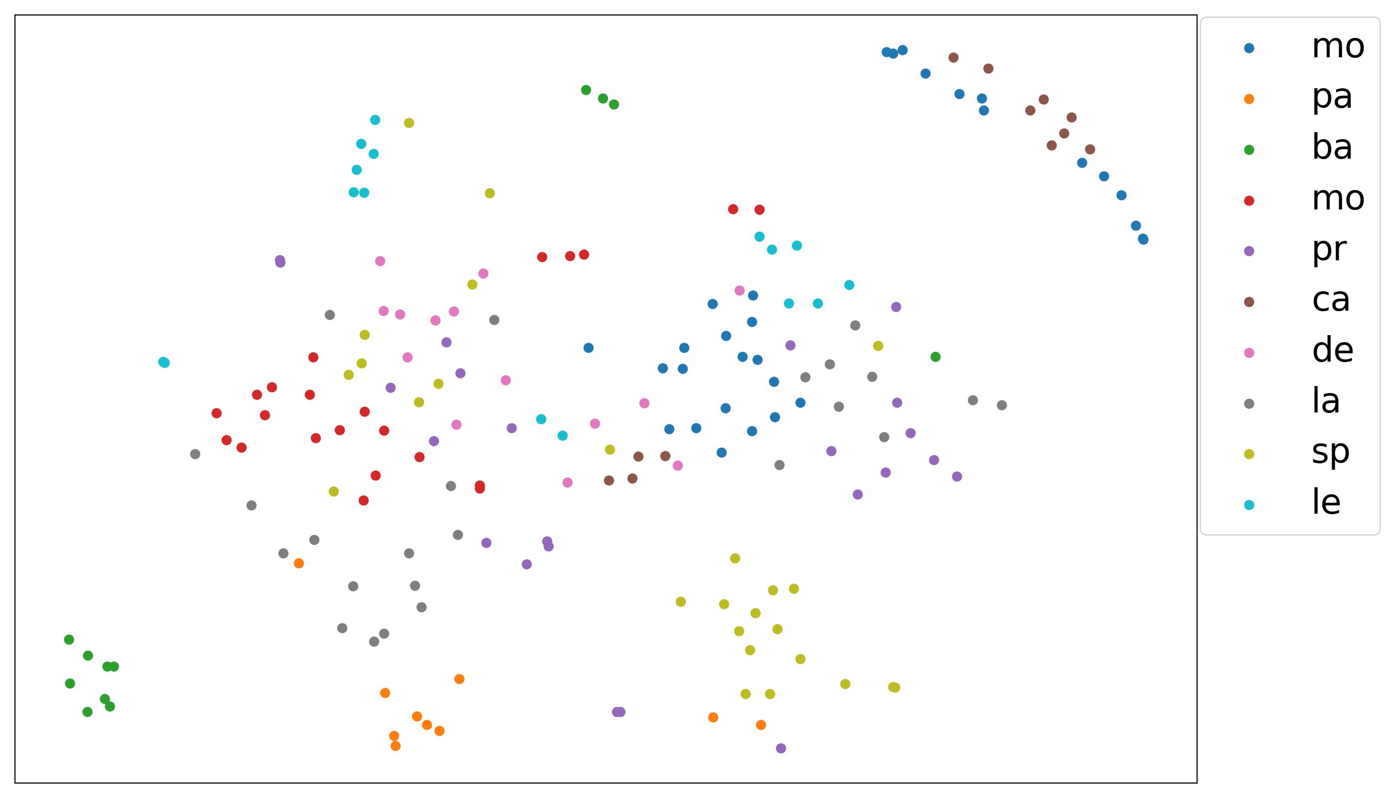
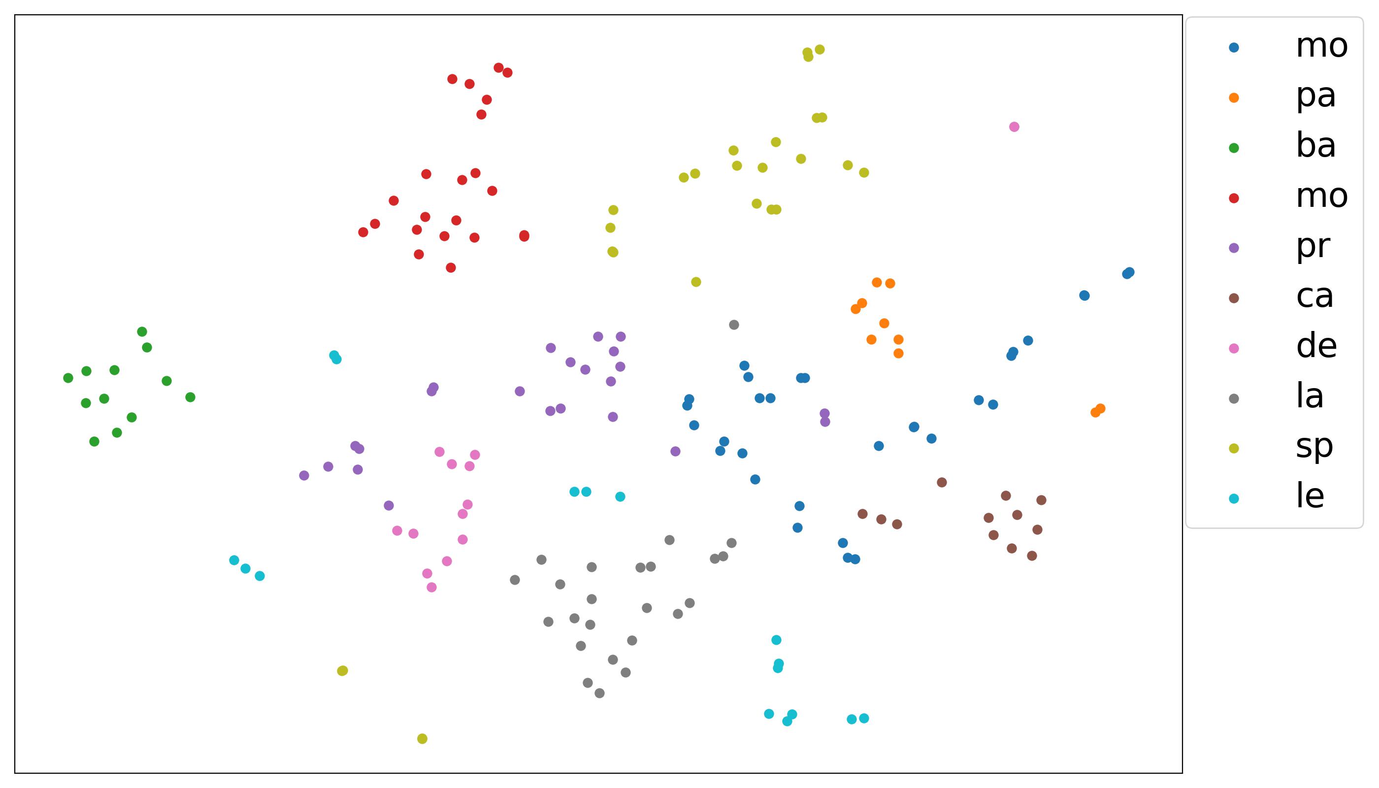
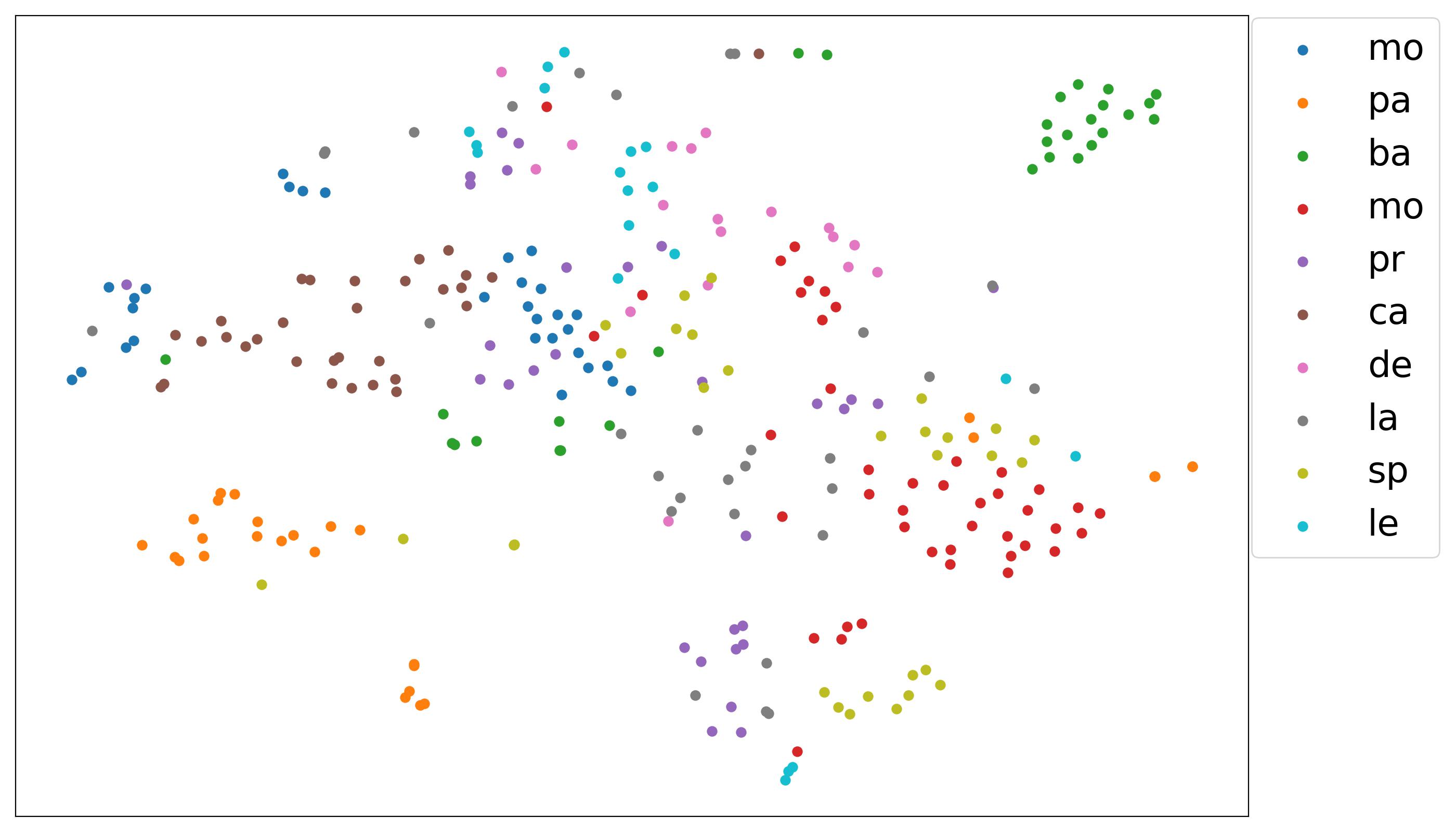
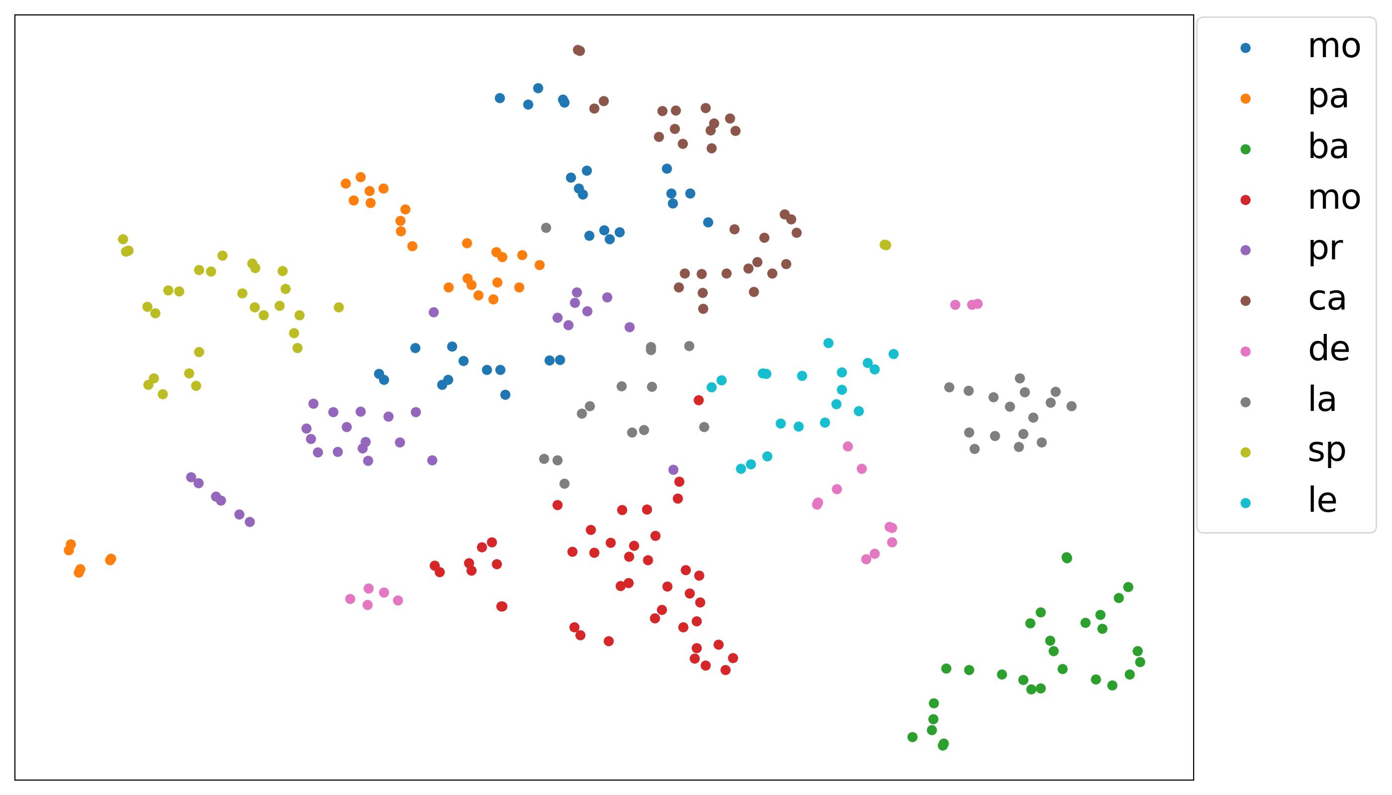
In Table 1 and 3, we present the accuracy results for the primal-PGW, UGW, and the proposed PGW methods when using three different initialization methods: POT, FLB-UOT, and FLB-POT.

Following [10], in the primal-PGW and PGW methods, we incorporate the prior knowledge $\pi$ into the definition of $p$ and $q$. Thus it is sufficient to set $mass=\pi$ for primal-PGW and choose a sufficiently large value for $\lambda$ in the PGW method. This configuration ensures that the mass matched in the target domain $\mathcal{Y}$ is exactly equal to $\pi$. However, in the UGW method [44], the setting is $p=\frac{1}{n}1_{n}$ and $q=\frac{1}{m}1_{m}$. Therefore, in each experiment, we test different parameters $(\rho,\rho_{2},\epsilon)$ and select the ones that result in transported mass close to $\pi$.

Overall, all methods show improved performance in MNIST and EMNIST datasets. One possible reason for this could be the better separability of the embeddings in MNIST and EMNIST, as illustrated in Figure 3. Additionally, since primal-PGW and PGW incorporate information from $r$ into their formulations, in many experiments, they exhibit slightly better accuracy.

(a) MNIST

(b) EMNIST

(c) Surf(A)

(d) Decaf(A)

(e) Surf(D)

(f) Decaf(D)

(g) Surf(W)

(h) Decaf(w)

Figure 3: TSNE visulization for datasets MNIST,EMNIST,Caltech Office.

References

- [1] David Alvarez-Melis and Tommi Jaakkola. Gromov-wasserstein alignment of word embedding spaces. In Proceedings of the 2018 Conference on Empirical Methods in Natural Language Processing, pages 1881–1890, 2018.
- [2] Martin Arjovsky, Soumith Chintala, and Léon Bottou. Wasserstein generative adversarial networks. In International conference on machine learning, pages 214–223. PMLR, 2017.
- [3] Yikun Bai, Bernhard Schmitzer, Matthew Thorpe, and Soheil Kolouri. Sliced optimal partial transport. In Proceedings of the IEEE/CVF Conference on Computer Vision and Pattern Recognition, pages 13681–13690, 2023.
- [4] Jessa Bekker and Jesse Davis. Learning from positive and unlabeled data: A survey. Machine Learning, 109:719–760, 2020.
- [5] Jean-David Benamou, Guillaume Carlier, Marco Cuturi, Luca Nenna, and Gabriel Peyré. Iterative bregman projections for regularized transportation problems. SIAM Journal on Scientific Computing, 37(2):A1111–A1138, 2015.
- [6] Jean-David Benamou, Brittany D Froese, and Adam M Oberman. Numerical solution of the optimal transportation problem using the monge–ampère equation. Journal of Computational Physics, 260:107–126, 2014.
- [7] Nicolas Bonneel and David Coeurjolly. SPOT: sliced partial optimal transport. ACM Transactions on Graphics, 38(4):1–13, 2019.
- [8] Alexander M Bronstein, Michael M Bronstein, and Ron Kimmel. Generalized multidimensional scaling: a framework for isometry-invariant partial surface matching. Proceedings of the National Academy of Sciences, 103(5):1168–1172, 2006.
- [9] Luis A Caffarelli and Robert J McCann. Free boundaries in optimal transport and monge-ampere obstacle problems. Annals of mathematics, pages 673–730, 2010.
- [10] Laetitia Chapel, Mokhtar Z Alaya, and Gilles Gasso. Partial optimal tranport with applications on positive-unlabeled learning. Advances in Neural Information Processing Systems, 33:2903–2913, 2020.
- [11] Lenaic Chizat, Gabriel Peyré, Bernhard Schmitzer, and François-Xavier Vialard. An interpolating distance between optimal transport and Fisher–Rao metrics. Foundations of Computational Mathematics, 18(1):1–44, 2018.
- [12] Lenaic Chizat, Gabriel Peyré, Bernhard Schmitzer, and François-Xavier Vialard. Scaling algorithms for unbalanced optimal transport problems. Mathematics of Computation, 87(314):2563–2609, 2018.
- [13] Lenaic Chizat, Gabriel Peyré, Bernhard Schmitzer, and François-Xavier Vialard. Unbalanced optimal transport: Dynamic and Kantorovich formulations. Journal of Functional Analysis, 274(11):3090–3123, 2018.
- [14] Nicolas Courty, Rémi Flamary, Amaury Habrard, and Alain Rakotomamonjy. Joint distribution optimal transportation for domain adaptation. Advances in neural information processing systems, 30, 2017.
- [15] Marco Cuturi. Sinkhorn distances: Lightspeed computation of optimal transport. Advances in neural information processing systems, 26, 2013.
- [16] Nicolò De Ponti and Andrea Mondino. Entropy-transport distances between unbalanced metric measure spaces. Probability Theory and Related Fields, 184(1-2):159–208, 2022.
- [17] Jeff Donahue, Yangqing Jia, Oriol Vinyals, Judy Hoffman, Ning Zhang, Eric Tzeng, and Trevor Darrell. Decaf: A deep convolutional activation feature for generic visual recognition. In International conference on machine learning, pages 647–655. PMLR, 2014.
- [18] Charles Elkan and Keith Noto. Learning classifiers from only positive and unlabeled data. In Proceedings of the 14th ACM SIGKDD international conference on Knowledge discovery and data mining, pages 213–220, 2008.
- [19] Kilian Fatras, Thibault Séjourné, Rémi Flamary, and Nicolas Courty. Unbalanced minibatch optimal transport; applications to domain adaptation. In International Conference on Machine Learning, pages 3186–3197. PMLR, 2021.
- [20] Alessio Figalli. The optimal partial transport problem. Archive for rational mechanics and analysis, 195(2):533–560, 2010.
- [21] Alessio Figalli and Nicola Gigli. A new transportation distance between non-negative measures, with applications to gradients flows with dirichlet boundary conditions. Journal de mathématiques pures et appliquées, 94(2):107–130, 2010.
- [22] Rémi Flamary, Nicolas Courty, Alexandre Gramfort, Mokhtar Z. Alaya, Aurélie Boisbunon, Stanislas Chambon, Laetitia Chapel, Adrien Corenflos, Kilian Fatras, Nemo Fournier, Léo Gautheron, Nathalie T.H. Gayraud, Hicham Janati, Alain Rakotomamonjy, Ievgen Redko, Antoine Rolet, Antony Schutz, Vivien Seguy, Danica J. Sutherland, Romain Tavenard, Alexander Tong, and Titouan Vayer. Pot: Python optimal transport. Journal of Machine Learning Research, 22(78):1–8, 2021.
- [23] Marguerite Frank, Philip Wolfe, et al. An algorithm for quadratic programming. Naval research logistics quarterly, 3(1-2):95–110, 1956.
- [24] Justin Gilmer, Samuel S Schoenholz, Patrick F Riley, Oriol Vinyals, and George E Dahl. Neural message passing for quantum chemistry. In International conference on machine learning, pages 1263–1272. PMLR, 2017.
- [25] Kevin Guittet. Extended Kantorovich norms: a tool for optimization. PhD thesis, INRIA, 2002.
- [26] Ishaan Gulrajani, Faruk Ahmed, Martin Arjovsky, Vincent Dumoulin, and Aaron C Courville. Improved training of wasserstein gans. Advances in neural information processing systems, 30, 2017.
- [27] Florian Heinemann, Marcel Klatt, and Axel Munk. Kantorovich–rubinstein distance and barycenter for finitely supported measures: Foundations and algorithms. Applied Mathematics & Optimization, 87(1):4, 2023.
- [28] Yu-Guan Hsieh, Gang Niu, and Masashi Sugiyama. Classification from positive, unlabeled and biased negative data. In International Conference on Machine Learning, pages 2820–2829. PMLR, 2019.
- [29] Masahiro Kato, Takeshi Teshima, and Junya Honda. Learning from positive and unlabeled data with a selection bias. In International conference on learning representations, 2018.
- [30] Soheil Kolouri, Navid Naderializadeh, Gustavo K Rohde, and Heiko Hoffmann. Wasserstein embedding for graph learning. In International Conference on Learning Representations, 2020.
- [31] Simon Lacoste-Julien. Convergence rate of frank-wolfe for non-convex objectives. arXiv preprint arXiv:1607.00345, 2016.
- [32] Jan Lellmann, Dirk A Lorenz, Carola Schonlieb, and Tuomo Valkonen. Imaging with kantorovich–rubinstein discrepancy. SIAM Journal on Imaging Sciences, 7(4):2833–2859, 2014.
- [33] Matthias Liero, Alexander Mielke, and Giuseppe Savare. Optimal entropy-transport problems and a new Hellinger–Kantorovich distance between positive measures. Inventiones mathematicae, 211(3):969–1117, 2018.
- [34] Weijie Liu, Chao Zhang, Jiahao Xie, Zebang Shen, Hui Qian, and Nenggan Zheng. Partial gromov-wasserstein learning for partial graph matching. arXiv preprint arXiv:2012.01252, 2020.
- [35] Xinran Liu, Yikun Bai, Huy Tran, Zhanqi Zhu, Matthew Thorpe, and Soheil Kolouri. Ptlp: Partial transport distances. In NeurIPS 2023 Workshop Optimal Transport and Machine Learning, 2023.
- [36] Facundo Mémoli. Spectral gromov-wasserstein distances for shape matching. In 2009 IEEE 12th International Conference on Computer Vision Workshops, ICCV Workshops, pages 256–263. IEEE, 2009.
- [37] Facundo Mémoli. Gromov–wasserstein distances and the metric approach to object matching. Foundations of computational mathematics, 11:417–487, 2011.
- [38] Nicolas Papadakis, Gabriel Peyré, and Edouard Oudet. Optimal transport with proximal splitting. SIAM Journal on Imaging Sciences, 7(1):212–238, 2014.
- [39] Gabriel Peyré, Marco Cuturi, et al. Computational optimal transport: With applications to data science. Foundations and Trends® in Machine Learning, 11(5-6):355–607, 2019.
- [40] Gabriel Peyré, Marco Cuturi, and Justin Solomon. Gromov-wasserstein averaging of kernel and distance matrices. In International conference on machine learning, pages 2664–2672. PMLR, 2016.
- [41] Benedetto Piccoli and Francesco Rossi. Generalized wasserstein distance and its application to transport equations with source. Archive for Rational Mechanics and Analysis, 211(1):335–358, 2014.
- [42] Kate Saenko, Brian Kulis, Mario Fritz, and Trevor Darrell. Adapting visual category models to new domains. In Computer Vision–ECCV 2010: 11th European Conference on Computer Vision, Heraklion, Crete, Greece, September 5-11, 2010, Proceedings, Part IV 11, pages 213–226. Springer, 2010.
- [43] Filippo Santambrogio. Optimal transport for applied mathematicians. Birkäuser, NY, 55(58-63):94, 2015.
- [44] Thibault Séjourné, François-Xavier Vialard, and Gabriel Peyré. The unbalanced gromov wasserstein distance: Conic formulation and relaxation. Advances in Neural Information Processing Systems, 34:8766–8779, 2021.
- [45] Karl-Theodor Sturm. The space of spaces: curvature bounds and gradient flows on the space of metric measure spaces, volume 290. American Mathematical Society, 2023.
- [46] Alexis Thual, Quang Huy TRAN, Tatiana Zemskova, Nicolas Courty, Rémi Flamary, Stanislas Dehaene, and Bertrand Thirion. Aligning individual brains with fused unbalanced gromov wasserstein. Advances in Neural Information Processing Systems, 35:21792–21804, 2022.
- [47] Vayer Titouan, Nicolas Courty, Romain Tavenard, and Rémi Flamary. Optimal transport for structured data with application on graphs. In International Conference on Machine Learning, pages 6275–6284. PMLR, 2019.
- [48] Cedric Villani. Optimal transport: old and new. Springer, 2009.
- [49] Cédric Villani. Topics in optimal transportation, volume 58. American Mathematical Soc., 2021.
- [50] Hongteng Xu, Dixin Luo, and Lawrence Carin. Scalable gromov-wasserstein learning for graph partitioning and matching. Advances in neural information processing systems, 32, 2019.
- [51] Hongteng Xu, Dixin Luo, Hongyuan Zha, and Lawrence Carin Duke. Gromov-wasserstein learning for graph matching and node embedding. In International conference on machine learning, pages 6932–6941. PMLR, 2019.