Cross-Task Linearity Emerges in the Pretraining-Finetuning Paradigm

Abstract

The pretraining-finetuning paradigm has become the prevailing trend in modern deep learning. In this work, we discover an intriguing linear phenomenon in models that are initialized from a common pretrained checkpoint and finetuned on different tasks, termed as Cross-Task Linearity (CTL). Specifically, if we linearly interpolate the weights of two finetuned models, the features in the weight-interpolated model are approximately equal to the linear interpolation of features in two finetuned models at each layer. Such cross-task linearity has not been noted in peer literature. We provide comprehensive empirical evidence supporting that CTL consistently occurs for finetuned models that start from the same pretrained checkpoint. We conjecture that in the pretraining-finetuning paradigm, neural networks essentially function as linear maps, mapping from the parameter space to the feature space. Based on this viewpoint, our study unveils novel insights into explaining model merging/editing, particularly by translating operations from the parameter space to the feature space. Furthermore, we delve deeper into the underlying factors for the emergence of CTL, emphasizing the impact of pretraining.

1 Introduction

Pretrained models have become the fundamental infrastructure of modern machine learning systems, and finetuning has evolved as a predominant way for adapting the pretrained model to various downstream tasks. Despite the prominent success, our understanding of the pretraining-finetuning paradigm still lags behind. There is a growing interest in unraveling the hidden mechanisms of pretraining and finetuning, particularly in human preference alignment [45], interpretability [8, 43], and AI ethics [55].

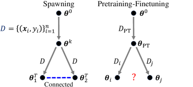
Figure 1: The spawning method and the pretraining-finetuning paradigm. $\boldsymbol{\theta}^{0}$ denotes random initialization of the network weights. For spawning, the network is first trained for $k$ epochs, i.e., $\boldsymbol{\theta}^{k}$, then spawned into two copies and updated until convergence, i.e, $\boldsymbol{\theta}_{1}^{T},\boldsymbol{\theta}_{2}^{T}$. Note that $\boldsymbol{\theta}_{1}^{T},\boldsymbol{\theta}_{2}^{T}$ are trained on the same dataset as $\boldsymbol{\theta}^{k}$ but with different SGD randomness. With a proper chosen $k$ ($k$ is small in practical scenarios, e.g., $5$ epochs for ResNet-20 on CIFAR-10), $\boldsymbol{\theta}_{1}^{T}$ and $\boldsymbol{\theta}_{2}^{T}$ can satisfy LMC and LLFC simultaneously. For pretraining-finetuning, the network is first trained on pretraining dataset $\mathcal{D}_{\rm PT}$ to get $\boldsymbol{\theta}_{\rm PT}$. Then $\boldsymbol{\theta}_{\rm PT}$ is finetuned on $\mathcal{D}_{i}$ and $\mathcal{D}_{j}$ to get $\boldsymbol{\theta}_{i}$ and $\boldsymbol{\theta}_{j}$, where $\mathcal{D}_{i}$ and $\mathcal{D}_{j}$ are different datasets.

Recent works on Linear Mode Connectivity (LMC) [38, 13] and Layerwise Linear Feature Connectivity (LLFC) [63] shed light on understanding the training dynamics and hidden mechanisms of neural networks. LMC depicts a linear path in the parameter space of a network where the loss remains approximately constant (see Definition 1). In other words, linearly interpolating the weights of two different models, which are of the same architecture and trained on the same task, could lead to a new model that achieves similar performance as the two original models. LLFC indicates that the features in the weight-interpolated model are proportional to the linear interpolation of the features in the two original models (see Definition 2). Frankle et al. [13] observed LMC for networks that are jointly trained for a short time before undergoing independent training on the same dataset, termed as spawning method (see Figure 1). Zhou et al. [63] discovered the models that linearly connected in the loss landscape are also linearly connected in feature space, i.e., satisfy LMC and LLFC simultaneously.

	Performance	Equality	Task
LMC [13]	Approx. equal	Approx. equal	Single
LLFC [63]	Flexible	Proportional to	Single
CTL (Ours)	Flexible	Approx. equal	Multiple

Table 1: Comparison: LMC requires models with approximately equal performance. LLFC depicts a proportional relationship only. Previous studies on LMC and LLFC focus on models trained on the same task. Our work extends LLFC to models finetuned on different tasks, which further induces CTL.

As shown in Figure 1, a connection is identified between the pretraining-finetuning paradigm and the spawning method, as both entail training models from a same pretrained checkpoint. Therefore, a natural question arises: are models, initialized from a common pretrained checkpoint but finetuned on different tasks, linearly connected in the loss landscape or feature space, akin to the models obtained by the spawning method satisfying LMC and LLFC?

In this work, we discover that the finetuned models are linearly connected in internal features even though there is no such connectivity in the loss landscape, i.e., LLFC holds but LMC not. Indeed, we identify a stronger notion of linearity than LLFC: if we linearly interpolate the weights of two models that finetuned on different tasks, the features in the weight-interpolated model are approximately equal to the linear interpolation of features in the two finetuned models at each layer, namely Cross-Task Linearity (CTL) (see comparison among LMC, LLFC, and CTL in Table 1). To be precise, let $\boldsymbol{\theta}_{i}$ and $\boldsymbol{\theta}_{j}$ be the weights of two finetuned models, and $f^{(\ell)}(\boldsymbol{\theta})$ be the features in the model of weights $\boldsymbol{\theta}$ at $\ell$-th layer. We say that $\boldsymbol{\theta}_{i}$ and $\boldsymbol{\theta}_{j}$ satisfy CTL if $\forall\ell,\forall\alpha\in[0,1]$,

$$f^{(\ell)}(\alpha{\boldsymbol{\theta}}_{i}+(1-\alpha){\boldsymbol{\theta}}_{j})\approx\alpha f^{(\ell)}({\boldsymbol{\theta}}_{i})+(1-\alpha)f^{(\ell)}({\boldsymbol{\theta}}_{j}).$$

Certainly, CTL may not be universal for arbitrary networks trained on different tasks, yet we provide comprehensive empirical evidence supporting that CTL consistently occurs for the finetuned models that start from a common pretrained checkpoint across a wide range of settings. Hence, we conjecture that in the pretraining-finetuning paradigm, neural networks essentially function as linear maps, mapping from the parameter space to the feature space.

From the observed CTL in the pretraining-finetuning paradigm, we obtain novel insights into two widely-used model merging/editing techniques: model averaging [21, 35, 50, 49, 56, 57] and task arithmetic [19, 20, 44].

i) Model averaging takes the average of weights of multiple models, which are finetuned on the same dataset but with different hyperparameter configurations, so as to improve accuracy and robustness. We explain the averaging of weights as the averaging of features at each layer, building a stronger connection between model averaging and logits ensemble than before.

ii) Task arithmetic merges the weights of models, that are finetuned on different tasks, via simple arithmetic operations, shaping the behaviour of the resulting model accordingly. We translate the arithmetic operation in the parameter space into the operations in the feature space, yielding a feature-learning explanation for task arithmetic.

Furthermore, we delve deeper into the root cause of CTL and underscore the impact of pretraining. We empirically show that the common knowledge acquired from the pretraining stage contributes to the satisfaction of CTL. We also take a primary attempt to prove CTL and find that the emergence of CTL is associated with the flatness of the network landscape and the distance between the weights of two finetuned models.

In summary, our work reveals a linear connection between finetuned models, offering significant insights into model merging/editing techniques. This, in turn, advances our understanding of underlying mechanisms of pretraining and finetuning from a feature-centric perspective.

2 Related Work

(Linear) Mode Connectivity. Freeman and Bruna [15], Draxler et al. [7], Garipov et al. [16] noted Mode Connectivity (MC), where different minima in the loss landscape can be connected by a non-linear path of nearly constant loss. Nagarajan and Kolter [38], Frankle et al. [13] discovered that the path of nearly constant loss can be linear, for models that are jointly trained for a short time before undergoing independent training, termed Linear Mode Connectivity (LMC). Fort et al. [12] analyzed LMC from a perspective of the Neural Tangent Kernel dynamics. Entezari et al. [9], Ainsworth et al. [2] showed that even independently trained networks can satisfy LMC after accounting for permutation invariance. Studies [31, 54, 41, 40, 26, 11, 62] have attempted to prove (linear) mode connectivity from various perspectives. Adilova et al. [1] studied the layerwise behaviour of LMC under federated learning settings. Yunis et al. [61] extended LMC to the case of multiple modes and identified a high-dimensional convex hull of low loss in the loss landscape. Qin et al. [46] studied MC in the context of pretrained language models. Mirzadeh et al. [37], Juneja et al. [23] investigated finetuning from the lens of LMC. Zhou et al. [63] identified a stronger connectivity than LMC, namely Layerwise Linear Feature Connectivity (LLFC), and observed LLFC always co-occurs with LMC.

Model Merging/Editing. Recent studies find averaging the parameters of finetuned models over same datasets leads to improved performance and generalization abilities [21, 35, 50, 49, 56, 57]. Moreover, the averaging of weights from models finetuned over tasks enables multi-task abilities [19, 30, 59, 22, 53, 60]. Singh and Jaggi [51], Liu et al. [33] show that the weights of independently trained neural networks can be merged after aligning the neurons. Moreover, Ilharco et al. [20], Ortiz-Jimenez et al. [44] extend the simple averaging to arithmetic operations in the parameter space, enabling a finer-grained control of the model behaviours.

3 Backgrounds and Preliminaries

Notation Setup. Unless explicitly stated otherwise, we consider a classification dataset, denoted as $\mathcal{D}=\{(\boldsymbol{x}_{i},y_{i})\}_{i=1}^{n}$ where $\boldsymbol{x}_{i}\in\mathbb{R}^{d_{0}}$ is the input and $y_{i}\in[c]$ is the label of the $i$-th datapoint. Here, $d_{0}$ is the input dimension, $[c]=\{1,2,\ldots,c\}$ and $c$ is the number of classes. We use ${\boldsymbol{X}}\in\mathbb{R}^{d_{0}\times n}$ to stack all the input data into a matrix.

We consider an $L$-layer neural network defined as $f(\boldsymbol{\theta};\boldsymbol{x})$, where $\boldsymbol{\theta}$ denotes the model parameters, $\boldsymbol{x}$ is the input, and $f(\boldsymbol{\theta};\boldsymbol{x})\in\mathbb{R}^{c}$. $f^{(\ell)}(\boldsymbol{\theta};\boldsymbol{x})\in\mathbb{R}^{d_{\ell}}$ represents the internal feature (post-activation) in the network at the $\ell$-th layer. Here, $d_{\ell}$ denotes the dimension of the $\ell$-th layer ($0\leq\ell\leq L$) and $f^{(L)}(\boldsymbol{\theta};\boldsymbol{x})=f(\boldsymbol{\theta};\boldsymbol{x})$. For an input matrix $\boldsymbol{X}$, we use $f^{(\ell)}(\boldsymbol{\theta};\boldsymbol{X})\in\mathbb{R}^{d_{\ell}\times n}$ to denote the collection of features on all the datapoints. When $\boldsymbol{X}$ is clear from the context, we simply write $f^{(\ell)}(\boldsymbol{\theta})=f^{(\ell)}(\boldsymbol{\theta};\boldsymbol{X})$. The expected loss on dataset $\mathcal{D}$ is denoted by $\mathcal{L}(\boldsymbol{\theta})=\mathbb{E}_{(\boldsymbol{x},y)\in\mathcal{D}}\left[L\left(f\left(\boldsymbol{\theta};\boldsymbol{x}\right),y\right)\right]$, where $L$ represents the loss function. Our analysis focuses on models trained on a training set, with all investigations evaluated on a separate test set.

Experimental Setup. Due to space limit, we defer detailed experimental settings to Section B.1.

Linear Mode Connectivity (LMC).

Definition 1 (Linear Mode Connectivity [38, 13]).

Given dataset $\mathcal{D}$ and two modes ${\boldsymbol{\theta}}_{i}$ and ${\boldsymbol{\theta}}_{j}$ such that $\mathcal{L}({\boldsymbol{\theta}}_{i})\approx\mathcal{L}({\boldsymbol{\theta}}_{j})$ on $\mathcal{D}$, we say ${\boldsymbol{\theta}}_{i}$ and ${\boldsymbol{\theta}}_{j}$ are linearly connected in the loss landscape if they satisfy $\forall\alpha\in[0,1]$,

$$\mathcal{L}(\alpha{\boldsymbol{\theta}}_{i}+(1-\alpha){\boldsymbol{\theta}}_{j})\approx\mathcal{L}({\boldsymbol{\theta}}_{i})\approx\mathcal{L}({\boldsymbol{\theta}}_{j}).$$

As Definition 1 shows, LMC indicates different optima can be connected via a simple linear path of nearly constant loss. Previous studies [13, 12] observed LMC for networks that start from a common pretrained checkpoint and undergo independent training on the same task until convergence, commonly referred as spawning method.

Layerwise Linear Feature Connectivity (LLFC).

Definition 2 (Layerwise Linear Feature Connectivity [63]).

Given dataset $\mathcal{D}$ and two modes ${\boldsymbol{\theta}}_{i}$, ${\boldsymbol{\theta}}_{j}$ of an $L$-layer neural network $f$, the modes ${\boldsymbol{\theta}}_{i}$ and ${\boldsymbol{\theta}}_{j}$ are said to be linearly connected in feature space on $\mathcal{D}$ if $\forall\ell\in[L],\forall\alpha\in[0,1]$ such that,

$$f^{(\ell)}(\alpha{\boldsymbol{\theta}}_{i}+(1-\alpha){\boldsymbol{\theta}}_{j})\propto\alpha f^{(\ell)}({\boldsymbol{\theta}}_{i})+(1-\alpha)f^{(\ell)}({\boldsymbol{\theta}}_{j}).$$

In Definition 2, LLFC states that the features (post-activation) in the interpolated model $\boldsymbol{\theta}_{\alpha}=\alpha\boldsymbol{\theta}_{i}+(1-\alpha)\boldsymbol{\theta}_{j}$ are proportional to the linear interpolation of the features in $\boldsymbol{\theta}_{i}$ and $\boldsymbol{\theta}_{j}$ at each layer.

Zhou et al. [63] introduced LLFC, which defines a stronger notion of linear connectivity than LMC, and noted its consistent co-occurrence with LMC. Specifically, if two modes $\boldsymbol{\theta}_{i}$ and $\boldsymbol{\theta}_{j}$ satisfy LMC, then they also approximately satisfy LLFC. Moreover, it can be proven that LLFC directly induces LMC for models with equal loss (see Lemma 1). Therefore, they believed that LLFC is a more fundamental property than LMC.

Lemma 1 (LLFC Induces LMC (Proof in Section A.1)).

Given dataset $\mathcal{D}$, convex loss function $L$, and two modes ${\boldsymbol{\theta}}_{i}$ and ${\boldsymbol{\theta}}_{j}$ with equal loss on $\mathcal{D}$, i.e., $\mathcal{L}({\boldsymbol{\theta}}_{i})=\mathcal{L}({\boldsymbol{\theta}}_{j})$, suppose the two modes ${\boldsymbol{\theta}}_{i}$, ${\boldsymbol{\theta}}_{j}$ satisfy LLFC on $\mathcal{D}$ with exact equality, then for all $\alpha\in[0,1]$,

$$\mathcal{L}(\alpha{\boldsymbol{\theta}}_{i}+(1-\alpha){\boldsymbol{\theta}}_{j})\leq\mathcal{L}(\boldsymbol{\theta}_{i})=\mathcal{L}(\boldsymbol{\theta}_{j}).$$

4 Cross-Task Linearity

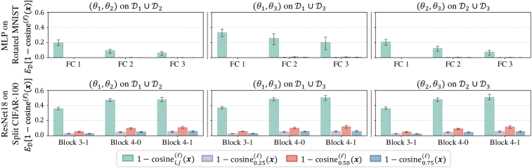
Figure 2: Compare $\mathbb{E}_{\mathcal{D}}[1-{\rm cosine}_{\alpha}^{(\ell)}(\boldsymbol{x})]$ with $\mathbb{E}_{\mathcal{D}}[1-\text{cosine}_{i,j}^{(\ell)}(\boldsymbol{x})]$. Here, $\{\boldsymbol{\theta}_{i}\}_{i=1}^{3}$ and $\{\mathcal{D}_{i}\}_{i=1}^{3}$ denotes three finetuned models and their corresponding downstream tasks. For Rotated MNIST, models are pretrained on MNIST and finetuned on variants of MNIST where digits are at different angles. For Split CIFAR-100, models are pretrained and finetuned on disjoint sets of 5 classes from CIFAR-100. The bottom and top of the error bar represent the lower and upper quartile of the values across the dataset, respectively. The results are reported for last three layers/blocks of finetuned models, with $\alpha\in\{0.25,0.5,0.75\}$. More results in Section B.4.

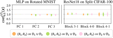
Figure 3: Distribution of $\text{coef}_{\alpha}^{(\ell)}(\boldsymbol{x})$ across the dataset. Here, $\alpha=0.5$. $\{\boldsymbol{\theta}_{i}\}_{i=1}^{3}$ and $\{\mathcal{D}_{i}\}_{i=1}^{3}$ denotes three finetuned models and their corresponding downstream tasks, following the same training settings as in Figure 2. The results are reported for last three layers/blocks of finetuned models. More results in Section B.4 (include results for $\alpha\in\{0.25,0.75\}$).

In this section, we provide empirical evidence indicating that the finetuned models are linearly connected in the feature space, even though there is no such connectivity in the loss landscape, i.e. LLFC holds but LMC not. Taking a step further, we identify a stronger notion of linearity, namely Cross-Task Linearity (CTL), which approximately characterizing neural networks as linear maps in the pretraining-finetuning paradigm. From these observations, we offer novel insights into model averaging and task arithmetic.

4.1 Extend LMC and LLFC to CTL

LMC Fails in the Pretraining-Finetuning Paradigm. LMC might not hold for the finetuned models, as the pre-conditions of Definition 1 are not met, i.e., the models finetuned on different tasks might not have approximately equal optimal loss on the same dataset. Indeed, the studies on LMC are motivated by the interest in studying optima of the same loss landscape. It means LMC depicts the property of models trained on the same dataset. Therefore, it is clear that finetuned models might not satisfy LMC, even on the pretraining task, where catastrophic forgetting may occur [36]. Similar phenomena were observed in [37, 23].

LLFC Holds in the Pretraining-Finetuning Paradigms. Despite there being no connectivity in the loss landscape, we surprisingly find that the finetuned models are linearly connected in the feature space. Here, we extend the original LLFC to the cases where models are finetuned on different datasets.

To verify LLFC for finetuned models, we conduct extensive experiments across a range of settings. Specifically, we consider a set of finetuned models, $\boldsymbol{\Theta}=\{\boldsymbol{\theta}_{i}\}_{i=1}^{k}$, which are initialized from a common pretrained checkpoint $\boldsymbol{\theta}_{\rm PT}$ but finetuned on different tasks. Here, the downstream tasks for finetuning are denoted as $\{\mathcal{D}_{i}\}_{i=1}^{k}$, respectively. Then, for each pair of finetuned models $(\boldsymbol{\theta}_{i},\boldsymbol{\theta}_{j})\in\boldsymbol{\Theta}^{2}$, on each datapoint $(\boldsymbol{x},\boldsymbol{y})\in\mathcal{D}_{i}\cup\mathcal{D}_{j}$, we measure the cosine similarity between the features in the weight-interpolated model $\boldsymbol{\theta}_{\alpha}=\alpha\boldsymbol{\theta}_{i}+(1-\alpha)\boldsymbol{\theta}_{j}$ and the linear interpolation of the features in $\boldsymbol{\theta}_{i}$ and $\boldsymbol{\theta}_{j}$ at each layer $\ell$, denoted as $\text{cosine}_{\alpha}^{(\ell)}(\boldsymbol{x})=\cos[f^{(\ell)}(\boldsymbol{\theta}_{\alpha};\boldsymbol{x}),\alpha f^{(\ell)}(\boldsymbol{\theta}_{i};\boldsymbol{x})+(1-\alpha)f^{(\ell)}(\boldsymbol{\theta}_{j};\boldsymbol{x})]$. We compare $\text{cosine}_{\alpha}^{(\ell)}$ to the baseline cosine similarity between the features in $\boldsymbol{\theta}_{i}$ and $\boldsymbol{\theta}_{j}$ in the same layer, i.e, $\text{cosine}_{i,j}^{(\ell)}(\boldsymbol{x})=\cos[f^{(\ell)}(\boldsymbol{\theta}_{i};\boldsymbol{x}),f^{(\ell)}(\boldsymbol{\theta}_{j};\boldsymbol{x})]$. In Figure 2, the values of $\mathbb{E}_{\mathcal{D}}[1-{\rm cosine}_{\alpha}^{(\ell)}(\boldsymbol{x})]$ consistently approach $0$ across a range of layers, $\alpha$, and various pairs of $(\boldsymbol{\theta}_{i},\boldsymbol{\theta}_{j})$, under different task settings. The small error bars indicate a consistent behaviour across each datapoint in $\mathcal{D}_{i}\cup\mathcal{D}_{j}$. Additionally, the values of baseline $\mathbb{E}_{\mathcal{D}}[1-\text{cosine}_{i,j}^{(\ell)}(\boldsymbol{x})]$ deviate from $0$, excluding the trivial scenario where $f^{(\ell)}({\boldsymbol{\theta}}_{i})$ and $f^{(\ell)}({\boldsymbol{\theta}}_{j})$ are already close enough. The results confirm that LLFC holds in the pretraining-finetuning paradigm.

CTL Occurs in the Pretraining-Finetuning Paradigm. Building upon the observations of LLFC for finetuned models, we identify a stronger notion of linearity than LLFC, termed as Cross-Task Linearity (CTL). Precisely, given a pair of finetuned models $(\boldsymbol{\theta}_{i},\boldsymbol{\theta}_{j})\in\boldsymbol{\Theta}^{2}$ and downstream tasks $\mathcal{D}_{i}$ and $\mathcal{D}_{j}$ respectively, we say them satisfy CTL on $\mathcal{D}_{i}\cup\mathcal{D}_{j}$ if $\forall\ell\in[L],\forall\alpha\in[0,1]$,

$$f^{(\ell)}(\alpha{\boldsymbol{\theta}}_{i}+(1-\alpha){\boldsymbol{\theta}}_{j})\approx\alpha f^{(\ell)}({\boldsymbol{\theta}}_{i})+(1-\alpha)f^{(\ell)}({\boldsymbol{\theta}}_{j}).$$

Beyond LLFC, CTL enforces the approximate equality. We have validated the features in weight-interpolated model $\boldsymbol{\theta}_{\alpha}$ and the linear interpolation of features in $\boldsymbol{\theta}_{i}$ and $\boldsymbol{\theta}_{j}$ have similar directions. To further validate CTL, we compare the length of their features at each layer $\ell$. Specifically, for each pair of finetuned models $(\boldsymbol{\theta}_{i},\boldsymbol{\theta}_{j})\in\boldsymbol{\Theta}^{2}$, on each datapoint $\boldsymbol{x}\in\mathcal{D}_{i}\cup\mathcal{D}_{j}$, we measure ${\rm coef}_{\alpha}^{(\ell)}(\boldsymbol{x})=\frac{\|f^{(\ell)}(\boldsymbol{\theta}_{\alpha};\boldsymbol{x})\|\text{\ cosine}_{\alpha}^{(\ell)}(\boldsymbol{x})}{\|\alpha f^{(\ell)}(\boldsymbol{\theta}_{i};\boldsymbol{x})+(1-\alpha)f^{(\ell)}(\boldsymbol{\theta}_{j};\boldsymbol{x})\|}$ . In Figure 3, the values of ${\rm coef}_{\alpha}^{(\ell)}(\boldsymbol{x})$ are close to $1$ across various layers and different pairs of $(\boldsymbol{\theta}_{i},\boldsymbol{\theta}_{j})$, under different task settings.

In summary, we observe that CTL consistently occurs for the finetuned models that start from a common pretrained checkpoint. Therefore, we conjecture that neural networks approximately function as linear maps in the pretraining-finetuning paradigm, mapping from the parameter space to the feature space. This viewpoint enables us to study model merging/editing from a feature-learning perspective.

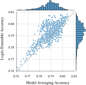
Figure 4: Linear correlation between the model averaging accuracy and the logits ensemble accuracy. Each datapoint represents three models fine-tuned on ImageNet with varying hyperparameters, denoted as $\{\boldsymbol{\theta}\}_{i=1}^{3}$. We have $20$ finetuned models and obtain $\binom{20}{3}=1140$ datapoints in total. The x-axis represents accuracy of $f(\frac{1}{3}\sum_{i=1}^{3}\boldsymbol{\theta}_{i})$, while the y-axis represents accuracy of $\frac{1}{3}\sum_{i=1}^{3}f(\boldsymbol{\theta}_{i})$. The grey dashed line represents $y=x$.

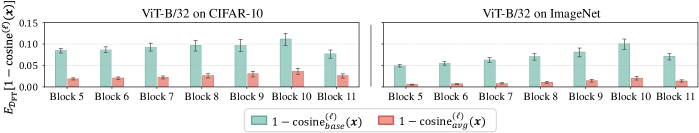
Figure 5: Compare $\mathbb{E}_{\mathcal{D}}[1-{\rm cosine}_{avg}^{(\ell)}(\boldsymbol{x})]$ with $\mathbb{E}_{\mathcal{D}}[1-{\rm cosine}_{base}^{(\ell)}(\boldsymbol{x})]$. The bottom and top of the error bar represent the lower and upper quartile of the values across the dataset, respectively. The results are reported for last $7$ blocks of ViT-B/32 models, that are finetuned on CIFAR-10 and ImageNet, respectively. More results in Section B.5.

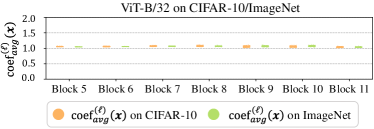
Figure 6: Distribution of ${\rm coef}_{avg}^{(\ell)}(\boldsymbol{x})$ across the dataset. The results are reported for last $7$ blocks of ViT-B/32 models, that are finetuned on CIFAR-10 and ImageNet, respectively. More results in Section B.5.

4.2 Insights into Model Averaging

Recent studies [56, 57] discovered that averaging the weights of multiple models fine-tuned on the same dataset but with different hyperparameter configurations often leads to improved accuracy and robustness. This approach, termed as model averaging, can be formulated as $f(\frac{1}{k}\sum_{i=1}^{k}\boldsymbol{\theta}_{i})$. Here, $\{\boldsymbol{\theta}_{i}\}_{i=1}^{k}$ represents the set of finetuned models, and the downstream task for finetuning is denoted as $\mathcal{D}_{\rm FT}$. Alternatively, as another way to combine multiple models, the logits ensemble simply averages the outputs of different models, i.e., $\frac{1}{k}\sum_{i=1}^{k}f(\boldsymbol{\theta}_{i})$. Both methods are effective in improving overall model performance in practice and indeed a linear correlation has been observed between the accuracy of model averaging and logits ensemble (see Figure 4). In this subsection, we build a stronger connection between model averaging and logits ensemble in the feature space.

Specifically, we discover that the features in model averaging can be approximated by the averaging of features in each individual finetuned model, i.e., $\forall\ell\in[L]$,

$$f^{(\ell)}\left(\frac{1}{k}\sum_{i=1}^{k}\boldsymbol{\theta}_{i}\right)\approx\frac{1}{k}\sum_{i=1}^{k}f^{(\ell)}({\boldsymbol{\theta}}_{i}).$$ (1)

We conduct extensive experiments to validate our discovery. Similar to Section 4.1, on each datapoint $\boldsymbol{x}\in\mathcal{D}_{\rm FT}$, we measure the cosine similarity between the features in model averaging $f^{(\ell)}(\frac{1}{k}\sum_{i=1}^{k}\boldsymbol{\theta}_{i})$ and the averaging of features in each model $\frac{1}{k}\sum_{i=1}^{k}f^{(\ell)}({\boldsymbol{\theta}}_{i})$ at each layer $\ell$, denoted as ${\rm cosine}_{avg}^{(\ell)}(\boldsymbol{x})=\cos[f^{(\ell)}(\frac{1}{k}\sum_{i=1}^{k}\boldsymbol{\theta}_{i};\boldsymbol{x}),\frac{1}{k}\sum_{i=1}^{k}f^{(\ell)}({\boldsymbol{\theta}}_{i};\boldsymbol{x})]$ Additionally, we compare ${\rm cosine}_{avg}^{(\ell)}(\boldsymbol{x})$ with the baseline ${\rm cosine}_{base}^{(\ell)}(\boldsymbol{x})=\frac{1}{k}\sum_{i=1}^{k}\cos[f^{(\ell)}(\frac{1}{k}\sum_{j=1}^{k}\boldsymbol{\theta}_{j};\boldsymbol{x}),f^{(\ell)}({\boldsymbol{\theta}}_{i};\boldsymbol{x})]$. We compute ${\rm coef}_{avg}^{(\ell)}(\boldsymbol{x})=\frac{\|f^{(\ell)}\left(\frac{1}{k}\sum_{i=1}^{k}\boldsymbol{\theta}_{i};\boldsymbol{x}\right)\|{\rm cosine}_{avg}^{(\ell)}(\boldsymbol{x})}{\|\frac{1}{k}\sum_{i=1}^{k}f^{(\ell)}({\boldsymbol{\theta}}_{i};\boldsymbol{x})\|}$ to validate the features have similar length. In Figure 5, the values of $\mathbb{E}_{\mathcal{D}}[1-{\rm cosine}_{avg}^{(\ell)}(\boldsymbol{x})]$ closely approach $0$ compared with the baseline $\mathbb{E}_{\mathcal{D}}[1-\text{cosine}_{base}^{(\ell)}(\boldsymbol{x})]$, and in Figure 6, the values of ${\rm coef}_{avg}^{(\ell)}(\boldsymbol{x})$ closely approximate $1$. In conclusion, model averaging roughly aggregates the features in each individual finetuned model at each layer.

It is not difficult to see that our discovery could directly imply the observed linear correlation between the model averaging accuracy and the logits ensemble accuracy, particularly when Equation 1 is applied to the output layer. Apparently, our discovery unveils a finer-grained characterization of the linear correlation between model averaging and logits ensemble. Indeed, our discovery can be viewed as a generalization of CTL to the case of multiple models in the pretraining-finetuning paradigm (see Lemma 2). Hence, we conclude that CTL establishes a stronger connection between model averaging and logits ensemble in the feature space, thus further explaining the effectiveness of model averaging from a feature-learning perspective.

Lemma 2 (CTL Generalizes to Multiple Models (Proof in Section A.2)).

Given dataset $\mathcal{D}$ and a field of modes $\boldsymbol{\Theta}$ where each pair of modes $(\boldsymbol{\theta}_{i},\boldsymbol{\theta}_{j})\in\boldsymbol{\Theta}^{2}$ satisfy CTL on $\mathcal{D}$, then for any $\{\boldsymbol{\theta}_{i}\}_{i=1}^{k}\in\boldsymbol{\Theta}$ and $\{\alpha_{i}\}_{i=1}^{k}\in[0,1]$, subject to the constraint that $\sum_{i=1}^{k}\alpha_{i}=1$, we have

$$f^{(\ell)}\left(\sum_{i=1}^{k}\alpha_{i}\boldsymbol{\theta}_{i}\right)\approx\sum_{i=1}^{k}\alpha_{i}f^{(\ell)}({\boldsymbol{\theta}}_{i}),\quad\forall\ell\in[L].$$

4.3 Insights into Task Arithmetic

Ilharco et al. [20] introduced task arithmetic for editing pretrained models using task vectors, which are obtained by subtracting the pretrained weights from the finetuned weights. Specifically, considering a pretrained model $\boldsymbol{\theta}_{\rm PT}$ and a set of finetuned models $\{\boldsymbol{\theta}_{i}\}_{i=1}^{k}$ for downstream tasks $\{\mathcal{D}_{i}\}_{i=1}^{k}$ respectively, the task vectors are defined as $\{\tau_{i}\}_{i=1}^{k}$, where $\tau_{i}=\boldsymbol{\theta}_{i}-\boldsymbol{\theta}_{PT}$. Arithmetic operations, including addition and negation, can be applied to the task vectors to obtain a new task vector $\tau_{\rm new}$, and the new task vector is then applied to the pretrained weights with a scaling term $\lambda$, i.e., $\boldsymbol{\theta}_{\rm new}=\boldsymbol{\theta}_{\rm PT}+\lambda\tau_{\rm new}$. It allows to control the behavior of the edited model via simple arithmetic operations on task vectors. In this subsection, we aim to explain the effectiveness of task arithmetic from a feature-learning perspective.

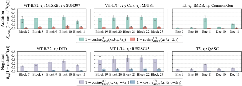
Figure 7: Addition: Compare $\mathbb{E}_{\mathcal{D}}[1-{\rm cosine}_{arith}^{(\ell)}(\boldsymbol{x};\lambda\tau_{i},\lambda\tau_{j})]$ with $\mathbb{E}_{\mathcal{D}}[1-{\rm cosine}_{base}^{(\ell)}(\boldsymbol{x};\lambda\tau_{i},\lambda\tau_{j})]$. Negation: Compare $\mathbb{E}_{\mathcal{D}}[1-{\rm cosine}_{arith}^{(\ell)}(\boldsymbol{x};\lambda\tau_{i},-\lambda\tau_{i})]$ with $\mathbb{E}_{\mathcal{D}}[1-{\rm cosine}_{base}^{(\ell)}(\boldsymbol{x};\lambda\tau_{i},-\lambda\tau_{i})]$. The bottom and top of the error bar represent the lower and upper quartile of the values across the dataset, respectively. The results are reported for last $5$ blocks of finetuned models under different settings, with $\lambda=0.4$ [20]. More results in Sections B.6 and B.7.

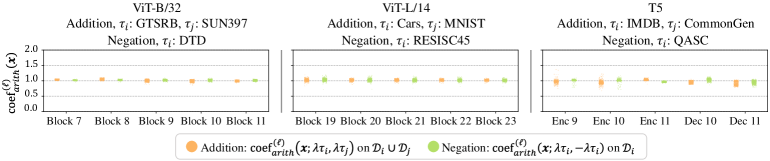
Figure 8: Addition: Distribution of ${\rm coef}_{arith}^{(\ell)}(\boldsymbol{x};\lambda\tau_{i},\lambda\tau_{j})$. Negation: Distribution of ${\rm coef}_{arith}^{(\ell)}(\boldsymbol{x};\lambda\tau_{i},-\lambda\tau_{i})$. The results are reported for last $5$ blocks of finetuned models under different settings, with $\lambda=0.4$ [20]. More results in Sections B.6 and B.7.

CTL Explains Learning via Addition. An intriguing discovery in task arithmetic is that the addition of task vectors builds multi-task models. For instance, with a proper chosen $\lambda$, $f\left(\boldsymbol{\theta}_{\rm PT}+\lambda\left(\tau_{i}+\tau_{j}\right)\right)$ demonstrate comparable performance on both tasks $\mathcal{D}_{i}$ and $\mathcal{D}_{j}$. Despite this surprising observation, it is not well understood why addition in the parameter space leads to the multi-task abilities.

We aim to interpret the addition operation from a feature-learning perspective. Assuming CTL holds for the edited models, we can easily derive that $\forall\ell\in[L]$,

$$\begin{split}&f^{(\ell)}\left(\boldsymbol{\theta}_{\rm PT}+\lambda(\tau_{i}+\tau_{j})\right)\\ \approx&\frac{1}{2}f^{(\ell)}(\boldsymbol{\theta}_{\rm PT}+2\lambda\tau_{i})+\frac{1}{2}f^{(\ell)}(\boldsymbol{\theta}_{\rm PT}+2\lambda\tau_{j}).\end{split}$$ (2)

We conduct experiments to verify Equation 2. Specifically, given a pair of task vectors $(\tau_{i},\tau_{j})$, on each datapoint $\boldsymbol{x}\in\mathcal{D}_{i}\cup\mathcal{D}_{j}$, we measure the cosine similarity between LHS and RHS of Equation 2, i.e., ${\rm cosine}_{arith}^{(\ell)}(\boldsymbol{x};2\lambda\tau_{i},2\lambda\tau_{j})=\cos[f^{(\ell)}\left(\boldsymbol{\theta}_{\rm PT}+\lambda(\tau_{i}+\tau_{j})\right),\frac{1}{2}f^{(\ell)}(\boldsymbol{\theta}_{\rm PT}+2\lambda\tau_{i};\boldsymbol{x})+\frac{1}{2}f^{(\ell)}(\boldsymbol{\theta}_{\rm PT}+2\lambda\tau_{j};\boldsymbol{x})]$ at each layer $\ell$. Similarly as before, we compare it with the baseline cosine similarity, i.e., ${\rm cosine}_{base}^{(\ell)}(\boldsymbol{x};2\lambda\tau_{i},2\lambda\tau_{j})=\cos[f^{(\ell)}(\boldsymbol{\theta}_{\rm PT}+2\lambda\tau_{i};\boldsymbol{x}),f^{(\ell)}(\boldsymbol{\theta}_{\rm PT}+2\lambda\tau_{j};\boldsymbol{x})]$. Additionally, we examine the approximate equality via ${\rm ceof}_{arith}^{\ell}(\boldsymbol{x};2\lambda\tau_{i},2\lambda\tau_{j})=\frac{\|f^{(\ell)}\left(\boldsymbol{\theta}_{\rm PT}+\lambda(\tau_{i}+\tau_{j})\right)\|{\rm\ cosine}_{arith}^{(\ell)}(\boldsymbol{x};2\lambda\tau_{i},2\lambda\tau_{j})}{\|\frac{1}{2}f^{(\ell)}(\boldsymbol{\theta}_{\rm PT}+2\lambda\tau_{i};\boldsymbol{x})+\frac{1}{2}f^{(\ell)}(\boldsymbol{\theta}_{\rm PT}+2\lambda\tau_{j};\boldsymbol{x})\|}$. In Figure 7, the values of $\mathbb{E}_{\mathcal{D}}[1-{\rm cosine}_{arith}^{(\ell)}(\boldsymbol{x};2\lambda\tau_{i},2\lambda\tau_{j})]$ are close to $0$ compared with $\mathbb{E}_{\mathcal{D}}[1-{\rm cosine}_{base}^{(\ell)}(\boldsymbol{x};2\lambda\tau_{i},2\lambda\tau_{j})]$, and in Figure 8, the values of ${\rm ceof}_{arith}^{\ell}(\boldsymbol{x};2\lambda\tau_{i},2\lambda\tau_{j})$ are distributed around 1. Hence we conclude that the features in the model applied with the addition of two task vectors can be approximated by the addition of the features in two models, each applied with a single task vector.

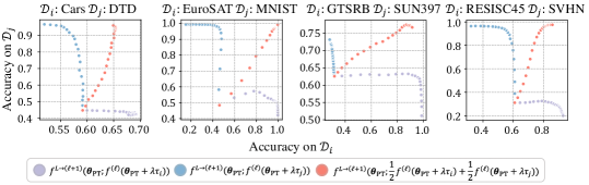
Figure 9: Accuracy of $f^{L\leftarrow(\ell+1)}(\boldsymbol{\theta}_{\rm PT};\frac{1}{2}f^{(\ell)}(\boldsymbol{\theta}_{\rm PT}+\lambda\tau_{i})+\frac{1}{2}f^{(\ell)}(\boldsymbol{\theta}_{\rm PT}+\lambda\tau_{j}))$, $f^{L\leftarrow(\ell+1)}(\boldsymbol{\theta}_{\rm PT};f^{(\ell)}(\boldsymbol{\theta}_{\rm PT}+\lambda\tau_{i}))$ and $f^{L\leftarrow(\ell+1)}(\boldsymbol{\theta}_{\rm PT};f^{(\ell)}(\boldsymbol{\theta}_{\rm PT}+\lambda\tau_{j}))$ on both $\mathcal{D}_{i}$ (x-axis) and $\mathcal{D}_{j}$ (y-axis). Results are reported for ViT-B/32 with various combinations of task vectors and different values of $\lambda\in[0.05,1]$. The stitching layers $\ell$ is chosen to be Block-$9$.

Though Equation 2 has transformed the addition from the parameter space to the feature space, the reason why addition in the feature space constructs multi-task models remains unclear. In fact, we discover that if we replace the features in the pretrained model by the average of the features in two finetuned model, i.e., $f^{L\leftarrow(\ell+1)}(\boldsymbol{\theta}_{\rm PT};\frac{1}{2}f^{(\ell)}(\boldsymbol{\theta}_{i})+\frac{1}{2}f^{(\ell)}(\boldsymbol{\theta}_{j}))$, the model with replaced features could demonstrate abilities on both $\mathcal{D}_{i}$ and $\mathcal{D}_{j}$. Here, $f^{L\leftarrow(\ell+1)}(\boldsymbol{\theta};\cdot)$ denotes the mapping from the internal features of the network $f(\boldsymbol{\theta})$ at $\ell$-th layer to the final output. This feature replacement shares a similar methodology with the model stitching, and thus, we term the model with replaced features as the stitched model. In Figure 9, across various combinations of $\tau_{i}$ and $\tau_{j}$ and different values of $\lambda$, the stitched model $f^{L\leftarrow(\ell+1)}(\boldsymbol{\theta}_{\rm PT};\frac{1}{2}f^{(\ell)}(\boldsymbol{\theta}_{\rm PT}+\lambda\tau_{i})+\frac{1}{2}f^{(\ell)}(\boldsymbol{\theta}_{\rm PT}+\lambda\tau_{j}))$ achieves comparable performance on both $\mathcal{D}_{i}$ and $\mathcal{D}_{j}$, while $f^{L\leftarrow(\ell+1)}(\boldsymbol{\theta}_{\rm PT};f^{(\ell)}(\boldsymbol{\theta}_{\rm PT}+\lambda\tau_{i}))$ and $f^{L\leftarrow(\ell+1)}(\boldsymbol{\theta}_{\rm PT};f^{(\ell)}(\boldsymbol{\theta}_{\rm PT}+\lambda\tau_{j}))$ are only capable of single tasks. Therefore, we conclude that the addition in the feature space actually aggregates the task-specific information from both tasks, thereby bridging the multi-task abilities and CTL.

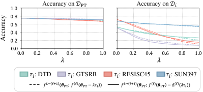
Figure 10: Accuracy of $f^{L\to(\ell+1)}(\boldsymbol{\theta}_{\rm PT};f^{(\ell)}(\boldsymbol{\theta}_{\rm PT})-\Delta^{(\ell)}(\lambda\tau_{i}))$ and $f^{L\to(\ell+1)}(\boldsymbol{\theta}_{\rm PT};f^{(\ell)}(\boldsymbol{\theta}_{\rm PT}-\lambda\tau_{i}))$ on $\mathcal{D}_{\rm PT}$ and $\mathcal{D}_{i}$ v.s. $\lambda$. Results are reported for ViT-L/14 with different task vectors. The stitching layer $\ell$ is chosen to be Block-$19$.

CTL Explains Forgetting via Negation. Another surprising finding in task arithmetic is that negating a task vector removes the ability of the pretrained model on the corresponding task. Specifically, the edited model $f(\boldsymbol{\theta}_{\rm PT}-\lambda\tau_{i})$ forgets its proficiency on $\mathcal{D}_{i}$ while maintaining its performance elsewhere. Further exploration of the underlying reasons for this forgetting effect is encouraged.

We still explain the negation operation from a feature-learning perspective. Assume CTL satisfied for the edited models, we can simply obtain that, $\forall\ell\in[L]$,

$$\small\begin{split}f^{(\ell)}\left(\boldsymbol{\theta}_{\rm PT}\right)\approx\frac{1}{2}f^{(\ell)}(\boldsymbol{\theta}_{\rm PT}+\lambda\tau_{i})+\frac{1}{2}f^{(\ell)}(\boldsymbol{\theta}_{\rm PT}-\lambda\tau_{i}).\end{split}$$ (3)

To verify Equation 3, given a task vector $\tau_{i}$, on each datapoint $\boldsymbol{x}\in\mathcal{D}_{i}$, we measure ${\rm cosine}_{arith}^{(\ell)}(\boldsymbol{x};\lambda\tau_{i},-\lambda\tau_{i})$ and compare it with ${\rm cosine}_{base}^{(\ell)}(\boldsymbol{x};\lambda\tau_{i},-\lambda\tau_{i})$. We also compute ${\rm coef}_{arith}^{(\ell)}(\boldsymbol{x};\lambda\tau_{i},-\lambda\tau_{i})$. The results in Figures 7 and 8 validate our hypothesis in Equation 3.

Equation 3 interprets the negation in the parameter space as the negation in the feature space, as can be rewritten as:

$$\begin{split}f^{(\ell)}\left(\boldsymbol{\theta}_{\rm PT}-\lambda\tau_{i}\right)\approx f^{(\ell)}\left(\boldsymbol{\theta}_{\rm PT}\right)-\Delta^{(\ell)}(\lambda\tau_{i}),\end{split}$$ (4)

where $\Delta^{(\ell)}(\lambda\tau_{i})=f^{(\ell)}\left(\boldsymbol{\theta}_{\rm PT}+\lambda\tau_{i}\right)-f^{(\ell)}\left(\boldsymbol{\theta}_{\rm PT}\right)$. Intuitively, $\Delta^{(\ell)}(\lambda\tau_{i})$ encodes the extra information specific to the task $\mathcal{D}_{i}$. Therefore, $f^{(\ell)}\left(\boldsymbol{\theta}_{\rm PT}-\lambda\tau_{i}\right)$ loses the task-specific information of $\Delta^{(\ell)}(\lambda\tau_{i})$, while retaining most information of $f^{(\ell)}\left(\boldsymbol{\theta}_{\rm PT}\right)$.

We now examine the ability of the negation in the feature space through model stitching. Specifically, we measure the accuracy of the stitched model $f^{L\leftarrow(\ell+1)}(\boldsymbol{\theta}_{\rm PT};f^{(\ell)}(\boldsymbol{\theta}_{\rm PT})-\Delta^{(\ell)}(\lambda\tau_{i}))$ on the downstream task $\mathcal{D}_{i}$ and the pretraining task $\mathcal{D}_{\rm PT}$. In Figure 10, with the increase of $\lambda$, the accuracy of $f^{L\leftarrow(\ell+1)}(\boldsymbol{\theta}_{\rm PT};f^{(\ell)}(\boldsymbol{\theta}_{\rm PT})-\Delta^{(\ell)}(\lambda\tau_{i}))$ drops significantly on $\mathcal{D}_{i}$ while keeping nearly constant on $\mathcal{D}_{\rm PT}$. We also evaluate $f^{L\leftarrow(\ell+1)}(\boldsymbol{\theta}_{\rm PT};f^{(\ell)}(\boldsymbol{\theta}_{\rm PT}-\lambda\tau_{i}))$, which shows a similar performance to $f^{L\leftarrow(\ell+1)}(\boldsymbol{\theta}_{\rm PT};f^{(\ell)}(\boldsymbol{\theta}_{\rm PT})-\Delta^{(\ell)}(\lambda\tau_{i}))$ on both tasks, thus further validating Equation 4. In conclusion, CTL translates the negation in the parameter space as the negation in the feature space, which further induces the aforementioned forgetting effect.

5 Unveiling the Underlying Factors of CTL

We have seen CTL consistently occurs in the pretraining-finetuning paradigm, characterizing networks as linear maps from the parameter space to the feature space. To unveil the root cause of CTL, we investigate the impact of pretraining and take a theoretical attempt to prove CTL.

Impact of Pretraining on CTL. As both spawning method and finetuning require updating model from a common pretrained checkpoint, pretraining plays a crucial role in the emergence of CTL. However, it is not well understood that why pretraining is important. We conceptually conjecture that the common knowledge acquired from the pretraining stage contributes to the satisfaction of CTL. To test our conjecture, we examine the satisfaction of CTL in two cases (see experiments in Section B.3):

i) W/o Pretraining. Independently training two models on different tasks from scratch. We observe the two models struggle to satisfy CTL even after aligning the neurons of two models with permutation [51, 9, 2] (see Figure 11).

ii) W/ Pretraining, W/o Common Knowledge. Pretraining on a random task (with randomly shuffled labels) and then finetuning on different tasks. In this case, where no knowledge is learned from the pretraining stage, CTL may not hold as well (see Figure 12).

This primary step to understand the emergence of CTL emphasizes the role of pretraining. It highlights that acquiring common knowledge through pretraining is crucial to guarantee the satisfaction of CTL.

Theoretical Attempt on CTL. In addition to conceptual understandings, we prove that the emergence of CTL is related to the flatness of the landscape of $f(\cdot)$ and the distance between two finetuned models (see Theorem 1), aligning with previous studies on the contributing factors of LMC [14, 12, 11]. Furthermore, we empirically show a strong correlation between $\delta_{i,j}$ and $\frac{\alpha(1-\alpha)\lambda_{\text{max}}}{2}\left\lVert\boldsymbol{\theta}_{i}-\boldsymbol{\theta}_{j}\right\rVert^{2}$, thereby affirming our theorem in practice (Results in Section B.2).

Theorem 1 (The Emergence of CTL (Proof in Section A.3)).

Suppose $f(\boldsymbol{\theta}):\mathbb{R}^{p}\mapsto\mathbb{R}$ is third differentiable in an open convex set $\boldsymbol{\Theta}$ and the its Hessian norm at $\boldsymbol{\theta}_{0}$ is bounded by $\lambda_{\text{min}}\leq\left\lVert\nabla^{2}f(\boldsymbol{\theta}_{0})\right\rVert\leq\lambda_{\text{max}}$, then

$$\small\begin{split}&\delta_{i,j}=\left\lvert f(\alpha\boldsymbol{\theta}_{i}+(1-\alpha)\boldsymbol{\theta}_{j})-\alpha f(\boldsymbol{\theta}_{i})-(1-\alpha)f(\boldsymbol{\theta}_{j})\right\rvert\\ \leq&\frac{\alpha(1-\alpha)\lambda_{\text{max}}}{2}\left\lVert\boldsymbol{\theta}_{i}-\boldsymbol{\theta}_{j}\right\rVert^{2}+\mathcal{E},\end{split}$$

where $\mathcal{E}=O\left(\max\left(\left\lVert\alpha\boldsymbol{\theta}_{i}+(1-\alpha)\boldsymbol{\theta}_{j}-\boldsymbol{\theta}_{0}\right\rVert^{3},\alpha\left\lVert\boldsymbol{\theta}_{i}-\boldsymbol{\theta}_{0}\right\rVert^{3},\right.\right.$ $\left.\left.(1-\alpha)\left\lVert\boldsymbol{\theta}_{j}-\boldsymbol{\theta}_{0}\right\rVert^{3}\right)\right)$ is the high order term.

Remark 2.

Previous studies found linearizing models is insufficient to explain LMC/LLFC and task arithmetic [12, 44]. In Theorem 1, instead of linearizing models, we provide a more realistic setting. Additionally, it is worth noting that Theorem 1 doesn’t strictly require $\boldsymbol{\theta}_{i}$ and $\boldsymbol{\theta}_{j}$ to be extremely close for LLFC to hold true, as $\delta_{i,j}$ is also bounded by the sharpness of the landscape of $f(\cdot)$, i.e., $\lambda_{\text{max}}$.

6 Conclusion and Limitations

In this work, we identified Cross-Task Linearity (CTL) as a prevalent phenomenon that consistently occurs for finetuned models, approximately characterizing neural networks as linear maps in the pretraining-finetuning paradigm. Based on the observed CTL, we obtained novel insights into two widely-used model merging/editing techniques: model averaging and task arithmetic. Furthermore, we studied the root cause of CTL and highlighted the impact of pretraining.

Similar to recent efforts [63] in the neural network linearity discovery, our current work primarily focuses on empirical findings, despite a limited theoretical attempt to prove CTL in Section 5. We defer a thorough theoretical analysis to future work. Additionally, on the practical side, due to constraints in computational resources, we leave the exploration of CTL on Large Language Models to future.

Appendix A Missing Proofs

A.1 Proof of Lemma 1

Lemma 1 (LLFC Induces LMC).

Given dataset $\mathcal{D}$, convex loss function $L$, and two modes ${\boldsymbol{\theta}}_{i}$ and ${\boldsymbol{\theta}}_{j}$ with equal loss on $\mathcal{D}$, i.e., $\mathcal{L}({\boldsymbol{\theta}}_{i})=\mathcal{L}({\boldsymbol{\theta}}_{j})$, suppose the two modes ${\boldsymbol{\theta}}_{i}$, ${\boldsymbol{\theta}}_{j}$ satisfy LLFC on $\mathcal{D}$ with exact equality, then for all $\alpha\in[0,1]$,

$$\mathcal{L}(\alpha{\boldsymbol{\theta}}_{i}+(1-\alpha){\boldsymbol{\theta}}_{j})\leq\mathcal{L}(\boldsymbol{\theta}_{i})=\mathcal{L}(\boldsymbol{\theta}_{j}).$$

Proof.

Since $\boldsymbol{\theta}_{i}$ and $\boldsymbol{\theta}_{j}$ satisfy LLFC on $\mathcal{D}$ with exact equality, we have

$$f\left(\alpha\boldsymbol{\theta}_{i}+\left(1-\alpha\right)\boldsymbol{\theta}_{j};\boldsymbol{x}\right)=\alpha f\left(\boldsymbol{\theta}_{i};\boldsymbol{x}\right)+\left(1-\alpha\right)f\left(\boldsymbol{\theta}_{j};\boldsymbol{x}\right),\quad\forall\boldsymbol{x}\in\mathcal{D}.$$

Since the loss function $L$ is convex to model outputs, we have

$$L\left(f\left(\alpha\boldsymbol{\theta}_{i}+\left(1-\alpha\right)\boldsymbol{\theta}_{j};\boldsymbol{x}\right),y\right) =L\left(\alpha f\left(\boldsymbol{\theta}_{i};\boldsymbol{x}\right)+\left(1-\alpha\right)f\left(\boldsymbol{\theta}_{j};\boldsymbol{x}\right),y\right)$$

$$\leq\alpha L\left(f\left(\boldsymbol{\theta}_{i};\boldsymbol{x}\right),y\right)+\left(1-\alpha\right)L\left(f\left(\boldsymbol{\theta}_{j};\boldsymbol{x}\right),y\right),\quad\forall(\boldsymbol{x},y)\in\mathcal{D}.$$

Therefore,

$$\mathbb{E}_{(\boldsymbol{x},y)\in\mathcal{D}}\left[L\left(f\left(\alpha\boldsymbol{\theta}_{i}+\left(1-\alpha\right)\boldsymbol{\theta}_{j};\boldsymbol{x}\right),y\right)\right] \leq\mathbb{E}_{(\boldsymbol{x},y)\in\mathcal{D}}\left[\alpha L\left(f\left(\boldsymbol{\theta}_{i};\boldsymbol{x}\right),y\right)\right]+\mathbb{E}_{(\boldsymbol{x},y)\in\mathcal{D}}\left[\left(1-\alpha\right)L\left(f\left(\boldsymbol{\theta}_{j};\boldsymbol{x}\right),y\right)\right]$$

$$\mathcal{L}\left(\alpha{\boldsymbol{\theta}}_{i}+(1-\alpha){\boldsymbol{\theta}}_{j}\right) \leq\alpha\mathcal{L}(\boldsymbol{\theta}_{i})+\left(1-\alpha\right)\mathcal{L}(\boldsymbol{\theta}_{j})$$

According to the condition that $\mathcal{L}(\boldsymbol{\theta}_{i})=\mathcal{L}(\boldsymbol{\theta}_{j})$, we finally obtain that

$$\mathcal{L}(\alpha{\boldsymbol{\theta}}_{i}+(1-\alpha){\boldsymbol{\theta}}_{j})\leq\mathcal{L}(\boldsymbol{\theta}_{i})=\mathcal{L}(\boldsymbol{\theta}_{j}).$$

∎

A.2 Proof of Lemma 2

Lemma 2 (CTL Generalizes to Multiple Models).

Given dataset $\mathcal{D}$ and a field of modes $\boldsymbol{\Theta}$ where each pair of modes $(\boldsymbol{\theta}_{i},\boldsymbol{\theta}_{j})\in\boldsymbol{\Theta}^{2}$ satisfy CTL on $\mathcal{D}$, then for any $\{\boldsymbol{\theta}_{i}\}_{i=1}^{k}\in\boldsymbol{\Theta}$ and $\{\alpha_{i}\}_{i=1}^{k}\in[0,1]$, subject to the constraint that $\sum_{i=1}^{k}\alpha_{i}=1$, we have

$$f^{(\ell)}\left(\sum_{i=1}^{k}\alpha_{i}\boldsymbol{\theta}_{i}\right)\approx\sum_{i=1}^{k}\alpha_{i}f^{(\ell)}({\boldsymbol{\theta}}_{i}),\quad\forall\ell\in[L].$$

Proof.

We proceed by induction on $k$. When $k=2$, Lemma 2 clearly holds. For any $(\boldsymbol{\theta}_{1},\boldsymbol{\theta}_{2})\in\boldsymbol{\Theta}^{2}$, CTL holds on $\mathcal{D}$. Then, $\forall\alpha_{1}\in[0,1]$ and $\alpha_{2}=1-\alpha_{1}\in[0,1]$, we have

$$f^{(\ell)}(\alpha_{1}\boldsymbol{\theta}_{1}+\alpha_{2}\boldsymbol{\theta}_{2}) =f^{(\ell)}\left(\sum_{i=1}^{2}\alpha_{i}\boldsymbol{\theta}_{i}\right)$$

$$\approx\alpha_{1}f^{(\ell)}(\boldsymbol{\theta}_{1})+\alpha_{2}f^{(\ell)}(\boldsymbol{\theta}_{2})$$

$$\approx\sum_{i=1}^{2}\alpha_{i}f^{(\ell)}(\boldsymbol{\theta}_{i}),\quad\forall\ell\in[L].$$

Assume Lemma 2 holds for some $k^{\prime}\geq 2$. That is, assume that for any $\{\boldsymbol{\theta}_{i}\}_{i=1}^{k^{\prime}}\in\boldsymbol{\Theta}$ and $\{\alpha_{i}\}_{i=1}^{k^{\prime}}\in[0,1]$, subject to the constraint that $\sum_{i=1}^{k^{\prime}}\alpha_{i}=1$, we have

$$f^{(\ell)}\left(\sum_{i=1}^{k^{\prime}}\alpha_{i}\boldsymbol{\theta}_{i}\right)\approx\sum_{i=1}^{k^{\prime}}\alpha_{i}f^{(\ell)}({\boldsymbol{\theta}}_{i}),\quad\forall\ell\in[L].$$

Now we need to show Lemma 2 holds when $k=k^{\prime}+1$. For any set of modes $\{\boldsymbol{\theta}_{i}\}_{i=1}^{k^{\prime}+1}\in\boldsymbol{\Theta}$ and any set of coefficients $\{\alpha_{i}\}_{i=1}^{k^{\prime}+1}\in[0,1]$, we define $\boldsymbol{\theta}_{avg,k^{\prime}}=\sum_{i=1}^{k^{\prime}}\frac{\alpha_{i}}{1-\alpha_{k^{\prime}+1}}\boldsymbol{\theta}_{i}\in\boldsymbol{\Theta}$. As CTL holds for each pair of modes from $\boldsymbol{\Theta}^{2}$, then we have

$$f^{(\ell)}(\alpha\boldsymbol{\theta}_{k^{\prime}+1}+(1-\alpha)\boldsymbol{\theta}_{avg,k^{\prime}})\approx\alpha f^{(\ell)}(\boldsymbol{\theta}_{k^{\prime}+1})+(1-\alpha)f^{(\ell)}(\boldsymbol{\theta}_{avg,k^{\prime}}),\quad\forall\alpha\in[0,1],\forall\ell\in[L].$$

Substituting $\alpha$ with $\alpha_{k^{\prime}+1}$, we can obtain $\forall\alpha\in[0,1],\forall\ell\in[L]$,

$$f^{(\ell)}(\alpha_{k^{\prime}+1}\boldsymbol{\theta}_{k^{\prime}+1}+(1-\alpha_{k^{\prime}+1})\boldsymbol{\theta}_{avg,k^{\prime}}) =f^{(\ell)}\left(\sum_{i=1}^{k^{\prime}+1}\alpha_{i}\boldsymbol{\theta}_{i}\right)$$

$$\approx\alpha_{k^{\prime}+1}f^{(\ell)}(\boldsymbol{\theta}_{k^{\prime}+1})+(1-\alpha_{k^{\prime}+1})f^{(\ell)}(\boldsymbol{\theta}_{avg,k^{\prime}}).$$

Knowing that Lemma 2 holds true when $k=k^{\prime}$, then we have

$$f^{(\ell)}\left(\sum_{i=1}^{k^{\prime}+1}\alpha_{i}\boldsymbol{\theta}_{i}\right) \approx\alpha_{k^{\prime}+1}f^{(\ell)}(\boldsymbol{\theta}_{k^{\prime}+1})+(1-\alpha_{k^{\prime}+1})f^{(\ell)}\left(\sum_{i=1}^{k^{\prime}}\frac{\alpha_{i}}{1-\alpha_{k^{\prime}+1}}\boldsymbol{\theta}_{i}\right)$$

$$\approx\alpha_{k^{\prime}+1}f^{(\ell)}(\boldsymbol{\theta}_{k^{\prime}+1})+(1-\alpha_{k^{\prime}+1})\sum_{i=1}^{k^{\prime}}\frac{\alpha_{i}}{1-\alpha_{k^{\prime}+1}}f^{(\ell)}(\boldsymbol{\theta}_{i})$$

$$\approx\sum_{i=1}^{k^{\prime}+1}\alpha_{i}f^{(\ell)}({\boldsymbol{\theta}}_{i}),\quad\forall\ell\in[L].$$

Therefore, Lemma 2 holds true when $k=k^{\prime}+1$, and this finishes our proof. ∎

A.3 Proof of Theorem 1

Theorem 1 (The Emergence of CTL).

Suppose $f(\boldsymbol{\theta}):\mathbb{R}^{p}\mapsto\mathbb{R}$ is third differentiable in an open convex set $\boldsymbol{\Theta}$ and the its Hessian norm at $\boldsymbol{\theta}_{0}$ is bounded by $\lambda_{\text{min}}\leq\left\lVert\nabla^{2}f(\boldsymbol{\theta}_{0})\right\rVert\leq\lambda_{\text{max}}$, then

$$\delta_{i,j}=\left\lvert f(\alpha\boldsymbol{\theta}_{i}+(1-\alpha)\boldsymbol{\theta}_{j})-\alpha f(\boldsymbol{\theta}_{i})-(1-\alpha)f(\boldsymbol{\theta}_{j})\right\rvert\leq\frac{\alpha(1-\alpha)\lambda_{\text{max}}}{2}\left\lVert\boldsymbol{\theta}_{j}-\boldsymbol{\theta}_{i}\right\rVert^{2}+\mathcal{E},$$

where $\mathcal{E}=O\left(\max\left(\left\lVert\alpha\boldsymbol{\theta}_{i}+(1-\alpha)\boldsymbol{\theta}_{j}-\boldsymbol{\theta}_{0}\right\rVert^{3},\alpha\left\lVert\boldsymbol{\theta}_{i}-\boldsymbol{\theta}_{0}\right\rVert^{3},(1-\alpha)\left\lVert\boldsymbol{\theta}_{j}-\boldsymbol{\theta}_{0}\right\rVert^{3}\right)\right)$ is the high order term.

Proof.

Since $f$ is third differentiable in an open convex set $\boldsymbol{\Theta}$, then by Taylor’s Theorem, for any $\boldsymbol{\theta}_{0},\boldsymbol{\theta}\in\boldsymbol{\Theta}$,

$$f(\boldsymbol{\theta})=f(\boldsymbol{\theta}_{0})+\nabla f(\boldsymbol{\theta}_{0})^{\top}\left(\boldsymbol{\theta}-\boldsymbol{\theta}_{0}\right)+\frac{1}{2}\left(\boldsymbol{\theta}-\boldsymbol{\theta}_{0}\right)^{\top}\nabla^{2}f(\boldsymbol{\theta}_{0})\left(\boldsymbol{\theta}-\boldsymbol{\theta}_{0}\right)+R_{\boldsymbol{\theta}_{0},3}(\boldsymbol{\theta}-\boldsymbol{\theta}_{0}).$$

where the remainder term $R_{\boldsymbol{\theta}_{0},3}(\boldsymbol{\theta}-\boldsymbol{\theta}_{0})=O\left(\left\lVert\boldsymbol{\theta}-\boldsymbol{\theta}_{0}\right\rVert^{3}\right)$. Suppose $\lambda_{\text{min}}\leq\left\lVert\nabla^{2}f(\boldsymbol{\theta}_{0})\right\rVert\leq\lambda_{\text{max}}$, we have

$$\frac{\lambda_{\text{min}}}{2}\left\lVert\boldsymbol{\theta}-\boldsymbol{\theta}_{0}\right\rVert^{2}\leq\frac{1}{2}\left(\boldsymbol{\theta}-\boldsymbol{\theta}_{0}\right)^{\top}\nabla^{2}f(\boldsymbol{\theta}_{0})\left(\boldsymbol{\theta}-\boldsymbol{\theta}_{0}\right)\leq\frac{\lambda_{\text{max}}}{2}\left\lVert\boldsymbol{\theta}-\boldsymbol{\theta}_{0}\right\rVert^{2}.$$

Then for $f(\alpha\boldsymbol{\theta}_{i}+(1-\alpha)\boldsymbol{\theta}_{j})$, by Taylor’s Theorem,

$$f(\alpha\boldsymbol{\theta}_{i}+(1-\alpha)\boldsymbol{\theta}_{j})$$

$$=f(\boldsymbol{\theta}_{0})+\nabla f(\boldsymbol{\theta}_{0})^{\top}\left(\alpha\boldsymbol{\theta}_{i}+(1-\alpha)\boldsymbol{\theta}_{j}-\boldsymbol{\theta}_{0}\right)$$

$$\quad+\frac{1}{2}\left(\alpha\boldsymbol{\theta}_{i}+(1-\alpha)\boldsymbol{\theta}_{j}-\boldsymbol{\theta}_{0}\right)^{\top}\nabla^{2}f(\boldsymbol{\theta}_{0})\left(\alpha\boldsymbol{\theta}_{i}+(1-\alpha)\boldsymbol{\theta}_{j}-\boldsymbol{\theta}_{0}\right)+R_{\boldsymbol{\theta}_{0},3}(\alpha\boldsymbol{\theta}_{i}+(1-\alpha)\boldsymbol{\theta}_{j}-\boldsymbol{\theta}_{0})$$

$$=f(\boldsymbol{\theta}_{0})+\nabla f(\boldsymbol{\theta}_{0})^{\top}\left(\alpha\left(\boldsymbol{\theta}_{i}-\boldsymbol{\theta}_{0}\right)+(1-\alpha)\left(\boldsymbol{\theta}_{j}-\boldsymbol{\theta}_{0}\right)\right)$$

$$\quad+\frac{1}{2}\left(\alpha\boldsymbol{\theta}_{i}+(1-\alpha)\boldsymbol{\theta}_{j}-\boldsymbol{\theta}_{0}\right)^{\top}\nabla^{2}f(\boldsymbol{\theta}_{0})\left(\alpha\boldsymbol{\theta}_{i}+(1-\alpha)\boldsymbol{\theta}_{j}-\boldsymbol{\theta}_{0}\right)+R_{\boldsymbol{\theta}_{0},3}(\alpha\boldsymbol{\theta}_{i}+(1-\alpha)\boldsymbol{\theta}_{j}-\boldsymbol{\theta}_{0})$$

$$=\alpha\left(f(\boldsymbol{\theta}_{0})+\nabla f(\boldsymbol{\theta}_{0})^{\top}\left(\boldsymbol{\theta}_{i}-\boldsymbol{\theta}_{0}\right)\right)+(1-\alpha)\left(f(\boldsymbol{\theta}_{0})+\nabla f(\boldsymbol{\theta}_{0})^{\top}\left(\boldsymbol{\theta}_{i}-\boldsymbol{\theta}_{0}\right)\right)$$

$$\quad+\frac{1}{2}\left(\alpha\boldsymbol{\theta}_{i}+(1-\alpha)\boldsymbol{\theta}_{j}-\boldsymbol{\theta}_{0}\right)^{\top}\nabla^{2}f(\boldsymbol{\theta}_{0})\left(\alpha\boldsymbol{\theta}_{i}+(1-\alpha)\boldsymbol{\theta}_{j}-\boldsymbol{\theta}_{0}\right)+R_{\boldsymbol{\theta}_{0},3}(\alpha\boldsymbol{\theta}_{i}+(1-\alpha)\boldsymbol{\theta}_{j}-\boldsymbol{\theta}_{0})$$

$$=\alpha\left(f(\boldsymbol{\theta}_{i})-\frac{1}{2}\left(\boldsymbol{\theta}_{i}-\boldsymbol{\theta}_{0}\right)^{\top}\nabla^{2}f(\boldsymbol{\theta}_{0})\left(\boldsymbol{\theta}_{i}-\boldsymbol{\theta}_{0}\right)-R_{\boldsymbol{\theta}_{0},3}(\boldsymbol{\theta}_{i}-\boldsymbol{\theta}_{0})\right)$$

$$\quad+(1-\alpha)\left(f(\boldsymbol{\theta}_{j})-\frac{1}{2}\left(\boldsymbol{\theta}_{j}-\boldsymbol{\theta}_{0}\right)^{\top}\nabla^{2}f(\boldsymbol{\theta}_{0})\left(\boldsymbol{\theta}_{j}-\boldsymbol{\theta}_{0}\right)-R_{\boldsymbol{\theta}_{0},3}(\boldsymbol{\theta}_{j}-\boldsymbol{\theta}_{0})\right)$$

$$\quad+\frac{1}{2}\left(\alpha\boldsymbol{\theta}_{i}+(1-\alpha)\boldsymbol{\theta}_{j}-\boldsymbol{\theta}_{0}\right)^{\top}\nabla^{2}f(\boldsymbol{\theta}_{0})\left(\alpha\boldsymbol{\theta}_{i}+(1-\alpha)\boldsymbol{\theta}_{j}-\boldsymbol{\theta}_{0}\right)+R_{\boldsymbol{\theta}_{0},3}(\alpha\boldsymbol{\theta}_{i}+(1-\alpha)\boldsymbol{\theta}_{j}-\boldsymbol{\theta}_{0})$$

$$=\alpha f(\boldsymbol{\theta}_{i})+(1-\alpha)f(\boldsymbol{\theta}_{j})$$

$$\quad+\frac{1}{2}\left(\alpha\left(\boldsymbol{\theta}_{i}-\boldsymbol{\theta}_{0}\right)+(1-\alpha)\left(\boldsymbol{\theta}_{j}-\boldsymbol{\theta}_{0}\right)\right)^{\top}\nabla^{2}f(\boldsymbol{\theta}_{0})\left(\alpha\left(\boldsymbol{\theta}_{i}-\boldsymbol{\theta}_{0}\right)+(1-\alpha)\left(\boldsymbol{\theta}_{j}-\boldsymbol{\theta}_{0}\right)\right)$$

$$\quad-\frac{\alpha}{2}\left(\boldsymbol{\theta}_{i}-\boldsymbol{\theta}_{0}\right)^{\top}\nabla^{2}f(\boldsymbol{\theta}_{0})\left(\boldsymbol{\theta}_{i}-\boldsymbol{\theta}_{0}\right)-\frac{(1-\alpha)}{2}\left(\boldsymbol{\theta}_{j}-\boldsymbol{\theta}_{0}\right)^{\top}\nabla^{2}f(\boldsymbol{\theta}_{0})\left(\boldsymbol{\theta}_{j}-\boldsymbol{\theta}_{0}\right)$$

$$\quad+R_{\boldsymbol{\theta}_{0},3}(\alpha\boldsymbol{\theta}_{i}+(1-\alpha)\boldsymbol{\theta}_{j}-\boldsymbol{\theta}_{0})-\alpha R_{\boldsymbol{\theta}_{0},3}(\boldsymbol{\theta}_{i}-\boldsymbol{\theta}_{0})-(1-\alpha)R_{\boldsymbol{\theta}_{0},3}(\boldsymbol{\theta}_{j}-\boldsymbol{\theta}_{0})$$

$$=\alpha f(\boldsymbol{\theta}_{i})+(1-\alpha)f(\boldsymbol{\theta}_{j})$$

$$\quad-\frac{\alpha(1-\alpha)}{2}\left(\boldsymbol{\theta}_{j}-\boldsymbol{\theta}_{i}\right)^{\top}\nabla^{2}f(\boldsymbol{\theta}_{0})\left(\boldsymbol{\theta}_{j}-\boldsymbol{\theta}_{i}\right)$$

$$\quad+R_{\boldsymbol{\theta}_{0},3}(\alpha\boldsymbol{\theta}_{i}+(1-\alpha)\boldsymbol{\theta}_{j}-\boldsymbol{\theta}_{0})-\alpha R_{\boldsymbol{\theta}_{0},3}(\boldsymbol{\theta}_{i}-\boldsymbol{\theta}_{0})-(1-\alpha)R_{\boldsymbol{\theta}_{0},3}(\boldsymbol{\theta}_{j}-\boldsymbol{\theta}_{0}).$$

Therefore, we have

$$\quad\left\lvert f(\alpha\boldsymbol{\theta}_{i}+(1-\alpha)\boldsymbol{\theta}_{j})-\alpha f(\boldsymbol{\theta}_{i})-(1-\alpha)f(\boldsymbol{\theta}_{j})\right\rvert$$

$$\leq\left\lvert\frac{\alpha(1-\alpha)}{2}\left(\boldsymbol{\theta}_{j}-\boldsymbol{\theta}_{i}\right)^{\top}\nabla^{2}f(\boldsymbol{\theta}_{0})\left(\boldsymbol{\theta}_{j}-\boldsymbol{\theta}_{i}\right)\right\rvert$$

$$\quad+\left\lvert R_{\boldsymbol{\theta}_{0},3}(\alpha\boldsymbol{\theta}_{i}+(1-\alpha)\boldsymbol{\theta}_{j}-\boldsymbol{\theta}_{0})-\alpha R_{\boldsymbol{\theta}_{0},3}(\boldsymbol{\theta}_{i}-\boldsymbol{\theta}_{0})-(1-\alpha)R_{\boldsymbol{\theta}_{0},3}(\boldsymbol{\theta}_{j}-\boldsymbol{\theta}_{0})\right\rvert$$

$$\leq\frac{\alpha(1-\alpha)\lambda_{\text{max}}}{2}\left\lVert\boldsymbol{\theta}_{j}-\boldsymbol{\theta}_{i}\right\rVert^{2}+O\left(\max\left(\left\lVert\alpha\boldsymbol{\theta}_{i}+(1-\alpha)\boldsymbol{\theta}_{j}-\boldsymbol{\theta}_{0}\right\rVert^{3},\alpha\left\lVert\boldsymbol{\theta}_{i}-\boldsymbol{\theta}_{0}\right\rVert^{3},(1-\alpha)\left\lVert\boldsymbol{\theta}_{j}-\boldsymbol{\theta}_{0}\right\rVert^{3}\right)\right).$$

where the last inequality is because $\lambda_{\text{min}}\leq\left\lVert\nabla^{2}f(\boldsymbol{\theta}_{0})\right\rVert\leq\lambda_{\text{max}}$ and $R_{\boldsymbol{\theta}_{0},3}(\boldsymbol{\theta}-\boldsymbol{\theta}_{0})=O\left(\left\lVert\boldsymbol{\theta}-\boldsymbol{\theta}_{0}\right\rVert^{3}\right)$.

∎

Appendix B More Experimental Results

B.1 Detailed Experimental Settings

B.1.1 Experimental Settings in Section 4.1

Multi-Layer Perceptron on the Rotated MNIST Dataset. Following the settings outlined by Mirzadeh et al. [37], we adopt the multi-layer perceptron with two hidden layers with $100$ units for Rotated MNIST dataset. ReLU activation functions are adopted between linear layers. Therefore, the multi-layer perceptron has $4$ linear layers ($1$ for input, $2$ for hidden and $1$ for output) and $3$ ReLU layers. We pretrain the MLP on normal MNIST and finetune it on Rotated MNIST, where each digit are rotated by a specific angle. We use rotation angle degrees of $\{0^{\circ},22.5^{\circ},45^{\circ},67.5^{\circ},90^{\circ}\}$. Optimization is done with the default SGD algorithm and the learning rate of $1\times 10^{-1}$, the batch size is set to $64$ and the training epoch is set to $1$ for both pretraining and finetuning.

We have $4$ finetuned MLPs, yielding $6$ non-repeated combinations of two finetuned models $(\boldsymbol{\theta}_{i},\boldsymbol{\theta}_{j})$ in total. CTL are evaluated for each combinations on the union of their finetuning tasks ($\mathcal{D}_{i}\cup\mathcal{D}_{j}$) which have $20,000$ test samples.

ResNet-18 on the Split CIFAR-100 Dataset. Still following the settings outlined by Mirzadeh et al. [37], we adopt the ResNet-18 architecture [17] on the Split CIFAR-100 dataset. The Split CIFAR-100 dataset is divided by classes, and $5$ consecutive categories of CIFAR-100 are grouped into one split, having $20$ splits in total. We use the first split as pretraining task and the second to fifth splits as finetuning tasks. We pretrain the ResNet-18 on first split and finetune it on the rest $4$ splits respectively, acquiring 4 finetuned ResNet-18 checkpoints. No data augmentation techniques are adopted and optimization is done using the default SGD algorithm with learning rate of $5\times 10^{-2}$. The batch size is set to $64$. The training epoch is set to 10 for both pretraining and finetuning.

Similar to the setup of the Rotated MNIST experiment, we have $4$ finetuned ResNet-18 models, yielding $6$ non-repeated combinations of two finetuned models $(\boldsymbol{\theta}_{i},\boldsymbol{\theta}_{j})$ in total. CTL are evaluated for each combinations and on the union of their finetuning tasks ($\mathcal{D}_{i}\cup\mathcal{D}_{j}$) which have $20,000$ test samples.

B.1.2 Experimental Settings in Section 4.2

Model Averaging Accuracy v.s. Logits Ensemble Accuracy. We choose $20$ out of the $72$ ViT-B/32 [6] checkpoints that are finetuned on ImageNet and open-sourced by Wortsman et al. [56], yielding $\binom{20}{3}=1140$ non-repeated combinations of three finetuned ViT-B/32 models. For each combination of the finetuned models, we evaluated model averaging accuracy and logits ensemble accuracy on $10,000$ test samples from ImageNet.

Verification of Equation 1. For ViT-B/32 on CIFAR-10, We train our ViT-B/32 initialized from same CLIP pretrained checkpoint but finetuned on CIFAR-10 dataset with different hyper-parameters to obtain $5$ checkpoints to validate Equation 1. For ViT-B/32 on ImageNet, we choose $10$ out of the $72$ ViT-B/32 checkpoints that are finetuned on ImageNet and open-sourced by Wortsman et al. [56] to validate Equation 1. For both cases, we perform experiments on randomly-selected $10,000$ samples from the test set.

It’s worth mentioning that in the forward pass of ViT models, the input in the shape of (batch_size, patches_num, hidden_dim) will be permuted to (patches_num, batch_size, hidden_dim). We permute the internal feature back and reshape it into (batch_size, patches_num $\times$ hidden_dim). Now, the dimension of the features is simply patches_num $\times$ hidden_dim.

B.1.3 Experimental Settings in Section 4.3

CTL Explains Learning via Addition. We present the experimental settings in (i) Cross-Task Linearity (CTL) and (ii) Model Stitching experiment, respectively. In CTL experiment, we evaluate two ViT architectures (ViT-B/32, ViT-L/14) on $8$ image classification datasets: Cars[25], DTD[5], EuroSAT[18], GTSRB[52], MNIST[28], RESISC45[4], SUN397[58], SVHN[39]) and a T5 architecture (T5-base) [47] on $6$ NLP datasets: IMDB[34], RACE[27], QASC[24], MultiNews[10], SQuAD[48], CommonGen[32], as same setup in Ilharco et al. [20]. In Model Stitching experiment, we only validate two ViT architectures (ViT-B/32, ViT-L/14) on the aforementioned $8$ image classification datasets. Notice that instead of training by ourselves, we directly use the finetuned checkpoints are open-sourced by Ilharco et al. [20] for both ViT and T5 models.

For ViT architectures, in CTL experiment, $8$ finetuned ViT-B/32 (ViT-L/14) models generate $\binom{8}{2}=28$ non-repeated combinations of two task vectors in total. For each combination of the two task vectors, we validate Equation 2 on on the union of their finetuning datasets ($\mathcal{D}_{i}\cup\mathcal{D}_{j}$) which has $10,000$ test samples in total. In Model Stitching experiment, we follow the above settings except for the evaluation data size, which is of $2,000$ in this case. Notably, it is impossible for us to include the results for all $28$ combinations, and thus, part of our experimental results will be presented, which is the same for the other experiments. For T5 architectures, in CTL experiment, $6$ finetuned T5-base models generate $\binom{6}{2}=15$ non-repeated combinations of two task vectors in total. For each combination of the two task vectors, we validate Equation 2 on on the union of their finetuning datasets ($\mathcal{D}_{i}\cup\mathcal{D}_{j}$) which has $1,000$ test samples in total.

As T5 is a encoder-decoder architecture and sentences are varied in their lengths, we adopt the convention in sentence-T5 [42], which uses (i) the average pooling of tokens in the encoder to represent the internal feature of a sentence and (ii) the decoder’s hidden states when generating first token (which is equivalent to attention pooling) to represent the feature of a sentence in decoder.

CTL Explains Learning via Negation. Similar to the Addition setup, the datasets and architectures are kept the same. In CTL experiment, we evaluate both ViT and T5 architectures, while in Model Stitching experiment, we only validate ViT architectures.

For ViT architectures, in CTL experiment, we evaluate the $8$ finetuned models on their corresponding datasets, each having $10,000$ test samples. In Model Stitching experiment, we follow the same settings as above except for evaluation data size, which is of $2,000$ in this case. While for T5 architectures, in CTL experiment, we evaluate the $6$ finetuned models on their corresponding datasets, each having $10,000$ test samples.

B.2 Verification of Theorem 1

In this section, we conduct experiments to validate the theoretical analysis presented in Theorem 1. Specifically, we demonstrate that $\delta_{i,j}$ exhibits a stronger correlation with $\frac{\alpha(1-\alpha)\lambda_{\text{max}}}{2}\left\lVert\boldsymbol{\theta}_{i}-\boldsymbol{\theta}_{j}\right\rVert^{2}$ compared to $\lambda_{\text{max}}$ or $\left\lVert\boldsymbol{\theta}_{i}-\boldsymbol{\theta}_{j}\right\rVert^{2}$ alone.

For each pair of $\boldsymbol{\theta}_{i}$ and $\boldsymbol{\theta}_{j}$, we calculate the distance between finetuned models, i.e., $\left\lVert\boldsymbol{\theta}_{i}-\boldsymbol{\theta}_{j}\right\rVert^{2}$, and $\delta_{i,j}$, i.e., $|f(\alpha\boldsymbol{\theta}_{i}+(1-\alpha)\boldsymbol{\theta}_{j})-\alpha f(\boldsymbol{\theta}_{i})-(1-\alpha)f(\boldsymbol{\theta}_{j})|$ where $\alpha=0.5$. We also compute the largest eigenvalue of the Hessian matrix of $f(\cdot)$ at $\boldsymbol{\theta}_{0}$, i.e., $\lambda_{\rm max}$. Here, $\boldsymbol{\theta}_{i}$ and $\boldsymbol{\theta}_{j}$ denote models that are initialized from a common checkpoint and finetuned on the same dataset with different hyperparameters. The function $f(\cdot)$ represents the loss function $\mathcal{L}(\cdot)$, and $\boldsymbol{\theta}_{0}$ is simply chosen as $\boldsymbol{\theta}_{\rm PT}$.

For ResNet-20 models finetuned on the CIFAR-10 dataset, we find that if we use $\frac{\alpha(1-\alpha)\lambda_{\text{max}}}{2}\left\lVert\boldsymbol{\theta}_{i}-\boldsymbol{\theta}_{j}\right\rVert^{2}$ to fit a regression model to predict $\delta_{i,j}$, the R-squared value of the model is approximately $0.903$. However, if we use only $\lambda_{\text{max}}$ or $\left\lVert\boldsymbol{\theta}_{i}-\boldsymbol{\theta}_{j}\right\rVert^{2}$ to fit the regression model, the R-squared value of the model is approximately $0.782$ or $0.839$, respectively. Therefore, we conclude that $\delta_{i,j}$ indeed demonstrates a strong correlation with $\frac{\alpha(1-\alpha)\lambda_{\text{max}}}{2}\left\lVert\boldsymbol{\theta}_{i}-\boldsymbol{\theta}_{j}\right\rVert^{2}$. It is worth noting that such correlation is a joint effect of both $\lambda_{\text{max}}$ and $\left\lVert\boldsymbol{\theta}_{i}-\boldsymbol{\theta}_{j}\right\rVert^{2}$, implying that either reducing $\lambda_{\text{max}}$ or $\left\lVert\boldsymbol{\theta}_{i}-\boldsymbol{\theta}_{j}\right\rVert^{2}$ leads to the fulfillment of CTL.

B.3 Verification of the Role of Pretraining

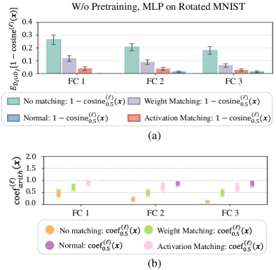
Figure 11: (a) Compare $\mathbb{E}_{\mathcal{D}}[1-{\rm cosine}_{0.5}^{(\ell)}(\boldsymbol{x})]$ among four settings in each layer: (1) No Matching (2) Weight Matching (3) Activation Matching (4) Normal Pretraining-Finetuning Paradigm. The bottom and top of the error bar represent the lower and upper quartile of the values across the dataset, respectively. (b) Distribution of $\text{coef}_{0.5}^{(\ell)}(\boldsymbol{x})$ across the above four settings. We use the Rotated MNIST with angles of $45^{\circ}$ and $90^{\circ}$ as finetuning tasks. All linear layers except the last linear classification head are reported.

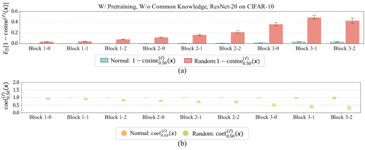
Figure 12: (a) Compare $\mathbb{E}_{\mathcal{D}}[1-{\rm cosine}_{0.5}^{(\ell)}(\boldsymbol{x})]$ among two settings: (1) Random Label Pretraining (2) Normal Pretraining-Finetuning Paradigm. The bottom and top of the error bar represent the lower and upper quartile of the values across the dataset, respectively. (b) Distribution of $\text{coef}_{0.5}^{(\ell)}(\boldsymbol{x})$ across the above two settings. We report all the blocks of ResNet-20.

i) W/o Pretraining. In this part, we try to investigate the satisfaction of CTL for models that shares no pretraining stage. Specifically, we have two pair of models: 1) normal: the models that are initialized from a same pretrained checkpoint and finetuned on different datasets; 2) No matching: the models that are completely trained on the different datasets. It is apparent that two completely independent trained networks may not satisfy CTL due to the complex non-linear nature of neural networks. However, recent studies [9, 2] found even completely independently trained neural networks can satisfy LMC after aligning the neurons of two networks with permutations. Therefore, we employ the two approaches proposed by Ainsworth et al. [2], the weight matching and the activation matching, to align the neurons of models that are completely trained on the different datasets, i.e., the second pair. Thus, we have two more pairs: 3) weight matching: the models that are completely trained on the different datasets but applied with weight matching; 4) activation matching: the models that are completely trained on the different datasets but applied with activation matching. To verify CTL, for each pair of models $\boldsymbol{\theta}_{i}$ and $\boldsymbol{\theta}_{j}$, on each datapoint $\boldsymbol{x}$ from the dataset for finetuning $\mathcal{D}$, we measure $\text{cosine}_{0.5}^{(\ell)}(\boldsymbol{x})=\cos[f^{(\ell)}(\frac{1}{2}\boldsymbol{\theta}_{i}+\frac{1}{2}\boldsymbol{\theta}_{j};\boldsymbol{x}),\frac{1}{2}f^{(\ell)}(\boldsymbol{\theta}_{i};\boldsymbol{x})+\frac{1}{2}f^{(\ell)}(\boldsymbol{\theta}_{j};\boldsymbol{x})]$ and ${\rm coef}_{0.5}^{(\ell)}(\boldsymbol{x})=\frac{\|f^{(\ell)}(\frac{1}{2}\boldsymbol{\theta}_{i}+\frac{1}{2}\boldsymbol{\theta}_{j};\boldsymbol{x})\|\text{\ cosine}_{0.5}^{(\ell)}(\boldsymbol{x})}{\|\frac{1}{2}f^{(\ell)}(\boldsymbol{\theta}_{i};\boldsymbol{x})+\frac{1}{2}f^{(\ell)}(\boldsymbol{\theta}_{j};\boldsymbol{x})\|}$ at each layer $\ell$. In Figure 11, the values of $\mathbb{E}_{\mathcal{D}}[1-{\rm cosine}_{0.5}^{(\ell)}(\boldsymbol{x})]$ for the models without pretraining stage are not close $0$ compared to those values for the models with pretraining. Though the values of $\mathbb{E}_{\mathcal{D}}[1-{\rm cosine}_{0.5}^{(\ell)}(\boldsymbol{x})]$ for models without pretraining is closer to $0$ after weight matching and activation matching, they are still larger than those values for the models with pretraining. Additionally, for models without pretraining, the values of $\mathbb{E}_{\mathcal{D}}[1-{\rm coef}_{0.5}^{(\ell)}(\boldsymbol{x})]$ also deviate from $1$. Therefore, we conclude that the pretraining stage is essential for the satisfaction of CTL.

ii) W/ Pretraining, W/o Common Knowledge. Taking a step further, we try to investigate the satisfaction of CTL for the finetuned models that learn no knowledge from the pretraining stage. Specifically, we have two pair of models: 1)normal: the models that start from a same normally pretrained checkpoint and are finetuned on the same dataset with different hyperparameters; 2) random: the models that start from a same randomly pretrained checkpoint (the labels for the pretraining task are randomly shuffled) and are finetuned on the same dataset with different hyperparameters. Similar as before, to verify CTL, for each pair of models $\boldsymbol{\theta}_{i}$ and $\boldsymbol{\theta}_{j}$, on each datapoint $\boldsymbol{x}$ from the dataset for finetuning $\mathcal{D}$, we measure $\text{cosine}_{0.5}^{(\ell)}(\boldsymbol{x})$ and ${\rm coef}_{0.5}^{(\ell)}(\boldsymbol{x})$ at each layer $\ell$. In Figure 12, the values of $\mathbb{E}_{\mathcal{D}}[1-{\rm cosine}_{0.5}^{(\ell)}(\boldsymbol{x})]$ for the models that are pretrained randomly stronger are far from $0$ compared to those values for the models that are pretrained normally. The values of $\mathbb{E}_{\mathcal{D}}[1-{\rm coef}_{0.5}^{(\ell)}(\boldsymbol{x})]$ for models pretrained randomly also deviate from $1$. Therefore, we conclude that even with pretraining, if no common knowledge learned from the pretraining stage, CTL still may not holds well.

B.4 More Verification of CTL

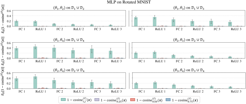
Figure 13: Compare $\mathbb{E}_{\mathcal{D}}[1-{\rm cosine}_{\alpha}^{(\ell)}(\boldsymbol{x})]$ with $\mathbb{E}_{\mathcal{D}}[1-\text{cosine}_{i,j}^{(\ell)}(\boldsymbol{x})]$. Here, $\{\boldsymbol{\theta}_{i}\}_{i=1}^{4}$ and $\{\mathcal{D}_{i}\}_{i=1}^{4}$ denotes four finetuned MLPs on corresponding Rotated MNIST with rotation $\in\{22.5^{\circ},45^{\circ},67.5^{\circ},90^{\circ}\}$ respectively. The results are reported for all layers of finetuned MLP, with $\alpha\in\{0.25,0.5,0.75\}$.

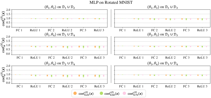
Figure 14: Distribution of $\text{coef}_{\alpha}^{(\ell)}(\boldsymbol{x})$ across the datasets. Here, $\{\boldsymbol{\theta}_{i}\}_{i=1}^{4}$ and $\{\mathcal{D}_{i}\}_{i=1}^{4}$ denotes four finetuned MLPs on the corresponding Rotated MNIST with rotation $\in\{22.5^{\circ},45^{\circ},67.5^{\circ},90^{\circ}\}$ respectively. The results are reported for all layers except classification head of finetuned MLPs, with $\alpha\in\{0.25,0.5,0.75\}$.

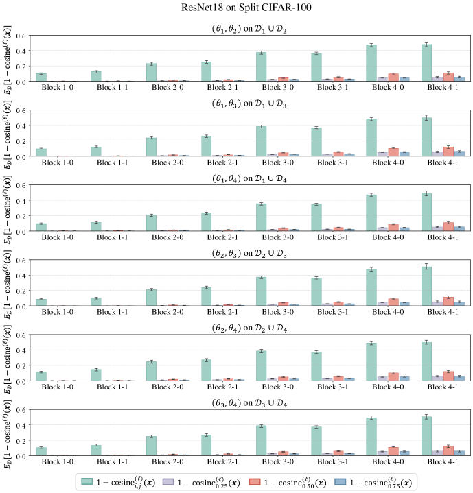
Figure 15: Compare $\mathbb{E}_{\mathcal{D}}[1-{\rm cosine}_{\alpha}^{(\ell)}(\boldsymbol{x})]$ with $\mathbb{E}_{\mathcal{D}}[1-\text{cosine}_{i,j}^{(\ell)}(\boldsymbol{x})]$. Here, $\{\boldsymbol{\theta}_{i}\}_{i=1}^{4}$ and $\{\mathcal{D}_{i}\}_{i=1}^{4}$ denotes four finetuned ResNet-18s and the second to fifth splits in Split CIFAR-100 respectively. The results are reported for all blocks of finetuned ResNet-18 models, with $\alpha\in\{0.25,0.5,0.75\}$.

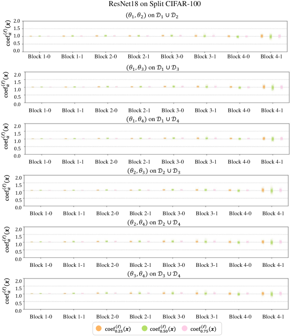
Figure 16: Distribution of $\text{coef}_{\alpha}^{(\ell)}(\boldsymbol{x})$ across the datasets. Here, $\{\boldsymbol{\theta}_{i}\}_{i=1}^{4}$ and $\{\mathcal{D}_{i}\}_{i=1}^{4}$ denotes four finetuned ResNet-18s and the second to fifth splits in Split CIFAR-100 respectively. The results are reported for all blocks of finetuned ResNet-18 models, with $\alpha\in\{0.25,0.5,0.75\}$.

In this section, we provide more experimental results for different task combinations and different layers, which shows the CTL holds in the pretraining-finetuning paradigm. In Figure 13 and LABEL:{fig:LLFC_appendix_mlp_coef}, we include experimental results of $\mathbb{E}_{\mathcal{D}}[1-{\rm cosine}_{\alpha}^{(\ell)}(\boldsymbol{x})]$ and $\text{coef}_{\alpha}^{(\ell)}(\boldsymbol{x})$ for MLPs on Rotated MNIST dataset. In Figure 15 and LABEL:{fig:LLFC_appendix_resnet18_coef}, we include experimental results of $\mathbb{E}_{\mathcal{D}}[1-{\rm cosine}_{\alpha}^{(\ell)}(\boldsymbol{x})]$ and $\text{coef}_{\alpha}^{(\ell)}(\boldsymbol{x})$ for ResNet-18 on Split CIFAR-100 dataset.

B.5 More Verification of Equation 1

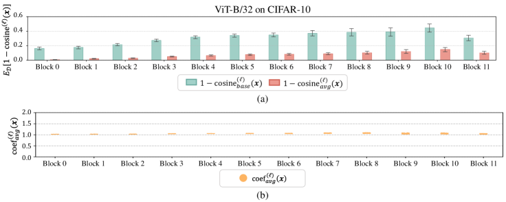
Figure 17: (a) Compare $\mathbb{E}_{\mathcal{D}}[1-{\rm cosine}_{avg}^{(\ell)}(\boldsymbol{x})]$ with $\mathbb{E}_{\mathcal{D}}[1-{\rm cosine}_{base}^{(\ell)}(\boldsymbol{x})]$. (b) Distribution of ${\rm coef}_{avg}^{(\ell)}(\boldsymbol{x})$ on CIFAR-10. The results are reported for all blocks of ViT-B/32 models, that are finetuned on CIFAR-10 with different hyper-parameters.

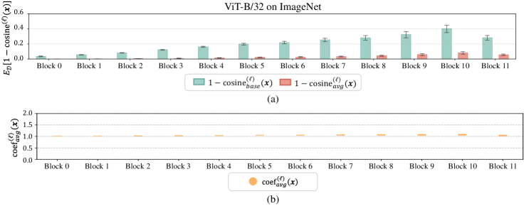
Figure 18: (a) Compare $\mathbb{E}_{\mathcal{D}}[1-{\rm cosine}_{avg}^{(\ell)}(\boldsymbol{x})]$ with $\mathbb{E}_{\mathcal{D}}[1-{\rm cosine}_{base}^{(\ell)}(\boldsymbol{x})]$. (b) Distribution of ${\rm coef}_{avg}^{(\ell)}(\boldsymbol{x})$ on ImageNet. The results are reported for all blocks of ViT-B/32 models, that are finetuned on ImageNet with different hyper-parameters.

In this section, we provide more experimental results for ViT-B/32 to validate Equation 1. In Figure 17, we include the $\mathbb{E}_{\mathcal{D}}[1-{\rm cosine}_{avg}^{(\ell)}(\boldsymbol{x})]$ and ${\rm coef}_{avg}^{(\ell)}(\boldsymbol{x})$ for ViT-B/32 on CIFAR-10. In Figure 18, we include the $\mathbb{E}_{\mathcal{D}}[1-{\rm cosine}_{avg}^{(\ell)}(\boldsymbol{x})]$ and ${\rm coef}_{avg}^{(\ell)}(\boldsymbol{x})$ for ViT-B/32 on ImageNet. Results are reported across all blocks of ViT-B/32.

B.6 More Verification of Equation 2

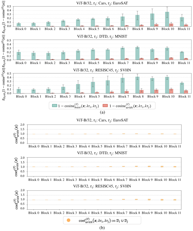
Figure 19: (a) Compare $\mathbb{E}_{\mathcal{D}}[1-{\rm cosine}_{arith}^{(\ell)}(\boldsymbol{x};\lambda\tau_{i},\lambda\tau_{j})]$ with $\mathbb{E}_{\mathcal{D}}[1-{\rm cosine}_{base}^{(\ell)}(\boldsymbol{x};\lambda\tau_{i},\lambda\tau_{j})]$. The bottom and top of the error bar represent the lower and upper quartile of the values across the dataset, respectively. (b) Distribution of ${\rm coef}_{arith}^{(\ell)}(\boldsymbol{x};\lambda\tau_{i},\lambda\tau_{j})$. The results are reported for all blocks of finetuned ViT-B/32 under different settings, with $\lambda=0.4$ and $\alpha=0.5$.

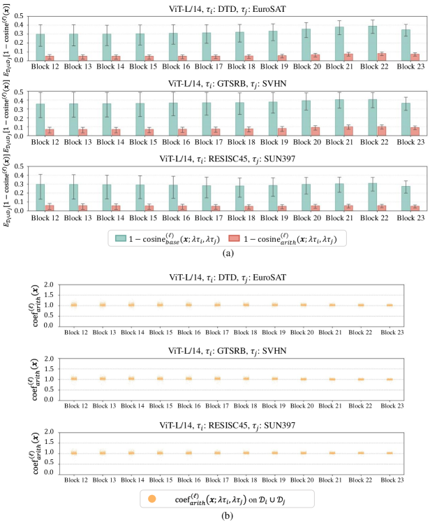
Figure 20: (a) Compare $\mathbb{E}_{\mathcal{D}}[1-{\rm cosine}_{arith}^{(\ell)}(\boldsymbol{x};\lambda\tau_{i},\lambda\tau_{j})]$ with $\mathbb{E}_{\mathcal{D}}[1-{\rm cosine}_{base}^{(\ell)}(\boldsymbol{x};\lambda\tau_{i},\lambda\tau_{j})]$. The bottom and top of the error bar represent the lower and upper quartile of the values across the dataset, respectively. (b) Distribution of ${\rm coef}_{arith}^{(\ell)}(\boldsymbol{x};\lambda\tau_{i},\lambda\tau_{j})$. The results are reported for the last $12$ blocks of finetuned ViT-L/14 under different settings, with $\lambda=0.4$ and $\alpha=0.5$.

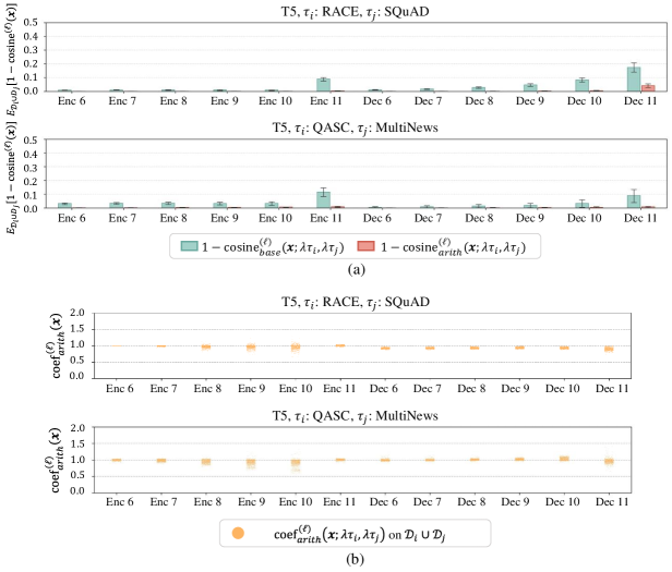
Figure 21: (a) Compare $\mathbb{E}_{\mathcal{D}}[1-{\rm cosine}_{arith}^{(\ell)}(\boldsymbol{x};\lambda\tau_{i},\lambda\tau_{j})]$ with $\mathbb{E}_{\mathcal{D}}[1-{\rm cosine}_{base}^{(\ell)}(\boldsymbol{x};\lambda\tau_{i},\lambda\tau_{j})]$. The bottom and top of the error bar represent the lower and upper quartile of the values across the dataset, respectively. (b) Distribution of ${\rm coef}_{arith}^{(\ell)}(\boldsymbol{x};\lambda\tau_{i},\lambda\tau_{j})$. The results are reported for the last $6$ encoder blocks and the last $6$ decoder blocks of finetuned T5 under different settings, with $\lambda=0.4$ and $\alpha=0.5$.

In this section, we provide more experimental results to validate Equation 2. We provide results for more combinations of task vectors of ViT-B/32, ViT-L/14 and T5 architectures. We report both $\mathbb{E}_{\mathcal{D}}[1-{\rm cosine}_{arith}^{(\ell)}(\boldsymbol{x};\lambda\tau_{i},\lambda\tau_{j})]$ and ${\rm coef}_{arith}^{(\ell)}(\boldsymbol{x};\lambda\tau_{i},\lambda\tau_{j})$. In Figure 19, we provide more results for ViT-B/32 architecture and report all the blocks of ViT-B/32. In Figure 20, we provide more results for ViT-L/14 architecture and report the last $12$ blocks of ViT-L/14. In Figure 21, we provide more results for T5 architecture and report the last $6$ encoder blocks and last $6$ decoder blocks of T5.

B.7 More Verification of Equation 3

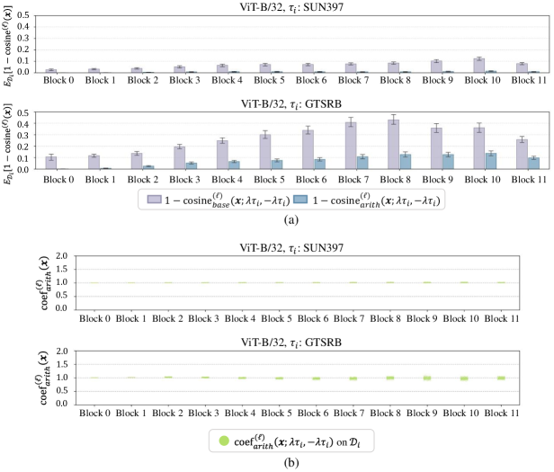
Figure 22: (a) Compare $\mathbb{E}_{\mathcal{D}}[1-{\rm cosine}_{arith}^{(\ell)}(\boldsymbol{x};\lambda\tau_{i},-\lambda\tau_{i})]$ with $\mathbb{E}_{\mathcal{D}}[1-{\rm cosine}_{base}^{(\ell)}(\boldsymbol{x};\lambda\tau_{i},-\lambda\tau_{i})]$. The bottom and top of the error bar represent the lower and upper quartile of the values across the dataset, respectively. (b) Distribution of ${\rm coef}_{arith}^{(\ell)}(\boldsymbol{x};\lambda\tau_{i},-\lambda\tau_{i})$. The results are reported for all blocks of finetuned ViT-B/32 under different settings, with $\lambda=0.4$ and $\alpha=0.5$.

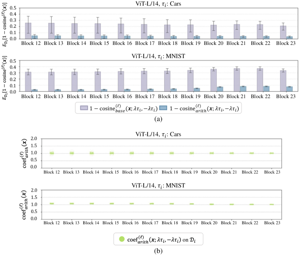
Figure 23: (a) Compare $\mathbb{E}_{\mathcal{D}}[1-{\rm cosine}_{arith}^{(\ell)}(\boldsymbol{x};\lambda\tau_{i},-\lambda\tau_{i})]$ with $\mathbb{E}_{\mathcal{D}}[1-{\rm cosine}_{base}^{(\ell)}(\boldsymbol{x};\lambda\tau_{i},-\lambda\tau_{i})]$. The bottom and top of the error bar represent the lower and upper quartile of the values across the dataset, respectively. (b) Distribution of ${\rm coef}_{arith}^{(\ell)}(\boldsymbol{x};\lambda\tau_{i},-\lambda\tau_{i})$. The results are reported for the last $12$ blocks of finetuned ViT-L/14 under different settings, with $\lambda=0.4$ and $\alpha=0.5$.

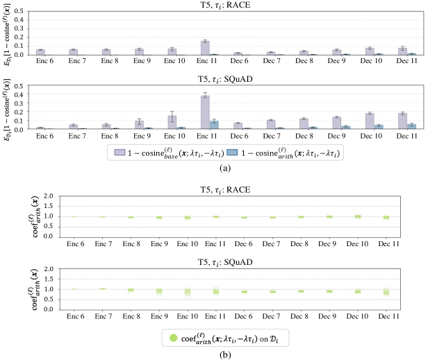
Figure 24: (a) Compare $\mathbb{E}_{\mathcal{D}}[1-{\rm cosine}_{arith}^{(\ell)}(\boldsymbol{x};\lambda\tau_{i},-\lambda\tau_{i})]$ with $\mathbb{E}_{\mathcal{D}}[1-{\rm cosine}_{base}^{(\ell)}(\boldsymbol{x};\lambda\tau_{i},-\lambda\tau_{i})]$. The bottom and top of the error bar represent the lower and upper quartile of the values across the dataset, respectively. (b) Distribution of ${\rm coef}_{arith}^{(\ell)}(\boldsymbol{x};\lambda\tau_{i},-\lambda\tau_{i})$. The results are reported for the last $6$ encoder blocks and the last $6$ decoder blocks of finetuned T5 under different settings, with $\lambda=0.4$ and $\alpha=0.5$.

In this section, we provide more experimental results to validate Equation 3. We provide results for more task vectors of ViT-B/32, ViT-L/14 and T5 architectures. We report both $\mathbb{E}_{\mathcal{D}}[1-{\rm cosine}_{arith}^{(\ell)}(\boldsymbol{x};\lambda\tau_{i},-\lambda\tau_{i})]$ and ${\rm coef}_{arith}^{(\ell)}(\boldsymbol{x};\lambda\tau_{i},-\lambda\tau_{i})$. In Figure 22, we provide more results for ViT-B/32 architecture and report all the blocks of ViT-B/32. In Figure 23, we provide more results for ViT-L/14 architecture and report the last 12 blocks of ViT-L/14. In Figure 24, we provide more results for T5 architecture and report the last 6 encoder blocks and last 6 decoder blocks of T5.

References

- Adilova et al. [2023] Linara Adilova, Asja Fischer, and Martin Jaggi. Layerwise linear mode connectivity. arXiv preprint arXiv:2307.06966, 2023.
- Ainsworth et al. [2023] Samuel Ainsworth, Jonathan Hayase, and Siddhartha Srinivasa. Git re-basin: Merging models modulo permutation symmetries. In The Eleventh International Conference on Learning Representations, 2023. URL https://openreview.net/forum?id=CQsmMYmlP5T.
- Bansal et al. [2021] Yamini Bansal, Preetum Nakkiran, and Boaz Barak. Revisiting model stitching to compare neural representations. In A. Beygelzimer, Y. Dauphin, P. Liang, and J. Wortman Vaughan, editors, Advances in Neural Information Processing Systems, 2021. URL https://openreview.net/forum?id=ak06J5jNR4.
- Cheng et al. [2017] Gong Cheng, Junwei Han, and Xiaoqiang Lu. Remote sensing image scene classification: Benchmark and state of the art. Proceedings of the IEEE, 105(10):1865–1883, 2017.
- Cimpoi et al. [2014] Mircea Cimpoi, Subhransu Maji, Iasonas Kokkinos, Sammy Mohamed, and Andrea Vedaldi. Describing textures in the wild. In Proceedings of the IEEE conference on computer vision and pattern recognition, pages 3606–3613, 2014.
- Dosovitskiy et al. [2020] Alexey Dosovitskiy, Lucas Beyer, Alexander Kolesnikov, Dirk Weissenborn, Xiaohua Zhai, Thomas Unterthiner, Mostafa Dehghani, Matthias Minderer, Georg Heigold, Sylvain Gelly, et al. An image is worth 16x16 words: Transformers for image recognition at scale. arXiv preprint arXiv:2010.11929, 2020.
- Draxler et al. [2018] Felix Draxler, Kambis Veschgini, Manfred Salmhofer, and Fred Hamprecht. Essentially no barriers in neural network energy landscape. In International conference on machine learning, pages 1309–1318. PMLR, 2018.
- Elhage et al. [2021] Nelson Elhage, Neel Nanda, Catherine Olsson, Tom Henighan, Nicholas Joseph, Ben Mann, Amanda Askell, Yuntao Bai, Anna Chen, Tom Conerly, Nova DasSarma, Dawn Drain, Deep Ganguli, Zac Hatfield-Dodds, Danny Hernandez, Andy Jones, Jackson Kernion, Liane Lovitt, Kamal Ndousse, Dario Amodei, Tom Brown, Jack Clark, Jared Kaplan, Sam McCandlish, and Chris Olah. A mathematical framework for transformer circuits. Transformer Circuits Thread, 2021. https://transformer-circuits.pub/2021/framework/index.html.
- Entezari et al. [2022] Rahim Entezari, Hanie Sedghi, Olga Saukh, and Behnam Neyshabur. The role of permutation invariance in linear mode connectivity of neural networks. In International Conference on Learning Representations, 2022. URL https://openreview.net/forum?id=dNigytemkL.
- Fabbri et al. [2019] Alexander R Fabbri, Irene Li, Tianwei She, Suyi Li, and Dragomir R Radev. Multi-news: A large-scale multi-document summarization dataset and abstractive hierarchical model. arXiv preprint arXiv:1906.01749, 2019.
- Ferbach et al. [2023] Damien Ferbach, Baptiste Goujaud, Gauthier Gidel, and Aymeric Dieuleveut. Proving linear mode connectivity of neural networks via optimal transport. arXiv preprint arXiv:2310.19103, 2023.
- Fort et al. [2020] Stanislav Fort, Gintare Karolina Dziugaite, Mansheej Paul, Sepideh Kharaghani, Daniel M Roy, and Surya Ganguli. Deep learning versus kernel learning: an empirical study of loss landscape geometry and the time evolution of the neural tangent kernel. Advances in Neural Information Processing Systems, 33:5850–5861, 2020.
- Frankle et al. [2020a] Jonathan Frankle, Gintare Karolina Dziugaite, Daniel Roy, and Michael Carbin. Linear mode connectivity and the lottery ticket hypothesis. In International Conference on Machine Learning, pages 3259–3269. PMLR, 2020a.
- Frankle et al. [2020b] Jonathan Frankle, David J. Schwab, and Ari S. Morcos. The early phase of neural network training. In International Conference on Learning Representations, 2020b. URL https://openreview.net/forum?id=Hkl1iRNFwS.
- Freeman and Bruna [2017] C. Daniel Freeman and Joan Bruna. Topology and geometry of half-rectified network optimization. In International Conference on Learning Representations, 2017. URL https://openreview.net/forum?id=Bk0FWVcgx.
- Garipov et al. [2018] Timur Garipov, Pavel Izmailov, Dmitrii Podoprikhin, Dmitry P Vetrov, and Andrew G Wilson. Loss surfaces, mode connectivity, and fast ensembling of dnns. Advances in neural information processing systems, 31, 2018.
- He et al. [2016] Kaiming He, Xiangyu Zhang, Shaoqing Ren, and Jian Sun. Deep residual learning for image recognition. In 2016 IEEE Conference on Computer Vision and Pattern Recognition (CVPR), pages 770–778, 2016. doi: 10.1109/CVPR.2016.90.
- Helber et al. [2019] Patrick Helber, Benjamin Bischke, Andreas Dengel, and Damian Borth. Eurosat: A novel dataset and deep learning benchmark for land use and land cover classification. IEEE Journal of Selected Topics in Applied Earth Observations and Remote Sensing, 12(7):2217–2226, 2019.
- Ilharco et al. [2022] Gabriel Ilharco, Mitchell Wortsman, Samir Yitzhak Gadre, Shuran Song, Hannaneh Hajishirzi, Simon Kornblith, Ali Farhadi, and Ludwig Schmidt. Patching open-vocabulary models by interpolating weights. In Alice H. Oh, Alekh Agarwal, Danielle Belgrave, and Kyunghyun Cho, editors, Advances in Neural Information Processing Systems, 2022. URL https://openreview.net/forum?id=CZZFRxbOLC.
- Ilharco et al. [2023] Gabriel Ilharco, Marco Tulio Ribeiro, Mitchell Wortsman, Ludwig Schmidt, Hannaneh Hajishirzi, and Ali Farhadi. Editing models with task arithmetic. In The Eleventh International Conference on Learning Representations, 2023. URL https://openreview.net/forum?id=6t0Kwf8-jrj.
- Izmailov et al. [2018] Pavel Izmailov, Dmitrii Podoprikhin, Timur Garipov, Dmitry P. Vetrov, and Andrew Gordon Wilson. Averaging weights leads to wider optima and better generalization. In Amir Globerson and Ricardo Silva, editors, Proceedings of the Thirty-Fourth Conference on Uncertainty in Artificial Intelligence, UAI 2018, Monterey, California, USA, August 6-10, 2018, pages 876–885. AUAI Press, 2018. URL http://auai.org/uai2018/proceedings/papers/313.pdf.
- Jin et al. [2023] Xisen Jin, Xiang Ren, Daniel Preotiuc-Pietro, and Pengxiang Cheng. Dataless knowledge fusion by merging weights of language models. In The Eleventh International Conference on Learning Representations, 2023. URL https://openreview.net/forum?id=FCnohuR6AnM.
- Juneja et al. [2023] Jeevesh Juneja, Rachit Bansal, Kyunghyun Cho, João Sedoc, and Naomi Saphra. Linear connectivity reveals generalization strategies. In The Eleventh International Conference on Learning Representations, 2023. URL https://openreview.net/forum?id=hY6M0JHl3uL.
- Khot et al. [2020] Tushar Khot, Peter Clark, Michal Guerquin, Peter Jansen, and Ashish Sabharwal. Qasc: A dataset for question answering via sentence composition. In Proceedings of the AAAI Conference on Artificial Intelligence, volume 34, pages 8082–8090, 2020.
- Krause et al. [2013] Jonathan Krause, Michael Stark, Jia Deng, and Li Fei-Fei. 3d object representations for fine-grained categorization. 2013 IEEE International Conference on Computer Vision Workshops, pages 554–561, 2013. URL https://api.semanticscholar.org/CorpusID:14342571.
- Kuditipudi et al. [2019] Rohith Kuditipudi, Xiang Wang, Holden Lee, Yi Zhang, Zhiyuan Li, Wei Hu, Rong Ge, and Sanjeev Arora. Explaining landscape connectivity of low-cost solutions for multilayer nets. Advances in neural information processing systems, 32, 2019.
- Lai et al. [2017] Guokun Lai, Qizhe Xie, Hanxiao Liu, Yiming Yang, and Eduard Hovy. Race: Large-scale reading comprehension dataset from examinations. arXiv preprint arXiv:1704.04683, 2017.
- LeCun and Cortes [2005] Yann LeCun and Corinna Cortes. The mnist database of handwritten digits. 2005. URL https://api.semanticscholar.org/CorpusID:60282629.
- Lenc and Vedaldi [2015] Karel Lenc and Andrea Vedaldi. Understanding image representations by measuring their equivariance and equivalence. In Proceedings of the IEEE conference on computer vision and pattern recognition, pages 991–999, 2015.
- Li et al. [2022] Margaret Li, Suchin Gururangan, Tim Dettmers, Mike Lewis, Tim Althoff, Noah A. Smith, and Luke Zettlemoyer. Branch-train-merge: Embarrassingly parallel training of expert language models. In First Workshop on Interpolation Regularizers and Beyond at NeurIPS 2022, 2022. URL https://openreview.net/forum?id=SQgVgE2Sq4.
- Liang et al. [2018] Shiyu Liang, Ruoyu Sun, Yixuan Li, and Rayadurgam Srikant. Understanding the loss surface of neural networks for binary classification. In International Conference on Machine Learning, pages 2835–2843. PMLR, 2018.
- Lin et al. [2019] Bill Yuchen Lin, Wangchunshu Zhou, Ming Shen, Pei Zhou, Chandra Bhagavatula, Yejin Choi, and Xiang Ren. Commongen: A constrained text generation challenge for generative commonsense reasoning. arXiv preprint arXiv:1911.03705, 2019.
- Liu et al. [2022] Chang Liu, Chenfei Lou, Runzhong Wang, Alan Yuhan Xi, Li Shen, and Junchi Yan. Deep neural network fusion via graph matching with applications to model ensemble and federated learning. In Kamalika Chaudhuri, Stefanie Jegelka, Le Song, Csaba Szepesvari, Gang Niu, and Sivan Sabato, editors, Proceedings of the 39th International Conference on Machine Learning, volume 162 of Proceedings of Machine Learning Research, pages 13857–13869. PMLR, 17–23 Jul 2022. URL https://proceedings.mlr.press/v162/liu22k.html.
- Maas et al. [2011] Andrew Maas, Raymond E Daly, Peter T Pham, Dan Huang, Andrew Y Ng, and Christopher Potts. Learning word vectors for sentiment analysis. In Proceedings of the 49th annual meeting of the association for computational linguistics: Human language technologies, pages 142–150, 2011.
- Matena and Raffel [2022] Michael S Matena and Colin Raffel. Merging models with fisher-weighted averaging. In Alice H. Oh, Alekh Agarwal, Danielle Belgrave, and Kyunghyun Cho, editors, Advances in Neural Information Processing Systems, 2022. URL https://openreview.net/forum?id=LSKlp_aceOC.
- McCloskey and Cohen [1989] Michael McCloskey and Neal J Cohen. Catastrophic interference in connectionist networks: The sequential learning problem. In Psychology of learning and motivation, volume 24, pages 109–165. Elsevier, 1989.
- Mirzadeh et al. [2021] Seyed Iman Mirzadeh, Mehrdad Farajtabar, Dilan Gorur, Razvan Pascanu, and Hassan Ghasemzadeh. Linear mode connectivity in multitask and continual learning. In International Conference on Learning Representations, 2021. URL https://openreview.net/forum?id=Fmg_fQYUejf.
- Nagarajan and Kolter [2019] Vaishnavh Nagarajan and J Zico Kolter. Uniform convergence may be unable to explain generalization in deep learning. Advances in Neural Information Processing Systems, 32, 2019.
- Netzer et al. [2011] Yuval Netzer, Tao Wang, Adam Coates, Alessandro Bissacco, Bo Wu, and Andrew Y Ng. Reading digits in natural images with unsupervised feature learning. 2011.
- Nguyen [2019] Quynh Nguyen. On connected sublevel sets in deep learning. In International conference on machine learning, pages 4790–4799. PMLR, 2019.
- Nguyen et al. [2019] Quynh Nguyen, Mahesh Chandra Mukkamala, and Matthias Hein. On the loss landscape of a class of deep neural networks with no bad local valleys. In International Conference on Learning Representations, 2019. URL https://openreview.net/forum?id=HJgXsjA5tQ.
- Ni et al. [2021] Jianmo Ni, Gustavo Hernández Ábrego, Noah Constant, Ji Ma, Keith B Hall, Daniel Cer, and Yinfei Yang. Sentence-t5: Scalable sentence encoders from pre-trained text-to-text models. arXiv preprint arXiv:2108.08877, 2021.
- Olsson et al. [2022] Catherine Olsson, Nelson Elhage, Neel Nanda, Nicholas Joseph, Nova DasSarma, Tom Henighan, Ben Mann, Amanda Askell, Yuntao Bai, Anna Chen, Tom Conerly, Dawn Drain, Deep Ganguli, Zac Hatfield-Dodds, Danny Hernandez, Scott Johnston, Andy Jones, Jackson Kernion, Liane Lovitt, Kamal Ndousse, Dario Amodei, Tom Brown, Jack Clark, Jared Kaplan, Sam McCandlish, and Chris Olah. In-context learning and induction heads. Transformer Circuits Thread, 2022. https://transformer-circuits.pub/2022/in-context-learning-and-induction-heads/index.html.
- Ortiz-Jimenez et al. [2023] Guillermo Ortiz-Jimenez, Alessandro Favero, and Pascal Frossard. Task arithmetic in the tangent space: Improved editing of pre-trained models. In Thirty-seventh Conference on Neural Information Processing Systems, 2023. URL https://openreview.net/forum?id=0A9f2jZDGW.
- Ouyang et al. [2022] Long Ouyang, Jeffrey Wu, Xu Jiang, Diogo Almeida, Carroll Wainwright, Pamela Mishkin, Chong Zhang, Sandhini Agarwal, Katarina Slama, Alex Gray, John Schulman, Jacob Hilton, Fraser Kelton, Luke Miller, Maddie Simens, Amanda Askell, Peter Welinder, Paul Christiano, Jan Leike, and Ryan Lowe. Training language models to follow instructions with human feedback. In Alice H. Oh, Alekh Agarwal, Danielle Belgrave, and Kyunghyun Cho, editors, Advances in Neural Information Processing Systems, 2022. URL https://openreview.net/forum?id=TG8KACxEON.
- Qin et al. [2022] Yujia Qin, Cheng Qian, Jing Yi, Weize Chen, Yankai Lin, Xu Han, Zhiyuan Liu, Maosong Sun, and Jie Zhou. Exploring mode connectivity for pre-trained language models. In Yoav Goldberg, Zornitsa Kozareva, and Yue Zhang, editors, Proceedings of the 2022 Conference on Empirical Methods in Natural Language Processing, pages 6726–6746, Abu Dhabi, United Arab Emirates, December 2022. Association for Computational Linguistics. doi: 10.18653/v1/2022.emnlp-main.451. URL https://aclanthology.org/2022.emnlp-main.451.
- Raffel et al. [2020] Colin Raffel, Noam Shazeer, Adam Roberts, Katherine Lee, Sharan Narang, Michael Matena, Yanqi Zhou, Wei Li, and Peter J Liu. Exploring the limits of transfer learning with a unified text-to-text transformer. The Journal of Machine Learning Research, 21(1):5485–5551, 2020.
- Rajpurkar et al. [2016] Pranav Rajpurkar, Jian Zhang, Konstantin Lopyrev, and Percy Liang. Squad: 100,000+ questions for machine comprehension of text. arXiv preprint arXiv:1606.05250, 2016.
- Rame et al. [2022] Alexandre Rame, Matthieu Kirchmeyer, Thibaud Rahier, Alain Rakotomamonjy, patrick gallinari, and Matthieu Cord. Diverse weight averaging for out-of-distribution generalization. In Alice H. Oh, Alekh Agarwal, Danielle Belgrave, and Kyunghyun Cho, editors, Advances in Neural Information Processing Systems, 2022. URL https://openreview.net/forum?id=tq_J_MqB3UB.
- Rame et al. [2023] Alexandre Rame, Kartik Ahuja, Jianyu Zhang, Matthieu Cord, Leon Bottou, and David Lopez-Paz. Model ratatouille: Recycling diverse models for out-of-distribution generalization. In Andreas Krause, Emma Brunskill, Kyunghyun Cho, Barbara Engelhardt, Sivan Sabato, and Jonathan Scarlett, editors, Proceedings of the 40th International Conference on Machine Learning, volume 202 of Proceedings of Machine Learning Research, pages 28656–28679. PMLR, 23–29 Jul 2023. URL https://proceedings.mlr.press/v202/rame23a.html.
- Singh and Jaggi [2020] Sidak Pal Singh and Martin Jaggi. Model fusion via optimal transport. Advances in Neural Information Processing Systems, 33:22045–22055, 2020.
- Stallkamp et al. [2011] Johannes Stallkamp, Marc Schlipsing, Jan Salmen, and Christian Igel. The german traffic sign recognition benchmark: a multi-class classification competition. In The 2011 international joint conference on neural networks, pages 1453–1460. IEEE, 2011.
- Stoica et al. [2023] George Stoica, Daniel Bolya, Jakob Bjorner, Taylor Hearn, and Judy Hoffman. Zipit! merging models from different tasks without training, 2023.
- Venturi et al. [2019] Luca Venturi, Afonso S. Bandeira, and Joan Bruna. Spurious valleys in one-hidden-layer neural network optimization landscapes. J. Mach. Learn. Res., 20:133:1–133:34, 2019. URL http://jmlr.org/papers/v20/18-674.html.
- Weidinger et al. [2021] Laura Weidinger, John Mellor, Maribeth Rauh, Conor Griffin, Jonathan Uesato, Po-Sen Huang, Myra Cheng, Mia Glaese, Borja Balle, Atoosa Kasirzadeh, Zac Kenton, Sasha Brown, Will Hawkins, Tom Stepleton, Courtney Biles, Abeba Birhane, Julia Haas, Laura Rimell, Lisa Anne Hendricks, William Isaac, Sean Legassick, Geoffrey Irving, and Iason Gabriel. Ethical and social risks of harm from language models, 2021.
- Wortsman et al. [2022a] Mitchell Wortsman, Gabriel Ilharco, Samir Ya Gadre, Rebecca Roelofs, Raphael Gontijo-Lopes, Ari S Morcos, Hongseok Namkoong, Ali Farhadi, Yair Carmon, Simon Kornblith, et al. Model soups: averaging weights of multiple fine-tuned models improves accuracy without increasing inference time. In International Conference on Machine Learning, pages 23965–23998. PMLR, 2022a.
- Wortsman et al. [2022b] Mitchell Wortsman, Gabriel Ilharco, Jong Wook Kim, Mike Li, Simon Kornblith, Rebecca Roelofs, Raphael Gontijo Lopes, Hannaneh Hajishirzi, Ali Farhadi, Hongseok Namkoong, and Ludwig Schmidt. Robust fine-tuning of zero-shot models. In Proceedings of the IEEE/CVF Conference on Computer Vision and Pattern Recognition (CVPR), pages 7959–7971, June 2022b.
- Xiao et al. [2016] Jianxiong Xiao, Krista A Ehinger, James Hays, Antonio Torralba, and Aude Oliva. Sun database: Exploring a large collection of scene categories. International Journal of Computer Vision, 119:3–22, 2016.
- Yadav et al. [2023] Prateek Yadav, Derek Tam, Leshem Choshen, Colin Raffel, and Mohit Bansal. TIES-merging: Resolving interference when merging models. In Thirty-seventh Conference on Neural Information Processing Systems, 2023. URL https://openreview.net/forum?id=xtaX3WyCj1.
- Yu et al. [2023] Le Yu, Bowen Yu, Haiyang Yu, Fei Huang, and Yongbin Li. Language models are super mario: Absorbing abilities from homologous models as a free lunch, 2023.
- Yunis et al. [2022] David Yunis, Kumar Kshitij Patel, Pedro Henrique Pamplona Savarese, Gal Vardi, Jonathan Frankle, Matthew Walter, Karen Livescu, and Michael Maire. On convexity and linear mode connectivity in neural networks. In OPT 2022: Optimization for Machine Learning (NeurIPS 2022 Workshop), 2022. URL https://openreview.net/forum?id=TZQ3PKL3fPr.
- Zhao et al. [2023] Bo Zhao, Nima Dehmamy, Robin Walters, and Rose Yu. Understanding mode connectivity via parameter space symmetry. In UniReps: the First Workshop on Unifying Representations in Neural Models, 2023. URL https://openreview.net/forum?id=aP2a5i1iUf.
- Zhou et al. [2023] Zhanpeng Zhou, Yongyi Yang, Xiaojiang Yang, Junchi Yan, and Wei Hu. Going beyond linear mode connectivity: The layerwise linear feature connectivity. In Thirty-seventh Conference on Neural Information Processing Systems, 2023. URL https://openreview.net/forum?id=vORUHrVEnH.