Discretization form of the continuity condition at the polar axis, with application to the gyrokinetic simulation in a magnetic fusion torus

Abstract

A new computational method to solve the hyperbolic (Vlasov) equation coupled to the elliptic (Poisson-like) equation at the polar axis is proposed. It is shown that the value of a scalar function at the polar axis can be predicted by its neighbouring values based on the continuity condition. This continuity condition systematically solves the pole problems including the singular factor $1/r$ in the hyperbolic equation and the inner boundary in the elliptic equation. The proposed method is applied to the global gyrokinetic simulation of the tokamak plasma with the magnetic axis included.

1 Introduction

The difficulties in numerically solving partial differential equations (PDEs) at the polar axis in polar coordinates have attracted significant interest for many years. These difficulties, which are noted as pole problems in this paper, are related to (i) terms containing the geometrical singular factor $1/r$ [1], with $r$ the radial position, (ii) inner boundary conditions needed to been specified at $r=0$ [2, 3], even if physically there is no boundary at the polar axis, (iii) the severe numerical error of low-order finite-difference schemes, such as the second-order central difference.

In the framework of the finite-difference method (FDM) or the pseudo-spectrum method (PSM), several computational methods have been proposed to solve the pole problems. The main idea of the PSM [4] to solve problem (i) is to use polynomial expansions in the radial direction that satisfy the regularity condition in the Cartesian coordinates. The series in radius, such as the Bessel functions or one-sided Jacobi polynomials [5, 6], can analytically remove singular terms, and thus no additional inner boundary conditions are necessary [4]. If the radial series do not completely satisfy the continuity condition, ”pole conditions” [3] are preferred to replace the PDEs at the polar axis. In the PSM, the relative high numerical error near the polar axis is possible connected with the problem (ii), which can be understood as the behaviour of the global high order polynomial interpolation near the boundary [7]. One method to solve this problem is to refine the radial girds near the polar axis [3]. Another method is to use the computational domain mapping $\boldsymbol{M}:(0,1)\times(-\pi,\pi)\to(-1,1)\times(\pi/2,\pi/2)$ on a unit disk [7], where the polar axis is not treated as the inner boundary, and thus radial grid points near the polar axis will not need to be refined.

Although the FDM is less accurate than the PSM, the treatment of pole problems in the FDM is of significant interest, due to its conveniences in handling complex geometrical configurations [1] and nonlinear computation. For problem (i), series expansions derived from the regularity condition are used to analytically remove singular factors at the polar axis [1]. Moreover, singular terms can also be avoided by shifting the grid points in the radial direction [8] so that there is no grid point situated at the polar axis. However, the shifted radial grid points may lead to the more severe numerical error of the computation of singular terms [1] at the first point off the axis. For problem (ii), the computational domain mapping $\boldsymbol{M}$ is used to avoid the inner boundary in the FDM [1, 8], which avoids the use of the one-sided finite-difference [2]. For problem (iii), highly accurate finite-difference schemes, such as Pade schemes [9], are used to improve the accuracy of the FDM [1]. In Pade schemes, a derivative is evaluated by the values on all grid points. The numerical error of the FDM in a high wavenumber test is considerably lowered by these schemes [9].

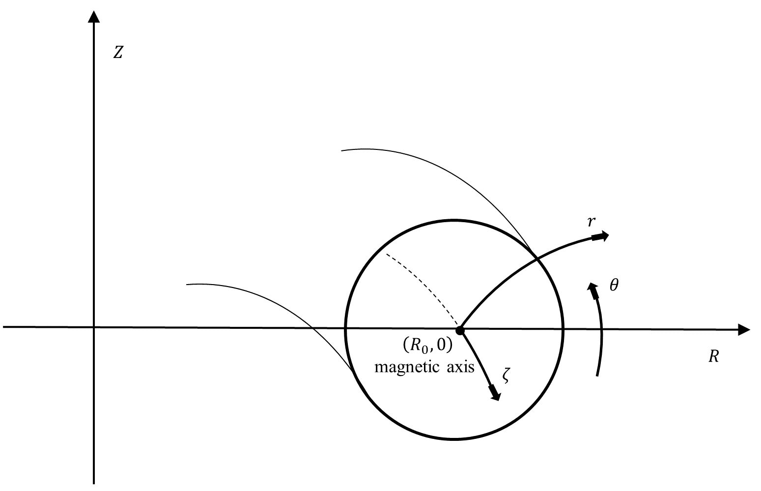
Figure 1: Magnetic flux coordinates and cylindrical coordinates.

The pole problems are of significant interest in the global gyrokinetic (GK) simulation [10] in the tokamak fusion plasma, since the magnetic axis of the fusion torus is essentially a polar axis. To simulate the ion temperature gradient (ITG) driven mode in a fusion torus with adiabatic electrons, one has to solve the GK Vlasov-Poisson (VP) system. However, the GK VP system is very computationally expensive, which simulates the time evolution of the distribution function $F(\boldsymbol{Z};t)$ and the perturbed electrostatic potential $\delta\phi(\boldsymbol{X};t)$, where $\boldsymbol{Z}=(\boldsymbol{X},v_{\parallel},\mu)$ are the phase space coordinates, $\boldsymbol{X}$ is the position of the gyrocenter, $v_{\parallel}$ is the the parallel velocity and $\mu$ is the magnetic moment with $\mathrm{d}\mu/\mathrm{d}t=0$. For higher computational efficiency, the system is usually solved in magnetic flux coordinates $\boldsymbol{X}=(r,\theta,\zeta)$, with $r(\psi_{T})\propto\sqrt{\psi_{T}}$ the generalized minor radius, $\psi_{T}$ the toroidal magnetic flux, $\theta$ the poloidal angle and $\zeta$ the toroidal angle. The magnetic flux coordinates discussed are graphically shown in Fig. 1. In these coordinates, the GK Vlasov equation [11] is given by

$$\frac{\partial F}{\partial t}+\dot{r}\frac{\partial F}{\partial r}+\dot{\theta}\frac{\partial F}{\partial\theta}+\dot{\zeta}\frac{\partial F}{\partial\zeta}+\dot{v}_{\parallel}\frac{\partial F}{\partial v_{\parallel}}=0,$$ (1)

which is a hyperbolic equation. The GK quasi-neutrality equation [12] is given by

$$-c_{1}\delta\phi+\int{\mathrm{d}^{3}v\left(\frac{c_{1}}{n_{0}}F\right)\left<\left<\delta\phi\right>\right>_{ga}}-c_{2}(\delta\phi-\left<\delta\phi\right>_{FA})=-e_{i}\rho_{i,gy},$$ (2)

with $c_{1}=\frac{e_{i}^{2}n_{0}}{T_{i}}$, $c_{2}=\frac{e^{2}n_{0}}{T_{e}}$, $\left<\cdot\right>_{FA}$ the magnetic surface averaged operator and $\left<\cdot\right>_{ga}$ the gyro-average operator. Here $n_{0}$ is both the equilibrium ion density and the equilibrium electron density, $m_{i}$ is the ion mass. $T_{i}$ and $e_{i}$ are the ion temperature and charge, respectively; $T_{e}$ and $e$ are the electron temperature and charge, respectively. In the long-wavelength approximation, the GK quasi-neutrality equation becomes the Poisson-like (elliptic) equation [12]

$$\nabla\cdot\left(c_{0}\nabla_{\perp}\delta\phi\right)-c_{1}(\delta\phi-\left<\delta\phi\right>_{FA})=-e_{i}\rho_{i,gy},$$ (3)

with $c_{0}=\frac{n_{0}m_{i}}{B^{2}_{0}}$ and $B_{0}$ the magnetic field at the magnetic axis. When approaching the magnetic axis, $r\to 0$, and $r$ can be understood as the usual minor radius. On a minor cross section, the transformation from magnetic flux coordinates $(r,\theta)$ to cylindrical coordinates $(R,Z)$ near the magnetic axis is given by

$$R-R_{0}=x=r\cos{\theta},$$ (4)

$$Z=y=r\sin{\theta},$$

where $(R-R_{0},Z)$ are essentially the Cartesian coordinates $(x,y)$, and $(r,\theta)$ are essentially the polar coordinates. So the difficulties in the GK simulation at the magnetic axis are essentially the pole problems at the polar axis. When Eq. (3) is numerically solved with $r\to 0$, $\dot{\theta}\to\infty$ is a singular term. This is the problem (i) in the Vlasov (hyperbolic) equation. The inner boundary at the magnetic axis in Eq. (3) is the problem (ii) in the Poisson (elliptic) equation. To include the magnetic axis in the GK simulation, we are forced to solve these problems.

In previous GK simulations, the magnetic axis is usually excluded from the simulation domain in global GK simulations [13, 14, 15]. Recently, several GK codes, such as ORB5 [16], GT5D [17] and GKNET [18], are updated to include the magnetic axis. To avoid the problem (i) in Vlasov equation, cylindrical coordinates are used to avoid the singular terms in these codes [16, 17, 18]. However, abandoning the use of magnetic flux coordinates leads to a lower computational efficiency [16]. Moreover, the Poisson equation is still solved in magnetic flux coordinates in these codes [16, 17, 18]. For the problem (ii), one of the methods is to use a numerical inner boundary condition. Different kinds of inner boundary conditions at the magnetic axis are applied in GK codes. A regular condition $\delta\phi(r=0,\theta,\zeta)=\delta\phi(r=0,\theta=0,\zeta)$ is used in ORB5 [16]; a zero boundary condition at both inner and outer boundaries is used in GTC [19]; a natural boundary condition is used in GT5D [17] at the magnetic axis.

In this paper, a new computational method to solve pole problems is proposed. It is found that the value of a scalar function at the polar axis is predicted by its neighbouring values based on the continuity condition. The problem (i) and problem (ii) are systematically solved by this continuity condition. The proposed method is applied to the global GK simulation of a tokamak fusion plasma, with the magnetic axis included.

The remaining part of this paper is organized as follows. In Section 2, the discretization form of the continuity condition at the polar axis is presented. In Section 3, the application of the proposed method in GK simulation for a tokamak torus is presented. In Section 4, numerical results near the magnetic axis are presented. Finally, the conclusion is presented in Section 5

2 Discretization form of the continuity condition at the polar axis

In this section, the continuity condition at the origin in the Cartesian coordinates and in the polar coordinates is discussed, and its discretization form at the polar axis is presented.

2.1 Continuity condition at the origin in the Cartesian coordinates and in the polar coordinates

The functions to be solved in the hyperbolic equation and the elliptic equation discussed here are physically observable scalars. These equations in mathematical physics can be written in any coordinates. To proceed our discussion, we introduce a fundamental assumption.

Any physical observable scalars $g(\boldsymbol{P})$ are $\mathcal{C}^{\infty}$ in the Euclidean space, with $\boldsymbol{P}$ the space point.

This fundamental assumption shall be referred to as the ”continuity condition”.

Following the fundamental assumption, one finds that in the Cartesian coordinates, the function $g(x,y)$, which is of interest, is $\mathcal{C}^{\infty}$ at the origin. So it can be Taylor expanded, to any desired accuracy, around the origin

$$g(x,y)=\sum_{j=0}^{\infty}\sum_{k=0}^{\infty}\frac{1}{(j+k)!}\binom{j+k}{j}a_{j,k}x^{j}y^{k},$$ (5)

with $a_{j,k}=\frac{\partial^{j+k}g}{\partial^{j}x\partial^{k}y}$ and $\binom{j+k}{j}=\frac{(j+k)!}{j!k!}$.

In different coordinates, the value of a scalar quantity at the same space point should be invariant. Transforming from the Cartesian to the polar coordinates (by using Eq. (4)), one finds that Eq. (5) can be written as

$$\hat{g}(r,\theta)=\sum_{m=-\infty}^{\infty}\left(\sum_{l=0}^{\infty}A_{ml}r^{2l}\right)\left(r^{\lvert m\rvert}e^{im\theta}\right),$$ (6)

where we have regrouped terms with the same poloidal Fourier number $m$ together. The expression of the coefficient $A_{ml}$ in terms of $a_{j,k}$ is not important in the following.

The series expansion shown in Eq. (6) has been obtained in the previous literature [20, 21]. Lewis [20] derived Eq. (6) from the symmetry constraint in polar coordinates and the regularity constraint in Cartesian coordinates. Eisen et al. [21] proved that Eq. (6) could be derived from the regularity condition in the Cartesian coordinates.

We point that Eq. (5) is the representation of the fundamental assumption of continuity condition in Cartesian coordinates, while Eq. (6) is its representation in the polar coordinates.

Eq. (6) can be written as $\hat{g}(r,\theta)=\sum_{m=-\infty}^{\infty}\hat{g}_{m}(r)e^{im\theta}$, with

$$\hat{g}_{m}(r)=r^{\lvert m\rvert}\sum_{l=0}^{\infty}A_{ml}r^{2l}.$$ (7)

It is clearly seen from Eq. (7) that powers of $r$ in $\hat{g}_{m}(r)$ are not smaller than $\lvert m\rvert$, and that $\hat{g}_{m}(r)$ is an even (odd) function when $m$ is an even (odd) number, which is the symmetry condition [20].

2.2 Discretization form at the polar axis

The continuity condition can be used to construct the numerical solution at the polar axis without solving the PDEs directly. According to Eq. (7), only the $m=0$ component is nonzero at the polar axis, i.e., $\hat{g}(0,\theta)=\hat{g}_{0}(0)$. $\hat{g}_{0}(0)$ can be predicted by the continuity condition. In the neighbourhood of the polar axis, one finds from Eq. (7) that

$$\hat{g}_{0}(r)=A_{00}+A_{01}r^{2}+\cdots,$$ (8)

where the truncation error is consistent with the error of the second-order central difference. Coefficients in Eq. (8) are calculated from the $\hat{g}_{0}$ at the grid points off the polar axis, which reads

$$\begin{cases}A_{00}+A_{01}\Delta r^{2}=\hat{g}_{0}(\Delta r),\\ A_{00}+4A_{01}\Delta r^{2}=\hat{g}_{0}(2\Delta r),\end{cases}$$ (9)

with $\Delta r=r_{b}/(N_{r}-1)$, $r_{b}$ the outer radial boundary and $N_{r}$ the number of radial grid points. The uniform radial grid points are given by $r_{j}=(j-1)\Delta r$, with $j=1,2,\cdots,N_{r}$. Solving Eq. (9) gives

$$\hat{g}_{0}(0)=A_{00}=\frac{4}{3}\hat{g}_{0}(\Delta r)-\frac{1}{3}\hat{g}_{0}(2\Delta r).$$ (10)

The above equation can be written in the dicretization form,

$$\hat{g}(0,\theta)=\frac{4}{3}\sum_{k=1}^{N_{\theta}}\hat{g}(\Delta r,\theta_{k})-\frac{1}{3}\sum_{k=1}^{N_{\theta}}\hat{g}(2\Delta r,\theta_{k}),$$ (11)

with $\{\theta_{1},\theta_{2},\cdots,\theta_{N_{\theta}}\}$ the grid points in $\theta$ direction and $N_{\theta}$ the number of $\theta$ grid points.

We note that Eq. (11) is the dicretization form of the continuity condition at the polar axis.

Fig. (2) shows the grid points used in Eq. (11), which indicates that tha value of a scalar function at the polar axis can be predicted by its average value in the neighbouring area. Therefore, Eq. (11) can be referred to as the ”mean value theorem”.

In solving the elliptic (Poisson-like) equation, Eq. (11) serves as the numerical inner boundary condition. This inner boundary condition is just derived from the continuity condition without any other additional assumptions (problem (i)); we note that the pole is not a boundary from the viewpoint of geometry or physics. In solving the hyperbolic (Vlasov) equation, the scalar function to be solved for at the polar axis can be predicted by the mean value theorem, without solving the hyperbolic equation itself directly at the pole; this method avoids the numerical treatment of the $1/r$ singularity term (problem (ii)).

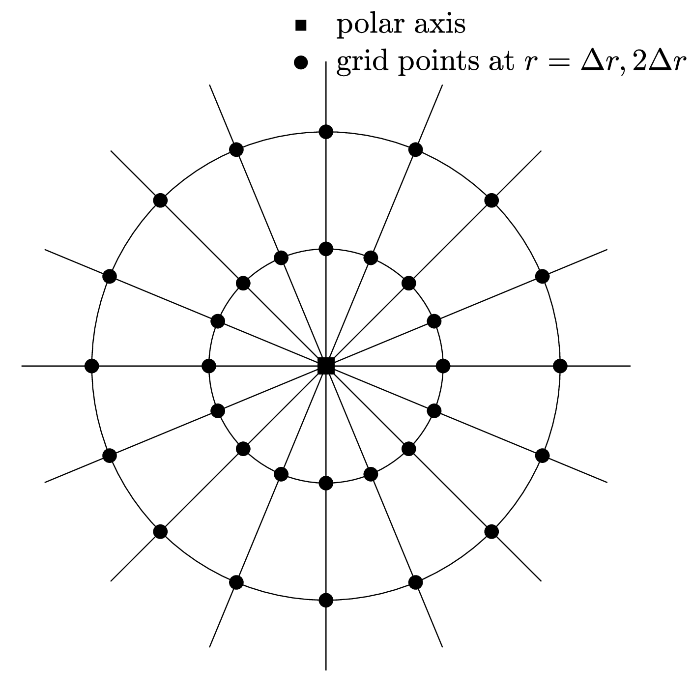
Figure 2: Predicting a scalar function at the polar axis by using the function’s average value on the neighbouring points.

Problems (i) and (ii) are solved above. The factor $r^{\lvert m\rvert}$ in Eq. (6) indicates that the numerical error of the low-order FDM near the pole may be serious; this is problem (iii) in numerically solving PDEs at the pole, especially when there are high $m$ components in the system. To illustrate this problem, we evaluate the numerical error in using central difference method to evaluate the $\partial_{r}\hat{g}_{m}$, with $\hat{g}_{m}(r)=r^{\lvert m\rvert}$.

$$\frac{\partial\hat{g}_{m}}{\partial r}=\frac{(r_{j}+\Delta r)^{\lvert m\rvert}-(r_{j}-\Delta r)^{\lvert m\rvert}}{2\Delta r}\approx\lvert m\rvert r_{j}^{\lvert m\rvert-1}+C_{\lvert m\rvert}^{3}\left(\frac{\Delta r}{r_{j}}\right)^{2}r_{j}^{\lvert m\rvert-1}.$$ (12)

The relative error is estimated to be

$$\eta=\frac{(m-1)(m-2)}{3!}\left(\frac{\Delta r}{r_{j}}\right)^{2},$$ (13)

which indicates that a larger $m$ will dramatically increase the $\eta$. Particularly, when $m>4$, the relative error at $r=r_{2}$ becomes $\eta>1$ and the numerical error is intolerable. To solve problem (iii), one way is to use the Pade schemes [9] to calculate the radial derivatives. However, the change from the explicit to the implicit scheme significantly reduces the computation efficiency by an order of $1/N_{r}$.

Here we propose that the mean value theorem can be generalized to solve problem (iii). Eq. (7) can be written as

$$\hat{g}_{m}(r)=r^{\lvert m\rvert}\left(A_{m0}+A_{m1}r^{2}+\cdots\right),$$ (14)

which can be numerically evaluated at $r_{j_{-}}$ and $r_{j_{+}}$ ($j_{+}=j_{-}+1$) as

$$\begin{cases}A_{m0}r^{\lvert m\rvert}_{j_{-}}+A_{m1}r^{\lvert m\rvert+2}_{j_{-}}=\hat{g}_{m}(r_{j_{-}}),\\ A_{m0}r^{\lvert m\rvert}_{j_{+}}+A_{m1}r^{\lvert m\rvert+2}_{j_{+}}=\hat{g}_{m}(r_{j_{+}}).\end{cases}$$ (15)

Using $\hat{g}(r_{j_{-}},\theta)$ and $\hat{g}(r_{j_{+}},\theta)$, one finds $\hat{g}_{m}(r_{-})$ and $\hat{g}_{m}(r_{+})$; using Eq. (15), one finds the coefficients in Eq. (14), which shall be used to predict $\hat{g}(r<r_{j_{-}},\theta)$. This method can be understood as the ”generalized mean value theorem”, and the mean value theorem is the $j_{-}=2$ case.

To solve problem (iii) by using the generalized mean value theorem, we solve the PDE by using the FDM when $r\geq r_{j_{-}}$, and the values of the function to be solved in the domain $r<r_{j_{-}}$ is predicted by Eq. (14). According to Eq. (13), the numerical error of the low-order FDM decreases quickly with $r$ increasing. Note that the truncation error of Eq. (14) quickly decreases when approaching the pole. Therefore, $j_{-}$ should be chosen to be large enough to keep a small FDM error and small enough to keep a small truncation error. In practice, for a system containing $m\leq 6$ components near the pole, $j_{-}=5$ can be chosen to find a good enough numerical solution, as will be discussed in Section 4.

3 Application in the gyrokientic simulation for a tokamak torus

In global GK codes, such as NLT [22], the field-aligned coordinates $\boldsymbol{X}=(\sqrt{\psi_{T}},\alpha,\theta)$ are used to improve the computational efficiency, with $\alpha=q\theta-\zeta$ and $q$ the safety factor. As is mentioned in Section 1, when $\psi_{T}\to 0$, $\sqrt{\psi_{T}}\propto r$, and there is no difference to discuss the radial series expansions shown in Eq. (7) in these coordinates. However, the $\theta$ direction is along with the field line, and the scalar function is not periodic in this direction. To implement the proposed method, a scalar function $h$ in the field-aligned coordinates, need to be transformed to the magnetic flux coordinates. For each toroidal mode $h_{n}$, the transformation is given as

$$\bar{h}_{n}(r,\theta)=h_{n}(r,\theta)e^{inq(r)\theta}.$$ (16)

$\bar{h}_{n}$ is periodic in the $\theta$ direction. According to Eq. (16), the mean value theorem in the field-aligned coordinates is given by

$$h_{n}(0,\theta)e^{inq(0)\theta}=\frac{4}{3}\sum_{k=1}^{N_{\theta}}h_{n}(r_{2},\theta_{k})e^{inq(r_{2})\theta_{k}}-\frac{1}{3}\sum_{k=1}^{N_{\theta}}h_{n}(r_{3},\theta_{k})e^{inq(r_{3})\theta_{k}}.$$ (17)

$h$ can refer to either the perturbed electrostatic potential $\delta\phi$ or the distribution function $F$, since the dependence of the scalar function on the phase space coordinates will not affect our discussion.

In the ITG simulation, the maximum $m$ near the magnetic axis is connected with the toroidal mode number $n$, since $m-nq$ is usually a small number. For the $n=0$ mode, $j_{-}=2$ in the generalized mean value theorem and the long-wavelength approximation in the quasi-neutrality equation are both appropriate. So, Eq. (17) predicts the distribution function at the magnetic axis in solving Eq. (1) and serves as a numerical inner boundary condition in solving Eq. (3). For $n>0$ modes, the long-wavelength approximation in the quasi-neutrality equation may not be appropriate near the magnetic axis. The generalized mean value method, in which $j_{-}$ is related to the maximum $m$, are used to predict the value of the function to be solved in the domain $r<r_{j_{-}}$ in solving Eq. (1) and Eq. (2).

The numerical treatment presented above are applied in NLT. In A and B, a Rosenbluth–Hinton (R-H) test and a set of linear ITG simulations away from the magnetic axis are presented as benchmarks for NLT using the new numerical treatment at the magnetic axis. It is worth pointing out that although the Vlasov equation in NLT is solved by the specific semi-Lagrangian method [22] combined with I-transform [23], the proposed method can also be applied to other Vlasov equation solvers in the framework of the FDM.

4 Numerical results near the magnetic axis

In this section, numerical results of the R-H test and the linear ITG simulation near the magnetic axis are presented for verification. Firstly, the $n=0$ R-H test with $j_{-}=2$ is presented. Then the GK simulation result of the $n>0$ ITG mode with different $j_{-}$ are presented.

4.1 R-H test

According to Ref. [24], an initial perturbed temperature will drive the electrostatic potential that balances it. This provides a convenient test for the radial force balance equation, which reads

$$\delta E_{r}+\delta u_{\theta}B_{T}-\delta u_{\zeta}B_{P}-\frac{\delta p^{\prime}_{i}}{n_{0}e_{i}}=0,$$ (18)

with $\delta E_{r}$ the perturbed radial electric field, $\delta u_{\theta}$ the perturbed poloidal flow, $\delta u_{\zeta}$ the perturbed toroidal flow, $B_{P}$ the poloidal magnetic field, $B_{T}$ the toroidal magnetic field, $\delta p_{i}=n_{0}\delta T_{i}$ and $\delta T_{i}$ the perturbed temperature. Here the prime represents the radial derivative. $\delta u_{\zeta}$, $\delta E_{r}$ and $\delta p_{i}$ are directly given by the simulation results, while the $\delta u_{\theta}$ is calculated from Eq. (18).

The simulation parameters are set as: $B_{0}=2.00\mathrm{T}$, the major radius $R_{0}=1.65\mathrm{m}$, the minor radius $a=0.40\mathrm{m}$. To avoid profile effects, the test is carried out in the radial homogeneous plasma, with equilibrium profiles $T_{0i}=1\mathrm{keV}$, $\tau_{e}\equiv T_{0e}/T_{oi}=1$, $n_{0}=10^{19}\mathrm{m}^{-3}$, $q=1.2$. The initial perturbed ion distribution function is given by

$$\delta f_{i}=\left(\frac{w}{T_{0i}}-\frac{3}{2}\right)\frac{\delta T_{i}}{T_{0i}}F_{0i},$$ (19)

with $w$ the kinetic energy, $F_{0i}$ the equilibrium ion distribution function set as a local Maxwellian distribution. Eq. (19) gives the initial source as an ion heating impulse without density and parallel momentum input. The initial perturbed temperature is set as

$$\frac{\delta T_{i}(r)}{T_{0i}}=1.7\times 10^{-3}\exp{\left(-\frac{r^{2}}{\Delta_{\delta T}^{2}}\right)},$$ (20)

with $\Delta_{\delta T}=0.25a$. The $\Delta_{\delta T}$ is large enough to make the radial structure of $\delta T_{i}$ wider than the banana width of a trapped particle whose velocity approaching $v_{ti}$ near the magnetic axis. Although $T_{0i}$ is radial homogeneous, $v_{ti}$ is defined as $v_{ti}=\sqrt{2T_{0i}(r_{0})/m_{i}}$, with $r_{0}=0$. The simulation results are shown in Fig. 3. It can be seen that the pressure gradient is well balanced with the radial electric field.

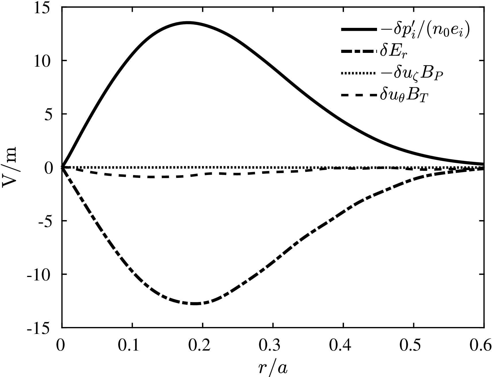
Figure 3: Different terms in the radial force balance equation.

4.2 Linear ITG simulation

The ITG mode tends to be more stable near the magnetic axis where the magnetic shear, $\hat{s}=\frac{q}{r}\frac{\mathrm{d}q}{\mathrm{d}r}$, is weaker. So, these tests are carried out with the internal transport barrier (ITB) like profiles for a relative high ITG growth rate near the magnetic axis. The main parameter are set as: $B_{0}=2.10\mathrm{T}$, $R_{0}=1.67\mathrm{m}$, $a=0.67\mathrm{m}$. Equilibrium profiles are based on the ITB data in DIII-D [25]. They are set as

$$q(r)=1.10+7.79\left(\frac{r}{a}\right)^{2}-17.71\left(\frac{r}{a}\right)^{3}+13.46\left(\frac{r}{a}\right)^{4},$$ (21a)

$$n_{0i}(r)=1.25-1.25\left(\frac{r}{a}\right)^{2}+0.50\left(\frac{r}{a}\right)^{3},$$ (21b)

$$T_{0i}(r)=-\frac{1}{2}\tanh{\left(\frac{r^{2}-r_{m}^{2}}{\Delta_{T}^{2}}\right)}+1,$$ (21c)

with $\Delta_{T}=0.15a$, $r_{m}=10^{-4}a$, $T_{0i}(r_{0})=3\mathrm{keV}$ and $n_{0i}(r_{0})=2\times 10^{19}\mathrm{m^{3}}$. Details of equilibrium profiles are shown in Fig. 4. Moreover, an equilibrium radial electric field $E_{0r}$ that balances the equilibrium pressure gradient is applied. The simulation domain are $r/a\in[0,0.9]$, $\theta\in[-\pi,\pi]$, $\alpha\in[0,2\pi]$, $v_{\parallel}/v_{ti}\in[3,3]$, $\mu B_{0}/T_{0i}(r_{0})=[0,9]$. Grid numbers are $\left(N_{r},N_{\alpha},N_{\theta},N_{v_{\parallel}},N_{\mu}\right)=(200,142,16,64,16)$. $\mu$ is discretized according to the Gauss-Legendre formula, while the other variables are discretized uniformly.

The mode structure of the toroidal mode $n=6$, which is one of the most unstable modes, on a minor cross section is shown in Fig. 5. It is a typical toroidal mode structure that balloons on the weak field side. On the strong field side, the balloon structure disappears and the amplitude of the mode is much weaker. The radial eigenfunctions of the $m/n=6/6$ harmonics $\lvert\delta\phi_{6,6}\rvert$ simulated by different $j_{-}$ near the magnetic axis are shown in Fig. 6. It can be seen that the $\lvert\delta\Phi_{6,6}\rvert=\lvert\delta\phi_{6,6}\rvert/r^{6}$ computed by using $j_{-}=3$ is not smooth. According to Eq. (13), the $\eta$ of the second-order FDM at $r_{j_{-}}$ ($j_{-}=3$) is estimate to be $\eta=83.8\%$. The severe numerical error here results in an inconsistency between the radial eigenfunction calculated and the radial series expansion used, which leads to the non-smooth $\lvert\delta\Phi_{6,6}\rvert$. The results computed by using $j_{-}=4,5$ tend to be smooth and convergent, which indicates that $\eta=20.8\%$ ($j_{-}=5$) is a appropriate choice for a good enough numerical solution near the magnetic axis. Although the $\lvert\delta\Phi_{6,6}\rvert$ computed by using $j_{-}=3$ is not as smooth as these computed by using $j_{-}=4,5$, the linear growth rates and real frequencies shown in Table 1 are almost the same. The loss of accuracy of the radial eigenfunction can hardly affect eigenvalues due to the reason that the eigenfunction itself is so small near the magnetic axis.

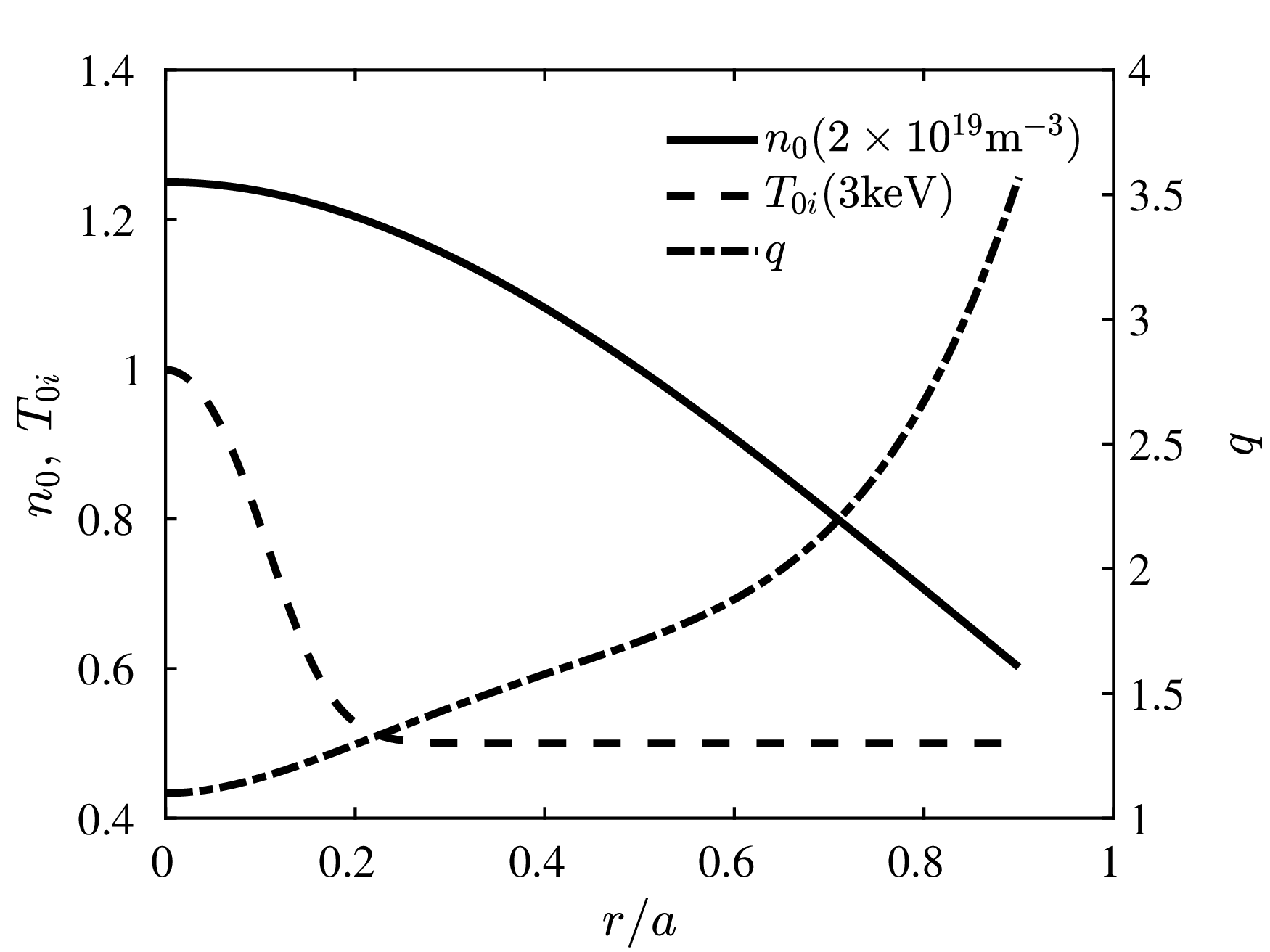
Figure 4: Equilibrium profiles used in the linear ITG simulation near the magnetic axis.

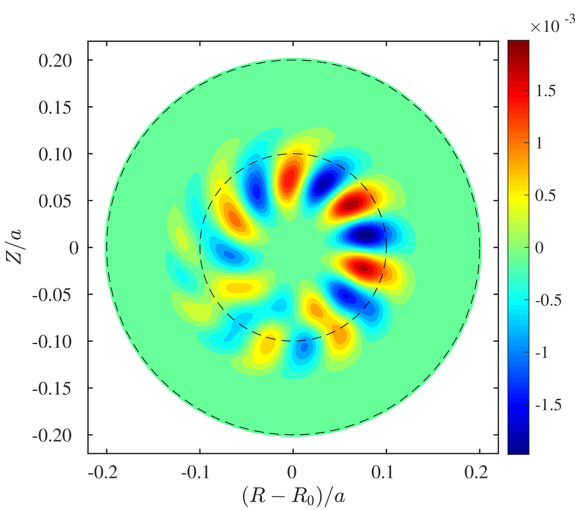
Figure 5: Mode structure of $\delta\phi$ with $n=6$.

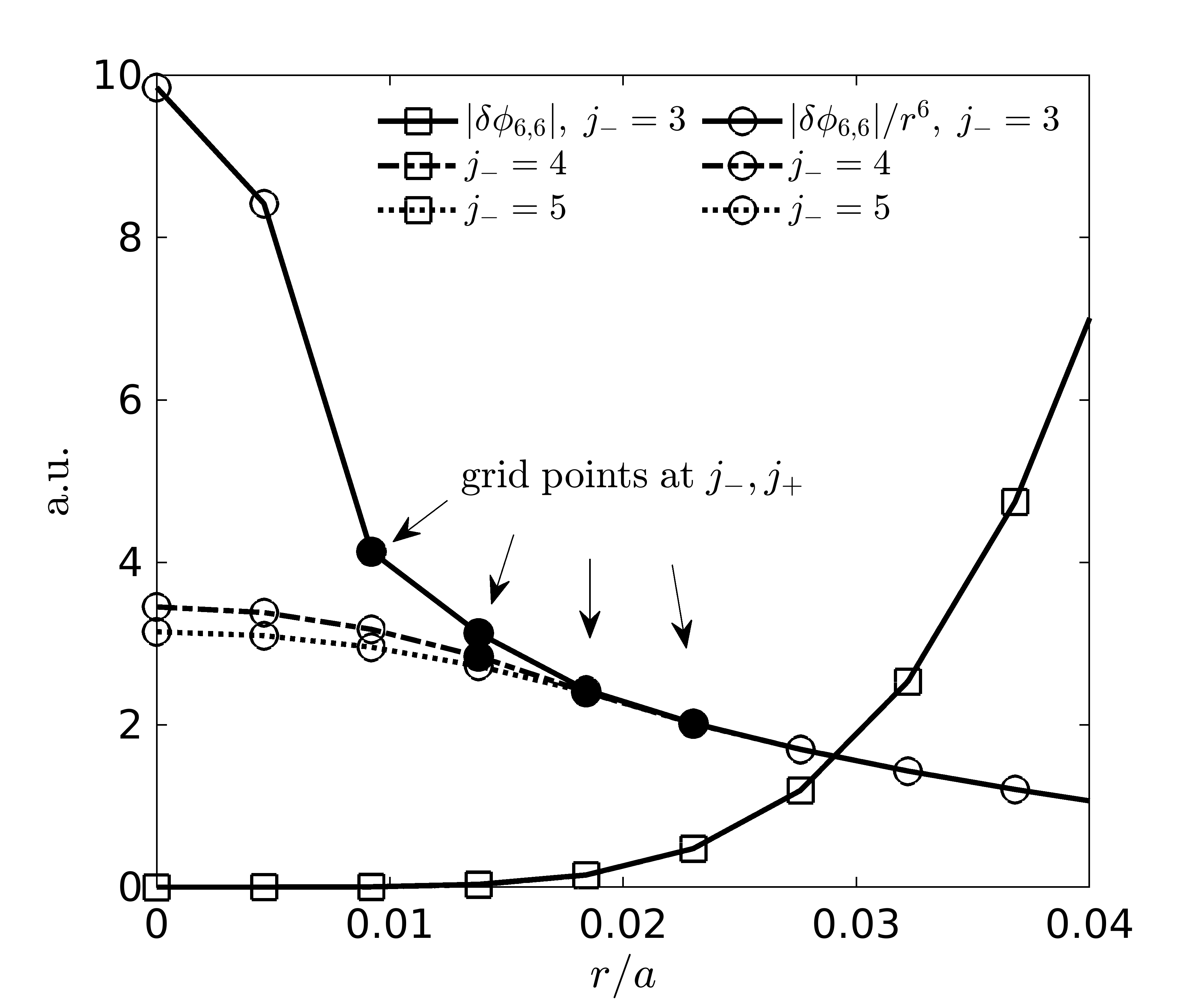
Figure 6: $\lvert\delta\phi_{6,6}\rvert$ computed by using different $j_{-}$; open squares: $\lvert\delta\phi_{6,6}\rvert$; open circles: $\lvert\delta\phi_{6,6}\rvert/r^{6}$; solid lines: using $j_{-}=3$; dotted-dashed lines: using $j_{-}=4$; dotted lines: using $j_{-}=5$.

$j_{-}$	$\gamma\;(R_{0}/v_{ti})$	$\omega\;(R_{0}/v_{ti})$	$\eta$ at $r_{j_{-}}$
3	0.219	$1.816$	$83.3\%$
4	0.219	$1.816$	$37.0\%$
5	0.219	$1.801$	$20.8\%$

Table 1: Linear growth rates, real frequencies and $\eta$ of the second-order FDM at $r_{j_{-}}$ computed by using different $j_{-}$.

5 Conclusion

We proposed a new computational method to solve the hyperbolic (Vlasov) equation coupled to the elliptic (Poisson-like) equation at the polar axis. We prove the mean value theorem, which indicates that the value of a scalar function at the polar axis is predicted by its neighbouring values based on the continuity condition. This continuity condition systematically solves the pole problems including the singular factor $1/r$ in the hyperbolic equation and the inner boundary in the elliptic equation. Moreover, the severe numerical error of low-order finite-difference schemes near the polar axis is mitigated by the generalized mean value theorem; the value of the scalar function to be solved in the domain $r<r_{j_{-}}$ is predicted by the values at $r_{j_{\pm}}$. The proposed method is applied in the global GK simulation. In the $n=0$ R-H test, $j_{-}=2$, and an initial perturbed temperature drives the electrostatic potential that balances it, which is consistent with the theoretical prediction. In the $n>0$ linear ITG simulation, convergent and smooth radial eigenfunctions are obtained by using $j_{-}=4,5$. In addition, the radial eigenfunction itself is so small near the magnetic axis that the loss of accuracy can hardly affect eigenvalues.

Appendix A R-H test away from the magnetic axis

The R-H test of NLT has been performed in Ref. [26, 22]. In this section, a R-H test away from the magnetic axis is performed as a benchmark for the NLT using the new computational method to treat the magnetic axis. Parameters are set as following: magnetic field at the axis $B_{0}=1.50\mathrm{T}$, major radius $R_{0}=1.25\mathrm{m}$, minor radius $a=0.45\mathrm{m}$. To avoid the phase mixing effect [27], the test is carried out in radial homogeneous plasma, with equilibrium profiles $q=1.2$, $T_{0i}=0.15\mathrm{keV}$, $\tau_{e}\equiv T_{0e}/T_{0i}=1$. The initial perturbation is given in the form of a radial perturbed density

$$\frac{\delta n_{i}(r)}{n_{0}(r)}=\begin{cases}10^{-5}\sin{\left(\frac{r-r_{a}}{r_{b}-r_{a}}\right)},\quad r\in\left[r_{a},r_{b}\right]\\ 0,\qquad\qquad\qquad\quad\quad\mathrm{else}\end{cases}$$ (22)

with $\delta n_{i}$ the perturbed density, $r_{a}=0.4a$, $r_{b}=0.6a$. The radial simulation domain is $[0,0.85a]$, which particularly includes the magnetic axis.

By taking account of the geodesic acoustic mode (GAM) oscillations, the collisionless damping and the residual flow [28], the $m=n=0$ component of perturbed radial electric field is expected to behave as

$$\frac{\delta E_{r}(t)}{\delta E_{r}(0)}=R_{F}+(1-R_{F})e^{-\gamma_{g}t}\cos{(\omega_{g}t)}$$ (23)

where $R_{F}=1/\left(1+1.6q^{2}/\sqrt{\epsilon}\right)$ is the residual flow, $\epsilon=r/R_{0}$ is inverse aspect-ratio, $\omega_{g}$ and $\gamma_{g}$ are theoretical frequency and damping rate [29, 30], respectively. Fig. 7 shows the time evolution of perturbed radial electric field at $r_{0}=0.5a$. The normalized unit of speed is defined as $v_{ti}=\sqrt{(2T_{0i}(r_{0})/m_{i})}$. The oscillation frequency, collisionless damping rate and residual flow all agree with the theoretical values.

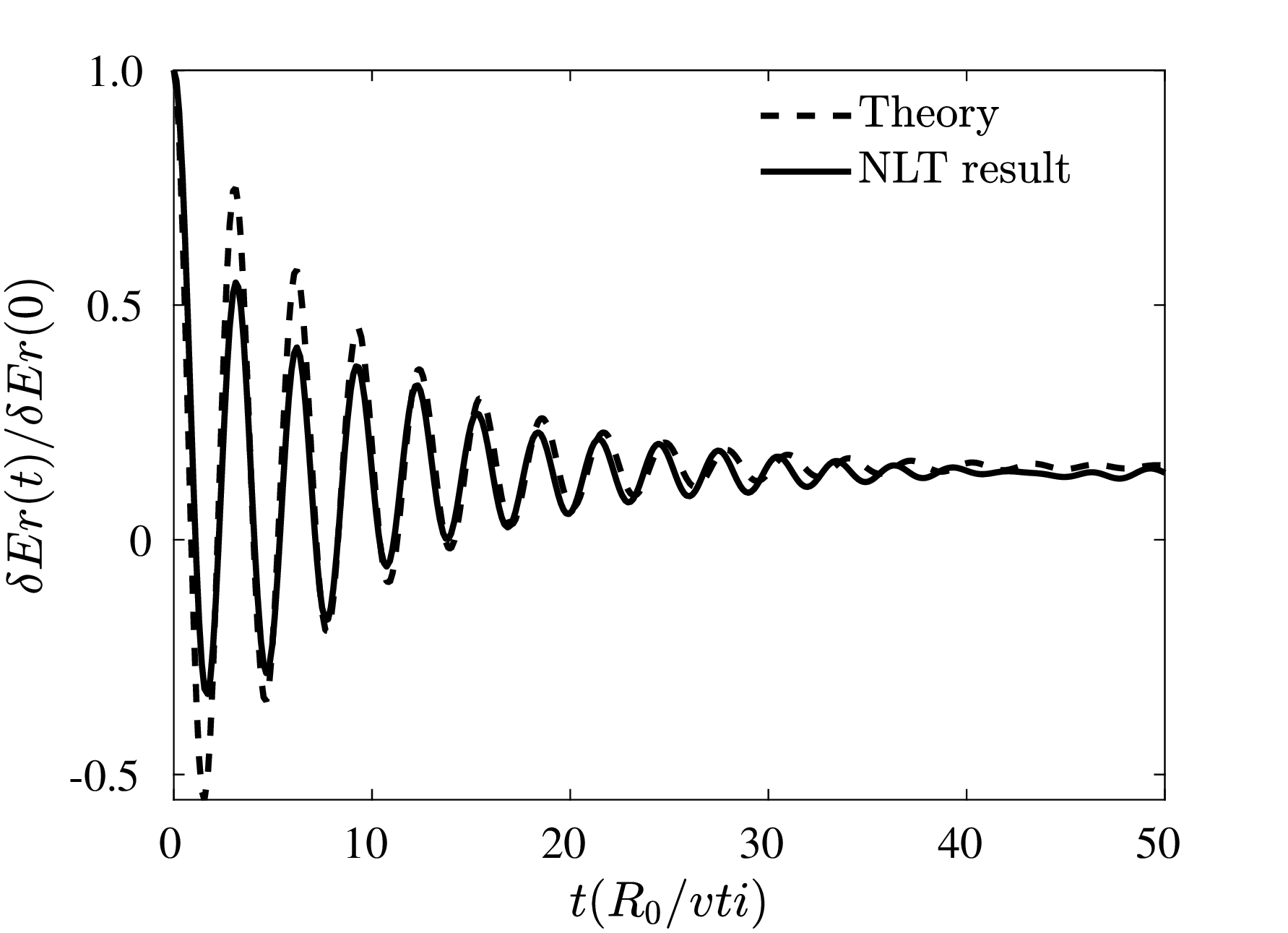
Figure 7: Time evolution of perturbed radial electric field at $r_{0}$

Appendix B Linear ITG simulations away from the magnetic axis

The linear ITG tests of NLT have been performed in Ref. [26, 22]. In this section, a set of linear ITG mode tests are performed to benchmark the NLT, which uses the new computational method to treat the magnetic axis, against another global GK code. These tests are carried out with the Cyclone Base Case (CBC) [31] parameters: $B_{0}=1.90\mathrm{T}$, $R_{0}=1.67\mathrm{m}$, $a=0.60\mathrm{m}$. The $q$ profile is set as

$$q(r)=0.854+2.4045\left(\frac{r}{a}\right)^{2}$$ (24)

with $q_{0}\equiv q(r_{0})=1.455$, $r_{0}=0.5$. The initial ion temperature and density profile are set as

$$\hat{A}(r)=\frac{A(r)}{A(r_{0})}=\exp{\left[-\kappa_{A}\frac{a}{R_{0}}\Delta_{A}\tanh{\left(\frac{r-r_{0}}{a}\right)}\right]},$$ (25)

where $A$ can be chosen as either $T_{0i}$ or $n_{0i}$, and $T_{0i}(r_{0})=1.97\mathrm{keV}$, $n_{0i}=10^{19}\mathrm{m^{3}}$, $\Delta_{A}=0.30$, $\kappa_{n}\equiv R_{0}/L_{n}=2.23$, $\kappa_{T}=6.96$. $L_{n}$ and $L_{T}$ are the scale length of density and ion temperature, respectively. Here, $\tau_{e}=1$ is assumed. A comparison of linear ITG frequency and growth rate between different codes are shown in Fig. 8. The dimensionless number $k_{\theta}\rho_{i}$ is used to represent the toroidal mode number, where $k_{\theta}$ is defined by $k_{\theta}=nq_{0}/r_{0}$. There are good agreements between simulation results of two codes.

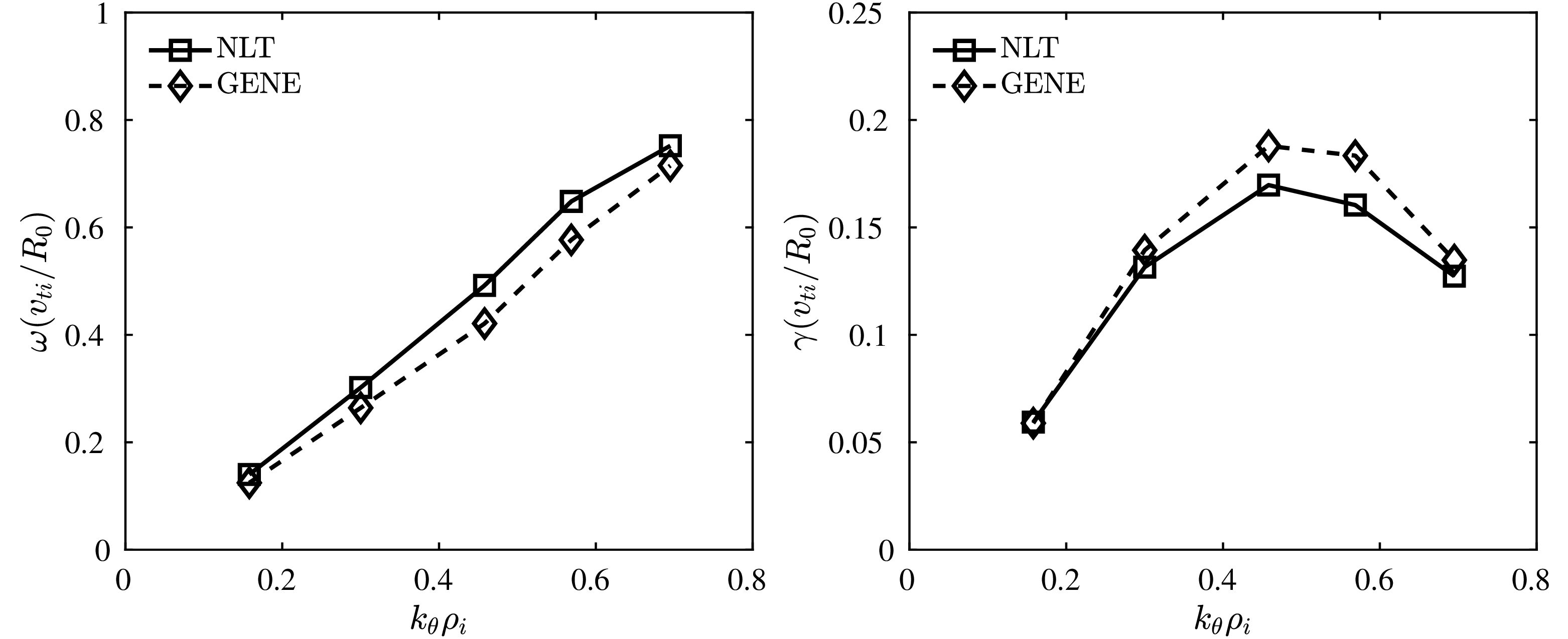
Figure 8: Comparison of linear ITG frequency (a) and growth rate (b) between GENE and NLT.

References

- [1] G. Constantinescu, S. Lele, A highly accurate technique for the treatment of flow equations at the polar axis in cylindrical coordinates using series expansions, J. Comput. Phys. 183 (2002) 165–186.
- [2] M. D. Griffin, E. Jones, J. D. Anderson, A computational fluid dynamic technique valid at the centerline for non-axisymmetric problems in cylindrical coordinates, J. Comput. Phys. 30 (1979) 352–360.
- [3] W. Huang, D. M. Sloan, Pole condition for singular problems: The pseudospectral approximation, J. Comput. Phys. 107 (1993) 254–261.
- [4] J. P. Boyd, Chebyshev and Fourier Spectral Methods, Springer Berlin, Heidelberg, 1989.
- [5] T. Matsushima, P. Marcus, A spectral method for polar coordinates, J. Comput. Phys. 120 (1995) 365–374.
- [6] W. Verkley, A spectral model for two-dimensional incompressible fluid flow in a circular basin, J. Comput. Phys. 136 (1997) 115–131.
- [7] B. Fornberg, A pseudospectral approach for polar and spherical geometries, SIAM J. Sci. Comp. 16 (1995) 1071–1081.
- [8] K. Mohseni, T. Colonius, Numerical treatment of polar coordinate singularities, J. Comput. Phys. 157 (2000) 787–795.
- [9] S. K. Lele, Compact finite difference schemes with spectral-like resolution, J. Comput. Phys. 103 (1992) 16–42.
- [10] S. Wang, Z. Wang, T. Wu, Self-organized evolution of the internal transport barrier in ion-temperature-gradient driven gyrokinetic turbulence, Phys. Rev. Lett. 132 (2024) 065106.
- [11] A. J. Brizard, T. S. Hahm, Foundations of nonlinear gyrokinetic theory, Rev. Mod. Phys. 79 (2007) 421–468.
- [12] W. W. Lee, Gyrokinetic approach in particle simulation, Phys. Fluids 26 (1983) 556–562.
- [13] Z. Lin, T. S. Hahm, W. W. Lee, W. M. Tang, R. B. White, Turbulent transport reduction by zonal flows: Massively parallel simulations, Science 281 (1998) 1835–1837.
- [14] J. Candy, R. Waltz, An eulerian gyrokinetic-maxwell solver, J. Comput. Phys. 186 (2003) 545–581.
- [15] V. Grandgirard, Y. Sarazin, X. Garbet, G. Dif‐Pradalier, P. Ghendrih, N. Crouseilles, G. Latu, E. Sonnendrücker, N. Besse, P. Bertrand, GYSELA, a full‐f global gyrokinetic Semi‐Lagrangian code for ITG turbulence simulations, AIP Conf. Proc. 871 (2006) 100–111.
- [16] S. Jolliet, A. Bottino, P. Angelino, R. Hatzky, T. Tran, B. Mcmillan, O. Sauter, K. Appert, Y. Idomura, L. Villard, A global collisionless pic code in magnetic coordinates, Comput. Phys. Comm. 177 (2007) 409–425.
- [17] Y. Idomura, M. Ida, T. Kano, N. Aiba, S. Tokuda, Conservative global gyrokinetic toroidal full-f five-dimensional vlasov simulation, Comput. Phys. Comm. 179 (2008) 391–403.
- [18] K. Obrejan, K. Imadera, J. Li, Y. Kishimoto, Development of a global toroidal gyrokinetic vlasov code with new real space field solver, Plasma Fusion Res. 10 (2015) 3403042–3403042.
- [19] H. Feng, W. Zhang, Z. Lin, X. Zhufu, J. Xu, J. Cao, D. Li, Development of finite element field solver in gyrokinetic toroidal code, Commun. Comput. Phys. 24 (2018) 655–671.
- [20] H. R. Lewis, P. M. Bellan, Physical constraints on the coefficients of Fourier expansions in cylindrical coordinates, J. Math. Phys. 31 (1990) 2592–2596.
- [21] H. Eisen, W. Heinrichs, K. Witsch, Spectral collocation methods and polar coordinate singularities, J. Comput. Phys. 96 (1991) 241–257.
- [22] L. Ye, X. Xiao, Y. Xu, Z. Dai, S. Wang, Implementation of field-aligned coordinates in a semi-lagrangian gyrokinetic code for tokamak turbulence simulation, Plasma Sci. Technol. 20 (2018) 074008.
- [23] S. Wang, Nonlinear scattering term in the gyrokinetic Vlasov equation, Phys. Plasmas 20 (2013) 082312.
- [24] S. Wang, Zonal flows driven by the turbulent energy flux and the turbulent toroidal Reynolds stress in a magnetic fusion torus, Phys. Plasmas 24 (2017) 102508.
- [25] K. H. Burrell, M. E. Austin, C. M. Greenfield, L. L. Lao, B. W. Rice, G. M. Staebler, B. W. Stallard, Effects of velocity shear and magnetic shear in the formation of core transport barriers in the diii-d tokamak, Plasma Phys. Control. Fusion 40 (1998) 1585.
- [26] Z. Dai, Y. Xu, L. Ye, X. Xiao, S. Wang, Gyrokinetic simulation of itg turbulence with toroidal geometry including the magnetic axis by using field-aligned coordinates, Comput. Phys. Comm. 242 (2019) 72–82.
- [27] F. Zonca, L. Chen, Radial structures and nonlinear excitation of geodesic acoustic modes, Euro. Phys. Lett. 83 (2008) 35001.
- [28] M. N. Rosenbluth, F. L. Hinton, Poloidal flow driven by ion-temperature-gradient turbulence in tokamaks, Phys. Rev. Lett. 80 (1998) 724–727.
- [29] H. Sugama, T.-H. Watanabe, Collisionless damping of geodesic acoustic modes, J. Plasma Phys. 72 (2006) 825–828.
- [30] H. Sugama, T.-H. Watanabe, Erratum: ‘collisionless damping of geodesic acoustic modes’ [j. plasma physics (2006) 72, 825], J. Plasma Phys. 74 (2008) 139 – 140.
- [31] A. M. Dimits, G. Bateman, M. A. Beer, B. I. Cohen, W. Dorland, G. W. Hammett, C. Kim, J. E. Kinsey, M. Kotschenreuther, A. H. Kritz, L. L. Lao, J. Mandrekas, W. M. Nevins, S. E. Parker, A. J. Redd, D. E. Shumaker, R. Sydora, J. Weiland, Comparisons and physics basis of tokamak transport models and turbulence simulations, Phys. Plasmas 7 (2000) 969–983.