Operator SVD with Neural Networks
via Nested Low-Rank Approximation

Abstract

Computing eigenvalue decomposition (EVD) of a given linear operator, or finding its leading eigenvalues and eigenfunctions, is a fundamental task in many machine learning and scientific computing problems. For high-dimensional eigenvalue problems, training neural networks to parameterize the eigenfunctions is considered as a promising alternative to the classical numerical linear algebra techniques. This paper proposes a new optimization framework based on the low-rank approximation characterization of a truncated singular value decomposition, accompanied by new techniques called nesting for learning the top-$L$ singular values and singular functions in the correct order. The proposed method promotes the desired orthogonality in the learned functions implicitly and efficiently via an unconstrained optimization formulation, which is easy to solve with off-the-shelf gradient-based optimization algorithms. We demonstrate the effectiveness of the proposed optimization framework for use cases in computational physics and machine learning.

1 Introduction

Spectral decomposition techniques, including singular value decomposition (SVD) and eigenvalue decomposition (EVD), are crucial tools in machine learning and data science for handling large datasets and reducing their dimensionality while preserving prominent structures; see, e.g., [1, 2]. They break down a matrix (or a linear operator) into its constituent parts, enabling a better understanding of the underlying geometry and relationships within the data. These form the foundation of various low-dimensional embedding algorithms [3, 4, 5, 6, 7, 8, 9, 10] and correlation analysis algorithms [11, 12] and are widely used in image and signal processing [13, 14, 15, 16, 17], natural language processing [18, 19], among other fields. Beyond machine learning applications, solving eigenvalue problems is a crucial step in solving partial differential equations (PDEs), such as Schrödinger’s equations in quantum chemistry [20, 21].

The standard approach to these problems in practice is to perform the matrix spectral decomposition using the standard techniques from numerical linear algebra [22]. In machine learning, the size of the matrix is typically given by the size of the data sample. In physical simulation, the underlying matrix scales with the resolution of discretization of a given domain. In general, the full eigendecomposition of a matrix can be performed in $O(N^{3})$ time complexity if the matrix can be stored in memory. For large matrices, iterative subspace methods can efficiently find top eigenmodes via repeating matrix-vector products [22]. For large-scale, high-dimensional data, however, the memory, computational, and statistical complexity of matrix decomposition algorithms poses a significant challenge in practice. As the data size (or the resolution of the grid in physical simulation) or the dimensionality of the underlying problem increases, the matrix-based approach becomes easily infeasible as simply storing the eigenvectors in memory is too costly.

A promising alternative is to approximate the singular- or eigen-functions using parametric function approximators, assuming that there exists an abstract operator that induces a target matrix to decompose. In other words, we aim to approximate an eigenvector $\hat{\boldsymbol{\phi}}_{\ell}\in\mathbb{R}^{N}$ by a single parametric function $\hat{\phi}_{\ell}\mathchoice{\colon}{\colon}{\mathchar 58\relax\mspace{1.0mu}}{\mathchar 58\relax}\mathcal{X}\to\mathbb{R}$. In Fig. 1, we illustrate our framework NeuralSVD, which is a special instance of the parametric approach, as a schematic diagram. Unlike the nonparametric approach which relies on the Nyström method [23, 24] to extrapolate eigenvectors to unseen points, the parametric eigenfunctions can naturally extrapolate without the storage and computational complexity of Nyström; refer to Sec. A.1 for a detailed discussion. Furthermore, given the exceptional ability of neural networks (NNs) to generalize with complex data, such as convolutional neural networks for images, transformers for natural language, and recently developed NN ansatzes for quantum chemistry [20, 21], one can anticipate better extrapolation performance than in the nonparametric, matrix approach. In the context of solving PDEs, the parametric approach stands out, notably because it necessitates only a sampler from a specified domain without the need for discretization. This is particularly advantageous as it helps mitigate the potential introduction of undesirable approximation errors.

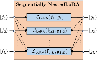
(a)

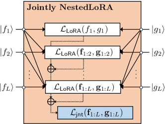
(b)

Figure 2: Schematic illustrations of the nesting techniques; recall Fig. 1. The operator and data (and weights for the joint nesting) are omitted for simplicity. In both cases, gradients are computed and backpropagated from the blue boxes. Gradients cannot be backpropagated through the dashed lines in (a); see Sec. 3.2 for the details.

In this paper, we propose a new optimization framework that can train neural networks to approximate the top-$L$ orthogonal singular- (or eigen-) functions of an operator. The proposed method is based on an unconstrained optimization problem from Schmidt’s low-rank approximation theorem (1907) that admits a naturally unbiased gradient estimator. To learn the ordered top-$L$ orthogonal singular basis as the optimal solution simultaneously, we introduce new techniques called nesting to break the symmetry so that we can learn the singular functions in the order of singular values; see the high-level illustrations in Fig. 2.

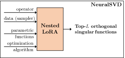
Figure 1: Schematic illustration of NeuralSVD.

While several frameworks have been proposed in the machine learning community to systematically recover ordered eigenfunctions using neural networks [26, 27], these approaches encounter practical optimization challenges, particularly in enforcing the orthonormality of the learned eigenfunctions. Compared to the prior works, our framework can (1) learn the top-$L$ orthogonal singular bases more efficiently for larger $L$ due to the more stable optimization procedure, and (2) perform SVD of a non-self-adjoint operator by design, handling EVD of a self-adjoint operator as a special case. We demonstrate the power of our framework in solving PDEs and representation learning for cross-domain retrieval.

2 Problem Setting and Preliminaries

2.1 Operator SVD

While SVD is typically assumed to be done via EVD, our low-rank approximation framework can directly perform SVD, handling EVD as a special case. We consider two separable Hilbert spaces $\mathcal{F}$ and $\mathcal{G}$ and a linear operator $\mathpzc{T}\mathchoice{\colon}{\colon}{\mathchar 58\relax\mspace{1.0mu}}{\mathchar 58\relax}\mathcal{F}\to\mathcal{G}$. We will use the bra-ket notation, which denotes $\mathchoice{\mspace{1.0mu}|\mspace{1.0mu}}{|}{|}{|}f\rangle$ for a function $f(\cdot)$ throughout, as it allows us to describe the proposed method in a succinct way. For most applications, the Hilbert spaces $\mathcal{F}$ and $\mathcal{G}$ are $\mathscr{L}^{2}$ spaces of square-integrable functions, and a reader thus can read the inner product between two real-valued functions $\langle f\mathchoice{\mspace{1.0mu}|\mspace{1.0mu}}{|}{|}{|}f^{\prime}\rangle$ as an integral $\int_{\mathcal{X}}f(x)f^{\prime}(x)\mu(\mathop{}\!\mathrm{d}x)$ for some underlying measure $\mu$ over a domain $\mathcal{X}$. In learning problems, $\mathpzc{T}$ is typically an integral kernel operator induced by a kernel function, accompanied by data distributions as the underlying measures. In solving PDEs, $\mathpzc{T}$ is given as a differential operator that governs a physical system of interest, where the underlying measure is the Lebesgue measure over a domain.

For a compact operator $\mathpzc{T}$, it is well known that there exist orthonormal bases $(\phi_{i})_{i\geq 1}$ and $(\psi_{i})_{i\geq 1}$ with a sequence of non-increasing, non-negative real numbers $(\sigma_{i})_{i\geq 1}$ such that $(\mathpzc{T}\phi_{i})(y)=\sigma_{i}\psi_{i}(y)$, $(\mathpzc{T}^{*}\psi_{i})(x)=\sigma_{i}\phi_{i}(x)$, $i=1,2,\ldots$. The function pairs $(\phi_{i},\psi_{i})$ are called (left- and right-, resp.) singular functions corresponding to the singular value $\sigma_{i}$. Hence, the compact operator $\mathpzc{T}$ can be written as

$$\mathpzc{T}=\sum_{i=1}^{\infty}\sigma_{i}\mathchoice{\mspace{1.0mu}|\mspace{1.0mu}}{|}{|}{|}\psi_{i}\rangle\langle\phi_{i}\mathchoice{\mspace{1.0mu}|\mspace{1.0mu}}{|}{|}{|},$$ (1)

for $\sigma_{1}\geq\sigma_{2}\geq\ldots\geq 0$, which we call the SVD of $\mathpzc{T}$. Here, $\mathchoice{\mspace{1.0mu}|\mspace{1.0mu}}{|}{|}{|}\psi\rangle\langle\phi\mathchoice{\mspace{1.0mu}|\mspace{1.0mu}}{|}{|}{|}\mathchoice{\colon}{\colon}{\mathchar 58\relax\mspace{1.0mu}}{\mathchar 58\relax}\mathcal{F}\to\mathcal{G}$ is the operator defined as $(\mathchoice{\mspace{1.0mu}|\mspace{1.0mu}}{|}{|}{|}\psi\rangle\langle\phi\mathchoice{\mspace{1.0mu}|\mspace{1.0mu}}{|}{|}{|})\mathchoice{\mspace{1.0mu}|\mspace{1.0mu}}{|}{|}{|}f\rangle\mathrel{\mathop{\mathchar 58\relax missing}}=(\langle\phi\mathchoice{\mspace{1.0mu}|\mspace{1.0mu}}{|}{|}{|}f\rangle)\mathchoice{\mspace{1.0mu}|\mspace{1.0mu}}{|}{|}{|}\psi\rangle$, which can be understood as an outer product.

2.2 EVD as a Special Case of SVD

In several applications, the operator is self-adjoint (i.e., $\mathpzc{T}^{*}=\mathpzc{T}$ with $\mathcal{F}=\mathcal{G}$), and sometimes even positive definite (PD). By the spectral theorem, a compact self-adjoint operator has the EVD of the form $\mathpzc{T}=\sum_{i=1}^{\infty}\lambda_{i}\mathchoice{\mspace{1.0mu}|\mspace{1.0mu}}{|}{|}{|}\phi_{i}\rangle\langle\phi_{i}\mathchoice{\mspace{1.0mu}|\mspace{1.0mu}}{|}{|}{|}$. In this case, the singular values of the operator are the absolute values of its eigenvalues, and for each $i$, the $i$-th left- and right- singular functions are either identical (if $\lambda_{i}\geq 0$) or only different by the sign (if $\lambda_{i}<0$). Hence, in particular, we can find its EVD by SVD in the case of a positive-definite (PD) operator. We remark in passing that our framework is also applicable for a certain class of non-compact operators; see Sec. 4.1 and Sec. D.6.

2.3 SpIN and NeuralEF

As alluded to earlier, Spectral Inference Networks (SpIN) [26] and Neural Eigenfunctions (NeuralEF) [27] are the most closely related prior works to ours, in the sense that these methods aim to learn the top-$L$ orthonormal parametric eigenbasis of a self-adjoint operator. Though there exist other approaches that aim to find beyond the top mode (or the ground state) in computational physics, most, if not all, approaches are based on ad-hoc regularization terms and are not guaranteed to systematically recover the top-$L$ ordered eigenfunctions. Hence, we focus on comparing SpIN and NeuralEF in the main text, and discuss the other literature and the two methods in greater details in Sec. B.

Since SpIN and NeuralEF are only applicable for self-adjoint operators, we temporarily assume a self-adjoint operator $\mathpzc{T}\mathchoice{\colon}{\colon}{\mathchar 58\relax\mspace{1.0mu}}{\mathchar 58\relax}\mathcal{F}\to\mathcal{F}$ in the rest of this section. SpIN and NeuralEF are both grounded in the principle of maximizing the Rayleigh quotient with orthonormality constraints. However, their optimization frameworks encounter nontrivial complexity issues, as summarized in Table 2. The primary challenge lies in efficiently handling these orthonormality constraints. To achieve fast convergence with off-the-shelf gradient-based optimization algorithms, it is also crucial to estimate gradients in an unbiased manner.

SpIN starts from the following variational characterization of the top-$L$ orthonormal eigenbasis:

$$\begin{aligned} \underset{\begin{subarray}{c}\tilde{\phi}_{\ell}\in\mathcal{F},\,\ell\in[L]\end{subarray}}{\text{maximize~{}~{}}}&\langle\tilde{\phi}_{\ell}\mathchoice{\mspace{1.0mu}|\mspace{1.0mu}}{|}{|}{|}\mathpzc{T}\tilde{\phi}_{\ell}\rangle\\ \text{subject~{}to~{}~{}}&\langle\tilde{\phi}_{i}\mathchoice{\mspace{1.0mu}|\mspace{1.0mu}}{|}{|}{|}\tilde{\phi}_{i^{\prime}}\rangle=\delta_{ii^{\prime}}\quad\forall 1\leq i,i^{\prime}\leq L.\end{aligned}$$ (2)

Since this formulation only captures the subspace without order, SpIN employs a special gradient masking scheme to learn the eigenfunctions in the correct order. The resulting algorithm involves Cholesky decomposition of $L\times L$ matrix per iteration, which takes $O(L^{3})$ complexity in general. Further, to work with unbiased gradient estimates, it requires a hyperparameter-sensitive bi-level optimization and necessitates the need to store the Jacobian of the parametric model. As a result, the unfavorable scalability with $L$, along with memory complexity and implementation challenges, reduces the practical utility of SpIN.

To circumvent the issues with SpIN, NeuralEF adopted and extended an optimization framework of EigenGame [28], which is a game-theoretic formulation for streaming PCA. The underlying optimization problem can be understood as a variant of the sequential version of the subspace characterization (2); see Sec. B.2.2 and (15) therein. The resulting optimization, however, still suffers from its biased gradient estimation, and requires the parametric functions to be normalized, i.e., needs to ensure $\|\hat{\phi}_{\ell}\|_{2}=\langle\hat{\phi}_{\ell}\mathchoice{\mspace{1.0mu}|\mspace{1.0mu}}{|}{|}{|}\hat{\phi}_{\ell}\rangle^{1/2}=1$ for every $\ell$. While the biased gradient could be alleviated via its simple variant, our experiments show that the function normalization step may slow down the convergence in practice; we defer the detailed discussion to Sec. B.2.2.

3 SVD via Nested Low-Rank Approximation

In what follows, we propose a new optimization-based algorithm for SVD with neural networks, based on Schmidt’s approximation theorem combined with new techniques called nesting for learning the singular functions in order. The resulting framework is significantly conceptually simpler and easier to implement than prior methods, without requiring sophisticated optimization techniques. Further, unlike SpIN and NeuralEF, we can directly perform the SVD of a non-self-adjoint operator. Hereafter, we assume that $\mathpzc{T}$ has $\{(\sigma_{\ell},\mathchoice{\mspace{1.0mu}|\mspace{1.0mu}}{|}{|}{|}\phi_{\ell}\rangle,\mathchoice{\mspace{1.0mu}|\mspace{1.0mu}}{|}{|}{|}\psi_{\ell}\rangle)\}_{\ell=1}^{\infty}$ as its orthonormal singular triplets.

3.1 Learning Subspaces via Low-Rank Approximation

Let $L$ be the number of modes we wish to retrieve. We will use a shorthand notation ${\bf f}_{1\mathchar 58\relax\ell}(x)\mathrel{\mathop{\mathchar 58\relax missing}}=[f_{1}(x),\ldots,f_{\ell}(x)]^{\intercal}$. Below, we will employ distinct variables $\mathchoice{\mspace{1.0mu}|\mspace{1.0mu}}{|}{|}{|}f\rangle$ and $\mathchoice{\mspace{1.0mu}|\mspace{1.0mu}}{|}{|}{|}g\rangle$ as counterparts to $\mathchoice{\mspace{1.0mu}|\mspace{1.0mu}}{|}{|}{|}\phi\rangle$ and $\mathchoice{\mspace{1.0mu}|\mspace{1.0mu}}{|}{|}{|}\psi\rangle$, respectively, which represent normalized singular functions. The intentional use of separate variables $\mathchoice{\mspace{1.0mu}|\mspace{1.0mu}}{|}{|}{|}f\rangle$ and $\mathchoice{\mspace{1.0mu}|\mspace{1.0mu}}{|}{|}{|}g\rangle$ underscores their role in representing scaled singular functions rather than normalized ones within our framework. The importance of this distinction will become apparent in the following subsection.

For the top-$L$ SVD of a given operator $\mathpzc{T}$, we consider the low-rank approximation (LoRA) objective defined as

$$\mathcal{L}_{\mathsf{LoRA}}({\bf f}_{1\mathchar 58\relax L},{\bf g}_{1\mathchar 58\relax L})\mathrel{\mathop{\mathchar 58\relax missing}}=\mathcal{L}_{\mathsf{LoRA}}({\bf f}_{1\mathchar 58\relax L},{\bf g}_{1\mathchar 58\relax L};\mathcal{T})\mathrel{\mathop{\mathchar 58\relax missing}}=-2\sum_{\ell=1}^{L}\langle g_{\ell}\mathchoice{\mspace{1.0mu}|\mspace{1.0mu}}{|}{|}{|}\mathpzc{T}f_{\ell}\rangle+\sum_{\ell=1}^{L}\sum_{\ell^{\prime}=1}^{L}\langle f_{\ell}\mathchoice{\mspace{1.0mu}|\mspace{1.0mu}}{|}{|}{|}f_{\ell^{\prime}}\rangle\langle g_{\ell}\mathchoice{\mspace{1.0mu}|\mspace{1.0mu}}{|}{|}{|}g_{\ell^{\prime}}\rangle.$$ (3)

This objective can be derived as the approximation error of $\mathpzc{T}$ via a low-rank expansion $\sum_{\ell=1}^{L}\mathchoice{\mspace{1.0mu}|\mspace{1.0mu}}{|}{|}{|}f_{\ell}\rangle\langle g_{\ell}\mathchoice{\mspace{1.0mu}|\mspace{1.0mu}}{|}{|}{|}$ measured in the squared Hilbert–Schmidt norm, for a compact operator $\mathpzc{T}$. We defer its derivation to Sec. D.1. By Schmidt’s LoRA theorem [25], which is the operator counterpart of Eckart and Young [29] for matrices, $({\bf f}^{\star},{\bf g}^{\star})$ corresponds to the rank-$L$ approximation of $\mathpzc{T}$. The proof of the following theorem can be found in Sec. D.2.

Theorem 1.

Assume that $\mathpzc{T}\mathchoice{\colon}{\colon}{\mathchar 58\relax\mspace{1.0mu}}{\mathchar 58\relax}\mathcal{F}\to\mathcal{G}$ is compact. Let $((f_{\ell}^{\star},g_{\ell}^{\star}))_{\ell=1}^{L}\in(\mathcal{F}\times\mathcal{G})^{L}$ be a global minimizer of $\mathcal{L}_{\mathsf{LoRA}}({\bf f}_{1\mathchar 58\relax L},{\bf g}_{1\mathchar 58\relax L})$. If $\sigma_{L}>\sigma_{L+1}$, then $\sum_{\ell=1}^{L}\mathchoice{\mspace{1.0mu}|\mspace{1.0mu}}{|}{|}{|}g_{\ell}^{\star}\rangle\langle f_{\ell}^{\star}\mathchoice{\mspace{1.0mu}|\mspace{1.0mu}}{|}{|}{|}=\sum_{\ell=1}^{L}\sigma_{\ell}\mathchoice{\mspace{1.0mu}|\mspace{1.0mu}}{|}{|}{|}\psi_{\ell}\rangle\langle\phi_{\ell}\mathchoice{\mspace{1.0mu}|\mspace{1.0mu}}{|}{|}{|}.$

In cases of degeneracy, i.e., when multiple singular functions share the same singular value, a minimizer will still recover a subspace spanned by the singular functions associated with that particular singular value. Throughout, we will assume such strict spectral gap assumptions for the sake of simple exposition.

3.2 Nesting for Learning Ordered Singular Functions

While the LoRA characterization of the spectral subspaces is favorable in practice due to its unconstrained nature, a global minimizer only characterizes the top-$L$ singular subspaces; note that $(\mathsf{Q}{\bf f}^{\star},\mathsf{Q}{\bf g}^{\star})$ for any orthogonal matrix $\mathsf{Q}\in\mathbb{R}^{L\times L}$ is also a global minimizer. We thus require an additional technique to find the singular functions and singular values in order by breaking the symmetry in the objective $\mathcal{L}_{\mathsf{LoRA}}({\bf f}_{1\mathchar 58\relax L},{\bf g}_{1\mathchar 58\relax L})$.

The idea for learning the ordered solution is as follows. Suppose that we can find a common global minimizer $({\bf f}_{1\mathchar 58\relax L}^{\star},{\bf g}_{1\mathchar 58\relax L}^{\star})$ of the objectives $\mathcal{L}_{\mathsf{LoRA}}({\bf f}_{1\mathchar 58\relax\ell},{\bf g}_{1\mathchar 58\relax\ell})$ for $1\leq\ell\leq L$. Then, from the optimality in Theorem 1, $\sum_{\ell=1}^{L}\mathchoice{\mspace{1.0mu}|\mspace{1.0mu}}{|}{|}{|}g_{\ell}^{\star}\rangle\langle f_{\ell}^{\star}\mathchoice{\mspace{1.0mu}|\mspace{1.0mu}}{|}{|}{|}$ must be the rank-$\ell$ approximation of $\mathpzc{T}$, which is $\sum_{\ell=1}^{L}\sigma_{\ell}\mathchoice{\mspace{1.0mu}|\mspace{1.0mu}}{|}{|}{|}\psi_{\ell}\rangle\langle\phi_{\ell}\mathchoice{\mspace{1.0mu}|\mspace{1.0mu}}{|}{|}{|}$. By telescoping, we then have $\mathchoice{\mspace{1.0mu}|\mspace{1.0mu}}{|}{|}{|}g_{\ell}^{\star}\rangle\langle f_{\ell}^{\star}\mathchoice{\mspace{1.0mu}|\mspace{1.0mu}}{|}{|}{|}=\sigma_{\ell}\mathchoice{\mspace{1.0mu}|\mspace{1.0mu}}{|}{|}{|}\psi_{\ell}\rangle\langle\phi_{\ell}\mathchoice{\mspace{1.0mu}|\mspace{1.0mu}}{|}{|}{|}$ for each $\ell\in[L]$, which is the desired, ordered solution. Since the optimization is performed with a certain nested structure, we call this idea nesting.

We remark that, unlike most existing methods that aim to directly learn ortho-normal eigenfunctions, the global optimum with (nested) LoRA characterizes the correct singular functions scaled by the singular value $\sigma_{\ell}$, as alluded to earlier. Using this property, one can estimate $\sigma_{\ell}$ by computing the product of norms $\|f_{\ell}^{\star}\|\cdot\|g_{\ell}^{\star}\|$; see Sec. E.5 for the detail.

Below, we introduce two different versions that implement this idea. The first version, called sequential nesting, is ideal when each eigenfunction is parameterized by separate neural networks. The second version, which we call joint nesting, can be used even when they are parameterized by a single network.

3.2.1 Sequential Nesting

Sequential nesting is based on the following observation: if $({\bf f}_{1\mathchar 58\relax\ell-1},{\bf g}_{1\mathchar 58\relax\ell-1})$ already captures the top-$(\ell-1)$ singular subspaces as a minimizer of $\mathcal{L}_{\mathsf{LoRA}}({\bf f}_{1\mathchar 58\relax\ell-1},{\bf g}_{1\mathchar 58\relax\ell-1})$, minimizing $\mathcal{L}_{\mathsf{LoRA}}({\bf f}_{1\mathchar 58\relax\ell},{\bf g}_{1\mathchar 58\relax\ell})$ for $(f_{\ell},g_{\ell})$ finds the $\ell$-th singular functions. Its proof can be found in Sec. D.3. Formally:

Theorem 2.

Assume that $\mathpzc{T}\mathchoice{\colon}{\colon}{\mathchar 58\relax\mspace{1.0mu}}{\mathchar 58\relax}\mathcal{F}\to\mathcal{G}$ is compact. Pick any $\ell\geq 1$. Let $({\bf f}_{\ell}^{\dagger},{\bf g}_{\ell}^{\dagger})\in\mathcal{F}\times\mathcal{G}$ be a global minimizer of $\mathcal{L}_{\mathsf{LoRA}}({\bf f}_{1\mathchar 58\relax\ell},{\bf g}_{1\mathchar 58\relax\ell})$, where $\sum_{i=1}^{\ell-1}\mathchoice{\mspace{1.0mu}|\mspace{1.0mu}}{|}{|}{|}g_{i}\rangle\langle f_{i}\mathchoice{\mspace{1.0mu}|\mspace{1.0mu}}{|}{|}{|}=\sum_{i=1}^{\ell-1}\sigma_{i}\mathchoice{\mspace{1.0mu}|\mspace{1.0mu}}{|}{|}{|}\psi_{i}\rangle\langle\phi_{i}\mathchoice{\mspace{1.0mu}|\mspace{1.0mu}}{|}{|}{|}$. If $\sigma_{\ell}>\sigma_{\ell+1}$, then $\mathchoice{\mspace{1.0mu}|\mspace{1.0mu}}{|}{|}{|}g_{\ell}^{\dagger}\rangle\langle f_{\ell}^{\dagger}\mathchoice{\mspace{1.0mu}|\mspace{1.0mu}}{|}{|}{|}=\sigma_{\ell}\mathchoice{\mspace{1.0mu}|\mspace{1.0mu}}{|}{|}{|}\psi_{\ell}\rangle\langle\phi_{\ell}\mathchoice{\mspace{1.0mu}|\mspace{1.0mu}}{|}{|}{|}$.

We can implement this idea by updating the iterate $(f_{\ell}^{(t)},g_{\ell}^{(t)})$ at time step $t\geq 1$ for each $\ell\in[L]$ aiming to minimize $\mathcal{L}_{\mathsf{LoRA}}({\bf f}_{1\mathchar 58\relax\ell}^{(t)},{\bf g}_{1\mathchar 58\relax\ell}^{(t)})$, regarding $({\bf f}_{1\mathchar 58\relax\ell-1}^{(t)},{\bf g}_{1\mathchar 58\relax\ell-1}^{(t)})$ as a good proxy to the global optimum. That is, for each $\ell\in[L]$,

$$(f_{\ell}^{(t+1)},g_{\ell}^{(t+1)})\leftarrow\mathsf{Opt}((f_{\ell}^{(t)},g_{\ell}^{(t)}),\mathop{}\!\partial_{{(f_{\ell},g_{\ell})}}\mathcal{L}_{\mathsf{LoRA}}({\bf f}_{1\mathchar 58\relax\ell}^{(t)},{\bf g}_{1\mathchar 58\relax\ell}^{(t)})).$$ (4)

Here, $\mathsf{Opt}(\boldsymbol{\theta},{\bf g})$ denotes a gradient-based optimization algorithm that returns the next iterate based on the current iterate $\boldsymbol{\theta}$ and the gradient ${\bf g}$.

Suppose that each model pair $(f_{\ell},g_{\ell})$ is parameterized via $L$ separate models with (disjoint) parameters $\theta=(\theta_{\ell})_{\ell=1}^{L}$. In this case, the $\ell$-th eigenfunction can be learned independently from the $\ell^{\prime}$-th eigenfunctions for $\ell^{\prime}>\ell$ via the sequential nesting (4). Hence, while all $({\bf f}_{1\mathchar 58\relax L},{\bf g}_{1\mathchar 58\relax L})$ are optimized simultaneously, the optimization is inductive in the sense that the modes can be learned in the order of the singular values. As a shorthand notation, let

$$\mathcal{L}_{\ell}\mathrel{\mathop{\mathchar 58\relax missing}}=\mathcal{L}_{\mathsf{LoRA}}({\bf f}_{1\mathchar 58\relax\ell},{\bf g}_{1\mathchar 58\relax\ell}).$$

The gradient in (4) can be directly implemented by updating each $\theta_{\ell}$ with the gradient

$$\mathop{}\!\partial_{\theta_{\ell}}\mathcal{L}_{\ell} =\langle\mathop{}\!\partial_{\theta_{\ell}}f_{\ell}\mathchoice{\mspace{1.0mu}|\mspace{1.0mu}}{|}{|}{|}\mathop{}\!\partial_{f_{\ell}}\mathcal{L}_{\ell}\rangle+\langle\mathop{}\!\partial_{\theta_{\ell}}g_{\ell}\mathchoice{\mspace{1.0mu}|\mspace{1.0mu}}{|}{|}{|}\mathop{}\!\partial_{g_{\ell}}\mathcal{L}_{\ell}\rangle,$$

where

$$\mathchoice{\mspace{1.0mu}|\mspace{1.0mu}}{|}{|}{|}\mathop{}\!\partial_{f_{\ell}}\mathcal{L}_{\ell}\rangle=2\Bigl{\{}-\mathchoice{\mspace{1.0mu}|\mspace{1.0mu}}{|}{|}{|}\mathpzc{T}^{*}g_{\ell}\rangle+\sum_{i=1}^{\ell}\mathchoice{\mspace{1.0mu}|\mspace{1.0mu}}{|}{|}{|}f_{i}\rangle\langle g_{i}\mathchoice{\mspace{1.0mu}|\mspace{1.0mu}}{|}{|}{|}g_{\ell}\rangle\Bigr{\}}$$ (5)

and $\mathchoice{\mspace{1.0mu}|\mspace{1.0mu}}{|}{|}{|}\mathop{}\!\partial_{g_{\ell}}\mathcal{L}_{\ell}\rangle$ can be similarly computed by a symmetric expression. Note that $\mathchoice{\mspace{1.0mu}|\mspace{1.0mu}}{|}{|}{|}\mathop{}\!\partial_{\theta_{\ell}}f_{\ell}\rangle$ should be understood as a vector-valued function of dimension $\mathchoice{\mspace{1.0mu}|\mspace{1.0mu}}{|}{|}{|}\theta_{\ell}\mathchoice{\mspace{1.0mu}|\mspace{1.0mu}}{|}{|}{|}$, i.e., the number of parameters in $\theta_{\ell}$. This gradient can be easily computed in a vectorized manner over $\ell\in[L]$.

3.2.2 Joint Nesting

In practice, parametrizing each singular function with a separate model may consume too much memory if the number of modes $L$ to be retrieved is large or as the form of parametric eigenfunctions becomes more complex. In the case of a shared parameterization, the sequential nesting (4) may exhibit behavior that differs from its inductive nature with the shared parameterization. For example, for a shared model, imperfect functions $(f_{\ell},g_{\ell})$ for some $\ell\in[L]$ may affect the already perfectly matched singular functions, say, $(f_{1},g_{1})$, unlike the disjoint parameterization case.

Interestingly, there is another way to implement the idea of nesting that works for a shared parameterization with a guarantee. The key observation is that the ordered singular values and functions $\{(\sigma_{\ell},\phi_{\ell},\psi_{\ell})\}_{\ell=1}^{L}$ can be characterized as the global minimizer of a single objective function, by taking a weighted sum of $\{\mathcal{L}_{\ell}=\mathcal{L}_{\mathsf{LoRA}}({\bf f}_{1\mathchar 58\relax\ell},{\bf g}_{1\mathchar 58\relax\ell})\}_{\ell=1}^{L}$ with positive weights. That is, define, for any positive weights $\boldsymbol{\mathsf{w}}=(w_{1},\ldots,w_{L})\in\mathbb{R}_{>0}^{L}$,

$$\mathcal{L}_{\mathsf{jnt}}({\bf f}_{1\mathchar 58\relax L},{\bf g}_{1\mathchar 58\relax L};\boldsymbol{\mathsf{w}})\mathrel{\mathop{\mathchar 58\relax missing}}=\sum_{\ell=1}^{L}w_{\ell}\mathcal{L}_{\mathsf{LoRA}}({\bf f}_{1\mathchar 58\relax\ell},{\bf g}_{1\mathchar 58\relax\ell}).$$ (6)

Theorem 3.

Assume that $\mathpzc{T}\mathchoice{\colon}{\colon}{\mathchar 58\relax\mspace{1.0mu}}{\mathchar 58\relax}\mathcal{F}\to\mathcal{G}$ is compact. Let $((f_{\ell}^{\star},g_{\ell}^{\star}))_{\ell=1}^{L}\in(\mathcal{F}\times\mathcal{G})^{L}$ be a global minimizer of $\mathcal{L}_{\mathsf{jnt}}({\bf f}_{1\mathchar 58\relax L},{\bf g}_{1\mathchar 58\relax L};\boldsymbol{\mathsf{w}})$. For any positive weights $\boldsymbol{\mathsf{w}}\in\mathbb{R}_{>0}^{L}$, if the top-$(L+1)$ singular values are all distinct, $\mathchoice{\mspace{1.0mu}|\mspace{1.0mu}}{|}{|}{|}g_{\ell}^{\dagger}\rangle\langle f_{\ell}^{\dagger}\mathchoice{\mspace{1.0mu}|\mspace{1.0mu}}{|}{|}{|}=\sigma_{\ell}\mathchoice{\mspace{1.0mu}|\mspace{1.0mu}}{|}{|}{|}\psi_{\ell}\rangle\langle\phi_{\ell}\mathchoice{\mspace{1.0mu}|\mspace{1.0mu}}{|}{|}{|}$ for each $\ell\in[L]$.

See Sec. D.4 for its proof. The proof readily follows from observing that the joint objective $\mathcal{L}_{\mathsf{jnt}}({\bf f}_{1\mathchar 58\relax\ell},{\bf g}_{1\mathchar 58\relax\ell})$ is minimized if and only if $\mathcal{L}_{\mathsf{LoRA}}({\bf f}_{1\mathchar 58\relax\ell},{\bf g}_{1\mathchar 58\relax\ell})$ is minimized for each $\ell\in[L]$, i.e., $({\bf f}_{1\mathchar 58\relax\ell},{\bf g}_{1\mathchar 58\relax\ell})$ characterizes the top-$\ell$ singular subspaces for each $\ell\in[L]$. While any positive weights guarantee consistency, we empirically found that the uniform weights $\boldsymbol{\mathsf{w}}=(\frac{1}{L},\ldots,\frac{1}{L})$ works well in practice.

Since the joint nesting is based on a single objective function (6), the optimization can be as simple as

$$({\bf f}_{1\mathchar 58\relax L}^{(t+1)},{\bf g}_{1\mathchar 58\relax L}^{(t+1)})\leftarrow\mathsf{Opt}(({\bf f}_{1\mathchar 58\relax L}^{(t)},{\bf g}_{1\mathchar 58\relax L}^{(t)}),\mathop{}\!\partial_{({{\bf f}_{1\mathchar 58\relax L},{\bf g}_{1\mathchar 58\relax L}})}\mathcal{L}_{\mathsf{jnt}}({\bf f}_{1\mathchar 58\relax L}^{(t)},{\bf g}_{1\mathchar 58\relax L}^{(t)};\boldsymbol{\mathsf{w}})).$$ (7)

While the joint nesting can be implemented directly using an autograd package with (6), the overall training can be made almost twice as fast via manual gradient computation. By the chain rule, the gradient can be computed as

$$\mathop{}\!\partial_{\theta}\mathcal{L}_{\mathsf{jnt}}=\sum_{\ell=1}^{L}\{\langle\mathop{}\!\partial_{\theta}f_{\ell}\mathchoice{\mspace{1.0mu}|\mspace{1.0mu}}{|}{|}{|}\mathop{}\!\partial_{f_{\ell}}\mathcal{L}_{\mathsf{jnt}}\rangle+\langle\mathop{}\!\partial_{\theta}g_{\ell}\mathchoice{\mspace{1.0mu}|\mspace{1.0mu}}{|}{|}{|}\mathop{}\!\partial_{g_{\ell}}\mathcal{L}_{\mathsf{jnt}}\rangle\},$$

where

$$\mathchoice{\mspace{1.0mu}|\mspace{1.0mu}}{|}{|}{|}\mathop{}\!\partial_{f_{\ell}}\mathcal{L}_{\mathsf{jnt}}\rangle=2\Bigl{\{}-\mathsf{m}_{\ell}\mathchoice{\mspace{1.0mu}|\mspace{1.0mu}}{|}{|}{|}\mathpzc{T}^{*}g_{\ell}\rangle+\sum_{i=1}^{L}{\mathsf{M}}_{i\ell}\mathchoice{\mspace{1.0mu}|\mspace{1.0mu}}{|}{|}{|}f_{i}\rangle\langle g_{i}\mathchoice{\mspace{1.0mu}|\mspace{1.0mu}}{|}{|}{|}g_{\ell}\rangle\Bigr{\}},$$ (8)

and $\mathchoice{\mspace{1.0mu}|\mspace{1.0mu}}{|}{|}{|}\mathop{}\!\partial_{g_{\ell}}\mathcal{L}_{\mathsf{jnt}}\rangle$ is similarly computed. Here, we define the vector mask as $\mathsf{m}_{\ell}\mathrel{\mathop{\mathchar 58\relax missing}}=\sum_{i=\ell}^{L}w_{i}$ and the matrix mask as $\mathsf{m}_{\ell\ell^{\prime}}=\mathsf{m}_{\max\{\ell,\ell^{\prime}\}}$; see Sec. D.5 for a formal derivation. Lastly, setting $\mathsf{m}_{\ell}\leftarrow 1$ and $\mathsf{m}_{i\ell}\leftarrow\mathds{1}\{i\leq\ell\}$ in (8) recovers the sequential nesting gradient (5). Therefore, both versions of nesting can be implemented in a unified way via (8).

Remark 4.

In general, joint nesting may be less effective than sequential nesting with disjoint parameterization, as learning the top modes is affected by badly initialized latter modes, potentially slowing down the convergence. This is empirically demonstrated in Sec. 4.1. For the case of joint parameterization, however, we also empirically observe that joint nesting can outperform sequential nesting, as expected; see Sec. 4.2. Hence, we suggest users choose each version of nesting depending on the form of parametrization.

3.3 NeuralSVD: Nested LoRA with Neural Networks

When combined with NN eigenfunctions, we call the overall approach NeuralSVD${}_{\text{seq}}$ and NeuralSVD${}_{\text{jnt}}$ based on the version of nesting, or NeuralSVD for simplicity. While the parametric approach can work with any parametric functions, we adopt the term neural given that NNs represent a predominant class of powerful parametric functions.

In practice, we will need to use minibatch samples for optimization. We explain how to implement the gradient updates of NestedLoRA based on the expression (8) in a greater detail in Sec. E with PyTorch code snippets. We have open-sourced a PyTorch implementation of our method, along with SpIN and NeuralEF, providing a unified I/O interface for a fair comparison.

We emphasize that, to apply NeuralSVD (and other existing methods), we only need to know how to evaluate a quadratic form $\langle f\mathchoice{\mspace{1.0mu}|\mspace{1.0mu}}{|}{|}{|}\mathpzc{T}g\rangle$ and inner products such as $\langle f\mathchoice{\mspace{1.0mu}|\mspace{1.0mu}}{|}{|}{|}f^{\prime}\rangle$. Since we consider $\mathscr{L}^{2}$ spaces for most applications, and the quadratic forms and inner products can be estimated via importance sampling or given data in an unbiased manner; see a detailed discussion on importance sampling to Sec. E.3. After all, the gradients described above can be estimated without bias, and we can thus use any off-the-shelf stochastic optimization method with minibatch to solve the optimization problem. Given a minibatch of size $B$, we can compute the minibatch objective by matrix operations, and the complexity is $O(B^{2}L+BL^{2})$.

4 Example Applications and Experiments

In this section, we illustrate two example use cases and present experimental results: differential operators in computational physics, and canonical dependence kernels in machine learning, which will be defined in Sec. 4.2. We experimentally demonstrate the correctness of NeuralSVD and its ability to learn structured singular- (or eigen-) functions and show the superior performance of our method compared to the existing methods. We focus on rather small-scale problems that suffice with simple multi-layer perceptrons (MLPs) for extensive numerical evaluation of our method against the existing parametric methods. All the training details can be found in Sec. F.

4.1 Analytical Operators

In many application scenarios, an operator $\mathpzc{T}$ is given in an analytical form. In machine learning, there exists a variety of kernel-based methods, which assumes a certain kernel function $k(x,y)$ defined in a closed form. In this case, the underlying operator is the so-called integral kernel operator $\mathpzc{K}$, which is defined as $(\mathpzc{K}f)(y)\mathrel{\mathop{\mathchar 58\relax missing}}=\operatorname{\mathsf{E}}_{p(x)}[k(x,y)f(x)]$. In computational physics, a certain class of important PDEs can be reduced to eigenvalue problems, where we can directly apply our framework to solve them. In this case, an operator involves a differential operator, such as Laplacian $\nabla^{2}$, as will be made clear below. We will provide a numerical demonstration of NeuralSVD for the latter scenario.

A representative example of such PDE is a time-independent Schrödinger equation (TISE) [30]

$$\mathpzc{H}\mathchoice{\mspace{1.0mu}|\mspace{1.0mu}}{|}{|}{|}\psi\rangle=E\mathchoice{\mspace{1.0mu}|\mspace{1.0mu}}{|}{|}{|}\psi\rangle.$$

Here, $\mathpzc{H}$ is the Hamiltonian that characterizes a given physical system, $\mathchoice{\mspace{1.0mu}|\mspace{1.0mu}}{|}{|}{|}\psi\rangle$ denotes an eigenfunction, and $E\in\mathbb{R}$ the corresponding eigen-energy. Recall that to perform EVD in our SVD framework, we only need to identify ${\bf g}$ to ${\bf f}$. Since bottom modes are typically of physical interest, we can aim to find the eigenfunctions of the negative Hamiltonian.

We consider two simple yet representative examples of TISEs that have closed-form solutions for extensive quantitative evaluations. The first example is a 2D hydrogen atom, the corresponding operator of which is compact. In the second example of a 2D harmonic oscillator, which can be found in Sec. F, we show that our framework is still applicable, even though the resulting operator is not compact. We used simple MLPs with multi-scale random Fourier features [31].

Experiment: 2D Hydrogen Atom.

We first consider a hydrogen atom confined over a 2D plane. By solving the associated TISE, we aim to learn a few bottom eigenstates and their respective eigenenergies starting from the ground state. We defer the detailed problem setting, including the underlying PDE, to Sec. F. After sign flipping and normalizing constants, the eigenvalues are characterized as $\lambda_{n,l}=(2n+1)^{-2}$ for $n\geq 0$ and $-n\leq l\leq n$. That is, for each $n$, there exist $2n+1$ degenerate states. In our experiment, we aimed to learn $L=16$ eigenstates that cover the first four degenerate eigen subspaces. We trained SpIN, NeuralEF, and NeuralSVD${}_{\text{seq}}$ with the same architecture (except a smaller network for SpIN due to complexity) and training procedure with different batch sizes 128 and 512. Here, we found that the original NeuralEF performed much worse than NeuralSVD, and we thus implemented and reported the result of a variant of NeuralEF with unbiased gradient estimates, whose definition can be found in Sec. B.2.2.

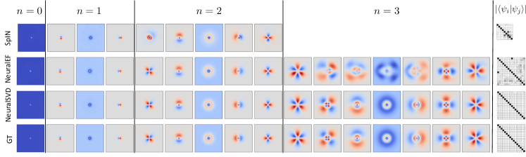
Figure 3: Visualization of the first 16 eigenfunctions of the 2D hydrogen atom. The first three rows present the learned eigenfunctions by SpIN (128), NeuralEF (512), and NeuralSVD${}_{\text{seq}}$ (512), respectively. Due to the memory complexity of SpIN, we ran SpIN with only 9 eigenstates. The learned functions are aligned by an orthogonal transformation via the orthogonal Procrustes method within each degenerate subspace to compare with the ground truth (GT) in the fourth row. The rightmost column visualizes the learned orthogonality.

Fig. 3 shows the learned eigenfunctions from SpIN (128), NeuralEF (512), and NeuralSVD${}_{\text{seq}}$ (512), where the numbers in the parentheses indicate used batch sizes. For comparison, we present the true eigenfunctions with a choice of canonical directions to plot the degenerate subspaces (last row). Note that SpIN and NeuralEF do not match the ground truths even after the rotation in several modes. Further, the learned functions (before rotation) are not orthogonal as visualized in the rightmost column. In contrast, NeuralSVD${}_{\text{seq}}$ can reliably match the correct eigenfunctions, with almost perfect orthogonality. Fig. 4 report several quantitative measures to evaluate the fidelity of learned eigenfunctions; see Sec. F.1.3 for the definitions of the measures. The results show that NeuralSVD${}_{\text{seq}}$ performs best, outperforming SpIN and NeuralEF by an order of magnitude.

Though NeuralSVD${}_{\text{jnt}}$ can recover the eigenfunctions reasonably well, it performs worse than NeuralSVD${}_{\text{seq}}$ as expected. We also note that while the computational and memory complexity of NeuralEF and NeuralSVD are almost the same, SpIN takes much longer time and consumes more memory due to the Cholesky decomposition and the need for storing the Jacobian; see Sec. B.2.1.

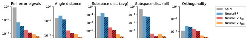
Figure 4: Summary of quantitative evaluations for solving TISE of 2D hydrogen atom. Non-hatched, light-colored bars represent batch size of 128, while hatched bars indicate batch size of 512. Reported measures are defined in Sec. F.1.3.

4.2 Data-Dependent Operators

Beyond analytical operators, we can also consider a special type of data-dependent kernels. Given a joint distribution $p(x,y)$, we consider

$$k(x,y)\mathrel{\mathop{\mathchar 58\relax missing}}=\frac{p(x,y)}{p(x)p(y)}-1$$

which is referred to as the canonical dependence kernel (CDK) [32, 33]. Although the CDK cannot be explicitly evaluated, it naturally defines the similarity between $x$ and $y$ based on their joint distribution, and thus can better capture the statistical relationship than a fixed, analytical kernel. Note that its induced integral kernel operator is the (centered) conditional expectation operator, i.e., $(\mathpzc{K}g)(x)=\operatorname{\mathsf{E}}_{p(y\mathchoice{\mspace{1.0mu}|\mspace{1.0mu}}{|}{|}{|}x)}[g(Y)]-\operatorname{\mathsf{E}}_{p(y)}[g(Y)]$ and $(\mathpzc{K}^{*}f)(y)=\operatorname{\mathsf{E}}_{p(x\mathchoice{\mspace{1.0mu}|\mspace{1.0mu}}{|}{|}{|}y)}[f(X)]-\operatorname{\mathsf{E}}_{p(x)}[f(X)]$, where $\mathpzc{K}^{*}$ denotes the adjoint of $\mathpzc{K}$. CDK appears and plays a central role in several statistics and machine learning applications, and various connections of CDK to the existing literature such as Hirschfeld–Gebelein–Rényi (HGR) maximal correlation [34, 35, 36] are discussed in Sec. B.

One special property of CDK is that we can compute the objective function using paired samples, even though we do not know the kernel value ${p(x,y)}/{(p(x)p(y))}$ in general. That is, the “operator term” $\langle g_{\ell}\mathchoice{\mspace{1.0mu}|\mspace{1.0mu}}{|}{|}{|}\mathpzc{K}f_{\ell}\rangle$ can be computed as

$$\langle g_{\ell}\mathchoice{\mspace{1.0mu}|\mspace{1.0mu}}{|}{|}{|}\mathpzc{K}f_{\ell}\rangle=\operatorname{\mathsf{E}}_{p(x,y)}[f_{\ell}(X)g_{\ell}(Y)]-\operatorname{\mathsf{E}}_{p(x)}[f_{\ell}(X)]\operatorname{\mathsf{E}}_{p(y)}[g_{\ell}(Y)],$$ (9)

where we change the measure $p(x)p(y)$ with $p(x,y)$ by the definition of $k(x,y)$.

Table 1: Evaluation of the ZS-SBIR task with the Sketchy Extended dataset [37, 38]. We note that the two baselines require ($\boldsymbol{\ast}$) a generative model, while NeuralSVD can learn representations directly without such.

Method	Ext. knowledge	Gen. model	Structured	P@100	mAP	Split
LCALE [39]	Word embeddings	$\boldsymbol{\ast}$	✗	0.583	0.476	1
IIAE [40]		$\boldsymbol{\ast}$	✗	0.659	0.573	1
NeuralSVD${}_{\text{jnt}}$			✓	${\bf 0.670}_{\pm 0.010}$	${\bf 0.581}_{\pm 0.008}$	1
				${\bf 0.724}_{\pm 0.008}$	${\bf 0.641}_{\pm 0.008}$	2

Application: Cross-Domain Retrieval.

One natural application of the CDK is in the cross-domain retrieval problem. Specifically, here we consider the zero-shot sketch-based image retrieval (ZS-SBIR) task proposed by Yelamarthi et al. [41]. The goal is to construct a good model that retrieves relevant photos $y_{i}$’s from a given query sketch $x$, only using a training set with no overlapping classes in the test set (hence zero-shot).

To apply the CDK framework, we define a natural joint distribution $p(x,y)$ for sketch $x$ and photo $y$, by picking a random pair of $(x,y)$ from the same class. Formally, the joint distribution is defined as $p(x,y)=\operatorname{\mathsf{E}}_{p(c)}[p(x\mathchoice{\mspace{1.0mu}|\mspace{1.0mu}}{|}{|}{|}c)p(y\mathchoice{\mspace{1.0mu}|\mspace{1.0mu}}{|}{|}{|}c)]$, where $p(c)$ denotes the class distribution, and $p(x\mathchoice{\mspace{1.0mu}|\mspace{1.0mu}}{|}{|}{|}c)$ and $p(y\mathchoice{\mspace{1.0mu}|\mspace{1.0mu}}{|}{|}{|}c)$ the class-conditional sketch and photo distributions, respectively. We emphasize that the resulting joint distribution is asymmetric, since $x$ and $y$ are two different modalities, and thus the existing frameworks, such as SpIN or NeuralEF, cannot be directly applied. We also note that the matrix approach, which is to compute the empirical CDK matrix and then perform SVD, is infeasible, as density ratio estimation for constructing the kernel matrix is nontrivial in the high-dimensional space. In sharp contrast, we can learn to decompose the CDK $k(x,y)=\frac{p(x,y)}{p(x)p(y)}\approx 1+{\bf f}(x)^{\intercal}{\bf g}(y)$ directly with NeuralSVD.

After learning the functions ${\bf f}$ and ${\bf g}$, for a given query $x$, we can retrieve based on the highest inner-product ${\bf f}(x)^{\intercal}{\bf g}(y)$ from $y\in\{y_{1},\ldots,y_{N}\}$. This approach has a natural probabilistic interpretation: “retrieve $y$, if $y$ is more likely to appear together than independently, i.e., $p(x,y)\gg p(x)p(y)$”. In addition to the interpretable retrieval scheme, the retrieval system can benefit from the learned spectral structure. That is, when successfully learned, most of the necessary information to reconstruct the CDK is concentrated in the first few dimensions, i.e., the most significant modes. We can thus potentially reduce the dimensionality of the learned embedding, essentially compressing it.

Experiment.

We aimed to learn $L=512$ singular functions, parameterizing them by a single network. We empirically found that NeuralSVD${}_{\text{seq}}$ performed much worse than NeuralSVD${}_{\text{jnt}}$ as discussed in the last paragraph in Sec. 3.2.1, only achieving Precision@100 around 0.2. Hence, we only report the result from NeuralSVD${}_{\text{jnt}}$. Since SpIN and NeuralEF are not directly applicable to asymmetric kernels, we do not include them in the comparison. We followed the standard training setup in the literature [40]. We report the Precision@100 (P@100) and mean average precision (mAP) scores on the two test splits in the literature; see Table 1. This shows that the CDK-based retrieval learned by NeuralSVD, albeit simple, can outperform the state-of-the-art representation learning methods based on generative models or with additional knowledge. Moreover, NeuralSVD learns structured representations, while the baselines only learn unstructured ones.

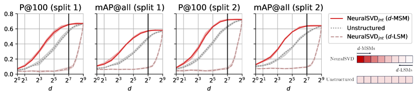
Figure 5: The P@100 and mAP performance of NeuralSVD on ZS-SBIR task, with varying dimensions $d$. NeuralSVD can achieve full performance only with one-quarter ($2^{7}=128$) of the full 512 dimensions, sweeping from the most significant modes.

As a demonstration of the structure in NeuralSVD representations, we verify that most information for retrieval is concentrated around the top modes. To illustrate this, we repeated and the following evaluation with 10 random initializations; see Fig. 5. First, from the NeuralSVD representations of $2^{9}=512$ dimensions, we used the $d$ most significant modes ($d$-MSMs) for $d\in\{1,2,2^{2},\ldots,2^{9}\}$, and evaluated the retrieval performance based on ${\bf f}_{[d]}(x)^{\intercal}{\bf g}_{[d]}(y)$. The performance rapidly grows as the dimensionality $d$ gets large, and the best is almost achieved at about $2^{7}=128$, which is only a quarter of the full dimension; see the red lines (NeuralSVD) and the vertical black lines.

As a further investigation, we consider two additional baselines. First, from the NeuralSVD representations, we evaluated the retrieval performance with the $d$ least significant modes ($d$-LSMs) for $d\in\{1,2,2^{2},\ldots,2^{9}\}$; see pink, dashed lines labeled with “NeuralSVD ($d$-LSM)”. The retrieval performance is very poor even when using the bottom 128 dimensions, which indicates that the LSMs do not encode much information. Second, we trained an unstructured embedding by training the same network with the LoRA objective without nesting, so that the network only learns the top-512 subspace of CDK; see gray, dotted lines labeled with “Unstructured”. As expected, its retrieval performance lies in the middle of NeuralSVD (MSM) and NeuralSVD (LSM). Hence, we can conclude that the learned representations with NeuralSVD are well-structured and effectively encode the information in a compact manner.

5 Concluding Remarks

In this paper, we proposed a new optimization framework called NeuralSVD that employs deep learning techniques to learn singular- (or eign-) functions of a linear operator. The core of the NeuralSVD framework is LoRA with the nesting technique, which we call NestedLoRA. In particular, our algorithm design results in a more efficient optimization process and a straightforward implementation owing to the unconstrained nature of the LoRA objective, without the explicit need for a computationally inefficient whitening procedure. The nesting techniques provide a consistency guarantee that the parametric singular functions will be learned correctly in the right order, in contrast to common regularization-based approaches, which do not often have such guarantees. We demonstrated its advantages against the existing methods in solving PDEs and also showed its potential in representation learning.

The parametric approach has empirically demonstrated its potential, for example, in quantum chemistry via neural network wavefunctions [20, 21], by showing much more favorable scalability than the classical methods. Our demonstration has also showcased the potential of the deep-learning-based framework, shedding light on its applicability to larger-scale problems. For example, we could potentially extend the applicability of the existing classical algorithms based on SVD/EVD in various fields, e.g., spectral embedding methods [6, 8], to large-scale, high-dimensional data, combined with the use of powerful neural networks. We discuss limitations and future directions in Appendix C.

Appendix A Reviews of Standard Linear Algebra Techniques

A.1 Empirical SVD and Nyström Method

A standard variational characterization of SVD is based on the following sequence of optimization problems:

$$\begin{aligned} \underset{\tilde{\phi}_{\ell}\in\mathcal{F},\tilde{\psi}_{\ell}\in\mathcal{G}}{\text{maximize~{}~{}}}&\langle\tilde{\psi}_{\ell}\mathchoice{\mspace{1.0mu}|\mspace{1.0mu}}{|}{|}{|}\mathpzc{T}\tilde{\phi}_{\ell}\rangle,\\ \text{subject~{}to~{}~{}}&\langle\tilde{\phi}_{i}\mathchoice{\mspace{1.0mu}|\mspace{1.0mu}}{|}{|}{|}\tilde{\phi}_{\ell}\rangle=\langle\tilde{\psi}_{i}\mathchoice{\mspace{1.0mu}|\mspace{1.0mu}}{|}{|}{|}\tilde{\psi}_{\ell}\rangle=\delta_{i\ell}\quad\forall i\in[\ell]\mathrel{\mathop{\mathchar 58\relax missing}}=\{1,\ldots,\ell\}.\end{aligned}$$ (10)

If $\mathpzc{T}$ is compact and the previous $(\ell-1)$ pairs of functions $\{(\tilde{\phi}_{i},\tilde{\psi}_{i})\}_{i\in[\ell-1]}$ are the top-$(\ell-1)$ singular functions, then the maximum value of the $\ell$-th problem, is attained by the $\ell$-th singular functions $(\phi_{\ell},\psi_{\ell})$ [42, Proposition A.2.8].

While the notion of SVD and its variational characterization are mathematically well defined, we cannot solve the infinite-dimensional problem (10) directly in general, except a very few cases with known closed-form solutions. Hence, in practice, a common approach is to perform the SVD of an empirical kernel matrix induced by finite points (samples, in learning scenarios). That is, given $x_{1},\ldots,x_{M}\sim p(x)$ and $y_{1},\ldots,y_{N}\sim p(y)$, we define the empirical kernel matrix $\hat{\mathsf{K}}\in\mathbb{R}^{M\times N}$ as $(\hat{\mathsf{K}})_{ij}\mathrel{\mathop{\mathchar 58\relax missing}}=k(x_{i},y_{j})$. Suppose we perform the (matrix) SVD of $\hat{\mathsf{K}}/\sqrt{MN}$ and obtain the top-$L$ left- and right-singular vectors $\hat{\mathsf{U}}=[\hat{{\bf u}}_{1},\ldots,\hat{{\bf u}}_{L}]\in\mathbb{R}^{M\times L}$ and $\hat{\mathsf{V}}=[\hat{{\bf v}}_{1},\ldots,\hat{{\bf v}}_{L}]\in\mathbb{R}^{N\times L}$ (normalized as $\hat{\mathsf{U}}^{\intercal}\hat{\mathsf{U}}=M\mathsf{I}$ and $\hat{\mathsf{V}}^{\intercal}\hat{\mathsf{V}}=N\mathsf{I}$, where $\mathsf{I}$ denotes the identity matrix) with the top-$L$ singular values $\hat{\sigma}_{1}\geq\ldots\geq\hat{\sigma}_{L}\geq 0$. Then, for each $\ell$, $\hat{{\bf u}}_{\ell}$ and $\hat{{\bf v}}_{\ell}$ approximate the evaluation of $\phi_{\ell}$ and $\psi_{\ell}$ at training data, i.e.,

$$\hat{{\bf u}}_{\ell}\approx[\phi_{\ell}(x_{1}),\ldots,\phi_{\ell}(x_{M})]^{\intercal},\quad\hat{{\bf v}}_{\ell}\approx[\psi_{\ell}(y_{1}),\ldots,\psi_{\ell}(y_{N})]^{\intercal},\quad\text{and}\quad\hat{\sigma}_{\ell}\approx\sigma_{\ell}.$$

Hence, for $\ell\geq 1$ with $\hat{\sigma}_{\ell}>0$, the $\ell$-th left-singular function at $x$ can be estimated as

$$\hat{\phi}_{\ell}(x)\mathrel{\mathop{\mathchar 58\relax missing}}=\frac{\hat{\sigma}_{\ell}^{-1}}{N}\sum_{j=1}^{N}k(x,y_{j})(\hat{{\bf v}}_{\ell})_{j},$$ (11)

which is a finite-sample approximation of the relation $\phi_{\ell}(x)={\sigma_{\ell}^{-1}}(K\psi_{\ell})(x)$. This is often referred to as the Nyström method; see, e.g., [23, 24].

Performing SVD of the kernel matrix $\mathsf{K}$ can be viewed as solving (10) with finite samples in the nonparametric limit. The sample SVD approach is limited, however, due to its memory and computational complexity. The time complexity of full SVD is $O(\min\{MN^{2},M^{2}N\})$ not scalable, but there exist iterative subspace methods that can perform top-$L$ SVD in an efficient way. Note, however, that the data matrix should be stored in memory to run standard SVD algorithms, which may not be feasible for large-scale data. Moreover, while the query complexity $O(N)$ or $O(M)$ of the Nyström method could be reduced by choosing a subset of training data, the challenge posed by the curse of dimensionality can potentially undermine the reliability of the Monte Carlo approximation (11) as an estimator.

A.2 On the Rayleigh–Ritz Method

The Rayleigh–Ritz method is a numerical algorithm to approximate eigenvalues [43]. The idea is to use an orthonormal basis of some smaller-dimensional subspace and solve the surrogate eigenvalue problem of smaller dimension projected on the subspace. The quality of the Rayleigh–Ritz approximation depends on the user-defined orthonormal basis $\{\mathchoice{\mspace{1.0mu}|\mspace{1.0mu}}{|}{|}{|}\phi_{j}\rangle\}_{j=1}^{d}$. That is, as the basis better captures the desired eigenmodes of the target operator, the approximation becomes more accurate. Otherwise, for example, if an eigenmode is orthogonal to the subspace of the eigenbasis, it cannot be found by this procedure. For completeness, we describe the procedure at the end of this section.

Given this standard tool, one may ask whether it is necessary to learn the ordered singular functions as done by NeuralSVD, SpIN, and NeuralEF. Instead, since NeuralSVD with LoRA (i.e., without nesting) can approximately learn the top-$L$ eigensubspace (Theorem 1), one can consider applying Rayleigh–Ritz with the learned functions from LoRA+NeuralSVD. Though the idea is valid and the full EVD of $L\times L$ matrix in Rayleigh–Ritz would be virtually at no cost, we remark that the two-stage procedure has several drawbacks compared to the direct approach with NeuralSVD. First, note that the learned functions with the LoRA objective are necessarily orthogonal and Gram–Schmidt process should be applied for obtaining the orthonormal basis before Rayleigh–Ritz. Note, however, that Gram–Schmidt becomes nontrivial in function spaces, as we need to compute the inner products and norms of functions at each step. Moreover, computing the inner products $\langle\phi_{i}\mathchoice{\mspace{1.0mu}|\mspace{1.0mu}}{|}{|}{|}\mathcal{T}\phi_{j}\rangle$ to compute the reduced operator as described below may introduce an additional estimation error.

More crucially, we empirically verified that NeuralSVD (either sequential or joint nesting) can attain lower subspace distance than LoRA+NeuralSVD, while being able to correctly ordered orthogonal eigenbasis simultaneously. Since the quality of Rayleigh–Ritz is limited by the quality of the given subspace, if the learned subspace has lower quality, the outcome must be worse. For example, in the 2D hydrogen atom experiment, we observed that the subspace distance over the 16 eigenmodes was $3.56\times 10^{-4}$${\pm 6.60\times 10^{-5}}$ with LoRA+NeuralSVD, while $2.12\times 10^{-4}$${\pm 2.09\times 10^{-5}}$ and $2.06\times 10^{-4}$${\pm 1.91\times 10^{-5}}$ were attained by JntNeuralSVD and SeqNeuralSVD, respectively; see Fig. 6(a). Since nesting does not increase complexity compared to the non-nested case via its efficient gradient implementation with masking, we argue that NeuralSVD can be more efficient than the two-stage approach.

Rayleigh–Ritz for Operator EVD.

For the ease of exposition, here we describe the procedure for an operator eigenvalue problem. Given a self-adjoint operator $\mathpzc{T}$, suppose that we wish to solve an eigenvalue problem

$$\mathpzc{T}\mathchoice{\mspace{1.0mu}|\mspace{1.0mu}}{|}{|}{|}\psi\rangle=\lambda\mathchoice{\mspace{1.0mu}|\mspace{1.0mu}}{|}{|}{|}\psi\rangle.$$

Since the problem may be hard to solve directly, the Rayleigh–Ritz method assumes that a set of orthonormal functions $\{\mathchoice{\mspace{1.0mu}|\mspace{1.0mu}}{|}{|}{|}\phi_{1}\rangle,\ldots,\mathchoice{\mspace{1.0mu}|\mspace{1.0mu}}{|}{|}{|}\phi_{d}\rangle\}$ for some $d\geq 1$, preferably $d\ll N$, and define $\mathsf{B}\in\mathbb{R}^{d\times d}$ such that $\mathsf{B}_{ij}\mathrel{\mathop{\mathchar 58\relax missing}}=\langle\phi_{i}\mathchoice{\mspace{1.0mu}|\mspace{1.0mu}}{|}{|}{|}\mathcal{T}\phi_{j}\rangle$. Then, we solve the eigenvalue problem

$$\mathsf{B}{\bf y}=\mu{\bf y}.$$

Given an eigenpair $(\mu_{i},{\bf y}_{i})$, we compute the Ritz function $\mathchoice{\mspace{1.0mu}|\mspace{1.0mu}}{|}{|}{|}\tilde{\psi}_{i}\rangle\mathrel{\mathop{\mathchar 58\relax missing}}=\sum_{j=1}^{d}y_{j}\mathchoice{\mspace{1.0mu}|\mspace{1.0mu}}{|}{|}{|}\phi_{j}\rangle$, and set the Ritz value $\tilde{\lambda}_{i}\mathrel{\mathop{\mathchar 58\relax missing}}=\mu_{i}$. The output of the Rayleigh–Ritz method are the Ritz pairs $\{(\tilde{\lambda}_{i},\tilde{\psi}_{i})\}_{i=1}^{d}$.

Appendix B Related Work

B.1 General Literature Review

B.1.1 Low-Rank Approximation

The theory of low-rank approximation was initially developed to solve partial differential equations (PDEs), including Schmidt [25]’s work; see, e.g., [44]. A special case for finite-dimensional matrices was independently discovered later by Eckart and Young [29] and Mirsky [45], which are perhaps better known in the literature. We refer an interested reader to [46] for detailed historical remarks. For matrices, Mirsky [45] extended the low-rank approximation theory to any unitarily invariant norms. While it would be interesting to extend the proposed framework in the current paper for other norms, they do not seem to easily admit an optimizable objective function.

B.1.2 Canonical Dependence Kernels

Interestingly, there exists a rich literature on decomposing canonical dependence kernels (CDK); see Sec. 4.2. The CDK has a close relationship to the Hirschfeld–Gebelein–Rényi (HGR) maximal correlation [34, 35, 36]. Note that the first singular functions are trivially constant functions, and the corresponding singular value $\sigma_{1}$ is always 1. When $L=2$, the second singular value is known as the HGR maximal correlation. In general, the optimization problem can be understood as the high-dimensional extension of the maximal correlation; for given $L\geq 2$, the optimal functions $\boldsymbol{\phi}^{\star}$ and $\boldsymbol{\psi}^{\star}$ are the optimal $L$-dimensional projections of $x\sim p(x)$ and $y\sim p(y)$ that are maximally correlated. The CDK plays an important role in learning applications and has been frequently redeveloped, bearing different names, e.g., correspondence analysis [47] and principal inertia components [48, 49] for finite alphabets, the contrastive kernel [50, 27] and the pointwise dependence [51] in the self-supervised representation learning setup.

The nonnested objective $\mathcal{L}_{\mathsf{LoRA}}({\bf f},{\bf g})$ for CDK was proposed and studied in Wang et al. [12] and related works, e.g., [52]. The H-score was first introduced by Wang et al. [12] who coined the term H-score (or Soft-HGR), for learning HGR maximal correlation functions with neural networks. It also appeared as a local approximation to log-loss of classification deep neural networks [52]. We mention in passing that the nonnested objective has been recently proposed independently under the name of the spectral contrastive loss [50], specifically when the CDK is induced by the random augmentation from the standard self-supervised representation learning setup. A recent work [53] proposes to learn features of two modalities based on the EVD of the so-called cross density ratio, which can be equivalently understood as the CDK of a symmetrized joint distribution. This paper, however, also only aims to characterize the top-$L$ subspace without the structure. Their optimization problem is based on minimizing the log-determinant of a normalized autocorrelation function; compared to our LoRA objective, the resulting optimization inherently suffers from biased gradients, which may lead to issues in practice.

B.1.3 Nesting

The idea of joint nesting was first introduced by Xu and Zheng [33] as a general construction to decompose multivariate dependence, which is equivalent to CDK in our terminology, for learning structured features; see the paper for more detailed discussion. The joint nesting proposed in this paper can be understood as an extension of the idea to general operators beyond CDK. While the idea of sequential nesting with LoRA is new, we observe that it conceptually resembles the idea of a class of streaming PCA algorithms such as [54, 28], in which the $(\ell+1)$-th eigenvector is updated under the assumption that the estimates for the first $\ell$ eigenvectors are accurate.

We note that a recent work [55] proposed learning a structured representation using a concept similar to the joint nesting technique introduced in our current paper. The method is referred to as Matryoshka Representation Learning (MRL). The key difference in MRL is that it assumes a labeled image dataset and uses the multi-class softmax cross-entropy loss function as its constituent loss function for “nesting”. Compared with MRL, the features learned by our CDK-based representation learning framework are interpretable as singular functions of the dependence kernel. This fundamental relation provides the learned features with theoretical guarantees, such as the uncorrelatedness of features. It is also worth noting that our features defined by the global minimizer of NestedLoRA_jnt is invariant to the choice of weights, while a different choice of such weights in MRL would characterize different features. Our framework is also not restricted to the supervised case, as demonstrated in the cross-domain retrieval example (Sec. 4.2).

B.1.4 Other Correlation Analysis Methods

There exists another line of related literature in correlation analysis. Deep canonical correlation analysis (DCCA) [56] can be understood as solving a restricted HGR maximal correlation problem, searching over a class of neural networks instead of all measurable functions. The DCCA objective function, however, requires a nontrivial optimization technique and cannot be easily extended to find higher modes. The correspondence-analysis neural network (CA-NN) [48] also aims to decompose the CDK based on a different optimization framework, but they involve the $L$-th Ky-Fan norm and the inversion of $L\times L$ matrix, which complicate the optimization procedure. Instead of deploying neural networks, Michaeli et al. [11] proposed to decompose an empirical CDK matrix constructed by the Gaussian kernel density estimators and coined the method as nonparametric canonical correspondence analysis (NCCA).

B.1.5 Neural-Network-Based Methods for Eigenvalue Problems

As alluded to earlier, there exists a rather separate line of work on solving eigenvalue problems using neural networks for solving linear PDEs that are in the form of an eigenvalue problem (EVP) in the physics or scientific computing community. Given the vastness of the literature and the rapid evolution of the field, providing a comprehensive overview is challenging. Nonetheless, we will emphasize key concepts and ideas.

Computational Physics Literature.

The idea of using neural networks for solving PDEs which can be reduced to eigenvalue problems dates back to [57], where an explicit Gram–Schmidt process was proposed to attain multiple eigenstates. Unlike the methods in the machine learning literature, many recent works rely on minimizing the sum of residual losses, mostly in the form of $\|(\mathpzc{T}-\lambda_{\ell}\mathpzc{I})\phi_{\ell}\|$ where $\lambda_{\ell}$ needs be also optimized or estimated from $\mathchoice{\mspace{1.0mu}|\mspace{1.0mu}}{|}{|}{|}\phi_{\ell}\rangle$, with regularization terms that penalize the normalization of and the orthogonality between the parametric functions; see [58, 59, 60, 61, 62, 63, 64, 65, 62, 66, 67, 68].

Other approaches include: Han et al. [69] proposes a stochastic differential equation framework that can learn the first mode of an eigenvalue problem; Yang et al. [70] propose a way to use neural networks for power and inverse power methods; Li and Ying [71] proposed a semigroup method for high dimensional elliptic PDEs and eigenvalue problems using neural networks. More broadly, there exist other deep-learning-based solvers for general PDEs beyond EVP PDEs such as deep Ritz method [72], deep Galerkin method [73], and Fourier neural operator [74].

Quantum Chemistry Literature.

Quantum chemistry has witnessed rapid recent advancements in this particular direction. While the main problem in quantum chemistry is to solve the TISE of a given electronic system, the problem size grows rapidly: the domain has $3N$ dimension with $N$ electrons, and thus the complexity of solving TISE exponentially blows up even with $N$ of a moderate size. Therefore, the development in this domain has been focused on developing a new neural network architecture (called neural network ansatzes) that better embed physical inductive bias for more expressivity. Representative works include [75], SchNet [76], Fermionic neural networks [77], FermiNet [21], PauliNet [20], and DeepErwin [78]; see a comprehensive, recent review paper [79] for the overview of the field.

In most, if not all, of the works, the quantum Monte Carlo (QMC), also known as variational Monte Carlo (VMC) [80], has been used as the de facto. QMC is essentially a special way to minimize the Rayleigh quotient to obtain the ground state energy. Until recently, most of the works focused on the ground state (i.e., the first bottom mode); a few recent exceptions are [81, 82], which proposed variations of QMC for excited states. We believe that applying the proposed NestedLoRA framework to quantum chemistry problem can be an exciting research direction.

B.2 Detailed Overview of SpIN and NeuralEF

Table 2: Comparison with SpIN [26] and NeuralEF [27].

	SpIN	NeuralEF	NeuralSVD
Goal	EVD	EVD	SVD/EVD
(a) To handle orthonormality constraints	Cholesky decomposition	function normalization	-
(b) To remove bias in gradient estimation	bi-level optimization; need to store Jacobian	large batch size	-

B.2.1 SpIN

Suppose that we wish to learn the top-$L$ eigenpairs of a linear operator $\mathpzc{T}$. For trial eigenfunctions $\hat{\phi}_{1},\ldots,\hat{\phi}_{L}$, define two $L\times L$ matrices $\Sigma$ and $\Pi$, which we call the gram matrix and the quadratic form matrix, respectively, as follows:

$$\Sigma_{\ell\ell^{\prime}}\mathrel{\mathop{\mathchar 58\relax missing}}=\langle\hat{\phi}_{\ell}\mathchoice{\mspace{1.0mu}|\mspace{1.0mu}}{|}{|}{|}\hat{\phi}_{\ell^{\prime}}\rangle\quad\text{and}\quad\Pi_{\ell\ell^{\prime}}\mathrel{\mathop{\mathchar 58\relax missing}}=\langle\hat{\phi}_{\ell}\mathchoice{\mspace{1.0mu}|\mspace{1.0mu}}{|}{|}{|}\mathpzc{T}\hat{\phi}_{\ell^{\prime}}\rangle.$$

Based on the trace maximization framework, we can solve the following optimization problem:

$$\operatorname*{maximize}_{\hat{\phi}_{1},\ldots,\hat{\phi}_{L}\in\mathcal{F}}\mathop{\rm tr}\nolimits(\Sigma^{-1}\Pi).$$

Let $\Sigma=\mathsf{L}\mathsf{L}^{\intercal}$ be the Cholesky decomposition of $\Sigma$, where $\mathsf{L}$ is a lower-triangular matrix. Define $\Lambda\mathrel{\mathop{\mathchar 58\relax missing}}=\mathsf{L}^{-1}\Pi\mathsf{L}^{-\intercal}\in\mathbb{R}^{L\times L}$. By the property of trace, we can write

$$\mathop{\rm tr}\nolimits(\Sigma^{-1}\Pi)=\mathop{\rm tr}\nolimits((\mathsf{L}\mathsf{L}^{\intercal})^{-1}\Pi) =\mathop{\rm tr}\nolimits(\mathsf{L}^{-1}\Pi\mathsf{L}^{-\intercal})=\mathop{\rm tr}\nolimits(\Lambda)=\sum_{\ell=1}^{L}\Lambda_{\ell\ell}.$$

Optimization with Masked Gradient.

The key idea behind the SpIN optimization framework is in the following lemma.

Lemma 5.

For each $\ell=1,\ldots,L$, $\Lambda_{\ell\ell}$ is only a function of $\hat{\phi}_{1},\ldots,\hat{\phi}_{\ell}$.

Proof.

It immediately follows from the upper triangular property of $\mathsf{L}^{-1}$. ∎

Assuming that $\hat{\phi}_{1},\ldots,\hat{\phi}_{\ell-1}$ learn the top-$(\ell-1)$ eigen-subspace, SpIN updates $\hat{\phi}_{\ell}$ to only maximize $\Lambda_{\ell\ell}$, i.e., based on the gradient $\mathop{}\!\partial_{\hat{\phi}_{\ell}}\Lambda_{\ell\ell}$ for each $\ell$. Once optimized, the learned functions can be orthogonalized by $\mathsf{L}^{-1}\hat{\boldsymbol{\phi}}$. Let $\mathsf{L}_{\Sigma}$ denote the Cholesky factor for a matrix $\Sigma$ and define

$$\mathsf{A}_{\Sigma,\Pi}\mathrel{\mathop{\mathchar 58\relax missing}}=\mathsf{L}_{\Sigma}^{-\intercal}\mathsf{triu}(\mathsf{L}_{\Sigma}^{-1}\Pi\mathsf{L}_{\Sigma}^{-\intercal}\mathop{\rm diag}\nolimits(\mathsf{L}_{\Sigma})^{-1}).$$

Then, the masked gradient can be collectively written as

$$-\tilde{\mathop{}\!\partial}_{\theta}\mathop{\rm tr}\nolimits(\Lambda) =-\operatorname{\mathsf{E}}_{p(x)}\Bigl{[}(\mathpzc{T}\hat{\boldsymbol{\phi}})(X)^{\intercal}\mathsf{L}_{\Sigma}^{-1}\mathop{\rm diag}\nolimits(\mathsf{L}_{\Sigma})^{-1}\frac{\mathop{}\!\partial\hat{\boldsymbol{\phi}}(X)}{\mathop{}\!\partial{\theta}}\Bigr{]}+\operatorname{\mathsf{E}}_{p(x)}\Bigl{[}\hat{\boldsymbol{\phi}}(X)^{\intercal}\mathsf{A}_{\Sigma,\Pi}\frac{\mathop{}\!\partial\hat{\boldsymbol{\phi}}(X)}{\mathop{}\!\partial{\theta}}\Bigr{]}.$$ (12)

See eq. (25) of [26] for the original expression with derivation. A naive estimator of this gradient with minibatch samples would be to plug in the empirical (unbiased) estimates of $\Sigma$ and $\Pi$, which are

$$\hat{\Sigma}\mathrel{\mathop{\mathchar 58\relax missing}}=\hat{\operatorname{\mathsf{E}}}_{p(x)}[\hat{\boldsymbol{\phi}}(X)\hat{\boldsymbol{\phi}}(X)^{\intercal}]\quad\text{and}\quad\hat{\Pi}\mathrel{\mathop{\mathchar 58\relax missing}}=\hat{\operatorname{\mathsf{E}}}_{p(x)}[\hat{\boldsymbol{\phi}}(X)(\mathpzc{T}\hat{\boldsymbol{\phi}})(X)^{\intercal}].$$

Note, however, the resulting gradient estimate is biased, since $\mathsf{L}_{\Sigma}$, $\mathsf{L}_{\Sigma}^{-1}$, and $\Sigma^{-1}$ are not linear in $\Sigma$.

Bi-level Stochastic Optimization for Unbiased Gradient Estimates.

To detour the issue with the biased gradient estimate, Pfau et al. [26] proposed to plug-in exponentially weighted moving average (EWMA) of two statistics into the expression, which can be understood as an instance of a bi-level stochastic optimization procedure with unbiased gradient estimates. To motivate the approach, we rewrite the second term of (12) as

$$\operatorname{\mathsf{E}}_{p(x)}\Bigl{[}\hat{\boldsymbol{\phi}}(X)^{\intercal}\mathsf{A}_{\Sigma,\Pi}\frac{\mathop{}\!\partial\hat{\boldsymbol{\phi}}(X)}{\mathop{}\!\partial{\theta}}\Bigr{]} =\mathop{\rm tr}\nolimits\Bigl{(}\mathsf{A}_{\Sigma,\Pi}\operatorname{\mathsf{E}}_{p(x)}\Bigl{[}\frac{\mathop{}\!\partial\hat{\boldsymbol{\phi}}(X)}{\mathop{}\!\partial{\theta}}\hat{\boldsymbol{\phi}}(X)^{\intercal}\Bigr{]}\Bigr{)}.$$

Based on the expression, we maintain the EWMAs of $\Sigma$ and $\operatorname{\mathsf{E}}_{p(x)}\Bigl{[}\frac{\mathop{}\!\partial\hat{\boldsymbol{\phi}}(X)}{\mathop{}\!\partial{\theta}}\hat{\boldsymbol{\phi}}(X)^{\intercal}\Bigr{]}$, which are denoted as $\bar{\Sigma}$ and $\bar{\mathbf{J}}$, and updated via minibatch samples as follows:

$$\bar{\Sigma} \leftarrow\beta\bar{\Sigma}+(1-\beta)\hat{\Sigma},$$ (13)

$$\bar{\mathbf{J}} \leftarrow\beta\bar{\mathbf{J}}+(1-\beta)\hat{\operatorname{\mathsf{E}}}_{p(x)}\Bigl{[}\frac{\mathop{}\!\partial\hat{\boldsymbol{\phi}}(X)}{\mathop{}\!\partial{\theta}}\hat{\boldsymbol{\phi}}(X)^{\intercal}\Bigr{]}.$$ (14)

Here $\beta\in[0,1]$ is the decay parameter for EWMA. Now, given these statistics, we update the parameter $\theta$ by the following gradient estimate with minibatch samples:

$$-\widehat{\tilde{\mathop{}\!\partial}}_{\theta}\mathop{\rm tr}\nolimits(\Lambda) =-\hat{\operatorname{\mathsf{E}}}_{p(x)}\Bigl{[}(\mathpzc{T}\hat{\boldsymbol{\phi}})(X)^{\intercal}\mathsf{L}_{\bar{\Sigma}}^{-1}\mathop{\rm diag}\nolimits(\mathsf{L}_{\bar{\Sigma}})^{-1}\frac{\mathop{}\!\partial\hat{\boldsymbol{\phi}}(X)}{\mathop{}\!\partial{\theta}}\Bigr{]}+\mathop{\rm tr}\nolimits(\mathsf{A}_{\bar{\Sigma},\hat{\Pi}}\bar{\mathbf{J}}).$$

Note that the randomness in the second term is in $\hat{\Pi}$ and the second term is linear in $\hat{\Pi}$. After all, the estimate is unbiased given $\bar{\Sigma}$ and $\bar{\mathbf{J}}$.

Discussion.

SpIN is a pioneering work, being the first parametric framework to perform the top-$L$ EVD of a self-adjoint operator with parametric eigenfunctions. However, the derivation of the masked gradient is rather involved, and the resulting algorithm’s complexity is not favorably scaling in $L$. In terms of the computational complexity, the Cholesky decomposition step that takes $O(L^{3})$ for each iteration is not scalable in $L$. Also, due to the bi-level stochastic optimization for unbiased gradient estimates, SpIN needs to maintain a separate copy of the Jacobian (14), which may consume significant memory with large networks. The decay parameter in the bi-level stochastic optimization is another sensitive hyperparameter to be tuned in the framework. Finally, we remark that the idea of masked gradient is similar to the sequential nesting, and thus when it is applied to a shared parameterization, it cannot guarantee a desired optimization behavior.

SpIN-X.

There exists a follow-up work of SpIN that proposed an alternative optimization method with several practical optimization techniques [31]. As the paper does not coin a term for the proposed method, we call it SpIN-X here. The proposed method is based on the following modified objective function

$$\mathcal{L}=\frac{1}{L}\Bigl{\{}-w_{0}\sum_{\ell=1}^{L}a_{\ell}\Lambda_{\ell\ell}+\sum_{\ell=1}^{L}w_{\ell}\|(\mathpzc{T}-\Lambda_{\ell\ell}\mathpzc{I})\hat{\phi}_{\ell}\|^{2}\Bigr{\}}.$$

Here, the weights $w_{0},\ldots,w_{L}$ are defined as $w_{\ell}\mathrel{\mathop{\mathchar 58\relax missing}}=(K_{0}+\ldots+K_{L})/K_{\ell}$, where $K_{\ell}\mathrel{\mathop{\mathchar 58\relax missing}}=\mathsf{sg}(\|\mathop{}\!\partial_{\theta}\mathcal{L}_{\ell}\|_{2})$, and $\Lambda_{\ell\ell}$ are eigenvalues still obtained from the Cholesky decomposition steps. Though the experimental results in [67] show improved results over SpIN, some optimization techniques such as balanced gradients are nontrivial to apply, and thus we do not include a comparison with this approach.

B.2.2 NeuralEF

In essence, NeuralEF [83] starts from the following characterization of eigenfunctions, which can be understood as a sequential version of (2).

Proposition 6.

Let $\mathpzc{T}\mathchoice{\colon}{\colon}{\mathchar 58\relax\mspace{1.0mu}}{\mathchar 58\relax}\mathcal{F}\to\mathcal{F}$ be a linear, self-adjoint operator, where $\mathcal{F}$ is a Hilbert space. Given functions $\tilde{\phi}_{1},\ldots,\tilde{\phi}_{\ell-1}\in\mathcal{F}$, consider the optimization problem

$$(P_{\ell})~{}~{}~{}\begin{aligned} \underset{\begin{subarray}{c}\tilde{\phi}_{\ell}\in\mathcal{F}\end{subarray}}{\text{maximize~{}~{}}}&\langle\tilde{\phi}_{\ell}\mathchoice{\mspace{1.0mu}|\mspace{1.0mu}}{|}{|}{|}\mathpzc{T}\tilde{\phi}_{\ell}\rangle\\ \text{subject~{}to~{}~{}}&\langle\tilde{\phi}_{\ell}\mathchoice{\mspace{1.0mu}|\mspace{1.0mu}}{|}{|}{|}\tilde{\phi}_{i}\rangle=\delta_{\ell i}\quad\forall 1\leq i\leq\ell.\end{aligned}$$

If $\tilde{\phi}_{1},\ldots,\tilde{\phi}_{\ell-1}$ are the top $\ell-1$ eigenfunctions of the operator $\mathpzc{T}$, then the solution $\tilde{\phi}_{\ell}$ of the optimization problem $(P_{\ell})$ is the $\ell$-th eigenfunction.

To avoid the explicit orthogonality constraint, NeuralEF proposes to solve the following optimization problem, generalizing the formulation of EigenGame [28] for operators:

$$(P_{\ell}^{\prime})~{}~{}~{}\begin{aligned} \underset{\begin{subarray}{c}\tilde{\phi}_{\ell}\in\mathcal{F}\end{subarray}}{\text{minimize~{}~{}}}&\mathcal{L}_{\ell}(\boldsymbol{\phi}_{1\mathchar 58\relax\ell})\mathrel{\mathop{\mathchar 58\relax missing}}=-\langle\tilde{\phi}_{\ell}\mathchoice{\mspace{1.0mu}|\mspace{1.0mu}}{|}{|}{|}\mathpzc{T}\tilde{\phi}_{\ell}\rangle+\sum_{i=1}^{\ell-1}\frac{\langle\tilde{\phi}_{\ell}\mathchoice{\mspace{1.0mu}|\mspace{1.0mu}}{|}{|}{|}\mathpzc{T}\tilde{\phi}_{i}\rangle}{\langle\tilde{\phi}_{i}\mathchoice{\mspace{1.0mu}|\mspace{1.0mu}}{|}{|}{|}\mathpzc{T}\tilde{\phi}_{i}\rangle}\\ \text{subject~{}to~{}~{}}&\langle\tilde{\phi}_{\ell}\mathchoice{\mspace{1.0mu}|\mspace{1.0mu}}{|}{|}{|}\tilde{\phi}_{\ell}\rangle=1.\end{aligned}$$ (15)

Replacing the constraints $\langle\tilde{\phi}_{\ell}\mathchoice{\mspace{1.0mu}|\mspace{1.0mu}}{|}{|}{|}\tilde{\phi}_{i}\rangle=0$ as $\langle\tilde{\phi}_{i}\mathchoice{\mspace{1.0mu}|\mspace{1.0mu}}{|}{|}{|}\mathpzc{T}\tilde{\phi}_{i}\rangle^{2}=0$ for each $1\leq i\leq\ell-1$, we can view $(P_{\ell}^{\prime})$ as a relaxed optimization problem of $(P_{\ell})$. Here, $\langle\tilde{\phi}_{i}\mathchoice{\mspace{1.0mu}|\mspace{1.0mu}}{|}{|}{|}\mathpzc{T}\tilde{\phi}_{i}\rangle^{-1}$ plays the role of a Lagrangian multiplier for the $i$-th constraint. With this specific choice of weights, this partially unconstrained optimization problem has the same guarantee (Proposition 6) for $(P_{\ell})$ as follows:

Theorem 7.

If $\tilde{\phi}_{1},\ldots,\tilde{\phi}_{\ell-1}$ are the top $\ell-1$ eigenfunctions $\phi_{1},\ldots,\phi_{\ell-1}$ of $\mathpzc{T}$, then the solution $\tilde{\phi}_{\ell}$ of the optimization problem $(P_{\ell}^{\prime})$ is the $\ell$-the eigenfunction.

Informal proof.

For the sake of simplicity, we assume that there are only $m$ finite eigenvalues $\lambda_{1},\ldots,\lambda_{m}$ and $\ell+1\leq m$. Let $\phi_{1},\phi_{2},\ldots$ be the eigenfunctions of $K$ which form an othornormal basis of $\mathcal{L}_{p(x)}^{2}(\mathcal{X})$. We first write a function $\tilde{\phi}_{\ell}$ as a linear combination of the eigenfunctions

$$\tilde{\phi}_{\ell}(x)=\sum_{i=1}^{\infty}\langle\tilde{\phi}_{\ell}\mathchoice{\mspace{1.0mu}|\mspace{1.0mu}}{|}{|}{|}\phi_{i}\rangle.$$

Then, we can readily observe that

$$\langle\tilde{\phi}_{\ell}\mathchoice{\mspace{1.0mu}|\mspace{1.0mu}}{|}{|}{|}\mathpzc{T}\tilde{\phi}_{\ell}\rangle =\sum_{i=1}^{m}\lambda_{i}\langle\tilde{\phi}_{\ell}\mathchoice{\mspace{1.0mu}|\mspace{1.0mu}}{|}{|}{|}\phi_{i}\rangle^{2},$$

$$\langle\tilde{\phi}_{\ell}\mathchoice{\mspace{1.0mu}|\mspace{1.0mu}}{|}{|}{|}\mathpzc{T}\phi_{i}\rangle =\lambda_{i}\langle\tilde{\phi}_{\ell}\mathchoice{\mspace{1.0mu}|\mspace{1.0mu}}{|}{|}{|}\phi_{i}\rangle,$$

$$\langle\phi_{i}\mathchoice{\mspace{1.0mu}|\mspace{1.0mu}}{|}{|}{|}\mathpzc{T}\phi_{i}\rangle =\lambda_{i}.$$

Therefore, the objective becomes

$$-\langle\tilde{\phi}_{\ell}\mathchoice{\mspace{1.0mu}|\mspace{1.0mu}}{|}{|}{|}\mathpzc{T}\tilde{\phi}_{\ell}\rangle+\sum_{i=1}^{\ell-1}\frac{\langle\tilde{\phi}_{\ell}\mathchoice{\mspace{1.0mu}|\mspace{1.0mu}}{|}{|}{|}\mathpzc{T}\phi_{i}\rangle^{2}}{\langle\phi_{i}\mathchoice{\mspace{1.0mu}|\mspace{1.0mu}}{|}{|}{|}\mathpzc{T}\phi_{i}\rangle} =-\sum_{i=1}^{m}\lambda_{i}\langle\tilde{\phi}_{\ell},\phi_{i}\rangle^{2}+\sum_{i=1}^{\ell-1}\lambda_{i}\langle\tilde{\phi}_{\ell},\phi_{i}\rangle^{2}$$

$$=-\sum_{i=\ell}^{m}\lambda_{i}\langle\tilde{\phi}_{\ell},\phi_{i}\rangle^{2},$$

which implies that the objective is uniquely minimized when $\langle\tilde{\phi}_{\ell},\phi_{i}\rangle=\delta_{i\ell}$ for $i\geq\ell$, i.e., when $\tilde{\phi}_{\ell}$ is the $\ell$-th eigenfunction $\phi_{\ell}$. ∎

Hence, solving the sequence of optimization problems $(P_{\ell}^{\prime})$ leads to finding the eigenfunctions in order. To emulate to solve the sequential optimization, Deng et al. [83] proposed to solve

$$\begin{aligned} \underset{\begin{subarray}{c}\tilde{\phi}_{1},\ldots,\tilde{\phi}_{L}\in\mathcal{F}\end{subarray}}{\text{minimize~{}~{}}}&\sum_{\ell=1}^{L}\Bigl{\{}-\langle\tilde{\phi}_{\ell}\mathchoice{\mspace{1.0mu}|\mspace{1.0mu}}{|}{|}{|}\mathpzc{T}\tilde{\phi}_{\ell}\rangle+\sum_{i=1}^{\ell-1}\frac{\langle\tilde{\phi}_{\ell}\mathchoice{\mspace{1.0mu}|\mspace{1.0mu}}{|}{|}{|}\mathpzc{T}\mathsf{sg}(\tilde{\phi}_{i})\rangle^{2}}{\langle\mathsf{sg}(\tilde{\phi}_{i})\mathchoice{\mspace{1.0mu}|\mspace{1.0mu}}{|}{|}{|}\mathpzc{T}\mathsf{sg}(\tilde{\phi}_{i})\rangle}\Bigr{\}}\\ \text{subject~{}to~{}~{}}&\langle\tilde{\phi}_{\ell}\mathchoice{\mspace{1.0mu}|\mspace{1.0mu}}{|}{|}{|}\tilde{\phi}_{\ell}\rangle=1\text{~{}for~{}}1\leq\ell\leq L.\end{aligned}$$

Here, $\mathsf{sg}$ denotes the stop-gradient operation, and thus this is not a properly defined optimization problem, rather defining an optimization procedure. It is worth emphasizing that the minimization procedure no longer guarantees a structured solution if the stop gradient operations are removed. To satisfy the normalization constraints, NeuralEF uses the $L_{2}$-batch normalization during training.

$$\mathop{}\!\partial_{\phi_{\ell}}\mathcal{L}_{\ell}(\boldsymbol{\phi}_{1\mathchar 58\relax\ell})=4\Bigl{\{}-\mathchoice{\mspace{1.0mu}|\mspace{1.0mu}}{|}{|}{|}\mathpzc{T}\phi_{\ell}\rangle+\sum_{i=1}^{\ell-1}\frac{\langle\phi_{i}\mathchoice{\mspace{1.0mu}|\mspace{1.0mu}}{|}{|}{|}\mathpzc{T}\phi_{\ell}\rangle}{\langle\phi_{i}\mathchoice{\mspace{1.0mu}|\mspace{1.0mu}}{|}{|}{|}\mathpzc{T}\phi_{i}\rangle}\mathchoice{\mspace{1.0mu}|\mspace{1.0mu}}{|}{|}{|}\mathpzc{T}\phi_{i}\rangle\Bigr{\}}.$$ (16)

Discussion.

NeuralEF improves SpIN in general, providing a simpler optimization procedure, i.e., without the costly Cholesky decomposition steps and the Jacobian updates. The game-theoretic formulation that stemmed from EigenGame [28] is similar to the idea of sequential nesting, and it might be problematic when applied to a shared parametrization as the sequential nesting is. The crucial difference of NeuralEF is that the $\ell$-th objective of NeuralEF has a guarantee only if the previous $(\ell-1)$ eigenfunctions are well learned, whereas the LoRA objective can characterize the eigensubspace and thus we can apply the joint nesting for a shared parameterization. Moreover, NestedLoRA can naturally handle SVD.

An Unbiased-Gradient Variation. We note that in the streaming PCA literature, the authors of EigenGame [28] proposed an unbiased variant of the original EigenGame in their subsequent work [84]. Following the same idea, one can easily think of an unbiased variant of NeuralEF, which corresponds to the following gradient:

$$\mathop{}\!\partial_{\phi_{\ell}}\mathcal{L}_{\ell}(\boldsymbol{\phi}_{1\mathchar 58\relax\ell})=4\Bigl{\{}-\mathchoice{\mspace{1.0mu}|\mspace{1.0mu}}{|}{|}{|}\mathpzc{T}\phi_{\ell}\rangle+\sum_{i=1}^{\ell-1}{\langle\phi_{i}\mathchoice{\mspace{1.0mu}|\mspace{1.0mu}}{|}{|}{|}\phi_{\ell}\rangle}\mathchoice{\mspace{1.0mu}|\mspace{1.0mu}}{|}{|}{|}\mathpzc{T}\phi_{i}\rangle\Bigr{\}}.$$

In our experiment, we used this variant instead of the original (16), as we found that the original NeuralEF performs much worse than its variant. In the current manuscript, we show that NeuralSVD can even outperform the improved version of NeuralEF.

Appendix C Limitations and Future Directions

The NeuralSVD framework we propose serves as a versatile template that empowers practitioners to select the most suitable parametric function and optimization details tailored to their specific problems. The main contribution of this paper is to provide an efficient optimization framework, NestedLoRA, in the parametric spectral decomposition approach, so that users can focus on choosing good architectures and optimization algorithms to meet the practical requirements of their specific problems.

In the following, we remark two considerations associated with the parametric approach in comparison to the nonparametric approach, which relies on standard numerical linear algebra techniques.

First, it is important to note that the parametric approach is theoretically less explored. The challenge lies in understanding the conditions under which a sufficiently large network can effectively approximate a given operator, as well as determining an optimization algorithm that guarantees convergence to the desired global optimizer within a specified optimization framework, such as NestedLoRA. Addressing this gap to provide performance guarantees represents a valuable avenue for further research.

Second, users engaging in the parametric approach are tasked with selecting an appropriate parametric function and optimization hyperparameters. Our present investigation has successfully showcased the efficacy of employing simple MLP architectures and specific hyperparameter choices in our illustrative examples. However, it is important to note that for more extensive applications, addressing the challenge of scalability common in modern deep learning methods may necessitate the adoption of more sophisticated architectural designs and fine-tuning in optimization algorithms. We thus advocate for future research to explore and design effective network architectures that are specifically tailored to individual operators and computation tasks, emphasizing the promising and important direction for further investigation.

Appendix D Technical Details and Deferred Proofs

D.1 Derivation of the Low-Rank Approximation Objective

Recall that we define the LoRA objective as

$$\mathcal{L}_{\mathsf{LoRA}}({\bf f}_{1\mathchar 58\relax L},{\bf g}_{1\mathchar 58\relax L}) \mathrel{\mathop{\mathchar 58\relax missing}}=-2\sum_{\ell=1}^{L}\langle g_{\ell}\mathchoice{\mspace{1.0mu}|\mspace{1.0mu}}{|}{|}{|}\mathpzc{T}f_{\ell}\rangle+\sum_{\ell=1}^{L}\sum_{\ell^{\prime}=1}^{L}\langle f_{\ell}\mathchoice{\mspace{1.0mu}|\mspace{1.0mu}}{|}{|}{|}f_{\ell^{\prime}}\rangle\langle g_{\ell}\mathchoice{\mspace{1.0mu}|\mspace{1.0mu}}{|}{|}{|}g_{\ell^{\prime}}\rangle.$$

When $\mathpzc{T}$ is a compact operator, the LoRA objective can be derived as the approximation error of $\mathpzc{T}$ via a low-rank expansion $\sum_{\ell=1}^{L}\mathchoice{\mspace{1.0mu}|\mspace{1.0mu}}{|}{|}{|}f_{\ell}\rangle\langle g_{\ell}\mathchoice{\mspace{1.0mu}|\mspace{1.0mu}}{|}{|}{|}$ measured in the squared Hilbert–Schmidt norm. For a linear operator $\mathpzc{T}\mathchoice{\colon}{\colon}{\mathchar 58\relax\mspace{1.0mu}}{\mathchar 58\relax}\mathcal{F}\to\mathcal{G}$ for Hilbert spaces $\mathcal{F}$ and $\mathcal{G}$, the Hilbert–Schmidt norm $\|\mathpzc{T}\|_{\mathsf{HS}}$ of an operator $\mathpzc{T}$ is defined as

$$\|\mathpzc{T}\|_{\mathsf{HS}}^{2}\mathrel{\mathop{\mathchar 58\relax missing}}=\sum_{i\in I}\|\mathpzc{T}\phi_{i}\|^{2}$$

for an orthonormal basis $\{\phi_{i}\mathchoice{\colon}{\colon}{\mathchar 58\relax\mspace{1.0mu}}{\mathchar 58\relax}i\in I\}$ of the Hilbert space $\mathcal{F}$. Note that the Hilbert–Schmidt norm is well-defined in that it is independent of the choice of the orthonormal basis. When $\mathcal{F}$ and $\mathcal{G}$ are finite-dimensional, i.e., when $\mathpzc{T}$ is a matrix, it boils down to the Frobenius norm. When $\|\mathpzc{T}\|_{\mathsf{HS}}<\infty$, $\mathpzc{T}$ is said to be compact.

Lemma 8.

If $\mathpzc{T}$ is compact, then

$$\mathcal{L}_{\mathsf{LoRA}}({\bf f}_{1\mathchar 58\relax L},{\bf g}_{1\mathchar 58\relax L}) =\Bigl{\|}\mathpzc{T}-\sum_{\ell=1}^{L}\mathchoice{\mspace{1.0mu}|\mspace{1.0mu}}{|}{|}{|}g_{\ell}\rangle\langle f_{\ell}\mathchoice{\mspace{1.0mu}|\mspace{1.0mu}}{|}{|}{|}\Bigr{\|}_{\mathsf{HS}}^{2}-\|\mathpzc{T}\|_{\mathsf{HS}}^{2}.$$ (17)

Proof.

Pick an orthonormal basis $\{\phi_{i}\mathchoice{\colon}{\colon}{\mathchar 58\relax\mspace{1.0mu}}{\mathchar 58\relax}i\in I\}$ of $\mathpzc{T}$. Note that $\sum_{i\in I}\mathchoice{\mspace{1.0mu}|\mspace{1.0mu}}{|}{|}{|}\phi_{i}\rangle\langle\phi_{i}\mathchoice{\mspace{1.0mu}|\mspace{1.0mu}}{|}{|}{|}=\mathpzc{I}$, where $\mathpzc{I}$ denotes the identity operator. Hence, we have

$$\Bigl{\|}\mathpzc{T}-\sum_{\ell=1}^{L}\mathchoice{\mspace{1.0mu}|\mspace{1.0mu}}{|}{|}{|}g_{\ell}\rangle\langle f_{\ell}\mathchoice{\mspace{1.0mu}|\mspace{1.0mu}}{|}{|}{|}\Bigr{\|}_{\mathsf{HS}}^{2}-\|\mathpzc{T}\|_{\mathsf{HS}}^{2} =\sum_{i\in I}\Bigl{\|}\mathpzc{T}\mathchoice{\mspace{1.0mu}|\mspace{1.0mu}}{|}{|}{|}\phi_{i}\rangle-\sum_{\ell=1}^{L}\mathchoice{\mspace{1.0mu}|\mspace{1.0mu}}{|}{|}{|}g_{\ell}\rangle\langle f_{\ell}\mathchoice{\mspace{1.0mu}|\mspace{1.0mu}}{|}{|}{|}\phi_{i}\rangle\Bigr{\|}^{2}-\sum_{i\in I}\|\mathpzc{T}\mathchoice{\mspace{1.0mu}|\mspace{1.0mu}}{|}{|}{|}\phi_{i}\rangle\|^{2}$$

$$=\sum_{i\in I}\Bigl{(}-2\sum_{\ell=1}^{L}\langle f_{\ell}\mathchoice{\mspace{1.0mu}|\mspace{1.0mu}}{|}{|}{|}\phi_{i}\rangle\langle g_{\ell}\mathchoice{\mspace{1.0mu}|\mspace{1.0mu}}{|}{|}{|}\mathcal{T}\mathchoice{\mspace{1.0mu}|\mspace{1.0mu}}{|}{|}{|}\phi_{i}\rangle+\sum_{\ell=1}^{L}\sum_{\ell^{\prime}=1}^{L}\langle f_{\ell}\mathchoice{\mspace{1.0mu}|\mspace{1.0mu}}{|}{|}{|}\phi_{i}\rangle\langle f_{\ell^{\prime}}\mathchoice{\mspace{1.0mu}|\mspace{1.0mu}}{|}{|}{|}\phi_{i}\rangle\langle g_{\ell}\mathchoice{\mspace{1.0mu}|\mspace{1.0mu}}{|}{|}{|}g_{\ell^{\prime}}\rangle\Bigr{)}$$

$$=-2\sum_{\ell=1}^{L}\Bigl{\langle}g_{\ell}\Big{\mathchoice{\mspace{1.0mu}|\mspace{1.0mu}}{|}{|}{|}missing}\mathcal{T}\Bigl{(}\sum_{i\in I}\mathchoice{\mspace{1.0mu}|\mspace{1.0mu}}{|}{|}{|}\phi_{i}\rangle\langle\phi_{i}\mathchoice{\mspace{1.0mu}|\mspace{1.0mu}}{|}{|}{|}\Bigr{)}\Bigr{\mathchoice{\mspace{1.0mu}|\mspace{1.0mu}}{|}{|}{|}missing}f_{\ell}\Bigr{\rangle}+\sum_{\ell=1}^{L}\sum_{\ell^{\prime}=1}^{L}\Bigl{\langle}f_{\ell}\Big{\mathchoice{\mspace{1.0mu}|\mspace{1.0mu}}{|}{|}{|}missing}\Bigl{(}\sum_{i\in I}\mathchoice{\mspace{1.0mu}|\mspace{1.0mu}}{|}{|}{|}\phi_{i}\rangle\langle\phi_{i}\mathchoice{\mspace{1.0mu}|\mspace{1.0mu}}{|}{|}{|}\Bigr{)}\Big{\mathchoice{\mspace{1.0mu}|\mspace{1.0mu}}{|}{|}{|}missing}f_{\ell^{\prime}}\Bigr{\rangle}\langle g_{\ell}\mathchoice{\mspace{1.0mu}|\mspace{1.0mu}}{|}{|}{|}g_{\ell^{\prime}}\rangle$$

$$=-2\sum_{\ell=1}^{L}\langle g_{\ell}\mathchoice{\mspace{1.0mu}|\mspace{1.0mu}}{|}{|}{|}\mathpzc{T}f_{\ell}\rangle+\sum_{\ell=1}^{L}\sum_{\ell^{\prime}=1}^{L}\langle f_{\ell}\mathchoice{\mspace{1.0mu}|\mspace{1.0mu}}{|}{|}{|}f_{\ell^{\prime}}\rangle\langle g_{\ell}\mathchoice{\mspace{1.0mu}|\mspace{1.0mu}}{|}{|}{|}g_{\ell^{\prime}}\rangle$$

$$=\mathcal{L}_{\mathsf{LoRA}}({\bf f}_{1\mathchar 58\relax L},{\bf g}_{1\mathchar 58\relax L}).\qed$$

Though this relationship (17) holds only for a compact operator, we remark that the LoRA objective (3) is well-defined for any operator $\mathpzc{T}$.

D.2 Proof of Theorem 1

From Lemma 8, Theorem 1 follows as a corollary of Schmidt’s LoRA theorem, stated below. ∎

Theorem 9 (Schmidt [25]).

Suppose that $\mathpzc{T}\mathchoice{\colon}{\colon}{\mathchar 58\relax\mspace{1.0mu}}{\mathchar 58\relax}\mathcal{F}\to\mathcal{G}$ is a compact operator with $\{(\sigma_{\ell},f_{\ell},g_{\ell})\}_{\ell=1}^{\infty}$ as its singular triplets. Define

$$({\bf f}^{\star},{\bf g}^{\star})\mathrel{\mathop{\mathchar 58\relax missing}}=\operatorname*{arg\,min}_{\begin{subarray}{c}f_{\ell}\in\mathcal{F},g_{\ell}\in\mathcal{G},\ \ell\in[L]\end{subarray}}\Bigl{\|}\mathpzc{T}-\sum_{\ell=1}^{L}\mathchoice{\mspace{1.0mu}|\mspace{1.0mu}}{|}{|}{|}g_{\ell}\rangle\langle f_{\ell}\mathchoice{\mspace{1.0mu}|\mspace{1.0mu}}{|}{|}{|}\Bigr{\|}_{\mathsf{HS}}^{2}.$$

If $\sigma_{L}>\sigma_{L+1}$, we have

$$\sum_{\ell=1}^{L}\mathchoice{\mspace{1.0mu}|\mspace{1.0mu}}{|}{|}{|}g_{\ell}^{\star}\rangle\langle f_{\ell}^{\star}\mathchoice{\mspace{1.0mu}|\mspace{1.0mu}}{|}{|}{|}=\sum_{\ell=1}^{L}\sigma_{\ell}\mathchoice{\mspace{1.0mu}|\mspace{1.0mu}}{|}{|}{|}\psi_{\ell}\rangle\langle\phi_{\ell}\mathchoice{\mspace{1.0mu}|\mspace{1.0mu}}{|}{|}{|}.$$

D.3 Proof of Theorem 2 (Sequential Nesting)

Recall that we assume

$$\sum_{i=1}^{\ell-1}\mathchoice{\mspace{1.0mu}|\mspace{1.0mu}}{|}{|}{|}g_{i}\rangle\langle f_{i}\mathchoice{\mspace{1.0mu}|\mspace{1.0mu}}{|}{|}{|}=\sum_{i=1}^{\ell-1}\sigma_{i}\mathchoice{\mspace{1.0mu}|\mspace{1.0mu}}{|}{|}{|}\psi_{i}\rangle\langle\phi_{i}\mathchoice{\mspace{1.0mu}|\mspace{1.0mu}}{|}{|}{|}.$$

By Lemma 8, the LoRA objective can be written as

$$\mathcal{L}_{\mathsf{LoRA}}({\bf f}_{1\mathchar 58\relax\ell},{\bf g}_{1\mathchar 58\relax\ell}) =\Bigl{\|}\mathpzc{T}-\sum_{i=1}^{\ell}\mathchoice{\mspace{1.0mu}|\mspace{1.0mu}}{|}{|}{|}g_{i}\rangle\langle f_{i}\mathchoice{\mspace{1.0mu}|\mspace{1.0mu}}{|}{|}{|}\Bigr{\|}_{\mathsf{HS}}^{2}-\|\mathpzc{T}\|_{\mathsf{HS}}^{2}$$

$$=\Bigl{\|}\sum_{i\geq 1}\sigma_{i}\mathchoice{\mspace{1.0mu}|\mspace{1.0mu}}{|}{|}{|}\psi_{i}\rangle\langle\phi_{i}\mathchoice{\mspace{1.0mu}|\mspace{1.0mu}}{|}{|}{|}-\sum_{i=1}^{\ell-1}\sigma_{i}\mathchoice{\mspace{1.0mu}|\mspace{1.0mu}}{|}{|}{|}\psi_{i}\rangle\langle\phi_{i}\mathchoice{\mspace{1.0mu}|\mspace{1.0mu}}{|}{|}{|}-\mathchoice{\mspace{1.0mu}|\mspace{1.0mu}}{|}{|}{|}g_{\ell}\rangle\langle f_{\ell}\mathchoice{\mspace{1.0mu}|\mspace{1.0mu}}{|}{|}{|}\Bigr{\|}_{\mathsf{HS}}^{2}-\|\mathpzc{T}\|_{\mathsf{HS}}^{2}$$

$$=\Bigl{\|}\sum_{i\geq\ell}\sigma_{i}\mathchoice{\mspace{1.0mu}|\mspace{1.0mu}}{|}{|}{|}\psi_{i}\rangle\langle\phi_{i}\mathchoice{\mspace{1.0mu}|\mspace{1.0mu}}{|}{|}{|}-\mathchoice{\mspace{1.0mu}|\mspace{1.0mu}}{|}{|}{|}g_{\ell}\rangle\langle f_{\ell}\mathchoice{\mspace{1.0mu}|\mspace{1.0mu}}{|}{|}{|}\Bigr{\|}_{\mathsf{HS}}^{2}-\|\mathpzc{T}\|_{\mathsf{HS}}^{2}.$$

Hence, minimizing $\mathcal{L}_{\mathsf{LoRA}}({\bf f}_{1\mathchar 58\relax\ell},{\bf g}_{1\mathchar 58\relax\ell})$ with respect to $(f_{\ell},g_{\ell})$ is equivalent to minimizing the LoRA objective $\mathcal{L}_{\mathsf{LoRA}}(f_{\ell},g_{\ell};\mathcal{T}_{\geq\ell})$ defined with respect to the truncated operator $\mathcal{T}_{\geq\ell}\mathrel{\mathop{\mathchar 58\relax missing}}=\sum_{i\geq\ell}\sigma_{i}\mathchoice{\mspace{1.0mu}|\mspace{1.0mu}}{|}{|}{|}\psi_{i}\rangle\langle\phi_{i}\mathchoice{\mspace{1.0mu}|\mspace{1.0mu}}{|}{|}{|}$. Since $\sigma_{\ell}>\sigma_{\ell+1}$, by Schmidt’s theorem (Theorem 9), the global optimizer must satisfy $\mathchoice{\mspace{1.0mu}|\mspace{1.0mu}}{|}{|}{|}g_{\ell}\rangle\langle f_{\ell}\mathchoice{\mspace{1.0mu}|\mspace{1.0mu}}{|}{|}{|}=\sigma_{\ell}\mathchoice{\mspace{1.0mu}|\mspace{1.0mu}}{|}{|}{|}\psi_{\ell}\rangle\langle\phi_{\ell}\mathchoice{\mspace{1.0mu}|\mspace{1.0mu}}{|}{|}{|}$. ∎

D.4 Proof of Theorem 3 (Joint Nesting)

We first prove the following lemma; Theorem 3 readily follows as a corollary.

Lemma 10.

Suppose that all the nonzero singular values of the target kernel are distinct. If $\sigma_{\ell}>\sigma_{\ell+1}$, the objective function $\tilde{\mathcal{L}}({\bf f},{\bf g})\mathrel{\mathop{\mathchar 58\relax missing}}=\mathcal{L}_{\mathsf{LoRA}}({\bf f}_{1\mathchar 58\relax\ell},{\bf g}_{1\mathchar 58\relax\ell})+w\mathcal{L}_{\mathsf{LoRA}}({\bf f}_{[L]},{\bf g}_{[L]})$ with $w>0$ is minimized if and only if

$$\sum_{i=1}^{\ell}\mathchoice{\mspace{1.0mu}|\mspace{1.0mu}}{|}{|}{|}g_{i}^{*}\rangle\langle f_{i}^{*}\mathchoice{\mspace{1.0mu}|\mspace{1.0mu}}{|}{|}{|} =\sum_{i=1}^{\ell}\sigma_{i}\mathchoice{\mspace{1.0mu}|\mspace{1.0mu}}{|}{|}{|}\psi_{i}\rangle\langle\phi_{i}\mathchoice{\mspace{1.0mu}|\mspace{1.0mu}}{|}{|}{|}\quad\text{ and }\quad\sum_{i=\ell+1}^{L}\mathchoice{\mspace{1.0mu}|\mspace{1.0mu}}{|}{|}{|}g_{i}^{*}\rangle\langle f_{i}^{*}\mathchoice{\mspace{1.0mu}|\mspace{1.0mu}}{|}{|}{|}=\sum_{i=\ell+1}^{L}\sigma_{i}\mathchoice{\mspace{1.0mu}|\mspace{1.0mu}}{|}{|}{|}\psi_{i}\rangle\langle\phi_{i}\mathchoice{\mspace{1.0mu}|\mspace{1.0mu}}{|}{|}{|}.$$

Proof.

First, note that by the Schmidt theorem (Theorem 9),

$$\mathcal{L}_{\mathsf{LoRA}}({\bf f}_{1\mathchar 58\relax\ell},{\bf g}_{1\mathchar 58\relax\ell})\geq\mathcal{L}_{\mathsf{LoRA}}({\bf f}_{1\mathchar 58\relax\ell}^{*},{\bf g}_{1\mathchar 58\relax\ell}^{*})=\sum_{i=1}^{\ell}\sigma_{\ell}^{2},$$

where the equality holds if and only if

$$\sum_{i=1}^{\ell}\mathchoice{\mspace{1.0mu}|\mspace{1.0mu}}{|}{|}{|}g_{i}^{*}\rangle\langle f_{i}^{*}\mathchoice{\mspace{1.0mu}|\mspace{1.0mu}}{|}{|}{|}=\sum_{i=1}^{\ell}\sigma_{i}\mathchoice{\mspace{1.0mu}|\mspace{1.0mu}}{|}{|}{|}\psi_{i}\rangle\langle\phi_{i}\mathchoice{\mspace{1.0mu}|\mspace{1.0mu}}{|}{|}{|}.$$

Using this property, we immediately have a lower bound

$$\mathcal{L}_{\mathsf{LoRA}}({\bf f}_{1\mathchar 58\relax\ell},{\bf g}_{1\mathchar 58\relax\ell})+w\mathcal{L}_{\mathsf{LoRA}}({\bf f}_{1\mathchar 58\relax L},{\bf g}_{1\mathchar 58\relax L})\geq\sum_{i=1}^{\ell}\sigma_{i}^{2}+w\sum_{j=1}^{L}\sigma_{j}^{2},$$

where the equality holds if and only if

$$\sum_{i=1}^{\ell}\mathchoice{\mspace{1.0mu}|\mspace{1.0mu}}{|}{|}{|}g_{i}^{*}\rangle\langle f_{i}^{*}\mathchoice{\mspace{1.0mu}|\mspace{1.0mu}}{|}{|}{|} =\sum_{i=1}^{\ell}\sigma_{i}\mathchoice{\mspace{1.0mu}|\mspace{1.0mu}}{|}{|}{|}\psi_{i}\rangle\langle\phi_{i}\mathchoice{\mspace{1.0mu}|\mspace{1.0mu}}{|}{|}{|}\quad\text{ and }\quad\sum_{i=1}^{L}\mathchoice{\mspace{1.0mu}|\mspace{1.0mu}}{|}{|}{|}g_{i}^{*}\rangle\langle f_{i}^{*}\mathchoice{\mspace{1.0mu}|\mspace{1.0mu}}{|}{|}{|}=\sum_{i=1}^{L}\sigma_{i}\mathchoice{\mspace{1.0mu}|\mspace{1.0mu}}{|}{|}{|}\psi_{i}\rangle\langle\phi_{i}\mathchoice{\mspace{1.0mu}|\mspace{1.0mu}}{|}{|}{|},$$

which is equivalent to

$$\sum_{i=1}^{\ell}\mathchoice{\mspace{1.0mu}|\mspace{1.0mu}}{|}{|}{|}g_{i}^{*}\rangle\langle f_{i}^{*}\mathchoice{\mspace{1.0mu}|\mspace{1.0mu}}{|}{|}{|}=\sum_{i=1}^{\ell}\sigma_{i}\mathchoice{\mspace{1.0mu}|\mspace{1.0mu}}{|}{|}{|}\psi_{i}\rangle\langle\phi_{i}\mathchoice{\mspace{1.0mu}|\mspace{1.0mu}}{|}{|}{|}\quad\text{ and }\quad\sum_{i=\ell+1}^{L}\mathchoice{\mspace{1.0mu}|\mspace{1.0mu}}{|}{|}{|}g_{i}^{*}\rangle\langle f_{i}^{*}\mathchoice{\mspace{1.0mu}|\mspace{1.0mu}}{|}{|}{|} =\sum_{i=\ell+1}^{L}\sigma_{i}\mathchoice{\mspace{1.0mu}|\mspace{1.0mu}}{|}{|}{|}\psi_{i}\rangle\langle\phi_{i}\mathchoice{\mspace{1.0mu}|\mspace{1.0mu}}{|}{|}{|}.\qed$$

We are now ready to prove Theorem 3.

Proof of Theorem 3.

By inductively applying Lemma 10 to the grouping $\mathcal{L}_{\mathsf{jnt}}({\bf f},{\bf g})=\sum_{i=1}^{\ell}w_{i}\mathcal{L}_{\mathsf{LoRA}}({\bf f}_{[i]},{\bf g}_{[i]})+\sum_{i=\ell+1}^{L}w_{i}\mathcal{L}_{\mathsf{LoRA}}({\bf f}_{[i]},{\bf g}_{[i]})$ for $\ell=1,\ldots,L-1$, a minimizer must satisfy

$$\sum_{i=1}^{\ell}\mathchoice{\mspace{1.0mu}|\mspace{1.0mu}}{|}{|}{|}g_{i}^{*}\rangle\langle f_{i}^{*}\mathchoice{\mspace{1.0mu}|\mspace{1.0mu}}{|}{|}{|}=\sum_{i=1}^{\ell}\sigma_{i}\mathchoice{\mspace{1.0mu}|\mspace{1.0mu}}{|}{|}{|}\psi_{i}\rangle\langle\phi_{i}\mathchoice{\mspace{1.0mu}|\mspace{1.0mu}}{|}{|}{|},$$

for each $\ell=1,\ldots,L$. This implies that the equivalence $\mathchoice{\mspace{1.0mu}|\mspace{1.0mu}}{|}{|}{|}g_{i}^{*}\rangle\langle f_{i}^{*}\mathchoice{\mspace{1.0mu}|\mspace{1.0mu}}{|}{|}{|}=\sigma_{i}\mathchoice{\mspace{1.0mu}|\mspace{1.0mu}}{|}{|}{|}\psi_{i}\rangle\langle\phi_{i}\mathchoice{\mspace{1.0mu}|\mspace{1.0mu}}{|}{|}{|}$ should hold term by term. ∎

D.5 One-Shot Computation of Jointly Nested Objective

The gradient of the joint nesting objective (8) can be computed based on the following observation:

Proposition 11 (One-shot computation).

Given a positive weight vector $\boldsymbol{\mathsf{w}}$, define $\boldsymbol{\mathsf{m}}\in\mathbb{R}^{L}$ and ${\mathsf{M}}\in\mathbb{R}^{L\times L}$ as $\mathsf{m}_{i}\mathrel{\mathop{\mathchar 58\relax missing}}=\sum_{\ell=i}^{L}w_{\ell}$ and ${\mathsf{M}}_{ij}\mathrel{\mathop{\mathchar 58\relax missing}}=\mathsf{m}_{\max\{i,j\}}$. Then, the nested objective is written as

$$\mathcal{L}_{\mathsf{jnt}}({\bf f},{\bf g};\boldsymbol{\mathsf{w}}) \mathrel{\mathop{\mathchar 58\relax missing}}=-2\sum_{\ell=1}^{L}\mathsf{m}_{\ell}\langle g_{\ell}\mathchoice{\mspace{1.0mu}|\mspace{1.0mu}}{|}{|}{|}\mathpzc{T}f_{\ell}\rangle+\sum_{\ell=1}^{L}\sum_{\ell^{\prime}=1}^{L}{\mathsf{M}}_{\ell\ell^{\prime}}\langle f_{\ell}\mathchoice{\mspace{1.0mu}|\mspace{1.0mu}}{|}{|}{|}f_{\ell^{\prime}}\rangle\langle g_{\ell}\mathchoice{\mspace{1.0mu}|\mspace{1.0mu}}{|}{|}{|}g_{\ell^{\prime}}\rangle.$$

Proof.

Recall that

$$\mathcal{L}_{\mathsf{jnt}}({\bf f},{\bf g};\boldsymbol{\mathsf{w}}) =\sum_{\ell=1}^{L}w_{\ell}\mathcal{L}_{\mathsf{LoRA}}({\bf f}_{1\mathchar 58\relax\ell},{\bf g}_{1\mathchar 58\relax\ell})$$

$$=\sum_{\ell=1}^{L}w_{\ell}\Bigl{\{}-2\sum_{i=1}^{\ell}\langle g_{i}\mathchoice{\mspace{1.0mu}|\mspace{1.0mu}}{|}{|}{|}\mathpzc{T}f_{i}\rangle+\sum_{i=1}^{\ell}\sum_{j=1}^{\ell}\langle f_{i}\mathchoice{\mspace{1.0mu}|\mspace{1.0mu}}{|}{|}{|}f_{j}\rangle\langle g_{i}\mathchoice{\mspace{1.0mu}|\mspace{1.0mu}}{|}{|}{|}g_{j}\rangle\Bigr{\}}$$

For the first term, we can write

$$\sum_{\ell=1}^{L}w_{\ell}\sum_{i=1}^{\ell}\langle g_{i}\mathchoice{\mspace{1.0mu}|\mspace{1.0mu}}{|}{|}{|}\mathpzc{T}f_{i}\rangle =\sum_{\ell=1}^{L}w_{\ell}\sum_{i=1}^{\ell}f_{i}(x)g_{i}(y)=\sum_{\ell=1}^{L}\mathsf{m}_{\ell}\langle g_{\ell}\mathchoice{\mspace{1.0mu}|\mspace{1.0mu}}{|}{|}{|}\mathpzc{T}f_{\ell}\rangle,$$

where $\mathsf{m}_{\ell}\mathrel{\mathop{\mathchar 58\relax missing}}=\sum_{i=\ell}^{L}w_{i}$. For the second term, we can write

$$\sum_{\ell=1}^{L}w_{\ell}\sum_{1\leq i,j\leq\ell}\langle f_{i}\mathchoice{\mspace{1.0mu}|\mspace{1.0mu}}{|}{|}{|}f_{j}\rangle\langle g_{i}\mathchoice{\mspace{1.0mu}|\mspace{1.0mu}}{|}{|}{|}g_{j}\rangle =\sum_{1\leq i,j\leq L}{\mathsf{M}}_{ij}\langle f_{i}\mathchoice{\mspace{1.0mu}|\mspace{1.0mu}}{|}{|}{|}f_{j}\rangle\langle g_{i}\mathchoice{\mspace{1.0mu}|\mspace{1.0mu}}{|}{|}{|}g_{j}\rangle,$$

where ${\mathsf{M}}_{ij}\mathrel{\mathop{\mathchar 58\relax missing}}=\mathsf{m}_{\max\{i,j\}}=\sum_{\ell=\max\{i,j\}}^{L}w_{\ell}$. This concludes the proof. ∎

D.6 EVD with Non-Compact Operators

For a self-adjoint operator $\mathpzc{T}$, we can apply our framework by considering the induced LoRA objective

$$\mathcal{L}_{\mathsf{LoRA}}({\bf f}_{1\mathchar 58\relax L})\mathrel{\mathop{\mathchar 58\relax missing}}=-2\sum_{\ell=1}^{L}\langle f_{\ell}\mathchoice{\mspace{1.0mu}|\mspace{1.0mu}}{|}{|}{|}\mathpzc{T}f_{\ell}\rangle+\sum_{\ell=1}^{L}\sum_{\ell^{\prime}=1}^{L}\langle f_{\ell}\mathchoice{\mspace{1.0mu}|\mspace{1.0mu}}{|}{|}{|}f_{\ell^{\prime}}\rangle^{2}.$$

Though the original LoRA theorem of Schmidt (Theorem 9) holds for a compact operator, it can be extended to a certain class of non-compact operators, which have discrete eigenvalues.

Theorem 12.

For a self-adjoint operator $\mathpzc{T}$, define

$${\bf f}^{\star}\mathrel{\mathop{\mathchar 58\relax missing}}=\operatorname*{arg\,min}_{\begin{subarray}{c}f_{\ell}\in\mathcal{F},\ \ell\in[L]\end{subarray}}\mathcal{L}_{\mathsf{LoRA}}({\bf f}).$$

Suppose that the operator $\mathpzc{T}$ has $r$ positive eigenvalues $\lambda_{1}\geq\ldots\geq\lambda_{r}>0\geq\lambda_{r+1}\geq\ldots$ with corresponding orthonormal eigenfunctions $\{\phi_{\ell}\}_{\ell\geq 1}$, for some $r\in\mathbb{N}\cup\{\infty\}$. If $r<\infty$, the span of $\mathchoice{\mspace{1.0mu}|\mspace{1.0mu}}{|}{|}{|}{\bf f}^{\star}\rangle$ is equal to the span of the top-$\min\{L,r\}$ eigenfunctions of the operator $\mathpzc{T}$, or more precisely

$$\sum_{\ell=1}^{L}\mathchoice{\mspace{1.0mu}|\mspace{1.0mu}}{|}{|}{|}f_{\ell}^{\star}\rangle\langle f_{\ell}^{\star}\mathchoice{\mspace{1.0mu}|\mspace{1.0mu}}{|}{|}{|}=\sum_{\ell=1}^{\min\{L,r\}}\lambda_{\ell}\mathchoice{\mspace{1.0mu}|\mspace{1.0mu}}{|}{|}{|}\phi_{\ell}\rangle\langle\phi_{\ell}\mathchoice{\mspace{1.0mu}|\mspace{1.0mu}}{|}{|}{|}.$$

If $r=\infty$, i.e., when there are countably infinitely many positive eigenvalues, the same holds if $\lambda_{L}>\lambda_{L+1}$.

As a consequence of this theorem, when we optimize the $\mathchoice{\mspace{1.0mu}|\mspace{1.0mu}}{|}{|}{|}{\bf f}_{1\mathchar 58\relax L}\rangle$ with nesting for $L>r$, one can easily show that the optimal $\mathchoice{\mspace{1.0mu}|\mspace{1.0mu}}{|}{|}{|}f_{r+1}^{\star}\rangle,\ldots,\mathchoice{\mspace{1.0mu}|\mspace{1.0mu}}{|}{|}{|}f_{L}^{\star}\rangle$ are zero functions; we omit the proof.

Proof.

We first consider when $r$ is finite. Define the positive part of the operator as

$$\mathpzc{T}_{+}\mathrel{\mathop{\mathchar 58\relax missing}}=\sum_{\ell=1}^{r}\lambda_{\ell}\mathchoice{\mspace{1.0mu}|\mspace{1.0mu}}{|}{|}{|}\phi_{\ell}\rangle\langle\phi_{\ell}\mathchoice{\mspace{1.0mu}|\mspace{1.0mu}}{|}{|}{|},$$

which is compact by definition. Then, $\mathpzc{T}_{+}-\mathpzc{T}$ is PSD with eigenvalues $0\leq-\lambda_{r+1}\leq-\lambda_{r+2}\leq\ldots$ and eigenfunctions $\{\phi_{\ell}\}_{\ell\geq r+1}$. Then, we can rewrite and lower bound the LoRA objective as

$$\mathcal{L}_{\mathsf{LoRA}}({\bf f}_{1\mathchar 58\relax L}) =\Bigl{\|}\mathpzc{T}_{+}-\sum_{\ell=1}^{L}\mathchoice{\mspace{1.0mu}|\mspace{1.0mu}}{|}{|}{|}f_{\ell}\rangle\langle f_{\ell}\mathchoice{\mspace{1.0mu}|\mspace{1.0mu}}{|}{|}{|}\Bigr{\|}_{\mathsf{HS}}^{2}-\|\mathpzc{T}_{+}\|_{\mathsf{HS}}^{2}+2\sum_{\ell=1}^{L}\langle f_{\ell}\mathchoice{\mspace{1.0mu}|\mspace{1.0mu}}{|}{|}{|}(\mathpzc{T}_{+}-\mathpzc{T})f_{\ell}\rangle$$

$$\stackrel{{\scriptstyle\mathchoice{\hbox to0.0pt{\hss$\displaystyle{(a)}$\hss}}{\hbox to0.0pt{\hss$\textstyle{(a)}$\hss}}{\hbox to0.0pt{\hss$\scriptstyle{(a)}$\hss}}{\hbox to0.0pt{\hss$\scriptscriptstyle{(a)}$\hss}}}}{{\geq}}\Bigl{\|}\mathpzc{T}_{+}-\sum_{\ell=1}^{L}\mathchoice{\mspace{1.0mu}|\mspace{1.0mu}}{|}{|}{|}f_{\ell}\rangle\langle f_{\ell}\mathchoice{\mspace{1.0mu}|\mspace{1.0mu}}{|}{|}{|}\Bigr{\|}_{\mathsf{HS}}^{2}-\|\mathpzc{T}_{+}\|_{\mathsf{HS}}^{2},$$

where the inequality $(a)$ follows since $\mathpzc{T}_{+}-\mathpzc{T}$ is PSD. We note that the lower bound is minimized if and only if the span of $\mathchoice{\mspace{1.0mu}|\mspace{1.0mu}}{|}{|}{|}{\bf f}^{\star}\rangle$ is equal to the span of the top-$\min\{L,r\}$ eigenfunctions of the operator $\mathpzc{T}_{+}$ by applying Schmidt’s theorem (Theorem 9). We further note that $(a)$ holds with equality, as $\mathchoice{\mspace{1.0mu}|\mspace{1.0mu}}{|}{|}{|}f_{1}^{\star}\rangle,\ldots,\mathchoice{\mspace{1.0mu}|\mspace{1.0mu}}{|}{|}{|}f_{L}^{\star}\rangle$ belong to the null space of $\mathpzc{T}_{+}-\mathpzc{T}$. Hence, this concludes that the LoRA objective is minimized if and only if the span of $\mathchoice{\mspace{1.0mu}|\mspace{1.0mu}}{|}{|}{|}{\bf f}^{\star}\rangle$ is equal to the span of the top-$\min\{L,r\}$ eigenfunctions of the operator $\mathpzc{T}$.

When $r=\infty$, given that $\lambda_{L}>\lambda_{L+1}$, the rank-$L$ approximation of $\mathpzc{T}$

$$\mathpzc{T}_{L}\mathrel{\mathop{\mathchar 58\relax missing}}=\sum_{\ell=1}^{L}\lambda_{\ell}\mathchoice{\mspace{1.0mu}|\mspace{1.0mu}}{|}{|}{|}\phi_{\ell}\rangle\langle\phi_{\ell}\mathchoice{\mspace{1.0mu}|\mspace{1.0mu}}{|}{|}{|}$$

is well-defined. The same proof for $r<\infty$ is valid if we replace $\mathpzc{T}_{+}$ with $\mathpzc{T}_{L}$. ∎

Appendix E Implementation Details with Code Snippets

In this section, we explain how to implement the proposed NestedLoRA updates, providing readily deployable code snippets written in PyTorch. These code snippets are simplified from the actual implementation which can be found online for the ease of exposition.

E.1 Helper Functions: Computing Nesting Masks and Metric Loss

As noted in Sec. 3.2.2, both versions of NestedLoRA can be implemented in a unified way via the nesting masks $(\mathsf{m}_{\ell})_{\ell\in[L]}$ and $({\mathsf{M}}_{i\ell})_{i\in[L],\ell\in[L]}$. Recall that for joint nesting, given positive weights $(w_{1},\ldots,w_{L})$, we define $\mathsf{m}_{\ell}\mathrel{\mathop{\mathchar 58\relax missing}}=\sum_{i=\ell}^{L}w_{i}$ and ${\mathsf{M}}_{i\ell}\mathrel{\mathop{\mathchar 58\relax missing}}=\mathsf{m}_{\max\{i,\ell\}}$.

⬇

1def get_joint_nesting_masks(weights: np.ndarray, set_first_mode_const: bool = False):

2 vector_mask = list(np.cumsum(list(weights)[::-1])[::-1])

3 if set_first_mode_const:

4 vector_mask = [vector_mask[0]] + vector_mask

5 vector_mask = torch.tensor(np.array(vector_mask)).float()

6 matrix_mask = torch.minimum(vector_mask.unsqueeze(1), vector_mask.unsqueeze(1).T).float()

7 return vector_mask, matrix_mask

Here, when the argument set_first_mode_const is set to be True, it outputs masks for CDK, for which we explicitly add the constant first mode; see Sec. E.4.

The sequential nesting (4) can be implemented by defining $\mathsf{m}_{\ell}\mathrel{\mathop{\mathchar 58\relax missing}}=1$ and ${\mathsf{M}}_{i\ell}\mathrel{\mathop{\mathchar 58\relax missing}}=\mathds{1}\{i\leq\ell\}$.

⬇

1def get_sequential_nesting_masks(L, set_first_mode_const: bool = False):

2 if set_first_mode_const:

3 L += 1

4 vector_mask = torch.ones(L)

5 matrix_mask = torch.triu(torch.ones(L, L))

6 return vector_mask, matrix_mask

In the LoRA objective (3), the second term (with nesting), which we call the metric loss,

$$\sum_{\ell=1}^{L}\sum_{\ell^{\prime}=1}^{L}{\mathsf{M}}_{\ell\ell^{\prime}}\langle f_{\ell}\mathchoice{\mspace{1.0mu}|\mspace{1.0mu}}{|}{|}{|}f_{\ell^{\prime}}\rangle\langle g_{\ell}\mathchoice{\mspace{1.0mu}|\mspace{1.0mu}}{|}{|}{|}g_{\ell^{\prime}}\rangle=\sum_{\ell=1}^{L}\sum_{\ell^{\prime}=1}^{L}({\mathsf{M}}\odot\Lambda_{{\bf f}}\odot\Lambda_{{\bf g}})_{\ell\ell^{\prime}}$$ (18)

is independent of the operator, where we define $(\Lambda_{{\bf f}})_{\ell\ell^{\prime}}\mathrel{\mathop{\mathchar 58\relax missing}}=\langle f_{\ell}\mathchoice{\mspace{1.0mu}|\mspace{1.0mu}}{|}{|}{|}f_{\ell^{\prime}}\rangle$ for $\ell,\ell^{\prime}\in[L]$ and $\odot$ denotes the elementwise matrix product. Given samples $x_{1},\ldots,x_{B}$, we can estimate each entry of the matrix $\Lambda_{\bf f}\in\mathbb{R}^{L\times L}$ by

$$(\hat{\Lambda}_{{\bf f}})_{\ell\ell^{\prime}}\mathrel{\mathop{\mathchar 58\relax missing}}=\frac{1}{B}\sum_{b=1}^{B}f_{\ell}(x)f_{\ell^{\prime}}(x),$$

which can be computed with PyTorch as:

⬇

1def compute_lambda(f):

2 return torch.einsum(’bl,bm->lm’, f, f) / f.shape[0] # (L, L)

Then, the metric loss can be computed as follows:

⬇

1def compute_loss_metric(f, g, matrix_mask):

2 lam_f = compute_lambda(f)

3 lam_g = compute_lambda(g)

4 # compute loss_metric = E_{p(x)p(y)}[(f^T(x) g(y))^2]

5 # f: (B1, L)

6 # g: (B2, L)

7 # lam_f, lam_g: (L, L)

8 return (matrix_mask * lam_f * lam_g).sum(), lam_f, lam_g # O(L ** 2)

Note that this metric loss needs not be computed when computing gradients.

E.2 NestedLoRA Gradient Computation for Analytical Operators

In this section, we explain how to implement the NestedLoRA gradient updates for analytical operators. For the sake of simplicity, we explain for the implementation for EVD; the implementation for SVD can be found in our official PyTorch implementation.

For EVD of a self-adjoint operator $\mathcal{T}$, identifying ${\bf g}$ with ${\bf f}$, we need to compute the gradient

$$(\mathop{}\!\partial_{f_{\ell}}\mathcal{L})(x_{b})=2\Bigl{\{}-\mathsf{m}_{\ell}(\mathpzc{T}f_{\ell})(x_{b})+\sum_{i=1}^{L}{\mathsf{M}}_{i\ell}f_{i}(x_{b})\langle f_{i}\mathchoice{\mspace{1.0mu}|\mspace{1.0mu}}{|}{|}{|}f_{\ell}\rangle\Bigr{\}}$$ (19)

for each $\ell\in[L]$; see (8) for the general expression. We can compute the gradient in an unbiased manner by plugging in the unbiased estimate of $\Lambda_{{\bf f}}$ based on $\{x_{1}^{\prime},\ldots,x_{B^{\prime}}^{\prime}\}$. We remark that the minibatch samples for estimating $\Lambda_{{\bf f}}$ needs to be independent to $\{x_{1},\ldots,x_{B}\}$ so that the overall gradient estimate for $\langle\mathop{}\!\partial_{\theta}f_{\ell}\mathchoice{\mspace{1.0mu}|\mspace{1.0mu}}{|}{|}{|}\mathop{}\!\partial_{f_{\ell}}\mathcal{L}\rangle$ becomes unbiased. This can be efficiently implemented in a vectorized manner by writing a custom backward function with the automatic differentiation package of PyTorch as follows. In what follows, we assume that $\{{\bf f}(x_{b})\}_{b=1}^{B}$ and $\{(\mathcal{T}{\bf f})(x_{b})\}_{b=1}^{B}$ are already computed for a given ${\bf f}$ and provided as f and Tf, resepectively. Further, f1 and f2 must be independent to each other.

⬇

1class NestedLoRALossFunctionEVD(torch.autograd.Function):

2 @staticmethod

3 @torch.cuda.amp.custom_fwd

4 def forward(

5 ctx: torch.autograd.function.FunctionCtx,

6 f,

7 Tf,

8 f1,

9 f2,

10 vector_mask,

11 matrix_mask,

12 ):

13 """

14 the reduction assumed here is ‘mean‘ (i.e., we take average over batch)

15 f: (B, L) or (B, L, O)

16 Tf: (B, L) or (B, L, O)

17 f1: (B1, L) or (B1, L, O)

18 f2: (B2, L) or (B2, L, O)

19 warning: f1 and f2 must be independent

20 """

21 ctx.vector_mask = vector_mask = vector_mask.to(f.device)

22 ctx.matrix_mask = matrix_mask = matrix_mask.to(f.device)

23 loss_metric, lam_f1, lam_f2 = compute_loss_metric(f1, f2, matrix_mask)

24 ctx.save_for_backward(f, Tf, f1, f2, lam_f1, lam_f2)

25 # compute loss_operator = -2 * E_{p(x)}[\sum_{l=1}^L f_l^T(x) (Tf_l)(x)]

26 loss_operator = - 2 * torch.einsum(’l,bl,bl->b’, vector_mask, f, Tf).mean() # O(B1 * L * O)

27 loss = loss_operator + loss_metric

28 return loss

29

30 @staticmethod

31 @torch.cuda.amp.custom_bwd

32 def backward(

33 ctx: torch.autograd.function.FunctionCtx,

34 grad_output: torch.Tensor

35 ) -> Tuple[torch.Tensor, ...]:

36 """

37 Args:

38 ctx: The context object to retrieve saved tensors

39 grad_output: The gradient of the loss with respect to the output

40 """

41 f, Tf, f1, f2, lam_f1, lam_f2 = ctx.saved_tensors

42 operator_f = - (4 / f.shape[0]) * torch.einsum(’l,bl->bl’, ctx.vector_mask, Tf)

43 metric_f1 = (2 / f1.shape[0]) * torch.einsum(’lm,lm,bl->bm’, ctx.matrix_mask, lam_f2, f1)

44 metric_f2 = (2 / f2.shape[0]) * torch.einsum(’lm,lm,bl->bm’, ctx.matrix_mask, lam_f1, f2)

45 return grad_output * operator_f, None, grad_output * metric_f1, grad_output * metric_f2, None, None, None

In practice, when given a minibatch $\{x_{1},\ldots,x_{B}\}$, we can use the entire batch to compute f and Tf, and split f into two equal parts and plug in them to f1 and f2 to ensure the independence. In what follows, the operator is given as an abstract function operator, whose interface is explained in the next section (Sec. E.3).

⬇

1def compute_loss_operator(

2 model,

3 operator,

4 x,

5 importance=None,

6):

7 Tf, f = operator(model, x, importance=importance)

8 f1, f2 = torch.chunk(f, 2)

9 loss = NestedLoRALossFunctionEVD.apply(

10 f, Tf, f1, f2,

11 vector_mask,

12 matrix_mask,

13 )

14 return loss, dict(f=f, Tf=Tf, eigvals=None)

After this function returns loss, calling loss.backward() will backpropagate the gradients based on the custom backward function, and populate the gradient for each model parameter.

E.3 Importance Sampling

Unlike machine learning applications where the sampling distribution is given by data, the underlying measure $\mu(x)$ is the Lebesgue measure over a given domain when solving PDEs. Note that, when the domain is not bounded, we cannot sample from the measure, and thus it is necessary to introduce a sampling distribution to apply our framework. Given a distribution $p_{\mathsf{tr}}(x)$ that is supported over the support of $\mu(x)$, the inner product between $\mathchoice{\mspace{1.0mu}|\mspace{1.0mu}}{|}{|}{|}f\rangle$ and $\mathchoice{\mspace{1.0mu}|\mspace{1.0mu}}{|}{|}{|}\mathpzc{T}f\rangle$ can be written as

$$\langle f\mathchoice{\mspace{1.0mu}|\mspace{1.0mu}}{|}{|}{|}\mathpzc{T}f\rangle =\int f(x)\mathpzc{T}f(x)\mu(x)\mathop{}\!\mathrm{d}x$$

$$=\int f(x)\sqrt{\frac{\mu(x)}{p_{\mathsf{tr}}(x)}}\mathpzc{T}f(x)\sqrt{\frac{\mu(x)}{p_{\mathsf{tr}}(x)}}p_{\mathsf{tr}}(x)\mathop{}\!\mathrm{d}x$$

$$=\int\frac{f(x)}{\sqrt{w_{\mathsf{tr}}(x)}}\frac{\mathpzc{T}f(x)}{\sqrt{w_{\mathsf{tr}}(x)}}p_{\mathsf{tr}}(x)\mathop{}\!\mathrm{d}x.$$

Here, we define the (training) importance function $w_{\mathsf{tr}}(x)\mathrel{\mathop{\mathchar 58\relax missing}}=\frac{p_{\mathsf{tr}}(x)}{\mu(x)}$. For the case of the Lebesgue measure, one can simply regard $\mu(x)$ as 1. It is sometimes crucial to choose a good training sampling distribution, especially for high-dimensional problems.

Suppose now that we directly parameterize $\frac{f(x)}{\sqrt{w_{\mathsf{tr}}(x)}}$ by a neural network $\tilde{f}(x)$. Then, the inner product can be computed as

$$\langle f\mathchoice{\mspace{1.0mu}|\mspace{1.0mu}}{|}{|}{|}\mathpzc{T}f\rangle=\int\tilde{f}(x)\frac{\mathpzc{T}f(x)}{\sqrt{w_{\mathsf{tr}}(x)}}p_{\mathsf{tr}}(x)\mathop{}\!\mathrm{d}x.$$

Here, $\mathpzc{T}f(x)$ can be computed by applying the operator $\mathpzc{T}$ to the function $x\mapsto\sqrt{w_{\mathsf{tr}}(x)}\tilde{f}(x)$.

During the test phase, we may use another test distribution $p_{\mathsf{te}}(x)$ to evaluate the inner product. Given another valid sampling distribution $p_{\mathsf{te}}(x)$,

$$\langle f\mathchoice{\mspace{1.0mu}|\mspace{1.0mu}}{|}{|}{|}\mathpzc{T}f\rangle=\int\tilde{f}(x)\frac{\mathpzc{T}f(x)}{\sqrt{w_{\mathsf{tr}}(x)}}\frac{p_{\mathsf{tr}}(x)}{p_{\mathsf{te}}(x)}p_{\mathsf{te}}(x)\mathop{}\!\mathrm{d}x=\int\tilde{f}(x)\frac{\mathpzc{T}f(x)}{\sqrt{w_{\mathsf{tr}}(x)}}\frac{w_{\mathsf{tr}}(x)}{w_{\mathsf{te}}(x)}p_{\mathsf{te}}(x)\mathop{}\!\mathrm{d}x,$$

where we define the (test) importance function $w_{\mathsf{te}}(x)\mathrel{\mathop{\mathchar 58\relax missing}}=\frac{p_{\mathsf{te}}(x)}{\mu(x)}$. Again, for high-dimensional problems, it is crucial to choose a good sampling distribution for reliable evaluation.

In our implementation, the operator is defined with the following interface: given a neural network model $\tilde{f}(x)$ and a training importance function $p_{\mathsf{te}}(x)$, operator(model, x, importance) outputs $\frac{\mathpzc{T}f(x)}{\sqrt{w_{\mathsf{tr}}(x)}}$ and $\tilde{f}(x)$, so that they can be taken to the inner product directly under $p_{\mathsf{tr}}(x)$. Given this, the original function value $f(x)$ can be recovered as $f(x)=\sqrt{w_{\mathsf{tr}}(x)}\tilde{f}(x)$.

For example, we implement the negative Hamiltonian as follows:

⬇

1class NegativeHamiltonian:

2 def __init__(self,

3 local_potential_ftn,

4 scale_kinetic=1.,

5 laplacian_eps=1e-5,

6 n_particles=1):

7 self.laplacian_eps = laplacian_eps

8 self.laplacian = VectorizedLaplacian(eps=laplacian_eps)

9 self.local_potential_ftn = local_potential_ftn

10 self.scale_kinetic = scale_kinetic

11 self.n_particles = n_particles

12

13 def __call__(self, f, xs, importance=None, threshold=1e5):

14 # threshold is to detect an anomaly in the hamiltonian

15 lap, grad, fs = self.laplacian(f, xs, importance)

16 kinetic = - self.scale_kinetic * lap

17 potential = self.local_potential_ftn(xs.reshape((xs.shape[0], self.n_particles, -1))).view(-1, 1) * fs

18 hamiltonian = kinetic + potential

19 return - hamiltonian, fs

Here, VectorizedLaplacian refers to a function for vectorized Laplacian computation, whose implementation can be found in our code.

E.4 NestedLoRA Gradient Computation for CDK

Recall that the CDK is defined as $k(x,y)=\overline{k}(x,y)-1$ with $\overline{k}(x,y)\mathrel{\mathop{\mathchar 58\relax missing}}=\frac{p(x,y)}{p(x)p(y)}$. We note that it is known that $\overline{k}(x,y)$ has the constant functions as the singular functions with singular value 1, i.e., $(1,x\mapsto 1,y\mapsto 1)$ is the first singular triplet of $\overline{k}(x,y)$; see, e.g., [32]. Hence, the term “$-1$” in the definition of CDK is to remove the first trivial mode of $\overline{k}(x,y)$.

In our implementation, we handle the decomposition of CDK by considering $\overline{k}(x,y)$ with explicitly augmenting the constant functions as the fictitious first singular functions, so that we effectively learn from the second singular functions of $\overline{k}(x,y)$ and on. For $\overline{k}(x,y)=\frac{p(x,y)}{p(x)p(y)}$, the “operator term” $\langle g_{\ell}\mathchoice{\mspace{1.0mu}|\mspace{1.0mu}}{|}{|}{|}\overline{\mathpzc{K}}f_{\ell}\rangle$ can be computed as, again by change of measure,

$$\langle g_{\ell}\mathchoice{\mspace{1.0mu}|\mspace{1.0mu}}{|}{|}{|}\overline{\mathpzc{K}}f_{\ell}\rangle=\operatorname{\mathsf{E}}_{p(x,y)}[f_{\ell}(X)g_{\ell}(Y)].$$

Hence, compared to (19), the gradient becomes, for each $\ell=1,\ldots,L$,

$$(\mathop{}\!\partial_{f_{\ell}}\mathcal{L})(x_{b})=2\Bigl{\{}-\mathsf{m}_{\ell}g_{\ell}(x_{b})+\sum_{i=0}^{L}{\mathsf{M}}_{i\ell}f_{i}(x_{b})\langle g_{i}\mathchoice{\mspace{1.0mu}|\mspace{1.0mu}}{|}{|}{|}g_{\ell}\rangle\Bigr{\}}$$ (20)

where we set $f_{0}(x)\equiv 1$ and $g_{0}(y)\equiv 1$; $(\mathop{}\!\partial_{g_{\ell}}\mathcal{L})(x_{b})$ is similarly computed. The following snippet implements this gradient using a custom gradient as before. Note that the constant 1’s are explicitly appended as the first mode in line 16-18.

⬇

1class NestedLoRALossFunctionForCDK(torch.autograd.Function):

2 @staticmethod

3 @torch.cuda.amp.custom_fwd

4 def forward(

5 ctx: torch.autograd.function.FunctionCtx,

6 f,

7 g,

8 vector_mask,

9 matrix_mask,

10 ):

11 """

12 the reduction assumed here is ‘mean‘ (i.e., we take average over batch)

13 f: (B, L)

14 g: (B, L)

15 """

16 pad = nn.ConstantPad1d((1, 0), 1)

17 f = pad(f)

18 g = pad(g)

19 ctx.vector_mask = vector_mask = vector_mask.to(f.device)

20 ctx.matrix_mask = matrix_mask = matrix_mask.to(f.device)

21 loss_metric, lam_f, lam_g = compute_loss_metric(f, g, matrix_mask)

22 ctx.save_for_backward(f, g, lam_f, lam_g)

23 # compute loss_operator = -2 * E_{p(x,y)}[f^T(x) g(y)]

24 loss_operator = - 2 * torch.einsum(’l,bl,bl->b’, vector_mask, f, g).mean() # O(B1 * L)

25 loss = loss_operator + loss_metric

26 gram_matrix = f @ g.T # (B, B); each entry is (f^T(x_i) g(y_j))

27 rs_joint = gram_matrix.diag()

28 rs_indep = off_diagonal(gram_matrix)

29 return loss, loss_operator, loss_metric, rs_joint, rs_indep

30

31 @staticmethod

32 @torch.cuda.amp.custom_bwd

33 def backward(

34 ctx: torch.autograd.function.FunctionCtx,

35 grad_output: torch.Tensor,

36 *args

37 ) -> Tuple[torch.Tensor, ...]:

38 """

39 Args:

40 ctx: The context object to retrieve saved tensors

41 grad_output: The gradient of the loss with respect to the output

42 """

43 f, g, lam_f, lam_g = ctx.saved_tensors

44 # for grad(f)

45 operator_f = - (2 / f.shape[0]) * torch.einsum(’l,bl->bl’, ctx.vector_mask, g)

46 metric_f = (2 / f.shape[0]) * torch.einsum(’il,il,bi->bl’, ctx.matrix_mask, lam_g, f)

47 grad_f = operator_f + metric_f

48 # for grad(g)

49 operator_g = - (2 / g.shape[0]) * torch.einsum(’l,bl->bl’, ctx.vector_mask, f)

50 metric_g = (2 / g.shape[0]) * torch.einsum(’il,il,bi->bl’, ctx.matrix_mask, lam_f, g)

51 grad_g = operator_g + metric_g

52 grad_f = grad_f[:, 1:]

53 grad_g = grad_g[:, 1:]

54 return grad_output * grad_f, grad_output * grad_g, None, None, None, None

In practice, given minibatch samples $\{(x_{b},y_{b})\}_{b=1}^{B}$ drawn from a joint distribution $p(x,y)$, we can compute $\{({\bf f}(x_{b}),{\bf g}(y_{b}))\}_{b=1}^{B}$ and plug in to the function above as follows.

⬇

1def compute_loss(

2 f,

3 g,

4) -> torch.Tensor:

5 return NestedLoRALossFunctionForCDK.apply(

6 f,

7 g,

8 vector_mask,

9 matrix_mask,

10 )

Here, vector_mask and matrix_mask should be computed using the mask computing functions in Sec. E.1 with set_first_mode_const=True.

E.5 Spectrum Estimation via Norm Estimation

As alluded to in the main text, we can estimate the singular values $(\sigma_{1},\ldots,\sigma_{L})$ from the learned functions and training data, i.e.,

$$\sigma_{\ell}=\sqrt{\operatorname{\mathsf{E}}_{p(x)}[(f_{\ell}^{\star}(X))^{2}]\operatorname{\mathsf{E}}_{p(y)}[(g_{\ell}^{\star}(Y))^{2}]}\quad\text{ for }\ell=1,\ldots,L.$$

Here, by replacing the expectation with the empirical expectation and the optimal $f_{\ell}^{\star},g_{\ell}^{\star}$ with the learned ones $\hat{f}_{\ell},\hat{g}_{\ell}$, we obtain the singular value estimator:

$$\hat{\sigma}_{\ell}\mathrel{\mathop{\mathchar 58\relax missing}}=\sqrt{\operatorname{\mathsf{E}}_{{\hat{p}}(x)}[(\hat{f}_{\ell}(X))^{2}]\operatorname{\mathsf{E}}_{{\hat{p}}(y)}[(\hat{g}_{\ell}(Y))^{2}]}\quad\text{ for }\ell=1,\ldots,L.$$

⬇

1def singular_values(f_t, g_t): # f_t: (M, L); g_t: (N, L)

2 return ((f_t ** 2).mean(dim=0) * (g_t ** 2).mean(dim=0)).sqrt() # (L, )

For symmetric, PD kernels and operators, the eigenvalue estimator becomes:

$$\hat{\lambda}_{\ell}\mathrel{\mathop{\mathchar 58\relax missing}}=\operatorname{\mathsf{E}}_{{\hat{p}}(x)}[(\hat{f}_{\ell}(X))^{2}]\quad\text{ for }\ell=1,\ldots,L.$$

E.6 Sequential Nesting for Shared Parametrization

As alluded to earlier in footnote 2, we can still implement sequential nesting even when the functions $\{(f_{\ell},g_{\ell})\}_{\ell=1}^{L}$ are parameterized by a shared model with a collective parameter $\theta$. The idea is to consider a masked gradient $\tilde{\mathop{}\!\partial}_{\theta}(\mathcal{L}_{\mathsf{LoRA}})_{\ell}$, which is a masked version of the original gradient ${\mathop{}\!\partial}_{\theta}(\mathcal{L}_{\mathsf{LoRA}})_{\ell}$ computed with the assumption that $\mathchoice{\mspace{1.0mu}|\mspace{1.0mu}}{|}{|}{|}\mathop{}\!\partial_{f_{\ell^{\prime}}}(\mathcal{L}_{\mathsf{LoRA}})_{\ell}\rangle=0$ and $\mathchoice{\mspace{1.0mu}|\mspace{1.0mu}}{|}{|}{|}\mathop{}\!\partial_{g_{\ell^{\prime}}}(\mathcal{L}_{\mathsf{LoRA}})_{\ell}\rangle=0$ for every $1\leq\ell^{\prime}<\ell$, for each $\ell$. The resulting masked gradient can be explicitly written as

$$\tilde{\mathop{}\!\partial}_{\theta}(\mathcal{L}_{\mathsf{LoRA}})_{\ell} =\sum_{\ell=1}^{L}\{\langle\mathop{}\!\partial_{\theta}f_{\ell}\mathchoice{\mspace{1.0mu}|\mspace{1.0mu}}{|}{|}{|}\mathop{}\!\partial_{f_{\ell}}(\mathcal{L}_{\mathsf{LoRA}})_{\ell}\rangle+\langle\mathop{}\!\partial_{\theta}g_{\ell}\mathchoice{\mspace{1.0mu}|\mspace{1.0mu}}{|}{|}{|}\mathop{}\!\partial_{g_{\ell}}(\mathcal{L}_{\mathsf{LoRA}})_{\ell}\rangle\}.$$

Appendix F Experiment Details

In this section, we provide all the details for our experiments. All experiments were run on a single GPU (NVIDIA GeForce RTX 3090). Codes and scripts to replicate the experiments have been open-sourced online.

F.1 Solving Time-Independent Schrödinger Equations

F.1.1 2D Hydrogen Atom

Analytical Solution.

For the 2D-confined hydrogen-like atom, the Hamiltonian is given as $\mathcal{H}=\mathpzc{T}+\mathpzc{V}=-\frac{\hslash^{2}}{2m}\nabla^{2}-\frac{Ze^{2}}{\|{\mathbf{x}}\|_{2}}$, where $Z$ is the charge of the nucleus. Yang et al. [85] provides a closed-form expression of the eigenfunctions for this special case. Here, we present the formula with slight modifications for visualization purposes.

By normalizing constants (i.e., $Ze^{2}\leftarrow 1,\frac{2m}{\hslash^{2}}\leftarrow 1$), we can simplify it to the eigenvalue problem $(\nabla^{2}+\frac{1}{\|{\bf x}\|_{2}})\psi({\bf x})=\lambda\psi({\bf x})$ for ${\bf x}\in\mathbb{R}^{2}$. Each eigenstate is parameterized by a pair of integers $(n,l)$ for $n\geq 0$ and $-n\leq l\leq n$, where the (negative) eigenenergy is $\lambda_{n,l}\mathrel{\mathop{\mathchar 58\relax missing}}=(2n+1)^{-2}$. Note that for each $n\geq 0$, there exist $2n+1$ degenerate states that have the same energy. Further, the operator is PD and compact, since $\lambda_{n,l}>0$ and the Hilbert–Schmidt norm of the negative Hamiltonian is finite, i.e., $\sum_{n\geq 0}\sum_{l=-n}^{n}\lambda_{n,l}^{2}=\sum_{n\geq 0}\frac{1}{(2n+1)^{3}}<\infty$.

The eigenfunctions can be explicitly expressed in the spherical coordinate system

$$\psi_{n,l}({\bf x})=\psi_{n,l}(r,\theta)\mathrel{\mathop{\mathchar 58\relax missing}}=\psi_{n,l}(r)\psi_{l}(\theta),$$ (21)

where the radial part is

$$\psi_{n,l}(r)=\frac{\beta_{n}}{(2\mathchoice{\mspace{1.0mu}|\mspace{1.0mu}}{|}{|}{|}l\mathchoice{\mspace{1.0mu}|\mspace{1.0mu}}{|}{|}{|})!}\Bigl{(}\frac{(n+\mathchoice{\mspace{1.0mu}|\mspace{1.0mu}}{|}{|}{|}l\mathchoice{\mspace{1.0mu}|\mspace{1.0mu}}{|}{|}{|})!}{(2n+1)(n-\mathchoice{\mspace{1.0mu}|\mspace{1.0mu}}{|}{|}{|}l\mathchoice{\mspace{1.0mu}|\mspace{1.0mu}}{|}{|}{|})!}\Bigr{)}^{\frac{1}{2}}(\beta_{n}r)^{\mathchoice{\mspace{1.0mu}|\mspace{1.0mu}}{|}{|}{|}l\mathchoice{\mspace{1.0mu}|\mspace{1.0mu}}{|}{|}{|}}e^{-\frac{\beta_{n}r}{2}}{}_{1}F_{1}(-n+\mathchoice{\mspace{1.0mu}|\mspace{1.0mu}}{|}{|}{|}l\mathchoice{\mspace{1.0mu}|\mspace{1.0mu}}{|}{|}{|},2\mathchoice{\mspace{1.0mu}|\mspace{1.0mu}}{|}{|}{|}l\mathchoice{\mspace{1.0mu}|\mspace{1.0mu}}{|}{|}{|}+1,\beta_{n}r)$$

with $\beta_{n}=(n+\frac{1}{2})^{-1}$, and the angular part is

$$\psi_{l}(\theta)=\begin{cases}\frac{1}{\sqrt{\pi}}\cos(l\theta)&\text{if }l>0\\ \frac{1}{\sqrt{2\pi}}&\text{if }l=0\\ \frac{1}{\sqrt{\pi}}\sin(l\theta)&\text{if }l<0.\end{cases}$$

Here, ${}_{1}F_{1}(a;b;x)$ denotes the confluent hypergeometric function.

Implementation Details.

We adopted the training setup of [26] with some variations.

• Differential operator. To reduce the overall complexity of the optimization, we approximated the Laplacian by the standard finite difference approximation: for $\epsilon>0$ sufficiently small,

  $$\nabla^{2}f({\mathbf{x}})\approx\frac{1}{\epsilon^{2}}\sum_{i=1}^{D}(f({\mathbf{x}}+\epsilon{\mathbf{e}}_{i})+f({\mathbf{x}}-\epsilon{\mathbf{e}}_{i})-2f({\mathbf{x}})).$$

  In this paper, we used $\epsilon=0.01$ throughout.

• Sampling distribution. We chose a sampling distribution $p_{\mathsf{tr}}(x)$ as a Gaussian distribution $\mathcal{N}(0,16^{2}\mathsf{I}_{2})$; see Appendix E.3.

• Architecture. We used 16 disjoint three-layer MLPs with 128 hidden units to learn the first $L=16$ eigenfunctions, except $L=9$ for SpIN that did not fit to a single GPU due to the large memory requirement; see Appendix B.2.1. For the nonlinear activation function, we used the softplus activation $f(x)=\log(1+e^{x})$ following the implementation of [26]. We also found that multi-scale Fourier features [31] are effective, especially the non-differentiable points at the origin for some eigenstates of the 2D hydrogen atom. The multi-scale Fourier feature is defined as follows. Let $D=2$ denote the input dimension. For $K\in\mathbb{N}$ and $\kappa>0$, we initialize and fix a Gaussian random matrix $\mathsf{B}\in\mathbb{R}^{K\times D}$, each of which entry is drawn from $\mathcal{N}(0,2\pi\kappa)$. An input is projected by $\mathsf{B}$ to the $K$ dimensional space, and mapped into Fourier features $(\cos(\mathsf{B}{\bf x}),\sin(\mathsf{B}{\bf x}))\in\mathbb{R}^{2K}$, following [86]. In our experiments, we also appended the raw input ${\bf x}$ to the Fourier feature, so that the feature dimension becomes $2K+D$. We used $K=1024$ for NeuralEF and NeuralSVD, and $K=512$ for SpIN. Lastly, $\kappa=0.1$ was used.

• Optimization. We trained the networks for $5\times 10^{5}$ iterations with batch size 128 and 512. For all methods, we used the RMSProp optimizer [87] with learning rate $10^{-4}$ and the cosine learning rate schedule [88].

• Evaluation. During the evaluation, we applied the exponential moving average (over the model parameters) with a decay rate of $0.995$ for smoother results. We also used a uniform distribution over $[-100,100]^{2}$ as a sampling distribution, assuming that the eigenfunctions vanish outside the box, which is approximately true. Appendix E.3 for the detailed procedure for the importance sampling during evaluation.

F.1.2 2D Harmonic Oscillator

We now consider finding the eigenstates of a 2D harmonic oscillator, whose eigenstate is characterized by a pair of nonegative integers $(n,l)$ for $n\geq 0$ and $0\leq l\leq n$ with (negative) eigenenergy $\lambda_{n,l}=-2(n+1)$ and multiplicity of $n+1$. Unlike the hydrogen example, it is clear that the negative Hamiltonian is neither PD nor compact. To retrieve eigenfunctions even in this case, we can consider a shifted operator $\mathpzc{T}+c\mathcal{I}$, where $\mathcal{I}$ is an identity operator and $c\geq 0$ is a constant, so that the spectrum becomes $\lambda_{n,l}=c-2(n+1)$. Note that shifting only affects the quadratic form $\langle f\mathchoice{\mspace{1.0mu}|\mspace{1.0mu}}{|}{|}{|}\mathpzc{T}+c\mathcal{I}\mathchoice{\mspace{1.0mu}|\mspace{1.0mu}}{|}{|}{|}f\rangle=\langle f\mathchoice{\mspace{1.0mu}|\mspace{1.0mu}}{|}{|}{|}\mathpzc{T}f\rangle+c\|f\|^{2}$.

Analytical Solution.

Define

$$\psi_{n}(x)={\frac{1}{\sqrt{2^{n}\,n!}}}\left({\frac{b}{\pi}}\right)^{1/4}e^{-{\frac{bx^{2}}{2}}}H_{n}({\sqrt{b}}x),\qquad n=0,1,2,\ldots.$$

Here, $H_{n}(x)$ denotes the physicists’ Hermite polynomials

$$H_{n}(z)=(-1)^{n}~{}e^{z^{2}}{\frac{d^{n}}{dz^{n}}}(e^{-z^{2}}),$$

and we simplify the constant $b=\frac{m\omega}{\hslash}$ to 1. Then $\{\psi_{n}(x)\}_{n\geq 0}$ characterizes the eigenbasis of 1D harmonic oscillator.

Each eigenstate of the 2D harmonic oscillator is characterized by a pair of nonnegative integers $(n_{x},n_{y})$, and $\lambda_{n_{x},n_{y}}=2(n_{x}+n_{y}+1)$, where a canonical representation of the eigenfunction is

$$\psi_{n_{x},n_{y}}(x,y)\mathrel{\mathop{\mathchar 58\relax missing}}=\psi_{n_{x}}(x)\psi_{n_{y}}(y).$$

Note that for each $n\geq 0$, there exist $n+1$ eigenstates that share the same eigenvalue $2(n+1)$.

Implementation Details.

We used an almost identical setup to the 2D hydrogen atom experiment except the followings.

• Operator shifting. We chose to decompose $\mathpzc{T}+c\mathpzc{I}$ for $c=16$, so that the first 28 eigenstates have positive eigenvalues.

• Sampling distribution. We chose a sampling distribution $p_{\mathsf{tr}}(x)$ as a Gaussian distribution $\mathcal{N}(0,4^{2}\mathsf{I}_{2})$.

• Architecture. We used the same disjoint parametrization as before, but with $K=256$ and $\kappa=1$.

• Optimization. We trained the networks for $10^{5}$ iterations with batch size 128 and 512.

• Evaluation. We also used a uniform distribution over $[-5,5]^{2}$ as a sampling distribution.

Results.

For demonstration, we chose $c=16$, so that $\lambda_{n,l}>0$ for $0\leq n\leq 6$. We claim that NeuralSVD recovers the eigenfunctions with positive eigenvalues, the first $28(=1+\ldots+7)$ states for this case, and the nonpositive part will converge to the constant zero function; see Theorem 12 in Sec. D.6. We note that the LoRA objective (3) is still well-defined even when $\mathpzc{T}$ is not compact. While other methods are also applicable and can recover the positive part in principle, the learned functions will be arbitrary for the nonpositive part, unlike NeuralSVD learning zero functions. This implies that one can correctly infer the nonpositive part by computing the norms of the NeuralSVD eigenfunctions.

We report the quantitative measures in Fig. 6(b), where only the positive part, i.e., the first 28 eigenstates, was taken into account for the evaluation. Note that SeqNestedLoRA significantly outperforms NeuralEF in this example as well. Moreover, as explained above, the norms of the learned eigenfunctions with NeuralSVD well approximate the ground truth eigenvalues for the positive part, and almost zero for the non-positive part (data not shown); see Sec. E.5 for the spectrum estimation with NeuralSVD based on function norms. In contrast, one cannot distinguish whether learned eigenfunctions are meaningful or not only based on the learned eigenvalues from NeuralEF.

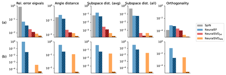
Figure 6: Summary of quantitative evaluations for solving TISEs: (a) 2D hydrogen atom; (b) 2D harmonic oscillator. Non-hatched, light-colored bars represent batch size of 128, while hatched bars indicate batch size of 512. The definitions of reported measures are given in Sec. F.1.3.

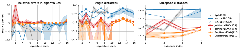
(a)

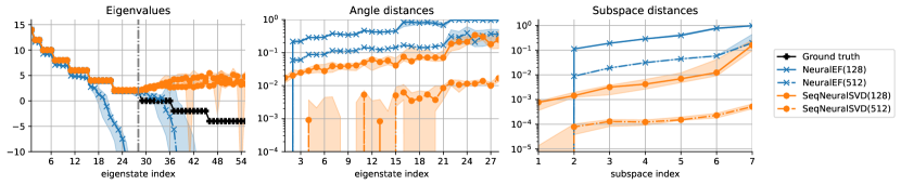
(b)

Figure 7: Quantitative evaluations of the learned eigenfunctions. The shaded region indicates 20% and 80% quantiles with respect to 10 random seeds. In the first panel of (b), the left of the black vertical line indicates the positive eigenvalues.

Remark on Shifting.

We note that the shifting technique can be applied to similar non-compact operators in general. Since the underlying spectrum is unknown in practice, the shifting parameter $c$ might be tuned by trial and error. We emphasize that the zero-norm property of NeuralSVD for non-positive part would be particularly useful, when the underlying spectrum is unknown.

Since any $c$ beyond a certain threshold makes the first $L$ modes with strictly positive eigenvalues for a fixed number of modes $L$, one may ask whether using larger $c$ is always a safe choice. If $c$ is too large, the shifted operator $\mathpzc{T}+c\mathpzc{I}$ is dominated by the identity operator, which admits any set of orthonormal functions as its orthonormal eigenbasis. In

F.1.3 Definitions of Reported Measures

We first provide the definitions of the reported measures in Fig. 4 and 7.

• Relative errors in eigenvalues: Given a learned eigenfunction $\tilde{\psi}_{\ell}(x)$, we estimate the learned eigenvalue by the Rayleigh quotient

  $$\tilde{\lambda}_{\ell}\mathrel{\mathop{\mathchar 58\relax missing}}=\frac{\langle\tilde{\psi}_{\ell}\mathchoice{\mspace{1.0mu}|\mspace{1.0mu}}{|}{|}{|}\mathpzc{T}\tilde{\psi}_{\ell}\rangle}{\langle\tilde{\psi}_{\ell}\mathchoice{\mspace{1.0mu}|\mspace{1.0mu}}{|}{|}{|}\tilde{\psi}_{\ell}\rangle},$$

  where each inner product is computed by importance sampling with finite samples from a given sampling distribution; see Appendix E.3. For each $\ell$, we then report the absolute relative error

  $$\frac{(\tilde{\lambda}_{\ell}-\lambda_{\ell})}{\lambda_{\ell}}\times 100~{}(\%),$$

  for $\lambda_{\ell}>0$.

• Angle distances: When there is degeneracy, i.e., several eigenstates share same eigenvalue, we need to align the learned functions within each subspace before we evaluate the performance eigenstate-wise. For such an alignment, we use the orthogonal Procrustes (OP) procedure defined as follows. Suppose that $\mathsf{A}\in\mathbb{R}^{N\times K}$ and $\mathsf{B}\in\mathbb{R}^{N\times K}$ are given. We wish to find the find the orthogonal transformation $\mathsf{A}\mathsf{\Omega}$ that best approximates the reference $\mathsf{B}$. The OP procedure defines the optimal $\mathsf{\Omega}^{\star}$ by the optimization problem

  $${\underset{\mathsf{\Omega}\in\mathbb{R}^{K\times K}}{\text{minimize}}} \|\mathsf{A}\mathsf{\Omega}-\mathsf{B}\|_{F}$$

  subject to $$\mathsf{\Omega}^{\intercal}\mathsf{\Omega}=I.$$

  The solution is characterized by the SVD of $\mathsf{A}^{\intercal}\mathsf{B}\in\mathbb{R}^{K\times K}$. If $\mathsf{A}^{\intercal}\mathsf{B}=\mathsf{U}\mathsf{S}\mathsf{V}^{\intercal}$ is the SVD, then $\mathsf{\Omega}^{\star}=\mathsf{U}\mathsf{V}^{\intercal}$. In our case, $\mathsf{A}$ is the vertical stack of the learned eigenfunctions and $\mathsf{B}$ is that of the ground truth eigenfunctions that correspond to a degenerate eigensubspace. Here, $K$ is the number of degeneracy and $N$ is the number of points used for the alignment.

  Given the aligned learned function $\bar{\psi}_{\ell}(x)$, we report the normalized angle distance

  $$\angle(\mathchoice{\mspace{1.0mu}|\mspace{1.0mu}}{|}{|}{|}\bar{\psi}_{\ell}\rangle,\mathchoice{\mspace{1.0mu}|\mspace{1.0mu}}{|}{|}{|}{\psi}_{\ell}\rangle)\mathrel{\mathop{\mathchar 58\relax missing}}=\frac{2}{\pi}\arccos\mathchoice{\mspace{1.0mu}|\mspace{1.0mu}}{|}{|}{|}\langle\psi_{\ell}\mathchoice{\mspace{1.0mu}|\mspace{1.0mu}}{|}{|}{|}\bar{\psi}_{\ell}\rangle\mathchoice{\mspace{1.0mu}|\mspace{1.0mu}}{|}{|}{|}\in[0,1].$$

  Here, we assume that both $\mathchoice{\mspace{1.0mu}|\mspace{1.0mu}}{|}{|}{|}\bar{\psi}_{\ell}\rangle$ and $\mathchoice{\mspace{1.0mu}|\mspace{1.0mu}}{|}{|}{|}{\psi}_{\ell}\rangle$ are normalized.

• Subspace distances: Another standard quantitative measure is the subspace distance defined as follows. Given $\mathsf{A}\in\mathbb{R}^{N\times K}$ and $\mathsf{B}\in\mathbb{R}^{N\times K}$, the normalized subspace distance between the column subspaces of the two matrices is defined as

  $$d(\mathsf{A},\mathsf{B})\mathrel{\mathop{\mathchar 58\relax missing}}=1-\frac{1}{K}\mathop{\rm tr}\nolimits(\mathsf{P}\mathsf{Q}),$$

  where $\mathsf{P}=\mathsf{A}(\mathsf{A}^{\intercal}\mathsf{A})^{-1}\mathsf{A}^{\intercal}\in\mathbb{R}^{N\times N}$ and $\mathsf{Q}=\mathsf{B}(\mathsf{B}^{\intercal}\mathsf{B})^{-1}\mathsf{B}^{\intercal}\in\mathbb{R}^{N\times N}$ are the projection matrices onto the column subspaces of $\mathsf{A}$ and $\mathsf{B}$, respectively. We note that $\mathsf{A}$ and $\mathsf{B}$ correspond to the learned and ground truth eigenfunctions that correspond to a given subspace as above.

The reported measures in Fig. 6 are averaged versions of the quantities defined above, except the orthogonality.

• Relative errors in eigenvalues: Report the average of the absolute relative errors over the eigenstates.

• Angle distance: Report the average of the angle distances over the eigenstates.

• Subspace distance: Report the average of the subspace distances over the degenerate subspaces.

• Orthogonality: To measure the orthogonality of the learned eigenfunctions, we report

  $$\frac{1}{N^{2}}\sum_{\ell=1}^{L}\sum_{\ell^{\prime}=1}^{L}(\langle\tilde{\psi}_{\ell}\mathchoice{\mspace{1.0mu}|\mspace{1.0mu}}{|}{|}{|}\tilde{\psi}_{\ell^{\prime}}\rangle-\delta_{\ell\ell^{\prime}})^{2}.$$

F.2 Cross-Domain Retrieval with Canonical Dependence Kernel

We used the Sketchy Extended dataset [37, 38] to train and evaluate our framework. There are total 75,479 sketches ($x$) and 73,002 photos ($y$) from 125 different classes.

We followed the standard training setup in the literature [40].

• Sampling distribution. As described in the main text, we define a sampling distribution as follows. First, note that we are given (empirical) class-conditional distributions $\{p(x\mathchoice{\mspace{1.0mu}|\mspace{1.0mu}}{|}{|}{|}c)\}_{c=1}^{K}$ and $\{p(y\mathchoice{\mspace{1.0mu}|\mspace{1.0mu}}{|}{|}{|}c)\}_{c=1}^{K}$ for each class $c\in[K]$. Given the (empirical) class distribution $p(c)$, we define the joint distribution

  $$p(x,y)\mathrel{\mathop{\mathchar 58\relax missing}}=\operatorname{\mathsf{E}}_{p(c)}[p(x\mathchoice{\mspace{1.0mu}|\mspace{1.0mu}}{|}{|}{|}C)p(y\mathchoice{\mspace{1.0mu}|\mspace{1.0mu}}{|}{|}{|}C)].$$

  That is, in practice, to draw a sample from $p(x,y)$, we can draw $C\sim p(c)$, and draw $(X,Y)\sim p(x\mathchoice{\mspace{1.0mu}|\mspace{1.0mu}}{|}{|}{|}C)p(y\mathchoice{\mspace{1.0mu}|\mspace{1.0mu}}{|}{|}{|}C)$.

• Pretrained fetures. We used a pretrained VGG16 network [89] to extract features of the sketches and images. The pretrained VGG network and train-test splits for evaluation are from the codebase of [90]. Hence, each sketch and photo is represented by a 512-dim. feature from the VGG network.

• Architecture. Treating the 512-dim. pretrained features as input, we used a single one-layer MLP of 8192 hidden units whose output dimension is 512. At the end of the network, we regularized the output so that the norm of the output has $\ell_{2}$-norm less than equal to $\mu=16$, i.e., $\|{\bf f}(x)\|_{2}\leq\mu$ for every $x$.

• Optimization. We trained the network for 10 epochs with batch size of 4096. We used the SGD optimizer with learning rate $5\times 10^{-3}$ and momentum $0.9$, together with the cosine learning rate schedule [88].

References

- Markovsky [2012] Ivan Markovsky. Low rank approximation: algorithms, implementation, applications, volume 906. Springer, 2012.
- Blum et al. [2020] Avrim Blum, John Hopcroft, and Ravindran Kannan. Foundations of data science. Cambridge University Press, 2020.
- Schölkopf et al. [1998] Bernhard Schölkopf, Alexander Smola, and Klaus-Robert Müller. Nonlinear component analysis as a kernel eigenvalue problem. Neural Comput., 10(5):1299–1319, 1998.
- Tenenbaum et al. [2000] Joshua B Tenenbaum, Vin De Silva, and John C Langford. A global geometric framework for nonlinear dimensionality reduction. Science, 290(5500):2319–2323, 2000.
- Roweis and Saul [2000] Sam T Roweis and Lawrence K Saul. Nonlinear dimensionality reduction by locally linear embedding. Science, 290(5500):2323–2326, 2000.
- Shi and Malik [2000] Jianbo Shi and Jitendra Malik. Normalized cuts and image segmentation. IEEE Trans. Pattern Anal. Mach. Intell., 22(8):888–905, 2000.
- Ng et al. [2001] Andrew Ng, Michael Jordan, and Yair Weiss. On spectral clustering: Analysis and an algorithm. In Adv. Neural Inf. Proc. Syst., volume 14, pages 849–856, 2001.
- Belkin and Niyogi [2003] Mikhail Belkin and Partha Niyogi. Laplacian eigenmaps for dimensionality reduction and data representation. Neural Comput., 15(6):1373–1396, 2003.
- Bengio et al. [2003] Yoshua Bengio, Pascal Vincent, Jean-François Paiement, Olivier Delalleau, Marie Ouimet, and Nicolas Le Roux. Spectral clustering and kernel PCA are learning eigenfunctions, volume 1239. CIRANO, 2003.
- Cox and Cox [2008] Michael AA Cox and Trevor F Cox. Multidimensional scaling. In Handbook of data visualization, pages 315–347. Springer, 2008.
- Michaeli et al. [2016] Tomer Michaeli, Weiran Wang, and Karen Livescu. Nonparametric canonical correlation analysis. In Proc. Int. Conf. Mach. Learn., pages 1967–1976, 2016.
- Wang et al. [2019] Lichen Wang, Jiaxiang Wu, Shao-Lun Huang, Lizhong Zheng, Xiangxiang Xu, Lin Zhang, and Junzhou Huang. An Efficient Approach to Informative Feature Extraction from Multimodal Data. In Proc. AAAI Conf. Artif. Int., volume 33, pages 5281–5288, July 2019. doi: 10.1609/aaai.v33i01.33015281.
- Andrews and Patterson [1976] Harry Andrews and C Patterson. Singular value decompositions and digital image processing. IEEE Trans. Acoust. Speech Signal Process., 24(1):26–53, 1976.
- Turk and Pentland [1991] Matthew Turk and Alex Pentland. Eigenfaces for recognition. J. Cogn. Neurosci., 3(1):71–86, 1991.
- Wiskott and Sejnowski [2002] Laurenz Wiskott and Terrence J Sejnowski. Slow feature analysis: Unsupervised learning of invariances. Neural Comput., 14(4):715–770, 2002.
- Sprekeler [2011] Henning Sprekeler. On the relation of slow feature analysis and Laplacian eigenmaps. Neural Comput., 23(12):3287–3302, 2011.
- Scetbon et al. [2021] Meyer Scetbon, Michael Elad, and Peyman Milanfar. Deep k-svd denoising. IEEE Trans. Image Proc., 30:5944–5955, 2021.
- Landauer et al. [1998] Thomas K Landauer, Peter W Foltz, and Darrell Laham. An introduction to latent semantic analysis. Discourse Process., 25(2-3):259–284, 1998.
- Goldberg and Levy [2014] Yoav Goldberg and Omer Levy. word2vec explained: deriving mikolov et al.’s negative-sampling word-embedding method. arXiv preprint arXiv:1402.3722, 2014.
- Hermann et al. [2020] Jan Hermann, Zeno Schätzle, and Frank Noé. Deep-neural-network solution of the electronic Schrödinger equation. Nat. Chem., 12(10):891–897, October 2020. ISSN 1755-4330, 1755-4349. doi: 10.1038/s41557-020-0544-y.
- Pfau et al. [2020] David Pfau, James S Spencer, Alexander G D G Matthews, and W M C Foulkes. Ab initio solution of the many-electron Schrödinger equation with deep neural networks. Phys. Rev. Res., 2(3):033429, September 2020. doi: 10.1103/PhysRevResearch.2.033429.
- Golub and Van Loan [2013] Gene H Golub and Charles F Van Loan. Matrix computations. JHU press, 2013.
- Williams and Seeger [2000] Christopher Williams and Matthias Seeger. Using the Nyström method to speed up kernel machines. In Adv. Neural Inf. Proc. Syst., volume 13, 2000.
- Bengio et al. [2004] Yoshua Bengio, Olivier Delalleau, Nicolas Le Roux, Jean-François Paiement, Pascal Vincent, and Marie Ouimet. Learning eigenfunctions links spectral embedding and kernel pca. Neural Comput., 16(10):2197–2219, 2004.
- Schmidt [1907] Erhard Schmidt. Zur Theorie der linearen und nichtlinearen Integralgleichungen. Math. Ann., 63(4):433–476, December 1907. ISSN 0025-5831, 1432-1807. doi: 10.1007/BF01449770.
- Pfau et al. [2019] David Pfau, Stig Petersen, Ashish Agarwal, David GT Barrett, and Kimberly L Stachenfeld. Spectral inference networks: Unifying deep and spectral learning. In Int. Conf. Learn. Repr., 2019.
- Deng et al. [2022a] Zhijie Deng, Jiaxin Shi, and Jun Zhu. NeuralEF: Deconstructing kernels by deep neural networks. In Kamalika Chaudhuri, Stefanie Jegelka, Le Song, Csaba Szepesvari, Gang Niu, and Sivan Sabato, editors, Proc. Int. Conf. Mach. Learn., volume 162 of Proceedings of Machine Learning Research, pages 4976–4992. PMLR, 17–23 Jul 2022a. URL https://proceedings.mlr.press/v162/deng22b.html.
- Gemp et al. [2021] Ian Gemp, Brian McWilliams, Claire Vernade, and Thore Graepel. EigenGame: PCA as a Nash equilibrium. In Int. Conf. Learn. Repr., 2021.
- Eckart and Young [1936] Carl Eckart and Gale Young. The approximation of one matrix by another of lower rank. Psychometrika, 1(3):211–218, September 1936. ISSN 0033-3123, 1860-0980. doi: 10.1007/BF02288367.
- Griffiths and Schroeter [2018] David J Griffiths and Darrell F Schroeter. Introduction to quantum mechanics. Cambridge university press, 2018.
- Wu et al. [2023] J Wu, S F Wang, and P Perdikaris. A dive into spectral inference networks: improved algorithms for self-supervised learning of continuous spectral representations. Appl. Math. Mech., 44(7):1199–1224, July 2023. ISSN 0253-4827, 1573-2754. doi: 10.1007/s10483-023-2998-7.
- Huang et al. [2019] Shao-Lun Huang, Anuran Makur, Gregory W Wornell, and Lizhong Zheng. On universal features for high-dimensional learning and inference. arXiv preprint arXiv:1911.09105, 2019.
- Xu and Zheng [2023] Xiangxiang Xu and Lizhong Zheng. A geometric framework for neural feature learning. arXiv preprint arXiv:2309.10140, 2023.
- Hirschfeld [1935] H O Hirschfeld. A Connection between Correlation and Contingency. Math. Proc. Cambridge Philos. Soc., 31(4):520–524, October 1935. ISSN 1469-8064, 0305-0041. doi: 10.1017/S0305004100013517.
- Gebelein [1941] Hans Gebelein. Das statistische Problem der Korrelation als Variations- und Eigenwertproblem und sein Zusammenhang mit der Ausgleichsrechnung. ZAMM Z. Angew. Math. Mech., 21(6):364–379, 1941. ISSN 0044-2267, 1521-4001. doi: 10.1002/zamm.19410210604.
- Rényi [1959] A Rényi. On measures of dependence. Acta Math. Hungarica, 10(3):441–451, September 1959. ISSN 1588-2632. doi: 10.1007/BF02024507.
- Sangkloy et al. [2016] Patsorn Sangkloy, Nathan Burnell, Cusuh Ham, and James Hays. The sketchy database: Learning to retrieve badly drawn bunnies. ACM Trans. Graph. (Proc. SIGGRAPH), 2016.
- Liu et al. [2017] Li Liu, Fumin Shen, Yuming Shen, Xianglong Liu, and Ling Shao. Deep sketch hashing: Fast free-hand sketch-based image retrieval. In Proc. IEEE Comput. Soc. Conf. Comput. Vis. Pattern Recognit., pages 2862–2871, 2017.
- Lin et al. [2020] Kaiyi Lin, Xing Xu, Lianli Gao, Zheng Wang, and Heng Tao Shen. Learning cross-aligned latent embeddings for zero-shot cross-modal retrieval. In Proc. AAAI Conf. Artif. Int., volume 34, pages 11515–11522, 2020.
- Hwang et al. [2020] HyeongJoo Hwang, Geon-Hyeong Kim, Seunghoon Hong, and Kee-Eung Kim. Variational interaction information maximization for cross-domain disentanglement. In Adv. Neural Inf. Proc. Syst., volume 33, 2020.
- Yelamarthi et al. [2018] Sasi Kiran Yelamarthi, Shiva Krishna Reddy, Ashish Mishra, and Anurag Mittal. A zero-shot framework for sketch based image retrieval. In Proc. Eur. Conf. Comput. Vis., pages 300–317, 2018.
- Bolla [2013] Marianna Bolla. Spectral clustering and biclustering: Learning large graphs and contingency tables. John Wiley & Sons, 2013.
- Trefethen and Bau [2022] Lloyd N Trefethen and David Bau. Numerical linear algebra, volume 181. SIAM, 2022.
- Stewart [2011] G W Stewart. Fredholm, Hilbert, Schmidt: three fundamental papers on integral equations. , 2011. URL http://users.umiacs.umd.edu/~stewart/FHS.pdf.
- Mirsky [1960] L Mirsky. Symmetric gauge functions and unitarily invariant norms. Q. J. Math., 11(1):50–59, January 1960. ISSN 0033-5606. doi: 10.1093/qmath/11.1.50.
- Stewart [1993] G W Stewart. On the early history of the singular value decomposition. SIAM Rev. Soc. Ind. Appl. Math., 35(4):551–566, December 1993. ISSN 0036-1445, 1095-7200. doi: 10.1137/1035134.
- Greenacre [1984] Michael J Greenacre. Theory and applications of correspondence analysis. London (UK) Academic Press, 1984.
- Hsu et al. [2019] Hsiang Hsu, Salman Salamatian, and Flavio P Calmon. Correspondence Analysis Using Neural Networks. In Int. Conf. Artif. Int. Statist., February 2019.
- Hsu et al. [2022] Hsiang Hsu, Salman Salamatian, and Flavio P Calmon. Generalizing Correspondence Analysis for Applications in Machine Learning. IEEE Trans. Pattern Anal. Mach. Intell., 44(12):9347–9362, December 2022. ISSN 0162-8828. doi: 10.1109/TPAMI.2021.3127870.
- HaoChen et al. [2021] Jeff Z HaoChen, Colin Wei, Adrien Gaidon, and Tengyu Ma. Provable guarantees for self-supervised deep learning with spectral contrastive loss. In Adv. Neural Inf. Proc. Syst., 2021.
- Tsai et al. [2020] Yao-Hung Hubert Tsai, Yue Wu, Ruslan Salakhutdinov, and Louis-Philippe Morency. Self-supervised learning from a multi-view perspective. In Int. Conf. Learn. Repr., 2020.
- Xu et al. [2022] Xiangxiang Xu, Shao-Lun Huang, Lizhong Zheng, and Gregory W Wornell. An information theoretic interpretation to deep neural networks. Entropy, 24(1):135, 2022.
- Hu and Principe [2022] Bo Hu and Jose C Principe. The cross density kernel function: A novel framework to quantify statistical dependence for random processes. arXiv preprint arXiv:2212.04631, 2022.
- Sanger [1989] Terence D Sanger. Optimal unsupervised learning in a single-layer linear feedforward neural network. Neural Netw., 2(6):459–473, January 1989. ISSN 0893-6080. doi: 10.1016/0893-6080(89)90044-0.
- Kusupati et al. [2022] Aditya Kusupati, Gantavya Bhatt, Aniket Rege, Matthew Wallingford, Aditya Sinha, Vivek Ramanujan, William Howard-Snyder, Kaifeng Chen, Sham Kakade, Prateek Jain, and Ali Farhadi. Matryoshka representation learning. In Adv. Neural Inf. Proc. Syst., volume 35, pages 30233–30249, 2022.
- Andrew et al. [2013] Galen Andrew, Raman Arora, Jeff Bilmes, and Karen Livescu. Deep canonical correlation analysis. In Proc. Int. Conf. Mach. Learn., pages 1247–1255. PMLR, 2013.
- Lagaris et al. [1997] I E Lagaris, A Likas, and D I Fotiadis. Artificial neural network methods in quantum mechanics. Comput. Phys. Commun., 104(1-3):1–14, August 1997. ISSN 0010-4655, 1879-2944. doi: 10.1016/s0010-4655(97)00054-4.
- Bar and Sochen [2019] Leah Bar and Nir Sochen. Unsupervised Deep Learning Algorithm for PDE-based Forward and Inverse Problems. arXiv, April 2019.
- Ben-Shaul et al. [2023] Ido Ben-Shaul, Leah Bar, Dalia Fishelov, and Nir Sochen. Deep Learning Solution of the Eigenvalue Problem for Differential Operators. Neural Comput., 35(6):1100–1134, May 2023. ISSN 0899-7667, 1530-888X. doi: 10.1162/neco_a_01583.
- Li et al. [2021a] Hong Li, Qilong Zhai, and Jeff Z Y Chen. Neural-network-based multistate solver for a static Schrödinger equation. Phys. Rev. A, 103(3):032405, March 2021a. ISSN 1050-2947. doi: 10.1103/PhysRevA.103.032405.
- Zhang et al. [2022] Wei Zhang, Tiejun Li, and Christof Schütte. Solving eigenvalue PDEs of metastable diffusion processes using artificial neural networks. J. Comput. Phys., 465:111377, September 2022. ISSN 0021-9991. doi: 10.1016/j.jcp.2022.111377.
- Liu et al. [2023] Jinde Liu, Xilong Dou, Xi He, Chen Yang, and Gang Jiang. Calculating many excited states of the multidimensional time-independent Schrödinger equation using a neural network. Phys. Rev. A, 108(3):032803, September 2023. ISSN 1050-2947. doi: 10.1103/PhysRevA.108.032803.
- Wang and Xie [2023] Yifan Wang and Hehi Xie. Computing Multi-Eigenpairs of High-Dimensional Eigenvalue Problems Using Tensor Neural Networks. arXiv, May 2023.
- Guo and Ming [2023] Yixiao Guo and Pingbing Ming. A Deep Learning Method for Computing Eigenvalues of the Fractional Schrödinger Operator. arXiv, August 2023.
- Mattheakis et al. [2022] Marios Mattheakis, Gabriel R Schleder, Daniel T Larson, and Efthimios Kaxiras. First principles physics-informed neural network for quantum wavefunctions and eigenvalue surfaces. In Machine Learning and the Physical Sciences workshop, December 2022.
- Jin et al. [2020] Henry Jin, Marios Mattheakis, and Pavlos Protopapas. Unsupervised Neural Networks for Quantum Eigenvalue Problems. arXiv, October 2020.
- Jin et al. [2022] Henry Jin, Marios Mattheakis, and Pavlos Protopapas. Physics-Informed Neural Networks for Quantum Eigenvalue Problems. In Proc. Int. Jt. Conf. Neural Netw., pages 1–8, July 2022. doi: 10.1109/IJCNN55064.2022.9891944.
- Holliday et al. [2023] Elliott G Holliday, John F Lindner, and William L Ditto. Solving two-dimensional quantum eigenvalue problems using physics-informed machine learning. arXiv, February 2023.
- Han et al. [2020] Jiequn Han, Jianfeng Lu, and Mo Zhou. Solving high-dimensional eigenvalue problems using deep neural networks: A diffusion Monte Carlo like approach. J. Comput. Phys., 423(109792):109792, December 2020. ISSN 0021-9991, 1090-2716. doi: 10.1016/j.jcp.2020.109792.
- Yang et al. [2023] Qihong Yang, Yangtao Deng, Yu Yang, Qiaolin He, and Shiquan Zhang. Neural networks based on power method and inverse power method for solving linear eigenvalue problems. Comput. Math. Appl., 147:14–24, October 2023. ISSN 0898-1221. doi: 10.1016/j.camwa.2023.07.013.
- Li and Ying [2021] Haoya Li and Lexing Ying. A semigroup method for high dimensional elliptic PDEs and eigenvalue problems based on neural networks. arXiv, May 2021.
- E and Yu [2018] Weinan E and Bing Yu. The deep Ritz method: a deep learning-based numerical algorithm for solving variational problems. Commun Math Stat., 6(1):1–12, 2018.
- Sirignano and Spiliopoulos [2018] Justin Sirignano and Konstantinos Spiliopoulos. DGM: A deep learning algorithm for solving partial differential equations. J. Comput. Phys., 375:1339–1364, 2018.
- Li et al. [2021b] Zongyi Li, Nikola Kovachki, Kamyar Azizzadenesheli, Burigede Liu, Kaushik Bhattacharya, Andrew Stuart, and Anima Anandkumar. Fourier neural operator for parametric partial differential equations. In Int. Conf. Learn. Repr., 2021b.
- Carleo and Troyer [2017] Giuseppe Carleo and Matthias Troyer. Solving the quantum many-body problem with artificial neural networks. Science, 355(6325):602–606, February 2017. ISSN 0036-8075, 1095-9203. doi: 10.1126/science.aag2302.
- Schütt et al. [2017] Kristof Schütt, Pieter-Jan Kindermans, Huziel Enoc Sauceda Felix, Stefan Chmiela, Alexandre Tkatchenko, and Klaus-Robert Müller. Schnet: A continuous-filter convolutional neural network for modeling quantum interactions. In I. Guyon, U. Von Luxburg, S. Bengio, H. Wallach, R. Fergus, S. Vishwanathan, and R. Garnett, editors, Adv. Neural Inf. Proc. Syst., volume 30. Curran Associates, Inc., 2017. URL https://proceedings.neurips.cc/paper_files/paper/2017/file/303ed4c69846ab36c2904d3ba8573050-Paper.pdf.
- Choo et al. [2020] Kenny Choo, Antonio Mezzacapo, and Giuseppe Carleo. Fermionic neural-network states for ab-initio electronic structure. Nat. Commun., 11(1):2368, May 2020. ISSN 2041-1723. doi: 10.1038/s41467-020-15724-9.
- Gerard et al. [2022] Leon Gerard, Michael Scherbela, Philipp Marquetand, and Philipp Grohs. Gold-standard solutions to the Schrödinger equation using deep learning: How much physics do we need? In Adv. Neural Inf. Proc. Syst., December 2022.
- Hermann et al. [2022] Jan Hermann, James Spencer, Kenny Choo, Antonio Mezzacapo, W M C Foulkes, David Pfau, Giuseppe Carleo, and Frank Noé. Ab-initio quantum chemistry with neural-network wavefunctions. arXiv, August 2022.
- Cuzzocrea et al. [2020] Alice Cuzzocrea, Anthony Scemama, Wim J Briels, Saverio Moroni, and Claudia Filippi. Variational Principles in Quantum Monte Carlo: The Troubled Story of Variance Minimization. J. Chem. Theory Comput., 16(7):4203–4212, July 2020. ISSN 1549-9618, 1549-9626. doi: 10.1021/acs.jctc.0c00147.
- Entwistle et al. [2023] M T Entwistle, Z Schätzle, P A Erdman, J Hermann, and F Noé. Electronic excited states in deep variational Monte Carlo. Nat. Commun., 14(1):274, January 2023. ISSN 2041-1723. doi: 10.1038/s41467-022-35534-5.
- Pfau et al. [2023] David Pfau, Simon Axelrod, Halvard Sutterud, Ingrid von Glehn, and James S Spencer. Natural Quantum Monte Carlo Computation of Excited States. arXiv, August 2023.
- Deng et al. [2022b] Zhijie Deng, Jiaxin Shi, Hao Zhang, Peng Cui, Cewu Lu, and Jun Zhu. Neural Eigenfunctions Are Structured Representation Learners. arXiv, October 2022b.
- Gemp et al. [2022] Ian Gemp, Brian McWilliams, Claire Vernade, and Thore Graepel. EigenGame unloaded: When playing games is better than optimizing. In Int. Conf. Learn. Repr., 2022. URL https://openreview.net/forum?id=So6YAqnqgMj.
- Yang et al. [1991] X L Yang, S H Guo, F T Chan, K W Wong, and W Y Ching. Analytic solution of a two-dimensional hydrogen atom. I. Nonrelativistic theory. Phys. Rev. A, 43(3):1186–1196, February 1991. ISSN 1050-2947. doi: 10.1103/physreva.43.1186.
- Tancik et al. [2020] Matthew Tancik, Pratul Srinivasan, Ben Mildenhall, Sara Fridovich-Keil, Nithin Raghavan, Utkarsh Singhal, Ravi Ramamoorthi, Jonathan Barron, and Ren Ng. Fourier features let networks learn high frequency functions in low dimensional domains. In Adv. Neural Inf. Proc. Syst., volume 33, pages 7537–7547, 2020.
- Hinton et al. [2012] Geoffrey Hinton, Nitish Srivastava, and Kevin Swersky. Neural networks for machine learning lecture 6a overview of mini-batch gradient descent. , 2012.
- Loshchilov and Hutter [2016] Ilya Loshchilov and Frank Hutter. SGDR: Stochastic gradient descent with warm restarts. arXiv preprint arXiv:1608.03983, 2016.
- Simonyan and Zisserman [2015] Karen Simonyan and Andrew Zisserman. Very deep convolutional networks for large-scale image recognition. In Int. Conf. Learn. Repr., 2015.
- Dutta and Akata [2019] Anjan Dutta and Zeynep Akata. Semantically tied paired cycle consistency for zero-shot sketch-based image retrieval. In Proc. IEEE Comput. Soc. Conf. Comput. Vis. Pattern Recognit., pages 5089–5098, 2019.