Revisiting the Dataset Bias Problem from a Statistical Perspective

Abstract

In this paper, we study the “dataset bias” problem from a statistical standpoint, and identify the main cause of the problem as the strong correlation between a class attribute $u$ and a non-class attribute $b$ in the input $x$, represented by $p(u|b)$ differing significantly from $p(u)$. Since $p(u|b)$ appears as part of the sampling distributions in the standard maximum log-likelihood (MLL) objective, a model trained on a biased dataset via MLL inherently incorporates such correlation into its parameters, leading to poor generalization to unbiased test data. From this observation, we propose to mitigate dataset bias via either weighting the objective of each sample $n$ by $\frac{1}{p(u_{n}|b_{n})}$ or sampling that sample with a weight proportional to $\frac{1}{p(u_{n}|b_{n})}$. While both methods are statistically equivalent, the former proves more stable and effective in practice. Additionally, we establish a connection between our debiasing approach and causal reasoning, reinforcing our method’s theoretical foundation. However, when the bias label is unavailable, computing $p(u|b)$ exactly is difficult. To overcome this challenge, we propose to approximate $\frac{1}{p(u|b)}$ using a biased classifier trained with “bias amplification” losses. Extensive experiments on various biased datasets demonstrate the superiority of our method over existing debiasing techniques in most settings, validating our theoretical analysis.

1 Introduction

In recent years, Deep Neural Networks (DNNs) have achieved remarkable performance in Computer Vision and Natural Language Processing tasks. This success can be attributed to their capability of capturing various patterns in the training data that are indicative of the target class. However, when the training data exhibits strong correlation between a non-class attribute and the target class (often referred to as “dataset bias” [3, 5, 35, 46]), DNNs may overly rely on the non-class attribute instead of the actual class attribute, especially if the non-class attribute is easier to learn [46]. This leads to biased models that struggle to generalize to new scenarios where the training bias is absent. For instance, consider a dataset of human face images where men typically have black hair and women usually have blond hair. If we train a DNN on this dataset for gender classification, the model might take a “shortcut” and use hair color (a non-class attribute) as a primary predictor. As a result, when the model encounters a man with blond hair during testing, it erroneously predicts the individual as a woman.

To tackle the dataset bias problem, earlier approaches rely on the availability of bias labels [29]. They employ supervised learning to train a bias prediction model to capture the bias in the training data, and concurrently learn debiased features that share the smallest mutual information with the captured bias. The debiased features are then utilized for predicting the target class. On the other hand, alternative approaches relax the assumption of bias label availability and focus on specific types of bias [5, 59]. They introduce specialized network architectures to capture these specific types of bias. For example, Bahng et al. [5] leverage convolutional networks with small receptive fields to capture textural bias in images. However, acquiring human annotations for bias can be laborious, expensive, and requires expertise in bias identification, making it challenging in practical scenarios. Furthermore, bias labeling may not encompass all forms of bias present in the training data, particularly those that are continuous. As a result, recent approaches have shifted their attention to settings where no prior knowledge about bias is available [3, 24, 30, 31, 37, 46]. Many of these methods exploit knowledge from a “biased” model trained by minimizing a “bias amplification” loss [64] to effectively mitigate bias [3, 37, 46]. They have achieved significant improvement in bias mitigation, even surpassing approaches that assume bias labels. However, the heuristic nature of their bias correction formulas makes it difficult to clearly understand why these methods perform well in practice.

In this paper, we revisit the dataset bias problem from a statistical perspective, and present a mathematical representation of this bias, expressed as either $p(u|b)\neq p(u)$ or $p(b|u)\neq p(b)$ where $u$, $b$ refer to the class attribute and non-class (bias) attribute, respectively. Our representation characterizes the common understanding of dataset bias as “high correlation between the bias attribute and class attribute” [5, 37]. In addition, we demonstrate that dataset bias arises naturally within the standard maximum log-likelihood objective as part of the sampling distribution, alongside the “imbalance bias”. Building on this insight, we propose two approaches to mitigate dataset bias: weighting the loss of each sample $n$ by $\frac{1}{p(u_{n}|b_{n})}$, or sampling the sample with a weight proportional to $\frac{1}{p(u_{n}|b_{n})}$. Through empirical analysis, we highlight the distinct behaviors of these methods, despite their statistical equivalence. Furthermore, we offer an intriguing perspective on dataset bias as a “confounding bias” in causal reasoning, and theoretically show that our method actually learns the causal relationship between the target class $y$ and the class attribute $u$ via minimizing an upper bound of the expected negative interventional log-likelihood $\mathbb{E}_{n}\left[-\log p_{\theta}(y_{n}|\text{do}(u_{n}))\right]$. However, accurately computing $\frac{1}{p(u_{n}|b_{n})}$ or $p(u_{n}|b_{n})$ poses a significant challenge when $b_{n}$ is unknown and intertwined with $u_{n}$ in the input $x_{n}$. To address this issue, we propose an alternative approach that approximates $p(y_{n}|b_{n})$, a proxy for $p(u_{n}|b_{n})$, using a biased classifier trained with “bias amplification” losses [46]. Our intuition is that if the biased classifier $p_{\psi}(y_{n}|x_{n})$ is properly trained to use only the bias attribute $b_{n}$ in the input $x_{n}$ for predicting $y_{n}$, then $p_{\psi}(y_{n}|x_{n})$ can serve as a reasonable approximation of $p(y_{n}|b_{n})$.

We conduct comprehensive experiments on four popular biased datasets that encompass various forms of bias: Colored MNIST, Corrupted CIFAR10, Biased CelebA, and BAR [46]. Experimental results show that our method achieves superior bias mitigation results compared to many existing baselines. This validates the soundness of our theoretical analysis and demonstrates the effectiveness of our method in mitigating bias, especially when no bias label is available. Additionally, our ablation studies reveal surprising alignments between the optimal configurations of our method and the values indicated by our theoretical analysis on some simple datasets like Colored MNIST.

2 A Statistical View of Dataset Bias

We consider the standard supervised learning problem which involves learning a classifier $p_{\theta}(y|x)$, parameterized by $\theta$, that maps an input sample $x$ to the class probability vector. Let $\mathcal{D}:=\left\{(x_{n},y_{n})\right\}_{n=1}^{N}$ denote the training dataset consisting of $N$ samples. The typical learning strategy minimizes the expected negative log-likelihood (NLL) of $y$ conditional on $x$, computed as follows:

$$\mathcal{L}_{\theta}^{\text{NLL}}:=\mathbb{E}_{p_{\mathcal{D}}(x_{n},y_{n})}\left[-\log p_{\theta}(y_{n}|x_{n})\right]$$ (1)

In the above equation, we intentionally include the subscript $n$ to emphasize that $x_{n}$ and $y_{n}$ correspond to a particular sample $n$ rather than being arbitrary. Without loss of generality, we assume that each input $x$ consists of two types of attributes: the class attribute (denoted by $u$) and the non-class attribute (denoted by $b$), i.e., $x=(u,b)$. For example, in the ColoredMNIST dataset [5, 46], $u$ represents the digit shape and $b$ represents the background color. Eq. 1 can be written as:

$$\mathcal{L}_{\theta}^{\text{NLL}} =\mathbb{E}_{p_{\mathcal{D}}(x_{n})p_{\mathcal{D}}(y_{n}|x_{n})}\left[-\log p_{\theta}(y_{n}|x_{n})\right]$$ (2)

$$=\mathbb{E}_{p_{\mathcal{D}}(x_{n})}\left[\mathcal{L}_{\theta}^{\text{xent}}(x_{n},y_{n})\right]$$ (3)

$$=\mathbb{E}_{p(u_{n})p(b_{n}|u_{n})}\left[\mathcal{L}_{\theta}^{\text{xent}}(x_{n},y_{n})\right]$$ (4)

$$=\mathbb{E}_{p(b_{n})p(u_{n}|b_{n})}\left[\mathcal{L}_{\theta}^{\text{xent}}(x_{n},y_{n})\right]$$ (5)

where $\mathcal{L}_{\theta}^{\text{xent}}$ denotes the cross-entropy loss. Intuitively, if $u$ is distinctive among classes, $u$ can be generally treated as a categorical random variable. In this case, we will have $p(u_{n})\approx p(y_{n})$ and $p(b_{n}|u_{n})\approx p(b_{n}|y_{n})$. From Eq. 4, it is clear that there are two main sources of bias in the training data. One comes from the non-uniform distribution of the class attribute (i.e., $p(u)$ is not uniform among classes), and the other comes from the strong correlation between the non-class attribute $b$ and the class attribute $u$ (i.e., $p(b|u)$ is very different from $p(b)$). A highly correlated non-class attribute will cause the model to depend more on $b$ and less on $u$ to predict $y$. The former is commonly known as the “class-imbalance bias”, while the latter is often referred to as the “dataset bias” [3, 5, 35, 46]. In this paper, we focus exclusively on addressing the dataset bias due to its difficulty, especially when no prior knowledge about the bias is available. Besides, we decide to rename the dataset bias as “feature-correlation bias” since we believe this name better characterizes the property of the bias. We also refer to $b$ as a bias attribute because it is the primary factor contributing to the bias. In the next section, we will discuss in detail our methods for mitigating the feature-correlation bias.

3 Mitigating Dataset Bias from Statistical and Causal Perspectives

3.1 Bias mitigation based on $p(u|b)$

Eq. 5 suggests that we can mitigate the dataset bias (or feature-correlation bias) by either weighting the individual loss $\mathcal{L}_{\theta}^{\text{xent}}(x_{n},y_{n})$ by $\frac{1}{p(u_{n}|b_{n})}$ during training or sampling each data point $(x_{n},y_{n})$ with the weight proportional to $\frac{1}{p(u_{n}|b_{n})}$. We refer to the two techniques as loss weighting (LW) and weighted sampling (WS), respectively. The two techniques are statistically equivalent, and transform the objective in Eq. 5 into $\mathbb{E}_{p(b_{n})}\left[\mathcal{L}_{\theta}^{\text{xent}}(x_{n},y_{n})\right]$, which no longer contains $p(u_{n}|b_{n})$.

We can approximate $p(u_{n}|b_{n})$ using its proxy $p(y_{n}|b_{n})$. However, explicitly modeling $p(y|b)$ pose challenges due to the typical unknown nature of $b$. Meanwhile, modeling $p(y|x)$ (or $p(y|u,b)$) is straightforward. Therefore, we propose to model $p(y|b)$ indirectly through $p(y|x)$ by training a parameterized model $p_{\psi}(y|x)$ in a manner that amplifies the influence of the bias attribute $b$ (in $x$) on $y$. We refer to $p_{\psi}(y|x)$ as the biased classifier and train it for $T_{\text{bias}}$ epochs using a bias amplification loss. Specifically, we choose the generalized cross-entropy (GCE) loss $\mathcal{L}_{\psi}^{\text{GCE}}(x_{n},y_{n})=\frac{1-{p_{\psi}(y_{n}|x_{n})}^{\tau}}{\tau}$ [64] where $\tau\in(0,1]$ is a hyperparameter controlling the degree of amplification. Once $p_{\psi}(y|x)$ has been trained, we can compute the weight for sample $n$ as follows:

$$w_{n}=\min\left(\frac{1}{p_{\psi}(y_{n}|x_{n})},\gamma\right)$$ (6)

where $\gamma>0$ is a clamp hyperparameter that prevents $w_{n}$ from becoming infinite when $p_{\psi}(y_{n}|x_{n})$ is close to 0. Since $p_{\psi}(y_{n}|x_{n})\in[0,1]$, $w_{n}\in[1,\gamma]$. $w_{n}$ can be considered as an approximation of $\frac{1}{p(u_{n}|b_{n})}$. For the debiasing purpose, we can train $p_{\theta}(y|x)$ via either loss weighting (LW) or weighted sampling (WS) with the weight $w_{n}$. In the case of LW, the debiasing loss becomes:

$$\mathcal{L}_{\theta}^{\text{LW}} =\mathbb{E}_{p(b_{n})p(u_{n}|b_{n})}\left[\frac{\mathcal{L}_{\theta}^{\text{xent}}(x_{n},y_{n})}{p(u_{n}|b_{n})}\right]$$ (7)

$$\approx\mathbb{E}_{p_{\mathcal{D}}(x_{n})}\left[w_{n}\cdot\mathcal{L}_{\theta}^{\text{xent}}(x_{n},y_{n})\right]$$ (8)

Although LW and WS are statistically equivalent, they perform differently in practice. LW preserves the diversity of training data but introduces different scales to the loss. To make training with LW stable, we rescale $w_{n}$ so that its maximum value is not $\gamma$ (which could be thousands) but a small constant value, which is 10 in this work. This means $w_{n}$ lies in the range $\left[\frac{10}{\gamma},10\right]$. WS, by contrast, maintains a constant scale of the loss but fails to ensure the diversity of training data due to over/under-sampling. During our experiment, we observed that LW often yields better performance than WS, which highlights the importance of data diversity.

However, if we simply fix the sample weight to be $w_{n}$ throughout training, a classifier trained via LW will take long time to achieve good results, and the results will be not optimal in some cases. It is because bias-aligned (BA) samples, which dominates the training data, have very small weights. The classifier will spend most of the training time performing very small updates on these BA samples, and thus, struggles to capture useful information in the training data. To deal with this problem, we propose a simple yet effective annealing strategy for LW. We initially set the weights of all training samples to the same value $\beta$ and linearly transform $\beta$ to $w_{n}$ for $T_{\text{anneal}}$ steps. Mathematically, the weight for sample $n$ at step $t$ is $w_{n}(t)=\begin{cases}\beta+\frac{t(w_{n}-\beta)}{T_{\text{anneal}}}&\text{if }0<t<T_{\text{anneal}}\\ w_{n}&\text{otherwise}\end{cases}$ and the loss for annealed loss weighting (ALW) is given below:

$$\mathcal{L}_{\theta}^{\text{ALW}}(t)=\mathbb{E}_{p_{\mathcal{D}}(x_{n})}\left[w_{n}(t)\cdot\mathcal{L}_{\theta}^{\text{xent}}(x_{n},y_{n})\right]$$ (9)

3.2 Interpretation of $\mathcal{L}_{\theta}^{\text{LW}}$ from a causal perspective

Figure 1: A causal graphical model representing the feature-correlation bias problem. $X$, $Y$ are the input image and class label, respectively. Both are observed (marked with shaded background) during training. $U$, $B$ are the hidden class and non-class attributes of $X$, respectively.

Interestingly, we can interpret the debiasing loss $\mathcal{L}_{\theta}^{\text{LW}}$ in the language of causal reasoning by utilizing the Potential Outcomes framework [52] illustrated in Fig. 1, where the class label $Y$, class attribute $U$, and non-class attribute $B$ play the roles of the outcome, treatment, and confounder, respectively. In our setting, both $U$ and $B$ are hidden but can be accessed through the observed input $X$. When the unconfoundedness and positivity assumptions (i.e. the backdoor assumptions) [61] are met, we can estimate the causal quantity $p(y|\text{do}(u))$ from observational data via backdoor adjustment [49] as follows:

$$p(y|\text{do}(u)) =\sum_{b}\frac{p(y,u,b)}{p(u|b)}$$ (10)

$$=\mathbb{E}_{p(u,b)}\left[\frac{p(y|u,b)}{p(u|b)}\right]$$ (11)

$$=\mathbb{E}_{p(b)}\left[p(y|u,b)\right]$$ (12)

Eq. 11 is typically known as Inverse Probability Weighting (IPW), where $p(u|b)$ is called the propensity score [21, 20]. In Eq. 11, the class prediction $p(y|u,b)$ is weighted by the inverse propensity score $\frac{1}{p(u|b)}$, exhibiting a degree of resemblance to our loss $\mathcal{L}_{\theta}^{\text{LW}}$ in Eq. 7. It suggests that we can interpret $\mathcal{L}_{\theta}^{\text{LW}}$ from a causal standpoint. In fact, $\mathcal{L}_{\theta}^{\text{LW}}$ acts as an upper bound of the expected negative interventional log-likelihood (NILL) $\mathcal{L}_{\theta}^{\text{NILL}}=\mathbb{E}_{n}\left[-\log p_{\theta}(y_{n}|\text{do}(u_{n}))\right]$. The relationship between these two losses is provided below:

$$\mathcal{L}_{\theta}^{\text{NILL}} =\mathbb{E}_{n}\left[-\log p_{\theta}(y_{n}|\text{do}(u_{n}))\right]$$ (13)

$$\leq\mathbb{E}_{p(u_{n},b_{n},y_{n})}\left[\frac{-\log p_{\theta}(y_{n}|u_{n},b_{n})}{p(u_{n}|b_{n})}\right]$$ (14)

$$=\mathbb{E}_{p(u_{n},b_{n})}\left[\frac{\mathcal{L}_{\theta}^{\text{xent}}(x_{n},y_{n})}{p(u_{n}|b_{n})}\right]=\mathcal{L}_{\theta}^{\text{LW}}$$ (15)

where the inequality in Eq. 14 is derived from:

$$-\log p_{\theta}(y|\text{do}(u)) =-\log\mathbb{E}_{p(b)}\left[p_{\theta}(y|u,b)\right]$$ (16)

$$\leq-\mathbb{E}_{p(b)}\left[\log p_{\theta}(y|u,b)\right]$$ (17)

$$=\mathbb{E}_{p(u,b)}\left[\frac{-\log p_{\theta}(y|u,b)}{p(u|b)}\right]$$ (18)

Eq. 17 is the Jensen inequality with equality attained when $p_{\theta}(y|u,b)=p_{\theta}(y|u,b^{\prime})$ $\forall$ $b,b^{\prime}$, i.e. $y$ is independent of $b$ given $u$. This condition matches our target of learning an unbiased classifier $p_{\theta}(y|u,b)$. In Eq. 18, $p(u|b)$ is introduced to allow $(u,b)$ to be sampled jointly from observational data. Eq. 14 can be viewed as a Monte Carlo estimation of Eq. 18 (or Eq. 17) using a single sample of $b$, i.e. $b_{n}$. From Eqs. 13 - 18, we see that minimizing $\mathcal{L}_{\theta}^{\text{LW}}$ also minimizes $\mathcal{L}_{\theta}^{\text{NILL}}$ and encourages $p_{\theta}(y|u,b)$ to be close to $p_{\theta}(y|u)$. Minimizing $\mathcal{L}_{\theta}^{\text{NILL}}$ causes the model to focus more (less) on uncommon (common) samples $n$ which has small (big) $p(u_{n}|b_{n})$.

3.3 Bias mitigation based on $p(b|u)$

Eq. 4 suggests an alternative approach to mitigating the feature-correlation bias, which involves weighting each individual sample $n$ by $\frac{1}{p(b_{n}|u_{n})}$ rather than $\frac{1}{p(u_{n}|b_{n})}$. However, accurately estimating $p(b|u)$ poses challenges in practical implementations. In Appdx. 3.1, we present an idea about using conditional generative models to approximate $p(b|u)$ and discuss its limitations.

4 Related Work

A plethora of techniques for mitigating bias are present in the literature. However, in this paper’s context, we focus on the most relevant and recent methods, leaving the discussion of other approaches in Appdx. A. These methods can be broadly categorized into two groups: i) those that utilize the bias label or prior knowledge about bias, and ii) those that do not. The two groups are discussed in detail below.

Debiasing given the bias label or certain types of bias

When the bias label is available, a straightforward approach is to train a bias prediction network or a “biased” network in a supervised manner. The bias knowledge acquired from the biased network can then be utilized as a form of regularization to train another “debiased” network. One commonly used regularization strategy involves minimizing the mutual information between the biased and debiased networks through adversarial training [5, 29, 66]. This compels the debiased network to learn features independent of the bias information, which are considered unbiased. In the model proposed by [29], a “biased” head is positioned on top of a “debiased” backbone with a gradient reversal layer [16] in between to facilitate adversarial learning. The backbone is trained to trick the biased head into predicting incorrect bias labels while the biased head attempts to make correct bias predictions. Other works, such as [5, 59], do not make use of the bias label; rather, they assume that image texture is the main source of bias. This comes from the observation that outputs of deep neural networks depend heavily on superficial statistics of the input image such as texture [17]. The framework in [59] consists of two branches: a conventional CNN for encoding visual features from the input image, and a set of learnable gray-level co-occurrence matrices (GLCMs) for extracting the textural bias information. Besides adversarial regularization, the authors of [59] introduce another regularization technique known as HEX, which projects the CNN features into a hidden space so that the projected vectors contain minimal information about the texture bias captured by the GLCM branch. [5], on the other hand, use a CNN with small receptive fields as the biased network, and the Hilbert-Schmidt Independence Criterion (HSIC) as a measure of mutual information between the biased and debiased classifiers’ features. [22] draw a probabilistic connection between data generated by $p(y)p(b)$ and by $p(y|b)p(b)$, and utilize the assumption that $p(x|y,b)$ remains unchanged regardless of the change in $p(y,b)$ to derive an effective bias correction method called BiasBal. They also propose BiasCon - a debiasing method based on contrastive learning. In the case the bias label is not provided, they assume the bias is texture and make use of the biased network proposed in [5]. EnD [55] employs a regularization loss for debiasing that comprises two terms: a “disentangling” term that promotes the decorrelation of samples with similar bias labels, and an “entangling” term which forces samples belonging to the same class but having different bias labels to be correlated. EnD exhibits certain similarities to BiasCon [22], as the “entangling” and “disentangling” terms can be viewed as the positive and negative components of a contrastive loss, respectively.

In visual question answering (VQA), bias can arise from the co-occurrence of words in the question and answer, causing the model to overlook visual cues when making predictions [1, 2]. To overcome this bias, common approaches involve training a biased network that takes only questions as input to predict answers. The prediction from this biased network is then used to modulate the prediction of a debiased network trained on both questions and images [8, 11, 50].

Dataset	BC (%)	Vanilla	ReBias	LfF	DFA	SelecMix	PGD	LW (Ours)
Colored MNIST	0.5	80.18$\pm$1.38	74.85$\pm$1.97	93.38$\pm$0.52	91.85$\pm$0.92	83.41$\pm$1.26	96.15$\pm$0.28	95.57$\pm$0.41
	1.0	87.48$\pm$1.75	84.23$\pm$1.56	94.09$\pm$0.78	94.32$\pm$0.89	91.59$\pm$0.99	97.93$\pm$0.19	97.18$\pm$0.34
	5.0	97.04$\pm$0.21	95.76$\pm$0.50	97.40$\pm$0.25	96.74$\pm$0.43	97.37$\pm$0.15	98.74$\pm$0.12	98.61$\pm$0.09
Corrupted CIFAR10	0.5	28.00$\pm$1.15	-	41.95$\pm$1.56	40.54$\pm$1.98	31.67$\pm$0.90	44.89$\pm$1.36	45.76$\pm$1.49
	1.0	34.56$\pm$0.87	-	53.36$\pm$1.87	50.27$\pm$0.94	36.28$\pm$1.22	47.38$\pm$1.01	51.64$\pm$1.12
	5.0	59.33$\pm$1.26	-	70.04$\pm$1.05	67.05$\pm$1.82	63.15$\pm$1.17	63.60$\pm$0.58	70.45$\pm$1.24

Table 1: Results of different debiasing methods on Colored MNIST and Corrupted CIFAR10 when the bias label is unavailable. The best and second best results are highlighted in bold and gray, respectively.

Debiasing without prior knowledge about bias

Due to the challenges associated with identifying and annotating bias in real-world scenarios, recent attention has shifted towards methods that do not rely on bias labels or make assumptions about specific types of bias. LfF [46] is a pioneering method in this regard. It utilizes the GCE loss [64], which is capable of amplifying the bias in the input, to train the biased classifier, thereby eliminating the need for bias labels. This strategy has been inherited and extended in numerous subsequent works [3, 24, 30, 37, 38]. [37] emphasize the importance of diversity in bias mitigation, and propose a method that augments the training data by swapping the bias features of two samples, as extracted by the biased classifier. BiaSwap [30], on the other hand, leverages SwapAE [48] and CAM [65] to generate “bias-swapped” images. SelecMix [24] applies mixup on “contradicting” pairs of samples (i.e., those having the same label but far away in the latent space, or different labels but close), and uses the mixed-up samples for training the debiased classifier. PGD [3] uses the biased network’s gradient to compute the resampling weight. [38] aim to improve the biased classifier by training it using bias-aligned samples only. LWBC [31] trains a “biased committee” - a group of multiple biased classifiers - using the cross-entropy loss and knowledge distilled from the main classifier trained in parallel. Outputs from the biased classifiers are used to compute the sample weights for training the main classifier. [54] conduct an extensive empirical study about some existing bias mitigation methods, and discover that many of them are sensitive to hyperparameter tuning. Based on their findings, they suggest to adopt more rigorous assessments.

5 Experiments

5.1 Experimental Setup

Dataset	BC (%)	Vanilla	LfF	PGD	LW (Ours)
Biased CelebA	0.5	77.43$\pm$0.42	77.81$\pm$1.01	78.07$\pm$2.18	87.54$\pm$0.32
	1.0	80.58$\pm$0.41	85.54$\pm$1.27	79.26$\pm$0.88	86.38$\pm$0.37
	5.0	86.35$\pm$0.33	80.22$\pm$1.58	83.47$\pm$0.95	87.43$\pm$0.34
BAR	-	68.45$\pm$0.32	62.09$\pm$0.21	70.49$\pm$0.65	71.24$\pm$0.53

Table 2: Results of different debiasing methods on Biased CelebA and BAR when the bias label is unavailable. The best and second best results are highlighted in bold and gray, respectively.

5.1.1 Datasets

We evaluate our proposed methods on 4 popular datasets for bias correction, namely Colored MNIST [5, 46], Corrupted CIFAR10 [46], Biased CelebA [46, 53], and BAR [46]. Details about these datasets are provided below and in Appdx. C.1.

In Colored MNIST, the target attribute is the digit, while the bias attribute is the background color. In Corrupted CIFAR10, the target attribute is the object, and the bias attribute is the corruption noise. We created Colored MNIST and Corrupted CIFAR10 from the standard MNIST [36] and CIFAR10 [32] datasets respectively using the official code provided by the authors of [46] with some slight modifications. Specifically, we used distinctive background colors for Colored MNIST, and set the severity of the corruption noise to 2 for Corrupted CIFAR10 to retain enough semantic information for the main task. Following [46], we created 3 versions of Colored MNIST and Corrupted CIFAR10 with 3 different bias-conflicting ratios (BC ratios) which are 0.5%, 1%, and 5%.

In Biased CelebA, the hair color (blond(e) or not blond(e)) serves as the target attribute, while the gender (male or female) is considered the bias attribute. Individuals with blond(e) hair exhibit a bias toward being female, whereas those without blond(e) hair are biased toward being male. We created Biased CelebA ourselves by selecting a random subset of the original training samples from the CelebA dataset [43] to ensure a certain BC ratio is achieved. We consider 3 BC ratios of 0.5%, 1%, and 5%. Each BC ratio is associated with a specific number of BC samples per target class, which is 100, 200, and 500, respectively. As a result, the training set for Biased CelebA comprises a total of 39998, 39998, and 19998 samples for the BC ratios of 0.5%, 1%, and 5%, respectively.

BAR is a dataset for action recognition which consists of 6 action classes, namely climbing, diving, fishing, racing, throwing, and vaulting. The bias in this dataset is the place where the action is performed. For example, climbing is usually performed on rocky mountains, or diving is typically practiced under water. This dataset does not have bias labels. We use the default train/valid/test splits provided by the authors [46].

5.1.2 Baselines

We conduct a comprehensive comparison of our method with popular and up-to-date baselines for bias correction [3, 5, 22, 24, 37, 46]. The selected baselines encompass a diverse range of approaches including information-theoretic-based methods [5], loss weighting techniques [46], weighted sampling strategies [3], mix-up approaches [24], and BC samples synthesis methods [37]. Some of them [46, 3] are closely related to our methods, and will receive in-depth analysis. To establish a fair playing ground, we employ identical classifier architectures, data augmentations, optimizers, and learning rate schedules for both our methods and the baselines. We also search for the learning rates that lead to the best performances of the baselines. For other hyperparameters of the baselines, we primarily adhere to the default settings outlined in the original papers. Details about these settings are provided below and in Appdx. C.

5.1.3 Implementation details

We implement the classifier using a simple convolutional neural network (CNN) for Colored MNIST, a small ResNet18 for Corrupted CIFAR10, and the standard ResNet18 [19] for Biased CelebA and BAR. The CNN used for Colored MNIST is adapted from the code provided in [3]. The standard ResNet18 architecture is sourced from the torchvision library. Given that the input size for Biased CelebA is 128$\times$128, we simply replace the first convolution layer of the standard ResNet18, which originally has a stride of 2, with another convolution layer having a stride of 1.

Following [22, 24, 37, 46], we augment the input image with random horizontal flip, random crop, and random resized crop, depending on the dataset (details in Appdx. C.3). Unlike [3], we choose not to employ color jitter as a data augmentation technique. This deliberate decision is based on the understanding that such augmentation has the potential to eliminate specific types of bias present in the input image, thereby bolstering the classifier’s robustness without necessitating any additional bias mitigation techniques. Consequently, it becomes challenging to ascertain whether the observed performance improvements of a bias mitigation method genuinely stem from its inherent capabilities or simply result from the applied augmentation, especially on datasets having color bias like Colored MNIST.

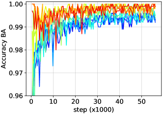
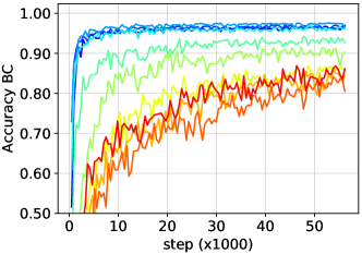
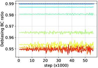
(a) Test accuracy (BA)	(b) Test accuracy (BC)	(c) Debiasing BC ratio

Figure 2: Learning curves of LW w.r.t. different training epochs of the biased classifier ($T_{\text{bias}}$), ranging from 2 to 80. The biased dataset is Colored MNIST with the BC ratio of 1%. The maximum sample weight is set to 100. Since BC samples account for 90% of the total test samples, the test accuracies for all samples are very similar to those for BC sample in (b).

We provide details for the optimizer, training epochs, learning rate, learning rate schedule, etc. corresponding to each dataset in Appdx. C.2.

5.2 Results when the bias label is available

Due to space constraint, we provide a detailed examination of our method’s performance in cases where the bias label is accessible in Appdx. D. To summarize, both WS and LW substantially outperform the vanilla classifier across Colored MNIST, Corrupted CIFAR10, and Biased CelebA, affirming the validity of our theoretical analysis in Section 3. Furthermore, our results indicate that LW consistently surpasses WS on the three datasets. Therefore, in the subsequent experiments, we will exclusively focus on LW.

5.3 Results when the bias label is unavailable

5.3.1 Results on Colored MNIST and Corrupted CIFAR10

As shown in Table 1, our proposed method LW significantly outperforms the vanilla classifier trained with the standard cross-entropy loss, as well as several other debiasing baselines such as ReBias [5], DFA [37], and SelecMix [24]. Furthermore, LW achieves higher test accuracies than LfF in most settings of Colored MNIST and Corrupted CIFAR10. Compared to the current state-of-the-art debiasing method PGD, LW performs slightly worse on Colored MNIST but demonstrates superior performance on Corrupted CIFAR10. Specifically, LW achieves about 1%, 4%, and 7% higher accuracy than PGD on Corrupted CIFAR10 with BC ratios of 0.5%, 1%, and 5%, respectively. Detailed comparisons between our method and LfF and PGD are provided in Appds. F.2 and F.1, respectively. These outcomes substantiate the efficacy of using the GCE loss to train a model of $p(y|x)$ that approximates $p(y|b)$, and endorse the practice of weighting each sample with $\frac{1}{p(y|b)}$ in our method.

5.3.2 Results on Biased CelebA and BAR

In this experiment, we only choose LfF and PGD as our baselines since the two methods have demonstrated superior performances compared to other approaches in our previous experiment and also in [3]. From Table 2, it is clear that LW outperforms LfF and PGD significantly on both Biased CelebA and BAR. Surprisingly, our experiments have revealed that in certain settings, LfF and PGD may perform even worse than the vanilla classifier, particularly on Biased CelebA with BC ratios of 1% and 5%. Additionally, we have noticed that LfF and PGD exhibit sensitivity to hyperparameters on Biased CelebA, as evidenced by the large standard deviations in their results. These findings raise concerns about the effectiveness of the debiasing formulas employed by LfF and PGD, which rely heavily on heuristics.

It is worth noting that on BAR, our implementation of the vanilla classifier achieves a higher test accuracy than what has been reported in [46] and [3]. This implies that the improvement of LW over the vanilla classifier on BAR can be attributed to its debiasing capability rather than the under-performance of the vanilla classifier. As far as we know, the result of LW on BAR presented in Table 2 currently represents the state-of-the-art performance in this domain.

5.4 Ablation Study

In this section, we closely examine two key hyperparameters that mainly influence the performance of our proposed LW. They are the number of training epochs for the biased classifier ($T_{\text{bias}}$), and the maximum sample weight ($\gamma$).

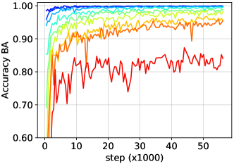
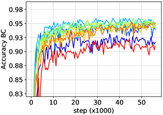
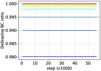
(a) Test accuracy (BA)	(b) Test accuracy (BC)	(c) Debiasing BC ratio

Figure 3: Learning curves of LW w.r.t. different values of the maximum sample weight ($\gamma$), ranging from 50 to $10^{6}$. The biased dataset is Colored MNIST with the BC ratio of 0.5%. The biased classifier is trained for 10 epochs. Since BC samples account for 90% of the total test samples, the test accuracies for all samples are very similar to those for BC sample in (b).

5.4.1 Effect of the number of training epochs for the biased classifier

Since the primary role of the biased classifier in LW is to capture solely the bias attribute $b$ in the input $x$, it is critical that the biased classifier should not be trained for too long. Otherwise, this classifier may capture the class attribute $u$, leading to an inaccurate approximation of $p(y|b)$ by $p_{\psi}(y|x)$. To validate this intuition, we compare the performances of various versions of LW in Fig. 5.1.3, each utilizing a biased classifier trained for different numbers of epochs $T_{\text{bias}}$. Apparently, as $T_{\text{bias}}$ decreases, LW achieves higher test accuracies on BC samples (Fig. 5.1.3b), indicating that $p_{\psi}(y|x)$ becomes a more reliable approximation of $p(y|b)$. However, if $T_{\text{bias}}$ is too small (e.g., $T_{\text{bias}}$ < 10), the biased classifier may not have undergone sufficient training to produce accurate class predictions, potentially hurting LW’s performance. In fact, the choice of $T_{\text{bias}}$ hinges on the learning capability of the biased classifier, which is examined in the appendix. Further empirical results of $T_{\text{bias}}$ can be found in the appendix.

It is worth noting that there is a strong correlation between the high test accuracy of LW and the proximity of its “debiasing BC ratio” $\beta$ to the ground-truth BA ratio (Fig. 5.1.3c). The debiasing BC ratio is computed by dividing the average loss weight over BC samples by the sum of the average loss weight over BC samples and the average loss weight over BA samples. Mathematically, $\beta=\frac{\mathbb{E}_{n\in\text{BC}}[w_{n}]}{\mathbb{E}_{n\in\text{BC}}[w_{n}]+\mathbb{E}_{n\in\text{BA}}[w_{n}]}$. Interestingly, in this particular setting, LW attains the highest test accuracy when its debiasing BC ratio coincides with the ground-truth BA ratio, which is 0.99. This remarkable alignment further corroborates our theoretical analysis, and demonstrates that the hidden true bias term $p(y|b)$ can be effectively approximated via a biased classifier trained with a limited number of epochs.

5.4.2 Effect of the maximum sample weight

The optimal value of the maximum sample weight $\gamma$ plays a crucial role in ensuring the proper normalization of sample weights $w_{n}$ and achieving a closer match with the true debiasing terms $\frac{1}{p(y_{n}|b_{n})}$. Generally, the choice of $\gamma$ depends primarily on the bias ratio present in the training data. To illustrate this, let’s consider the Colored MNIST dataset with a BA ratio of 0.995 and a BC ratio of 0.005. In this scenario, we would expect that BC samples are weighted approximately 200 times more than BA samples to achieve full debiasing (since $\frac{0.995}{0.005}$ $\approx$ 200). This implies that if BA samples have a weight of 1, BC samples should have a weight of 200. Assuming we have a perfect biased classifier which assigns a class confidence of 1 to BA samples and very low class confidences to BC samples (i.e., $p_{\psi}(y|x)$ $\approx$ 1 for BA samples and small for BC samples), we can compute the weights for BA samples as 1 and for BC samples as very large weights, which are then clamped at $\gamma$. By setting $\gamma$ to 200, we obtain the appropriate weights for BC samples, allowing for full debiasing as discussed earlier. Empirical validation of this reasoning is presented in Fig. 5.4b, where LW achieves the highest test accuracy on BC samples when $\gamma$ is equal to 200. Moreover, at this specific value of $\gamma$, the debiasing BC ratio of LW aligns with the ground-truth BA ratio of 0.995 (Fig. 5.4c), indicating that LW likely achieves full debiasing. However, it should be noted that when the bias classifier is not perfect, the optimal value of $\gamma$ would be different from the ground-truth $\frac{\text{BA ratio}}{\text{BC ratio}}$. Typically, a larger value of $\gamma$ would be used to assign more weight to BC samples predicted with high class confidences by the imperfect biased classifier. Regarding the test accuracy on BA samples, it monotonically decreases as $\gamma$ increases due to the widening gap between the weights of BC samples and BA samples (Fig. 5.4a). For more results of $\gamma$ on other datasets, please refer to the appendix.

6 Conclusion

We have proposed a novel method for mitigating dataset bias and analyzed our method from statistical and causal perspectives. While our approach yields promising results, certain limitations persist: i) our method depends on the training epochs of the biased classifier ($T_{\text{bias}}$) and the clamp threshold ($\gamma$) to produce good approximations of $p(y|b)$, which are hard to control in practice due to the variability introduced by the unknown bias rate; and ii) our method mitigates bias via balancing the sampling distribution during learning rather than directly adjusting the target. Nevertheless, these limitations are not unique to our method and are shared by other debiasing techniques. For instance, PGD’s dependence on $T_{\text{bias}}$ is also evident (in the appendix). Additionally, both PGD and LfF employ indirect bias mitigation like ours. In forthcoming work, we aim to develop a novel method to address the aforementioned limitations.

Table of Content for Appendix

1. 1 Introduction
2. 2 A Statistical View of Dataset Bias
3. 3 Mitigating Dataset Bias from Statistical and Causal Perspectives
   1. 3.1 Bias mitigation based on $p(u|b)$
   2. 3.2 Interpretation of $\mathcal{L}_{\theta}^{\text{LW}}$ from a causal perspective
   3. 3.3 Bias mitigation based on $p(b|u)$
4. 4 Related Work
5. 5 Experiments
   1. 5.1 Experimental Setup
      1. 5.1.1 Datasets
      2. 5.1.2 Baselines
      3. 5.1.3 Implementation details
         1. 5.2 Results when the bias label is available
            1. 5.3 Results when the bias label is unavailable
               1. 5.3.1 Results on Colored MNIST and Corrupted CIFAR10
               2. 5.3.2 Results on Biased CelebA and BAR
                  1. 5.4 Ablation Study
                     1. 5.4.1 Effect of the number of training epochs for the biased classifier
                        1. 5.4.2 Effect of the maximum sample weight
                           1. 6 Conclusion
                              1. A More discussion about related work
                              2. B Technical comparisons between LfF, PGD and our method
                              3. C Further details about datasets and training settings
                                 1. C.1 Datasets
                                 2. C.2 Optimization hyperparameters
                                 3. C.3 Data augmentation
                                 4. C.4 Optimal settings of our method
                              4. D Results when the bias label is available
                                 1. E Additional ablation study results for LW
                                    1. F Additional experimental results
                                       1. F.1 Additional results of LfF in comparison with LW
                                          1. F.2 Additional results of PGD in comparison with LW
                                             1. F.3 Analysis of the Biased Classifier
                                                1. F.4 Target Bias Adjustment - an extension of BiasBal to deal with unknown bias
                                                   1. G Bias mitigation based on $p(b|u)$
                                                      1. G.1 Idea
                                                      2. G.2 Using $p_{\varphi}(y|z)$ instead of $p_{\varphi}(z|y)$
                                                         1. G.3 Derivations of the lower bounds of $\log p_{\theta,\varphi}(x|y)$ and $\log q_{\varphi,\phi}(y|x)$

Appendix A More discussion about related work

Early works on dataset bias mitigation

The presence of bias in the training data has long been recognized and acknowledged due to its negative impacts on the generalizability of practical machine learning systems. Earlier works, such as [28, 56] mention “dataset bias” and view it as the phenomenon where a model performs well on one dataset but poorly on others. They provide some explanations for this phenomenon, such as, bias may come from the process of data selection, capturing, or labeling [56]. They also propose a simple solution to reduce bias by learning an SVM on multiple datasets, with additional regularization on the weights that capture various forms of bias across those datasets [28]. Later, Alvi et al. [4] introduce a debiased method that also leverages multiple datasets. Their model has a deep convolutional neural network backbone for feature extraction, a primary head for the main task, and multiple secondary heads for capturing spurious variations or biases present in the datasets. By minimizing the classification loss w.r.t. the primary head and the (bias) confusion loss w.r.t. the secondary heads, their model could learn features that are useful for the main task but invariant to the spurious variations. In another study, Li et al. [40] examine a different type of bias referred to as “representation bias”, and contrast it with the dataset bias in [28]. To put it simply, representation bias arises when a model is trained on datasets that favor certain representations over others. Consequently, the model tends to rely on these biased representations to solve the task, limiting its ability to generalize beyond the training datasets. This bias is closely related to the feature-correlation bias considered in our paper. Li et al. [40] also introduce a method to quantify representation bias by analyzing the classifier’s performance. In their subsequent work [39], they define representation bias as the normalized mutual information between the feature vector and the class label, and proposed a debiasing method that optimizes the classifier’s parameters and the sample weights in an adversarial manner.

Group-DRO-based Methods

Group DRO [23, 53] is a variant of DRO [6, 13], which aims to train a robust (against group shifts) classifier by minimizing the worst-case expected loss over a set of distributions $Q$ defined as a mixture of sample groups. There are various ways to characterize a group. In the context of bias mitigation, a group is typically associated with a pair of class and bias attributes $(u,b)$ [42, 53]. When $u$, and $b$ are known and discrete, a group $(u,b)$ can be explicitly identified. Sagawa et al. [53] discovered that naively applying group DRO to train overparameterized neural networks does not enhance performance on the test worst group compared to the standard empirical risk minimization (ERM). To address this, they propose imposing stronger regularizations, such as L2 penalty or early stopping, on the group DRO model to improve generalization and achieve better worst-group accuracies in testing. Liu et al. [42] introduce Just Train Twice (JTT), a two-stage approach, that does not require group annotation during training. In the first stage, this method trains a classifier with ERM for some epochs on the original training data, and constructs an error set comprising samples misclassified by the classifier. In the second stage, it trains another “robust” classifier with samples in the error set upweighted by a constant value $\lambda>1$. The rationale is that samples in the error set likely originate from challenging groups (i.e., groups corresponding to bias-conflicting samples), and assigning them higher weights encourages the classifier to focus more on these groups. Correct-N-Contrast (CnC) [63] is an extension of JTT, also involving two training stages. The first stage of CnC resembles that of JTT, entailing training an ERM classifier. The second stage incorporates contrastive learning with the anchor, positives, and negatives selected based on the class label and ERM prediction.

Class Imbalance Bias Mitigation

A closely related type of bias that also arises in our formula in Eq. 4 is class imbalance [7, 9, 12, 10, 18, 26, 33, 34, 41]. When the classes are not evenly distributed, the model is prone to predicting the more common classes. Compared to feature-correlation bias, this bias is more apparent and has been studied for a longer period of time. Popular methods for mitigating class imbalance bias include resampling [7, 10, 15], and cost-sensitive learning [9, 12, 14, 27, 33]. Resampling aims to balance the class prior by either oversampling a minor class $y$ at a rate of $\frac{p(y_{\text{most}})}{p(y)}$ or undersampling a major class $y$ at a rate of $\frac{p(y_{\text{least}})}{p(y)}$, depending on whether the reference is the most class $y_{\text{most}}$ or the least class $y_{\text{least}}$. In mini-batch learning via random sampling with replacement, the two resampling strategies are the same. An inherent limitation of resampling is that samples of the minor class are duplicated, which can lead to overfitting [18]. To address this problem, different variants of resampling have been proposed [18]. One notable technique is Synthetic Minority Oversampling TEchnique (SMOTE) [10], which generates synthetic samples of the minor class for oversampling by combining the feature vector of a sample of interest with its nearest neighbor feature vector through interpolation, similar to latent mixup [58] and SelecMix [24]. In cost-sensitive learning, higher losses are assigned to samples belonging to the minor class to account for their lower frequency. This can be achieved by either reweighting the loss function by a scalar (e.g., the inverse class frequency) or by designing new losses that inherently incorporate the sample weight [9, 12, 27, 41]. In general, addressing the class imbalance bias is easier than addressing the feature-correlation bias, as the former does not involve the bias attribute.

Causal Inference

In the realm of causal inference, bias typically arises as a non-causal (spurious) association between the treatment and target variables mediated by a confounder. This bias is commonly known as “confounding bias”. Causal inference offers useful techniques and methodologies for mitigating such bias, with inverse probability weighting (IPW) [20, 21] being one of them. Other approaches include causal invariant representation learning [44, 45, 60], proxy variables [62], front-door adjustment [47], which have been studied recently for various generalization tasks.

Appendix B Technical comparisons between LfF, PGD and our method

Below, we provide a technical comparisons between LfF, PGD and our method.

LfF [46] is a reweighting method like our LW, which trains a biased classifier $p_{\psi}(y|x)$ and a debiased classifier $p_{\theta}(y|x)$ in parallel. The weight for each sample $n$ is computed as follows:

$$w_{n} =\frac{\mathcal{L}_{\psi}^{\text{xent}}(x_{n},y_{n})}{\mathcal{L}_{\psi}^{\text{xent}}(x_{n},y_{n})+\mathcal{L}_{\theta}^{\text{xent}}(x_{n},y_{n})}$$ (19)

$$=\frac{1}{1+\frac{\mathcal{L}_{\theta}^{\text{xent}}(x_{n},y_{n})}{\mathcal{L}_{\psi}^{\text{xent}}(x_{n},y_{n})}}=\frac{1}{1+\frac{-\log p_{\theta}(y_{n}|x_{n})}{-\log p_{\psi}(y_{n}|x_{n})}}$$ (20)

where $\mathcal{L}_{\psi}^{\text{xent}}(x_{n},y_{n})$ and $\mathcal{L}_{\theta}^{\text{xent}}(x_{n},y_{n})$ are the losses of the biased and debiased classifiers, respectively. Since $\mathcal{L}_{\psi}^{\text{xent}}(x_{n},y_{n})$ and $\mathcal{L}_{\theta}^{\text{xent}}(x_{n},y_{n})$ are non-negative, $w_{n}\in[0,1]$, which ensures stability during training of the debiased classifier. Moreover, the weight in Eq. 20 exhibits a time-varying behavior similar to ALW. At the initial stages of training, when both the biased and debiased classifiers have limited learning, $\mathcal{L}_{\psi}^{\text{xent}}(x_{n},y_{n})$ and $\mathcal{L}_{\theta}^{\text{xent}}(x_{n},y_{n})$ have large values and are roughly the same. Consequently, the weights for all training samples are approximately equal, around 0.5. This enables the debiased classifier to learn from all samples effectively in the early stages. As the training progresses, $\mathcal{L}_{\psi}^{\text{xent}}(x_{n},y_{n})$ tends to decrease for BA samples and increase (or decrease at a much slower rate) for BC samples (Fig. F.3). As a result, the weights for BA and BC samples gradually become smaller and larger, respectively, encouraging the debiased classifier to focus less on BA samples and more on BC samples.

PGD [3] is a two-stage resampling method like our WS. In the first stage, it trains a biased classifier $p_{\psi}(y|x)$ using the GCE loss to distinguish between BC and BA samples. In the second stage, it calculates the resampling weight $w_{n}$ for each training sample $n$ as the normalized L2 norm of the gradient of $\mathcal{L}_{\psi}^{\text{xent}}(x_{n},y_{n})$ w.r.t. the parameters of the final fully-connected (FC) layer of the biased classifier. The computation of $w_{n}$ is given by:

$$w_{n}=\frac{\left\|\nabla_{\psi_{\text{top}}}\mathcal{L}_{\psi}^{\text{xent}}(x_{n},y_{n})\right\|_{2}}{\sum_{(x_{m},y_{m})\in\mathcal{D}}\left\|\nabla_{\psi_{\text{top}}}\mathcal{L}_{\psi}^{\text{xent}}(x_{m},y_{m})\right\|_{2}}$$ (21)

Since $w_{n}$ is used for resampling instead of reweighting, we can safely ignore the denominator in the above formula of $w_{n}$ and consider $w_{n}=\left\|\nabla_{\psi_{\text{top}}}\mathcal{L}_{\psi}^{\text{xent}}(x_{n},y_{n})\right\|_{2}$. It is worth noting that the final layer’s output is the class probability vector $p_{n}$ computed as $p_{n}$ = $p_{\psi}(Y|x_{n})$ = $\text{softmax}\left(\mathrm{W}^{\top}h_{n}+\mathrm{b}\right)$ where $h_{n}$, $\mathrm{W}$, and $\mathrm{b}$ represent the input, weight and bias of the final layer, respectively. Therefore, we can compute $w_{n}$ as follows $w_{n}$ = $\left\|\nabla_{\mathrm{W}}\left(-\log p_{\psi}(y_{n}|x_{n})\right)\right\|_{2}$ = $\left\|\left(p_{n}-1_{y_{n}}\right)h_{n}^{\top}\right\|_{2}$ with $1_{y_{n}}$ representing the one-hot vector at $y=y_{n}$. For BA samples, $w_{n}$ tends to be 0 since $p_{n}\approx 1_{y_{n}}$ and $\nabla_{\mathrm{W}}\mathcal{L}_{\psi}^{\text{xent}}(x_{n},y_{n})\approx 0$. This implies that BA samples may hardly contribute to training the debiased classifier, which can results in the inferior performance of PGD in some cases.

Appendix C Further details about datasets and training settings

C.1 Datasets

We provide summarization of the datasets used in our experiment in Table 3.

Dataset	Image size	Target	Bias	#classes
Colored MNIST	3$\times$32$\times$32	Digit	BG Color	10
Corrupted CIFAR10	3$\times$32$\times$32	Object	Noise	10
Biased CelebA	3$\times$128$\times$128	Hair color	Gender	2
BAR	3$\times$256$\times$256	Action	Context	6

Table 3: Summarization of the datasets used in our experiments

C.2 Optimization hyperparameters

We provide the optimization hyperparameters for our method in Table 4.

Dataset	$opt$	$lr$	$wd$	$mo$	$ld$	$ldep$	$ep$	$bs$
Colored MNIST	Adam	1e-3	-	-	-	-	120	128
Corrupted CIFAR10	Adam	1e-3	-	-	-	-	160	128
Biased CelebA	SGD	1e-3	1e-4	0.9	0.1	80, 120	160	256
BAR	SGD	1e-3	1e-5	0.9	0.1	80, 120	160	128

Table 4: Optimization hyperparameters for our method across different datasets. Abbreviation meanings: $opt$ (optimizer), $lr$ (learning rate), $wd$ (weight decay), $mo$ (momentum), $ld$ (learning rate decay), $ldep$ (epochs at which learning rate are decayed), $ep$ (total number of epochs), $bs$ (batch size).

C.3 Data augmentation

For Colored MNIST, we do not use any data augmentation. For Corrupted CIFAR10, we use RandomCrop(32, padding=4) followed by RandomHorizontalFlip(). For Biased CelebA, we resize the input image to the specified size, and use RandomHorizonalFlip(). For BAR, we use RandomResizedCrop(256, scale=(0.3, 1.0)) followed by RandomHorizontalFlip().

C.4 Optimal settings of our method

In Table 5, we provide the optimal settings of our proposed method LW.

Dataset	BC (%)	Biased Classifier	LW
		$T_{\text{bias}}$	$\gamma$	$T_{\text{anneal}}$
Colored MNIST	0.5	10	200	0
	1.0	10	100
	5.0	1$\rightarrow$2	20
Corrupted CIFAR10	0.5	100$\rightarrow$160	2k$\rightarrow$5k	40
	1.0	60$\rightarrow$160	1k$\rightarrow$5k
	5.0	20	500$\rightarrow$5k
Biased CelebA	0.5	160	500	0
	1.0	160	500
	5.0	160	500
BAR	-	10	50$\rightarrow$100	0

Table 5: Optimal settings of our method.

Appendix D Results when the bias label is available

Dataset	BC (%)	Vanilla	LNL	BiasBal	WS	LW
Colored MNIST	0.5	80.18$\pm$1.38	80.05$\pm$1.02	97.44$\pm$0.12	96.15$\pm$0.33	96.16$\pm$0.35
	1.0	87.48$\pm$1.75	87.52$\pm$1.53	97.89$\pm$0.20	97.58$\pm$0.09	97.11$\pm$0.12
	5.0	97.04$\pm$0.21	98.77$\pm$0.18	98.92$\pm$0.13	98.92$\pm$0.07	98.55$\pm$0.07
Corrupted CIFAR10	0.5	28.00$\pm$1.15	28.13$\pm$0.98	45.52$\pm$1.37	31.02$\pm$0.72	36.50$\pm$0.51
	1.0	34.56$\pm$0.87	34.43$\pm$1.03	53.18$\pm$1.87	40.06$\pm$1.24	46.41$\pm$1.46
	5.0	59.33$\pm$1.26	59.52$\pm$0.85	72.60$\pm$0.69	69.91$\pm$0.54	70.29$\pm$0.75
Biased CelebA	0.5	77.43$\pm$0.42	76.64$\pm$0.73	87.74$\pm$0.19	78.48$\pm$0.62	86.49$\pm$0.33
	1.0	80.58$\pm$0.41	79.72$\pm$0.54	87.82$\pm$0.36	82.41$\pm$0.33	85.32$\pm$0.40
	5.0	86.35$\pm$0.33	86.41$\pm$0.35	88.78$\pm$0.22	86.90$\pm$0.23	87.83$\pm$0.21

Table 6: Results of different debiasing methods when the bias label is available. The best and second best results are highlighted in bold and gray, respectively.

	Colored MNIST	Corrupted CIFAR10	Biased CelebA
Test Acc.
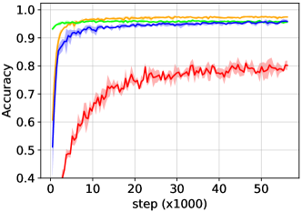
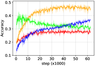
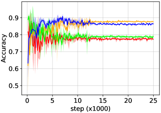
Test Xent

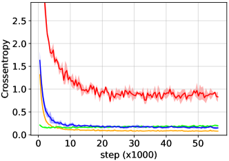
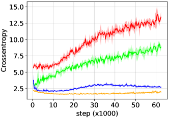
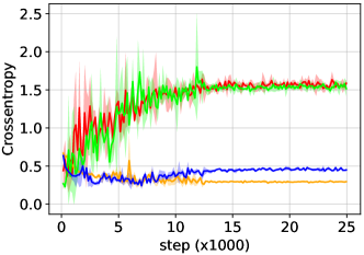
Figure 4: Test curves of the vanilla classifier, BiasBal, and our proposed methods WS and LW on Colored MNIST, Corrupted CIFAR10, and Biased CelebA with the BC ratio of 0.5%. The bias label is assumed to be given, and $p(y|b)$ used in BiasBal, WS, and LW is estimated directly from training data.

In this section, we aim to empirically validate our theoretical analysis on feature-correlation bias in Sections 2 and 3 by examining the effectiveness of our proposed weighted sampling (WS) and loss weighting (LW) techniques in mitigating bias in datasets with known discrete bias labels. We consider Learning Not to Learn (LNL) [29] and Bias Balancing (BiasBal) [22] as baselines since these approaches explicitly utilize the bias label. From Table D, it is evident that classifiers trained with either WS or LW achieve significantly higher test accuracies than the vanilla classifier. This observation suggests that WS and LW effectively reduce bias in training data, validating our theoretical analysis. However, WS and LW exhibit distinct training dynamics, resulting in varying levels of effectiveness in bias mitigation. As depicted in Fig. D, on Corrupted CIFAR10, WS quickly achieves good performance in the early stages of training but gradually degrades over time. We hypothesize that this behavior is attributed to the lack of data diversity resulting from over/under-sampling of BC/BA samples in WS. On the other hand, LW takes more time than WS to achieve similar performance due to its small updates on most training samples (i.e., BA samples). Nonetheless, LW demonstrates a steady improvement in performance.

Besides, WS and LW outperform LNL, a method that aims to learn features independent of bias information. Interestingly, during our experiments, we observed minimal performance difference between LNL and the vanilla classifier, as shown in Table D. This suggests that the features learned by LNL still contain bias information. We hypothesize that when class and bias labels are highly correlated, it becomes challenging from a statistical perspective to learn features that are truly independent of bias while accurately predicting the class.

However, our methods perform worse and are less robust than BiasBal, especially on Corrupted CIFAR10. Fig. D illustrates that BiasBal converges more rapidly than our methods with higher test accuracies and smaller test crossentropy losses in most settings. The exceptional performance of BiasBal motivates us to delve deeper into the theoretical mechanisms and design differences between BiasBal and our methods that account for BiasBal’s superior performance.

We discovered that like LW, BiasBal mitigates bias via reweighting the model trained on biased data. It also arrives at the same reweighting term of $\frac{1}{p(y|b)}$ as in LW despite employing a different reasoning technique that leverages Bayes’ rule and two assumptions: i) $p(y|x)=p(y|x,b)$ and ii) $p(x|y,b)$ are the same across different joint distributions $p(y,b)$. The bias correction formula of BiasBal (Eq. A.8 in the supplementary material of [22]) is given as follows:

$$p_{train}(y|x)=p_{u}(y|x)p_{train}(y|b)\frac{K}{C}$$ (22)

where $p_{train}$ and $p_{u}$ denotes the distribution over the biased training data and the unbiased distribution in which $y$ and b are independent, respectively; $C$ is the number of classes, and $K=\frac{p_{u}(x|b)}{p_{train}(x|b)}$ is a constant w.r.t. $y$. Eq. 22 implies that $p_{u}(y|x)$ $\propto$ $p_{train}(y|x)\frac{1}{p_{train}(y|b)}$, allowing us to reweight the biased distribution $p_{train}(y|x)$ by $\frac{1}{p_{train}(y|b)}$ to achieve a theoretically unbiased distribution.

The key distinction between BiasBal and WS/LW lies in their respective debiasing mechanisms. While WS/LW corrects the learning process of $p_{\theta}(y|x)$ (via resampling/reweighting the training data distribution) to achieve an unbiased target $p_{\theta}(y|x)$ indirectly, BiasBal directly corrects the target $p_{\theta}(y|x)$ and learns with the (unnormalized) bias-adjusted target $\hat{p}_{\theta}(y|x)=p_{\theta}(y|x)p_{train}(y|b)$. This debiasing mechanism of BiasBal is generally more robust than that of WS/LW, as it neither compromises the diversity of training data nor introduces training instability. Moreover, while WS and LW focus on correcting bias in $p(y_{n}|x_{n})$ for the class $y_{n}$ associated with a particular input $x_{n},$ BiasBal considers bias correction of $p(y|x_{n})$ for every class $y$. These advancements in the debiasing mechanism of BiasBal likely contribute to its superior performance.

It is worth noting that the original paper [22] on BiasBal exclusively applies the method when the bias label is discrete and known, as $p_{train}(y|b)$ can be estimated nonparametrically from the training data. However, with our proposed method for approximating $p_{train}(y|b)$ using the biased classifier, as discussed in Section 3.1, we can readily extend BiasBal to scenarios where the bias label is either unavailable or continuous. In Appdx. F.4, we provide a detailed analysis of this extended version of BiasBal, which we refer to as “Target Bias Adjustment” (TBA) to better describe its characteristic of adjusting the target distribution.

Appendix E Additional ablation study results for LW

We provide additional experiments examining the impact of varying the number of training epochs for the biased classifier and adjusting the maximum cutoff for sample weights on the performance of LW in Figs. E and E.

	Colored MNIST (5%)	Corrupted CIFAR10 (5%)
Test Acc.
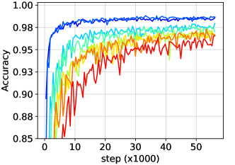
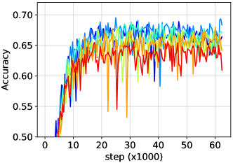
Test Acc. BA
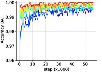
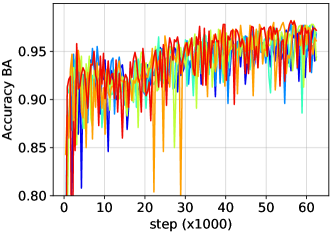
Test Acc. BC
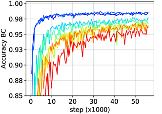
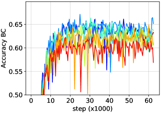
Debias. BC Ratio

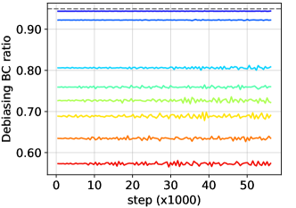
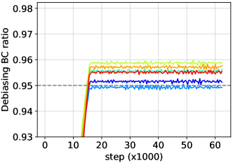
Figure 5: Learning curves of LW w.r.t. different training epochs of the biased classifier ($T_{\text{bias}}$) on Colored MNIST and Corrupted CIFAR10. Both datasets have the BC ratio of 5%. Maximum sample weights ($\gamma$) for the two datasets are set to 20 and 50, respectively.

	Colored MNIST (5%)	Corrupted CIFAR10 (0.5%)	Biased CelebA (0.5%)
Test Acc.
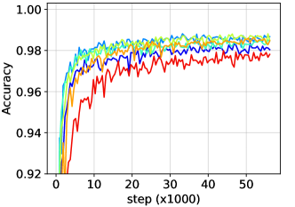
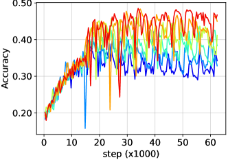
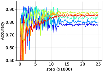
Test Acc. BA
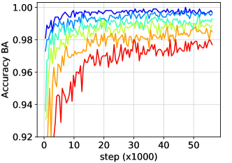
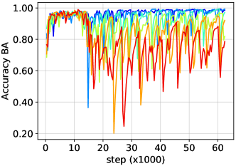
Test Acc. BC
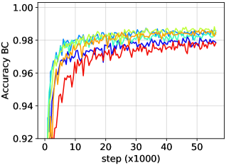
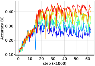
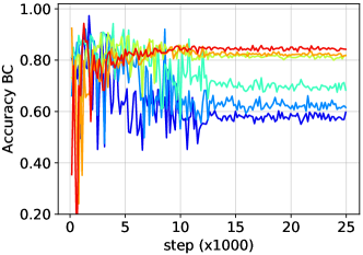
Debias. BC Ratio

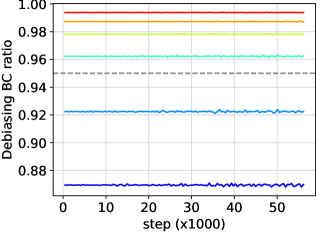
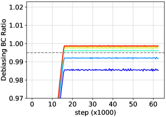
Figure 6: Learning curves of LW w.r.t. different values of $\gamma$ on Colored MNIST, Corrupted CIFAR10, and Biased CelebA. These datasets have respective BC ratios of 5%, 0.5%, and 0.5%. Biased classifiers for these datasets are trained for 2, 120, and 160 epochs, respectively.

Appendix F Additional experimental results

F.1 Additional results of LfF in comparison with LW

It can be seen from Table 1 that LfF, despite requiring minimal hyperparameter tuning, performs well on both Colored MNIST and Corrupted CIFAR10. Surprisingly, it even outperforms later proposed methods such as DFA, SelecMix on both Colored MNIST and Corrupted CIFAR10, as well as PGD on Corrupted CIFAR10. We hypothesize that there could be several possible reasons for this:

1. Some methods like PGD rely heavily on specific data augmentation techniques (e.g., color jitter) for optimal performance, which are not utilized in this work (Section 5.1.3).

2. The selected hyperparameters for DFA and SelecMix in this study may not be optimal since we reimplemented these methods ourselves and were unable to thoroughly explore every configuration due to time constraints.

3. It might be that in previous works, LfF unintentionally yields poor results, particularly on Colored MNIST, despite being implemented correctly.

Regarding the third point, we have found that the biased classifier often experiences sudden collapses during training if its architecture does not include Batch Norm [25] while the vanilla classifier does not exhibit this issue. Our hypothesis is that the GCE loss of the biased classifier is primarily optimized for frequently occurring BA samples. As a result, the loss surface surrounding sporadic BC samples becomes highly volatile, leading to substantial gradient updates (in the absence of Batch Norm) whenever these BC samples are encountered during training. This volatility causes the biased classifier’s parameters to collapse to irrecoverable states. We visualize this phenomenon of LfF in Fig. F.1, utilizing LeNet5 as the biased classifier architecture without any Batch Norm layer. It is evident that the cross-entropy loss of this classifier abruptly spikes to hundreds for both BC and BA samples at certain steps during training and fails to recover. This makes the relative difficulty scores of BA samples close to 1 (instead of being close to 0), resulting in a degradation of LfF’s test accuracy.

The reason why we raise the third point and carefully analyze is due to the varying results of LfF reported in different studies [3, 22, 24, 37]. Some works utilizing multilayer perceptrons (MLPs) as the architecture for the biased classifier only achieve test accuracies of 52.50% [37] and 63.86% [24] for LfF on Colored MNIST with a BC ratio of 0.5%, while others adopting convolutional networks with Batch Norm can achieve significantly higher test accuracies of 90.3% [22] and 91.35% [3].

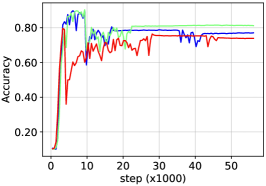
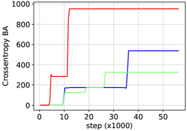
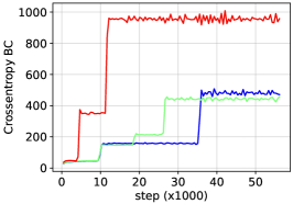
(a) Accuracy	(b) Cross-entropy BA	(c) Cross-entropy BC

Figure 7: Test results of 3 different runs of LfF [46] on Colored MNIST with a BC ratio of 0.5% where the classifier’s architecture is LeNet5 .

From Fig. F.1, we can clearly see that LfF achieves lower test accuracies than LW for both BA and BC samples on Colored MNIST. Furthermore, the test accuracy curves of LW exhibit a steady upward trend over time for both BA and BC samples. In contrast, the test accuracy curve for BA samples of LfF exhibits a decline followed by an increase, while the test accuracy curve for BC samples of LfF shows an increase followed by a decrease. This behavior aligns with the dynamics of the debiasing BC ratio of LfF (row 3 in Fig. F.1), which initially increases during the early stages of training and then decreases. This can be attributed to the fact that the biased classifier achieves a faster reduction in cross-entropy loss for BC samples compared to BA samples as the training progresses (rows 4, 5 in F.1), resulting in smaller sample weights for BC samples at a faster rate than those for BA samples. However, on Corrupted CIFAR10, the sample weights for BC samples decrease at a slower rate than those for BA samples, making the debiasing BC ratios of LfF increase over time (rows 4, 5 in F.1). A larger debiasing BC ratio often leads to higher test accuracy for BC samples since this kind of samples are assigned with larger weights during training.

	0.5%	1%	5%
Test Acc. BA
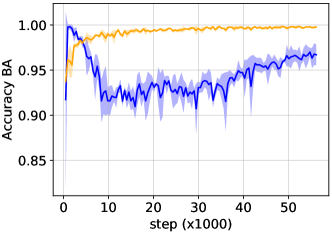
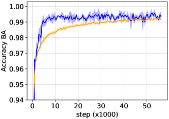
Test Acc. BC
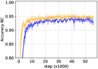
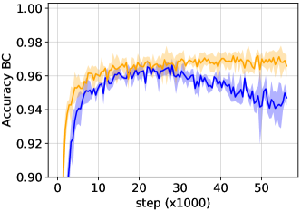
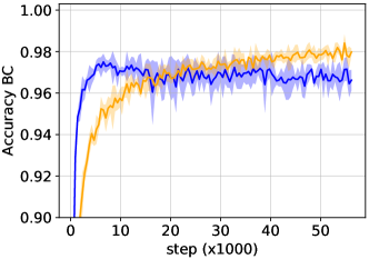
Debias. BC Ratio
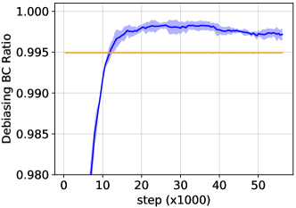
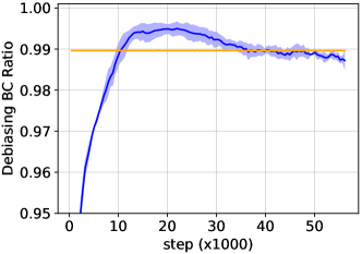
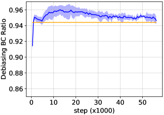
Sample Weight BA
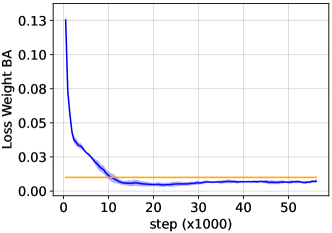
Sample Weight BC

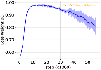
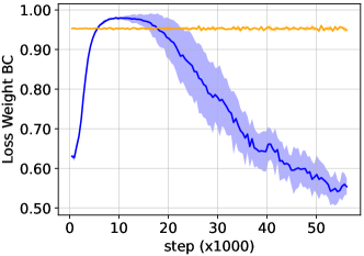
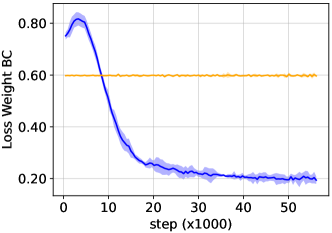
Figure 8: Learning curves of LfF and LW on Colored MNIST. The sample weights of LW, originally in the rage $\left[\frac{10}{\gamma},10\right]$, are scaled to the range $\left[\frac{1}{\gamma},1\right]$ to match the range [0, 1] of the sample weights of LfF.

	0.5%	1%	5%
Test Acc. BA
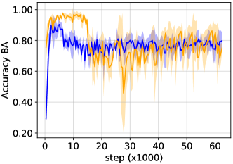
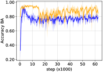
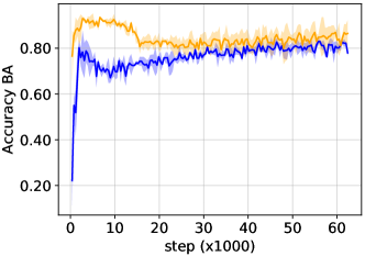
Test Acc. BC
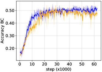
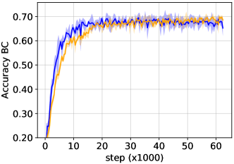
Debias. BC Ratio
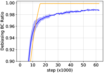
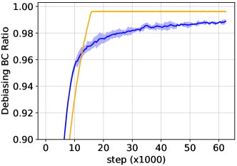
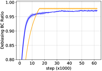
Sample Weight BA
Sample Weight BC

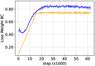
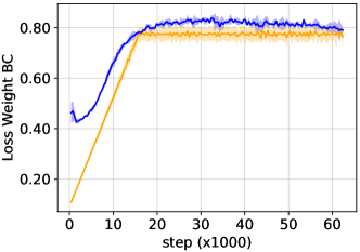
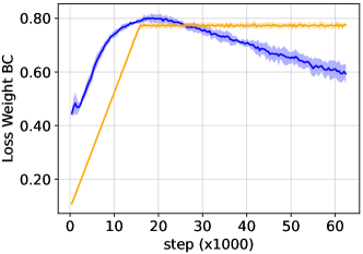
Figure 9: Learning curves of LfF and LW on Corrupted CIFAR10. The sample weights of LW, originally in the rage $\left[\frac{10}{\gamma},10\right]$, are scaled to the range $\left[\frac{1}{\gamma},1\right]$ to match the range [0, 1] of the sample weights of LfF.

F.2 Additional results of PGD in comparison with LW

From Fig. F.2, it is clear that PGD achieves the best test accuracies for both BA and BC samples on Colored MNIST when the biased classifier is trained for only one epoch. This holds true for different values of the BC ratio. However, on Corrupted CIFAR10, the best performance of PGD is obtained when the biased classifier is trained with a large number of epochs (can be up to hundreds) as shown in Fig. F.2. Such inconsistency makes the analysis and real-world application of PGD difficult. In almost all settings, we observe that PGD achieves higher cross-entropy losses than our method for both BA and BC samples, suggesting that the debiased classifier learned by PGD is less stable than the counterpart learned by our method. We hypothesize that it is because the debiased classifier of PGD is derived from the biased classifier, thus, may inherit the instability of the biased classifier.

	0.5%	1%	5%
Test Acc. BA
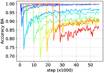
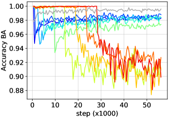
Test Acc. BC
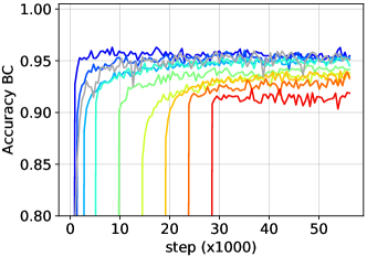
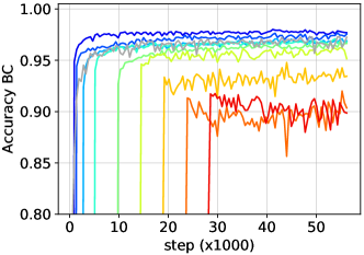
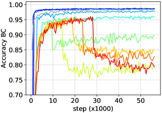
Test Xent BA
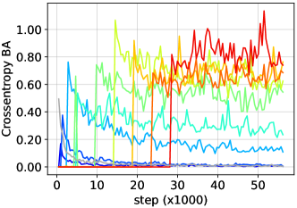
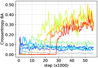
Test Xent BC

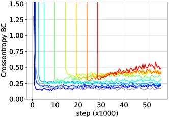
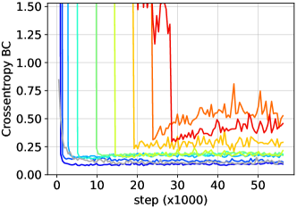
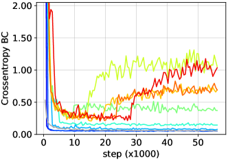
Figure 10: Learning curves of PGD on Colored MNIST by varying the number of training epochs for the biased classifier. The abrupt changes observed in the above figures indicate the transition from biased classifier training to debiased classifier training. We also show the learning curves of our proposed LW in gray for convenient comparison.

	0.5%	1%	5%
Test Acc. BA
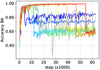
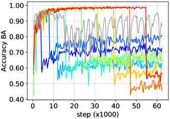
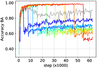
Test Acc. BC
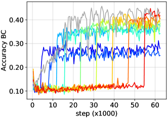
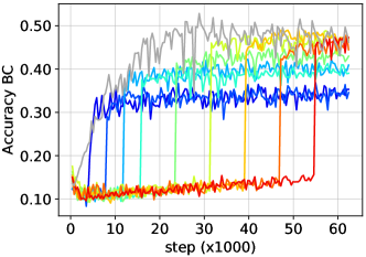
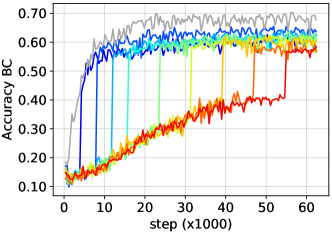
Test Xent BA
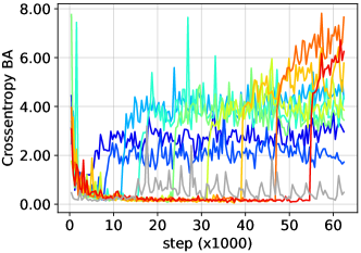
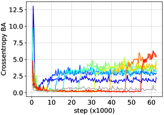
Test Xent BC

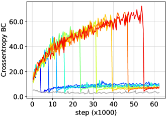
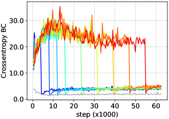
Figure 11: Learning curves of PGD on Corrupted CIFAR10 by varying the number of training epochs for the biased classifier. The abrupt changes observed in the above figures indicate the transition from biased classifier training to debiased classifier training. We also show the learning curves of our proposed LW in gray for convenient comparison.

F.3 Analysis of the Biased Classifier

In Fig. F.3, we show the learning curves of the biased classifier $p_{\psi}(y|x)$ trained on Colored MNIST, Corrupted CIFAR10, and Biased CelebA, considering various BC ratios. Apparently, the biased classifier exhibits higher test accuracy with prolonged training, indicating the necessity of employing an early stopping strategy in some cases to prevent the biased classifier from learning class semantics. For example, on Colored MNIST with a BC ratio of 5%, the biased classifier can achieve about 90% test accuracy after just 10 training epochs. Therefore, for Colored MNIST with a BC ratio of 5%, we need to set the training epoch of the biased classifier to 1 to ensure that $p_{\psi}(y|x)$ is a good approximation of $p_{\psi}(y|b)$ as shown in Table 5. On Corrupted CIFAR10 with BC ratios of 0.5% and 1%, the test accuracy of the biased classifier does not show significant improvement even when trained until the final epoch (160). This clarifies why, in Table 5, the optimal number of training epochs for the biased classifier in these settings falls within a range rather than being a specific value.

Another interesting thing that can be seen from Fig. F.3 is the positive correlation between the training accuracy and cross-entropy curves for BC samples on Corrupted CIFAR10, Biased CelebA, and Colored MNIST, while normally the two curves should be contradictory. Our conjecture is that although more BC samples are classified correctly by the biased classifier, those that are misclassified are assigned low probabilities. Because the GCE loss encourages the biased classifier to ignore samples with low probabilities, the probabilities of the misclassified samples decrease gradually during training, resulting in an increase in the cross-entropy loss. It should be noted that even a single sample misclassified with a probability of zero can lead to an extremely high cross-entropy loss, as the negative logarithm of zero approaches infinity ($-\log 0$ $\approx$ $\infty$). This finding provides a better explanation for our observation about the biased classifier’s collapse during training discussed in Section F.1.

	Colored MNIST	Corrupted CIFAR10	Biased CelebA
Test Acc. BA
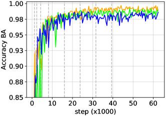
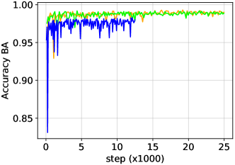
Test Acc. BC
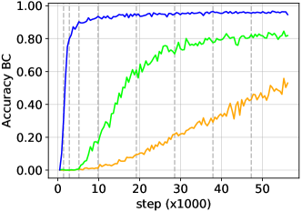
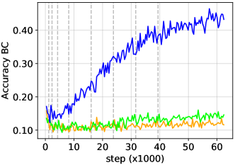
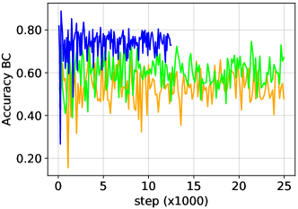
Train Acc. BA
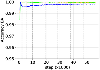
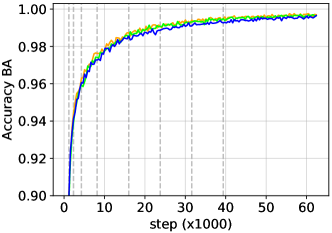
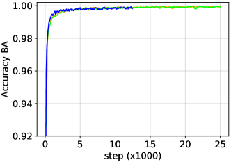
Train Acc. BC
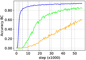
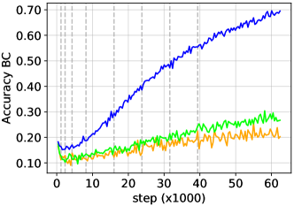
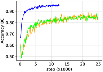
Train Xent BA
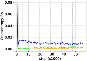
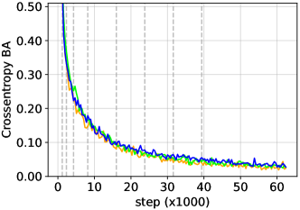
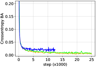
Train Xent BC

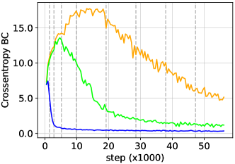
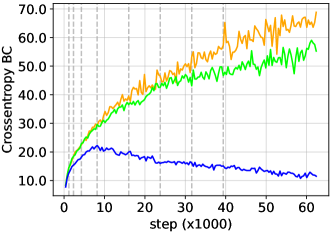
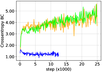
Figure 12: Learning curves of the biased classifier trained on Colored MNIST, Corrupted CIFAR10, and Biased CelebA with varying BC ratios of 0.5%, 1%, 2%, and 5%. The dashed lines in each plot, arranged from left to right, indicate the training epochs of 2, 5, 10, 20, 40, 60, 80, and 100.

F.4 Target Bias Adjustment - an extension of BiasBal to deal with unknown bias

Recalling that BiasBal [22] incorporates the bias in training data into its classifier via the following adjustment formula:

$$\tilde{p}_{\theta}(y|x)=p_{\theta}(y|x)p(y|b)$$

where $p_{\theta}(y|x)$ and $\tilde{p}_{\theta}(y|x)$ are the original and adjusted outputs of the classifier, respectively. However, since $\tilde{p}_{\theta}(y|x)$ is unnormalized under this adjustment formula (i.e., $\sum_{c=1}^{C}\tilde{p}_{\theta}(y=c|x)\neq 1$), we can rewrite $\tilde{p}_{\theta}(y|x)$ in its normalized form as follows:

$$\tilde{p}_{\theta}(y=c|x)=\frac{\exp\left(f_{\theta}(x)[c]+\log p(y=c|b)\right)}{\sum_{k=1}^{C}\exp\left(f_{\theta}(x)[k]+\log p(y=k|b)\right)}$$

If we assume $p_{\theta}(y|x)$ to be an unbiased prediction, $\tilde{p}_{\theta}(y|x)$ will be the biased prediction associated with the bias in training data. Therefore, to learn an unbiased classifier $p_{\theta}(y|x)$ given a biased training dataset, BiasBal maximizes the log-likelihood of $\tilde{p}_{\theta}(y|x)$ (instead of $p_{\theta}(y|x)$) over the training data. Its training loss is given below:

$$\mathcal{L}_{\theta}^{\text{BiasBal}}:=\mathbb{E}_{p_{\mathcal{D}}(x_{n},y_{n})}\left[-\log\tilde{p}_{\theta}(y_{n}|x_{n})\right]$$

Originally designed for discrete bias labels, BiasBal depended on the direct estimation of $p(y|b)$ from training data. To expand its applicability to unknown or continuous bias labels, we propose approximating $p(y|b)$ using the technique detailed in Section 3.1. This involves training a biased classifier $p_{\psi}(y|x)$ with a bias amplification loss, viewing it as an approximation of as an approximation of $p(y|b)$. To ensure stability in computing $\tilde{p}_{\theta}(y|x)$, $p_{\psi}(y|x)$ is clamped to values greater than $\frac{1}{\gamma}$, where $\gamma>0$ (as in Eq. 6). This results in:

$$\tilde{p}_{\theta}(y=c|x)=\frac{\exp\left(f_{\theta}(x)[c]+\log v[c]\right)}{\sum_{k=1}^{C}\exp\left(f_{\theta}(x)[k]+\log v[k]\right)}$$

where $v=\max\left(p_{\psi}(y|x),\frac{1}{\gamma}\right)$. We call this extension of BiasBal “Target Bias Adjustment” (TBA) and compare it with LW in Table 7. TBA often outperforms LW in debiasing, similar to the case where the bias label is available (Table D). This is because TBA directly corrects the bias of the target $p_{\theta}(y|x)$ while LW does that indirectly as discussed in Section D. Similar to LW, the performance of TBA also depends the choice of $\gamma$, as show in Fig. F.4. However, the optimal values of $\gamma$ differ between the two methods (Fig. E vs. Fig. F.4).

	BC (%)	Vanilla	TBA	LW
Colored MNIST	0.5	80.18$\pm$1.38	96.91$\pm$0.52	95.57$\pm$0.41
Corrupted CIFAR10	0.5	28.00$\pm$1.15	38.35$\pm$1.66	45.76$\pm$1.49
Biased CelebA	0.5	77.43$\pm$0.42	87.69$\pm$0.35	87.18$\pm$0.32

Table 7: Debiasing results of the vanilla classifier, Target Bias Adjustment (TBA), and loss weighting (LW) on Colored MNIST, Corrupted CIFAR10, and Biased CelebA with the BC ratio of 0.5%. The bias label is assumed to be unavailable in this case.

	Colored MNIST (0.5%)	Corrupted CIFAR10 (0.5%)	Biased CelebA (0.5%)
Test Acc.
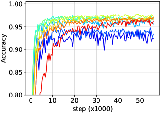
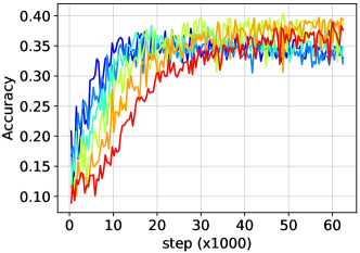
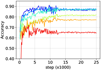
Test Acc. BA
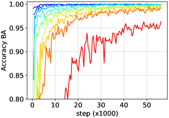
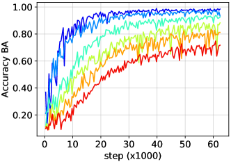
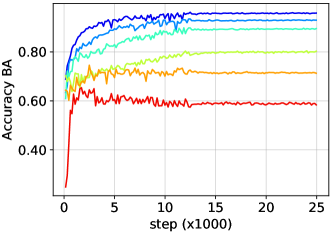
Test Acc. BC

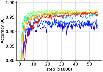
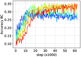
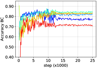
Figure 13: Test curves of Target Bias Adjustment (TBA) - our proposed extension of BiasBal [22] to deal with the unavailability of bias labels - w.r.t. different values of $\gamma$. Considered datasets are Colored MNIST, Corrupted CIFAR10, and Biased CelebA. All have BC ratios of 0.5%.

Appendix G Bias mitigation based on $p(b|u)$

G.1 Idea

In this section, we present an idea for mitigating bias by utilizing $p(b|u)$. We can estimate $p(b|u)$ via its proxy $p(b|y)$. When the bias attribute $b$ is discrete and the bias label is available, $p(b|y)$ can be estimated from the training data. However, in the case where $b$ is continuous or unknown, analytical computation of $p(b|y)$ become challenging. A possible workaround is computing $p(b_{n},u_{n}|y_{n})$ as an approximation of $p(b_{n}|y_{n})$ instead. This stems from the following equation:

$$p(b_{n},u_{n}|y_{n})=p(b_{n}|y_{n})p(u_{n}|b_{n},y_{n})\propto p(b_{n}|y_{n})$$ (23)

The last equation in Eq. 23 is based on the assumption $p(u_{n}|b_{n},y_{n})\approx p(u_{n}|y_{n})\propto 1$. Intuitively, this assumption implies that there is only one class-characteristic attribute associated with each class. As a result, once we know $y_{n}$, $u_{n}$ becomes deterministic and the randomness in $(b_{n},u_{n})$ is solely due to the randomness in $b_{n}$. While this assumption may be strict in general, it allows us to represent $(u_{n},b_{n})$ as a whole instead of extracting the bias attribute $b_{n}$ from $(u_{n},b_{n})$. If we consider $(u_{n},b_{n})$ as the latent representation $z_{n}$ of $x_{n}$ rather than $x_{n}$, then $p(u_{n},b_{n}|y_{n})$ becomes $p(z_{n}|y_{n})$. To compute $p(z|y)$, we design a conditional generative model that encompasses $p(z|y)$ as part of its generative process. This model is depicted in Fig. 14 (a) and has the joint distribution factorized as follows:

$$p_{\omega,\varphi}(x,z,y)=p_{\omega}(x|z)p_{\varphi}(z|y)p_{\mathcal{D}}(y)$$ (24)

where $p_{\varphi}(z|y)$ is modeled as an isotropic Gaussian distribution $\mathcal{N}(\mu_{y},\sigma_{y}^{2}\mathrm{I})$ with the learnable mean $\mu_{y}$ and standard deviation $\sigma_{y}$; $p_{\omega}(x|z)$ is modeled via a decoder network $D$ that maps $z$ to $x$. We learn this generative model by maximizing the sum of i) the variational lower bound (VLB) of $\log p_{\omega,\varphi}(x|y)$ w.r.t. the variational posterior distribution $q_{\phi}(z|x)$ and ii) the lower bound of $\log q_{\varphi,\phi}(y|x)$. $q_{\phi}(z|x)$ is modeled as an isotropic Gaussian $\mathcal{N}(\mu_{x},\sigma_{x}^{2}\mathrm{I})$ with the mean $\mu_{x}$ and standard deviation $\sigma_{x}$ being outputs of an encoder network $E$. $q_{\varphi,\phi}(y|x)$ computed as follows:

$$q_{\varphi,\phi}(y|x) =\int_{z}q_{\varphi,\phi}(y,z|x)\ dz$$ (25)

$$q_{\varphi,\phi}(y,z|x) =p_{\varphi}(y|z)q_{\phi}(z|x)$$ (26)

where $p_{\varphi}(y|z)$ is derived from $p_{\varphi}(z|y)$ as $p_{\varphi}(y|z)=\frac{p_{\varphi}(z|y)p_{\mathcal{D}}(y)}{\sum_{c=1}^{C}p_{\varphi}(z|c)p_{\mathcal{D}}(c)}$.

We name our proposed generative model “Variational Clustering Auto-Encoder” (VCAE). The loss function for training VCAE is given below:

$$\mathcal{L}_{\omega,\varphi,\phi}^{\text{VCAE}}(x,y):=\ \lambda_{0}\underbrace{\mathbb{E}_{q_{\phi}(z|x)}\left[-\log p_{\omega}(x|z)\right]}_{\text{reconstruction loss w.r.t. }x}+$$

$$\lambda_{1}\underbrace{D_{\text{KL}}\left(q_{\phi}(z|x)\|p_{\varphi}(z|y)\right)}_{\text{KL divergence w.r.t. }z}+$$

$$\lambda_{2}\underbrace{\mathbb{E}_{q_{\phi}(z|x)}\left[-\log p_{\varphi}(y|z)\right]}_{\text{cross-entropy loss w.r.t. }y}$$ (27)

where $\lambda_{0}$, $\lambda_{1}$, $\lambda_{2}$ $\geq 0$ are coefficients. When $\lambda_{0}$=$\lambda_{1}$=$\lambda_{2}$= 1, the first two terms in Eq. 27 form the negative of the VLB of $\log p_{\omega,\varphi}(x|y)$ while the last term is the negative of the lower bound of $\log q_{\varphi,\phi}(y|x)$. We provide the detailed mathematical derivations of these bounds in Appdx. G.3. The reconstruction loss encourages the encoder $E$ to capture both class and non-class attributes in $x$, the KL divergence forces latent representations of the same class to form a cluster that somewhat follows the Gaussian distribution, and the cross-entropy loss ensures that these clusters are well separate.

Once we have learned the parameters $\omega$, $\varphi$, $\phi$ by minimizing $\mathbb{E}_{p_{\mathcal{D}}(x,y)}\left[\mathcal{L}_{\omega,\varphi,\phi}^{\text{VCAE}}(x,y)\right]$, given an input-label pair $(x_{n},y_{n})$, we can sample $z_{n}$ from $q_{\phi}(z_{n}|x_{n})$ or simply set it to the mean $\mu_{x_{n}}$ of $q_{\phi}(z_{n}|x_{n})$. Then, we can compute $p_{\varphi}(z_{n}|y_{n})$ easily because it is the density of a Gaussian distribution. Intuitively, if we view $p_{\varphi}(z|y)$ as the distribution of points in the cluster centered at $\mu_{y}$, we would expect that the latent representations $z$ of bias-aligned (BA) samples should locate near $\mu_{y}$ and have large $p_{\varphi}(z|y)$ as these samples are abundant in the training data, while those of bias-conflicting (BC) samples should be far away from $\mu_{y}$ and have small $p_{\varphi}(z|y)$ due to the scarcity of BC samples. In the extreme case, the latent representations of BC samples can even be situated in the cluster of other classes if the BC samples contain non-class attributes $b$ that are highly correlated with those classes. This intuition is clearly depicted in Fig. 14 (b). From the figure, we can see that, the learned latent representations of BC samples of, for example, digit 0 (marked as red bordered squares) are not located within the cluster w.r.t. digit 0 (the red cluster) but within the clusters w.r.t. other digits (clusters with different colors) according to the background color of these BC samples.

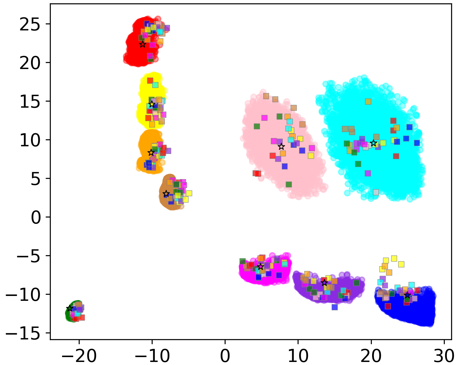
(a)	(b)	(c)

Figure 14: (a) Graphical representation of the Variational Clustering AutoEncoder. Observed variables are shaded. (b) Latent space of a VCAE with $\text{dim}(z)=2$ trained on the biased ColoredMNIST dataset (bias ratio $=$ 99.5%). Samples in the figure are colorized according to their class labels. Bias-aligned (BA) and bias-conflicting (BC) samples are distinguished by round and bordered square markers, respectively. (c) Histograms of the sample weights computed via VCAE for BA and BC samples. The formula for the weight $w_{n}$ of a sample $(x_{n},y_{n})$ is $w_{n}$=$\min\left(\frac{1}{p_{\varphi}(y_{n}|z_{n})},100\right)$.

However, although we can explicitly model and compute $p(z|y)$, it is still not straight-forward to use $p(z|y)$ for weighting. The main reason is that when $z$ is continuous, $p(z|y)$ is a probabilistic density function, and thus, is unnormalized (unlike the probability mass function). Another reason is that $p(z|y)$ becomes exponentially small when the dimension of $z$ increases, causing $\frac{1}{p(z|y)}$ to be exponentially large. These limitations of $p(z|y)$ are inherent, implying that we need to find alternative representations of $z$ that are well-normalized and stable. One possible solution to address this issue is using a collection of discrete latent codes (i.e., a codebook) to represent the latent space as in discrete VAE [51] or VQ-VAE [57]. In this case, $p(z|y)$ becomes a categorical distribution, and thus, is well-normalized and stable.

G.2 Using $p_{\varphi}(y|z)$ instead of $p_{\varphi}(z|y)$

We may consider using $p_{\varphi}(y|z)$ for weighting instead of $p_{\varphi}(z|y)$ since $p_{\varphi}(y|z)$ is well-normalized and stable. However, this technique is no longer associated with $p(b|u)$ but $p(u|b)$ (Section 3.1). It means that $z$, as a representation of $x$, should capture only the bias information $b$ in order to achieve good debiasing performance. In our experiments, we empirically observed that using $p(y|z)$ for bias mitigation, with $p(y|z)$ being modeled via a VCAE, only performs well on Colored MNIST when the VCAE has a small enough latent vector (e.g., dim($z$) < 10) and a large enough KL divergence coefficient (e.g., $\lambda_{1}\approx 1$) (Table 8 and Fig. G.2). This is because on Colored MNIST, the bias attribute (i.e., background color) accounts for most information in the input $x$, yet can be captured easily. Therefore, by using a small latent vector and a large KL divergence, VCAE is forced to learn a latent representation $z$ that focuses on capturing $b$ rather than $u$ in order to achieve a better reconstruction of $x$.

Dataset	BC (%)	Vanilla	LfF	PGD	LW
					$p(y|b)$	$p(y|z)$
Colored MNIST	0.5	80.18$\pm$1.38	93.38$\pm$0.52	96.15$\pm$0.28	95.57$\pm$0.41	96.85$\pm$0.16
	1.0	87.48$\pm$1.75	94.09$\pm$0.78	97.93$\pm$0.19	97.18$\pm$0.34	97.93$\pm$0.12
	5.0	97.04$\pm$0.21	97.40$\pm$0.25	98.74$\pm$0.12	98.61$\pm$0.09	98.18$\pm$0.11

Table 8: Results of LW with the sample weight computed based on $p(y|z)$ which is modeled by a VCAE in comparison with other baselines on Colored MNIST. Regarding the VCAE’s settings, $\text{dim}(z)=2$ and $(\lambda_{0},\lambda_{1},\lambda_{2})$ is set to (1, 1, 1).

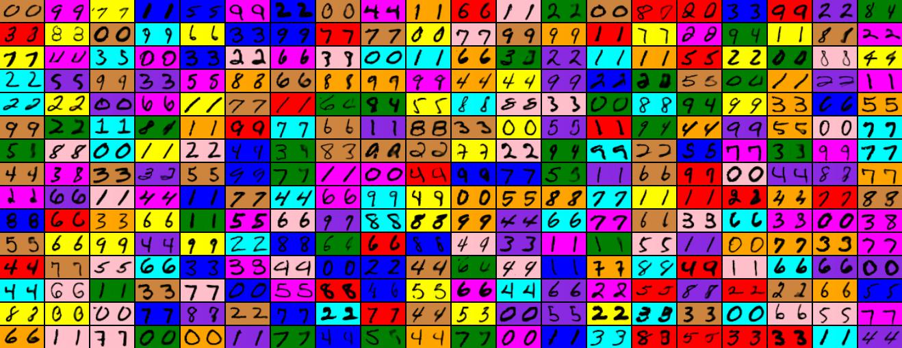
(a) dim($z$)=2	(b) dim($z$)=100

Figure 15: Pairs of original and reconstructed test BC images on Colored MNIST produced by VCAE. It is obvious that when dim($z$) = 2, the latent variable $z$ captures only the bias attribute (i.e., background color) since most of the reconstructed images contain incorrect class information.

G.3 Derivations of the lower bounds of $\log p_{\theta,\varphi}(x|y)$ and $\log q_{\varphi,\phi}(y|x)$

Given that $p_{\theta,\varphi}(x,z,y)=p_{\theta}(x|z)p_{\varphi}(z|y)p_{\mathcal{D}}(y)$ and $q_{\phi}(z|x)$ is the variational approximation of $p_{\theta,\varphi}(z|x,y)$, we can compute the variational lower bound of $p_{\theta,\varphi}(x|y)$ as follows:

$$\log p_{\theta,\varphi}(x|y)$$

$$=\ \mathbb{E}_{q_{\phi}(z|x)}\left[\log p_{\theta,\varphi}(x|y)\right]$$ (28)

$$=\ \mathbb{E}_{q_{\phi}(z|x)}\left[\log\frac{p_{\theta,\varphi}(x,z|y)}{p_{\theta,\varphi}(z|x,y)}\right]$$ (29)

$$=\ \mathbb{E}_{q_{\phi}(z|x)}\left[\log\frac{p_{\theta,\varphi}(x,z|y)}{q_{\phi}(z|x)}\right]+\mathbb{E}_{q_{\phi}(z|x)}\left[\log\frac{q_{\phi}(z|x)}{p_{\theta,\varphi}(z|x,y)}\right]$$ (30)

$$=\ \mathbb{E}_{q_{\phi}(z|x)}\left[\log\frac{p_{\theta,\varphi}(x,z|y)}{q_{\phi}(z|x)}\right]+D_{\text{KL}}\left(q_{\phi}(z|x)\|p_{\theta,\varphi}(z|x,y)\right)$$ (31)

$$\geq\ \mathbb{E}_{q_{\phi}(z|x)}\left[\log\frac{p_{\theta,\varphi}(x,z|y)}{q_{\phi}(z|x)}\right]$$ (32)

$$=\ \mathbb{E}_{q_{\phi}(z|x)}\left[\log\frac{p_{\theta}(x|z)p_{\varphi}(z|y)}{q_{\phi}(z|x)}\right]$$ (33)

$$=\ \mathbb{E}_{q_{\phi}(z|x)}\left[\log p_{\theta}(x|z)+\log p_{\varphi}(z|y)-\log q_{\phi}(z|x)\right]$$ (34)

$$=\ \mathbb{E}_{q_{\phi}(z|x)}\left[\log p_{\theta}(x|z)\right]-\mathbb{E}_{q_{\phi}(z|x)}\left[\log q_{\phi}(z|x)-\log p_{\varphi}(z|y)\right]$$ (35)

$$=\ \mathbb{E}_{q_{\phi}(z|x)}\left[\log p_{\theta}(x|z)\right]-D_{\text{KL}}\left(q_{\phi}(z|x)\|p_{\varphi}(z|y)\right)$$ (36)

where the inequality in Eq. 32 is due to the fact that $D_{\text{KL}}\left(q_{\phi}(z|x)\|p_{\theta,\varphi}(z|x,y)\right)\geq 0$.

We can also derive the lower bound of $\log q_{\varphi,\phi}(y|x)$ as follows:

$$\log q_{\varphi,\phi}(y|x) =\log\left(\int_{z}q_{\varphi,\phi}(y,z|x)\ dz\right)$$ (37)

$$=\log\left(\int_{z}p_{\varphi}(y|z)q_{\phi}(z|x)\ dz\right)$$ (38)

$$=\log\mathbb{E}_{q_{\phi}(z|x)}\left[p_{\varphi}(y|z)\right]$$ (39)

$$\geq\mathbb{E}_{q_{\phi}(z|x)}\left[\log p_{\varphi}(y|z)\right]$$ (40)

where the inequality in Eq. 40 is the Jensen’s inequality for the concave log function.

References

- [1] Aishwarya Agrawal, Dhruv Batra, and Devi Parikh. Analyzing the behavior of visual question answering models. In Proceedings of the 2016 Conference on Empirical Methods in Natural Language Processing, pages 1955–1960, 2016.
- [2] Aishwarya Agrawal, Dhruv Batra, Devi Parikh, and Aniruddha Kembhavi. Dont just assume; look and answer: Overcoming priors for visual question answering. In Proceedings of the IEEE conference on computer vision and pattern recognition, pages 4971–4980, 2018.
- [3] Sumyeong Ahn, Seongyoon Kim, and Se-young Yun. Mitigating dataset bias by using per-sample gradient. International Conference on Learning Representations, 2023.
- [4] Mohsan Alvi, Andrew Zisserman, and Christoffer Nellåker. Turning a blind eye: Explicit removal of biases and variation from deep neural network embeddings. In Proceedings of the European Conference on Computer Vision (ECCV) Workshops, pages 0–0, 2018.
- [5] Hyojin Bahng, Sanghyuk Chun, Sangdoo Yun, Jaegul Choo, and Seong Joon Oh. Learning de-biased representations with biased representations. In International Conference on Machine Learning, pages 528–539. PMLR, 2020.
- [6] Aharon Ben-Tal, Dick den Hertog, Anja De Waegenaere, Bertrand Melenberg, and Gijs Rennen. Robust solutions of optimization problems affected by uncertain probabilities. Management Science, 59(2):341–357, 2013.
- [7] Mateusz Buda, Atsuto Maki, and Maciej A Mazurowski. A systematic study of the class imbalance problem in convolutional neural networks. Neural networks, 106:249–259, 2018.
- [8] Remi Cadene, Corentin Dancette, Matthieu Cord, Devi Parikh, et al. Rubi: Reducing unimodal biases for visual question answering. Advances in neural information processing systems, 32, 2019.
- [9] Kaidi Cao, Colin Wei, Adrien Gaidon, Nikos Arechiga, and Tengyu Ma. Learning imbalanced datasets with label-distribution-aware margin loss. Advances in neural information processing systems, 32, 2019.
- [10] Nitesh V Chawla, Kevin W Bowyer, Lawrence O Hall, and W Philip Kegelmeyer. Smote: synthetic minority over-sampling technique. Journal of artificial intelligence research, 16:321–357, 2002.
- [11] Christopher Clark, Mark Yatskar, and Luke Zettlemoyer. Dont take the easy way out: Ensemble based methods for avoiding known dataset biases. In Proceedings of the 2019 Conference on Empirical Methods in Natural Language Processing and the 9th International Joint Conference on Natural Language Processing (EMNLP-IJCNLP), pages 4069–4082, 2019.
- [12] Yin Cui, Menglin Jia, Tsung-Yi Lin, Yang Song, and Serge Belongie. Class-balanced loss based on effective number of samples. In Proceedings of the IEEE/CVF conference on computer vision and pattern recognition, pages 9268–9277, 2019.
- [13] John Duchi, Peter Glynn, and Hongseok Namkoong. Statistics of robust optimization: A generalized empirical likelihood approach. arXiv preprint arXiv:1610.03425, 2016.
- [14] Charles Elkan. The foundations of cost-sensitive learning. In International joint conference on artificial intelligence, volume 17, pages 973–978. Lawrence Erlbaum Associates Ltd, 2001.
- [15] Andrew Estabrooks, Taeho Jo, and Nathalie Japkowicz. A multiple resampling method for learning from imbalanced data sets. Computational intelligence, 20(1):18–36, 2004.
- [16] Yaroslav Ganin, Evgeniya Ustinova, Hana Ajakan, Pascal Germain, Hugo Larochelle, François Laviolette, Mario Marchand, and Victor Lempitsky. Domain-adversarial training of neural networks. Journal of Machine Learning Research, 17:1–35, 2016.
- [17] Robert Geirhos, Patricia Rubisch, Claudio Michaelis, Matthias Bethge, Felix A Wichmann, and Wieland Brendel. Imagenet-trained cnns are biased towards texture; increasing shape bias improves accuracy and robustness. arXiv preprint arXiv:1811.12231, 2018.
- [18] Haibo He and Edwardo A Garcia. Learning from imbalanced data. IEEE Transactions on Knowledge and Data Engineering, 21(9):1263–1284, 2009.
- [19] Kaiming He, Xiangyu Zhang, Shaoqing Ren, and Jian Sun. Deep residual learning for image recognition. In Proceedings of the IEEE conference on computer vision and pattern recognition, pages 770–778, 2016.
- [20] Keisuke Hirano and Guido W Imbens. Estimation of causal effects using propensity score weighting: An application to data on right heart catheterization. Health Services and Outcomes research methodology, 2:259–278, 2001.
- [21] Keisuke Hirano, Guido W Imbens, and Geert Ridder. Efficient estimation of average treatment effects using the estimated propensity score. Econometrica, 71(4):1161–1189, 2003.
- [22] Youngkyu Hong and Eunho Yang. Unbiased classification through bias-contrastive and bias-balanced learning. Advances in Neural Information Processing Systems, 34:26449–26461, 2021.
- [23] Weihua Hu, Gang Niu, Issei Sato, and Masashi Sugiyama. Does distributionally robust supervised learning give robust classifiers? In International Conference on Machine Learning, pages 2029–2037. PMLR, 2018.
- [24] Inwoo Hwang, Sangjun Lee, Yunhyeok Kwak, Seong Joon Oh, Damien Teney, Jin-Hwa Kim, and Byoung-Tak Zhang. Selecmix: Debiased learning by contradicting-pair sampling. In Proceedings of the 36th Advances in Neural Information Processing Systems, 2022.
- [25] Sergey Ioffe and Christian Szegedy. Batch normalization: Accelerating deep network training by reducing internal covariate shift. In International conference on machine learning, pages 448–456. pmlr, 2015.
- [26] Salman Khan, Munawar Hayat, Syed Waqas Zamir, Jianbing Shen, and Ling Shao. Striking the right balance with uncertainty. In Proceedings of the IEEE/CVF Conference on Computer Vision and Pattern Recognition, pages 103–112, 2019.
- [27] Salman H Khan, Munawar Hayat, Mohammed Bennamoun, Ferdous A Sohel, and Roberto Togneri. Cost-sensitive learning of deep feature representations from imbalanced data. IEEE transactions on neural networks and learning systems, 29(8):3573–3587, 2017.
- [28] Aditya Khosla, Tinghui Zhou, Tomasz Malisiewicz, Alexei A Efros, and Antonio Torralba. Undoing the damage of dataset bias. In Computer Vision–ECCV 2012: 12th European Conference on Computer Vision, Florence, Italy, October 7-13, 2012, Proceedings, Part I 12, pages 158–171. Springer, 2012.
- [29] Byungju Kim, Hyunwoo Kim, Kyungsu Kim, Sungjin Kim, and Junmo Kim. Learning not to learn: Training deep neural networks with biased data. In Proceedings of the IEEE/CVF Conference on Computer Vision and Pattern Recognition, pages 9012–9020, 2019.
- [30] Eungyeup Kim, Jihyeon Lee, and Jaegul Choo. Biaswap: Removing dataset bias with bias-tailored swapping augmentation. In Proceedings of the IEEE/CVF International Conference on Computer Vision, pages 14992–15001, 2021.
- [31] Nayeong Kim, Sehyun Hwang, Sungsoo Ahn, Jaesik Park, and Suha Kwak. Learning debiased classifier with biased committee. In Proceedings of the 36th Advances in Neural Information Processing Systems, 2022.
- [32] Alex Krizhevsky, Geoffrey Hinton, et al. Learning multiple layers of features from tiny images. 2009.
- [33] Matjaz Kukar, Igor Kononenko, et al. Cost-sensitive learning with neural networks. In ECAI, volume 15, pages 88–94, 1998.
- [34] Steve Lawrence, Ian Burns, Andrew Back, Ah Chung Tsoi, and C Lee Giles. Neural network classification and prior class probabilities. Neural Networks: Tricks of the Trade: Second Edition, pages 295–309, 2012.
- [35] Ronan Le Bras, Swabha Swayamdipta, Chandra Bhagavatula, Rowan Zellers, Matthew Peters, Ashish Sabharwal, and Yejin Choi. Adversarial filters of dataset biases. In International conference on machine learning, pages 1078–1088. PMLR, 2020.
- [36] Yann LeCun, Corinna Cortes, Chris Burges, et al. Mnist handwritten digit database, 2010.
- [37] Jungsoo Lee, Eungyeup Kim, Juyoung Lee, Jihyeon Lee, and Jaegul Choo. Learning debiased representation via disentangled feature augmentation. Advances in Neural Information Processing Systems, 34:25123–25133, 2021.
- [38] Jungsoo Lee, Jeonghoon Park, Daeyoung Kim, Juyoung Lee, Edward Choi, and Jaegul Choo. Biasensemble: Revisiting the importance of amplifying bias for debiasing. Proceedings of the 37th AAAI Conference on Artificial Intelligence, 2023.
- [39] Yi Li and Nuno Vasconcelos. Repair: Removing representation bias by dataset resampling. In Proceedings of the IEEE/CVF conference on computer vision and pattern recognition, pages 9572–9581, 2019.
- [40] Yingwei Li, Yi Li, and Nuno Vasconcelos. Resound: Towards action recognition without representation bias. In Proceedings of the European Conference on Computer Vision (ECCV), pages 513–528, 2018.
- [41] Tsung-Yi Lin, Priya Goyal, Ross Girshick, Kaiming He, and Piotr Dollár. Focal loss for dense object detection. In Proceedings of the IEEE international conference on computer vision, pages 2980–2988, 2017.
- [42] Evan Z Liu, Behzad Haghgoo, Annie S Chen, Aditi Raghunathan, Pang Wei Koh, Shiori Sagawa, Percy Liang, and Chelsea Finn. Just train twice: Improving group robustness without training group information. In International Conference on Machine Learning, pages 6781–6792. PMLR, 2021.
- [43] Ziwei Liu, Ping Luo, Xiaogang Wang, and Xiaoou Tang. Deep learning face attributes in the wild. In Proceedings of International Conference on Computer Vision (ICCV), December 2015.
- [44] Chaochao Lu, Yuhuai Wu, José Miguel Hernández-Lobato, and Bernhard Schölkopf. Invariant causal representation learning for out-of-distribution generalization. In International Conference on Learning Representations, 2021.
- [45] Jovana Mitrovic, Brian McWilliams, Jacob Walker, Lars Buesing, and Charles Blundell. Representation learning via invariant causal mechanisms. arXiv preprint arXiv:2010.07922, 2020.
- [46] Junhyun Nam, Hyuntak Cha, Sungsoo Ahn, Jaeho Lee, and Jinwoo Shin. Learning from failure: De-biasing classifier from biased classifier. Advances in Neural Information Processing Systems, 33:20673–20684, 2020.
- [47] Toan Nguyen, Kien Do, Duc Thanh Nguyen, Bao Duong, and Thin Nguyen. Front-door adjustment via style transfer for out-of-distribution generalisation. arXiv preprint arXiv:2212.03063, 2022.
- [48] Taesung Park, Jun-Yan Zhu, Oliver Wang, Jingwan Lu, Eli Shechtman, Alexei Efros, and Richard Zhang. Swapping autoencoder for deep image manipulation. Advances in Neural Information Processing Systems, 33:7198–7211, 2020.
- [49] Judea Pearl et al. Models, reasoning and inference. Cambridge, UK: CambridgeUniversityPress, 19(2):3, 2000.
- [50] Sainandan Ramakrishnan, Aishwarya Agrawal, and Stefan Lee. Overcoming language priors in visual question answering with adversarial regularization. Advances in Neural Information Processing Systems, 31, 2018.
- [51] Jason Tyler Rolfe. Discrete variational autoencoders. arXiv preprint arXiv:1609.02200, 2016.
- [52] Donald B Rubin. Estimating causal effects of treatments in randomized and nonrandomized studies. Journal of educational Psychology, 66(5):688, 1974.
- [53] Shiori Sagawa, Pang Wei Koh, Tatsunori B Hashimoto, and Percy Liang. Distributionally robust neural networks for group shifts: On the importance of regularization for worst-case generalization. 2020.
- [54] Robik Shrestha, Kushal Kafle, and Christopher Kanan. An investigation of critical issues in bias mitigation techniques. In Proceedings of the IEEE/CVF Winter Conference on Applications of Computer Vision, pages 1943–1954, 2022.
- [55] Enzo Tartaglione, Carlo Alberto Barbano, and Marco Grangetto. End: Entangling and disentangling deep representations for bias correction. In Proceedings of the IEEE/CVF conference on computer vision and pattern recognition, pages 13508–13517, 2021.
- [56] A Torralba and AA Efros. Unbiased look at dataset bias. In Proceedings of the 2011 IEEE Conference on Computer Vision and Pattern Recognition, pages 1521–1528, 2011.
- [57] Aaron Van Den Oord, Oriol Vinyals, et al. Neural discrete representation learning. Advances in neural information processing systems, 30, 2017.
- [58] Vikas Verma, Alex Lamb, Christopher Beckham, Amir Najafi, Ioannis Mitliagkas, David Lopez-Paz, and Yoshua Bengio. Manifold mixup: Better representations by interpolating hidden states. In International conference on machine learning, pages 6438–6447. PMLR, 2019.
- [59] Haohan Wang, Eric P Xing, Zexue He, and Zachary C Lipton. Learning robust representations by projecting superficial statistics out. In International Conference on Learning Representations, ICLR 2019, 2019.
- [60] Ruoyu Wang, Mingyang Yi, Zhitang Chen, and Shengyu Zhu. Out-of-distribution generalization with causal invariant transformations. In Proceedings of the IEEE/CVF Conference on Computer Vision and Pattern Recognition, pages 375–385, 2022.
- [61] Liuyi Yao, Zhixuan Chu, Sheng Li, Yaliang Li, Jing Gao, and Aidong Zhang. A survey on causal inference. ACM Transactions on Knowledge Discovery from Data (TKDD), 15(5):1–46, 2021.
- [62] Zhongqi Yue, Qianru Sun, Xian-Sheng Hua, and Hanwang Zhang. Transporting causal mechanisms for unsupervised domain adaptation. In Proceedings of the IEEE/CVF International Conference on Computer Vision, pages 8599–8608, 2021.
- [63] Michael Zhang, Nimit S Sohoni, Hongyang R Zhang, Chelsea Finn, and Christopher Re. Correct-n-contrast: a contrastive approach for improving robustness to spurious correlations. In International Conference on Machine Learning, pages 26484–26516. PMLR, 2022.
- [64] Zhilu Zhang and Mert Sabuncu. Generalized cross entropy loss for training deep neural networks with noisy labels. Advances in neural information processing systems, 31, 2018.
- [65] Bolei Zhou, Aditya Khosla, Agata Lapedriza, Aude Oliva, and Antonio Torralba. Learning deep features for discriminative localization. In Proceedings of the IEEE conference on computer vision and pattern recognition, pages 2921–2929, 2016.
- [66] Wei Zhu, Haitian Zheng, Haofu Liao, Weijian Li, and Jiebo Luo. Learning bias-invariant representation by cross-sample mutual information minimization. In Proceedings of the IEEE/CVF International Conference on Computer Vision, pages 15002–15012, 2021.