How Does Unlabeled Data Provably Help
Out-of-Distribution Detection?

Abstract

Using unlabeled data to regularize the machine learning models has demonstrated promise for improving safety and reliability in detecting out-of-distribution (OOD) data. Harnessing the power of unlabeled in-the-wild data is non-trivial due to the heterogeneity of both in-distribution (ID) and OOD data. This lack of a clean set of OOD samples poses significant challenges in learning an optimal OOD classifier. Currently, there is a lack of research on formally understanding how unlabeled data helps OOD detection. This paper bridges the gap by introducing a new learning framework SAL (Separate And Learn) that offers both strong theoretical guarantees and empirical effectiveness. The framework separates candidate outliers from the unlabeled data and then trains an OOD classifier using the candidate outliers and the labeled ID data. Theoretically, we provide rigorous error bounds from the lens of separability and learnability, formally justifying the two components in our algorithm. Our theory shows that SAL can separate the candidate outliers with small error rates, which leads to a generalization guarantee for the learned OOD classifier. Empirically, SAL achieves state-of-the-art performance on common benchmarks, reinforcing our theoretical insights. Code is publicly available at https://github.com/deeplearning-wisc/sal.

1 Introduction

When deploying machine learning models in real-world environments, their safety and reliability are often challenged by the occurrence of out-of-distribution (OOD) data, which arise from unknown categories and should not be predicted by the model. Concerningly, neural networks are brittle and lack the necessary awareness of OOD data in the wild (Nguyen et al., 2015). Identifying OOD inputs is a vital but fundamentally challenging problem—the models are not explicitly exposed to the unknown distribution during training, and therefore cannot capture a reliable boundary between in-distribution (ID) vs. OOD data. To circumvent the challenge, researchers have started to explore training with additional data, which can facilitate a conservative and safe decision boundary against OOD data. In particular, a recent work by Katz-Samuels et al. (2022) proposed to leverage unlabeled data in the wild to regularize model training, while learning to classify labeled ID data. Such unlabeled wild data offer the benefits of being freely collectible upon deploying any machine learning model in its operating environment, and allow capturing the true test-time OOD distribution.

Despite the promise, harnessing the power of unlabeled wild data is non-trivial due to the heterogeneous mixture of ID and OOD data. This lack of a clean set of OOD training data poses significant challenges in designing effective OOD learning algorithms. Formally, the unlabeled data can be characterized by a Huber contamination model $\mathbb{P}_{\text{wild}}:=(1-\pi)\mathbb{P}_{\text{in}}+\pi\mathbb{P}_{\text{out}}$, where $\mathbb{P}_{\text{in}}$ and $\mathbb{P}_{\text{out}}$ are the marginal distributions of the ID and OOD data. It is important to note that the learner only observes samples drawn from such mixture distributions, without knowing the clear membership of whether being ID or OOD. Currently, a formalized understanding of the problem is lacking for the field. This prompts the question underlying the present work:

Algorithmic contribution. In this paper, we propose a new learning framework SAL (Separate And Learn), that effectively exploits the unlabeled wild data for OOD detection. At a high level, our framework SAL builds on two consecutive components: (1) filtering—separate candidate outliers from the unlabeled data, and (2) classification—learn an OOD classifier with the candidate outliers, in conjunction with the labeled ID data. To separate the candidate outliers, our key idea is to perform singular value decomposition on a gradient matrix, defined over all the unlabeled data whose gradients are computed based on a classification model trained on the clean labeled ID data. In the SAL framework, unlabeled wild data are considered candidate outliers when their projection onto the top singular vector exceeds a given threshold. The filtering strategy for identifying candidate outliers is theoretically supported by Theorem 1. We show in Section 3 (Remark 1) that under proper conditions, with a high probability, there exist some specific directions (e.g., the top singular vector direction) where the mean magnitude of the gradients for the wild outlier data is larger than that of ID data. After obtaining the outliers from the wild data, we train an OOD classifier that optimizes the classification between the ID vs. candidate outlier data for OOD detection.

Theoretical significance. Importantly, we provide new theories from the lens of separability and learnability, formally justifying the two components in our algorithm. Our main Theorem 1 analyzes the separability of outliers from unlabeled wild data using our filtering procedure, and gives a rigorous bound on the error rate. Our theory has practical implications. For example, when the size of the labeled ID data and unlabeled data is sufficiently large, Theorems 1 and 2 imply that the error rates of filtering outliers can be bounded by a small bias proportional to the optimal ID risk, which is a small value close to zero in reality (Frei et al., 2022). Based on the error rate estimation, we give a generalization error of the OOD classifier in Theorem 3, to quantify its learnability on the ID data and a noisy set of candidate outliers. Under proper conditions, the generalization error of the learned OOD classifier is upper bounded by the risk associated with the optimal OOD classifier.

Empirical validation. Empirically, we show that the generalization bound w.r.t. SAL (Theorem 3) indeed translates into strong empirical performance. SAL can be broadly applicable to non-convex models such as modern neural networks. We extensively evaluate SAL on common OOD detection tasks and establish state-of-the-art performance. For completeness, we compare SAL with two families of methods: (1) trained with only $\mathbb{P}_{\text{in}}$, and (2) trained with both $\mathbb{P}_{\text{in}}$ and an unlabeled dataset. On Cifar-100, compared to a strong baseline KNN+ (Sun et al., 2022) using only $\mathbb{P}_{\text{in}}$, SAL outperforms by 44.52% (FPR95) on average. While methods such as Outlier Exposure (Hendrycks et al., 2019) require a clean set of auxiliary unlabeled data, our results are achieved without imposing any such assumption on the unlabeled data and hence offer stronger flexibility. Compared to the most related baseline WOODS (Katz-Samuels et al., 2022), our framework can reduce the FPR95 from 7.80% to 1.88% on Cifar-100, establishing near-perfect results on this challenging benchmark.

2 Problem Setup

Formally, we describe the data setup, models and losses and learning goal.

Labeled ID data and ID distribution. Let $\mathcal{X}$ be the input space, and $\mathcal{Y}=\{1,...,K\}$ be the label space for ID data. Given an unknown ID joint distribution $\mathbb{P}_{\mathcal{X}\mathcal{Y}}$ defined over $\mathcal{X}\times\mathcal{Y}$, the labeled ID data $\mathcal{S}^{\text{in}}=\{(\mathbf{x}_{1},y_{1}),...,(\mathbf{x}_{n},y_{n})\}$ are drawn independently and identically from $\mathbb{P}_{\mathcal{X}\mathcal{Y}}$. We also denote $\mathbb{P}_{\text{in}}$ as the marginal distribution of $\mathbb{P}_{\mathcal{X}\mathcal{Y}}$ on $\mathcal{X}$, which is referred to as the ID distribution.

Out-of-distribution detection. Our framework concerns a common real-world scenario in which the algorithm is trained on the labeled ID data, but will then be deployed in environments containing OOD data from unknown class, i.e., $y\notin\mathcal{Y}$, and therefore should not be predicted by the model. At test time, the goal is to decide whether a test-time input is from ID or not (OOD).

Unlabeled wild data. A key challenge in OOD detection is the lack of labeled OOD data. In particular, the sample space for potential OOD data can be prohibitively large, making it expensive to collect labeled OOD data. In this paper, to model the realistic environment, we incorporate unlabeled wild data $\mathcal{S}_{\text{wild}}=\left\{\tilde{\mathbf{x}}_{1},...,\tilde{\mathbf{x}}_{m}\right\}$ into our learning framework. Wild data consists of both ID and OOD data, and can be collected freely upon deploying an existing model trained on $\mathcal{S}^{\text{in}}$. Following Katz-Samuels et al. (2022), we use the Huber contamination model to characterize the marginal distribution of the wild data

$$\mathbb{P}_{\text{wild}}:=(1-\pi)\mathbb{P}_{\text{in}}+\pi\mathbb{P}_{\text{out}},$$ (1)

where $\pi\in(0,1]$ and $\mathbb{P}_{\text{out}}$ is the OOD distribution defined over $\mathcal{X}$. Note that the case $\pi=0$ is straightforward since no novelties occur.

Models and losses. We denote by $\mathbf{h}_{\mathbf{w}}:\mathcal{X}\mapsto\mathbb{R}^{K}$ a predictor for ID classification with parameter $\mathbf{w}\in\mathcal{W}$, where $\mathcal{W}$ is the parameter space. $\mathbf{h}_{\mathbf{w}}$ returns the soft classification output. We consider the loss function $\ell:\mathbb{R}^{K}\times\mathcal{Y}\mapsto\mathbb{R}$ on the labeled ID data. In addition, we denote the OOD classifier $\mathbf{g}_{\bm{\theta}}:\mathcal{X}\mapsto\mathbb{R}$ with parameter ${\bm{\theta}}\in\Theta$, where $\Theta$ is the parameter space. We use $\ell_{\text{b}}(\mathbf{g}_{\bm{\theta}}(\mathbf{x}),y_{\text{b}})$ to denote the binary loss function w.r.t. $\mathbf{g}_{\bm{\theta}}$ and binary label $y_{\text{b}}\in\mathcal{Y}_{\text{b}}:=\{y_{+},y_{-}\}$, where $y_{+}\in\mathbb{R}_{>0}$ and $y_{-}\in\mathbb{R}_{<0}$ correspond to the ID class and the OOD class, respectively.

Learning goal. Our learning framework aims to build the OOD classifier $\mathbf{g}_{\bm{\theta}}$ by leveraging data from both $\mathcal{S}^{\text{in}}$ and $\mathcal{S}_{\text{wild}}$. In evaluating our model, we are interested in the following measurements:

$$(1)~{}\downarrow\text{FPR}(\mathbf{g}_{\bm{\theta}};\lambda):=\mathbb{E}_{\mathbf{x}\sim\mathbb{P}_{\text{out}}}(\mathds{1}{\{\mathbf{g}_{\bm{\theta}}(\mathbf{x})>\lambda\}}),$$ (2)

$$(2)~{}\uparrow\text{TPR}(\mathbf{g}_{\bm{\theta}};\lambda):=\mathbb{E}_{\mathbf{x}\sim\mathbb{P}_{\text{in}}}(\mathds{1}{\{\mathbf{g}_{\bm{\theta}}(\mathbf{x})>\lambda\}}),$$

where $\lambda$ is a threshold, typically chosen so that a high fraction of ID data is correctly classified.

3 Proposed Methodology

In this section, we introduce a new learning framework SAL that performs OOD detection by leveraging the unlabeled wild data. The framework offers substantial advantages over the counterpart approaches that rely only on the ID data, and naturally suits many applications where machine learning models are deployed in the open world. SAL has two integral components: (1) filtering—separate the candidate outlier data from the unlabeled wild data (Section 3.1), and (2) classification—train a binary OOD classifier with the ID data and candidate outliers (Section 3.2). In Section 4, we provide theoretical guarantees for SAL, provably justifying the two components in our method.

3.1 Separating Candidate Outliers from the Wild Data

To separate candidate outliers from the wild mixture $\mathcal{S}_{\text{wild}}$, our framework employs a level-set estimation based on the gradient information. The gradients are estimated from a classification predictor $\mathbf{h}_{\mathbf{w}}$ trained on the ID data $\mathcal{S}^{\text{in}}$. We describe the procedure formally below.

Estimating the reference gradient from ID data. To begin with, SAL estimates the reference gradients by training a classifier $\mathbf{h}_{\mathbf{w}}$ on the ID data $\mathcal{S}^{\text{in}}$ by empirical risk minimization (ERM):

$$\mathbf{w}_{\mathcal{S}^{\text{in}}}\in\operatorname*{arg\,min}_{\mathbf{w}\in\mathcal{W}}R_{\mathcal{S}^{\text{in}}}(\mathbf{h}_{\mathbf{w}}),~{}~{}\text{where}~{}~{}R_{\mathcal{S}^{\text{in}}}(\mathbf{h}_{\mathbf{w}})=\frac{1}{n}\sum_{(\mathbf{x}_{i},y_{i})\in\mathcal{S}^{\text{in}}}\ell(\mathbf{h}_{\mathbf{w}}(\mathbf{x}_{i}),y_{i}),$$ (3)

$\mathbf{w}_{\mathcal{S}^{\text{in}}}$ is the learned parameter and $n$ is the size of ID training set $\mathcal{S}^{\text{in}}$. The average gradient $\bar{\nabla}$ is

$$\bar{\nabla}=\frac{1}{n}\sum_{(\mathbf{x}_{i},y_{i})\in\mathcal{S}^{\text{in}}}\nabla\ell(\mathbf{h}_{\mathbf{w}_{\mathcal{S}^{\text{in}}}}(\mathbf{x}_{i}),y_{i}),$$ (4)

where $\bar{\nabla}$ acts as a reference gradient that allows measuring the deviation of any other points from it.

Separate candidate outliers from the unlabeled wild data. After training the classification predictor on the labeled ID data, we deploy the trained predictor $\mathbf{h}_{\mathbf{w}_{\mathcal{S}^{\text{in}}}}$ in the wild, and naturally receives data $\mathcal{S}_{\text{wild}}$—a mixture of unlabeled ID and OOD data. Key to our framework, we perform a filtering procedure on the wild data $\mathcal{S}_{\text{wild}}$, identifying candidate outliers based on a filtering score. To define the filtering score, we represent each point in $\mathcal{S}_{\text{wild}}$ as a gradient vector, relative to the reference gradient $\bar{\nabla}$. Specifically, we calculate the gradient matrix (after subtracting the reference gradient $\bar{\nabla}$) for the wild data as follows:

$$\mathbf{G}=\left[\begin{array}[]{c}\nabla\ell(\mathbf{h}_{\mathbf{w}_{\mathcal{S}^{\text{in}}}}(\tilde{\mathbf{x}}_{1}),\widehat{y}_{\tilde{\mathbf{x}}_{1}})-\bar{\nabla}\\ ...\\ \nabla\ell(\mathbf{h}_{\mathbf{w}_{\mathcal{S}^{\text{in}}}}(\tilde{\mathbf{x}}_{m}),\widehat{y}_{\tilde{\mathbf{x}}_{m}})-\bar{\nabla}\end{array}\right]^{\top},$$ (5)

where $m$ denotes the size of the wild data, and $\widehat{y}_{\tilde{\mathbf{x}}}$ is the predicted label for a wild sample $\tilde{\mathbf{x}}$. For each data point $\tilde{\mathbf{x}}_{i}$ in $\mathcal{S}_{\text{wild}}$, we then define our filtering score as follows:

$$\tau_{i}=\left<\nabla\ell(\mathbf{h}_{\mathbf{w}_{\mathcal{S}^{\text{in}}}}\big{(}\tilde{\mathbf{x}}_{i}),\widehat{y}_{\tilde{\mathbf{x}}_{i}})-\bar{\nabla},\mathbf{v}\right>^{2},$$ (6)

where $\left<\cdot,\cdot\right>$ is the dot product operator and $\mathbf{v}$ is the top singular vector of $\mathbf{G}$. The top singular vector $\mathbf{v}$ can be regarded as the principal component of the matrix $\mathbf{G}$ in Eq. 5, which maximizes the total distance from the projected gradients (onto the direction of $\mathbf{v}$) to the origin (sum over all points in $\mathcal{S}_{\text{wild}}$) (Hotelling, 1933). Specifically, $\mathbf{v}$ is a unit-norm vector and can be computed as follows:

$$\vspace{-0.1em}\mathbf{v}\in\operatorname*{arg\,max}_{\|\mathbf{u}\|_{2}=1}\sum_{\tilde{\mathbf{x}}_{i}\in\mathcal{S}_{\text{wild}}}\left<\mathbf{u},\nabla\ell(\mathbf{h}_{\mathbf{w}_{\mathcal{S}^{\text{in}}}}\big{(}\tilde{\mathbf{x}}_{i}),\widehat{y}_{\tilde{\mathbf{x}}_{i}})-\bar{\nabla}\right>^{2}.$$ (7)

Essentially, the filtering score $\tau_{i}$ in Eq. 6 measures the $\ell_{2}$ norm of the projected vector. To help readers better understand our design rationale, we provide an illustrative example of the gradient vectors and their projections in Figure 1 (see caption for details). Theoretically, Remark 1 below shows that the projection of the OOD gradient vector to the top singular vector of the gradient matrix $\mathbf{G}$ is on average provably larger than that of the ID gradient vector, which rigorously justifies our idea of using the score $\tau$ for separating the ID and OOD data.

Remark 1.

Theorem 4 in Appendix D.1 has shown that under proper assumptions, if we have sufficient data and large-size model, then with the high probability:

• the mean projected magnitude of OOD gradients in the direction of the top singular vector of $\mathbf{G}$ can be lower bounded by a positive constant $C/\pi$;

• the mean projected magnitude of ID gradients in the direction of the top singular vector is upper bounded by a small value close to zero.

Finally, we regard $\mathcal{S}_{T}=\{\tilde{\mathbf{x}}_{i}\in\mathcal{S}_{\text{wild}}:\mathbf{\tau}_{i}>T\}$ as the (potentially noisy) candidate outlier set, where $T$ is the filtering threshold. The threshold can be chosen on the ID data $\mathcal{S}^{\text{in}}$ so that a high fraction (e.g., 95%) of ID samples is below it. In Section 4, we will provide formal guarantees, rigorously justifying that the set $\mathcal{S}_{T}$ returns outliers with a large probability. We discuss and compare with alternative gradient-based scores (e.g., GradNorm (Huang et al., 2021)) for filtering in Section 5.2. In Appendix K, we discuss the variants of using multiple singular vectors, which yield similar results.

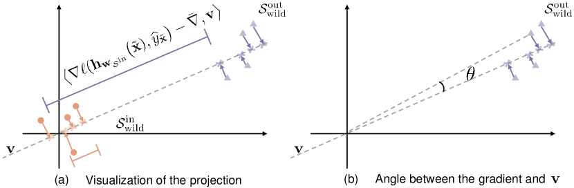
Figure 1: (a) Visualization of the gradient vectors, and their projection onto the top singular vector $\mathbf{v}$ (in gray dashed line). The gradients of inliers from $\mathcal{S}_{\text{wild}}^{\text{in}}$ (colored in orange) are close to the origin (reference gradient $\bar{\nabla}$). In contrast, the gradients of outliers from $\mathcal{S}_{\text{wild}}^{\text{out}}$ (colored in purple) are farther away. (b) The angle $\theta$ between the gradient of set $\mathcal{S}_{\text{wild}}^{\text{out}}$ and the singular vector $\mathbf{v}$. Since $\mathbf{v}$ is searched to maximize the distance from the projected points (cross marks) to the origin (sum over all the gradients in $\mathcal{S}_{\text{wild}}$), $\mathbf{v}$ points to the direction of OOD data in the wild with a small $\theta$. This further translates into a high filtering score $\tau$, which is essentially the norm after projecting a gradient vector onto $\mathbf{v}$. As a result, filtering outliers by $\mathcal{S}_{T}=\{\tilde{\mathbf{x}}_{i}\in\mathcal{S}_{\text{wild}}:\mathbf{\tau}_{i}>T\}$ will approximately return the purple OOD samples in the wild data.

An illustrative example of algorithm effect. To see the effectiveness of our filtering score, we test on two simulations in Figure 2 (a). These simulations are constructed with simplicity in mind, to facilitate understanding. Evaluations on complex high-dimensional data will be provided in Section 5. In particular, the wild data is a mixture of ID (multivariate Gaussian with three classes) and OOD. We consider two scenarios of OOD distribution, with ground truth colored in purple. Figure 2 (b) exemplifies the outliers (in green) identified using our proposed method, which largely aligns with the ground truth. The error rate of $\mathcal{S}_{T}$ containing ID data is only $8.4\%$ and $6.4\%$ for the two scenarios considered. Moreover, the filtering score distribution displays a clear separation between the ID vs. OOD parts, as evidenced in Figure 2 (c).

Remark 2. Our filtering process can be easily extended into $K$-class classification. In this case, one can maintain a class-conditional reference gradient $\bar{\nabla}_{k}$, one for each class $k\in[1,K]$, estimated on ID data belonging to class $k$, which captures the characteristics for each ID class. Similarly, the top singular vector computation can also be performed in a class-conditional manner, where we replace the gradient matrix with the class-conditional $\mathbf{G}_{k}$, containing gradient vectors of wild samples being predicted as class $k$.

3.2 Training the OOD Classifier with the Candidate Outliers

After obtaining the candidate outlier set $\mathcal{S}_{T}$ from the wild data, we train an OOD classifier $\mathbf{g}_{\bm{\theta}}$ that optimizes for the separability between the ID vs. candidate outlier data. In particular, our training objective can be viewed as explicitly optimizing the level-set based on the model output (threshold at 0), where the labeled ID data $\mathbf{x}$ from $\mathcal{S}^{\text{in}}$ has positive values and vice versa.

$$\begin{split}R_{\mathcal{S}^{\text{in}},\mathcal{S}_{T}}(\mathbf{g}_{\bm{\theta}})&=R_{\mathcal{S}^{\text{in}}}^{+}(\mathbf{g}_{\bm{\theta}})+R_{\mathcal{S}_{T}}^{-}(\mathbf{g}_{\bm{\theta}})\\ &=\mathbb{E}_{\mathbf{x}\in\mathcal{S}^{\text{in}}}~{}~{}\mathds{1}\{\mathbf{g}_{\bm{\theta}}(\mathbf{x})\leq 0\}+\mathbb{E}_{\tilde{\mathbf{x}}\in\mathcal{S}_{T}}~{}~{}\mathds{1}\{\mathbf{g}_{\bm{\theta}}(\tilde{\mathbf{x}})>0\}.\end{split}$$ (8)

To make the $0/1$ loss tractable, we replace it with the binary sigmoid loss, a smooth approximation of the $0/1$ loss. We train $\mathbf{g}_{\bm{\theta}}$ along with the ID risk in Eq. 3 to ensure ID accuracy. Notably, the training enables strong generalization performance for test OOD samples drawn from $\mathbb{P}_{\text{out}}$. We provide formal guarantees on the generalization bound in Theorem 3, as well as empirical support in Section 5. A pseudo algorithm of SAL is in Appendix (see Algorithm 1).

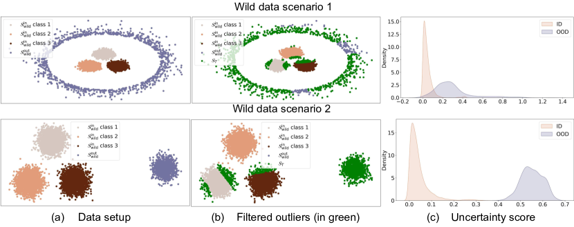
Figure 2: Example of SAL on two different scenarios of the unlabeled wild data. (a) Setup of the ID/inlier $\mathcal{S}_{\text{wild}}^{\text{in}}$ and OOD/outlier data $\mathcal{S}_{\text{wild}}^{\text{out}}$ in the wild. The inliers are sampled from three multivariate Gaussians. We construct two different distributions of outliers (see details in Appendix Q). (b) The filtered outliers (in green) by SAL, where the error rate of filtered outliers $\mathcal{S}_{T}$ containing inlier data is $8.4\%$ and $6.4\%$, respectively. (c) The density distribution of the filtering score $\tau$, which is separable for inlier and outlier data in the wild and thus benefits the training of the OOD classifier leveraging the filtered outlier data for binary classification.

4 Theoretical Analysis

We now provide theory to support our proposed algorithm. Our main theorems justify the two components in our algorithm. As an overview, Theorem 1 provides a provable bound on the error rates using our filtering procedure. Based on the estimations on error rates, Theorem 3 gives the generalization bound w.r.t. the empirical OOD classifier $\mathbf{g}_{\bm{\theta}}$, learned on ID data and noisy set of outliers. We specify several mild assumptions and necessary notations for our theorems in Appendix B. Due to space limitation, we omit unimportant constants and simplify the statements of our theorems. We defer the full formal statements in Appendix C. All proofs can be found in Appendices D and E.

4.1 Analysis on Separability

Our main theorem quantifies the separability of the outliers in the wild by using the filtering procedure (c.f. Section 3.1). Let $\text{ERR}_{\text{out}}$ and $\text{ERR}_{\text{in}}$ be the error rate of OOD data being regarded as ID and the error rate of ID data being regarded as OOD, i.e., $\text{ERR}_{\text{out}}=|\{\tilde{\mathbf{x}}_{i}\in\mathcal{S}^{\text{out}}_{\text{wild}}:\tau_{i}\leq T\}|/|\mathcal{S}^{\text{out}}_{\text{wild}}|$ and $\text{ERR}_{\text{in}}=|\{\tilde{\mathbf{x}}_{i}\in\mathcal{S}^{\text{in}}_{\text{wild}}:\tau_{i}>T\}|/|\mathcal{S}^{\text{in}}_{\text{wild}}|$, where $\mathcal{S}^{\text{in}}_{\text{wild}}$ and $\mathcal{S}^{\text{out}}_{\text{wild}}$ denote the sets of inliers and outliers from the wild data $\mathcal{S}_{\text{wild}}$. Then $\text{ERR}_{\text{out}}$ and $\text{ERR}_{\text{in}}$ have the following generalization bounds.

Practical implications of Theorem 1. The above theorem states that under mild assumptions, the errors $\text{ERR}_{\text{out}}$ and $\text{ERR}_{\text{in}}$ are upper bounded. For $\text{ERR}_{\text{in}}$, if the following two regulatory conditions hold: 1) the sizes of the labeled ID $n$ and wild data $m$ are sufficiently large; 2) the optimal ID risk $R_{\text{in}}^{*}$ is small, then the upper bound is tight. For $\text{ERR}_{\text{out}}$, $\delta(T)$ defined in Eq. 11 becomes the main error, if we have sufficient data. To further study the main error $\delta(T)$ in Eq. 10, Theorem 2 shows that the error $\delta(T)$ could be close to zero under practical conditions.

Practical implications of Theorem 2. Theorem 2 states that if the discrepancy $\zeta$ between two data distributions $\mathbb{P}_{\text{wild}}$ and $\mathbb{P}_{\text{in}}$ is larger than some small values, the main error $\delta(T)$ could be close to zero. Therefore, by combining with the two regulatory conditions mentioned in Theorem 1, the error $\text{ERR}_{\text{out}}$ could be close to zero. Empirically, we verify the conditions of Theorem 2 in Appendix F, which can hold true easily in practice. In addition, given fixed optimal ID risk $R_{\text{in}}^{*}$ and fixed sizes of the labeled ID $n$ and wild data $m$, we observe that the bound of ${\rm ERR}_{\text{in}}$ will increase when $\pi$ goes from 0 to 1. In contrast, the bound of ${\rm ERR}_{\text{out}}$ is non-monotonic when $\pi$ increases, which will firstly decrease and then increase. The observations align well with empirical results in Appendix F.

Impact of using predicted labels for the wild data. Recall in Section 3.1 that the filtering step uses the predicted labels to estimate the gradient for wild data, which is unlabeled. To analyze the impact theoretically, we show in Appendix Assumption 2 that the loss incurred by using the predicted label is smaller than the loss by using any label in the label space. This property is included in Appendix Lemmas 5 and 6 to constrain the filtering score in Appendix Theorem 5 and then filtering error in Theorem 1. In harder classification cases, the predicted label deviates more from the true label for the wild ID data, which leads to a looser bound for the filtering accuracy in Theorem 1.

Empirically, we calculate and compare the filtering accuracy and its OOD detection result on Cifar-10 and Cifar-100 ( Textures (Cimpoi et al., 2014) as the wild OOD). SAL achieves a result of $\rm ERR_{\text{in}}=0.018$ and $\rm ERR_{\text{out}}=0.17$ on Cifar-10 (easier classification case), which outperforms the result of $\rm ERR_{\text{in}}=0.037$ and $\rm ERR_{\text{out}}=0.30$ on Cifar-100 (harder classification case), aligning with our reasoning above. The experimental details are provided in Appendix P. Analysis of using random labels for the wild data is provided in Appendix O.

4.2 Analysis on Learnability

Leveraging the filtered outliers $\mathcal{S}_{T}$, SAL then trains an OOD classifier $\mathbf{g}_{\bm{\theta}}$ with the data from in-distribution $\mathcal{S}^{\text{in}}$ and data from $\mathcal{S}_{T}$ as OOD. In this section, we provide the generalization error bound for the learned OOD classifier to quantify its learnability. Specifically, we show that a small error guarantee in Theorem 1 implies that we can get a tight generalization error bound.

Insights. The above theorem presents the generalization error bound of the OOD classifier $\mathbf{g}_{\widehat{\bm{\theta}}_{T}}$ learned by using the filtered OOD data $\mathcal{S}_{T}$. When we have sufficient labeled ID data and wild data, then the risk of the OOD classifier $\mathbf{g}_{\widehat{\bm{\theta}}_{T}}$ is close to the optimal risk, i.e., $\min_{\bm{\theta}\in\Theta}R_{\mathbb{P}_{\text{in}},\mathbb{P}_{\text{out}}}(\mathbf{g}_{{\bm{\theta}}})$, if the optimal ID risk $R_{\text{in}}^{*}$ is small, and either one of the conditions in Theorem 2 is satisfied.

5 Experiments

In this section, we verify the effectiveness of our algorithm on modern neural networks. We aim to show that the generalization bound of the OOD classifier (Theorem 3) indeed translates into strong empirical performance, establishing state-of-the-art results (Section 5.2).

5.1 Experimental Setup

Datasets. We follow exactly the same experimental setup as WOODS (Katz-Samuels et al., 2022), which introduced the problem of learning OOD detectors with wild data. This allows us to draw fair comparisons. WOODS considered Cifar-10 and Cifar-100 (Krizhevsky et al., 2009) as ID datasets ($\mathbb{P}_{\text{in}}$). For OOD test datasets ($\mathbb{P}_{\text{out}}$), we use a suite of natural image datasets including Textures (Cimpoi et al., 2014), Svhn (Netzer et al., 2011), Places365 (Zhou et al., 2017), Lsun-Resize & Lsun-C (Yu et al., 2015). To simulate the wild data ($\mathbb{P}_{\text{wild}}$), we mix a subset of ID data (as $\mathbb{P}_{\text{in}}$) with the outlier dataset (as $\mathbb{P}_{\text{out}}$) under the default $\pi=0.1$, which reflects the practical scenario that most data would remain ID. Take Svhn as an example, we use Cifar+Svhn as the unlabeled wild data and test on Svhn as OOD. We simulate this for all OOD datasets and provide analysis of differing $\pi\in\{0.05,0.1,...,1.0\}$ in Appendix F. Note that we split Cifar datasets into two halves: $25,000$ images as ID training data, and the remainder $25,000$ for creating the wild mixture data. We use the weights from the penultimate layer for gradient calculation, which was shown to be the most informative for OOD detection (Huang et al., 2021). Experimental details are provided in Appendix G.

Evaluation metrics. We report the following metrics: (1) the false positive rate (FPR95$\downarrow$) of OOD samples when the true positive rate of ID samples is 95%, (2) the area under the receiver operating characteristic curve (AUROC$\uparrow$), and (3) ID classification Accuracy (ID ACC$\uparrow$).

Table 1: OOD detection performance on Cifar-100 as ID. All methods are trained on Wide ResNet-40-2 for 100 epochs. For each dataset, we create corresponding wild mixture distribution $\mathbb{P}_{\text{wild}}=(1-\pi)\mathbb{P}_{\text{in}}+\pi\mathbb{P}_{\text{out}}$ for training and test on the corresponding OOD dataset. Values are percentages averaged over 10 runs. Bold numbers highlight the best results. Table format credit to Katz-Samuels et al. (2022).

Methods	OOD Datasets												ID ACC
	Svhn		Places365		Lsun-C		Lsun-Resize		Textures		Average
	FPR95	AUROC	FPR95	AUROC	FPR95	AUROC	FPR95	AUROC	FPR95	AUROC	FPR95	AUROC
With $\mathbb{P}_{\text{in}}$ only
MSP	84.59	71.44	82.84	73.78	66.54	83.79	82.42	75.38	83.29	73.34	79.94	75.55	75.96
ODIN	84.66	67.26	87.88	71.63	55.55	87.73	71.96	81.82	79.27	73.45	75.86	76.38	75.96
Mahalanobis	57.52	86.01	88.83	67.87	91.18	69.69	21.23	96.00	39.39	90.57	59.63	82.03	75.96
Energy	85.82	73.99	80.56	75.44	35.32	93.53	79.47	79.23	79.41	76.28	72.12	79.69	75.96
KNN	66.38	83.76	79.17	71.91	70.96	83.71	77.83	78.85	88.00	67.19	76.47	77.08	75.96
ReAct	74.33	88.04	81.33	74.32	39.30	91.19	79.86	73.69	67.38	82.80	68.44	82.01	75.96
DICE	88.35	72.58	81.61	75.07	26.77	94.74	80.21	78.50	76.29	76.07	70.65	79.39	75.96
ASH	21.36	94.28	68.37	71.22	15.27	95.65	68.18	85.42	40.87	92.29	42.81	87.77	75.96
CSI	64.70	84.97	82.25	73.63	38.10	92.52	91.55	63.42	74.70	92.66	70.26	81.44	69.90
KNN+	32.21	93.74	68.30	75.31	40.37	86.13	44.86	88.88	46.26	87.40	46.40	86.29	73.78
With $\mathbb{P}_{\text{in}}$ and $\mathbb{P}_{\text{wild}}$
OE	1.57	99.63	60.24	83.43	3.83	99.26	0.93	99.79	27.89	93.35	18.89	95.09	71.65
Energy (w/ OE)	1.47	99.68	54.67	86.09	2.52	99.44	2.68	99.50	37.26	91.26	19.72	95.19	73.46
WOODS	0.12	99.96	29.58	90.60	0.11	99.96	0.07	99.96	9.12	96.65	7.80	97.43	75.22
SAL	0.07	99.95	3.53	99.06	0.06	99.94	0.02	99.95	5.73	98.65	1.88	99.51	73.71
(Ours)	±0.02	±0.00	±0.17	±0.06	±0.01	±0.21	±0.00	±0.03	±0.34	±0.02	±0.11	±0.02	±0.78

5.2 Empirical Results

SAL achieves superior empirical performance. We present results in Table 1 on Cifar-100, where SAL outperforms the state-of-the-art method. Our comparison covers an extensive collection of competitive OOD detection methods, which can be divided into two categories: trained with and without the wild data. For methods using ID data $\mathbb{P}_{\text{in}}$ only, we compare with methods such as MSP (Hendrycks & Gimpel, 2017), ODIN (Liang et al., 2018), Mahalanobis distance (Lee et al., 2018b), Energy score (Liu et al., 2020b), ReAct (Sun et al., 2021), DICE (Sun & Li, 2022), KNN distance (Sun et al., 2022), and ASH (Djurisic et al., 2023)—all of which use a model trained with cross-entropy loss. We also include the method based on contrastive loss, including CSI (Tack et al., 2020) and KNN+ (Sun et al., 2022). For methods using both ID and wild data, we compare with Outlier Exposure (OE) (Hendrycks et al., 2019) and energy-regularization learning (Liu et al., 2020b), which regularize the model by producing lower confidence or higher energy on the auxiliary outlier data. Closest to ours is WOODS (Katz-Samuels et al., 2022), which leverages wild data for OOD learning with a constrained optimization approach. For a fair comparison, all the methods in this group are trained using the same ID and in-the-wild data, under the same mixture ratio $\pi=0.1$.

The results demonstrate that: (1) Methods trained with both ID and wild data perform much better than those trained with only ID data. For example, on Places365, SAL reduces the FPR95 by 64.77% compared with KNN+, which highlights the advantage of using in-the-wild data for model regularization. (2) SAL performs even better compared to the competitive methods using $\mathbb{P}_{\text{wild}}$. On Cifar-100, SAL achieves an average FPR95 of 1.88%, which is a 5.92% improvement from WOODS. At the same time, SAL maintains a comparable ID accuracy. The slight discrepancy is due to that our method only observes 25,000 labeled ID samples, whereas baseline methods (without using wild data) utilize the entire Cifar training data with 50,000 samples. (3) The strong empirical performance achieved by SAL directly justifies and echoes our theoretical result in Section 4, where we showed the algorithm has a provably small generalization error. Overall, our algorithm enjoys both theoretical guarantees and empirical effectiveness.

Comparison with GradNorm as filtering score. Huang et al. (2021) proposed directly employing the vector norm of gradients, backpropagated from the KL divergence between the softmax output and a uniform probability distribution for OOD detection. Differently, our SAL derives the filtering score by performing singular value decomposition and using the norm of the projected gradient onto the top singular vector (c.f. Section 3.1). We compare SAL with a variant in Table 2, where we replace the filtering score in SAL with the GradNorm score and then train the OOD classifier. The result underperforms SAL, showcasing the effectiveness of our filtering score.

Table 2: Comparison with using GradNorm as the filtering score. We use Cifar-100 as ID. All methods are trained on Wide ResNet-40-2 for 100 epochs with $\pi=0.1$. Bold numbers are superior results.

Filter score	OOD Datasets												ID ACC
	Svhn		Places365		Lsun-C		Lsun-Resize		Textures		Average
	FPR95	AUROC	FPR95	AUROC	FPR95	AUROC	FPR95	AUROC	FPR95	AUROC	FPR95	AUROC
GradNorm	1.08	99.62	62.07	84.08	0.51	99.77	5.16	98.73	50.39	83.39	23.84	93.12	73.89
Ours	0.07	99.95	3.53	99.06	0.06	99.94	0.02	99.95	5.73	98.65	1.88	99.51	73.71

Additional ablations. Due to space limitations, we defer additional experiments in the Appendix, including (1) analyzing the effect of ratio $\pi$ (Appendix F), (2) results on Cifar-10 (Appendix H), (3) evaluation on unseen OOD datasets (Appendix I), (4) near OOD evaluations (Appendix J), and (5) the effect of using multiple singular vectors for calculating the filtering score (Appendix K) .

6 Related Work

OOD detection has attracted a surge of interest in recent years (Fort et al., 2021; Yang et al., 2021b; Fang et al., 2022; Zhu et al., 2022; Ming et al., 2022a; c; Yang et al., 2022; Wang et al., 2022b; Galil et al., 2023; Djurisic et al., 2023; Tao et al., 2023; Zheng et al., 2023; Wang et al., 2022a; 2023b; Narasimhan et al., 2023; Yang et al., 2023; Uppaal et al., 2023; Zhu et al., 2023b; a; Bai et al., 2023; Ming & Li, 2023; Zhang et al., 2023; Gu et al., 2023; Ghosal et al., 2024). One line of work performs OOD detection by devising scoring functions, including confidence-based methods (Bendale & Boult, 2016; Hendrycks & Gimpel, 2017; Liang et al., 2018), energy-based score (Liu et al., 2020b; Wang et al., 2021; Wu et al., 2023), distance-based approaches (Lee et al., 2018b; Tack et al., 2020; Ren et al., 2021; Sehwag et al., 2021; Sun et al., 2022; Du et al., 2022a; Ming et al., 2023; Ren et al., 2023), gradient-based score (Huang et al., 2021), and Bayesian approaches (Gal & Ghahramani, 2016; Lakshminarayanan et al., 2017; Maddox et al., 2019; Malinin & Gales, 2019; Wen et al., 2020; Kristiadi et al., 2020). Another line of work addressed OOD detection by training-time regularization (Bevandić et al., 2018; Malinin & Gales, 2018; Geifman & El-Yaniv, 2019; Hein et al., 2019; Meinke & Hein, 2020; Jeong & Kim, 2020; Liu et al., 2020a; van Amersfoort et al., 2020; Yang et al., 2021a; Wei et al., 2022; Du et al., 2022b; 2023; Wang et al., 2023a). For example, the model is regularized to produce lower confidence (Lee et al., 2018a; Hendrycks et al., 2019) or higher energy (Liu et al., 2020b; Du et al., 2022c; Ming et al., 2022b) on the outlier data. Most regularization methods assume the availability of a clean set of auxiliary OOD data. Several works (Zhou et al., 2021; Katz-Samuels et al., 2022; He et al., 2023) relaxed this assumption by leveraging the unlabeled wild data, but did not have an explicit mechanism for filtering the outliers. Compared to positive-unlabeled learning, which learns classifiers from positive and unlabeled data (Letouzey et al., 2000; Hsieh et al., 2015; Du Plessis et al., 2015; Niu et al., 2016; Gong et al., 2018; Chapel et al., 2020; Garg et al., 2021; Xu & Denil, 2021; Garg et al., 2022; Zhao et al., 2022; Acharya et al., 2022), the key difference is that it only considers the task of distinguishing $\mathbb{P}_{\text{out}}$ and $\mathbb{P}_{\text{in}}$, not the task of doing classification simultaneously. Moreover, we propose a new filtering score to separate outliers from the unlabeled data, which has a bounded error guarantee.

Robust statistics has systematically studied the estimation in the presence of outliers since the pioneering work of (Tukey, 1960). Popular methods include RANSAC (Fischler & Bolles, 1981), minimum covariance determinant (Rousseeuw & Driessen, 1999), Huberizing the loss (Owen, 2007), removal based on $k$-nearest neighbors (Breunig et al., 2000). More recently, there are several works that scale up the robust estimation into high-dimensions (Awasthi et al., 2014; Kothari & Steurer, 2017; Steinhardt, 2017; Diakonikolas & Kane, 2019; Diakonikolas et al., 2019a; 2022a; 2022b). Diakonikolas et al. (2019b) designed a gradient-based score for outlier removal but they focused on the error bound for the ID classifier. Instead, we provide new theoretical guarantees on outlier filtering (Theorem 1 and Theorem 2) and the generalization bound of OOD detection (Theorem 3).

7 Conclusion

In this paper, we propose a novel learning framework SAL that exploits the unlabeled in-the-wild data for OOD detection. SAL first explicitly filters the candidate outliers from the wild data using a new filtering score and then trains a binary OOD classifier leveraging the filtered outliers. Theoretically, SAL answers the question of how does unlabeled wild data help OOD detection by analyzing the separability of the outliers in the wild and the learnability of the OOD classifier, which provide provable error guarantees for the two integral components. Empirically, SAL achieves strong performance compared to competitive baselines, echoing our theoretical insights. A broad impact statement is included in Appendix V. We hope our work will inspire future research on OOD detection with unlabeled wild data.

How Does Unlabeled Data Provably
Help Out-of-Distribution Detection? (Appendix)

Appendix A Algorithm of SAL

We summarize our algorithm in implementation as follows.

Input: In-distribution data $\mathcal{S}^{\text{in}}=\left\{\left(\mathbf{x}_{i},y_{i}\right)\right\}_{i=1}^{n}$. Unlabeled wild data $\mathcal{S}_{\text{wild}}=\left\{\tilde{\mathbf{x}}_{i}\right\}_{i=1}^{m}$. $K$-way classification model $\mathbf{h}_{\mathbf{w}}$ and OOD classifier $\mathbf{g}_{\bm{\theta}}$. Parameter spaces $\mathcal{W}$ and $\Theta$. Learning rate lr for $\mathbf{g}_{\bm{\theta}}$.

Output: Learned OOD classifier $\mathbf{g}_{\widehat{\bm{\theta}}_{T}}$.

# Filtering stage

1) Perform ERM: $\mathbf{w}_{\mathcal{S}^{\text{in}}}\in\rm argmin_{\mathbf{w}\in\mathcal{W}}R_{\mathcal{S}^{\text{in}}}(\mathbf{h}_{\mathbf{w}})$.

2) Calculate the reference gradient as $\bar{\nabla}=\frac{1}{n}\sum_{(\mathbf{x}_{i},y_{i})\in\mathcal{S}^{\text{in}}}\nabla\ell(\mathbf{h}_{\mathbf{w}_{\mathcal{S}^{\text{in}}}}(\mathbf{x}_{i}),y_{i})$.

3) Calculate gradient on $\mathcal{S}_{\text{wild}}$ as $\nabla\ell(\mathbf{h}_{\mathbf{w}_{\mathcal{S}^{\text{in}}}}(\tilde{\mathbf{x}}_{i}),\widehat{y}_{\tilde{\mathbf{x}}_{i}})$ and calculate the gradient matrix $\mathbf{G}$.

4) Calculate the top singular vector $\mathbf{v}$ of $\mathbf{G}$ and the score $\tau_{i}=\left<\nabla\ell(\mathbf{h}_{\mathbf{w}_{\mathcal{S}^{\text{in}}}}\big{(}\tilde{\mathbf{x}}_{i}),\widehat{y}_{\tilde{\mathbf{x}}_{i}})-\bar{\nabla},\mathbf{v}\right>^{2}$.

5) Get the candidate outliers $\mathcal{S}_{T}=\{\tilde{\mathbf{x}}_{i}\in\mathcal{S}_{\text{wild}},\tau_{i}\geq T\}$.

# Training Stage

for epoch in epochs do

       6) Sample batches of data ${\mathcal{B}^{\text{in}},\mathcal{B}_{T}}$ from ID and candidate outliers ${\mathcal{S}^{\text{in}},\mathcal{S}_{T}}$.

       7) Calculate the binary classification loss $R_{\mathcal{B}^{\text{in}},\mathcal{B}_{T}}(\mathbf{g}_{\bm{\theta}})$.

       8) Update the parameter by $\widehat{\bm{\theta}}_{T}=\bm{\theta}-{\rm lr}\cdot\nabla R_{\mathcal{B}^{\text{in}},\mathcal{B}_{T}}(\mathbf{g}_{\bm{\theta}})$.

end for

Algorithm 1 SAL: Separate And Learn

Appendix B Notations, Definitions, Assumptions and Important Constants

Here we summarize the important notations and constants in Tables 3 and 4, restate necessary definitions and assumptions in Sections B.2 and B.3.

B.1 Notations

Please see Table 3 for detailed notations.

Table 3: Main notations and their descriptions.

Notation	Description
Spaces
$\mathcal{X}$, $\mathcal{Y}$	the input space and the label space.
$\mathcal{W}$, $\Theta$	the hypothesis spaces
Distributions
$\mathbb{P}_{\text{wild}}$, $\mathbb{P}_{{\text{in}}}$, $\mathbb{P}_{{\text{out}}}$	data distribution for wild data, labeled ID data and OOD data
$\mathbb{P}_{\mathcal{X}\mathcal{Y}}$	the joint data distribution for ID data.
Data and Models
$\mathbf{w}$, $\mathbf{x}$, $\mathbf{v}$	weight/input/the top-1 right singular vector of $G$
$\widehat{\nabla}$, $\tau$	the average gradients on labeled ID data, uncertainty score
$y$ and $y_{\text{b}}$	label for ID classification and binary label for OOD detection
$\widehat{y}_{\mathbf{x}}$	Predicted one-hot label for input $\mathbf{x}$
$\mathbf{h}_{\mathbf{w}}$ and $\mathbf{g}_{\bm{\theta}}$	predictor on labeled in-distribution and binary predictor for OOD detection
$\mathcal{S}_{{\text{wild}}}^{\text{in}}$, $\mathcal{S}_{{\text{wild}}}^{\text{out}}$	inliers and outliers in the wild dataset.
$\mathcal{S}^{\text{in}}$, $\mathcal{S}_{\text{wild}}$	labeled ID data and unlabeled wild data
$n$, $m$	size of $\mathcal{S}^{\text{in}}$, size of $\mathcal{S}_{\text{wild}}$
$T$	the filtering threshold
$\mathcal{S}_{T}$	wild data whose uncertainty score higher than threshold $T$
Distances
$r_{1}$ and $r_{2}$	the radius of the hypothesis spaces $\mathcal{W}$ and $\Theta$, respectively
$\|\cdot\|_{2}$	$\ell_{2}$ norm
Loss, Risk and Predictor
$\ell(\cdot,\cdot)$, $\ell_{\text{b}}(\cdot,\cdot)$	ID loss function, binary loss function
$R_{\mathcal{S}}(\mathbf{h}_{\mathbf{w}})$	the empirical risk w.r.t. predictor $\mathbf{h}_{\mathbf{w}}$ over data $\mathcal{S}$
$R_{\mathbb{P}_{\mathcal{X}\mathcal{Y}}}(\mathbf{h}_{\mathbf{w}})$	the risk w.r.t. predictor $\mathbf{h}_{\mathbf{w}}$ over joint distribution $\mathbb{P}_{\mathcal{X}\mathcal{Y}}$
$R_{\mathbb{P}_{\text{in}},\mathbb{P}_{\text{out}}}(\mathbf{g}_{{\bm{\theta}}})$	the risk defined in Eq. 14
${\rm ERR}_{\text{in}},{\rm ERR}_{\text{out}}$	the error rates of regarding ID as OOD and OOD as ID

B.2 Definitions

Definition 1 ($\beta$-smooth).

We say a loss function $\ell(\mathbf{h}_{\mathbf{w}}(\mathbf{x}),y)$ (defined over $\mathcal{X}\times\mathcal{Y}$) is $\beta$-smooth, if for any $\mathbf{x}\in\mathcal{X}$ and $y\in\mathcal{Y}$,

$$\big{\|}\nabla\ell(\mathbf{h}_{\mathbf{w}}(\mathbf{x}),y)-\nabla\ell(\mathbf{h}_{\mathbf{w}^{\prime}}(\mathbf{x}),y)\big{\|}_{2}\leq\beta\|\mathbf{w}-\mathbf{w}^{\prime}\|_{2}$$

    

Definition 2 (Gradient-based Distribution Discrepancy).

Given distributions $\mathbb{P}$ and $\mathbb{Q}$ defined over $\mathcal{X}$, the Gradient-based Distribution Discrepancy w.r.t. predictor $\mathbf{h}_{\mathbf{w}}$ and loss $\ell$ is

$$d_{\mathbf{w}}^{\ell}(\mathbb{P},\mathbb{Q})=\big{\|}\nabla R_{\mathbb{P}}(\mathbf{h}_{\mathbf{w}},\widehat{\mathbf{h}})-\nabla R_{\mathbb{Q}}(\mathbf{h}_{\mathbf{w}},\widehat{\mathbf{h}})\big{\|}_{2},$$ (15)

where $\widehat{\mathbf{h}}$ is a classifier which returns the closest one-hot vector of $\mathbf{h}_{\mathbf{w}}$, $R_{\mathbb{P}}(\mathbf{h}_{\mathbf{w}},\widehat{\mathbf{h}})=\mathbb{E}_{\mathbf{x}\sim\mathbb{P}}\ell(\mathbf{h}_{\mathbf{w}},\widehat{\mathbf{h}})$ and $R_{\mathbb{Q}}(\mathbf{h}_{\mathbf{w}},\widehat{\mathbf{h}})=\mathbb{E}_{\mathbf{x}\sim\mathbb{Q}}\ell(\mathbf{h}_{\mathbf{w}},\widehat{\mathbf{h}})$.

Definition 3 ($(\gamma,\zeta)$-discrepancy).

We say a wild distribution $\mathbb{P}_{\text{wild}}$ has $(\gamma,\zeta)$-discrepancy w.r.t. an ID joint distribution $\mathbb{P}_{\text{in}}$, if $\gamma>\min_{\mathbf{w}\in\mathcal{W}}R_{\mathbb{P}_{\mathcal{X}\mathcal{Y}}}(\mathbf{h}_{\mathbf{w}})$, and for any parameter $\mathbf{w}\in\mathcal{W}$ satisfying that $R_{\mathbb{P}_{\mathcal{X}\mathcal{Y}}}(\mathbf{h}_{\mathbf{w}})\leq\gamma$ should meet the following condition

$$d_{\mathbf{w}}^{\ell}(\mathbb{P}_{\text{in}},\mathbb{P}_{\text{wild}})>\zeta,$$

where $R_{\mathbb{P}_{\mathcal{X}\mathcal{Y}}}(\mathbf{h}_{\mathbf{w}})=\mathbb{E}_{(\mathbf{x},y)\sim\mathbb{P}_{\mathcal{X}\mathcal{Y}}}\ell(\mathbf{h}_{\mathbf{w}}(\mathbf{x}),y)$.

In Section F, we empirically calculate the values of the distribution discrepancy between the ID joint distribution $\mathbb{P}_{\mathcal{X}\mathcal{Y}}$ and the wild distribution $\mathbb{P}_{\text{wild}}$.    

B.3 Assumptions

Assumption 1.

    

• The parameter space $\mathcal{W}\subset B(\mathbf{w}_{0},r_{1})\subset\mathbb{R}^{d}$ ($\ell_{2}$ ball of radius $r_{1}$ around $\mathbf{w}_{0}$);

• The parameter space $\Theta\subset B(\bm{\theta}_{0},r_{2})\subset\mathbb{R}^{d^{\prime}}$ ($\ell_{2}$ ball of radius $r_{2}$ around $\bm{\theta}_{0}$);

• $\ell(\mathbf{h}_{\mathbf{w}}(\mathbf{x}),y)\geq 0$ and $\ell(\mathbf{h}_{\mathbf{w}}(\mathbf{x}),y)$ is $\beta_{1}$-smooth;

• $\ell_{\text{b}}(\mathbf{g}_{\bm{\theta}}(\mathbf{x}),y_{\text{b}})\geq 0$ and $\ell_{\text{b}}(\mathbf{g}_{\bm{\theta}}(\mathbf{x}),y_{\text{b}})$ is $\beta_{2}$-smooth;

• $\sup_{(\mathbf{x},y)\in\mathcal{X}\times\mathcal{Y}}\|\nabla\ell(\mathbf{h}_{\mathbf{w}_{0}}(\mathbf{x}),y)\|_{2}=b_{1}$, $\sup_{(\mathbf{x},y_{\text{b}})\in\mathcal{X}\times\mathcal{Y}_{\text{b}}}\|\nabla\ell(\mathbf{g}_{\bm{\theta}_{0}}(\mathbf{x}),y_{\text{b}})\|_{2}=b_{2}$;

• $\sup_{(\mathbf{x},y)\in\mathcal{X}\times\mathcal{Y}}\ell(\mathbf{h}_{\mathbf{w}_{0}}(\mathbf{x}),y)=B_{1}$, $\sup_{(\mathbf{x},y_{\text{b}})\in\mathcal{X}\times\mathcal{Y}_{\text{b}}}\ell(\mathbf{g}_{\bm{\theta}_{0}}(\mathbf{x}),y_{\text{b}})=B_{2}$.

Remark 2.

For neural networks with smooth activation functions and softmax output function, we can check that the norm of the second derivative of the loss functions (cross-entropy loss and sigmoid loss) is bounded given the bounded parameter space, which implies that the $\beta$-smoothness of the loss functions can hold true. Therefore, our assumptions are reasonable in practice.

Assumption 2.

$\ell(\mathbf{h}(\mathbf{x}),\widehat{y}_{\mathbf{x}})\leq\min_{y\in\mathcal{Y}}\ell(\mathbf{h}(\mathbf{x}),{y}),$ where $\widehat{y}_{\mathbf{x}}$ returns the closest one-hot label of the predictor $\mathbf{h}$’s output on $\mathbf{x}$.

Remark 3.

The assumption means the loss incurred by using the predicted labels given by the classifier itself is smaller or equal to the loss incurred by using any label in the label space. If $y=\widehat{y}_{\mathbf{x}}$, the assumption is satisfied obviously. If $y\neq\widehat{y}_{\mathbf{x}}$, then we provide two examples to illustrate the validity of the assumption. For example, (1) if the loss $\ell$ is the cross entropy loss, let $K=2,\mathbf{h}(\mathbf{x})=[h_{1},h_{2}]$ (classification output after softmax) and $h_{1}>h_{2}$. Therefore, we have $\widehat{y}_{\mathbf{x}}=0$. Suppose $y=1$, we can get $\ell(\mathbf{h}(\mathbf{x}),\widehat{y}_{\mathbf{x}})=-\operatorname{log}(h_{1})<\ell(\mathbf{h}(\mathbf{x}),y)=-\operatorname{log}(h_{2})$. (2) If $\ell$ is the hinge loss for binary classification, thus we have $K=1$, let $\mathbf{h}(\mathbf{x})=h_{1}<0$ and thus $\widehat{y}_{\mathbf{x}}=-1$. Suppose $y=1$, we can get $\ell(\mathbf{h}(\mathbf{x}),\widehat{y}_{\mathbf{x}})=\operatorname{max}(0,1+h_{1})<\operatorname{max}(0,1-h_{1})=\ell(\mathbf{h}(\mathbf{x}),y).$

B.4 Constants in Theory

Table 4: Constants in theory.

Constants	Description
$M=\beta_{1}r_{1}^{2}+b_{1}r_{1}+B_{1}$	the upper bound of loss $\ell(\mathbf{h}_{\mathbf{w}}(\mathbf{x}),y)$, see Proposition 1
$M^{\prime}=2(\beta_{1}r_{1}+b_{1})^{2}$	the upper bound of filtering score $\tau$
$\tilde{M}=\beta_{1}M$	a constant for simplified representation
$L=\beta_{2}r_{2}^{2}+b_{2}r_{2}+B_{2}$	the upper bound of loss $\ell_{\text{b}}(\mathbf{g}_{\bm{\theta}}(\mathbf{x}),y_{\text{b}})$, see Proposition 1
$d$, $d^{\prime}$	the dimensions of parameter spaces $\mathcal{W}$ and $\Theta$, respectively
$R^{*}_{{\text{in}}}$	the optimal ID risk, i.e., $R^{*}_{{\text{in}}}=\min_{\mathbf{w}\in\mathcal{W}}\mathbb{E}_{(\mathbf{x},y)\sim\mathbb{P}_{\mathcal{X}\mathcal{Y}}}\ell(\mathbf{h}_{\mathbf{w}}(\mathbf{x}),y)$
$\delta(T)$	the main error in Eq. 10
$\zeta$	the discrepancy between $\mathbb{P}_{\text{in}}$ and $\mathbb{P}_{\text{wild}}$
$\pi$	the ratio of OOD distribution in $\mathbb{P}_{\text{wild}}$

Appendix C Main Theorems

In this section, we provide a detailed and formal version of our main theorems with a complete description of the constant terms and other additional details that are omitted in the main paper.

Theorem 1.

If Assumptions 1 and 2 hold, $\mathbb{P}_{\text{wild}}$ has $(\gamma,\zeta)$-discrepancy w.r.t. $\mathbb{P}_{\mathcal{X}\mathcal{Y}}$, and there exists $\eta\in(0,1)$ s.t. $\Delta=(1-\eta)^{2}\zeta^{2}-8\beta_{1}R_{{\text{in}}}^{*}>0$, then for

$$n=\Omega\big{(}\frac{\tilde{M}+M(r_{1}+1)d}{\eta^{2}\Delta}+\frac{M^{2}{d}}{(\gamma-R_{\text{in}}^{*})^{2}}\big{)},~{}~{}~{}~{}~{}m=\Omega\big{(}\frac{\tilde{M}+M(r_{1}+1)d}{\eta^{2}\zeta^{2}}\big{)},$$

with the probability at least $9/10$, for any $0<T<M^{\prime}$ $($here $M^{\prime}=2(\beta_{1}r_{1}+b_{1})^{2}$ is the upper bound of filtering score $\tau_{i}$, i.e., $\tau_{i}\leq M^{\prime}$$)$,

$${\rm ERR}_{\text{in}}\leq\frac{8\beta_{1}}{T}R_{\text{in}}^{*}+O\Big{(}\frac{\tilde{M}}{T}\sqrt{\frac{d}{n}}\Big{)}+O\Big{(}\frac{\tilde{M}}{T}\sqrt{\frac{d}{(1-\pi)m}}\Big{)},$$ (16)

$$\begin{split}{\rm ERR}_{\text{out}}&\leq\delta(T)+O\Big{(}\frac{\tilde{M}}{1-T/M^{\prime}}\sqrt{\frac{d}{{\pi}^{2}n}}\Big{)}\\ &+O\Big{(}\frac{\max\{{\tilde{M}\sqrt{d}},\Delta_{\zeta}^{\eta}/\pi\}}{1-T/M^{\prime}}\sqrt{\frac{1}{{\pi}^{2}(1-\pi)m}}\Big{)},\end{split}$$ (17)

where $R^{*}_{{\text{in}}}$ is the optimal ID risk, i.e., $R^{*}_{{\text{in}}}=\min_{\mathbf{w}\in\mathcal{W}}\mathbb{E}_{(\mathbf{x},y)\sim\mathbb{P}_{\mathcal{X}\mathcal{Y}}}\ell(\mathbf{h}_{\mathbf{w}}(\mathbf{x}),y)$,

$$\begin{split}\delta(T)&=\frac{\max\{0,1-\Delta_{\zeta}^{\eta}/\pi\}}{(1-T/M^{\prime})},~{}~{}~{}\Delta_{\zeta}^{\eta}={0.98\eta^{2}\zeta^{2}}-8\beta_{1}R_{\text{in}}^{*},\\ &M=\beta_{1}r_{1}^{2}+b_{1}r_{1}+B_{1},~{}~{}~{}\tilde{M}=M\beta_{1},\end{split}$$ (18)

and $d$ is the dimension of the parameter space $\mathcal{W}$, here $\beta_{1},r_{1},B_{1}$ are given in Assumption 1.

           

Theorem 2.

1) If $\Delta_{\zeta}^{\eta}\geq(1-\epsilon)\pi$ for a small error $\epsilon\geq 0$, then the main error $\delta(T)$ defined in Eq. 11 satisfies that

$$\delta(T)\leq\frac{\epsilon}{1-T/{M^{\prime}}}.$$

2) If $\zeta\geq 2.011\sqrt{8\beta_{1}R_{\text{in}}^{*}}+1.011\sqrt{\pi}$, then there exists $\eta\in(0,1)$ ensuring that $\Delta>0$ and $\Delta_{\zeta}^{\eta}>\pi$ hold, which implies that the main error $\delta(T)=0$.

           

Theorem 3.

Given the same conditions in Theorem 1, if we further require that

$$n=\Omega\Big{(}\frac{\tilde{M}^{2}d}{\min\{\pi,\Delta_{\zeta}^{\eta}\}^{2}}\Big{)},~{}~{}~{}m=\Omega\Big{(}\frac{\tilde{M}^{2}d+\Delta_{\zeta}^{\eta}}{\pi^{2}(1-\pi)\min\{\pi,\Delta_{\zeta}^{\eta}\}^{2}}\Big{)},$$

then with the probability at least $89/100$, for any $0<T<0.9M^{\prime}\min\{1,\Delta_{\zeta}^{\eta}/\pi\}$, the OOD classifier $\mathbf{g}_{\widehat{\bm{\theta}}_{T}}$ learned by the proposed algorithm satisfies the following risk estimation

$$R_{\mathbb{P}_{\text{in}},\mathbb{P}_{\text{out}}}(\mathbf{g}_{\widehat{\bm{\theta}}_{T}})\leq\inf_{\bm{\theta}\in\Theta}R_{\mathbb{P}_{\text{in}},\mathbb{P}_{\text{out}}}(\mathbf{g}_{{\bm{\theta}}})+\frac{3.5L}{1-\delta(T)}\delta({T})+\frac{9(1-\pi)L\beta_{1}}{\pi(1-\delta(T))T}R_{\text{in}}^{*}$$ (19)

$$+ O\Big{(}\frac{L\max\{\tilde{M}\sqrt{d},\sqrt{d^{\prime}}\}}{\min\{\pi,\Delta_{\zeta}^{\eta}\}T^{\prime}}\sqrt{\frac{1}{n}}\Big{)}+O\Big{(}\frac{L\max\{\tilde{M}\sqrt{d},\sqrt{d^{\prime}},\Delta_{\zeta}^{\eta}\}}{\min\{\pi,\Delta_{\zeta}^{\eta}\}T^{\prime}}\sqrt{\frac{1}{\pi^{2}(1-\pi)m}}\Big{)},$$

where $R_{\text{in}}^{*}$, $\Delta_{\zeta}^{\eta}$, $M$, $M^{\prime}$, $\tilde{M}$ and $d$ are shown in Theorem 1, $d^{\prime}$ is the dimension of space $\Theta$,

$$L=\beta_{2}r_{2}^{2}+b_{2}r_{2}+B_{2},~{}~{}~{}T^{\prime}=T/(1+T),$$

and the risk $R_{\mathbb{P}_{\text{in}},\mathbb{P}_{\text{out}}}(\mathbf{g}_{{\bm{\theta}}})$ is defined as follows:

$$R_{\mathbb{P}_{\text{in}},\mathbb{P}_{\text{out}}}(\mathbf{g}_{\widehat{\bm{\theta}}_{T}})=\mathbb{E}_{\mathbf{x}\sim\mathbb{P}_{\text{in}}}\ell_{\text{b}}(\mathbf{g}_{\bm{\theta}}(\mathbf{x}),y_{+})+\mathbb{E}_{\mathbf{x}\sim\mathbb{P}_{\text{out}}}\ell_{\text{b}}(\mathbf{g}_{\bm{\theta}}(\mathbf{x}),y_{-}).$$

           

Theorem 4.

Given the same conditions in Theorem 1, with the probability at least $9/10$,

$$\begin{split}\mathbb{E}_{\tilde{\mathbf{x}}_{i}\sim\mathcal{S}_{\text{wild}}^{\text{in}}}\tau_{i}\leq&8\beta_{1}R_{\text{in}}^{*}+O(\beta_{1}M\sqrt{\frac{d}{n}})+O(\beta_{1}M\sqrt{\frac{d}{(1-\pi)m}}),\end{split}$$

$$\begin{split}\mathbb{E}_{\tilde{\mathbf{x}}_{i}\sim\mathcal{S}_{\text{wild}}^{\text{out}}}\tau_{i}\geq&\frac{0.98\eta^{2}\zeta^{2}}{\pi}-\frac{8\beta_{1}R_{\text{in}}^{*}}{\pi}-\epsilon^{\prime}(n,m),\end{split}$$

furthermore, if the realizability assumption for ID distribution holds (Shalev-Shwartz & Ben-David, 2014; Fang et al., 2022), then

$$\mathbb{E}_{\tilde{\mathbf{x}}_{i}\sim\mathcal{S}_{\text{wild}}^{\text{in}}}\tau_{i}\leq O(\beta_{1}M\sqrt{\frac{d}{n}})+O(\beta_{1}M\sqrt{\frac{d}{(1-\pi)m}})$$

$$\begin{split}\mathbb{E}_{\tilde{\mathbf{x}}_{i}\sim\mathcal{S}_{\text{wild}}^{\text{out}}}\tau_{i}\geq&\frac{0.98\eta^{2}\zeta^{2}}{\pi}-\epsilon^{\prime}(n,m),\end{split}$$

where

$$\epsilon^{\prime}(n,m)\leq O(\frac{\beta_{1}M}{\pi}\sqrt{\frac{d}{n}})+O\Big{(}({{\beta_{1}M\sqrt{d}}+\sqrt{1-\pi}\Delta_{\zeta}^{\eta}/\pi})\sqrt{\frac{1}{{\pi}^{2}(1-\pi)m}}\Big{)},$$

and $R_{\text{in}}^{*}$, $\Delta_{\zeta}^{\eta}$, $M$ and $d$ are shown in Theorem 1.

Appendix D Proofs of Main Theorems

D.1 Proof of Theorem 1

Step 1. With the probability at least $1-\frac{7}{3}\delta>0$,

$$\begin{split}\mathbb{E}_{\tilde{\mathbf{x}}_{i}\sim\mathcal{S}_{\text{wild}}^{\text{in}}}\tau_{i}\leq&8\beta_{1}R_{\text{in}}^{*}\\ +&4\beta_{1}\Big{[}C\sqrt{\frac{Mr_{1}(\beta_{1}r_{1}+b_{1})d}{n}}+C\sqrt{\frac{Mr_{1}(\beta_{1}r_{1}+b_{1})d}{(1-\pi)m-\sqrt{m\log(6/\delta)/2}}}\\ &+3M\sqrt{\frac{2\log(6/\delta)}{n}}+M\sqrt{\frac{2\log(6/\delta)}{(1-\pi)m-\sqrt{m\log(6/\delta)/2}}}\Big{]},\end{split}$$

This can be proven by Lemma 7 and following inequality

$$\begin{split}&\mathbb{E}_{\tilde{\mathbf{x}}_{i}\sim\mathcal{S}_{\text{wild}}^{\text{in}}}\tau_{i}\leq\mathbb{E}_{\tilde{\mathbf{x}}_{i}\sim\mathcal{S}_{\text{wild}}^{\text{in}}}\big{\|}\nabla\ell(\mathbf{h}_{\mathbf{w}_{\mathcal{S}^{\text{in}}}}(\tilde{\mathbf{x}}_{i}),\widehat{\mathbf{h}}_{\mathbf{w}_{\mathcal{S}^{\text{in}}}}(\tilde{\mathbf{x}}_{i}))-\mathbb{E}_{(\mathbf{x}_{j},y_{j})\sim\mathcal{S}^{\operatorname{in}}}\nabla\ell(\mathbf{h}_{\mathbf{w}_{\mathcal{S}^{\text{in}}}}(\mathbf{x}_{j}),y_{j})\big{\|}_{2}^{2},\end{split}$$

Step 2. It is easy to check that

$$\mathbb{E}_{\tilde{\mathbf{x}}_{i}\sim\mathcal{S}_{\text{wild}}}\tau_{i}=\frac{|\mathcal{S}_{\text{wild}}^{\text{in}}|}{|\mathcal{S}_{\text{wild}}|}\mathbb{E}_{\tilde{\mathbf{x}}_{i}\sim\mathcal{S}_{\text{wild}}^{\text{in}}}\tau_{i}+\frac{|\mathcal{S}_{\text{wild}}^{\text{out}}|}{|\mathcal{S}_{\text{wild}}|}\mathbb{E}_{\tilde{\mathbf{x}}_{i}\sim\mathcal{S}_{\text{wild}}^{\text{out}}}\tau_{i}.$$

Step 3. Let

$$\begin{split}\epsilon(n,m)=&4\beta_{1}[C\sqrt{\frac{Mr_{1}(\beta_{1}r_{1}+b_{1})d}{n}}+C\sqrt{\frac{Mr_{1}(\beta_{1}r_{1}+b_{1})d}{(1-\pi)m-\sqrt{m\log(6/\delta)/2}}}\\ +&3M\sqrt{\frac{2\log(6/\delta)}{n}}+M\sqrt{\frac{2\log(6/\delta)}{(1-\pi)m-\sqrt{m\log(6/\delta)/2}}}].\end{split}$$

Under the condition in Theorem 5, with the probability at least $\frac{97}{100}-\frac{7}{3}\delta>0$,

$$\begin{split}\mathbb{E}_{\tilde{\mathbf{x}}_{i}\sim\mathcal{S}_{\text{wild}}^{\text{out}}}\tau_{i}\geq&\frac{m}{|\mathcal{S}_{\text{wild}}^{\text{out}}|}\big{[}\frac{98\eta^{2}\zeta^{2}}{100}-\frac{|\mathcal{S}_{\text{wild}}^{\text{in}}|}{m}8\beta_{1}R_{\text{in}}^{*}-\frac{|\mathcal{S}_{\text{wild}}^{\text{in}}|}{m}\epsilon(n,m)\big{]}\\ \geq&\frac{m}{|\mathcal{S}_{\text{wild}}^{\text{out}}|}\big{[}\frac{98\eta^{2}\zeta^{2}}{100}-8\beta_{1}R_{\text{in}}^{*}-\epsilon(n,m)\big{]}\\ \geq&\big{[}\frac{1}{\pi}-\frac{\sqrt{\log{6/\delta}}}{\pi^{2}\sqrt{2m}+\pi\sqrt{\log(6/\delta)}}\big{]}\big{[}\frac{98\eta^{2}\zeta^{2}}{100}-8\beta_{1}R_{\text{in}}^{*}-\epsilon(n,m)\big{]}.\end{split}$$

In this proof, we set

$$\Delta(n,m)=\big{[}\frac{1}{\pi}-\frac{\sqrt{\log{6/\delta}}}{\pi^{2}\sqrt{2m}+\pi\sqrt{\log(6/\delta)}}\big{]}\big{[}\frac{98\eta^{2}\zeta^{2}}{100}-8\beta_{1}R_{\text{in}}^{*}-\epsilon(n,m)\big{]}.$$

Note that $\Delta_{\zeta}^{\eta}={0.98\eta^{2}\zeta^{2}}-8\beta_{1}R_{\text{in}}^{*}$, then

$$\Delta(n,m)=\frac{1}{\pi}\Delta_{\zeta}^{\eta}-\frac{1}{\pi}\epsilon(n,m)-\Delta_{\zeta}^{\eta}\epsilon(m)+\epsilon(n)\epsilon(n,m),$$

where $\epsilon(m)={\sqrt{\log{6/\delta}}}/({\pi^{2}\sqrt{2m}+\pi\sqrt{\log(6/\delta)}})$.

Step 4. Under the condition in Theorem 5, with the probability at least $\frac{97}{100}-\frac{7}{3}\delta>0$,

$$\frac{|\{\tilde{\mathbf{x}}_{i}\in\mathcal{S}_{\operatorname{wild}}^{\operatorname{out}}:\tau_{i}\leq T\}|}{|\mathcal{S}_{\operatorname{wild}}^{\operatorname{out}}|}\leq\frac{1-\min\{1,\Delta(n,m)\}}{1-T/{M^{\prime}}},$$ (20)

and

$$\frac{|\{\tilde{\mathbf{x}}_{i}\in\mathcal{S}_{\operatorname{wild}}^{\operatorname{in}}:\tau_{i}>T\}|}{|\mathcal{S}_{\operatorname{wild}}^{\operatorname{in}}|}\leq\frac{8\beta_{1}R_{\text{in}}^{*}+\epsilon(n,m)}{T}.$$ (21)

We prove this step: let $Z$ be the uniform random variable with $\mathcal{S}_{\operatorname{wild}}^{\operatorname{out}}$ as its support and $Z(i)=\tau_{i}/(2(\beta_{1}r_{1}+b_{1})^{2})$, then by the Markov inequality, we have

$$\frac{|\{\tilde{\mathbf{x}}_{i}\in\mathcal{S}_{\operatorname{wild}}^{\operatorname{out}}:\tau_{i}>T\}|}{|\mathcal{S}_{\operatorname{wild}}^{\operatorname{out}}|}=P(Z(i)>T/(2(\beta_{1}r_{1}+b_{1})^{2}))\geq\frac{\Delta(n,m)-T/(2(\beta_{1}r_{1}+b_{1})^{2})}{1-T/(2(\beta_{1}r_{1}+b_{1})^{2})}.$$ (22)

Let $Z$ be the uniform random variable with $\mathcal{S}_{\operatorname{wild}}^{\operatorname{in}}$ as its support and $Z(i)=\tau_{i}$, then by the Markov inequality, we have

$$\frac{|\{\tilde{\mathbf{x}}_{i}\in\mathcal{S}_{\operatorname{wild}}^{\operatorname{in}}:\tau_{i}>T\}|}{|\mathcal{S}_{\operatorname{wild}}^{\operatorname{in}}|}=P(Z(i)>T)\leq\frac{\mathbb{E}[Z]}{T}=\frac{8\beta_{1}R_{\text{in}}^{*}+\epsilon(n,m)}{T}.$$ (23)

Step 5. If $\pi\leq\Delta_{\zeta}^{\eta}/(1-\epsilon/{M^{\prime}})$, then with the probability at least $\frac{97}{100}-\frac{7}{3}\delta>0$,

$$\frac{|\{\tilde{\mathbf{x}}_{i}\in\mathcal{S}_{\operatorname{wild}}^{\operatorname{out}}:\tau_{i}\leq T\}|}{|\mathcal{S}_{\operatorname{wild}}^{\operatorname{out}}|}\leq\frac{\epsilon+M^{\prime}\epsilon^{\prime}(n,m)}{M^{\prime}-T},$$ (24)

and

$$\frac{|\{\tilde{\mathbf{x}}_{i}\in\mathcal{S}_{\operatorname{wild}}^{\operatorname{in}}:\tau_{i}>T\}|}{|\mathcal{S}_{\operatorname{wild}}^{\operatorname{in}}|}\leq\frac{8\beta_{1}R_{\text{in}}^{*}+\epsilon(n,m)}{T},$$ (25)

where $\epsilon^{\prime}(n,m)={\epsilon(n,m)}/{\pi}+\Delta_{\zeta}^{\eta}\epsilon(m)-\epsilon(n)\epsilon(n,m)$.

Step 6. If we set $\delta=3/100$, then it is easy to see that

$$\begin{split}&\epsilon(m)\leq O(\frac{1}{\pi^{2}\sqrt{m}}),\\ &\epsilon(n,m)\leq O(\beta_{1}M\sqrt{\frac{d}{n}})+O(\beta_{1}M\sqrt{\frac{d}{(1-\pi)m}}),\\ &\epsilon^{\prime}(n,m)\leq O(\frac{\beta_{1}M}{\pi}\sqrt{\frac{d}{n}})+O\Big{(}({{\beta_{1}M\sqrt{d}}+\sqrt{1-\pi}\Delta_{\zeta}^{\eta}/\pi})\sqrt{\frac{1}{{\pi}^{2}(1-\pi)m}}\Big{)}.\end{split}$$

Step 7. By results in Steps 4, 5 and 6, We complete this proof.

D.2 Proof of Theorem 2

The first result is trivial. Hence, we omit it. We mainly focus on the second result in this theorem. In this proof, then we set

$$\eta={\sqrt{8\beta_{1}R_{\text{in}}^{*}+0.99\pi}}/({\sqrt{0.98}\sqrt{8\beta_{1}R_{\text{in}}^{*}}+\sqrt{8\beta_{1}R_{\text{in}}^{*}+\pi}})$$

Note that it is easy to check that

$$\zeta\geq 2.011\sqrt{8\beta_{1}R_{\text{in}}^{*}}+1.011\sqrt{\pi}\geq\sqrt{8\beta_{1}R_{\text{in}}^{*}}+1.011\sqrt{8\beta_{1}R_{\text{in}}^{*}+\pi}.$$

Therefore,

$$\eta\zeta\geq\frac{1}{\sqrt{0.98}}\sqrt{8\beta_{1}R_{\text{in}}^{*}+0.99\pi}>\sqrt{8\beta_{1}R_{\text{in}}^{*}+\pi},$$

which implies that $\Delta_{\zeta}^{\eta}>\pi$. Note that

$$\begin{split}(1-\eta)\zeta&\geq\frac{1}{\sqrt{0.98}}\big{(}{{\sqrt{0.98}\sqrt{8\beta_{1}R_{\text{in}}^{*}}+\sqrt{8\beta_{1}R_{\text{in}}^{*}+\pi}}-{\sqrt{8\beta_{1}R_{\text{in}}^{*}+0.99\pi}}}\big{)}>\sqrt{8\beta_{1}R_{\text{in}}^{*}},\end{split}$$

which implies that $\Delta>0$. We have completed this proof.  

D.3 Proof of Theorem 3

Let

$$\bm{\theta}^{*}\in\operatorname*{arg\,min}_{\bm{\theta}\in\Theta}R_{\mathbb{P}_{\text{in}},\mathbb{P}_{\text{out}}}(\bm{\theta}).$$

Then by Lemma 1 and Lemma 14, we obtain that with the high probability

$$\begin{split}&R_{\mathbb{P}_{\text{in}},\mathbb{P}_{\text{out}}}(\mathbf{g}_{\widehat{\bm{\theta}}_{T}})-R_{\mathbb{P}_{\text{in}},\mathbb{P}_{\text{out}}}(\mathbf{g}_{{\bm{\theta}}^{*}})\\ =&R_{\mathbb{P}_{\text{in}},\mathbb{P}_{\text{out}}}(\mathbf{g}_{\widehat{\bm{\theta}}_{T}})-R_{\mathcal{S}^{\text{in}},\mathcal{S}_{T}}(\mathbf{g}_{\widehat{\bm{\theta}}_{T}})+R_{\mathcal{S}^{\text{in}},\mathcal{S}_{T}}(\mathbf{g}_{\widehat{\bm{\theta}}_{T}})-R_{\mathcal{S}^{\text{in}},\mathcal{S}_{T}}(\mathbf{g}_{{\bm{\theta}}^{*}})\\ +&R_{\mathcal{S}^{\text{in}},\mathcal{S}_{T}}(\mathbf{g}_{{\bm{\theta}}^{*}})-R_{\mathbb{P}_{\text{in}},\mathbb{P}_{\text{out}}}(\mathbf{g}_{{\bm{\theta}}^{*}})\\ \leq&R_{\mathbb{P}_{\text{in}},\mathbb{P}_{\text{out}}}(\mathbf{g}_{\widehat{\bm{\theta}}_{T}})-R_{\mathcal{S}^{\text{in}},\mathcal{S}_{T}}(\mathbf{g}_{\widehat{\bm{\theta}}_{T}})\\ +&R_{\mathcal{S}^{\text{in}},\mathcal{S}_{T}}(\mathbf{g}_{{\bm{\theta}}^{*}})-R_{\mathbb{P}_{\text{in}},\mathbb{P}_{\text{out}}}(\mathbf{g}_{{\bm{\theta}}^{*}})\\ \leq&2\sup_{\bm{\theta}\in\Theta}\big{|}R_{\mathcal{S}^{\text{in}}}^{+}(\mathbf{g}_{{\bm{\theta}}})-R_{\mathbb{P}_{\text{in}}}^{+}(\mathbf{g}_{{\bm{\theta}}})\big{|}\\ +&\sup_{\bm{\theta}\in\Theta}\big{(}R_{\mathcal{S}^{\text{out}}}^{-}(\mathbf{g}_{{\bm{\theta}}})-R_{\mathbb{P}_{\text{out}}}^{-}(\mathbf{g}_{{\bm{\theta}}})\big{)}+\sup_{\bm{\theta}\in\Theta}\big{(}R_{\mathbb{P}_{\text{out}}}^{-}(\mathbf{g}_{{\bm{\theta}}})-R_{\mathcal{S}^{\text{out}}}^{-}(\mathbf{g}_{{\bm{\theta}}})\big{)}\\ \leq&\frac{3.5L}{1-\delta(T)}\delta({T})+\frac{9(1-\pi)L\beta_{1}}{\pi(1-\delta(T))T}R_{\text{in}}^{*}\\ +&O\Big{(}\frac{L\max\{\beta_{1}M\sqrt{d},\sqrt{d^{\prime}}\}(1+T)}{\min\{\pi,\Delta_{\zeta}^{\eta}\}T}\sqrt{\frac{1}{n}}\Big{)}\\ +&O\Big{(}\frac{L\max\{\beta_{1}M\sqrt{d},\sqrt{d^{\prime}},\Delta_{\zeta}^{\eta}\}(1+T)}{\min\{\pi,\Delta_{\zeta}^{\eta}\}T}\sqrt{\frac{1}{\pi^{2}(1-\pi)m}}\Big{)},\end{split}$$

 

D.4 Proof of Theorem 4

The result is induced by the Steps 1, 3 and 6 in Proof of Theorem 1 (see section D.1).

Appendix E Necessary Lemmas, Propositions and Theorems

E.1 Boundedness

Proposition 1.

If Assumption 1 holds,

$$\sup_{\mathbf{w}\in\mathcal{W}}\sup_{(\mathbf{x},y)\in\mathcal{X}\times\mathcal{Y}}\|\nabla\ell(\mathbf{h}_{\mathbf{w}}(\mathbf{x}),y)\|_{2}\leq\beta_{1}r_{1}+b_{1}=\sqrt{{M^{\prime}}/{2}},$$

$$\sup_{\bm{\theta}\in\Theta}\sup_{(\mathbf{x},y_{\text{b}})\in\mathcal{X}\times\mathcal{Y}_{\text{b}}}\|\nabla\ell(\mathbf{g}_{\bm{\theta}}(\mathbf{x}),y_{\text{b}})\|_{2}\leq\beta_{2}r_{2}+b_{2}.$$

$$\begin{split}&\sup_{\mathbf{w}\in\mathcal{W}}\sup_{(\mathbf{x},y)\in\mathcal{X}\times\mathcal{Y}}\ell(\mathbf{h}_{\mathbf{w}}(\mathbf{x}),y)\leq\beta_{1}r_{1}^{2}+b_{1}r_{1}+B_{1}=M,\end{split}$$

$$\begin{split}&\sup_{\bm{\theta}\in\Theta}\sup_{(\mathbf{x},y_{\text{b}})\in\mathcal{X}\times\mathcal{Y}_{\text{b}}}\ell_{\text{b}}(\mathbf{g}_{\bm{\theta}}(\mathbf{x}),y_{\text{b}})\leq\beta_{2}r_{2}^{2}+b_{2}r_{2}+B_{2}=L.\end{split}$$

Proof.

One can prove this by Mean Value Theorem of Integrals easily. ∎

  
 

Proposition 2.

If Assumption 1 holds, for any $\mathbf{w}\in\mathcal{W}$,

$$\big{\|}\nabla\ell(\mathbf{h}_{\mathbf{w}}(\mathbf{x}),y)\big{\|}_{2}^{2}\leq 2\beta_{1}\ell(\mathbf{h}_{\mathbf{w}}(\mathbf{x}),y).$$

Proof.

The details of the self-bounding property can be found in Appendix B of Lei & Ying (2021). ∎

   
 

Proposition 3.

If Assumption 1 holds, for any labeled data $\mathcal{S}$ and distribution $\mathbb{P}$,

$$\big{\|}\nabla R_{\mathcal{S}}(\mathbf{h}_{\mathbf{w}})\big{\|}_{2}^{2}\leq 2\beta_{1}R_{\mathcal{S}}(\mathbf{h}_{\mathbf{w}}),~{}~{}~{}\forall\mathbf{w}\in\mathcal{W},$$

$$\big{\|}\nabla R_{\mathbb{P}}(\mathbf{h}_{\mathbf{w}})\big{\|}_{2}^{2}\leq 2\beta_{1}R_{\mathbb{P}}(\mathbf{h}_{\mathbf{w}}),~{}~{}~{}\forall\mathbf{w}\in\mathcal{W}.$$

Proof.

Jensen’s inequality implies that $R_{\mathcal{S}}(\mathbf{h}_{\mathbf{w}})$ and $R_{\mathbb{P}}(\mathbf{h}_{\mathbf{w}})$ are $\beta_{1}$-smooth. Then Proposition 2 implies the results. ∎

   

E.2 Convergence

Lemma 1 (Uniform Convergence-I).

If Assumption 1 holds, then for any distribution $\mathbb{P}$, with the probability at least $1-\delta>0$, for any $\mathbf{w}\in\mathcal{W}$,

$$|R_{\mathcal{S}}(\mathbf{h}_{\mathbf{w}})-R_{\mathbb{P}}(\mathbf{h}_{\mathbf{w}})|\leq M\sqrt{\frac{2\log(2/\delta)}{n}}+C\sqrt{\frac{Mr_{1}(\beta_{1}r_{1}+b_{1})d}{n}},$$

where $n=|\mathcal{S}|$, $M=\beta_{1}r_{1}^{2}+b_{1}r_{1}+B_{1}$, $d$ is the dimension of $\mathcal{W}$, and $C$ is a uniform constant.

Proof of Lemma 1.

Let

$$X_{\mathbf{h}_{\mathbf{w}}}=\mathbb{E}_{(\mathbf{x},y)\sim\mathbb{P}}\ell(\mathbf{h}_{\mathbf{w}}(\mathbf{x}),y)-\mathbb{E}_{(\mathbf{x},y)\sim\mathcal{S}}\ell(\mathbf{h}_{\mathbf{w}}(\mathbf{x}),y).$$

Then it is clear that

$$\mathbb{E}_{S\sim\mathbb{P}^{n}}X_{\mathbf{h}_{\mathbf{w}}}=0.$$

By Proposition 2.6.1 and Lemma 2.6.8 in Vershynin (2018),

$$\|X_{\mathbf{h}_{\mathbf{w}}}-X_{\mathbf{h}_{\mathbf{w}^{\prime}}}\|_{\Phi_{2}}\leq\frac{c_{0}}{\sqrt{n}}\|\ell(\mathbf{h}_{\mathbf{w}}(\mathbf{x}),y)-\ell(\mathbf{h}_{\mathbf{w}^{\prime}}(\mathbf{x}),y)\|_{L^{\infty}(\mathcal{X}\times\mathcal{Y})},$$

where $\|\cdot\|_{\Phi_{2}}$ is the sub-gaussian norm and $c_{0}$ is a uniform constant. Therefore, by Dudley’s entropy integral (Vershynin, 2018), we have

$$\mathbb{E}_{S\sim\mathbb{P}^{n}}\sup_{\mathbf{w}\in\mathcal{W}}X_{\mathbf{h}_{\mathbf{w}}}\leq\frac{b_{0}}{\sqrt{n}}\int_{0}^{+\infty}\sqrt{\log\mathcal{N}(\mathcal{F},\epsilon,L^{\infty})}{\rm d}\epsilon,$$

where $b_{0}$ is a uniform constant, $\mathcal{F}=\{\ell(\mathbf{h}_{\mathbf{w}};\mathbf{x},y):\mathbf{w}\in\mathcal{W}\},$ and $\mathcal{N}(\mathcal{F},\epsilon,L^{\infty})$ is the covering number under the $L^{\infty}$ norm. Note that

$$\begin{split}\mathbb{E}_{S\sim\mathbb{P}^{n}}\sup_{\mathbf{w}\in\mathcal{W}}X_{\mathbf{h}_{\mathbf{w}}}&\leq\frac{b_{0}}{\sqrt{n}}\int_{0}^{+\infty}\sqrt{\log\mathcal{N}(\mathcal{F},\epsilon,L^{\infty})}{\rm d}\epsilon\\ &=\frac{b_{0}}{\sqrt{n}}\int_{0}^{M}\sqrt{\log\mathcal{N}(\mathcal{F},\epsilon,L^{\infty})}{\rm d}\epsilon\\ &=\frac{b_{0}}{\sqrt{n}}M\int_{0}^{1}\sqrt{\log\mathcal{N}(\mathcal{F},M\epsilon,L^{\infty})}{\rm d}\epsilon.\end{split}$$

Then, we use the McDiarmid’s Inequality, then with the probability at least $1-e^{-t}>0$, for any $\mathbf{w}\in\mathcal{W}$,

$$X_{\mathbf{h}_{\mathbf{w}}}\leq\frac{b_{0}}{\sqrt{n}}M\int_{0}^{1}\sqrt{\log\mathcal{N}(\mathcal{F},M\epsilon,L^{\infty})}{\rm d}\epsilon+M\sqrt{\frac{2t}{n}}.$$

Similarly, we can also prove that with the probability at least $1-e^{-t}>0$, for any $\mathbf{w}\in\mathcal{W}$,

$$-X_{\mathbf{h}_{\mathbf{w}}}\leq\frac{b_{0}}{\sqrt{n}}M\int_{0}^{1}\sqrt{\log\mathcal{N}(\mathcal{F},M\epsilon,L^{\infty})}{\rm d}\epsilon+M\sqrt{\frac{2t}{n}}.$$

Therefore, with the probability at least $1-2e^{-t}>0$, for any $\mathbf{w}\in\mathcal{W}$,

$$|X_{\mathbf{h}_{\mathbf{w}}}|\leq\frac{b_{0}}{\sqrt{n}}M\int_{0}^{1}\sqrt{\log\mathcal{N}(\mathcal{F},M\epsilon,L^{\infty})}{\rm d}\epsilon+M\sqrt{\frac{2t}{n}}.$$

Note that $\ell(\mathbf{h}_{\mathbf{w}}(\mathbf{x}),y)$ is $(\beta_{1}r_{1}+b_{1})$-Lipschitz w.r.t. variables $\mathbf{w}$ under the $\|\cdot\|_{2}$ norm. Then

$$\begin{split}\mathcal{N}(\mathcal{F},M\epsilon,L^{\infty})\leq&\mathcal{N}(\mathcal{W},M\epsilon/(\beta_{1}r_{1}+b_{1}),\|\cdot\|_{2})\leq(1+\frac{2r_{1}(\beta_{1}r_{1}+b_{1})}{M\epsilon})^{d},\end{split}$$

which implies that

$$\begin{split}\int_{0}^{1}\sqrt{\log(\mathcal{N}(\mathcal{F},M\epsilon,L^{\infty})}{\rm d}\epsilon\leq&\sqrt{d}\int_{0}^{1}\sqrt{\log(1+\frac{2r_{1}(\beta_{1}r_{1}+b_{1})}{M\epsilon})}{\rm d}\epsilon\\ \leq&\sqrt{d}\int_{0}^{1}\sqrt{\frac{2r_{1}(\beta_{1}r_{1}+b_{1})}{M\epsilon}}{\rm d}\epsilon=2\sqrt{\frac{2r_{1}d(\beta_{1}r_{1}+b_{1})}{M}}.\end{split}$$

We have completed this proof. ∎

Lemma 2 (Uniform Convergence-II).

If Assumption 1 holds, then for any distribution $\mathbb{P}$, with the probability at least $1-\delta>0$,

$$\big{\|}\nabla R_{\mathcal{S}}(\mathbf{h}_{\mathbf{w}})-\nabla R_{\mathbb{P}}(\mathbf{h}_{\mathbf{w}})\big{\|}_{2}\leq B\sqrt{\frac{2\log(2/\delta)}{n}}+C\sqrt{\frac{M(r_{1}+1)d}{n}},$$

where $n=|\mathcal{S}|$, $d$ is the dimension of $\mathcal{W}$, and $C$ is a uniform constant.

Proof of Lemma 2.

Denote $\ell(\mathbf{v},\mathbf{h}_{\mathbf{w}}(\mathbf{x}),y)=\left<\nabla\ell(\mathbf{h}_{\mathbf{w}}(\mathbf{x}),y),\mathbf{v}\right>$ by the loss function over parameter space $\mathcal{W}\times\{\mathbf{v}=1:\mathbf{v}\in\mathbb{R}^{d}\}$. Let $b$ is the upper bound of $\ell(\mathbf{v},\mathbf{h}_{\mathbf{w}}(\mathbf{x}),y)$. Using the same techniques used in Lemma 1, we can prove that with the probability at least $1-\delta>0$, for any $\mathbf{w}\in\mathcal{W}$ and any unit vector $\mathbf{v}\in\mathbb{R}^{d}$,

$$\left<\nabla R_{\mathcal{S}}(\mathbf{h}_{\mathbf{w}})-\nabla R_{\mathbb{P}}(\mathbf{h}_{\mathbf{w}}),\mathbf{v}\right>\leq b\sqrt{\frac{2\log(2/\delta)}{n}}+C\sqrt{\frac{b(r_{1}+1)\beta_{1}d}{n}},$$

which implies that

$$\big{\|}\nabla R_{\mathcal{S}}(\mathbf{h}_{\mathbf{w}})-\nabla R_{\mathbb{P}}(\mathbf{h}_{\mathbf{w}})\big{\|}_{2}\leq b\sqrt{\frac{2\log(2/\delta)}{n}}+C\sqrt{\frac{b(r_{1}+1)\beta_{1}d}{n}}.$$

Note that Proposition 1 implies that

$$b\beta_{1}\leq M.$$

Proposition 2 implies that

$$b\leq\sqrt{2\beta_{1}M}.$$

We have completed this proof. ∎

   

Lemma 3.

Let $\mathcal{S}_{\text{wild}}^{\text{in}}\subset\mathcal{S}_{\text{wild}}$ be the samples drawn from $\mathbb{P}_{\text{in}}$. With the probability at least $1-\delta>0$,

$$\big{|}|\mathcal{S}_{\text{wild}}^{\text{in}}|/|\mathcal{S}_{\text{wild}}|-(1-\pi)\big{|}\leq\sqrt{\frac{\log(2/\delta)}{2|\mathcal{S}_{\text{wild}}|}},$$

which implies that

$$\big{|}|\mathcal{S}_{\text{wild}}^{\text{in}}|-(1-\pi)|\mathcal{S}_{\text{wild}}|\big{|}\leq\sqrt{\frac{\log(2/\delta)|\mathcal{S}_{\text{wild}}|}{2}}.$$

Proof of Lemma 3.

Let $X_{i}$ be the random variable corresponding to the case whether $i$-th data in the wild data is drawn from $\mathbb{P}_{\operatorname{in}}$, i.e., $X_{i}=1$, if $i$-th data is drawn from $\mathbb{P}_{\operatorname{in}}$; otherwise, $X_{i}=0$. Applying Hoeffding’s inequality, we can get that with the probability at least $1-\delta>0$,

$$\big{|}{|\mathcal{S}_{\operatorname{wild}}^{\operatorname{in}}|}/{|\mathcal{S}_{\operatorname{wild}}|}-(1-\pi)\big{|}\leq\sqrt{\frac{\log(2/\delta)}{2|\mathcal{S}_{\operatorname{wild}}|}}.$$ (26)

∎

E.3 Necessary Lemmas and Theorems for Theorem 1

Lemma 4.

With the probability at least $1-\delta>0$, the ERM optimizer $\mathbf{w}_{\mathcal{S}}$ is the $\min_{\mathbf{w}\in\mathcal{W}}\mathbf{R}_{\mathbb{P}}(\mathbf{h}_{\mathbf{w}})+O(1/\sqrt{n})$-risk point, i.e.,

$$R_{\mathcal{S}}(\mathbf{h}_{\mathbf{w}_{\mathcal{S}}})\leq\min_{\mathbf{w}\in\mathcal{W}}R_{\mathbb{P}}(\mathbf{h}_{\mathbf{w}})+M\sqrt{\frac{\log(1/\delta)}{2n}},$$

where $n=|\mathcal{S}|$.

Proof of Lemma 4.

Let $\mathbf{w}^{*}\in\operatorname*{arg\,min}_{\mathbf{w}\in\mathcal{W}}\mathbf{R}_{\mathbb{P}}(\mathbf{h}_{\mathbf{w}})$. Applying Hoeffding’s inequality, we obtain that with the probability at least $1-\delta>0$,

$$R_{\mathcal{S}}(\mathbf{h}_{\mathbf{w}_{\mathcal{S}}})-\min_{\mathbf{w}\in\mathcal{W}}{R}_{\mathbb{P}}(\mathbf{h}_{\mathbf{w}})\leq R_{\mathcal{S}}(\mathbf{h}_{\mathbf{w}^{*}})-{R}_{\mathbb{P}}(\mathbf{h}_{\mathbf{w}^{*}})\leq M\sqrt{\frac{\log(1/\delta)}{2n}}.$$

∎

   

Lemma 5.

If Assumptions 1 and 2 hold, then for any data $\mathcal{S}\sim\mathbb{P}^{n}$ and $\mathcal{S}^{\prime}\sim\mathbb{P}^{n^{\prime}}$, with the probability at least $1-\delta>0$,

$$\begin{split}R_{\mathcal{S}’}(\mathbf{h}_{\mathbf{w}_{\mathcal{S}}})\leq\min_{\mathbf{w}\in\mathcal{W}}R_{\mathbb{P}}(\mathbf{h}_{\mathbf{w}})&+C\sqrt{\frac{Mr_{1}(\beta_{1}r_{1}+b_{1})d}{n}}+C\sqrt{\frac{Mr_{1}(\beta_{1}r_{1}+b_{1})d}{n^{\prime}}}\\ &+2M\sqrt{\frac{2\log(6/\delta)}{n}}+M\sqrt{\frac{2\log(6/\delta)}{n^{\prime}}},\end{split}$$

$$\begin{split}R_{\mathbb{P}}(\mathbf{h}_{\mathbf{w}_{\mathcal{S}}},\widehat{\mathbf{h}})\leq R_{\mathbb{P}}(\mathbf{h}_{\mathbf{w}_{\mathcal{S}}})\leq\min_{\mathbf{w}\in\mathcal{W}}R_{\mathbb{P}}(\mathbf{h}_{\mathbf{w}})&+C\sqrt{\frac{Mr_{1}(\beta_{1}r_{1}+b_{1})d}{n}}+2M\sqrt{\frac{2\log(6/\delta)}{n}},\end{split}$$

where $C$ is a uniform constant, and

$$R_{\mathbb{P}}(\mathbf{h}_{\mathbf{w}_{\mathcal{S}}},\widehat{\mathbf{h}})=\mathbb{E}_{(\mathbf{x},y)\sim\mathbb{P}}\ell(\mathbf{h}_{\mathbf{w}_{\mathcal{S}}}(\mathbf{x}),\widehat{\mathbf{h}}(\mathbf{x})).$$

Proof of Lemma 5.

Let $\mathbf{w}_{\mathcal{S}^{\prime}}\in\operatorname*{arg\,min}_{\mathbf{w}\in\mathcal{W}}{R}_{\mathcal{S}^{\prime}}(\mathbf{h}_{\mathbf{w}})$ and $\mathbf{w}^{*}\in\operatorname*{arg\,min}_{\mathbf{w}\in\mathcal{W}}{R}_{\mathbb{P}}(\mathbf{h}_{\mathbf{w}^{*}})$. By Lemma 1 and Hoeffding Inequality, we obtain that with the probability at least $1-\delta>0$,

$$\begin{split}&R_{\mathcal{S}^{\prime}}(\mathbf{h}_{\mathbf{w}_{\mathcal{S}}})-R_{\mathbb{P}}(\mathbf{h}_{\mathbf{w}^{*}})\\ \leq&R_{\mathcal{S}^{\prime}}(\mathbf{h}_{\mathbf{w}_{\mathcal{S}}})-{R}_{\mathbb{P}}(\mathbf{h}_{\mathbf{w}_{\mathcal{S}}})+R_{\mathbb{P}}(\mathbf{h}_{\mathbf{w}_{\mathcal{S}}})-{R}_{\mathcal{S}}(\mathbf{h}_{\mathbf{w}_{\mathcal{S}}})+R_{\mathcal{S}}(\mathbf{w}^{*})-R_{\mathbb{P}}(\mathbf{w}^{*})\\ \leq&C\sqrt{\frac{Mr_{1}(\beta_{1}r_{1}+b_{1})d}{n}}+C\sqrt{\frac{Mr_{1}(\beta_{1}r_{1}+b_{1})d}{n^{\prime}}}+2M\sqrt{\frac{2\log(6/\delta)}{n}}+M\sqrt{\frac{2\log(6/\delta)}{n^{\prime}}},\end{split}$$

$$\begin{split}R_{\mathbb{P}}(\mathbf{h}_{\mathbf{w}_{\mathcal{S}}})-R_{\mathbb{P}}(\mathbf{h}_{\mathbf{w}^{*}})\leq&R_{\mathbb{P}}(\mathbf{h}_{\mathbf{w}_{\mathcal{S}}})-{R}_{\mathcal{S}}(\mathbf{h}_{\mathbf{w}_{\mathcal{S}}})+R_{\mathcal{S}}(\mathbf{w}^{*})-R_{\mathbb{P}}(\mathbf{w}^{*})\\ \leq&C\sqrt{\frac{Mr_{1}(\beta_{1}r_{1}+b_{1})d}{n}}+2M\sqrt{\frac{2\log(6/\delta)}{n}}.\end{split}$$

∎

   

Lemma 6.

If Assumptions 1 and 2 hold, then for any data $\mathcal{S}\sim\mathbb{P}^{n}$ and $\mathcal{S}^{\prime}\sim\mathbb{P}^{n^{\prime}}$, with the probability at least $1-2\delta>0$,

$$\begin{split}\mathbb{E}_{(\mathbf{x},y)\sim\mathcal{S}^{\prime}}\big{\|}\nabla\ell(\mathbf{h}_{\mathbf{w}_{\mathcal{S}}}(\mathbf{x}),\widehat{\mathbf{h}}(\mathbf{x}))-&\nabla R_{\mathcal{S}}(\mathbf{h}_{\mathbf{w}_{\mathcal{S}}})\big{\|}_{2}^{2}\leq 8\beta_{1}\min_{\mathbf{w}\in\mathcal{W}}R_{\mathbb{P}}(\mathbf{h}_{\mathbf{w}})\\ +&C\sqrt{\frac{Mr_{1}(\beta_{1}r_{1}+b_{1})d}{n}}+C\sqrt{\frac{Mr_{1}(\beta_{1}r_{1}+b_{1})d}{n^{\prime}}}\\ +&3M\sqrt{\frac{2\log(6/\delta)}{n}}+M\sqrt{\frac{2\log(6/\delta)}{n^{\prime}}}.\end{split}$$

where $C$ is a uniform constant.

Proof of Lemma 6.

By Propositions 2, 3 and Lemmas 4 and 5, with the probability at least $1-2\delta>0$,

$$\begin{split}&\mathbb{E}_{(\mathbf{x},y)\sim\mathcal{S}^{\prime}}\big{\|}\nabla\ell(\mathbf{h}_{\mathbf{w}_{\mathcal{S}}}(\mathbf{x}),\widehat{\mathbf{h}}(\mathbf{x}))-\nabla R_{\mathcal{S}}(\mathbf{h}_{\mathbf{w}_{\mathcal{S}}})\big{\|}_{2}^{2}\\ \leq&2\mathbb{E}_{(\mathbf{x},y)\sim\mathcal{S}^{\prime}}\big{\|}\nabla\ell(\mathbf{h}_{\mathbf{w}_{\mathcal{S}}}(\mathbf{x}),\widehat{\mathbf{h}}(\mathbf{x}))\big{\|}^{2}_{2}+2\big{\|}\nabla R_{\mathcal{S}}(\mathbf{h}_{\mathbf{w}_{\mathcal{S}}})\big{\|}_{2}^{2}\\ \leq&4\beta_{1}\big{(}R_{\mathcal{S}^{\prime}}(\mathbf{h}_{\mathbf{w}_{\mathcal{S}}},\widehat{\mathbf{h}})+R_{\mathcal{S}}(\mathbf{h}_{\mathbf{w}_{\mathcal{S}}})\big{)}\leq 4\beta_{1}\big{(}R_{\mathcal{S}^{\prime}}(\mathbf{h}_{\mathbf{w}_{\mathcal{S}}})+R_{\mathcal{S}}(\mathbf{h}_{\mathbf{w}_{\mathcal{S}}})\big{)}\\ \leq&4\beta_{1}\big{[}2\min_{\mathbf{w}\in\mathcal{W}}R_{\mathbb{P}}(\mathbf{h}_{\mathbf{w}})+C\sqrt{\frac{Mr_{1}(\beta_{1}r_{1}+b_{1})d}{n}}+C\sqrt{\frac{Mr_{1}(\beta_{1}r_{1}+b_{1})d}{n^{\prime}}}\\ &~{}~{}~{}~{}~{}~{}~{}~{}+3M\sqrt{\frac{2\log(6/\delta)}{n}}+M\sqrt{\frac{2\log(6/\delta)}{n^{\prime}}}\big{]}.\end{split}$$

∎

   

Lemma 7.

Let $\mathcal{S}_{\text{wild}}^{\text{in}}\subset\mathcal{S}_{\text{wild}}$ be samples drawn from $\mathbb{P}_{\text{in}}$. If Assumptions 1 and 2 hold, then for any data $\mathcal{S}_{\text{wild}}\sim\mathbb{P}_{\text{wild}}^{m}$ and $\mathcal{S}\sim\mathbb{P}_{\text{in}}^{n}$, with the probability at least $1-\frac{7}{3}\delta>0$,

$$\begin{split}\mathbb{E}_{\mathbf{x}\sim\mathcal{S}_{\text{wild}}^{\text{in}}}\big{\|}\nabla\ell(\mathbf{h}_{\mathbf{w}_{\mathcal{S}}}(\mathbf{x}),\widehat{\mathbf{h}}(\mathbf{x}))-&\nabla R_{\mathcal{S}}(\mathbf{h}_{\mathbf{w}_{\mathcal{S}}})\big{\|}_{2}^{2}\leq 8\beta_{1}\min_{\mathbf{w}\in\mathcal{W}}R_{\mathbb{P}}(\mathbf{h}_{\mathbf{w}})\\ +&4\beta_{1}\Big{[}C\sqrt{\frac{Mr_{1}(\beta_{1}r_{1}+b_{1})d}{n}}+C\sqrt{\frac{Mr_{1}(\beta_{1}r_{1}+b_{1})d}{(1-\pi)m-\sqrt{m\log(6/\delta)/2}}}\\ &~{}~{}~{}~{}~{}~{}~{}~{}+3M\sqrt{\frac{2\log(6/\delta)}{n}}+M\sqrt{\frac{2\log(6/\delta)}{(1-\pi)m-\sqrt{m\log(6/\delta)/2}}}\Big{]},\end{split}$$

where $C$ is a uniform constant.

Proof of Lemma 7.

Lemma 3 and Lemma 6 imply this result. ∎

   

Lemma 8.

If Assumptions 1 and 2 hold, then for any data $\mathcal{S}\sim\mathbb{P}_{\text{in}}^{n}$, with the probability at least $1-\delta>0$,

$$\begin{split}\big{\|}\nabla R_{\mathcal{S}}(\mathbf{h}_{\mathbf{w}_{\mathcal{S}}}(\mathbf{x}),\widehat{\mathbf{h}}(\mathbf{x}))-&\nabla R_{\mathcal{S}}(\mathbf{h}_{\mathbf{w}_{\mathcal{S}}})\big{\|}_{2}^{2}\leq 8\beta_{1}\min_{\mathbf{w}\in\mathcal{W}}R_{\mathbb{P}}(\mathbf{h}_{\mathbf{w}})+4M\sqrt{\frac{\log(1/\delta)}{2n}}.\end{split}$$

Proof of Lemma 8.

With the probability at least $1-\delta>0$,

$$\begin{split}&\big{\|}\nabla R_{\mathcal{S}}(\mathbf{h}_{\mathbf{w}_{\mathcal{S}}}(\mathbf{x}),\widehat{\mathbf{h}}(\mathbf{x}))-\nabla R_{\mathcal{S}}(\mathbf{h}_{\mathbf{w}_{\mathcal{S}}})\big{\|}_{2}\\ \leq&\big{\|}\nabla R_{\mathcal{S}}(\mathbf{h}_{\mathbf{w}_{\mathcal{S}}}(\mathbf{x}),\widehat{\mathbf{h}}(\mathbf{x}))\big{\|}_{2}+\big{\|}\nabla R_{\mathcal{S}}(\mathbf{h}_{\mathbf{w}_{\mathcal{S}}})\big{\|}_{2}\\ \leq&\sqrt{2\beta_{1}R_{\mathcal{S}}(\mathbf{h}_{\mathbf{w}_{\mathcal{S}}}(\mathbf{x}),\widehat{\mathbf{h}}(\mathbf{x}))}+\sqrt{2\beta_{1}R_{\mathcal{S}}(\mathbf{h}_{\mathbf{w}_{\mathcal{S}}})}\\ \leq&2\sqrt{2\beta_{1}(\min_{\mathbf{w}\in\mathcal{W}}R_{\mathbb{P}}(\mathbf{h}_{\mathbf{w}})+M\sqrt{\frac{\log(1/\delta)}{2n}})}.\end{split}$$

∎

Theorem 5.

If Assumptions 1 and 2 hold and there exists $\eta\in(0,1)$ such that $\Delta=(1-\eta)^{2}\zeta^{2}-8\beta_{1}\min_{\mathbf{w}\in\mathcal{W}}R_{\mathbb{P}_{\text{in}}}(\mathbf{h}_{\mathbf{w}})>0$, when

$$n=\Omega\big{(}\frac{\tilde{M}+M(r_{1}+1)d}{\Delta\eta^{2}}+\frac{M^{2}{d}}{(\gamma-R_{\text{in}}^{*})^{2}}\big{)},~{}~{}~{}~{}~{}m=\Omega\big{(}\frac{\tilde{M}+M(r_{1}+1)d}{\eta^{2}\zeta^{2}}\big{)},$$

with the probability at least $97/100$,

$$\mathbb{E}_{\tilde{\mathbf{x}}_{i}\sim\mathcal{S}_{\text{wild}}}\tau_{i}>\frac{98\eta^{2}\zeta^{2}}{100}.$$

Proof of Theorem 5.

Claim 1. With the probability at least $1-2\delta>0$, for any $\mathbf{w}\in\mathcal{W}$,

$$\begin{split}d^{\ell}_{\mathbf{w}}(\mathbb{P}_{\text{in}},\mathbb{P}_{\text{wild}})-d^{\ell}_{\mathbf{w}}(\mathcal{S}^{\text{in}}_{X},\mathcal{S}_{\text{wild}})&\leq B\sqrt{\frac{2\log(2/\delta)}{n}}+B\sqrt{\frac{2\log(2/\delta)}{m}}\\ &+C\sqrt{\frac{M(r_{1}+1)d}{n}}+C\sqrt{\frac{M(r_{1}+1)d}{m}},\end{split}$$

where $B=\sqrt{2\beta_{1}M}$, $\mathcal{S}^{\text{in}}_{X}$ is the feature part of $\mathcal{S}^{\text{in}}$ and $C$ is a uniform constant.

We prove this Claim: by Lemma 2, it is notable that with the probability at least $1-2\delta>0$,

$$\begin{split}&d^{\ell}_{\mathbf{w}}(\mathbb{P}_{\text{in}},\mathbb{P}_{\text{wild}})-d^{\ell}_{\mathbf{w}}(\mathcal{S}^{\text{in}}_{X},\mathcal{S}_{\text{wild}})\\ \leq&\big{\|}\nabla R_{\mathbb{P}_{\text{in}}}(\mathbf{h}_{\mathbf{w}},\widehat{\mathbf{h}})-\nabla R_{\mathbb{P}_{\text{wild}}}(\mathbf{h}_{\mathbf{w}},\widehat{\mathbf{h}})\big{\|}_{2}-\big{\|}\nabla R_{\mathcal{S}^{\text{in}}_{X}}(\mathbf{h}_{\mathbf{w}},\widehat{\mathbf{h}})-\nabla R_{\mathcal{S}_{\text{wild}}}(\mathbf{h}_{\mathbf{w}},\widehat{\mathbf{h}})\big{\|}_{2}\\ \leq&\big{\|}\nabla R_{\mathbb{P}_{\text{in}}}(\mathbf{h}_{\mathbf{w}},\widehat{\mathbf{h}})-\nabla R_{\mathbb{P}_{\text{wild}}}(\mathbf{h}_{\mathbf{w}},\widehat{\mathbf{h}})-\nabla R_{\mathcal{S}^{\text{in}}_{X}}(\mathbf{h}_{\mathbf{w}},\widehat{\mathbf{h}})+\nabla R_{\mathcal{S}_{\text{wild}}}(\mathbf{h}_{\mathbf{w}},\widehat{\mathbf{h}})\big{\|}_{2}\\ \leq&\big{\|}\nabla R_{\mathbb{P}_{\text{in}}}(\mathbf{h}_{\mathbf{w}},\widehat{\mathbf{h}})-\nabla R_{\mathcal{S}^{\text{in}}_{X}}(\mathbf{h}_{\mathbf{w}},\widehat{\mathbf{h}})\big{\|}_{2}+\big{\|}\nabla R_{\mathbb{P}_{\text{wild}}}(\mathbf{h}_{\mathbf{w}},\widehat{\mathbf{h}})-\nabla R_{\mathcal{S}_{\text{wild}}}(\mathbf{h}_{\mathbf{w}},\widehat{\mathbf{h}})\big{\|}_{2}\\ \leq&B\sqrt{\frac{2\log(2/\delta)}{n}}+B\sqrt{\frac{2\log(2/\delta)}{m}}+C\sqrt{\frac{B(r_{1}+1)\beta_{1}d}{n}}+C\sqrt{\frac{B(r_{1}+1)\beta_{1}d}{m}}\\ \leq&B\sqrt{\frac{2\log(2/\delta)}{n}}+B\sqrt{\frac{2\log(2/\delta)}{m}}+C\sqrt{\frac{M(r_{1}+1)d}{n}}+C\sqrt{\frac{M(r_{1}+1)d}{m}}.\end{split}$$

Claim 2. When

$$\sqrt{n}=\Omega\big{(}\frac{M\sqrt{d}+M\sqrt{\log(6/\delta})}{\gamma-\min_{\mathbf{w}\in\mathcal{W}}R_{\mathbb{P}_{\text{in}}}(\mathbf{h}_{\mathbf{w}})}\big{)},$$ (27)

with the probability at least $1-4\delta>0$,

$$\begin{split}&\mathbb{E}_{\tilde{\mathbf{x}}_{i}\sim\mathcal{S}_{\text{wild}}}\tau_{i}\geq\Big{(}\zeta-B\sqrt{\frac{2\log(2/\delta)}{n}}-B\sqrt{\frac{2\log(2/\delta)}{m}}\\ -&C\sqrt{\frac{M(r_{1}+1)d}{n}}-C\sqrt{\frac{M(r_{1}+1)d}{m}}-2\sqrt{2\beta_{1}(\min_{\mathbf{w}\in\mathcal{W}}R_{\mathbb{P}}(\mathbf{h}_{\mathbf{w}})+M\sqrt{\frac{\log(1/\delta)}{2n}})}\Big{)}^{2}.\end{split}$$

We prove this Claim: let $\mathbf{v}^{*}$ be the top-1 right singular vector computed in our algorithm, and

$$\tilde{\mathbf{v}}\in\operatorname*{arg\,max}_{\|\mathbf{v}\|\leq 1}\left<\mathbb{E}_{(\mathbf{x}_{i},y_{i})\sim\mathcal{S}^{\text{in}}}\nabla\ell(\mathbf{h}_{\mathbf{w}_{\mathcal{S}^{\text{in}}}}(\mathbf{x}_{i}),y_{i})-\mathbb{E}_{\tilde{\mathbf{x}}_{i}\in\mathcal{S}_{\text{wild}}}\nabla\ell(\mathbf{h}_{\mathbf{w}_{\mathcal{S}^{\text{in}}}}(\tilde{\mathbf{x}}_{i}),\widehat{\mathbf{h}}(\tilde{\mathbf{x}}_{i})),\mathbf{v}\right>.$$

Then with the probability at least $1-4\delta>0$,

$$\begin{split}&~{}~{}~{}~{}~{}\mathbb{E}_{\tilde{\mathbf{x}}_{i}\sim\mathcal{S}_{\text{wild}}}\tau_{i}\\ &=\mathbb{E}_{\tilde{\mathbf{x}}_{i}\sim\mathcal{S}_{\operatorname{wild}}}\left(\left<\nabla\ell(\mathbf{h}_{\mathbf{w}_{\mathcal{S}^{\text{in}}}}(\tilde{\mathbf{x}}_{i}),\widehat{\mathbf{h}}(\tilde{\mathbf{x}}_{i}))-\mathbb{E}_{(\mathbf{x}_{j},y_{j})\sim\mathcal{S}^{\text{in}}}\nabla\ell(\mathbf{h}_{\mathbf{w}_{\mathcal{S}^{\text{in}}}}(\mathbf{x}_{j}),y_{j}),\mathbf{v}^{*}\right>\right)^{2}\\ &\geq\mathbb{E}_{\tilde{\mathbf{x}}_{i}\sim\mathcal{S}_{\operatorname{wild}}}\left(\left<\nabla\ell(\mathbf{h}_{\mathbf{w}_{\mathcal{S}^{\text{in}}}}(\tilde{\mathbf{x}}_{i}),\widehat{\mathbf{h}}(\tilde{\mathbf{x}}_{i}))-\mathbb{E}_{(\mathbf{x}_{j},y_{j})\sim\mathcal{S}^{\text{in}}}\nabla\ell(\mathbf{h}_{\mathbf{w}_{\mathcal{S}^{\text{in}}}}(\mathbf{x}_{j}),y_{j}),\tilde{\mathbf{v}}\right>\right)^{2}\\ &\geq\left(\left<\mathbb{E}_{(\mathbf{x}_{j},y_{j})\sim\mathcal{S}^{\text{in}}}\nabla\ell(\mathbf{h}_{\mathbf{w}_{\mathcal{S}^{\text{in}}}}(\mathbf{x}_{j}),y_{j})-\mathbb{E}_{\tilde{\mathbf{x}}_{i}\sim\mathcal{S}_{\text{wild}}}\nabla\ell(\mathbf{h}_{\mathbf{w}_{\mathcal{S}^{\text{in}}}}(\tilde{\mathbf{x}}_{i}),\widehat{\mathbf{h}}(\tilde{\mathbf{x}}_{i})),\tilde{\mathbf{v}}\right>\right)^{2}\\ &=\big{\|}\mathbb{E}_{(\mathbf{x}_{j},y_{j})\sim\mathcal{S}^{\text{in}}}\nabla\ell(\mathbf{h}_{\mathbf{w}_{\mathcal{S}^{\text{in}}}}(\mathbf{x}_{j}),y_{j})-\mathbb{E}_{\tilde{\mathbf{x}}_{i}\sim\mathcal{S}_{\text{wild}}}\nabla\ell(\mathbf{h}_{\mathbf{w}_{\mathcal{S}^{\text{in}}}}(\tilde{\mathbf{x}}_{i}),\widehat{\mathbf{h}}(\tilde{\mathbf{x}}_{i}))\big{\|}^{2}_{2}\\ &\geq\big{(}d^{\ell}_{\mathbf{w}_{\mathcal{S}^{\text{in}}}}(\mathcal{S}^{\text{in}}_{X},\mathcal{S}_{\text{wild}})\\ &-\big{\|}\mathbb{E}_{(\mathbf{x}_{j},y_{j})\sim\mathcal{S}^{\text{in}}}\nabla\ell(\mathbf{h}_{\mathbf{w}_{\mathcal{S}^{\text{in}}}}(\mathbf{x}_{j}),y_{j})-\mathbb{E}_{(\mathbf{x}_{j},y_{j})\sim\mathcal{S}^{\text{in}}}\nabla\ell(\mathbf{h}_{\mathbf{w}_{\mathcal{S}^{\text{in}}}}({\mathbf{x}}_{j}),\widehat{\mathbf{h}}({\mathbf{x}}_{j}))\big{\|}_{2}\big{)}^{2}\\ &\geq\Big{(}\zeta-B\sqrt{\frac{2\log(2/\delta)}{n}}-B\sqrt{\frac{2\log(2/\delta)}{m}}\\ -&C\sqrt{\frac{M(r_{1}+1)d}{n}}-C\sqrt{\frac{M(r_{1}+1)d}{m}}-2\sqrt{2\beta_{1}(\min_{\mathbf{w}\in\mathcal{W}}R_{\mathbb{P}}(\mathbf{h}_{\mathbf{w}})+M\sqrt{\frac{\log(1/\delta)}{2n}})}\Big{)}^{2}.\end{split}$$

In above inequality, we have used the results in Claim 1, Assumption 2, Lemma 5 and Lemma 8.

Claim 3. Given $\delta=1/100$, then when

$$n=\Omega\big{(}\frac{\tilde{M}+M(r_{1}+1)d}{\Delta\eta^{2}}\big{)},~{}~{}~{}~{}~{}m=\Omega\big{(}\frac{\tilde{M}+M(r_{1}+1)d}{\eta^{2}\zeta^{2}}\big{)},$$

the following inequality holds:

$$\begin{split}&\Big{(}\zeta-B\sqrt{\frac{2\log(2/\delta)}{n}}-B\sqrt{\frac{2\log(2/\delta)}{m}}-C\sqrt{\frac{M(r_{1}+1)d}{n}}-C\sqrt{\frac{M(r_{1}+1)d}{m}}\\ -&2\sqrt{2\beta_{1}(\min_{\mathbf{w}\in\mathcal{W}}R_{\mathbb{P}}(\mathbf{h}_{\mathbf{w}})+M\sqrt{\frac{\log(1/\delta)}{2n}})}\Big{)}^{2}>\frac{98\eta^{2}\theta^{2}}{100}.\end{split}$$

We prove this Claim: when

$$n\geq\frac{64\sqrt{\log(10)}\beta_{1}M}{\Delta},$$

it is easy to check that

$$(1-\eta)\zeta\geq 2\sqrt{2\beta_{1}(\min_{\mathbf{w}\in\mathcal{W}}R_{\mathbb{P}}(\mathbf{h}_{\mathbf{w}})+M\sqrt{\frac{\log(1/\delta)}{2n}})}.$$

Additionally, when

$$n\geq\frac{200^{2}\log 200B^{2}}{\eta^{2}\zeta^{2}}+\frac{200^{2}C^{2}M(r_{1}+1)d}{2\eta^{2}\zeta^{2}},$$

it is easy to check that

$$\frac{\eta\zeta}{100}\geq B\sqrt{\frac{2\log(200)}{n}}+C\sqrt{\frac{M(r_{1}+1)d}{n}}.$$

Because

$$\max\{\frac{200^{2}\log 200B^{2}}{\eta^{2}\zeta^{2}}+\frac{200^{2}C^{2}M(r_{1}+1)d}{2\eta^{2}\zeta^{2}},\frac{64\sqrt{\log(10)}\beta_{1}M}{\Delta}\}\leq O\big{(}\frac{\tilde{M}+M(r_{1}+1)d}{\Delta\eta^{2}}\big{)},$$

we conclude that when

$$n=\Omega\big{(}\frac{\tilde{M}+M(r_{1}+1)d}{\Delta\eta^{2}}\big{)},$$

$$\eta-2\sqrt{2\beta_{1}(\min_{\mathbf{w}\in\mathcal{W}}R_{\mathbb{P}}(\mathbf{h}_{\mathbf{w}})+M\sqrt{\frac{\log(1/\delta)}{2n}})}-B\sqrt{\frac{2\log(200)}{n}}+C\sqrt{\frac{M(r_{1}+1)d}{n}}\geq\frac{99}{100}\eta\zeta.$$ (28)

When

$$m\geq\frac{200^{2}\log 200B^{2}}{\eta^{2}\zeta^{2}}+\frac{200^{2}C^{2}M(r_{1}+1)d}{2\eta^{2}\zeta^{2}},$$

we have

$$\frac{\eta\zeta}{100}\geq B\sqrt{\frac{2\log(200)}{m}}+C\sqrt{\frac{M(r_{1}+1)d}{m}}.$$

Therefore, if

$$m=\Omega\big{(}\frac{\tilde{M}+M(r_{1}+1)d}{\eta^{2}\zeta^{2}}\big{)},$$

we have

$$\frac{\eta\zeta}{100}\geq B\sqrt{\frac{2\log(200)}{m}}+C\sqrt{\frac{M(r_{1}+1)d}{m}}.$$ (29)

Combining inequalities 27, 28 and 29, we complete this proof.

∎

E.4 Necessary Lemmas for Theorem 3

Let

$$R_{\mathcal{S}_{T}}^{-}(\mathbf{g}_{\bm{\theta}})=\mathbb{E}_{\mathbf{x}\sim\mathcal{S}_{T}}\ell_{\text{b}}(\mathbf{g}_{\bm{\theta}}(\mathbf{x}),y_{-}),~{}R_{\mathcal{S}_{\text{wild}}^{\text{out}}}^{-}(\mathbf{g}_{\bm{\theta}})=\mathbb{E}_{\mathbf{x}\sim\mathcal{S}_{\text{wild}}^{\text{out}}}\ell_{\text{b}}(\mathbf{g}_{\bm{\theta}}(\mathbf{x}),y_{-}),$$

$$R_{\mathcal{S}^{\text{in}}}^{+}(\mathbf{g}_{\bm{\theta}})=\mathbb{E}_{\mathbf{x}\sim\mathcal{S}^{\text{in}}}\ell_{\text{b}}(\mathbf{g}_{\bm{\theta}}(\mathbf{x}),y_{+}),~{}R_{\mathbb{P}_{\text{in}}}^{+}(\mathbf{g}_{\bm{\theta}})=\mathbb{E}_{\mathbf{x}\sim\mathcal{S}^{\text{in}}}\ell_{\text{b}}(\mathbf{g}_{\bm{\theta}}(\mathbf{x}),y_{+}),$$

and

$$R_{\mathbb{P}_{\text{out}}}^{-}(\mathbf{g}_{\bm{\theta}})=\mathbb{E}_{\mathbf{x}\sim\mathcal{S}^{\text{in}}}\ell_{\text{b}}(\mathbf{g}_{\bm{\theta}}(\mathbf{x}),y_{-}).$$

 

Let

$$\begin{split}&\mathcal{S}_{+}^{\text{out}}=\{{\tilde{\mathbf{x}}}_{i}\in\mathcal{S}_{\text{wild}}^{\text{out}}:\tilde{\mathbf{x}}_{i}\leq T\},~{}~{}\mathcal{S}_{-}^{\text{in}}=\{{\tilde{\mathbf{x}}}_{i}\in\mathcal{S}_{\text{wild}}^{\text{in}}:\tilde{\mathbf{x}}_{i}>T\},\\ &\mathcal{S}_{-}^{\text{out}}=\{{\tilde{\mathbf{x}}}_{i}\in\mathcal{S}_{\text{wild}}^{\text{out}}:\tilde{\mathbf{x}}_{i}>T\},~{}~{}\mathcal{S}_{+}^{\text{in}}=\{{\tilde{\mathbf{x}}}_{i}\in\mathcal{S}_{\text{wild}}^{\text{in}}:\tilde{\mathbf{x}}_{i}\leq T\}.\end{split}$$

Then

$$S_{T}=\mathcal{S}_{-}^{\text{out}}\cup\mathcal{S}_{-}^{\text{in}},~{}~{}~{}S_{\text{wild}}^{\text{out}}=\mathcal{S}_{-}^{\text{out}}\cup\mathcal{S}_{+}^{\text{out}}.$$

 

Let

$$\begin{split}\Delta(n,m)=\frac{1-\min\{1,\Delta_{\zeta}^{\eta}/\pi\}}{1-T/M^{\prime}}&+O\Big{(}\frac{\beta_{1}M\sqrt{d}}{1-T/M^{\prime}}\sqrt{\frac{1}{{\pi}^{2}n}}\Big{)}\\ &+O\Big{(}\frac{{\beta_{1}M\sqrt{d}}+\sqrt{1-\pi}\Delta_{\zeta}^{\eta}/\pi}{1-T/M^{\prime}}\sqrt{\frac{1}{{\pi}^{2}(1-\pi)m}}\Big{)}.\end{split}$$

$$\begin{split}\delta(n,m)=\frac{8\beta_{1}R_{\text{in}}^{*}}{T}+O\Big{(}\frac{\beta_{1}M\sqrt{d}}{T}\sqrt{\frac{1}{n}}\Big{)}+O\Big{(}\frac{\beta_{1}M\sqrt{d}}{T}\sqrt{\frac{1}{m}}\Big{)}.\end{split}$$

 

Lemma 9.

Under the conditions of Theorem 1, with the probability at least $9/10$,

$$|\mathcal{S}_{T}|\leq|\mathcal{S}_{-}^{\text{in}}|+|\mathcal{S}_{\text{wild}}^{\text{out}}|\leq\delta(n,m)|\mathcal{S}_{\text{wild}}^{\text{in}}|+|\mathcal{S}_{\text{wild}}^{\text{out}}|,$$

$$|\mathcal{S}_{T}|\geq|\mathcal{S}_{-}^{\text{out}}|\geq\big{[}1-\Delta(n,m)\big{]}|\mathcal{S}_{\text{wild}}^{\text{out}}|.$$

$$|\mathcal{S}_{+}^{\text{out}}|\leq\Delta(n,m)|\mathcal{S}_{\text{wild}}^{\text{out}}|.$$

Proof of Lemma 9.

It is a conclusion of Theorem 1. ∎

 

Lemma 10.

Under the conditions of Theorem 1, with the probability at least $9/10$,

$$\frac{-\delta(n,m)|\mathcal{S}_{\text{wild}}^{\text{in}}|}{[\delta(n,m)|\mathcal{S}_{\text{wild}}^{\text{in}}|+|\mathcal{S}_{\text{wild}}^{\text{out}}|]|\mathcal{S}_{\text{wild}}^{\text{out}}|}\leq\frac{1}{|\mathcal{S}_{T}|}-\frac{1}{|\mathcal{S}_{\text{wild}}^{\text{out}}|}\leq\frac{\Delta(n,m)}{[1-\Delta(n,m)]|\mathcal{S}_{\text{wild}}^{\text{out}}|}.$$

Proof of Lemma 10.

This can be conclude by Lemma 9 directly. ∎

 

Lemma 11.

Under the conditions of Theorem 1, with the probability at least $9/10$,

$$R_{\mathcal{S}_{T}}^{-}(\mathbf{g}_{\bm{\theta}})-R_{\mathcal{S}_{\text{wild}}^{\text{out}}}^{-}(\mathbf{g}_{\bm{\theta}})\leq\frac{L\Delta(n,m)}{[1-\Delta(n,m)]}+\frac{L\delta(n,m)}{[1-\Delta(n,m)]}\cdot\big{(}\frac{1-\pi}{\pi}+O\big{(}\sqrt{\frac{1}{\pi^{4}m}}\big{)}\big{)},$$

$$R_{\mathcal{S}_{\text{wild}}^{\text{out}}}^{-}(\mathbf{g}_{\bm{\theta}})-R_{\mathcal{S}_{T}}^{-}(\mathbf{g}_{\bm{\theta}})\leq\frac{L\Delta(n,m)}{[1-\Delta(n,m)]}+L\Delta(n,m).$$

Proof of Lemma 11.

It is clear that

$$\begin{split}R_{\mathcal{S}_{T}}^{-}(\mathbf{g}_{\bm{\theta}})-R_{\mathcal{S}_{\text{wild}}^{\text{out}}}^{-}(\mathbf{g}_{\bm{\theta}})=&\frac{|\mathcal{S}_{-}^{\text{out}}|}{|\mathcal{S}_{T}|}R_{\mathcal{S}_{-}^{\text{out}}}^{-}(\mathbf{g}_{\bm{\theta}})+\frac{|\mathcal{S}_{-}^{\text{in}}|}{|\mathcal{S}_{T}|}R_{\mathcal{S}_{-}^{\text{in}}}^{-}(\mathbf{g}_{\bm{\theta}})\\ -&\frac{|\mathcal{S}_{-}^{\text{out}}|}{|\mathcal{S}^{\text{out}}_{\text{wild}}|}R_{\mathcal{S}_{-}^{\text{out}}}^{-}(\mathbf{g}_{\bm{\theta}})-\frac{|\mathcal{S}_{+}^{\text{out}}|}{|\mathcal{S}^{\text{out}}_{\text{wild}}|}R_{\mathcal{S}_{+}^{\text{out}}}^{-}(\mathbf{g}_{\bm{\theta}})\\ \leq&\frac{L\Delta(n,m)}{[1-\Delta(n,m)]}+\frac{L\delta(n,m)|\mathcal{S}_{\text{wild}}^{\text{in}}|}{[1-\Delta(n,m)]|\mathcal{S}_{\text{wild}}^{\text{out}}]}\\ \leq&\frac{L\Delta(n,m)}{[1-\Delta(n,m)]}+\frac{L\delta(n,m)}{[1-\Delta(n,m)]}\cdot\big{(}\frac{1-\pi}{\pi}+O\big{(}\sqrt{\frac{1}{\pi^{4}m}}\big{)}\big{)}.\end{split}$$

$$\begin{split}R_{\mathcal{S}_{\text{wild}}^{\text{out}}}^{-}(\mathbf{g}_{\bm{\theta}})-R_{\mathcal{S}_{T}}^{-}(\mathbf{g}_{\bm{\theta}})=&-\frac{|\mathcal{S}_{-}^{\text{out}}|}{|\mathcal{S}_{T}|}R_{\mathcal{S}_{-}^{\text{out}}}^{-}(\mathbf{g}_{\bm{\theta}})-\frac{|\mathcal{S}_{-}^{\text{in}}|}{|\mathcal{S}_{T}|}R_{\mathcal{S}_{-}^{\text{in}}}^{-}(\mathbf{g}_{\bm{\theta}})\\ +&\frac{|\mathcal{S}_{-}^{\text{out}}|}{|\mathcal{S}^{\text{out}}_{\text{wild}}|}R_{\mathcal{S}_{-}^{\text{out}}}^{-}(\mathbf{g}_{\bm{\theta}})+\frac{|\mathcal{S}_{+}^{\text{out}}|}{|\mathcal{S}^{\text{out}}_{\text{wild}}|}R_{\mathcal{S}_{+}^{\text{out}}}^{-}(\mathbf{g}_{\bm{\theta}})\\ \leq&\frac{L\Delta(n,m)}{[1-\Delta(n,m)]}+L\Delta(n,m).\end{split}$$

∎

 

Lemma 12.

Let $\Delta(T)=1-\delta(T)$. Under the conditions of Theorem 1, for any $\eta^{\prime}>0$, when

$$n=\Omega\Big{(}\frac{\tilde{M}^{2}d}{{\eta^{\prime}}^{2}\pi^{2}(1-T/M^{\prime})^{2}\Delta(T)^{2}}\Big{)},~{}~{}~{}m=\Omega\Big{(}\frac{\tilde{M}^{2}d\pi^{2}+\Delta_{\zeta}^{\eta}(1-\pi)}{{\eta^{\prime}}^{2}\pi^{4}(1-\pi)(1-T/M^{\prime})^{2}\Delta(T)^{2}}\Big{)},$$

with the probability at least $9/10$,

$$R_{\mathcal{S}_{T}}^{-}(\mathbf{g}_{\bm{\theta}})-R_{\mathcal{S}_{\text{wild}}^{\text{out}}}^{-}(\mathbf{g}_{\bm{\theta}})\leq\frac{L\Delta(n,m)}{(1-\eta^{\prime})\Delta(T)}+\frac{L\delta(n,m)}{(1-\eta^{\prime})\Delta(T)}\cdot\big{(}\frac{1-\pi}{\pi}+O\big{(}\sqrt{\frac{1}{\pi^{4}m}}\big{)}\big{)},$$

$$\begin{split}R_{\mathcal{S}_{\text{wild}}^{\text{out}}}^{-}(\mathbf{g}_{\bm{\theta}})&-R_{\mathcal{S}_{T}}^{-}(\mathbf{g}_{\bm{\theta}})\leq\frac{1.2L}{1-\delta(T)}\delta(T)+L\delta(T)\\ &+O\Big{(}\frac{L\beta_{1}M\sqrt{d}(1+T)}{\min\{\pi,\Delta_{\zeta}^{\eta}\}T}\sqrt{\frac{1}{n}}\Big{)}+O\Big{(}\frac{L(\beta_{1}M\sqrt{d}+\Delta_{\zeta}^{\eta})(1+T)}{\min\{\pi,\Delta_{\zeta}^{\eta}\}T}\sqrt{\frac{1}{\pi^{2}(1-\pi)m}}\Big{)}.\end{split}$$

Proof of Lemma 12.

This can be concluded by Lemma 11 and by the fact that $(1-\eta^{\prime})\Delta(T)\geq 1-\Delta(n,m)$ directly. ∎

 

Lemma 13.

Let $\Delta(T)=1-\delta(T)$. Under the conditions of Theorem 1, when

$$n=\Omega\Big{(}\frac{\tilde{M}^{2}d}{\min\{\pi,\Delta_{\zeta}^{\eta}\}^{2}}\Big{)},~{}~{}~{}m=\Omega\Big{(}\frac{\tilde{M}^{2}d+\Delta_{\zeta}^{\eta}}{\pi^{2}(1-\pi)\min\{\pi,\Delta_{\zeta}^{\eta}\}^{2}}\Big{)},$$

with the probability at least $9/10$, for any $0<T<0.9M^{\prime}\min\{1,\Delta_{\zeta}^{\eta}/\pi\}$,

$$\begin{split}R_{\mathcal{S}_{T}}^{-}(\mathbf{g}_{\bm{\theta}})-R_{\mathcal{S}_{\text{wild}}^{\text{out}}}^{-}(&\mathbf{g}_{\bm{\theta}})\leq\frac{1.2L}{1-\delta(T)}\delta(T)+\frac{9L\beta_{1}(1-\pi)}{T\pi(1-\delta(T))}R_{\text{in}}^{*}\\ &+O\Big{(}\frac{L\beta_{1}M\sqrt{d}(1+T)}{\min\{\pi,\Delta_{\zeta}^{\eta}\}T}\sqrt{\frac{1}{n}}\Big{)}+O\Big{(}\frac{L(\beta_{1}M\sqrt{d}+\Delta_{\zeta}^{\eta})(1+T)}{\min\{\pi,\Delta_{\zeta}^{\eta}\}T}\sqrt{\frac{1}{\pi^{2}(1-\pi)m}}\Big{)},\end{split}$$

$$\begin{split}R_{\mathcal{S}_{\text{wild}}^{\text{out}}}^{-}(\mathbf{g}_{\bm{\theta}})-R_{\mathcal{S}_{T}}^{-}(&\mathbf{g}_{\bm{\theta}})\leq\frac{1.2L}{1-\delta(T)}\delta(T)+L\delta(T)\\ &+O\Big{(}\frac{L\beta_{1}M\sqrt{d}(1+T)}{\min\{\pi,\Delta_{\zeta}^{\eta}\}T}\sqrt{\frac{1}{n}}\Big{)}+O\Big{(}\frac{L(\beta_{1}M\sqrt{d}+\Delta_{\zeta}^{\eta})(1+T)}{\min\{\pi,\Delta_{\zeta}^{\eta}\}T}\sqrt{\frac{1}{\pi^{2}(1-\pi)m}}\Big{)}.\end{split}$$

Proof of Lemma 13.

Using Lemma 13 with $\eta=8/9$, we obtain that

$$\begin{split}&R_{\mathcal{S}_{T}}^{-}(\mathbf{g}_{\bm{\theta}})-R_{\mathcal{S}_{\text{wild}}^{\text{out}}}^{-}(\mathbf{g}_{\bm{\theta}})\\ \leq&\frac{1.2L\delta(T)}{1-\delta(T)}+\frac{9L\beta_{1}(1-\pi)}{T\pi(1-\delta(T))}R_{\text{in}}^{*}+\frac{L\epsilon(n)}{\Delta(T)}+\frac{L\bar{\epsilon}(n)}{\pi\Delta(T)}+\frac{L\epsilon(m)}{\Delta(T)}\\ +&\frac{8L\beta_{1}R^{*}_{\text{in}}}{\pi^{2}\Delta(T)T}O\big{(}\sqrt{\frac{1}{m}}\big{)}+\frac{L\bar{\epsilon}(m)}{{\pi}^{2}\Delta(T)}O\big{(}\sqrt{\frac{1}{m}}\big{)}+\frac{L\bar{\epsilon}(m)}{{\pi}\Delta(T)}+\frac{L\bar{\epsilon}(n)}{{\pi}^{2}\Delta(T)}O\big{(}\sqrt{\frac{1}{m}}\big{)},\end{split}$$

where

$$\epsilon(n)=O\Big{(}\frac{\beta_{1}M\sqrt{d}}{1-T/M^{\prime}}\sqrt{\frac{1}{{\pi}^{2}n}}\Big{)},~{}~{}~{}~{}\epsilon(m)=O\Big{(}\frac{{\beta_{1}M\sqrt{d}}+\sqrt{1-\pi}\Delta_{\zeta}^{\eta}/\pi}{1-T/M^{\prime}}\sqrt{\frac{1}{{\pi}^{2}(1-\pi)m}}\Big{)}.$$

$$\bar{\epsilon}(n)=O\Big{(}\frac{\beta_{1}M\sqrt{d}}{T}\sqrt{\frac{1}{n}}\Big{)},~{}~{}~{}\bar{\epsilon}(m)=O\Big{(}\frac{\beta_{1}M\sqrt{d}}{T}\sqrt{\frac{1}{(1-\pi)m}}\Big{)}.$$

Using the condition that $0<T<0.9M^{\prime}\min\{1,\Delta_{\zeta}^{\eta}/\pi\}$, we have

$$\frac{1}{\Delta(T)}\big{[}\frac{1}{T}+\frac{1}{1-T/{M^{\prime}}}\big{]}\leq O\big{(}\frac{T+1}{\min\{1,\Delta_{\zeta}^{\eta}/\pi\}T}\big{)}.$$

Then, we obtain that

$$\begin{split}R_{\mathcal{S}_{T}}^{-}(\mathbf{g}_{\bm{\theta}})-R_{\mathcal{S}_{\text{wild}}^{\text{out}}}^{-}&(\mathbf{g}_{\bm{\theta}})\leq\frac{1.2L}{1-\delta(T)}\delta(T)+\frac{9L\beta_{1}(1-\pi)}{T\pi(1-\delta(T))}R_{\text{in}}^{*}\\ &+O\Big{(}\frac{L\beta_{1}M\sqrt{d}(1+T)}{\min\{\pi,\Delta_{\zeta}^{\eta}\}T}\sqrt{\frac{1}{n}}\Big{)}+O\Big{(}\frac{L(\beta_{1}M\sqrt{d}+\Delta_{\zeta}^{\eta})(1+T)}{\min\{\pi,\Delta_{\zeta}^{\eta}\}T}\sqrt{\frac{1}{\pi^{2}(1-\pi)m}}\Big{)}.\end{split}$$

Using the similar strategy, we can obtain that

$$\begin{split}R_{\mathcal{S}_{\text{wild}}^{\text{out}}}^{-}(\mathbf{g}_{\bm{\theta}})-R_{\mathcal{S}_{T}}^{-}&(\mathbf{g}_{\bm{\theta}})\leq\frac{1.2L}{1-\delta(T)}\delta(T)+L\delta(T)\\ &+O\Big{(}\frac{L\beta_{1}M\sqrt{d}(1+T)}{\min\{\pi,\Delta_{\zeta}^{\eta}\}T}\sqrt{\frac{1}{n}}\Big{)}+O\Big{(}\frac{L(\beta_{1}M\sqrt{d}+\Delta_{\zeta}^{\eta})(1+T)}{\min\{\pi,\Delta_{\zeta}^{\eta}\}T}\sqrt{\frac{1}{\pi^{2}(1-\pi)m}}\Big{)}.\end{split}$$

∎

 

Lemma 14.

Under the conditions of Theorem 1, when

$$n=\Omega\Big{(}\frac{\tilde{M}^{2}d}{\min\{\pi,\Delta_{\zeta}^{\eta}\}^{2}}\Big{)},~{}~{}~{}m=\Omega\Big{(}\frac{\tilde{M}^{2}d+\Delta_{\zeta}^{\eta}}{\pi^{2}(1-\pi)\min\{\pi,\Delta_{\zeta}^{\eta}\}^{2}}\Big{)},$$

with the probability at least $0.895$, for any $0<T<0.9M^{\prime}\min\{1,\Delta_{\zeta}^{\eta}/\pi\}$,

$$\begin{split}R_{\mathcal{S}_{T}}^{-}(\mathbf{g}_{\bm{\theta}})&-R_{\mathbb{P}_{\text{out}}}^{-}(\mathbf{g}_{\bm{\theta}})\leq\frac{1.2L}{1-\delta(T)}\delta(T)+\frac{9L\beta_{1}(1-\pi)}{T\pi(1-\delta(T))}R_{\text{in}}^{*}\\ &+O\Big{(}\frac{L\beta_{1}M\sqrt{d}(1+T)}{\min\{\pi,\Delta_{\zeta}^{\eta}\}T}\sqrt{\frac{1}{n}}\Big{)}+O\Big{(}\frac{L\max\{\beta_{1}M\sqrt{d},\sqrt{d^{\prime}},\Delta_{\zeta}^{\eta}\}(1+T)}{\min\{\pi,\Delta_{\zeta}^{\eta}\}T}\sqrt{\frac{1}{\pi^{2}(1-\pi)m}}\Big{)},\end{split}$$

$$\begin{split}R_{\mathbb{P}_{\text{out}}}^{-}(\mathbf{g}_{\bm{\theta}})&-R_{\mathcal{S}_{T}}^{-}(\mathbf{g}_{\bm{\theta}})\leq\frac{1.2L}{1-\delta(T)}\delta(T)+L\delta(T)\\ &+O\Big{(}\frac{L\beta_{1}M\sqrt{d}(1+T)}{\min\{\pi,\Delta_{\zeta}^{\eta}\}T}\sqrt{\frac{1}{n}}\Big{)}+O\Big{(}\frac{L\max\{\beta_{1}M\sqrt{d},\sqrt{d^{\prime}},\Delta_{\zeta}^{\eta}\}(1+T)}{\min\{\pi,\Delta_{\zeta}^{\eta}\}T}\sqrt{\frac{1}{\pi^{2}(1-\pi)m}}\Big{)}.\end{split}$$

Proof.

By Lemmas 1 and 3, under the condition of this lemma, we can obtain that with the high probability,

$$\big{|}R^{-}_{\mathbb{P}_{\text{out}}}(\mathbf{g}_{\bm{\theta}})-R^{-}_{\mathcal{S}_{\text{wild}}^{\text{out}}}(\mathbf{g}_{\bm{\theta}})\big{|}\leq O\big{(}L\sqrt{\frac{d^{\prime}}{\pi m}}\big{)}.$$

Then by Lemma 13, we can prove this lemma. ∎

   

Appendix F Empirical Verification on the Main Theorems

Verification on the regulatory conditions. In Table 5, we provide empirical verification on whether the distribution discrepancy $\zeta$ satisfies the necessary regulatory condition in Theorem 2, i.e., $\zeta\geq 2.011\sqrt{8\beta_{1}R_{\rm in}^{*}}+1.011\sqrt{\pi}$. We use Cifar-100 as ID and Textures as the wild OOD data.

Since $R^{*}_{{\rm in}}$ is the optimal ID risk, i.e., $R^{*}_{{\rm in}}=\min_{\mathbf{w}\in\mathcal{W}}\mathbb{E}_{(\mathbf{x},y)\sim\mathbb{P}_{\mathcal{X}\mathcal{Y}}}\ell(\mathbf{h}_{\mathbf{w}}(\mathbf{x}),y)$, it can be a small value close to 0 in over-parametrized neural networks (Frei et al., 2022; Bartlett et al., 2020). Therefore, we can omit the value of $2.011\sqrt{8\beta_{1}R_{\rm in}^{*}}$. The empirical result shows that $\zeta$ can easily satisfy the regulatory condition in Theorem 2, which means our bound is useful in practice.

Table 5: Discrepancy value $\zeta$ with different ratios $\pi$.

$\pi$	0.05	0.1	0.2	0.5	0.7	0.9	1.0
$\zeta$	0.91	1.09	1.43	2.49	3.16	3.86	4.18
$1.011\sqrt{\pi}$	0.23	0.32	0.45	0.71	0.84	0.96	1.01

Verification on the filtering errors and OOD detection results with varying $\pi$. In Table 6, we empirically verify the value of ${\rm ERR}_{\rm out}$ and ${\rm ERR}_{\rm in}$ in Theorem 1 and the corresponding OOD detection results with various mixing ratios $\pi$. We use Cifar-100 as ID and Textures as the wild OOD data. The result aligns well with our observation of the bounds presented in Section 4.1 of the main paper.

Table 6: The values of ${\rm ERR}_{\rm in}$, ${\rm ERR}_{\rm out}$ and the OOD detection results with various mixing ratios $\pi$.

$\pi$	0.05	0.1	0.2	0.5	0.7	0.9	1.0
${\rm ERR}_{\rm out}$	0.37	0.30	0.22	0.20	0.23	0.26	0.29
${\rm ERR}_{\rm in}$	0.031	0.037	0.045	0.047	0.047	0.048	0.048
FPR95	5.77	5.73	5.71	5.64	5.79	5.88	5.92

Appendix G Additional Experimental Details

Dataset details. For Table 1, following WOODS (Katz-Samuels et al., 2022), we split the data as follows: We use 70% of the OOD datasets (including Textures, Places365, Lsun-Resize and Lsun-C) for the OOD data in the wild. We use the remaining samples for testing-time OOD detection. For Svhn, we use the training set for the OOD data in the wild and use the test set for evaluation.

Training details. Following WOODS (Katz-Samuels et al., 2022), we use Wide ResNet (Zagoruyko & Komodakis, 2016) with 40 layers and widen factor of 2 for the classification model $\mathbf{h}_{\mathbf{w}}$. We train the ID classifier $\mathbf{h}_{\mathbf{w}}$ using stochastic gradient descent with a momentum of 0.9, weight decay of 0.0005, and an initial learning rate of 0.1. We train for 100 epochs using cosine learning rate decay, a batch size of 128, and a dropout rate of 0.3. For the OOD classifier $\mathbf{g}_{\bm{\theta}}$, we load the pre-trained ID classifier of $\mathbf{h}_{\mathbf{w}}$ and add an additional linear layer which takes in the penultimate-layer features for binary classification. We set the initial learning rate to 0.001 and fine-tune for 100 epochs by Eq. 8. We add the binary classification loss to the ID classification loss and set the loss weight for binary classification to 10. The other details are kept the same as training $\mathbf{h}_{\mathbf{w}}$.

Appendix H Additional Results on Cifar-10

In Table 7, we compare our SAL with baselines with the ID data to be Cifar-10, where the strong performance of SAL still holds.

Table 7: OOD detection performance on Cifar-10 as ID. All methods are trained on Wide ResNet-40-2 for 100 epochs with $\pi=0.1$. For each dataset, we create corresponding wild mixture distribution $\mathbb{P}_{\text{wild}}:=(1-\pi)\mathbb{P}_{\text{in}}+\pi\mathbb{P}_{\text{out}}$ for training and test on the corresponding OOD dataset. Values are percentages averaged over 10 runs. Bold numbers highlight the best results. Table format credit to (Katz-Samuels et al., 2022).

Methods	OOD Datasets												ID ACC
	Svhn		Places365		Lsun-C		Lsun-Resize		Textures		Average
	FPR95	AUROC	FPR95	AUROC	FPR95	AUROC	FPR95	AUROC	FPR95	AUROC	FPR95	AUROC
With $\mathbb{P}_{\text{in}}$ only
MSP	48.49	91.89	59.48	88.20	30.80	95.65	52.15	91.37	59.28	88.50	50.04	91.12	94.84
ODIN	33.35	91.96	57.40	84.49	15.52	97.04	26.62	94.57	49.12	84.97	36.40	90.61	94.84
Mahalanobis	12.89	97.62	68.57	84.61	39.22	94.15	42.62	93.23	15.00	97.33	35.66	93.34	94.84
Energy	35.59	90.96	40.14	89.89	8.26	98.35	27.58	94.24	52.79	85.22	32.87	91.73	94.84
KNN	24.53	95.96	25.29	95.69	25.55	95.26	27.57	94.71	50.90	89.14	30.77	94.15	94.84
ReAct	40.76	89.57	41.44	90.44	14.38	97.21	33.63	93.58	53.63	86.59	36.77	91.48	94.84
DICE	35.44	89.65	46.83	86.69	6.32	98.68	28.93	93.56	53.62	82.20	34.23	90.16	94.84
ASH	6.51	98.65	48.45	88.34	0.90	99.73	4.96	98.92	24.34	95.09	17.03	96.15	94.84
CSI	17.30	97.40	34.95	93.64	1.95	99.55	12.15	98.01	20.45	95.93	17.36	96.91	94.17
KNN+	2.99	99.41	24.69	94.84	2.95	99.39	11.22	97.98	9.65	98.37	10.30	97.99	93.19
With $\mathbb{P}_{\text{in}}$ and $\mathbb{P}_{\text{wild}}$
OE	0.85	99.82	23.47	94.62	1.84	99.65	0.33	99.93	10.42	98.01	7.38	98.41	94.07
Energy (w/ OE)	4.95	98.92	17.26	95.84	1.93	99.49	5.04	98.83	13.43	96.69	8.52	97.95	94.81
WOODS	0.15	99.97	12.49	97.00	0.22	99.94	0.03	99.99	5.95	98.79	3.77	99.14	94.84
SAL	0.02	99.98	2.57	99.24	0.07	99.99	0.01	99.99	0.90	99.74	0.71	99.78	93.65
(Ours)	±0.00	±0.00	±0.03	±0.00	±0.01	±0.00	±0.00	±0.00	±0.02	±0.01	±0.01	±0.00	±0.57

Appendix I Additional Results on Unseen OOD Datasets

In Table 8, we evaluate SAL on unseen OOD datasets, which are different from the OOD data we use in the wild. Here we consistently use 300K Random Images as the unlabeled wild dataset and Cifar-10 as labeled in-distribution data. We use the 5 different OOD datasets (Textures, Places365, Lsun-Resize, Svhn and Lsun-C) for evaluation. When evaluating on 300K Random Images, we use 99% of the 300K Random Images dataset (Hendrycks et al., 2019) as the wild OOD data and the remaining 1% of the dataset for evaluation. $\pi$ is set to 0.1. We observe that SAL can perform competitively on unseen datasets as well, compared to the most relevant baseline WOODS.

Table 8: Evaluation on unseen OOD datasets. We use Cifar-10 as ID and 300K Random Images as the wild data. All methods are trained on Wide ResNet-40-2 for 50 epochs. Bold numbers highlight the best results.

Methods	OOD Datasets												ID ACC
	Svhn		Places365		Lsun-C		Lsun-Resize		Textures		300K Rand. Img.
	FPR95	AUROC	FPR95	AUROC	FPR95	AUROC	FPR95	AUROC	FPR95	AUROC	FPR95	AUROC
OE	13.18	97.34	30.54	93.31	5.87	98.86	14.32	97.44	25.69	94.35	30.69	92.80	94.21
Energy (w/ OE)	8.52	98.13	23.74	94.26	2.78	99.38	9.05	98.13	22.32	94.72	24.59	93.99	94.54
WOODS	5.70	98.54	19.14	95.74	1.31	99.66	4.13	99.01	17.92	96.43	19.82	95.52	94.74
SAL	4.94	97.53	14.76	96.25	2.73	98.23	3.46	98.15	11.60	97.21	10.20	97.23	93.48

Following (He et al., 2023), we use the Cifar-100 as ID, Tiny ImageNet-crop (TINc)/Tiny ImageNet-resize (TINr) dataset as the OOD in the wild dataset and TINr/TINc as the test OOD. The comparison with baselines is shown below, where the strong performance of SAL still holds.

Table 9: Additional results on unseen OOD datasets with Cifar-100 as ID. Bold numbers are superior results.

Methods	OOD Datasets
	TINr		TINc
	FPR95	AUROC	FPR95	AUROC
STEP	72.31	74.59	48.68	91.14
TSL	57.52	82.29	29.48	94.62
SAL (Ours)	43.11	89.17	19.30	96.29

Appendix J Additional Results on Near OOD Detection

In this section, we investigate the performance of SAL on near OOD detection, which is a more challenging OOD detection scenario where the OOD data has a closer distribution to the in-distribution. Specifically, we use the Cifar-10 as the in-distribution data and Cifar-100 training set as the OOD data in the wild. During test time, we use the test set of Cifar-100 as the OOD for evaluation. With a mixing ratio $\pi$ of 0.1, our SAL achieves an FPR95 of 24.51% and AUROC of 95.55% compared to 38.92% (FPR95) and 93.27% (AUROC) of WOODS.

In addition, we study near OOD detection in a different data setting, i.e., the first 50 classes of Cifar-100 as ID and the last 50 classes as OOD. The comparison with the most competitive baseline WOODS is reported as follows.

Table 10: Near OOD detection with the first 50 classes of Cifar-100 as ID and the last 50 classes as OOD. Bold numbers are superior results.

Methods	OOD dataset
	Cifar-50
	FPR95	AUROC	ID ACC
WOODS	41.28	89.74	74.17
SAL	29.71	93.13	73.86

Appendix K Additional Results on Using Multiple Singular Vectors

In this section, we ablate on the effect of using $c$ singular vectors to calculate the filtering score (Eq. 6). Specifically, we calculate the scores by projecting the gradient $\nabla\ell(\mathbf{h}_{\mathbf{w}_{\mathcal{S}^{\text{in}}}}\big{(}\tilde{\mathbf{x}}_{i}),\widehat{y}_{\tilde{\mathbf{x}}_{i}})-\bar{\nabla}$ for the wild data $\tilde{\mathbf{x}}_{i}$ to each of the singular vectors. The final filtering score is the average over the $c$ scores. The result is summarized in Table 11. We observe that using the top 1 singular vector for projection achieves the best performance. As revealed in Eq. 7, the top 1 singular vector $\mathbf{v}$ maximizes the total distance from the projected gradients (onto the direction of $\mathbf{v}$) to the origin (sum over all points in $\mathcal{S}_{\rm wild}$), where outliers lie approximately close to and thus leads to a better separability between the ID and OOD in the wild.

Table 11: The effect of the number of singular vectors used for the filtering score. Models are trained on Wide ResNet-40-2 for 100 epochs with $\pi=0.1$. We use Textures as the wild OOD data and Cifar-100 as the ID.

Number of singular vectors $c$	FPR95	AUROC
1	5.73	98.65
2	6.28	98.42
3	6.93	98.43
4	7.07	98.37
5	7.43	98.27
6	7.78	98.22

Appendix L Additional Results on Class-agnostic SVD

In this section, we evaluate our SAL by using class-agnostic SVD as opposed to class-conditional SVD as described in Section 3.1 of the main paper. Specifically, we maintain a class-conditional reference gradient $\bar{\nabla}_{k}$, one for each class $k\in[1,K]$, estimated on ID samples belonging to class $k$. Different from calculating the singular vectors based on gradient matrix with $\mathbf{G}_{k}$ (containing gradient vectors of wild samples being predicted as class $k$), we formulate a single gradient matrix $\mathbf{G}$ where each row is the vector $\nabla\ell(\mathbf{h}_{\mathbf{w}_{\mathcal{S}^{\text{in}}}}\big{(}\tilde{\mathbf{x}}_{i}),\widehat{y}_{\tilde{\mathbf{x}}_{i}})-\bar{\nabla}_{\widehat{y}_{\tilde{\mathbf{x}}_{i}}}$, for $\tilde{\mathbf{x}}_{i}\in\mathcal{S}_{\rm wild}$. The result is shown in Table 12, which shows a similar performance compared with using class-conditional SVD.

Table 12: The effect of using class-agnostic SVD. Models are trained on Wide ResNet-40-2 for 100 epochs with $\pi=0.1$. Cifar-100 is the in-distribution data. Bold numbers are superior results.

Methods	OOD Datasets												ID ACC
	Svhn		Places365		Lsun-C		Lsun-Resize		Textures		Average
	FPR95	AUROC	FPR95	AUROC	FPR95	AUROC	FPR95	AUROC	FPR95	AUROC	FPR95	AUROC
SAL (Class-agnostic SVD)	0.12	99.43	3.27	99.21	0.04	99.92	0.03	99.27	5.18	98.77	1.73	99.32	73.31
SAL	0.07	99.95	3.53	99.06	0.06	99.94	0.02	99.95	5.73	98.65	1.88	99.51	73.71

Appendix M Additional Results on Post-hoc Filtering Score

We investigate the importance of training the binary classifier with the filtered candidate outliers for OOD detection in Tables 13 and 14. Specifically, we calculate our filtering score directly for the test ID and OOD data on the model trained on the labeled ID set $\mathcal{S}^{\text{in}}$ only. The results are shown in the row ”SAL (Post-hoc)” in Tables 13 and 14. Without explicit knowledge of the OOD data, the OOD detection performance degrades significantly compared to training an additional binary classifier (a 15.73% drop on FPR95 for Svhn with Cifar-10 as ID). However, the post-hoc filtering score can still outperform most of the baselines that use $\mathbb{P}_{\text{in}}$ only (c.f. Table 1), showcasing its effectiveness.

Table 13: OOD detection results of using post-hoc filtering score on Cifar-10 as ID. SAL is trained on Wide ResNet-40-2 for 100 epochs with $\pi=0.1$. Bold numbers are superior results.

Methods	OOD Datasets												ID ACC
	Svhn		Places365		Lsun-C		Lsun-Resize		Textures		Average
	FPR95	AUROC	FPR95	AUROC	FPR95	AUROC	FPR95	AUROC	FPR95	AUROC	FPR95	AUROC
SAL (Post-hoc)	15.75	93.09	23.18	86.35	6.28	96.72	15.59	89.83	23.63	87.72	16.89	90.74	94.84
SAL	0.02	99.98	2.57	99.24	0.07	99.99	0.01	99.99	0.90	99.74	0.71	99.78	93.65

Table 14: OOD detection results of using post-hoc filtering score on Cifar-100 as ID. SAL is trained on Wide ResNet-40-2 for 100 epochs with $\pi=0.1$. Bold numbers are superior results.

Methods	OOD Datasets												ID ACC
	Svhn		Places365		Lsun-C		Lsun-Resize		Textures		Average
	FPR95	AUROC	FPR95	AUROC	FPR95	AUROC	FPR95	AUROC	FPR95	AUROC	FPR95	AUROC
SAL (post-hoc)	39.75	81.47	35.94	84.53	23.22	90.90	32.59	87.12	36.38	83.25	33.58	85.45	75.96
SAL	0.07	99.95	3.53	99.06	0.06	99.94	0.02	99.95	5.73	98.65	1.88	99.51	73.71

Appendix N Additional Results on Leveraging the Candidate ID data

In this section, we investigate the effect of incorporating the filtered wild data which has a score smaller than the threshold $T$ (candidate ID data) for training the binary classifier $\mathbf{g}_{\bm{\theta}}$. Specifically, the candidate ID data and the labeled ID data are used jointly to train the binary classifier. The comparison with SAL on CIFAR-100 is shown as follows:

Table 15: OOD detection results of selecting candidate ID data for training on Cifar-100 as ID. SAL is trained on Wide ResNet-40-2 for 100 epochs with $\pi=0.1$. Bold numbers are superior results.

Methods	OOD Datasets												ID ACC
	Svhn		Places365		Lsun-C		Lsun-Resize		Textures		Average
	FPR95	AUROC	FPR95	AUROC	FPR95	AUROC	FPR95	AUROC	FPR95	AUROC	FPR95	AUROC
Candidate ID data	1.23	99.87	2.62	99.18	0.04	99.95	0.02	99.91	4.71	98.97	1.72	99.58	73.83
SAL (Ours)	0.07	99.95	3.53	99.06	0.06	99.94	0.02	99.95	5.73	98.65	1.88	99.51	73.71

The result of selecting candidate ID data (and combine with labeled ID data) shows slightly better performance, which echoes our theory that the generalization bound of the OOD detector will be better if we have more ID training data (Theorem 3).

Appendix O Analysis on Using Random Labels

We present the OOD detection result of replacing the predicted labels with the random labels for the wild data as follows. The other experimental details are kept the same as SAL.

Table 16: OOD detection results of using random labels for the wild data on Cifar-100 as ID. SAL is trained on Wide ResNet-40-2 for 100 epochs with $\pi=0.1$. Bold numbers are superior results.

Methods	OOD Datasets												ID ACC
	Svhn		Places365		Lsun-C		Lsun-Resize		Textures		Average
	FPR95	AUROC	FPR95	AUROC	FPR95	AUROC	FPR95	AUROC	FPR95	AUROC	FPR95	AUROC
w/ Random labels	39.36	89.31	77.98	78.31	47.46	88.90	67.28	80.23	54.86	86.92	57.39	84.73	73.68
SAL (Ours)	0.07	99.95	3.53	99.06	0.06	99.94	0.02	99.95	5.73	98.65	1.88	99.51	73.71

As we can observe, using the random labels leads to worse OOD detection performance because the gradient of the wild data can be wrong. In our theoretical analysis (Theorem 5), we have proved that using the predicted label can lead to a good separation of the wild ID and OOD data. However, the analysis using random labels might hold since it violates the assumption (Definitions 2 and 3) that the expected gradient of ID data should be different from that of wild data.

Appendix P Details of the Illustrative Experiments on the Impact of Predicted Labels

For calculating the filtering accuracy, SAL is trained on Wide ResNet-40-2 for 100 epochs with $\pi=0.1$ on two separate ID datasets. The other training details are kept the same as Section 5.1 and Appendix G.

Appendix Q Details of Figure 2

For Figure 2 in the main paper, we generate the in-distribution data from three multivariate Gaussian distributions, forming three classes. The mean vectors are set to $[-2,0],[2,0]$ and $[0,2\sqrt{3}]$, respectively. The covariance matrix for all three classes is set to $\left[\begin{array}[]{ll}0.25&0\\ 0&0.25\end{array}\right]$. For each class, we generate $1,000$ samples.

For wild scenario 1, we generate the outlier data in the wild by sampling $100,000$ data points from a multivariate Gaussian $\mathcal{N}([0,\frac{2}{\sqrt{3}}],7\cdot\mathbf{I})$ where $\mathbf{I}$ is $2\times 2$ identity matrix, and only keep the $1,000$ data points that have the largest distance to the mean vector $[0,\frac{2}{\sqrt{3}}]$. For wild scenario 2, we generate the outlier data in the wild by sampling $1,000$ data points from a multivariate Gaussian $\mathcal{N}([10,\frac{2}{\sqrt{3}}],0.25\cdot\mathbf{I})$. For the in-distribution data in the wild, we sample $3,000$ data points per class from the same three multivariate Gaussian distributions as mentioned before.

Appendix R Software and Hardware

We run all experiments with Python 3.8.5 and PyTorch 1.13.1, using NVIDIA GeForce RTX 2080Ti GPUs.

Appendix S Results with Varying Mixing Ratios

We provide additional results of SAL with varying $\pi$, i.e., 0.05, 0.2, 0.5, 0.9, and contrast with the baselines, which are shown below (Cifar-100 as the in-distribution dataset). We found that the advantage of SAL still holds.

Table 17: OOD detection results with multiple mixing ratios $\pi$ with Cifar-100 as ID. SAL is trained on Wide ResNet-40-2 for 100 epochs. Bold numbers are superior results.

Methods	OOD Datasets										ID ACC
	Svhn		Places365		Lsun-C		Lsun-Resize		Textures
	FPR95	AUROC	FPR95	AUROC	FPR95	AUROC	FPR95	AUROC	FPR95	AUROC
	$\pi=0.05$
OE	2.78	98.84	63.63	80.22	6.73	98.37	2.06	99.19	32.86	90.88	71.98
Energy w/ OE	2.02	99.17	56.18	83.33	4.32	98.42	3.96	99.29	40.41	89.80	73.45
WOODS	0.26	99.89	32.71	90.01	0.64	99.77	0.79	99.10	12.26	94.48	74.15
SAL (Ours)	0.17	99.90	6.21	96.87	0.94	99.79	0.84	99.37	5.77	97.12	73.99
	$\pi=0.2$
OE	2.59	98.90	55.68	84.36	4.91	99.02	1.97	99.37	25.62	93.65	73.72
Energy w/ OE	1.79	99.25	47.28	86.78	4.18	99.00	3.15	99.35	36.80	91.48	73.91
WOODS	0.22	99.82	29.78	91.28	0.52	99.79	0.89	99.56	10.06	95.23	73.49
SAL (Ours)	0.08	99.92	2.80	99.31	0.05	99.94	0.02	99.97	5.71	98.71	73.86
	$\pi=0.5$
OE	2.86	99.05	40.21	88.75	4.13	99.05	1.25	99.38	22.86	94.63	73.38
Energy w/ OE	2.71	99.34	34.82	90.05	3.27	99.18	2.54	99.23	30.16	94.76	72.76
WOODS	0.17	99.80	21.87	93.73	0.48	99.61	1.24	99.54	9.95	95.97	73.91
SAL (Ours)	0.02	99.98	1.27	99.62	0.04	99.96	0.01	99.99	5.64	99.16	73.77
	$\pi=0.9$
OE	0.84	99.36	19.78	96.29	1.64	99.57	0.51	99.75	12.74	94.95	72.02
Energy w/ OE	0.97	99.64	17.52	96.53	1.36	99.73	0.94	99.59	14.01	95.73	73.62
WOODS	0.05	99.98	11.34	95.83	0.07	99.99	0.03	99.99	6.72	98.73	73.86
SAL (Ours)	0.03	99.99	2.79	99.89	0.05	99.99	0.01	99.99	5.88	99.53	74.01

Appendix T Comparison with Weakly Supervised OOD Detection Baselines

We have additionally compared with the two related works (TSL (He et al., 2023) and STEP (Zhou et al., 2021)). To ensure a fair comparison, we strictly follow the experimental setting in TSL, and rerun SAL under the identical setup. The comparison on Cifar-100 is shown as follows.

Table 18: Comparison with relevant baselines on Cifar-100. Bold numbers are superior results.

Methods	OOD Datasets
	Lsun-C		Lsun-Resize
	FPR95	AUROC	FPR95	AUROC
STEP	0.00	99.99	9.81	97.87
TSL	0.00	100.00	1.76	99.57
SAL (Ours)	0.00	99.99	0.58	99.95

Appendix U Additional Results on Different Backbones

We have additionally tried ResNet-18 and ResNet-34 as the network architectures—which are among the most used in OOD detection literature. The comparison with the baselines on Cifar-100 is shown in the following tables, where SAL outperforms all the baselines across different architectures. These additional results support the effectiveness of our approach.

Table 19: OOD detection performance on Cifar-100 as ID. All methods are trained on ResNet-18 for 100 epochs. For each dataset, we create corresponding wild mixture distribution $\mathbb{P}_{\text{wild}}=(1-\pi)\mathbb{P}_{\text{in}}+\pi\mathbb{P}_{\text{out}}$ for training and test on the corresponding OOD dataset. Bold numbers highlight the best results.

Methods	OOD Datasets												ID ACC
	Svhn		Places365		Lsun-C		Lsun-Resize		Textures		Average
	FPR95	AUROC	FPR95	AUROC	FPR95	AUROC	FPR95	AUROC	FPR95	AUROC	FPR95	AUROC
With $\mathbb{P}_{\text{in}}$ only
MSP	81.32	77.74	83.06	74.47	70.11	83.51	82.46	75.73	85.11	73.36	80.41	76.96	78.67
ODIN	40.94	93.29	87.71	71.46	28.72	94.51	79.61	82.13	83.63	72.37	64.12	82.75	78.67
Mahalanobis	22.44	95.67	92.66	61.39	68.90	86.30	23.07	94.20	62.39	79.39	53.89	83.39	78.67
Energy	81.74	84.56	82.23	76.68	34.78	93.93	73.57	82.99	85.87	74.94	71.64	82.62	78.67
KNN	83.62	72.76	82.09	80.03	65.96	84.82	71.05	81.24	76.88	77.90	75.92	79.35	78.67
ReAct	70.81	88.24	81.33	76.49	39.99	92.51	54.47	89.56	59.15	87.96	61.15	86.95	78.67
DICE	54.65	88.84	79.58	77.26	0.93	99.74	49.40	91.04	65.04	76.42	49.92	86.66	78.67
CSI	49.98	89.57	82.87	75.64	76.39	80.38	74.21	83.34	58.23	81.04	68.33	81.99	74.23
KNN+	43.21	90.21	84.62	74.21	50.12	82.48	76.92	80.81	63.21	84.91	63.61	82.52	77.03
With $\mathbb{P}_{\text{in}}$ and $\mathbb{P}_{\text{wild}}$
OE	3.29	97.93	62.90	80.23	7.07	95.93	4.06	97.98	33.27	90.03	22.12	92.42	74.89
Energy (w/ OE)	3.12	94.27	59.38	82.19	9.12	91.23	7.28	95.39	43.92	90.11	24.56	90.64	77.92
WOODS	3.92	96.92	33.92	86.29	5.19	94.23	2.95	96.23	11.95	94.65	11.59	93.66	77.54
SAL	2.29	97.96	6.29	96.66	3.92	97.81	4.87	97.10	8.28	95.95	5.13	97.10	77.71

Table 20: OOD detection performance on Cifar-100 as ID. All methods are trained on ResNet-34 for 100 epochs. For each dataset, we create corresponding wild mixture distribution $\mathbb{P}_{\text{wild}}=(1-\pi)\mathbb{P}_{\text{in}}+\pi\mathbb{P}_{\text{out}}$ for training and test on the corresponding OOD dataset. Bold numbers highlight the best results.

Methods	OOD Datasets												ID ACC
	Svhn		Places365		Lsun-C		Lsun-Resize		Textures		Average
	FPR95	AUROC	FPR95	AUROC	FPR95	AUROC	FPR95	AUROC	FPR95	AUROC	FPR95	AUROC
With $\mathbb{P}_{\text{in}}$ only
MSP	78.89	79.80	84.38	74.21	83.47	75.28	84.61	74.51	86.51	72.53	83.12	75.27	79.04
ODIN	70.16	84.88	82.16	75.19	76.36	80.10	79.54	79.16	85.28	75.23	78.70	79.11	79.04
Mahalanobis	87.09	80.62	84.63	73.89	84.15	79.43	83.18	78.83	61.72	84.87	80.15	79.53	79.04
Energy	66.91	85.25	81.41	76.37	59.77	86.69	66.52	84.49	79.01	79.96	70.72	82.55	79.04
KNN	81.12	73.65	79.62	78.21	63.29	85.56	73.92	79.77	73.29	80.35	74.25	79.51	79.04
ReAct	82.85	70.12	81.75	76.25	80.70	83.03	67.40	83.28	74.60	81.61	77.46	78.86	79.04
DICE	83.55	72.49	85.05	75.92	94.05	73.59	75.20	80.90	79.80	77.83	83.53	76.15	79.04
CSI	44.53	92.65	79.08	76.27	75.58	83.78	76.62	84.98	61.61	86.47	67.48	84.83	77.89
KNN+	39.23	92.78	80.74	77.58	48.99	89.30	74.99	82.69	57.15	88.35	60.22	86.14	78.32
With $\mathbb{P}_{\text{in}}$ and $\mathbb{P}_{\text{wild}}$
OE	2.11	98.23	60.12	83.22	6.08	96.34	3.94	98.13	30.00	92.27	20.45	93.64	75.72
Energy (w/ OE)	1.94	95.03	68.84	85.94	7.66	92.04	6.86	97.63	40.82	93.07	25.22	92.74	78.75
WOODS	2.08	97.33	25.37	88.93	4.26	97.74	1.05	97.30	8.85	96.86	8.32	95.63	78.97
SAL	0.98	99.94	2.98	99.08	0.07	99.94	0.03	99.96	4.01	98.83	1.61	99.55	78.01

Appendix V Broader Impact

Our project aims to improve the reliability and safety of modern machine learning models. From the theoretical perspective, our analysis can facilitate and deepen the understanding of the effect of unlabeled wild data for OOD detection. In Appendix F, we properly verify the necessary conditions and the value of our error bound using real-world datasets. Hence, we believe our theoretical framework has a broad utility and significance.

From the practical side, our study can lead to direct benefits and societal impacts, particularly when the wild data is abundant in the models’ operating environment, such as in safety-critical applications i.e., autonomous driving and healthcare data analysis. Our study does not involve any human subjects or violation of legal compliance. We do not anticipate any potentially harmful consequences to our work. Through our study and releasing our code, we hope to raise stronger research and societal awareness towards the problem of exploring unlabeled wild data for out-of-distribution detection in real-world settings.

References

- Acharya et al. (2022) Anish Acharya, Sujay Sanghavi, Li Jing, Bhargav Bhushanam, Dhruv Choudhary, Michael Rabbat, and Inderjit Dhillon. Positive unlabeled contrastive learning. arXiv preprint arXiv:2206.01206, 2022.
- Awasthi et al. (2014) Pranjal Awasthi, Maria Florina Balcan, and Philip M Long. The power of localization for efficiently learning linear separators with noise. In Proceedings of the forty-sixth annual ACM symposium on Theory of computing, pp. 449–458, 2014.
- Bai et al. (2023) Haoyue Bai, Gregory Canal, Xuefeng Du, Jeongyeol Kwon, Robert D Nowak, and Yixuan Li. Feed two birds with one scone: Exploiting wild data for both out-of-distribution generalization and detection. In International Conference on Machine Learning, 2023.
- Bartlett et al. (2020) Peter L Bartlett, Philip M Long, Gábor Lugosi, and Alexander Tsigler. Benign overfitting in linear regression. Proceedings of the National Academy of Sciences, 117(48):30063–30070, 2020.
- Bendale & Boult (2016) Abhijit Bendale and Terrance E Boult. Towards open set deep networks. In Proceedings of the IEEE/CVF Conference on Computer Vision and Pattern Recognition, pp. 1563–1572, 2016.
- Bevandić et al. (2018) Petra Bevandić, Ivan Krešo, Marin Oršić, and Siniša Šegvić. Discriminative out-of-distribution detection for semantic segmentation. arXiv preprint arXiv:1808.07703, 2018.
- Breunig et al. (2000) Markus M Breunig, Hans-Peter Kriegel, Raymond T Ng, and Jörg Sander. Lof: identifying density-based local outliers. In Proceedings of the 2000 ACM SIGMOD international conference on Management of data, pp. 93–104, 2000.
- Chapel et al. (2020) Laetitia Chapel, Mokhtar Z Alaya, and Gilles Gasso. Partial optimal tranport with applications on positive-unlabeled learning. Advances in Neural Information Processing Systems, 33:2903–2913, 2020.
- Cimpoi et al. (2014) Mircea Cimpoi, Subhransu Maji, Iasonas Kokkinos, Sammy Mohamed, and Andrea Vedaldi. Describing textures in the wild. In Proceedings of the IEEE/CVF Conference on Computer Vision and Pattern Recognition, pp. 3606–3613, 2014.
- Diakonikolas & Kane (2019) Ilias Diakonikolas and Daniel M Kane. Recent advances in algorithmic high-dimensional robust statistics. arXiv preprint arXiv:1911.05911, 2019.
- Diakonikolas et al. (2019a) Ilias Diakonikolas, Gautam Kamath, Daniel Kane, Jerry Li, Ankur Moitra, and Alistair Stewart. Robust estimators in high-dimensions without the computational intractability. SIAM Journal on Computing, 48(2):742–864, 2019a.
- Diakonikolas et al. (2019b) Ilias Diakonikolas, Gautam Kamath, Daniel Kane, Jerry Li, Jacob Steinhardt, and Alistair Stewart. Sever: A robust meta-algorithm for stochastic optimization. In International Conference on Machine Learning, pp. 1596–1606, 2019b.
- Diakonikolas et al. (2022a) Ilias Diakonikolas, Daniel Kane, Jasper Lee, and Ankit Pensia. Outlier-robust sparse mean estimation for heavy-tailed distributions. Advances in Neural Information Processing Systems, 35:5164–5177, 2022a.
- Diakonikolas et al. (2022b) Ilias Diakonikolas, Daniel M Kane, Ankit Pensia, and Thanasis Pittas. Streaming algorithms for high-dimensional robust statistics. In International Conference on Machine Learning, pp. 5061–5117, 2022b.
- Djurisic et al. (2023) Andrija Djurisic, Nebojsa Bozanic, Arjun Ashok, and Rosanne Liu. Extremely simple activation shaping for out-of-distribution detection. In International Conference on Learning Representations, 2023.
- Du et al. (2022a) Xuefeng Du, Gabriel Gozum, Yifei Ming, and Yixuan Li. Siren: Shaping representations for detecting out-of-distribution objects. In Advances in Neural Information Processing Systems, 2022a.
- Du et al. (2022b) Xuefeng Du, Xin Wang, Gabriel Gozum, and Yixuan Li. Unknown-aware object detection: Learning what you don’t know from videos in the wild. In Proceedings of the IEEE/CVF Conference on Computer Vision and Pattern Recognition, 2022b.
- Du et al. (2022c) Xuefeng Du, Zhaoning Wang, Mu Cai, and Yixuan Li. Vos: Learning what you don’t know by virtual outlier synthesis. In Proceedings of the International Conference on Learning Representations, 2022c.
- Du et al. (2023) Xuefeng Du, Yiyou Sun, Xiaojin Zhu, and Yixuan Li. Dream the impossible: Outlier imagination with diffusion models. In Advances in Neural Information Processing Systems, 2023.
- Du Plessis et al. (2015) Marthinus Du Plessis, Gang Niu, and Masashi Sugiyama. Convex formulation for learning from positive and unlabeled data. In International conference on machine learning, pp. 1386–1394, 2015.
- Fang et al. (2022) Zhen Fang, Yixuan Li, Jie Lu, Jiahua Dong, Bo Han, and Feng Liu. Is out-of-distribution detection learnable? In Advances in Neural Information Processing Systems, 2022.
- Fischler & Bolles (1981) Martin A Fischler and Robert C Bolles. Random sample consensus: a paradigm for model fitting with applications to image analysis and automated cartography. Communications of the ACM, 24(6):381–395, 1981.
- Fort et al. (2021) Stanislav Fort, Jie Ren, and Balaji Lakshminarayanan. Exploring the limits of out-of-distribution detection. Advances in Neural Information Processing Systems, 34:7068–7081, 2021.
- Frei et al. (2022) Spencer Frei, Niladri S Chatterji, and Peter Bartlett. Benign overfitting without linearity: Neural network classifiers trained by gradient descent for noisy linear data. In Conference on Learning Theory, pp. 2668–2703, 2022.
- Gal & Ghahramani (2016) Yarin Gal and Zoubin Ghahramani. Dropout as a bayesian approximation: Representing model uncertainty in deep learning. In Proceedings of the International Conference on Machine Learning, pp. 1050–1059, 2016.
- Galil et al. (2023) Ido Galil, Mohammed Dabbah, and Ran El-Yaniv. A framework for benchmarking class-out-of-distribution detection and its application to imagenet. In International Conference on Learning Representations, 2023.
- Garg et al. (2021) Saurabh Garg, Yifan Wu, Alexander J Smola, Sivaraman Balakrishnan, and Zachary Lipton. Mixture proportion estimation and pu learning: a modern approach. Advances in Neural Information Processing Systems, 34:8532–8544, 2021.
- Garg et al. (2022) Saurabh Garg, Sivaraman Balakrishnan, and Zachary Lipton. Domain adaptation under open set label shift. Advances in Neural Information Processing Systems, 35:22531–22546, 2022.
- Geifman & El-Yaniv (2019) Yonatan Geifman and Ran El-Yaniv. Selectivenet: A deep neural network with an integrated reject option. In Proceedings of the International Conference on Machine Learning, pp. 2151–2159, 2019.
- Ghosal et al. (2024) Soumya Suvra Ghosal, Yiyou Sun, and Yixuan Li. How to overcome curse-of-dimensionality for ood detection? In Proceedings of the AAAI Conference on Artificial Intelligence, 2024.
- Gong et al. (2018) Tieliang Gong, Guangtao Wang, Jieping Ye, Zongben Xu, and Ming Lin. Margin based pu learning. In Proceedings of the AAAI Conference on Artificial Intelligence, volume 32, 2018.
- Gu et al. (2023) Jiuxiang Gu, Yifei Ming, Yi Zhou, Jason Kuen, Vlad Morariu, Anqi Liu, Yixuan Li, Tong Sun, and Ani Nenkova. A critical analysis of out-of-distribution detection for document understanding. In EMNLP-Findings, 2023.
- He et al. (2023) Rundong He, Rongxue Li, Zhongyi Han, Xihong Yang, and Yilong Yin. Topological structure learning for weakly-supervised out-of-distribution detection. In Proceedings of the 31st ACM International Conference on Multimedia, pp. 4858–4866, 2023.
- Hein et al. (2019) Matthias Hein, Maksym Andriushchenko, and Julian Bitterwolf. Why relu networks yield high-confidence predictions far away from the training data and how to mitigate the problem. In Proceedings of the IEEE/CVF Conference on Computer Vision and Pattern Recognition, pp. 41–50, 2019.
- Hendrycks & Gimpel (2017) Dan Hendrycks and Kevin Gimpel. A baseline for detecting misclassified and out-of-distribution examples in neural networks. Proceedings of the International Conference on Learning Representations, 2017.
- Hendrycks et al. (2019) Dan Hendrycks, Mantas Mazeika, and Thomas Dietterich. Deep anomaly detection with outlier exposure. In Proceedings of the International Conference on Learning Representations, 2019.
- Hotelling (1933) Harold Hotelling. Analysis of a complex of statistical variables into principal components. Journal of educational psychology, 24(6):417, 1933.
- Hsieh et al. (2015) Cho-Jui Hsieh, Nagarajan Natarajan, and Inderjit Dhillon. Pu learning for matrix completion. In International conference on machine learning, pp. 2445–2453, 2015.
- Huang et al. (2021) Rui Huang, Andrew Geng, and Yixuan Li. On the importance of gradients for detecting distributional shifts in the wild. In Advances in Neural Information Processing Systems, 2021.
- Jeong & Kim (2020) Taewon Jeong and Heeyoung Kim. Ood-maml: Meta-learning for few-shot out-of-distribution detection and classification. Advances in Neural Information Processing Systems, 33:3907–3916, 2020.
- Katz-Samuels et al. (2022) Julian Katz-Samuels, Julia Nakhleh, Robert Nowak, and Yixuan Li. Training ood detectors in their natural habitats. In International Conference on Machine Learning, 2022.
- Kothari & Steurer (2017) Pravesh K Kothari and David Steurer. Outlier-robust moment-estimation via sum-of-squares. arXiv preprint arXiv:1711.11581, 2017.
- Kristiadi et al. (2020) Agustinus Kristiadi, Matthias Hein, and Philipp Hennig. Being bayesian, even just a bit, fixes overconfidence in relu networks. In International conference on machine learning, pp. 5436–5446, 2020.
- Krizhevsky et al. (2009) Alex Krizhevsky, Geoffrey Hinton, et al. Learning multiple layers of features from tiny images. 2009.
- Lakshminarayanan et al. (2017) Balaji Lakshminarayanan, Alexander Pritzel, and Charles Blundell. Simple and scalable predictive uncertainty estimation using deep ensembles. In Advances in Neural Information Processing Systems, volume 30, pp. 6402–6413, 2017.
- Lee et al. (2018a) Kimin Lee, Honglak Lee, Kibok Lee, and Jinwoo Shin. Training confidence-calibrated classifiers for detecting out-of-distribution samples. In Proceedings of the International Conference on Learning Representations, 2018a.
- Lee et al. (2018b) Kimin Lee, Kibok Lee, Honglak Lee, and Jinwoo Shin. A simple unified framework for detecting out-of-distribution samples and adversarial attacks. Advances in Neural Information Processing Systems, 31, 2018b.
- Lei & Ying (2021) Yunwen Lei and Yiming Ying. Sharper generalization bounds for learning with gradient-dominated objective functions. In International Conference on Learning Representations, 2021.
- Letouzey et al. (2000) Fabien Letouzey, François Denis, and Rémi Gilleron. Learning from positive and unlabeled examples. In International Conference on Algorithmic Learning Theory, pp. 71–85. Springer, 2000.
- Liang et al. (2018) Shiyu Liang, Yixuan Li, and Rayadurgam Srikant. Enhancing the reliability of out-of-distribution image detection in neural networks. In Proceedings of the International Conference on Learning Representations, 2018.
- Liu et al. (2020a) Jeremiah Liu, Zi Lin, Shreyas Padhy, Dustin Tran, Tania Bedrax Weiss, and Balaji Lakshminarayanan. Simple and principled uncertainty estimation with deterministic deep learning via distance awareness. Advances in Neural Information Processing Systems, 33:7498–7512, 2020a.
- Liu et al. (2020b) Weitang Liu, Xiaoyun Wang, John Owens, and Yixuan Li. Energy-based out-of-distribution detection. Advances in Neural Information Processing Systems, 33:21464–21475, 2020b.
- Maddox et al. (2019) Wesley J Maddox, Pavel Izmailov, Timur Garipov, Dmitry P Vetrov, and Andrew Gordon Wilson. A simple baseline for bayesian uncertainty in deep learning. Advances in Neural Information Processing Systems, 32:13153–13164, 2019.
- Malinin & Gales (2018) Andrey Malinin and Mark Gales. Predictive uncertainty estimation via prior networks. Advances in Neural Information Processing Systems, 31, 2018.
- Malinin & Gales (2019) Andrey Malinin and Mark Gales. Reverse kl-divergence training of prior networks: Improved uncertainty and adversarial robustness. In Advances in Neural Information Processing Systems, 2019.
- Meinke & Hein (2020) Alexander Meinke and Matthias Hein. Towards neural networks that provably know when they don’t know. In Proceedings of the International Conference on Learning Representations, 2020.
- Ming & Li (2023) Yifei Ming and Yixuan Li. How does fine-tuning impact out-of-distribution detection for vision-language models? International Journal of Computer Vision, 2023.
- Ming et al. (2022a) Yifei Ming, Ziyang Cai, Jiuxiang Gu, Yiyou Sun, Wei Li, and Yixuan Li. Delving into out-of-distribution detection with vision-language representations. In Advances in Neural Information Processing Systems, 2022a.
- Ming et al. (2022b) Yifei Ming, Ying Fan, and Yixuan Li. POEM: out-of-distribution detection with posterior sampling. In Proceedings of the International Conference on Machine Learning, pp. 15650–15665, 2022b.
- Ming et al. (2022c) Yifei Ming, Hang Yin, and Yixuan Li. On the impact of spurious correlation for out-of-distribution detection. In Proceedings of the AAAI Conference on Artificial Intelligence, 2022c.
- Ming et al. (2023) Yifei Ming, Yiyou Sun, Ousmane Dia, and Yixuan Li. How to exploit hyperspherical embeddings for out-of-distribution detection? In Proceedings of the International Conference on Learning Representations, 2023.
- Narasimhan et al. (2023) Harikrishna Narasimhan, Aditya Krishna Menon, Wittawat Jitkrittum, and Sanjiv Kumar. Learning to reject meets ood detection: Are all abstentions created equal? arXiv preprint arXiv:2301.12386, 2023.
- Netzer et al. (2011) Yuval Netzer, Tao Wang, Adam Coates, Alessandro Bissacco, Bo Wu, and Andrew Y Ng. Reading digits in natural images with unsupervised feature learning. 2011.
- Nguyen et al. (2015) Anh Nguyen, Jason Yosinski, and Jeff Clune. Deep neural networks are easily fooled: High confidence predictions for unrecognizable images. In Proceedings of the IEEE/CVF Conference on Computer Vision and Pattern Recognition, pp. 427–436, 2015.
- Niu et al. (2016) Gang Niu, Marthinus Christoffel du Plessis, Tomoya Sakai, Yao Ma, and Masashi Sugiyama. Theoretical comparisons of positive-unlabeled learning against positive-negative learning. Advances in neural information processing systems, 29, 2016.
- Owen (2007) Art B Owen. A robust hybrid of lasso and ridge regression. Contemporary Mathematics, 443(7):59–72, 2007.
- Ren et al. (2021) Jie Ren, Stanislav Fort, Jeremiah Liu, Abhijit Guha Roy, Shreyas Padhy, and Balaji Lakshminarayanan. A simple fix to mahalanobis distance for improving near-ood detection. CoRR, abs/2106.09022, 2021.
- Ren et al. (2023) Jie Ren, Jiaming Luo, Yao Zhao, Kundan Krishna, Mohammad Saleh, Balaji Lakshminarayanan, and Peter J Liu. Out-of-distribution detection and selective generation for conditional language models. In International Conference on Learning Representations, 2023.
- Rousseeuw & Driessen (1999) Peter J Rousseeuw and Katrien Van Driessen. A fast algorithm for the minimum covariance determinant estimator. Technometrics, 41(3):212–223, 1999.
- Sehwag et al. (2021) Vikash Sehwag, Mung Chiang, and Prateek Mittal. Ssd: A unified framework for self-supervised outlier detection. In International Conference on Learning Representations, 2021.
- Shalev-Shwartz & Ben-David (2014) Shai Shalev-Shwartz and Shai Ben-David. Understanding Machine Learning: From Theory to Algorithms. Cambridge University Press, 2014. ISBN 1107057132.
- Steinhardt (2017) Jacob Steinhardt. Does robustness imply tractability? a lower bound for planted clique in the semi-random model. arXiv preprint arXiv:1704.05120, 2017.
- Sun & Li (2022) Yiyou Sun and Yixuan Li. Dice: Leveraging sparsification for out-of-distribution detection. In Proceedings of European Conference on Computer Vision, 2022.
- Sun et al. (2021) Yiyou Sun, Chuan Guo, and Yixuan Li. React: Out-of-distribution detection with rectified activations. In Advances in Neural Information Processing Systems, volume 34, 2021.
- Sun et al. (2022) Yiyou Sun, Yifei Ming, Xiaojin Zhu, and Yixuan Li. Out-of-distribution detection with deep nearest neighbors. In Proceedings of the International Conference on Machine Learning, pp. 20827–20840, 2022.
- Tack et al. (2020) Jihoon Tack, Sangwoo Mo, Jongheon Jeong, and Jinwoo Shin. Csi: Novelty detection via contrastive learning on distributionally shifted instances. In Advances in Neural Information Processing Systems, 2020.
- Tao et al. (2023) Leitian Tao, Xuefeng Du, Xiaojin Zhu, and Yixuan Li. Non-parametric outlier synthesis. In Proceedings of the International Conference on Learning Representations, 2023.
- Tukey (1960) John Wilder Tukey. A survey of sampling from contaminated distributions. Contributions to probability and statistics, pp. 448–485, 1960.
- Uppaal et al. (2023) Rheeya Uppaal, Junjie Hu, and Yixuan Li. Is fine-tuning needed? pre-trained language models are near perfect for out-of-domain detection. In Annual Meeting of the Association for Computational Linguistics, 2023.
- van Amersfoort et al. (2020) Joost van Amersfoort, Lewis Smith, Yee Whye Teh, and Yarin Gal. Uncertainty estimation using a single deep deterministic neural network. In Proceedings of the International Conference on Machine Learning, pp. 9690–9700, 2020.
- Vershynin (2018) Roman Vershynin. High-dimensional probability. 2018.
- Wang et al. (2021) Haoran Wang, Weitang Liu, Alex Bocchieri, and Yixuan Li. Can multi-label classification networks know what they don’t know? Proceedings of the Advances in Neural Information Processing Systems, 2021.
- Wang et al. (2022a) Qizhou Wang, Feng Liu, Yonggang Zhang, Jing Zhang, Chen Gong, Tongliang Liu, and Bo Han. Watermarking for out-of-distribution detection. Advances in Neural Information Processing Systems, 35:15545–15557, 2022a.
- Wang et al. (2023a) Qizhou Wang, Zhen Fang, Yonggang Zhang, Feng Liu, Yixuan Li, and Bo Han. Learning to augment distributions for out-of-distribution detection. In Advances in Neural Information Processing Systems, 2023a.
- Wang et al. (2023b) Qizhou Wang, Junjie Ye, Feng Liu, Quanyu Dai, Marcus Kalander, Tongliang Liu, Jianye HAO, and Bo Han. Out-of-distribution detection with implicit outlier transformation. In International Conference on Learning Representations, 2023b.
- Wang et al. (2022b) Yu Wang, Jingjing Zou, Jingyang Lin, Qing Ling, Yingwei Pan, Ting Yao, and Tao Mei. Out-of-distribution detection via conditional kernel independence model. In Advances in Neural Information Processing Systems, 2022b.
- Wei et al. (2022) Hongxin Wei, Renchunzi Xie, Hao Cheng, Lei Feng, Bo An, and Yixuan Li. Mitigating neural network overconfidence with logit normalization. In Proceedings of the International Conference on Machine Learning, pp. 23631–23644, 2022.
- Wen et al. (2020) Yeming Wen, Dustin Tran, and Jimmy Ba. Batchensemble: an alternative approach to efficient ensemble and lifelong learning. In International Conference on Learning Representations, 2020.
- Wu et al. (2023) Qitian Wu, Yiting Chen, Chenxiao Yang, and Junchi Yan. Energy-based out-of-distribution detection for graph neural networks. In International Conference on Learning Representations, 2023.
- Xu & Denil (2021) Danfei Xu and Misha Denil. Positive-unlabeled reward learning. In Conference on Robot Learning, pp. 205–219, 2021.
- Yang et al. (2021a) Jingkang Yang, Haoqi Wang, Litong Feng, Xiaopeng Yan, Huabin Zheng, Wayne Zhang, and Ziwei Liu. Semantically coherent out-of-distribution detection. In Proceedings of the International Conference on Computer Vision, pp. 8281–8289, 2021a.
- Yang et al. (2021b) Jingkang Yang, Kaiyang Zhou, Yixuan Li, and Ziwei Liu. Generalized out-of-distribution detection: A survey. arXiv preprint arXiv:2110.11334, 2021b.
- Yang et al. (2022) Jingkang Yang, Pengyun Wang, Dejian Zou, Zitang Zhou, Kunyuan Ding, Wenxuan Peng, Haoqi Wang, Guangyao Chen, Bo Li, Yiyou Sun, et al. Openood: Benchmarking generalized out-of-distribution detection. Advances in Neural Information Processing Systems, 35:32598–32611, 2022.
- Yang et al. (2023) Puning Yang, Jian Liang, Jie Cao, and Ran He. Auto: Adaptive outlier optimization for online test-time ood detection. arXiv preprint arXiv:2303.12267, 2023.
- Yu et al. (2015) Fisher Yu, Ari Seff, Yinda Zhang, Shuran Song, Thomas Funkhouser, and Jianxiong Xiao. Lsun: Construction of a large-scale image dataset using deep learning with humans in the loop. arXiv preprint arXiv:1506.03365, 2015.
- Zagoruyko & Komodakis (2016) Sergey Zagoruyko and Nikos Komodakis. Wide residual networks. In Richard C. Wilson, Edwin R. Hancock, and William A. P. Smith (eds.), Proceedings of the British Machine Vision Conference, 2016.
- Zhang et al. (2023) Jingyang Zhang, Jingkang Yang, Pengyun Wang, Haoqi Wang, Yueqian Lin, Haoran Zhang, Yiyou Sun, Xuefeng Du, Kaiyang Zhou, Wayne Zhang, et al. Openood v1. 5: Enhanced benchmark for out-of-distribution detection. arXiv preprint arXiv:2306.09301, 2023.
- Zhao et al. (2022) Yunrui Zhao, Qianqian Xu, Yangbangyan Jiang, Peisong Wen, and Qingming Huang. Dist-pu: Positive-unlabeled learning from a label distribution perspective. In Proceedings of the IEEE/CVF Conference on Computer Vision and Pattern Recognition, pp. 14461–14470, 2022.
- Zheng et al. (2023) Haotian Zheng, Qizhou Wang, Zhen Fang, Xiaobo Xia, Feng Liu, Tongliang Liu, and Bo Han. Out-of-distribution detection learning with unreliable out-of-distribution sources. arXiv preprint arXiv:2311.03236, 2023.
- Zhou et al. (2017) Bolei Zhou, Agata Lapedriza, Aditya Khosla, Aude Oliva, and Antonio Torralba. Places: A 10 million image database for scene recognition. IEEE transactions on pattern analysis and machine intelligence, 40(6):1452–1464, 2017.
- Zhou et al. (2021) Zhi Zhou, Lan-Zhe Guo, Zhanzhan Cheng, Yu-Feng Li, and Shiliang Pu. STEP: Out-of-distribution detection in the presence of limited in-distribution labeled data. In Advances in Neural Information Processing Systems, 2021.
- Zhu et al. (2023a) Jianing Zhu, Hengzhuang Li, Jiangchao Yao, Tongliang Liu, Jianliang Xu, and Bo Han. Unleashing mask: Explore the intrinsic out-of-distribution detection capability. arXiv preprint arXiv:2306.03715, 2023a.
- Zhu et al. (2023b) Jianing Zhu, Geng Yu, Jiangchao Yao, Tongliang Liu, Gang Niu, Masashi Sugiyama, and Bo Han. Diversified outlier exposure for out-of-distribution detection via informative extrapolation. arXiv preprint arXiv:2310.13923, 2023b.
- Zhu et al. (2022) Yao Zhu, YueFeng Chen, Chuanlong Xie, Xiaodan Li, Rong Zhang, Hui Xue’, Xiang Tian, bolun zheng, and Yaowu Chen. Boosting out-of-distribution detection with typical features. In Advances in Neural Information Processing Systems, 2022.