Can We Remove the Square-Root in Adaptive Gradient Methods?
A Second-Order Perspective

Abstract

Adaptive gradient optimizers like Adam(W) are the default training algorithms for many deep learning architectures, such as transformers. Their diagonal preconditioner is based on the gradient outer product which is incorporated into the parameter update via a square root. While these methods are often motivated as approximate second-order methods, the square root represents a fundamental difference. In this work, we investigate how the behavior of adaptive methods changes when we remove the root, i.e. strengthen their second-order motivation. Surprisingly, we find that such square-root-free adaptive methods close the generalization gap to SGD on convolutional architectures, while maintaining their root-based counterpart’s performance on transformers. The second-order perspective also has practical benefits for the development of adaptive methods with non-diagonal preconditioner. In contrast to root-based counterparts like Shampoo, they do not require numerically unstable matrix square roots and therefore work well in low precision, which we demonstrate empirically. This raises important questions regarding the currently overlooked role of adaptivity for the success of adaptive methods since the success is often attributed to sign descent induced by the root.

1 Introduction

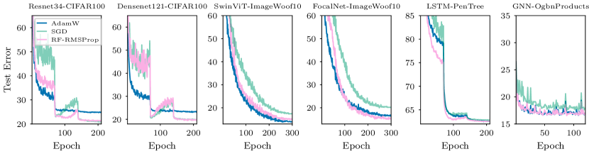
Figure 1: In modern training setups (learning rate schedule, random search), square-root-free (RF) adaptive methods close the generalization gap between their root-based counterparts and SGD on CNNs (CIFAR-100), while maintaining their performance on vision transformers (ImageWoof10). They also work well on other problems, like training a 3-layer LSTM and a GNN (Zhang et al., 2022).

Adaptive gradient-based methods like Adam (Kingma & Ba, 2015) play a significant role in training modern deep learning models such as transformers. A better understanding of these methods allows us to address their shortcomings and develop new adaptive methods to reduce training time and improve performance. This is essential as deep learning models become increasingly large and complex to train.

Despite their success on architectures like transformers, adaptive methods tend to generalize worse than stochastic gradient descent (SGD) on convolutional architectures (Wilson et al., 2017). Our understanding of this discrepancy is limited. Balles & Hennig (2018) dissect Adam into two concepts, sign descent and adaptive step sizes, and hypothesize that the connection to sign descent could cause the generalization gap with SGD on CNNs. Similarly, Kunstner et al. (2023); Chen et al. (2023) argue that adaptive methods outperform SGD on transformers due to their connection to sign descent.

It is challenging to isolate the sign descent component of adaptive methods like Adam or RMSProp (Tieleman & Hinton, 2012), as they typically introduce a square root to the preconditioner, which conflates the sign and adaptivity aspects. The root is motivated by reports of improved performance (Tieleman & Hinton, 2012) and to stabilize convergence near the optimum (Kingma & Ba, 2015; Kunstner et al., 2019; Martens, 2020). However, it conflicts with the motivation of adaptive methods as approximate second-order methods based on the empirical Fisher, which is also commonly mentioned in works introducing adaptive methods (e.g. Kingma & Ba, 2015).

Here, we investigate how the behavior of adaptive methods changes when we remove the root. Our idea is to strengthen their often-mentioned link to second-order methods that is weakened by the root. Conceptually, this cleanly disentangles the aforementioned adaptivity aspect from the sign aspect. Practically, it provides an opportunity to revisit the root’s role in the context of modern training strategies, such as using non-constant learning rate schedules (Loshchilov & Hutter, 2016) and hyperparameter tuning schemes (Choi et al., 2019), that differ from the original pipelines in which the square root was introduced. Computationally, removing the root is beneficial for lowering memory consumption and per-iteration cost of non-diagonal matrix adaptive methods, which require costly matrix decompositions that need to be carried out in high precision to avoid numerical instabilities (Gupta et al., 2018; Anil et al., 2020).

There are some challenges to establishing a rigorous second-order perspective on adaptive methods; one cannot just remove the root. We overcome those challenges and make the following contributions:

• We establish a rigorous second-order view of adaptive methods: we remove the square root (Section 2), show how to interpret the gradient outer product as a new empirical Fisher variant (Section 3), and adjust the preconditioner initialization (Section 4).

• Empirically, we show that—surprisingly—removing the root not only closes the generalization gap between adaptive methods and SGD on convolutional neural networks, but maintains the performance of root-based methods on vision transformers (Section 2).

• We demonstrate the second-order perspective’s conceptual and computational merits to develop matrix adaptive methods that, thanks to recent approaches on inverse-free second-order methods (Lin et al., 2023), require neither matrix inverses nor matrix square roots and can therefore run in low precision—a crucial ingredient for modern training (Section 4).

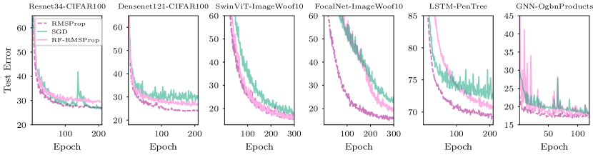
Figure 2: Comparison of root-based versus square-root-free (RF) methods in the original (outdated) training setup the square root was introduced in. Adaptive methods with square root work better than their square root free counterparts when using (1) a constant learning rate schedule, (2) default zero initialization, (3) default scaling.

2 First-order View of Adaptive Methods

For many deep learning tasks, training a neural network (NN) means solving an unconstrained optimization problem. For simplicity, consider a supervised learning task with a set of $N$ data points $\{y_{i},\mbox{$\mbox{$\mathbf{x}$}$}_{i}\}_{i=1}^{N}$, where $y_{i}$ and $\mbox{$\mbox{$\mathbf{x}$}$}_{i}$ represent a label and a feature vector. Given a NN $f(\cdot;\mbox{$\mbox{$\boldsymbol{\mu}$}$})$ with learnable weights $\boldsymbol{\mu}$, the optimization problem is

$$\min_{\mu}\ell(\mbox{$\mbox{$\boldsymbol{\mu}$}$}):=\sum_{i=1}^{N}c(y_{i},f(\mbox{$\mbox{$\mathbf{x}$}$}_{i};\mbox{$\mbox{$\boldsymbol{\mu}$}$})),$$ (1)

where $\hat{y}_{i}:=f(\mbox{$\mbox{$\mathbf{x}$}$}_{i};\mbox{$\mbox{$\boldsymbol{\mu}$}$})$ is a predicted label given a feature vector $\mbox{$\mbox{$\mathbf{x}$}$}_{i}$ as an input to the NN and $c(y_{i},\hat{y}_{i})$ is a loss function that measures a discrepancy between the true ($y_{i}$) and predicted ($\hat{y}_{i}$) label.

To solve this optimization problem, we can use adaptive gradient methods, which use the following preconditioned gradient update

$$\mbox{$\mbox{$\boldsymbol{\mu}$}$}\leftarrow\mbox{$\mbox{$\boldsymbol{\mu}$}$}-\beta_{1}\mbox{$\mbox{$\mathbf{S}$}$}^{-1}\nabla_{\mu}\ell(\mbox{$\mbox{$\boldsymbol{\mu}$}$}),$$ (2)

where $\beta_{1}$ is a (initial) learning rate, $\nabla_{\mu}\ell(\mbox{$\mbox{$\boldsymbol{\mu}$}$})$ is a gradient vector, and $\mathbf{S}$ is a preconditioning matrix. When $\mathbf{S}$ is the Hessian and $\beta_{1}=1$, this becomes Newton’s method. In adaptive gradient methods, the preconditioning matrix $\mathbf{S}$ is estimated by using only gradient information.

To estimate the preconditioner $\mathbf{S}$, most adaptive methods employ an outer product $\mbox{$\mbox{$\mathbf{H}$}$}:=\mbox{$\mbox{$\mathbf{g}$}$}\mbox{$\mbox{$\mathbf{g}$}$}^{T}$ of a gradient vector $\mathbf{g}$ that is usually the mini-batch gradient of Equation 1: Diagonal adaptive methods such as RMSProp (Tieleman & Hinton, 2012), AdaGrad (Duchi et al., 2011), and Adam (Kingma & Ba, 2015), only use the diagonal entries $\mathrm{diag}(\mbox{$\mbox{$\mathbf{H}$}$})=\mbox{$\mbox{$\mathbf{g}$}$}\odot\mbox{$\mbox{$\mathbf{g}$}$}$ where $\odot$ denotes element-wise multiplication. Full matrix adaptive methods like AdaGrad (Duchi et al., 2011) and its variants (Agarwal et al., 2019) use the gradient outer product $\mathbf{H}$. Structured matrix methods like Shampoo (Gupta et al., 2018) use a Kronecker-factored approximation of the gradient outer product $\mathbf{H}$.

All of these methods apply a square root to the preconditioner in their update, and we will refer to them as square root based methods. For example, RMSProp updates its preconditioner $\mbox{$\mbox{$\mathbf{S}$}$}=\mathrm{diag}(\sqrt{\hat{\mbox{$\mbox{$\mathbf{s}$}$}}})$ and parameters according to

where $\mbox{$\mbox{$\mathbf{h}$}$}:=\mathrm{diag}(\mbox{$\mbox{$\mathbf{H}$}$})$, $\beta_{1}$ is the learning rate, and $\beta_{2}$ is the weight to incorporate new outer products. In full-matrix cases, adding the root requires matrix root decomposition. For example, full-matrix AdaGrad updates its preconditioner $\mbox{$\mbox{$\mathbf{S}$}$}=\hat{\mbox{$\mbox{$\mathbf{S}$}$}}^{\frac{1}{2}}$ and parameters as

$$\hat{\mbox{$\mbox{$\mathbf{S}$}$}}\leftarrow\hat{\mbox{$\mbox{$\mathbf{S}$}$}}+\beta_{2}\mbox{$\mbox{$\mathbf{g}$}$}\mbox{$\mbox{$\mathbf{g}$}$}^{T},\,\mbox{$\mbox{$\boldsymbol{\mu}$}$}\leftarrow\mbox{$\mbox{$\boldsymbol{\mu}$}$}-\beta_{1}\mbox{$\mbox{$\mathbf{S}$}$}^{-1}\mbox{$\mbox{$\mathbf{g}$}$}.$$ (4)

We have to use a symmetric square-root decomposition $\hat{\mbox{$\mbox{$\mathbf{S}$}$}}^{\frac{1}{2}}$ to compute the preconditioner.

2.1 Benefits and Results of Removing the Square Root

It is unclear how exactly the square root emerged in adaptive methods. Here, we hypothesize how it got introduced, critically assess why it may be desirable to remove, and highlight connections to our experimental results. We find that few works study square-root-free adaptive methods, and the benefits of removing the root are often overlooked in the literature. Our work fills in this gap, which we think is crucial to better understand these methods and our empirical results underline the great potential of square-root-free adaptive methods.

Empirical performance & training schemes

The most important motivation in favor of the square root is the strong empirical performance of square-root-based methods that has been demonstrated in various works and rightfully established them as state-of-the-art for training transformers. However, the context in which the root was introduced significantly differed from the training schemes that are used nowadays. Original works such as Tieleman & Hinton (2012) show that including the square root improves the performance of adaptive methods when only tuning a learning rate that is fixed throughout training (Bottou et al., 2018). Beyond this original setting, square-root-based methods have demonstrated great capabilities to train a wide range of NNs, e.g. when using a non-constant learning rate (Loshchilov & Hutter, 2016) and random search (Bergstra & Bengio, 2012; Choi et al., 2019) to tune all available hyper-parameters. We wonder whether the square root, while necessary to achieve good performance in outdated training schemes, might not be required in contemporary schemes. To investigate this hypothesis, we conducted an experiment that compares square-root-based and square-root-free methods using the original training scheme in which the square root was introduced (Figure 2). Indeed, we find that the square root is beneficial in this context.

Interpretability & generalization

Square-root-based methods are state-of-the-art for training attention-based models, but exhibit a generalization gap with SGD on CNNs (Wilson et al., 2017). The square root complicates the understanding of this phenomenon. Recent studies attribute the superior performance of adaptive methods over SGD on attention models to their sign-based update rules (Kunstner et al., 2023; Chen et al., 2023). Balles & Hennig (2018) hypothesize that sign descent may cause poor generalization of Adam on CNNs. However, they neither consider the direct effect of the square root nor remove it from an existing method. Therefore, the role of adaptivity as another main factor behind the performance gap is unclear since adding the root conflates sign descent and adaptivity. Removing the square root could clarify this issue, as a square-root-free method no longer performs sign descent. To investigate the role of adaptivity, we experiment with square-root-free RMSProp (Figure 4) on attention and convolutional models (Figure 1). For transformer-based architectures, we find that removing the square root does not negatively affect the performance of RMSProp. This suggests that not only sign descent, but also adaptivity, might be a key factor behind the performance gap between adaptive methods and SGD on transformers. For convolutional architectures, removing the square root closes the generalization gap between RMSProp and SGD. This suggests that square-root-free adaptive methods can generalize well, and raises novel questions on the understanding of the role of adaptivity.

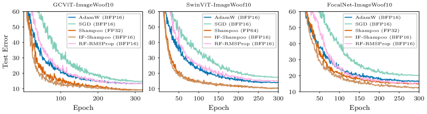
Figure 3: Comparison of matrix adaptive square-root-free versus square-root-based methods. Both matrix adaptive methods (Shampoo, IF-Shampoo) outperform diagonal adaptive methods on vision transformers using modern training strategies. In contrast to Shampoo, our inverse-free matrix adaptive method, IF-Shampoo, runs in BFP-16 and trains roughly twice as fast, while using less memory.

Computational cost

As noted by Duchi et al. (2011), the square root poses numerical and computational challenges on matrix adaptive methods like Equation 4 as it requires matrix square roots which must be carried out in high precision, to avoid numerical instabilities. This increases the run time, memory footprint, and complicates the implementation (Anil et al., 2020; Shi et al., 2023). Using low-precision data types (Micikevicius et al., 2017) is a key technique to boost training speed and reduce memory. The use of the square root makes these matrix methods undesirable for modern low-precision training schemes. By removing the square root, and using the latest advances on second-order methods (Lin et al., 2023), we can develop inverse-free matrix adaptive methods (Section 4.3) that are suitable for mixed-precision training. We present empirical results for the low-precision setting in Figure 3. Thanks to removing the square root, we can consistently train in BFP-16, whereas square-root-based adaptive matrix methods like Shampoo need single—in some cases, even double—precision. On modern vision transformers, we find that adaptive matrix methods outperform diagonal adaptive methods and perform similarly to Shampoo while requiring less time due to mixed-precision training. This shows that removing the square root allows us to overcome the challenges of existing matrix adaptive methods and expand their applicability to modern training pipelines.

Theoretical considerations

Invariances. Adding the square root makes a descent step invariant to the scale of the loss – the square root adjusts the scale of the “squared” gradient to be consistent with the gradient when the loss function is scaled. This is useful as there is no need for users to pay attention to whether the loss function is averaged or summed over data points. While adding the square root fixes the scaling issue, it breaks the affine reparameterization invariance (Nesterov & Nemirovskii, 1994). We can fix the scaling issue and preserve the affine invariance without the square root, as will be shown in Section 3; see Appendix A for an example of the affine invariance of square-root-free methods.

Convergence analysis. Theoretical works such as Duchi et al. (2011); Reddi et al. (2019) and many others suggest that adding the square root is useful to prove convergence bounds for convex loss functions. Convergence analysis for square-root-based methods is also extended to non-convex settings when certain assumptions such as gradient Lipschitz and Polyak-Łojasiewicz condition are satisfied. However, compared to the regret bound of AdaGrad (Duchi et al., 2011) studied in convex settings, Hazan et al. (2006) give a better regret bound in strongly-convex cases without introducing the square root. Recent works such as Mukkamala & Hein (2017); Wang et al. (2020) prove similar bounds for square-root-free methods for convex problems. Thus, square-root-free methods are theoretically grounded—at least in convex settings.

Behavior near optimum. The square root is often introduced to avoid oscillation near an optimal solution where the preconditioner can be ill-conditioned. For example, in one dimension when near the optimum, the descent direction $s^{-1}g$ can be unbounded when we use the outer product as the preconditioner $s=g^{2}$ because the gradient $g$ is close to $0$ at the optimum and the outer product as a ‘squared’ gradient decreases much faster than the gradient $g$. Thus, the update without the square root can lead to oscillation when using a constant learning rate. However, even without the square root, a preconditioner can still be well-conditioned when incorporating outer products from previous iterations (Roux et al., 2007) and using Tikhonov damping (Becker et al., 1988; Martens & Sutskever, 2012). For example, the descent direction $s^{-1}g$ can be bounded without the square root even when near an optimal solution, where $g$ is a gradient and $s=(1-\beta_{2})s+\beta_{2}g^{2}$ is a preconditioner estimated by an exponentially moving average.

RMSProp 1:  Compute gradient $\mbox{$\mbox{$\mathbf{g}$}$}:=\nabla\ell_{\text{scaled}}(\mbox{$\mbox{$\boldsymbol{\mu}$}$})$ $\hat{\mbox{$\mbox{$\mathbf{s}$}$}}\leftarrow(1-\beta_{2})\hat{\mbox{$\mbox{$\mathbf{s}$}$}}+\beta_{2}\mbox{$\mbox{$\mathbf{g}$}$}^{2}$ 2:   $\mbox{$\mbox{$\boldsymbol{\mu}$}$}\leftarrow\mbox{$\mbox{$\boldsymbol{\mu}$}$}-\beta_{1}\mbox{$\mbox{$\mathbf{g}$}$}/\sqrt{\hat{\mbox{$\mbox{$\mathbf{s}$}$}}}$ Square-root-free RMSProp (Ours) 1:  Compute gradient $\mbox{$\mbox{$\mathbf{g}$}$}:=\nabla\ell_{\text{scaled}}(\mbox{$\mbox{$\boldsymbol{\mu}$}$})$ $\mbox{$\mbox{$\mathbf{s}$}$}\leftarrow(1-\beta_{2})\mbox{$\mbox{$\mathbf{s}$}$}+\beta_{2}{\color[rgb]{1,0,0}\mbox{$\mbox{$\mathbf{B}$}$}}\mbox{$\mbox{$\mathbf{g}$}$}^{2}$ 2:   $\mbox{$\mbox{$\boldsymbol{\mu}$}$}\leftarrow\mbox{$\mbox{$\boldsymbol{\mu}$}$}-\beta_{1}\mbox{$\mbox{$\mathbf{g}$}$}/\mbox{$\mbox{$\mathbf{s}$}$}$

Figure 4: Diagonal adaptive methods for a (scaled) loss function $\ell_{\text{scaled}}(\mbox{$\mbox{$\boldsymbol{\mu}$}$})$ defined by averaging over $B$ data points. We initialize $s$ to $1$ in the square-free method in our square-root-free method while $\hat{s}$ is initialized to $0$ in the original RMSProp. For simplicity, we do not include damping, weight decay, and momentum. A full-fledged version can be found in the Appendix, Figure 6.

3 A Second-order Perspective

Here, we describe a second-order perspective on adaptive methods without the square root. This naturally resolves the scaling issue and is coherent with the original motivation to develop these methods.

Without the square root, an adaptive method takes a step

$$\mbox{$\mbox{$\mathbf{S}$}$}\leftarrow(1-\beta_{2}\gamma)\mbox{$\mbox{$\mathbf{S}$}$}+\beta_{2}\mbox{$\mbox{$\mathbf{H}$}$},\qquad\mbox{$\mbox{$\boldsymbol{\mu}$}$}\leftarrow\mbox{$\mbox{$\boldsymbol{\mu}$}$}-\beta_{1}\mbox{$\mbox{$\mathbf{S}$}$}^{-1}\mbox{$\mbox{$\mathbf{g}$}$},$$ (5)

where the outer product $\mbox{$\mbox{$\mathbf{H}$}$}=\mbox{$\mbox{$\mathbf{g}$}$}\mbox{$\mbox{$\mathbf{g}$}$}^{T}$ is used as a curvature approximation. For example, when $\gamma=0$ and $\mathbf{S}$ is a full matrix, we obtain the update of full-matrix AdaGrad without the square root.

The above update resembles a second-order method. However, it is not invariant to the scale of the loss, unlike Newton’s method: Scaling the loss by a constant $c$ scales the gradient and Hessian by $c$, but the gradient outer product by $c^{2}$, which is inconsistent with its role as a Hessian approximation and therefore conflicts with the second-order interpretation. We will resolve this particular conflict and improve the justification of square-root-free adaptive methods through approximate second-order methods.

The key step is to define the gradient outer product as a novel empirical Fisher that differs from the standard empirical Fisher discussed in the deep learning literature (Kingma & Ba, 2015; Kunstner et al., 2019; Martens, 2020). Our empirical Fisher relies on the aggregated mini-batch gradient, rather than per-sample gradients. Since the Fisher is tied to a probability distribution that must be normalized, this provides a gauge to automatically make updates invariant to the scale of the loss.

3.1 A New Empirical Fisher as a Hessian Approximation

Recall that the objective function $\ell(\mbox{$\mbox{$\boldsymbol{\mu}$}$})=\sum_{i=1}^{N}c(y_{i},f(\mbox{$\mbox{$\mathbf{x}$}$}_{i};\mbox{$\mbox{$\boldsymbol{\mu}$}$}))$ is defined in (1). Given data point $\mbox{$\mbox{$\mathbf{x}$}$}_{i}$, we can define a per-example probability distribution over label $y_{i}$ as $p(y_{i}|\mbox{$\mbox{$\mathbf{x}$}$}_{i};\mbox{$\mbox{$\boldsymbol{\mu}$}$})=\exp(-c(y_{i},f(\mbox{$\mbox{$\mathbf{x}$}$}_{i};\mbox{$\mbox{$\boldsymbol{\mu}$}$})))$ by using the loss function $c(y_{i},f(\mbox{$\mbox{$\mathbf{x}$}$}_{i};\mbox{$\mbox{$\boldsymbol{\mu}$}$}))$ (e.g., cross-entropy loss, square loss). We denote an individual or per-example gradient for data point $\mbox{$\mbox{$\mathbf{x}$}$}_{i}$ by $\mbox{$\mbox{$\mathbf{g}$}$}_{i}:=\nabla_{\mu}c(y_{i},f(\mbox{$\mbox{$\mathbf{x}$}$}_{i};\mbox{$\mbox{$\boldsymbol{\mu}$}$}))=-\nabla_{\mu}\log p(y_{i}|\mbox{$\mbox{$\mathbf{x}$}$}_{i};\mbox{$\mbox{$\boldsymbol{\mu}$}$})$ .

(1) Standard empirical Fisher matrices

Definition 1.

The empirical Fisher information (FIM) matrix (Kingma & Ba, 2015; Kunstner et al., 2019; Martens, 2020) $\tilde{\mbox{$\mbox{$\mathbf{F}$}$}}_{\text{standard}}(\mbox{$\mbox{$\boldsymbol{\mu}$}$})$ is defined by replacing the expectation in the standard FIM $\mbox{$\mbox{$\mathbf{F}$}$}_{\text{standard}}(\mbox{$\mbox{$\boldsymbol{\mu}$}$})$ with observed labels.

Now we introduce a new Fisher matrix as a FIM over a joint distribution of the labels.

(2) Our Fisher matrices for the original (unscaled) loss

Definition 2.

Our Fisher matrix is defined as

where the labels $\mbox{$\mbox{$\mathbf{y}$}$}=(y_{1},\cdots,y_{N})$ are considered jointly as a random vector, $p(\mbox{$\mbox{$\mathbf{y}$}$}|\mbox{$\mbox{$\mathbf{X}$}$};\mbox{$\mbox{$\boldsymbol{\mu}$}$}):=\prod_{i=1}^{N}p(y_{i}|\mbox{$\mbox{$\mathbf{x}$}$}_{i};\mbox{$\mbox{$\boldsymbol{\mu}$}$})$ is its joint distribution, and $\mbox{$\mbox{$\mathbf{X}$}$}=(\mbox{$\mbox{$\mathbf{x}$}$}_{1},\cdots,\mbox{$\mbox{$\mathbf{x}$}$}_{N})$ is a feature matrix.

Definition 3.

Our empirical Fisher matrix is defined by replacing the expectation in $\mbox{$\mbox{$\mathbf{F}$}$}_{\text{new}}(\mbox{$\mbox{$\boldsymbol{\mu}$}$})$ with observed labels.

where $\nabla_{\mu}\log p(\mbox{$\mbox{$\mathbf{y}$}$}|\mbox{$\mbox{$\mathbf{X}$}$};\mbox{$\mbox{$\boldsymbol{\mu}$}$})=\sum_{i=1}^{N}\nabla_{\mu}\log p(y_{i}|\mbox{$\mbox{$\mathbf{x}$}$}_{i};\mbox{$\mbox{$\boldsymbol{\mu}$}$})=-\sum_{i=1}^{N}\mbox{$\mbox{$\mathbf{g}$}$}_{i}=-\mbox{$\mbox{$\mathbf{g}$}$}$ .

According to (7), we can see that the outer product $\mbox{$\mbox{$\mathbf{H}$}$}=\mbox{$\mbox{$\mathbf{g}$}$}\mbox{$\mbox{$\mathbf{g}$}$}^{T}$ coincides with this empirical Fisher matrix $\tilde{\mbox{$\mbox{$\mathbf{F}$}$}}_{\text{new}}(\mbox{$\mbox{$\boldsymbol{\mu}$}$})$.

Definition 4.

In a mini-batch case, we can define a Fisher matrix for a mini-batch with $B$ data points as

where $\mbox{$\mbox{$\mathbf{y}$}$}_{\text{mini}}:=(y_{1},\cdots,y_{B})$ is a label vector, $\mbox{$\mbox{$\mathbf{X}$}$}_{\text{mini}}:=(\mbox{$\mbox{$\mathbf{x}$}$}_{1},\cdots,\mbox{$\mbox{$\mathbf{x}$}$}_{B})$ is a feature matrix for the mini-batch, and $p(\mbox{$\mbox{$\mathbf{y}$}$}_{\text{mini}}|\mbox{$\mbox{$\mathbf{X}$}$}_{\text{mini}};\mbox{$\mbox{$\boldsymbol{\mu}$}$}):=\prod_{i=1}^{B}p(y_{i}|\mbox{$\mbox{$\mathbf{x}$}$}_{i},\mbox{$\mbox{$\boldsymbol{\mu}$}$})$ is the joint distribution over labels for the mini-batch. This distribution can also be obtained by marginalizing unseen labels in the original joint distribution $p(\mbox{$\mbox{$\mathbf{y}$}$}|\mbox{$\mbox{$\mathbf{X}$}$};\mbox{$\mbox{$\boldsymbol{\mu}$}$})$ defined for the full-batch.

This Fisher is an unbiased estimation of our full-batch Fisher as the claim—proof in Appendix B—is stated below.

Claim 1.

Our mini-batch Fisher $\frac{1}{B}\mbox{$\mbox{$\mathbf{F}$}$}_{\text{mini}}(\mbox{$\mbox{$\boldsymbol{\mu}$}$})$ is an unbiased estimation of the full-batch Fisher $\frac{1}{N}\mbox{$\mbox{$\mathbf{F}$}$}_{\text{new}}(\mbox{$\mbox{$\boldsymbol{\mu}$}$})$.

When we replace the expectation with observed labels, we obtain our empirical Fisher for the mini-batch. Note that this empirical Fisher is not an unbiased estimator of the full-batch empirical Fisher. However, we often do not consider the unbiasedness when we incorporate empirical Fisher matrices from previous iterations. For example, consider the update of AdaGrad. Moreover, our interpretation provides the direct link to the Hessian as we can view the outer product as a Hessian approximation (see (7)) when the product corresponds to our Fisher. This interpretation allows us to preserve the scale-invariance to the loss and the affine reparametrization invariance in square-root-free methods.

(3) Our Fisher matrices for a scaled loss

Now, we consider a case when the loss function is scaled. In this case, the outer product $\mathbf{H}$ no longer coincides with a Fisher matrix. As an example, we consider averaging a loss over $N>1$ data points, as it is often done in mini-batch settings. The loss is

where the gradient and the outer product are defined as $\mbox{$\mbox{$\mathbf{g}$}$}_{\text{scaled}}:=\frac{1}{N}\sum_{i=1}^{N}\nabla_{\mu}c(y_{i},f(\mbox{$\mbox{$\mathbf{x}$}$}_{i};\mbox{$\mbox{$\boldsymbol{\mu}$}$}))=\frac{1}{N}\sum_{i=1}^{N}\mbox{$\mbox{$\mathbf{g}$}$}_{i}$ and $\mbox{$\mbox{$\mathbf{H}$}$}_{\text{scaled}}:=\mbox{$\mbox{$\mathbf{g}$}$}_{\text{scaled}}\mbox{$\mbox{$\mathbf{g}$}$}_{\text{scaled}}^{T}=\frac{1}{N^{2}}\mbox{$\mbox{$\mathbf{H}$}$}$ , respectively.

In this case, the empirical Fisher matrix should be defined using the same joint distribution as

According to (9), the outer product $\mbox{$\mbox{$\mathbf{H}$}$}_{\text{scaled}}$ no longer coincides with this empirical Fisher matrix $\tilde{\mbox{$\mbox{$\mathbf{F}$}$}}_{\text{scaled}}(\mbox{$\mbox{$\boldsymbol{\mu}$}$})$. When using $\tilde{\mbox{$\mbox{$\mathbf{F}$}$}}_{\text{scaled}}(\mbox{$\mbox{$\boldsymbol{\mu}$}$})$ as the Hessian approximation, the update of a square-root-free adaptive method is

Observe that the above update is scale invariant since the gradient $\mbox{$\mbox{$\mathbf{g}$}$}_{\text{scaled}}=\frac{1}{N}\mbox{$\mbox{$\mathbf{g}$}$}$ and this empirical Fisher $\tilde{\mbox{$\mbox{$\mathbf{F}$}$}}_{\text{scaled}}(\mbox{$\mbox{$\boldsymbol{\mu}$}$})=N\mbox{$\mbox{$\mathbf{H}$}$}_{\text{scaled}}=\frac{1}{N}\mbox{$\mbox{$\mathbf{H}$}$}$ have the same scale.

Affine reparametrization invariance

Our fix does not break the affine invariance of a square-root-free method. A square-root-free method is affine invariant when using our scaled empirical Fisher matrix as shown in Claim 2 (see Appx. C for a proof).

Claim 2.

Our square-root-free update is affine invariant.

By using our empirical Fisher matrices, our square-root-free methods like Newton’s method not only is scale-invariant when we scale a loss function but also preserves the affine reparametrization invariance. Thus, we consider our methods as approximate second-order methods.

3.2 Difference to the Standard Empirical Fisher

Existing works (Kingma & Ba, 2015; Kunstner et al., 2019; Martens, 2020) do not distinguish the standard empirical Fisher denoted by $\tilde{\mbox{$\mbox{$\mathbf{F}$}$}}_{\text{standard}}(\mbox{$\mbox{$\boldsymbol{\mu}$}$})$ from the outer product $\mathbf{H}$ corresponding to our empirical Fisher $\tilde{\mbox{$\mbox{$\mathbf{F}$}$}}_{\text{new}}(\mbox{$\mbox{$\boldsymbol{\mu}$}$})$ . They are different when $N>1$ since

From the above equation, we can see that the standard empirical Fisher on the left is not a rank-one matrix while our empirical Fisher on the right is a rank-one matrix.

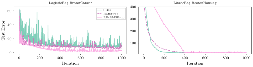
Figure 8: Experiments demonstrating that square-root-free adaptive methods work well in stochastic convex settings, where we train the models using mini-batches.

This misconception can impede our understanding of these methods. The outer product $\mathbf{H}$ corresponding to our empirical Fisher $\tilde{\mbox{$\mbox{$\mathbf{F}$}$}}_{\text{new}}(\mbox{$\mbox{$\boldsymbol{\mu}$}$})$ is different from the standard empirical Fisher considered by Kunstner et al. (2019). Indeed, some limitations in Kunstner et al. (2019) are due to the ill-conditioning issue near optimum as discussed in Sec. 2. Importantly, we estimate a preconditioner $\mathbf{S}$ and overcome the ill-conditioning issue by incorporating outer products from previous iterations (e.g., by a moving average) – even in the full-batch setting as shown in (5). Aggregating these previous outer products makes our approximation distinct from the approximation considered by Kunstner et al. (2019) where the authors do not make use of previous products. As shown in Fig. 8 in Appendix E, our estimation works well in the examples considered by Kunstner et al. (2019). Furthermore, our approximation has been theoretically justified (Hazan et al., 2006; Mukkamala & Hein, 2017; Wang et al., 2020) for square-root-free methods in (convex) settings similar to Kunstner et al. (2019). Thus, our empirical Fisher does not suffer from all the limitations of the standard empirical Fisher discussed in Kunstner et al. (2019) when using our Fisher in the preconditioner estimation.

3.3 Disentangling the Outer Product from the Fisher

At first glance, in the scaled case the outer product $\mbox{$\mbox{$\mathbf{H}$}$}_{\text{scaled}}$ coincides with an empirical Fisher $\tilde{{\mbox{$\mbox{$\mathbf{F}$}$}}}_{\text{incorrect}}(\mbox{$\mbox{$\boldsymbol{\mu}$}$})=\nabla_{\mu}\log p_{\text{scaled}}(\mbox{$\mbox{$\mathbf{y}$}$}|\mbox{$\mbox{$\mathbf{X}$}$};\mbox{$\mbox{$\boldsymbol{\mu}$}$})\nabla_{\mu}^{\top}\log p_{\text{scaled}}(\mbox{$\mbox{$\mathbf{y}$}$}|\mbox{$\mbox{$\mathbf{X}$}$};\mbox{$\mbox{$\boldsymbol{\mu}$}$})$ . This empirical Fisher is defined over a different joint distribution $p_{\text{scaled}}(\mbox{$\mbox{$\mathbf{y}$}$}|\mbox{$\mbox{$\mathbf{X}$}$};\mbox{$\mbox{$\boldsymbol{\mu}$}$})=\prod_{i=1}^{N}p_{\text{scaled}}(y_{i}|\mbox{$\mbox{$\mathbf{x}$}$}_{i};\mbox{$\mbox{$\boldsymbol{\mu}$}$})$ and depends on a scaled per-sample probability distribution over label $y_{i}$ as $p_{\text{scaled}}(y_{i}|\mbox{$\mbox{$\mathbf{x}$}$}_{i};\mbox{$\mbox{$\boldsymbol{\mu}$}$})=\exp(-{\color[rgb]{1,0,0}\frac{1}{N}}c(y_{i},f(\mbox{$\mbox{$\mathbf{x}$}$}_{i};\mbox{$\mbox{$\boldsymbol{\mu}$}$})))$ . However, this scaled distribution cannot be normalized. Therefore, we cannot define a valid Fisher that corresponds to the outer product. In other words, the product is not necessary an empirical Fisher matrix. The normalization condition of a per-sample distribution is often overlooked in the literature when considering a gradient outer product as an empirical Fisher.

Shampoo 1:  Compute $\mbox{$\mbox{$\mathbf{G}$}$}:=\mathrm{Mat}(\nabla\ell_{\text{scaled}}(\mbox{$\mbox{$\boldsymbol{\mu}$}$}))$ $\hat{\mbox{$\mbox{$\mathbf{S}$}$}}_{C}\leftarrow(1-\beta_{2}\gamma)\hat{\mbox{$\mbox{$\mathbf{S}$}$}}_{C}+\beta_{2}\mbox{$\mbox{$\mathbf{G}$}$}\mbox{$\mbox{$\mathbf{G}$}$}^{T}$ $\hat{\mbox{$\mbox{$\mathbf{S}$}$}}_{K}\leftarrow(1-\beta_{2}\gamma)\hat{\mbox{$\mbox{$\mathbf{S}$}$}}_{K}+\beta_{2}\mbox{$\mbox{$\mathbf{G}$}$}^{T}\mbox{$\mbox{$\mathbf{G}$}$}$ 2:   $\mathrm{Mat}(\mbox{$\mbox{$\boldsymbol{\mu}$}$})\leftarrow\mathrm{Mat}(\mbox{$\mbox{$\boldsymbol{\mu}$}$})-\beta_{1}\hat{\mbox{$\mbox{$\mathbf{S}$}$}}_{C}^{-1/4}\mbox{$\mbox{$\mathbf{G}$}$}\hat{\mbox{$\mbox{$\mathbf{S}$}$}}_{K}^{-1/4}$ Square-root-free Shampoo (Ours) 1:  Compute $\mbox{$\mbox{$\mathbf{G}$}$}:=\mathrm{Mat}(\nabla\ell_{\text{scaled}}(\mbox{$\mbox{$\boldsymbol{\mu}$}$}))$ $\mbox{$\mbox{$\mathbf{S}$}$}_{C}\leftarrow(1-\beta_{2}\gamma)\mbox{$\mbox{$\mathbf{S}$}$}_{C}+\frac{\beta_{2}}{d}({\color[rgb]{1,0,0}B}\mbox{$\mbox{$\mathbf{G}$}$}\mbox{$\mbox{$\mathbf{S}$}$}_{K}^{-1}\mbox{$\mbox{$\mathbf{G}$}$}^{T})$ $\mbox{$\mbox{$\mathbf{S}$}$}_{K}\leftarrow(1-\beta_{2}\gamma)\mbox{$\mbox{$\mathbf{S}$}$}_{K}+\frac{\beta_{2}}{p}({\color[rgb]{1,0,0}B}\mbox{$\mbox{$\mathbf{G}$}$}^{T}\mbox{$\mbox{$\mathbf{S}$}$}_{C}^{-1}\mbox{$\mbox{$\mathbf{G}$}$})$ 2:   $\mathrm{Mat}(\mbox{$\mbox{$\boldsymbol{\mu}$}$})\leftarrow\mathrm{Mat}(\mbox{$\mbox{$\boldsymbol{\mu}$}$})-\beta_{1}\mbox{$\mbox{$\mathbf{S}$}$}_{C}^{-1}\mbox{$\mbox{$\mathbf{G}$}$}\mbox{$\mbox{$\mathbf{S}$}$}_{K}^{-1}$ Inverse-free Shampoo (Ours) 1:  Compute $\mbox{$\mbox{$\mathbf{G}$}$}:=\mathrm{Mat}(\nabla\ell_{\text{scaled}}(\mbox{$\mbox{$\boldsymbol{\mu}$}$}))$ ${\mbox{$\mbox{$\mathbf{C}$}$}}\leftarrow{\mbox{$\mbox{$\mathbf{C}$}$}}\exp(-\frac{\beta_{2}}{2d}({\color[rgb]{1,0,0}B}{\mbox{$\mbox{$\mathbf{C}$}$}}^{T}\mbox{$\mbox{$\mathbf{G}$}$}{\mbox{$\mbox{$\mathbf{K}$}$}}{\mbox{$\mbox{$\mathbf{K}$}$}}^{T}\mbox{$\mbox{$\mathbf{G}$}$}^{T}{\mbox{$\mbox{$\mathbf{C}$}$}}-\gamma d\mbox{$\mbox{$\mathbf{I}$}$}))$ ${\mbox{$\mbox{$\mathbf{K}$}$}}\leftarrow{\mbox{$\mbox{$\mathbf{K}$}$}}\exp(-\frac{\beta_{2}}{2p}({\color[rgb]{1,0,0}B}\bar{\mbox{$\mbox{$\mathbf{K}$}$}}^{T}\mbox{$\mbox{$\mathbf{G}$}$}^{T}{\mbox{$\mbox{$\mathbf{C}$}$}}{\mbox{$\mbox{$\mathbf{C}$}$}}^{T}\mbox{$\mbox{$\mathbf{G}$}$}{\mbox{$\mbox{$\mathbf{K}$}$}}-\gamma p\mbox{$\mbox{$\mathbf{I}$}$}))$ 2:   $\mathrm{Mat}(\mbox{$\mbox{$\boldsymbol{\mu}$}$})\leftarrow\mathrm{Mat}(\mbox{$\mbox{$\boldsymbol{\mu}$}$})-\beta_{1}{\mbox{$\mbox{$\mathbf{C}$}$}}{\mbox{$\mbox{$\mathbf{C}$}$}}^{T}\mbox{$\mbox{$\mathbf{G}$}$}{\mbox{$\mbox{$\mathbf{K}$}$}}{\mbox{$\mbox{$\mathbf{K}$}$}}^{T}$

Figure 5: Structured matrix adaptive methods for a (scaled) loss function $\ell_{\text{scaled}}(\mbox{$\mbox{$\boldsymbol{\mu}$}$})$ defined by averaging over $B$ data points. For simplicity, we assume $\mathrm{Mat}(\mbox{$\mbox{$\boldsymbol{\mu}$}$})\in\mathcal{R}^{p\times d}$ is a weight matrix in a layer. $\hat{\mbox{$\mbox{$\mathbf{S}$}$}}_{C},\mbox{$\mbox{$\mathbf{S}$}$}_{C},\mbox{$\mbox{$\mathbf{C}$}$}\in^{p\times p}$ and $\hat{\mbox{$\mbox{$\mathbf{S}$}$}}_{K},\mbox{$\mbox{$\mathbf{S}$}$}_{K},\mbox{$\mbox{$\mathbf{K}$}$}\in^{d\times d}$ are non-singular matrices. In the inverse-free method, we directly update $\mathbf{C}$ and $\mathbf{K}$, and approximate the matrix exponential $\exp(\mbox{$\mbox{$\mathbf{N}$}$})$ by its first-order truncation $\exp(\mbox{$\mbox{$\mathbf{N}$}$})\approx\mbox{$\mbox{$\mathbf{I}$}$}+\mbox{$\mbox{$\mathbf{N}$}$}$, where $\mathbf{C}$ and $\mbox{$\mbox{$\mathbf{S}$}$}_{C}$ are related as $\mbox{$\mbox{$\mathbf{S}$}$}_{C}^{-1}=\mbox{$\mbox{$\mathbf{C}$}$}\mbox{$\mbox{$\mathbf{C}$}$}^{T}$. A similar relationship between $\mbox{$\mbox{$\mathbf{S}$}$}_{K}$ and $\mathbf{K}$ holds. We initialize each of $\mathbf{C}$, $\mbox{$\mbox{$\mathbf{S}$}$}_{C}$, $\mbox{$\mbox{$\mathbf{S}$}$}_{K}$, and $\mathbf{K}$ to an identity matrix in our methods while each of $\hat{S}_{C}$ and $\hat{S}_{K}$ is initialized to zero in Shampoo. For simplicity, we do not include damping, weight decay, and momentum. See Figure 7 in the Appendix for a full-fledged version.

4 Matrix Adaptive Methods

Here, we develop a class of matrix adaptive methods without using matrix decompositions. This introduces an additional challenge: a dense matrix-valued preconditioner may be too costly to store. We address this by enforcing the preconditioner to be structured – specifically, Kronecker-factored. Equation 5 seems to suggest that the optimizer’s preconditioner $\mathbf{S}$ must have the same structure as the curvature approximation $\mathbf{H}$, so that the structure is maintained under the update. Thus, an additional structural projection is often needed when using incompatible structures. A common approach to solve the projection sub-problem is to introduce a sequential inner loop. However, this increases the iteration cost due to the use of the loop. A prime example is Newton-CG which requires a computationally expensive Hessian-vector product at each iteration in the loop when the curvature approximation is the Hessian. Instead, we consider an inner-loop-free approach while allowing the curvature approximation $\mathbf{H}$ has an arbitrary structure. To do so, we decouple these concepts and formulate how to use the chain rule to incorporate arbitrarily structured curvature approximations into a class of structured preconditioners. Inspired by approximate second-order methods like KFAC and Shampoo, we then develop new matrix methods (inverse-free Shampoo) with a Kronecker-factored preconditioner.

We start with the Bayesian learning rule (BLR) (Khan & Lin, 2017; Khan et al., 2018; Zhang et al., 2018; Lin et al., 2020, 2021a, 2023; Tan, 2022; Khan & Rue, 2023). As discussed in Sec. 3, if the product coincides with our empirical Fisher, we can view the outer product as a Hessian approximation. This second-order view allows us to extend the BLR originally developed for Newton’s method. The BLR views the preconditioner $\mathbf{S}$ in Equation 5 as an inverse covariance of a Gaussian, and the curvature approximation as a partial derivative. This perspective not only allows the preconditioner and the curvature approximation to have their independent structures, but also allows matrix adaptive methods to become inverse-free by reparameterizing the preconditioner as the inverse covariance.

4.1 Square-root-free Methods through Gaussian Variational Approximations

First, we consider a Bayesian problem formulation and solve a variational inference problem with a Gaussian variational approximation. In this setting, we consider NN weights as random variables and use a new symbol $\mathbf{w}$ to denote these weights as they are no longer learnable. We refer to $\boldsymbol{\mu}$ and $\mathbf{S}$ as the mean and the inverse covariance of the Gaussian $q(\mbox{$\mbox{$\mathbf{w}$}$}|\mbox{$\mbox{$\boldsymbol{\mu}$}$},\mbox{$\mbox{$\mathbf{S}$}$})$. This variational inference problem (Barber & Bishop, 1997) (with $\gamma=1$) is

$$\min_{\mu,S\succ 0}\mathcal{L}(\mbox{$\mbox{$\boldsymbol{\mu}$}$},\mbox{$\mbox{$\mathbf{S}$}$}):=E_{w\sim q}\big{[}\ell(\mbox{$\mbox{$\mathbf{w}$}$})\big{]}-\gamma\mathcal{H}_{q},$$ (11)

where $\ell(\mbox{$\mbox{$\mathbf{w}$}$})$ is the loss function defined in (1), $\mbox{$\mbox{$\mathbf{S}$}$}\succ 0$ must be positive-definite, $\gamma$ is the same hyperparameter as in (5), $q(\mbox{$\mbox{$\mathbf{w}$}$}|\mbox{$\mbox{$\boldsymbol{\mu}$}$},\mbox{$\mbox{$\mathbf{S}$}$})$ is a Gaussian approximation with mean $\boldsymbol{\mu}$ and covariance $\mbox{$\mbox{$\mathbf{S}$}$}^{-1}$, and $\mathcal{H}_{q}:=E_{w\sim q}[-\log q(\mbox{$\mbox{$\mathbf{w}$}$}|\mbox{$\mbox{$\boldsymbol{\mu}$}$},\mbox{$\mbox{$\mathbf{S}$}$})]=-\mbox{$\frac{1}{2}$}\log\mathrm{det}(\mbox{$\mbox{$\mathbf{S}$}$})$ is the entropy of this Gaussian. When $\gamma=0$, problem Equation 11 becomes a variational optimization problem (Staines & Barber, 2012) or a Gaussian adaptation problem (Taxén & Kjellström, 1992; Bäck & Schwefel, 1993). Thus, problem Equation 11 can be viewed as an entropy-regularized variational optimization problem.

The FIM of the Gaussian $q(\mbox{$\mbox{$\mathbf{w}$}$}|\mbox{$\mbox{$\boldsymbol{\theta}$}$})$ under parameterization $\boldsymbol{\theta}$ is defined as

$$\mbox{$\mbox{$\mathbf{F}$}$}_{\text{gauss}}(\mbox{$\mbox{$\boldsymbol{\theta}$}$}):=-E_{w\sim q}[\nabla_{\theta}^{2}\log q(\mbox{$\mbox{$\mathbf{w}$}$}|\mbox{$\mbox{$\boldsymbol{\theta}$}$})].$$ (12)

This Fisher has a closed-form expression and is positive-definite as long as $\boldsymbol{\theta}$ is a valid parameterization of the Gaussian. For example, $\mbox{$\mbox{$\boldsymbol{\theta}$}$}:=(\mbox{$\mbox{$\boldsymbol{\mu}$}$},\mbox{$\mbox{$\mathbf{S}$}$})$ is a valid parameterization if and only if the inverse covariance $\mathbf{S}$ is positive-definite. This FIM should not be confused with other Fisher matrices in Section 3.

We use natural gradient descent (NGD) to solve the problem in Equation 11. An NGD step in parameterization $\boldsymbol{\theta}$ is

Khan et al. (2018) show that this update is equivalent to

where we use the following gradient identities which hold when $q(\mbox{$\mbox{$\mathbf{w}$}$}|\mbox{$\mbox{$\boldsymbol{\mu}$}$},\mbox{$\mbox{$\mathbf{S}$}$})$ is Gaussian (Opper & Archambeau, 2009),

To recover the square-root-free update in Equation 5, we approximate the update in Equation 13 with

by [1] using a delta approximation at $\boldsymbol{\mu}$ to approximate the expectations highlighted in red, [2] replacing the Hessian with the outer product $\mathbf{H}$ as it coincides with our empirical Fisher in the unscaled case shown in (7), and [3] introducing an extra learning rate $\beta_{2}$ to compensate for the error of the curvature approximation. By using the delta approximation, we can use the NGD update derived for the Bayesian problem in Equation 11 to solve the non-Bayesian problem in Equation 1. This Bayesian formulation unveils the Gaussian approximation hidden in square-root-free updates as the NGD update recovers the square-root-free method. This is possible when we view the update from a second-order perspective as we strengthen the perspective in Section 3. If the loss is scaled, we can replace the outer product with our empirical Fisher as a proper Hessian/curvature approximation (c.f. Section 3).

Examples

Many square-root-free adaptive gradient methods can be derived from this update rule. For example, Equation 15 becomes the update of full-matrix AdaGrad update without the square root when $\gamma=0$:

$$\mbox{$\mbox{$\mathbf{S}$}$}\leftarrow\mbox{$\mbox{$\mathbf{S}$}$}+\beta_{2}\mbox{$\mbox{$\mathbf{H}$}$},\,\,\mbox{$\mbox{$\boldsymbol{\mu}$}$}\leftarrow\mbox{$\mbox{$\boldsymbol{\mu}$}$}-\beta_{1}\mbox{$\mbox{$\mathbf{S}$}$}^{-1}\mbox{$\mbox{$\mathbf{g}$}$}$$ (16)

When $\mbox{$\mbox{$\mathbf{S}$}$}=\mathrm{diag}(\mbox{$\mbox{$\mathbf{s}$}$})$ is diagonal, the update of (15) becomes

We obtain a square-root-free RMSProp update when $\gamma=1$; similarly, a square-root-free AdaGrad update when $\gamma=0$.

Non-zero initialization

For adaptive gradient methods, the preconditioner $\mathbf{S}$ is often initialised to zero. An immediate consequence of the BLR perspective is that $\mathbf{S}$ should be initialized to a non-zero value because we view it as an inverse covariance. As shown in Figure 2, this is important for the performance of square-root-free methods in practice. Moreover, the updated $\mathbf{S}$ in Equation 15 is guaranteed to be positive-definite (PD) when $\mathbf{S}$ is initialised to a PD matrix since the product $\mbox{$\mbox{$\mathbf{H}$}$}=\mbox{$\mbox{$\mathbf{g}$}$}\mbox{$\mbox{$\mathbf{g}$}$}^{T}$ is semi-positive-definite.

4.2 Decoupling Preconditioner & Curvature

Note that in Equation 13 the preconditioner is the inverse covariance while the curvature approximation $\mathbf{H}$ appears as a term of the partial derivative $\partial_{\mu}\mathcal{L}$. At first glance, the update of $\mathbf{S}$ in Equation 13 requires $\mathbf{S}$ and $\mathbf{H}$ to have the same structure. However, if a structure in $\mathbf{S}$ can be obtained via reparameterization, we can perform NGD in this reparameterized space due to the parameterization invariance of natural gradients. By doing so, we allow the curvature approximation to have its own independent structure and use the chain rule to project the curvature approximation onto the reparameterized space of $\mathbf{S}$. Importantly, our approach does not introduce significant computational overhead since we do not require an inner loop to solve the projection problem. Thus, the preconditioner $\mathbf{S}$ and the curvature approximation $\mathbf{H}$ can have distinct structures since they are decoupled by NGD on the variational problem. We will see an example in the next section. More examples can be found at Lin et al. (2021a, b).

4.3 Kronecker-factored Adaptive Methods

Shampoo is a square-root-based Kronecker-factored method, where the inner (matrix) square roots are introduced due to the structural approximation and the outer (matrix) square root is inherited from full-matrix AdaGrad (Gupta et al., 2018). The preconditioner $\mathbf{S}$ in Shampoo is not decoupled from curvature approximation $\mathbf{H}$. Thus, the authors approximate $\mbox{$\mbox{$\mathbf{H}$}$}\approx{\hat{\mbox{$\mbox{$\mathbf{S}$}$}}}_{C}^{1/2}\otimes{\hat{\mbox{$\mbox{$\mathbf{S}$}$}}}_{K}^{1/2}$ and use $\mbox{$\mbox{$\mathbf{S}$}$}=\left(\hat{\mbox{$\mbox{$\mathbf{S}$}$}}_{C}^{1/2}\otimes\hat{\mbox{$\mbox{$\mathbf{S}$}$}}_{K}^{1/2}\right)^{1/2}$ as a preconditioner to ensure they have the same structure. The Shampoo update is

where $\mbox{$\mbox{$\mathbf{G}$}$}:=\mathrm{Mat}(\mbox{$\mbox{$\mathbf{g}$}$})$ and $\mbox{$\mbox{$\mathbf{M}$}$}:=\mathrm{Mat}(\mbox{$\mbox{$\boldsymbol{\mu}$}$})$.

In contrast, we consider a structural reparameterization of the inverse covariance $\mbox{$\mbox{$\mathbf{S}$}$}=\mbox{$\mbox{$\mathbf{S}$}$}_{C}\otimes\mbox{$\mbox{$\mathbf{S}$}$}_{K}$ as the preconditioner and perform NGD to update $\mbox{$\mbox{$\mathbf{S}$}$}_{C}$ and $\mbox{$\mbox{$\mathbf{S}$}$}_{K}$. In our approach, we treat a curvature approximation, such as the gradient outer product $\mathbf{H}$, as a partial derivative and use it to update $\mbox{$\mbox{$\mathbf{S}$}$}_{C}$ and $\mbox{$\mbox{$\mathbf{S}$}$}_{K}$ by the chain rule. By doing so, we do not require the approximation $\mathbf{H}$ to have the same structure as the preconditioner $\mathbf{S}$. Thus, we decouple the preconditioner $\mathbf{S}$ from a curvature approximation $\mathbf{H}$ without introducing the approximation for $\mathbf{H}$ in Shampoo. This allows us to obtain a square-root-free update scheme.

Consider a parameterization $\mbox{$\mbox{$\boldsymbol{\tau}$}$}:=(\mbox{$\mbox{$\boldsymbol{\mu}$}$},\mbox{$\mbox{$\mathbf{S}$}$}_{C},\mbox{$\mbox{$\mathbf{S}$}$}_{K})$ of the Gaussian, where $\mbox{$\mbox{$\mathbf{S}$}$}_{C}\in^{p\times p}$ and $\mbox{$\mbox{$\mathbf{S}$}$}_{K}\in^{d\times d}$ are positive-definite. In this case, this distribution is known as a matrix Gaussian. We can generalize our update for a n-dimensional tensor by using a tensor Gaussian (Ohlson et al., 2013). The FIM $\mbox{$\mbox{$\mathbf{F}$}$}_{\text{gauss}}(\mbox{$\mbox{$\boldsymbol{\tau}$}$})=\begin{bmatrix}\mbox{$\mbox{$\mathbf{F}$}$}_{\mu\mu}&\mathbf{0}&\mathbf{0}\\ \mathbf{0}&\mbox{$\mbox{$\mathbf{F}$}$}_{CC}&\mbox{$\mbox{$\mathbf{F}$}$}_{CK}\\ \mathbf{0}&\mbox{$\mbox{$\mathbf{F}$}$}_{KC}&\mbox{$\mbox{$\mathbf{F}$}$}_{KK}\end{bmatrix}$ under this parameterization is singular since the Kronecker product is not unique. In Shampoo, a block-diagonal approximation is introduced to approximate the outer product $\mathbf{H}$. Instead, we consider a block-diagonal approximated FIM of the Gaussian denoted by $\tilde{\mbox{$\mbox{$\mathbf{F}$}$}}_{\text{gauss}}(\mbox{$\mbox{$\boldsymbol{\tau}$}$})=\begin{bmatrix}\mbox{$\mbox{$\mathbf{F}$}$}_{\mu\mu}&\mathbf{0}&\mathbf{0}\\ \mathbf{0}&\mbox{$\mbox{$\mathbf{F}$}$}_{CC}&\mathbf{0}\\ \mathbf{0}&\mathbf{0}&\mbox{$\mbox{$\mathbf{F}$}$}_{KK}\end{bmatrix}$. By ignoring the cross-terms $\mbox{$\mbox{$\mathbf{F}$}$}_{CK}$ and $\mbox{$\mbox{$\mathbf{F}$}$}_{KC}$ in the original FIM, this approximation of the FIM is non-singular and well-defined. We propose to perform an approximate NGD step with $\tilde{\mbox{$\mbox{$\mathbf{F}$}$}}_{\text{gauss}}(\mbox{$\mbox{$\boldsymbol{\tau}$}$})$:

where $\mbox{$\mbox{$\mathbf{F}$}$}_{\mu\mu}=\mbox{$\mbox{$\mathbf{S}$}$}=\mbox{$\mbox{$\mathbf{S}$}$}_{C}\otimes\mbox{$\mbox{$\mathbf{S}$}$}_{K}$ , $\mbox{$\mbox{$\mathbf{F}$}$}_{CC}=-\frac{d}{2}\frac{\partial\mbox{$\mbox{$\mathbf{S}$}$}_{C}^{-1}}{\partial\mbox{$\mbox{$\mathbf{S}$}$}_{C}}$ , and $\mbox{$\mbox{$\mathbf{F}$}$}_{KK}=-\frac{p}{2}\frac{\partial\mbox{$\mbox{$\mathbf{S}$}$}_{K}^{-1}}{\partial\mbox{$\mbox{$\mathbf{S}$}$}_{K}}$ . We use the chain rule to compute these derivatives

and update a Kronecker-factored preconditioner $\mathbf{S}$ without square-roots, where $2\partial_{S^{-1}}\mathcal{L}\approx\mbox{$\mbox{$\mathbf{H}$}$}-\gamma\mbox{$\mbox{$\mathbf{S}$}$}=\mbox{$\mbox{$\mathbf{g}$}$}\mbox{$\mbox{$\mathbf{g}$}$}^{T}-\gamma\mbox{$\mbox{$\mathbf{S}$}$}_{C}\otimes\mbox{$\mbox{$\mathbf{S}$}$}_{K}$ due to Equation 14 and $\mbox{$\mbox{$\mathbf{G}$}$}:=\mathrm{Mat}(\mbox{$\mbox{$\mathbf{g}$}$})$. When the loss is scaled, we can similarly obtain an update by replacing the gradient outer product with our empirical Fisher (c.f. Section 3).

Inverse-free update

We can obtain an inverse-free update by reparameterizing $\mbox{$\mbox{$\mathbf{S}$}$}^{-1}=\mbox{$\mbox{$\mathbf{S}$}$}_{C}^{-1}\otimes\mbox{$\mbox{$\mathbf{S}$}$}_{K}^{-1}=(\mbox{$\mbox{$\mathbf{C}$}$}\mbox{$\mbox{$\mathbf{C}$}$}^{T})\otimes(\mbox{$\mbox{$\mathbf{K}$}$}\mbox{$\mbox{$\mathbf{K}$}$}^{T})$ and directly updating $\mathbf{C}$ and $\mathbf{K}$ instead of $\mbox{$\mbox{$\mathbf{S}$}$}_{C}$ and $\mbox{$\mbox{$\mathbf{S}$}$}_{K}$ as suggested by Lin et al. (2023). This update (IF-Shampoo) is inverse-free and square-root-free (see Appx. 5), avoiding numerically unstable matrix inversions and decompositions. (derivation in Appx. D). Moreover, this update is equivalent to directly updating $\mbox{$\mbox{$\mathbf{S}$}$}_{C}$ and $\mbox{$\mbox{$\mathbf{S}$}$}_{K}$ up to a first-order accuracy.

On vision transformers, we find that IF-Shampoo performs similarly to Shampoo in terms of per-iteration progress. However, our method can run in BFP-16; in contrast to Shampoo. We observe that one step of IF-Shampoo takes half the time of Shampoo and requires significantly less memory. This is a promising result to make matrix adaptive methods more prominent in modern large-scale training.

5 Conclusion

We investigated how the behavior of adaptive methods changes when we remove the square root and thereby strengthen their motivation from a second-order perspective. Surprisingly, we found empirically that removing the square root not only closes the generalization gap between adaptive methods and SGD on convolutional NNs, but also maintains the performance of square-root-based methods on vision transformers. Removing the square root eliminates the connection to sign descent which has been hypothesized to cause the gap on convolutional NNs and transformers. However, our findings highlight that adaptivity might be an important concept for the success of such methods that is currently overlooked, which poses new questions regarding the role of adaptivity and the understanding of adaptive methods. Conceptually, we established a rigorous second-order view on square-root-free adaptive methods by viewing their gradient outer product as a novel empirical Fisher that differs from the standard empirical Fisher discussed in the deep learning literature and allows to recover the scale invariance that is inherent to square-root-based methods. This perspective allowed us to develop IF-Shampoo, a matrix adaptive, inverse-free method that stably works in BFP-16 and trains roughly 2x faster than its square-root-based counterpart Shampoo. We provide novel insights for the understanding and development of adaptive gradient methods.

6 ACKNOWLEDGMENTS

We thank Emtiyaz Khan, Mark Schmidt, Kirill Neklyudov, and Roger Grosse for helpful discussions at the early stage of this work. Resources used in preparing this research were provided, in part, by the Province of Ontario, the Government of Canada through CIFAR, and companies sponsoring the Vector Institute.

Square-root-free RMSProp 1:  Compute gradient $\mbox{$\mbox{$\mathbf{g}$}$}:=\nabla\ell_{\text{scaled}}(\mbox{$\mbox{$\boldsymbol{\mu}$}$})$ $\mbox{$\mbox{$\mathbf{s}$}$}\leftarrow(1-\beta_{2})\mbox{$\mbox{$\mathbf{s}$}$}+\beta_{2}{\color[rgb]{1,0,0}B}\mbox{$\mbox{$\mathbf{g}$}$}^{2}$ 2:   $\mbox{$\mbox{$\mathbf{m}$}$}\leftarrow\alpha_{1}\mbox{$\mbox{$\mathbf{m}$}$}+\mbox{$\mbox{$\mathbf{g}$}$}/(\mbox{$\mbox{$\mathbf{s}$}$}+\lambda)+\kappa\mbox{$\mbox{$\boldsymbol{\mu}$}$}$ 3:   $\mbox{$\mbox{$\boldsymbol{\mu}$}$}\leftarrow\mbox{$\mbox{$\boldsymbol{\mu}$}$}-\beta_{1}\mbox{$\mbox{$\mathbf{m}$}$}$

Figure 6: A full-fledged version of our square-root-free RMSProp, where $\alpha_{1}$, $\lambda$, $\kappa$ are the weight to include momentum, damping, weight decay, respectively. The preconditioner $\mathbf{s}$ is initialized with $1$.

Square-root-free Shampoo (Ours) 1:  Compute $\mbox{$\mbox{$\mathbf{G}$}$}:=\mathrm{Mat}(\nabla\ell_{\text{scaled}}(\mbox{$\mbox{$\boldsymbol{\mu}$}$}))$ $\mbox{$\mbox{$\mathbf{S}$}$}_{C}\leftarrow(1-\beta_{2}\gamma)\mbox{$\mbox{$\mathbf{S}$}$}_{C}+\frac{\beta_{2}}{d}({\color[rgb]{1,0,0}B}\mbox{$\mbox{$\mathbf{G}$}$}\mbox{$\mbox{$\mathbf{S}$}$}_{K}^{-1}\mbox{$\mbox{$\mathbf{G}$}$}^{T}+\lambda\mathrm{Tr}(\mbox{$\mbox{$\mathbf{S}$}$}_{K}^{-1})\mbox{$\mbox{$\mathbf{I}$}$}_{p})$ $\mbox{$\mbox{$\mathbf{S}$}$}_{K}\leftarrow(1-\beta_{2}\gamma)\mbox{$\mbox{$\mathbf{S}$}$}_{K}+\frac{\beta_{2}}{p}({\color[rgb]{1,0,0}B}\mbox{$\mbox{$\mathbf{G}$}$}^{T}\mbox{$\mbox{$\mathbf{S}$}$}_{C}^{-1}\mbox{$\mbox{$\mathbf{G}$}$}+\lambda\mathrm{Tr}(\mbox{$\mbox{$\mathbf{S}$}$}_{C}^{-1})\mbox{$\mbox{$\mathbf{I}$}$}_{d})$ 2:   $\mbox{$\mbox{$\mathbf{M}$}$}\leftarrow\alpha_{1}\mbox{$\mbox{$\mathbf{M}$}$}+\mbox{$\mbox{$\mathbf{S}$}$}_{C}^{-1}\mbox{$\mbox{$\mathbf{G}$}$}\mbox{$\mbox{$\mathbf{S}$}$}_{K}^{-1}+\kappa\mathrm{Mat}(\mbox{$\mbox{$\boldsymbol{\mu}$}$})$ 3:   $\mathrm{Mat}(\mbox{$\mbox{$\boldsymbol{\mu}$}$})\leftarrow\mathrm{Mat}(\mbox{$\mbox{$\boldsymbol{\mu}$}$})-\beta_{1}\mbox{$\mbox{$\mathbf{M}$}$}$ Inverse-free Shampoo (Ours) 1:  Compute $\mbox{$\mbox{$\mathbf{G}$}$}:=\mathrm{Mat}(\nabla\ell_{\text{scaled}}(\mbox{$\mbox{$\boldsymbol{\mu}$}$}))$ $\mbox{$\mbox{$\mathbf{C}$}$}\leftarrow\mbox{$\mbox{$\mathbf{C}$}$}\exp(-\frac{\beta_{2}}{2d}\mbox{$\mbox{$\mathbf{m}$}$}_{C}({\color[rgb]{1,0,0}B}\mbox{$\mbox{$\mathbf{C}$}$}^{T}\mbox{$\mbox{$\mathbf{G}$}$}\mbox{$\mbox{$\mathbf{K}$}$}\mbox{$\mbox{$\mathbf{K}$}$}^{T}\mbox{$\mbox{$\mathbf{G}$}$}^{T}\mbox{$\mbox{$\mathbf{C}$}$}+\lambda\mathrm{Tr}(\mbox{$\mbox{$\mathbf{K}$}$}\mbox{$\mbox{$\mathbf{K}$}$}^{T})\mbox{$\mbox{$\mathbf{C}$}$}^{T}\mbox{$\mbox{$\mathbf{C}$}$}-d\gamma\mbox{$\mbox{$\mathbf{I}$}$}_{p}))$ $\mbox{$\mbox{$\mathbf{K}$}$}\leftarrow\mbox{$\mbox{$\mathbf{K}$}$}\exp(-\frac{\beta_{2}}{2p}\mbox{$\mbox{$\mathbf{m}$}$}_{K}({\color[rgb]{1,0,0}B}\mbox{$\mbox{$\mathbf{K}$}$}^{T}\mbox{$\mbox{$\mathbf{G}$}$}^{T}\mbox{$\mbox{$\mathbf{C}$}$}\mbox{$\mbox{$\mathbf{C}$}$}^{T}\mbox{$\mbox{$\mathbf{G}$}$}\mbox{$\mbox{$\mathbf{K}$}$}+\lambda\mathrm{Tr}(\mbox{$\mbox{$\mathbf{C}$}$}\mbox{$\mbox{$\mathbf{C}$}$}^{T})\mbox{$\mbox{$\mathbf{K}$}$}^{T}\mbox{$\mbox{$\mathbf{K}$}$}-p\gamma\mbox{$\mbox{$\mathbf{I}$}$}_{d}))$ 2:   $\mbox{$\mbox{$\mathbf{M}$}$}\leftarrow\alpha_{1}\mbox{$\mbox{$\mathbf{M}$}$}+\mbox{$\mbox{$\mathbf{C}$}$}\mbox{$\mbox{$\mathbf{C}$}$}^{T}\mbox{$\mbox{$\mathbf{G}$}$}\mbox{$\mbox{$\mathbf{K}$}$}\mbox{$\mbox{$\mathbf{K}$}$}^{T}+\kappa\mathrm{Mat}(\mbox{$\mbox{$\boldsymbol{\mu}$}$})$ 3:   $\mathrm{Mat}(\mbox{$\mbox{$\boldsymbol{\mu}$}$})\leftarrow\mathrm{Mat}(\mbox{$\mbox{$\boldsymbol{\mu}$}$})-\beta_{1}\mbox{$\mbox{$\mathbf{M}$}$}$

Figure 7: A full-fledged version of our matrix methods, where $\alpha_{1}$, $\lambda$, $\kappa$ are the weight to include momentum, damping, weight decay, respectively. We approximate the matrix exponential $\exp(\mbox{$\mbox{$\mathbf{N}$}$})$ by its first-order truncation $\exp(\mbox{$\mbox{$\mathbf{N}$}$})\approx\mbox{$\mbox{$\mathbf{I}$}$}+\mbox{$\mbox{$\mathbf{N}$}$}$.

Appendix A Example: Affine Invariance of Root-Free Methods

We demonstrate the affine invariance by an example and show how adding the root breaks the invariance. Consider a loss function $l_{a}(a)=\mbox{$\frac{1}{2}$}a^{2}$ with an initial point $a_{0}=2$ , a root-based update is $a_{\text{new}}=a_{0}-s_{a}^{-1}g_{a}=2-1=1$ , where gradient $g_{a}=\nabla_{a}l_{a}(a)=a_{0}=2$ and preconditioner $s_{a}=\sqrt{g_{a}^{2}}=|a_{0}|=2$ . Now, consider a reparameterized loss as $l_{2}(b)=\mbox{$\frac{1}{2}$}(2b)^{2}$ with an initial point $b_{0}$, where $a=2b$. Thus, $b_{0}=1$ when $a_{0}=2$. The update becomes $b_{\text{new}}=b_{0}-s_{b}^{-1}g_{b}=1-1=0$ , where gradient $g_{b}=\nabla_{b}l_{b}(b)=4b_{0}=4$ and preconditioner $s_{b}=\sqrt{g_{b}^{2}}=4|b_{0}|=4$. Unfortunately, the updated $a_{\text{new}}=1$ is not equivalent to the updated $b_{\text{new}}=0$ since $a_{\text{new}}\neq 2b_{\text{new}}$.

Now, consider a square-root-free update for the original loss as $a_{\text{new}}=a_{0}-s_{a}^{-1}g_{a}=2-0.5=1.5$, where gradient $g_{a}=\nabla_{a}l_{a}(a)=a_{0}=2$ and preconditioner $s_{a}=g_{a}^{2}=a_{0}^{2}=4$. Similarly, the update for the reparameterized loss is $b_{\text{new}}=b_{0}-s_{b}^{-1}g_{b}=1-0.25=0.75$, where gradient $g_{b}=\nabla_{b}l_{b}(b)=4b_{0}=4$ and preconditioner $s_{b}=g_{b}^{2}=16b_{0}^{2}=16$. Note that the updated $a_{\text{new}}=1.5$ is equivalent to the updated $b_{\text{new}}=0.75$ since $a_{\text{new}}=2b_{\text{new}}$. Thus, removing the root preserves the affine invariance.

Appendix B Proof of Claim  1

We first show that our Fisher matrix coincides with the standard Fisher.

$$\mbox{$\mbox{$\mathbf{F}$}$}_{\text{new}}(\mbox{$\mbox{$\boldsymbol{\mu}$}$})=\mbox{$\mbox{$\mathbf{F}$}$}_{\text{standard}}(\mbox{$\mbox{$\boldsymbol{\mu}$}$})=\sum_{i=1}^{N}E_{y_{i}\sim p}\big{[}\nabla_{\mu}\log p(y_{i}|\mbox{$\mbox{$\mathbf{x}$}$}_{i};\mbox{$\mbox{$\boldsymbol{\mu}$}$})\nabla_{\mu}^{\top}\log p(y_{i}|\mbox{$\mbox{$\mathbf{x}$}$}_{i};\mbox{$\mbox{$\boldsymbol{\mu}$}$})\big{]}$$ (18)

Similarly, we can show our mini-batch Fisher coincides with the standard mini-batch Fisher.

$$\mbox{$\mbox{$\mathbf{F}$}$}_{\text{mini}}(\mbox{$\mbox{$\boldsymbol{\mu}$}$})=\mbox{$\mbox{$\mathbf{F}$}$}_{\text{standard-mini}}(\mbox{$\mbox{$\boldsymbol{\mu}$}$}):=\sum_{i=1}^{B}E_{y_{i}\sim p}\big{[}\nabla_{\mu}\log p(y_{i}|\mbox{$\mbox{$\mathbf{x}$}$}_{i};\mbox{$\mbox{$\boldsymbol{\mu}$}$})\nabla_{\mu}^{\top}\log p(y_{i}|\mbox{$\mbox{$\mathbf{x}$}$}_{i};\mbox{$\mbox{$\boldsymbol{\mu}$}$})\big{]}$$ (19)

Thus, it is easy to see that $\frac{1}{B}\mbox{$\mbox{$\mathbf{F}$}$}_{\text{mini}}(\mbox{$\mbox{$\boldsymbol{\mu}$}$})$ is an unbiased estimation of $\frac{1}{N}\mbox{$\mbox{$\mathbf{F}$}$}_{\text{new}}(\mbox{$\mbox{$\boldsymbol{\mu}$}$})$ since the standard mini-batch Fisher is an unbiased estimation of the standard full-batch Fisher.

Now, we show that our Fisher matrix coincides with the standard Fisher. Recall that we define the joint distribution over labels is $p(\mathbf{y}|\mbox{$\mbox{$\mathbf{X}$}$};\mbox{$\mbox{$\boldsymbol{\mu}$}$})=\prod_{i=1}^{N}p(y_{i}|\mbox{$\mbox{$\mathbf{x}$}$}_{i};\mbox{$\mbox{$\boldsymbol{\mu}$}$})$

$$\mbox{$\mbox{$\mathbf{F}$}$}_{\text{new}}(\mbox{$\mbox{$\boldsymbol{\mu}$}$})$$

$$= E_{\mathbf{y}\sim p}\big{[}\nabla_{\mu}\log p(\mathbf{y}|\mbox{$\mbox{$\mathbf{X}$}$};\mbox{$\mbox{$\boldsymbol{\mu}$}$})\nabla_{\mu}^{\top}\log p(\mathbf{y}|\mbox{$\mbox{$\mathbf{X}$}$};\mbox{$\mbox{$\boldsymbol{\mu}$}$})\big{]}$$

$$= E_{\mathbf{y}\sim p}\big{[}\sum_{i}\big{(}\nabla_{\mu}\log p(y_{i}|\mbox{$\mbox{$\mathbf{x}$}$}_{i};\mbox{$\mbox{$\boldsymbol{\mu}$}$})\big{)}\big{(}\sum_{j}\nabla_{\mu}^{\top}\log p(y_{j}|\mbox{$\mbox{$\mathbf{x}$}$}_{j};\mbox{$\mbox{$\boldsymbol{\mu}$}$})\big{)}\big{]}$$

$$= E_{\mathbf{y}\sim p}\big{[}\sum_{i=j}\big{(}\nabla_{\mu}\log p(y_{i}|\mbox{$\mbox{$\mathbf{x}$}$}_{i};\mbox{$\mbox{$\boldsymbol{\mu}$}$})\big{)}\big{(}\nabla_{\mu}^{\top}\log p(y_{j}|\mbox{$\mbox{$\mathbf{x}$}$}_{j};\mbox{$\mbox{$\boldsymbol{\mu}$}$})\big{)}\big{]}+E_{\mathbf{y}\sim p}\big{[}\sum_{i\neq j}\big{(}\nabla_{\mu}\log p(y_{i}|\mbox{$\mbox{$\mathbf{x}$}$}_{i};\mbox{$\mbox{$\boldsymbol{\mu}$}$})\big{)}\big{(}\nabla_{\mu}^{\top}\log p(y_{j}|\mbox{$\mbox{$\mathbf{x}$}$}_{j};\mbox{$\mbox{$\boldsymbol{\mu}$}$})\big{)}\big{]}$$

$$= \sum_{i}E_{y_{i}\sim p}\big{[}\big{(}\nabla_{\mu}\log p(y_{i}|\mbox{$\mbox{$\mathbf{x}$}$}_{i};\mbox{$\mbox{$\boldsymbol{\mu}$}$})\big{)}\big{(}\nabla_{\mu}^{\top}\log p(y_{i}|\mbox{$\mbox{$\mathbf{x}$}$}_{i};\mbox{$\mbox{$\boldsymbol{\mu}$}$})\big{)}\big{]}+E_{\mathbf{y}\sim p}\big{[}\sum_{i\neq j}\big{(}\nabla_{\mu}\log p(y_{i}|\mbox{$\mbox{$\mathbf{x}$}$}_{i};\mbox{$\mbox{$\boldsymbol{\mu}$}$})\big{)}\big{(}\nabla_{\mu}^{\top}\log p(y_{j}|\mbox{$\mbox{$\mathbf{x}$}$}_{j};\mbox{$\mbox{$\boldsymbol{\mu}$}$})\big{)}\big{]}$$

$$= \mbox{$\mbox{$\mathbf{F}$}$}_{\text{standard}}(\mbox{$\mbox{$\boldsymbol{\mu}$}$})+\sum_{i\neq j}E_{\mathbf{y}\sim p}\big{[}\big{(}\nabla_{\mu}\log p(y_{i}|\mbox{$\mbox{$\mathbf{x}$}$}_{i};\mbox{$\mbox{$\boldsymbol{\mu}$}$})\big{)}\big{(}\nabla_{\mu}^{\top}\log p(y_{j}|\mbox{$\mbox{$\mathbf{x}$}$}_{j};\mbox{$\mbox{$\boldsymbol{\mu}$}$})\big{)}\big{]}$$

$$= \mbox{$\mbox{$\mathbf{F}$}$}_{\text{standard}}(\mbox{$\mbox{$\boldsymbol{\mu}$}$})$$

where the last line is due to the independence of per-sample distributions in our joint distribution as shown below.

Since each a per-sample distribution is independent, we have

$$\sum_{i\neq j}E_{\mathbf{y}\sim p}\big{[}\big{(}\nabla_{\mu}\log p(y_{i}|\mbox{$\mbox{$\mathbf{x}$}$}_{i};\mbox{$\mbox{$\boldsymbol{\mu}$}$})\big{)}\big{(}\nabla_{\mu}^{\top}\log p(y_{j}|\mbox{$\mbox{$\mathbf{x}$}$}_{j};\mbox{$\mbox{$\boldsymbol{\mu}$}$})\big{)}\big{]}=\sum_{i\neq j}\underbrace{E_{y_{i}\sim p}\big{[}\nabla_{\mu}\log p(y_{i}|\mbox{$\mbox{$\mathbf{x}$}$}_{i};\mbox{$\mbox{$\boldsymbol{\mu}$}$})\big{]}}_{=\mathbf{0}}E_{y_{j}\sim p}\big{[}\nabla_{\mu}^{\top}\log p(y_{j}|\mbox{$\mbox{$\mathbf{x}$}$}_{j};\mbox{$\mbox{$\boldsymbol{\mu}$}$})\big{)}\big{]}=\mathbf{0}$$

where we make use of the following result as the per-sample distribution is normalized.

$$E_{y_{i}\sim p}\big{[}\nabla_{\mu}\log p(y_{i}|\mbox{$\mbox{$\mathbf{x}$}$}_{i};\mbox{$\mbox{$\boldsymbol{\mu}$}$})\big{]}=\int\nabla_{\mu}p(y_{i}|\mbox{$\mbox{$\mathbf{x}$}$}_{i};\mbox{$\mbox{$\boldsymbol{\mu}$}$})dy_{i}=\nabla_{\mu}\underbrace{\int p(y_{i}|\mbox{$\mbox{$\mathbf{x}$}$}_{i};\mbox{$\mbox{$\boldsymbol{\mu}$}$})dy_{i}}_{=1}=\mathbf{0}.$$

Appendix C Proof of Claim  2

Recall that the (unscaled) optimization problem in (1) is

$$\min_{\mu}\ell(\mbox{$\mbox{$\boldsymbol{\mu}$}$})$$ (20)

Now, consider reparametrizing $\boldsymbol{\mu}$ with a known non-singular matrix $\mathbf{A}$ as $\mbox{$\mbox{$\boldsymbol{\mu}$}$}=\mbox{$\mbox{$\mathbf{A}$}$}\mbox{$\mbox{$\mathbf{m}$}$}$. In this case, the optimization problem becomes

$$\min_{m}\ell^{\text{rep}}(\mbox{$\mbox{$\mathbf{m}$}$}):=\ell(\mbox{$\mbox{$\mathbf{A}$}$}\mbox{$\mbox{$\mathbf{m}$}$})$$ (21)

We will show that a square-root-free method is affine invariant at each step. In other words, if we use the same square-root-free method to solve these two problems, they are equivalent.

For the first problem, the method takes the following step at iteration $t$

$$\mbox{$\mbox{$\mathbf{S}$}$}_{t+1}=(1-\beta_{2}\gamma)\mbox{$\mbox{$\mathbf{S}$}$}_{t}+\beta_{2}\mbox{$\mbox{$\mathbf{H}$}$}_{t},\,\,\,\,\mbox{$\mbox{$\boldsymbol{\mu}$}$}_{t+1}=\mbox{$\mbox{$\boldsymbol{\mu}$}$}_{t}-\beta_{1}\mbox{$\mbox{$\mathbf{S}$}$}_{t+1}^{-1}\mbox{$\mbox{$\mathbf{g}$}$}_{t}$$ (22)

where $\mbox{$\mbox{$\mathbf{g}$}$}_{t}:=\nabla_{\mu}\ell(\mbox{$\mbox{$\boldsymbol{\mu}$}$})\big{|}_{\mu=\mu_{t}}$ and $\mbox{$\mbox{$\mathbf{H}$}$}_{t}=\mbox{$\mbox{$\mathbf{g}$}$}_{t}\mbox{$\mbox{$\mathbf{g}$}$}_{t}^{T}$.

For the second problem, we assume $\mbox{$\mbox{$\mathbf{S}$}$}_{0}^{\text{rep}}$ is initialized with $\mbox{$\mbox{$\mathbf{A}$}$}^{T}\mbox{$\mbox{$\mathbf{S}$}$}_{0}\mbox{$\mbox{$\mathbf{A}$}$}$ and $\mbox{$\mbox{$\mathbf{A}$}$}^{-1}\mbox{$\mbox{$\boldsymbol{\mu}$}$}_{0}=\mbox{$\mbox{$\mathbf{m}$}$}_{0}$ since $\mathbf{A}$ is known. In this case, the square-root-free update at the first iteration becomes

$$\mbox{$\mbox{$\mathbf{S}$}$}_{1}^{\text{rep}} =(1-\beta_{2}\gamma)\mbox{$\mbox{$\mathbf{S}$}$}_{0}^{\text{rep}}+\beta_{2}\mbox{$\mbox{$\mathbf{H}$}$}_{0}^{\text{rep}}=(1-\beta_{2}\gamma)\mbox{$\mbox{$\mathbf{S}$}$}_{0}^{\text{rep}}+\beta_{2}\mbox{$\mbox{$\mathbf{A}$}$}^{T}\mbox{$\mbox{$\mathbf{H}$}$}_{0}\mbox{$\mbox{$\mathbf{A}$}$}=\mbox{$\mbox{$\mathbf{A}$}$}^{T}\underbrace{\big{(}(1-\beta_{2}\gamma)\mbox{$\mbox{$\mathbf{S}$}$}_{0}+\beta_{2}\mbox{$\mbox{$\mathbf{H}$}$}_{0}\big{)}}_{=\mbox{$\mbox{$\mathbf{S}$}$}_{1}}\mbox{$\mbox{$\mathbf{A}$}$}$$ (23)

$$\mbox{$\mbox{$\mathbf{m}$}$}_{1} =\mbox{$\mbox{$\mathbf{m}$}$}_{0}-\beta_{1}\big{(}\mbox{$\mbox{$\mathbf{S}$}$}_{1}^{\text{rep}}\big{)}^{-1}\mbox{$\mbox{$\mathbf{g}$}$}_{0}^{\text{rep}}=\mbox{$\mbox{$\mathbf{m}$}$}_{0}-\beta_{1}\mbox{$\mbox{$\mathbf{A}$}$}^{-1}\mbox{$\mbox{$\mathbf{S}$}$}_{1}^{-1}\mbox{$\mbox{$\mathbf{A}$}$}^{-T}\mbox{$\mbox{$\mathbf{A}$}$}^{T}\mbox{$\mbox{$\mathbf{g}$}$}_{0}=\mbox{$\mbox{$\mathbf{A}$}$}^{-1}\mbox{$\mbox{$\boldsymbol{\mu}$}$}_{0}-\beta_{1}\mbox{$\mbox{$\mathbf{A}$}$}^{-1}\mbox{$\mbox{$\mathbf{S}$}$}_{1}^{-1}\mbox{$\mbox{$\mathbf{g}$}$}_{0}$$ (24)

$$=\mbox{$\mbox{$\mathbf{A}$}$}^{-1}(\mbox{$\mbox{$\boldsymbol{\mu}$}$}_{0}-\beta_{1}\mbox{$\mbox{$\mathbf{S}$}$}_{1}^{-1}\mbox{$\mbox{$\mathbf{g}$}$}_{0})=\mbox{$\mbox{$\mathbf{A}$}$}^{-1}\mbox{$\mbox{$\boldsymbol{\mu}$}$}_{1}$$ (25)

where

$$\mbox{$\mbox{$\mathbf{g}$}$}_{t}^{\text{rep}} :=\nabla_{m}\ell^{\text{rep}}(\mbox{$\mbox{$\mathbf{m}$}$})\big{|}_{m=m_{t}}=\mbox{$\mbox{$\mathbf{A}$}$}^{T}\nabla_{\mu}\ell(\mbox{$\mbox{$\boldsymbol{\mu}$}$})=\mbox{$\mbox{$\mathbf{A}$}$}^{T}\mbox{$\mbox{$\mathbf{g}$}$}_{t}$$ (26)

$$\mbox{$\mbox{$\mathbf{H}$}$}_{t}^{\text{rep}} :=\mbox{$\mbox{$\mathbf{g}$}$}_{t}^{\text{rep}}\big{(}\mbox{$\mbox{$\mathbf{g}$}$}_{t}^{\text{rep}}\big{)}^{T}=\mbox{$\mbox{$\mathbf{A}$}$}^{T}\mbox{$\mbox{$\mathbf{H}$}$}_{t}\mbox{$\mbox{$\mathbf{A}$}$}$$ (27)

From abvoe expressions, we can see that both updates are equivalent at the first iteration since $\mbox{$\mbox{$\boldsymbol{\mu}$}$}_{1}=\mbox{$\mbox{$\mathbf{A}$}$}_{1}\mbox{$\mbox{$\mathbf{m}$}$}_{1}$. Similarly, we can show that both updates are equivalent at every iteration by induction.

Thus, we can see that full-matrix square-root-free method is affine invariance. For a diagonal square-root-free method, it only preserves a diagonal invariance. Likewise, we can show the update is affine invariance in a scaled case when using our empirical Fisher.

Appendix D Derivation of our matrix inverse-free method

In this case, the inverse covariance is $\mbox{$\mbox{$\mathbf{S}$}$}^{-1}=(\mbox{$\mbox{$\mathbf{C}$}$}\mbox{$\mbox{$\mathbf{C}$}$}^{T})\otimes(\mbox{$\mbox{$\mathbf{K}$}$}\mbox{$\mbox{$\mathbf{K}$}$}^{T})$. To obtain a matrix-inverse update, we consider directly update $\mathbf{C}$ and $\mathbf{K}$ to bypass the need for matrix inversion, where $\mbox{$\mbox{$\mathbf{C}$}$}\in\mathcal{R}^{p\times p}$ and $\mbox{$\mbox{$\mathbf{K}$}$}\in\mathcal{R}^{d\times d}$ are square non-singular matrices. Recall that we consider the curvature approximation $\mbox{$\mbox{$\mathbf{H}$}$}=\mbox{$\mbox{$\mathbf{g}$}$}\mbox{$\mbox{$\mathbf{g}$}$}^{T}$ as a term of the partial derivative as $2\partial_{S^{-1}}\mathcal{L}\approx\mbox{$\mbox{$\mathbf{H}$}$}-\gamma\mbox{$\mbox{$\mathbf{S}$}$}=\mbox{$\mbox{$\mathbf{g}$}$}\mbox{$\mbox{$\mathbf{g}$}$}^{T}-\gamma(\mbox{$\mbox{$\mathbf{C}$}$}\mbox{$\mbox{$\mathbf{C}$}$}^{T})^{-1}\otimes(\mbox{$\mbox{$\mathbf{K}$}$}\mbox{$\mbox{$\mathbf{K}$}$}^{T})^{-1}$. We consider the local coordinates proposed by Lin et al. (2023). For simplicity, we only update the block $\mathbf{C}$ while keeping blocks $\boldsymbol{\mu}$ and $\mathbf{K}$ frozen. Indeed, the blocks can be updated simultaneously. To update the block $\mathbf{C}$ at iteration $t$, the local coordinate $\mbox{$\mbox{$\boldsymbol{\eta}$}$}_{C}$ associated to $\mbox{$\mbox{$\mathbf{C}$}$}_{t}$ is defined as $\mbox{$\mbox{$\mathbf{S}$}$}^{-1}=(\mbox{$\mbox{$\mathbf{C}$}$}\mbox{$\mbox{$\mathbf{C}$}$}^{T})\otimes(\mbox{$\mbox{$\mathbf{K}$}$}\mbox{$\mbox{$\mathbf{K}$}$}^{T})$, where $\mbox{$\mbox{$\mathbf{C}$}$}=\mbox{$\mbox{$\mathbf{C}$}$}_{t}\mathrm{Exp}(\frac{\mbox{$\mbox{$\boldsymbol{\eta}$}$}_{C}}{\sqrt{2d}})$. $\mbox{$\mbox{$\boldsymbol{\eta}$}$}_{C}$ is a square symmetric matrix and it can be singular. Lin et al. (2023) show that the block approximated FIM of the Gaussian can be orthonormal at the origin in this local coordinate system as $\mbox{$\mbox{$\mathbf{F}$}$}_{\text{gauss}}(\mbox{$\mbox{$\boldsymbol{\eta}$}$}_{C}^{\text{cur}})=\mbox{$\mbox{$\mathbf{I}$}$}$. Importantly, the origin in this system represents the current block $\mbox{$\mbox{$\mathbf{C}$}$}_{t}$ as $\mbox{$\mbox{$\mathbf{C}$}$}_{t}\equiv\mbox{$\mbox{$\mathbf{C}$}$}_{t}\mathrm{Exp}(\frac{\mbox{$\mbox{$\boldsymbol{\eta}$}$}_{C}^{\text{cur}}}{\sqrt{2d}})$ where $\mbox{$\mbox{$\boldsymbol{\eta}$}$}_{C}^{\text{cur}}=\mathbf{0}$. Thus, we can perform NGD in this local coordinate system as

$$\mbox{$\mbox{$\boldsymbol{\eta}$}$}_{C}^{\text{new}} \leftarrow\mbox{$\mbox{$\boldsymbol{\eta}$}$}_{C}^{\text{cur}}-\beta_{2}\left(\mbox{$\mbox{$\mathbf{F}$}$}_{\text{gauss}}(\mbox{$\mbox{$\boldsymbol{\eta}$}$}_{C}^{\text{cur}})\right)^{-1}\partial_{\eta_{C}}\mathcal{L}=\mathbf{0}-\beta_{2}\partial_{\eta_{C}}\mathcal{L}$$ (28)

$$\mbox{$\mbox{$\mathbf{C}$}$}_{t+1} \leftarrow\mbox{$\mbox{$\mathbf{C}$}$}_{t}\mathrm{Exp}(\frac{\mbox{$\mbox{$\boldsymbol{\eta}$}$}_{C}^{\text{new}}}{\sqrt{2d}})\approx\mbox{$\mbox{$\mathbf{C}$}$}_{t}(\mbox{$\mbox{$\mathbf{I}$}$}+\frac{\mbox{$\mbox{$\boldsymbol{\eta}$}$}_{C}^{\text{new}}}{\sqrt{2d}})$$ (29)

where we can use the chain rule to compute the partial derivative at $\mbox{$\mbox{$\boldsymbol{\eta}$}$}_{C}^{\text{cur}}=\mathbf{0}$

$$2\partial_{\eta_{C}}\mathcal{L}=2\frac{\partial\mbox{$\mbox{$\mathbf{S}$}$}^{-1}}{\partial\mbox{$\mbox{$\boldsymbol{\eta}$}$}_{C}}\partial_{S^{-1}}\mathcal{L}\approx\frac{\partial\mbox{$\mbox{$\mathbf{S}$}$}^{-1}}{\partial\mbox{$\mbox{$\boldsymbol{\eta}$}$}_{C}}\big{[}\mbox{$\mbox{$\mathbf{g}$}$}\mbox{$\mbox{$\mathbf{g}$}$}^{T}-\gamma(\mbox{$\mbox{$\mathbf{C}$}$}_{t}\mbox{$\mbox{$\mathbf{C}$}$}_{t}^{T})^{-1}\otimes(\mbox{$\mbox{$\mathbf{K}$}$}\mbox{$\mbox{$\mathbf{K}$}$}^{T})^{-1}\big{]}=\sqrt{\frac{2}{d}}\mbox{$\mbox{$\mathbf{C}$}$}^{T}\mbox{$\mbox{$\mathbf{G}$}$}^{T}\mbox{$\mbox{$\mathbf{K}$}$}\mbox{$\mbox{$\mathbf{K}$}$}^{T}\mbox{$\mbox{$\mathbf{G}$}$}\mbox{$\mbox{$\mathbf{C}$}$}-\gamma\sqrt{2d}\mbox{$\mbox{$\mathbf{I}$}$}_{p}.$$ (30)

Thus, the update for block $\mathbf{C}$ can be re-expressed as

$$\mbox{$\mbox{$\mathbf{C}$}$}_{t+1} \leftarrow\mbox{$\mbox{$\mathbf{C}$}$}_{t}\mathrm{Exp}(-\frac{\beta_{2}}{2d}\big{(}\mbox{$\mbox{$\mathbf{C}$}$}^{T}\mbox{$\mbox{$\mathbf{G}$}$}^{T}\mbox{$\mbox{$\mathbf{K}$}$}\mbox{$\mbox{$\mathbf{K}$}$}^{T}\mbox{$\mbox{$\mathbf{G}$}$}\mbox{$\mbox{$\mathbf{C}$}$}-\gamma d\mbox{$\mbox{$\mathbf{I}$}$}_{p}\big{)})\approx\mbox{$\mbox{$\mathbf{C}$}$}_{t}\big{[}\mbox{$\mbox{$\mathbf{I}$}$}-\frac{\beta_{2}}{2d}\big{(}\mbox{$\mbox{$\mathbf{C}$}$}^{T}\mbox{$\mbox{$\mathbf{G}$}$}^{T}\mbox{$\mbox{$\mathbf{K}$}$}\mbox{$\mbox{$\mathbf{K}$}$}^{T}\mbox{$\mbox{$\mathbf{G}$}$}\mbox{$\mbox{$\mathbf{C}$}$}-\gamma d\mbox{$\mbox{$\mathbf{I}$}$}_{p}\big{)}\big{]}$$ (31)

We can also include a damping term $\lambda\mbox{$\mbox{$\mathbf{I}$}$}_{dp}=\lambda\mbox{$\mbox{$\mathbf{I}$}$}_{d}\otimes\mbox{$\mbox{$\mathbf{I}$}$}_{p}$ into the curvature approximation such as $\mbox{$\mbox{$\mathbf{H}$}$}=\mbox{$\mbox{$\mathbf{g}$}$}\mbox{$\mbox{$\mathbf{g}$}$}^{T}+\lambda\mbox{$\mbox{$\mathbf{I}$}$}_{d}\otimes\mbox{$\mbox{$\mathbf{I}$}$}_{p}$. Recall that we do not assume that the curvature approximation $\mathbf{H}$ has the same structure as the preconditioner $\mathbf{S}$. We can similarly update blocks $\mathbf{K}$ and $\boldsymbol{\mu}$. The deails of the complete update can be found at Fig. 7.

Appendix E Additional Results in Convex Settings

References

• Agarwal et al. (2019) Agarwal, N., Bullins, B., Chen, X., Hazan, E., Singh, K., Zhang, C., and Zhang, Y. Efficient full-matrix adaptive regularization. In International Conference on Machine Learning, pp.  102–110. PMLR, 2019.
• Anil et al. (2020) Anil, R., Gupta, V., Koren, T., Regan, K., and Singer, Y. Scalable second order optimization for deep learning. arXiv preprint arXiv:2002.09018, 2020.
• Bäck & Schwefel (1993) Bäck, T. and Schwefel, H.-P. An overview of evolutionary algorithms for parameter optimization. Evolutionary computation, 1(1):1–23, 1993.
• Balles & Hennig (2018) Balles, L. and Hennig, P. Dissecting adam: The sign, magnitude and variance of stochastic gradients. In International Conference on Machine Learning, pp.  404–413. PMLR, 2018.
• Barber & Bishop (1997) Barber, D. and Bishop, C. Ensemble learning for multi-layer networks. Advances in neural information processing systems, 10, 1997.
• Becker et al. (1988) Becker, S., Le Cun, Y., et al. Improving the convergence of back-propagation learning with second order methods. In Proceedings of the 1988 connectionist models summer school, pp.  29–37, 1988.
• Bergstra & Bengio (2012) Bergstra, J. and Bengio, Y. Random search for hyper-parameter optimization. Journal of machine learning research, 13(2), 2012.
• Bottou et al. (2018) Bottou, L., Curtis, F. E., and Nocedal, J. Optimization methods for large-scale machine learning. SIAM review, 60(2):223–311, 2018.
• Chen et al. (2023) Chen, X., Liang, C., Huang, D., Real, E., Wang, K., Liu, Y., Pham, H., Dong, X., Luong, T., Hsieh, C.-J., et al. Symbolic discovery of optimization algorithms. arXiv preprint arXiv:2302.06675, 2023.
• Choi et al. (2019) Choi, D., Shallue, C. J., Nado, Z., Lee, J., Maddison, C. J., and Dahl, G. E. On empirical comparisons of optimizers for deep learning. arXiv preprint arXiv:1910.05446, 2019.
• Duchi et al. (2011) Duchi, J., Hazan, E., and Singer, Y. Adaptive subgradient methods for online learning and stochastic optimization. Journal of machine learning research, 12(7), 2011.
• Gupta et al. (2018) Gupta, V., Koren, T., and Singer, Y. Shampoo: Preconditioned Stochastic Tensor Optimization. In Proceedings of the 35th International Conference on Machine Learning, pp.  1842–1850, 2018.
• Hazan et al. (2006) Hazan, E., Agarwal, A., and Kale, S. Logarithmic regret algorithms for online convex optimization. Machine Learning, 69:169–192, 2006.
• Khan & Lin (2017) Khan, M. and Lin, W. Conjugate-computation variational inference: Converting variational inference in non-conjugate models to inferences in conjugate models. In Artificial Intelligence and Statistics, pp.  878–887, 2017.
• Khan & Rue (2023) Khan, M. E. and Rue, H. The bayesian learning rule. Journal of Machine Learning Research, 24(281):1–46, 2023.
• Khan et al. (2018) Khan, M. E., Nielsen, D., Tangkaratt, V., Lin, W., Gal, Y., and Srivastava, A. Fast and scalable Bayesian deep learning by weight-perturbation in Adam. In Proceedings of the 35th International Conference on Machine Learning, pp.  2611–2620, 2018.
• Kingma & Ba (2015) Kingma, D. P. and Ba, J. Adam: A method for stochastic optimization. In International Conference on Learning Representations, 2015.
• Kunstner et al. (2019) Kunstner, F., Hennig, P., and Balles, L. Limitations of the empirical fisher approximation for natural gradient descent. Advances in neural information processing systems, 32, 2019.
• Kunstner et al. (2023) Kunstner, F., Chen, J., Lavington, J. W., and Schmidt, M. Noise is not the main factor behind the gap between sgd and adam on transformers, but sign descent might be. arXiv preprint arXiv:2304.13960, 2023.
• Lin et al. (2020) Lin, W., Schmidt, M., and Khan, M. E. Handling the positive-definite constraint in the bayesian learning rule. In International Conference on Machine Learning, pp.  6116–6126. PMLR, 2020.
• Lin et al. (2021a) Lin, W., Nielsen, F., Emtiyaz, K. M., and Schmidt, M. Tractable structured natural-gradient descent using local parameterizations. In International Conference on Machine Learning, pp.  6680–6691. PMLR, 2021a.
• Lin et al. (2021b) Lin, W., Nielsen, F., Khan, M. E., and Schmidt, M. Structured second-order methods via natural gradient descent. arXiv preprint arXiv:2107.10884, 2021b.
• Lin et al. (2023) Lin, W., Duruisseaux, V., Leok, M., Nielsen, F., Khan, M. E., and Schmidt, M. Simplifying momentum-based positive-definite submanifold optimization with applications to deep learning. In International Conference on Machine Learning, pp.  21026–21050. PMLR, 2023.
• Loshchilov & Hutter (2016) Loshchilov, I. and Hutter, F. Sgdr: Stochastic gradient descent with warm restarts. arXiv preprint arXiv:1608.03983, 2016.
• Martens (2020) Martens, J. New insights and perspectives on the natural gradient method. The Journal of Machine Learning Research, 21(1):5776–5851, 2020.
• Martens & Sutskever (2012) Martens, J. and Sutskever, I. Training deep and recurrent networks with hessian-free optimization. In Neural Networks: Tricks of the Trade: Second Edition, pp.  479–535. Springer, 2012.
• Micikevicius et al. (2017) Micikevicius, P., Narang, S., Alben, J., Diamos, G., Elsen, E., Garcia, D., Ginsburg, B., Houston, M., Kuchaiev, O., Venkatesh, G., et al. Mixed precision training. arXiv preprint arXiv:1710.03740, 2017.
• Mukkamala & Hein (2017) Mukkamala, M. C. and Hein, M. Variants of rmsprop and adagrad with logarithmic regret bounds. 2017.
• Nesterov & Nemirovskii (1994) Nesterov, Y. and Nemirovskii, A. Interior-point polynomial algorithms in convex programming. SIAM, 1994.
• Ohlson et al. (2013) Ohlson, M., Ahmad, M. R., and Von Rosen, D. The multilinear normal distribution: Introduction and some basic properties. Journal of Multivariate Analysis, 113:37–47, 2013.
• Opper & Archambeau (2009) Opper, M. and Archambeau, C. The variational Gaussian approximation revisited. Neural computation, 21(3):786–792, 2009.
• Reddi et al. (2019) Reddi, S. J., Kale, S., and Kumar, S. On the convergence of adam and beyond. arXiv preprint arXiv:1904.09237, 2019.
• Roux et al. (2007) Roux, N., Manzagol, P.-A., and Bengio, Y. Topmoumoute online natural gradient algorithm. Advances in neural information processing systems, 20, 2007.
• Shi et al. (2023) Shi, H.-J. M., Lee, T.-H., Iwasaki, S., Gallego-Posada, J., Li, Z., Rangadurai, K., Mudigere, D., and Rabbat, M. A distributed data-parallel pytorch implementation of the distributed shampoo optimizer for training neural networks at-scale. arXiv preprint arXiv:2309.06497, 2023.
• Staines & Barber (2012) Staines, J. and Barber, D. Variational optimization. arXiv preprint arXiv:1212.4507, 2012.
• Tan (2022) Tan, L. S. Analytic natural gradient updates for cholesky factor in gaussian variational approximation. arXiv preprint arXiv:2109.00375, 2022.
• Taxén & Kjellström (1992) Taxén, L. and Kjellström, G. Gaussian adaptation, an evolution-based efficient global optimizer. 1992.
• Tieleman & Hinton (2012) Tieleman, T. and Hinton, G. Rmsprop: Divide the gradient by a running average of its recent magnitude. Coursera, 2012.
• Wang et al. (2020) Wang, G., Lu, S., Cheng, Q., Tu, W., and Zhang, L. Sadam: A variant of adam for strongly convex functions. In 8th International Conference on Learning Representations, ICLR 2020, Addis Ababa, Ethiopia, April 26-30, 2020. OpenReview.net, 2020. URL https://openreview.net/forum?id=rye5YaEtPr.
• Wilson et al. (2017) Wilson, A. C., Roelofs, R., Stern, M., Srebro, N., and Recht, B. The marginal value of adaptive gradient methods in machine learning. Advances in neural information processing systems, 30, 2017.
• Zhang et al. (2018) Zhang, G., Sun, S., Duvenaud, D., and Grosse, R. Noisy natural gradient as variational inference. In International Conference on Machine Learning, pp.  5847–5856, 2018.
• Zhang et al. (2022) Zhang, W., Yin, Z., Sheng, Z., Li, Y., Ouyang, W., Li, X., Tao, Y., Yang, Z., and Cui, B. Graph attention multi-layer perceptron. In Proceedings of the 28th ACM SIGKDD Conference on Knowledge Discovery and Data Mining, pp.  4560–4570, 2022.