Results on a Mixed Finite Element Approach for a Model Convection-Diffusion Problem

Abstract.

We consider a model convection-diffusion problem and
present our recent numerical and analysis results regarding mixed finite element formulation and discretization in the singular perturbed case when the convection term dominates the problem. Using the concepts of optimal norm and saddle point reformulation, we found new error estimates for the case of uniform meshes. We compare the standard linear Galerkin discretization to a saddle point least square discretization that uses quadratic test functions, and explain the non-physical oscillations of the discrete solutions. We also relate a known upwinding Petrov-Galerkin method and the stream-line diffusion discretization method, by emphasizing the resulting linear systems and by comparing appropriate error norms. The results can be extended to the multidimensional case in order to find efficient approximations for more general singular perturbed problems including convection dominated models.

1. Introduction

We start with the model of a singularly perturbed convection diffusion problem: Find $u=u(x)$ on $[0,1]$ such that

(1.1) $$\begin{cases}-\varepsilon u^{\prime\prime}(x)+u^{\prime}(x)=f(x),&0<x<1\\ u(0)=0,\ u(1)=0,\end{cases}$$

in the convection dominated case, i.e. $\varepsilon\ll 1$. Here, the function $f$ is given and assumed to be square integrable on $[0,1]$. We will use the following notation:

$$a_{0}(u,v) =\int_{0}^{1}u^{\prime}(x)v^{\prime}(x)\,dx,\ (f,v)=\int_{0}^{1}f(x)v(x)\,dx,\ \text{and}$$

$$b(v,u) =\varepsilon\,a_{0}(u,v)+(u^{\prime},v)\ \text{for all}\ u,v\in V:=H^{1}_{0}(0,1).$$

A variational formulation of (1.1) is : Find $u\in V:=H_{0}^{1}(0,1)$ such that

(1.2) $$b(v,u)=(f,v),\ \text{for all}\ v\in V.$$

The discretization of (1.2), and its multi-dimensional variants arise when solving practical PDE models such as heat transfer problems in thin domains, as well as when using small step sizes in implicit time discretizations of parabolic convection diffusion type problems, [30]. The solutions to these problems are characterized by boundary layers, see e.g., [21, 31, 34]. Approximating such solutions poses numerical challenges due to the $\varepsilon$-dependence of both the error estimates and of the stability constants. The goal of the paper is to investigate finite element discretization of a model convection diffusion problem that proved to be a challenging problem for the last few decades, see e.g., [28, 21, 34, 19]. The focus is on analysis of the variational problem that is written in a mixed formulation and ledas to new stability and approximation results. To improve the rate of convergence in particular norms, we will use the concept of optimal norm, see e.g., [17, 19, 21, 23, 22, 26, 28, 3, 4], that provides $\varepsilon$-independent stability. In addition, we will take advantage of the mixed reformulations of the variational problem given by the Saddle Point Least Squares (SPLS) method, as presented in [5, 6, 7, 9]. The ideas, concepts, and methods we present here, can be extended to the multidimensional case, leading to new and efficient finite element discretizations for convection dominated problems.

The SPLS approach uses an auxiliary variable that represents the residual of the original variational formulation on the test space and adds another simple equation involving the residual variable. The method leads to a square symmetric saddle point system that is more suitable for analysis and discretization. The SPLS method was used succesfully for more general boundary value problems problems, see e.g., [8, 21, 25, 28]. Many of the aspects regarding SPLS formulation are common to both the DPG approach [15, 18, 23, 24, 22, 26] and the SPLS approach developed in [5, 6, 7, 9]. In our work here, the concept of optimal norms will play a key role in providing a unified error analysis for a class of finite element discretizations of convection-diffusion problems.

The paper is organized as follows. We review the main ideas of the SPLS approach in an abstract general setting in Section 2. In Section 3, we present the SPLS discretization together with some general error approximation results. We also prove a new approximation result for the Petrov-Galerkin case when the norms on the continuous and discrete test spaces are different. Section 4 reviews and connects four known discretization methods that have $C^{0}-P^{1}$ as a trial space, and are to be analyzed as mixed methods. Using various numerical test, we illustrate and explain the non-physical oscillation phenomena for the standard and SPLS discretization. In addition, we show the strong connection between the upwinding Petrov-Galerkin (PG) and the stream-line diffusion (SD) methods. Section 5, focuses on the study of the stability and approximability of the mixed discretizations. Numerical results are presented in Section 6.

2. The notation and the general SPLS approach

In this section we present the main ideas and concepts for the SPLS method for a general mixed variational formulation. We follow the Saddle Point Least Squares (SPLS) terminology that was introduced in [5, 6, 7, 9].

2.1. The abstract variational formulation at the continuous level

We consider an abstract mixed or Petrov-Galerkin formulation that generalizes the formulation (1.2): Find $u\in Q$ such that

(2.1) $$b(v,u)={\langle}F,v{\rangle},\ \text{for all}\ v\in V.$$

where $b(\cdot,\cdot)$ is a bilinear form, $Q$ and $V$ are possible different separable Hilbert spaces and $F$ is a continuous linear functional on $V$. We assume that the inner products $a_{0}(\cdot,\cdot)$ and $(\cdot,\cdot)_{{Q}}$ induce the norms $|\cdot|_{V}=|\cdot|=a_{0}(\cdot,\cdot)^{1/2}$ and $\|\cdot\|_{Q}=\|\cdot\|=(\cdot,\cdot)_{Q}^{1/2}$. We denote the dual of $V$ by $V^{*}$ and the dual pairing on $V^{*}\times V$ by $\langle\cdot,\cdot\rangle$. We assume that $b(\cdot,\cdot)$ is a continuous bilinear form on $V\times Q$ satisfying the $\sup-\sup$ condition

(2.2) $$\overset{}{\underset{u\in Q}{\sup}}\ \overset{}{\underset{v\in V}{\sup}}\ \frac{b(v,u)}{|v|\,\|u\|}=M<\infty,$$

and the $\inf-\sup$ condition

(2.3) $$\overset{}{\underset{u\in Q}{\inf}}\ \overset{}{\underset{v\in V}{\sup}}\ \frac{b(v,u)}{|v|\,\|u\|}=m>0.$$

With the form $b$, we associate the operators ${\mathcal{B}}:V\to{Q}$ defined by

$$({\mathcal{B}}v,q)_{{Q}}=b(v,q)\,\quad\hbox{ for all }v\in V,q\in Q.$$

We define $V_{0}$ to be the kernel of ${\mathcal{B}}$, i.e.,

$$V_{0}:=Ker({\mathcal{B}})=\{v\in V|\ {\mathcal{B}}v=0\}.$$

Under assumptions (2.2) and (2.3), the operator ${\mathcal{B}}$ is a bounded surjective operator from $V$ to $Q$, and $V_{0}$ is a closed subspace of $V$. We will also assume that the data $F\in V^{*}$ satisfies the compatibility condition

(2.4) $${\langle}F,v{\rangle}=0\quad\hbox{ for all }v\in V_{0}=Ker({\mathcal{B}}).$$

The following result describes the well posedness of (2.1) and can be used at the continuous and discrete levels, see e.g. [1, 2, 13, 14].

Proposition 2.1.

If the form $b(\cdot,\cdot)$ satisfies (2.2) and (2.3), and the data $F\in V^{*}$ satisfies the compatibility condition (2.4), then the problem (2.1) has unique solution that depends continuously on the data $F$.

It is also known, see e.g., [8, 9, 10, 21] that, under the compatibility condition (2.4), solving the mixed problem (2.1) reduces to solving a standard saddle point reformulation: Find $(w,u)\in V\times Q$ such that

(2.5) $$\begin{array}[]{lclll}a_{0}(w,v)&+&b(v,u)&=\langle F,v\rangle&\ \quad\hbox{ for all }v\in V,\\ b(w,q)&&&=0&\ \quad\hbox{ for all }q\in Q.\end{array}$$

In fact, we have that $u$ is the unique solution of (2.1) if and only if $(w=0,u)$ solves (2.5), and the result remains valid if the form $a_{0}(\cdot,\cdot)$ in (2.5) is replaced by any other symmetric bilinear form $a(\cdot,\cdot)$ on $V$ that leads to an equivalent norm on $V$.

3. Saddle point least squares discretization

Let $b(\cdot,\cdot):V\times Q\to\mathbb{R}$ be a bilinear form as defined in Section 2. Let $V_{h}\subset V$ and ${\mathcal{M}}_{h}\subset Q$ be finite dimensional approximation spaces. We assume the following discrete $\inf-\sup$ condition holds for the pair of spaces $(V_{h},{\mathcal{M}}_{h})$:

(3.1) $$\overset{}{\underset{u_{h}\in{\mathcal{M}}_{h}}{\inf}}\ \overset{}{\underset{v_{h}\in V_{h}}{\sup}}\ \frac{b(v_{h},u_{h})}{|v_{h}|\,\|u_{h}\|}=m_{h}>0.$$

As in the continuous case, we define

$$V_{h,0}:=\{v_{h}\in V_{h}\,|\,b(v_{h},q_{h})=0,\quad\hbox{ for all }q_{h}\in{\mathcal{M}}_{h}\},$$

and $F_{h}\in V_{h}^{*}$ to be the restriction of $F$ to $V_{h}$, i.e., $\langle F_{h},v_{h}\rangle:=\langle F,v_{h}\rangle$ for all $v_{h}\in V_{h}$. In the case $V_{h,0}\subset V_{0}$, the compatibility condition (2.4) implies the discrete compatibility condition

$$\langle F,v_{h}\rangle=0\quad\hbox{ for all }v_{h}\in V_{h,0}.$$

Hence, under assumption (3.1), the PG problem of finding $u_{h}\in{\mathcal{M}}_{h}$ such that

(3.2) $$b(v_{h},u_{h})=\langle F,v_{h}\rangle,\ v_{h}\in V_{h}$$

has a unique solution. In general, we might not have $V_{h,0}\subset V_{0}$. Consequently, even though the continuous problem (2.1) is well posed, the discrete problem (3.2) might not be well-posed. However, if the form $b(\cdot,\cdot)$ satisfies (3.1), then the problem of finding $(w_{h},u_{h})\in V_{h}\times{\mathcal{M}}_{h}$ satisfying

(3.3) $$\begin{array}[]{lclll}a_{0}(w_{h},v_{h})&+&b(v_{h},u_{h})&=\langle f,v_{h}\rangle&\ \quad\hbox{ for all }v_{h}\in V_{h},\\ b(w_{h},q_{h})&&&=0&\ \quad\hbox{ for all }q_{h}\in{\mathcal{M}}_{h},\end{array}$$

does have a unique solution. We call the component $u_{h}$ of the solution $(w_{h},u_{h})$ of (3.3) the saddle point least squares approximation of the solution $u$ of the original mixed problem (2.1).

The following error estimate for $\|u-u_{h}\|$ was proved in [9].

Theorem 3.1.

Let $b:V\times Q\to\mathbb{R}$ satisfy (2.2) and (2.3) and assume that ${F}\in V^{*}$ is given and satisfies (2.4). Assume that $u$ is the solution of (2.1) and $V_{h}\subset V$, ${{\mathcal{M}}}_{h}\subset Q$ are chosen such that the discrete $\inf-\sup$ condition (3.1) holds. If $\left(w_{h},u_{h}\right)$ is the solution of (3.3), then the following error estimate holds:

(3.4) $$\frac{1}{M}|w_{h}|\leq\|u-u_{h}\|\leq\frac{M}{m_{h}}\ \overset{}{\underset{q_{h}\in{\mathcal{M}}_{h}}{\inf}}\|u-q_{h}\|.$$

Note that the considerations made so far in this section remain valid if the form $a_{0}(\cdot,\cdot)$, as an inner product on $V_{h}$, is replaced by another inner product $a(\cdot,\cdot)$ which gives rise to an equivalent norm on $V_{h}$.

For the case $V_{h,0}=\{0\}$, the compatibility condition (2.4) is trivially satisfied and there is no need for an SPLS discretization, unless we want to precondition the discretization (3.2). Thus, (3.2) leads to a square linear system that is the Petrov-Galerkin discreization of (2.1). In this case, we might have a different norm $\|\cdot\|_{*}$ on $Q$ and a different norm $\|\cdot\|_{*,h}$ on the discrete trial space ${\mathcal{M}}_{h}$. The approximability Theorem 3.1 can be adapted in this case to the following version:

Theorem 3.2.

Let $|\cdot|$, $\|\cdot\|=\|\cdot\|_{*}$ and $\|\cdot\|_{*,h}$ be the norms on $V,Q$, and ${\mathcal{M}}_{h}$ respectively such that they satisfy (2.2), (2.3), and (3.1). Assume that for some constant $c_{0}$ we have

(3.5) $$\|v\|_{*}\leq c_{0}\|v\|_{*,h}\quad\quad\text{for all $v\in Q$}.$$

Let $u$ be the solution of (2.1) and let $u_{h}$ be the unique solution of problem (3.2). Then the following error estimate holds:

(3.6) $$\|u-u_{h}\|_{*,h}\leq c_{0}\,\frac{M}{m_{h}}\ \overset{}{\underset{p_{h}\in{\mathcal{M}}_{h}}{\inf}}\ \|u-p_{h}\|_{*,h}.$$

Proof.

Let $T_{h}:Q\to Q$ be the operator defined by $T_{h}u=u_{h}$ where $b(v_{h},u)=b(v_{h},u_{h})$ for all $v_{h}\in V_{h}$. On $Q$ we consider the norm $\|\cdot\|_{*,h}$. By the uniqueness of the discrete solution to the problem “Find $\tilde{u}_{h}\in{\mathcal{M}}_{h}$ such that

$$b(v_{h},\tilde{u}_{h})=b(v_{h},u_{h}),\quad\quad\text{for all $v_{h}\in V_{h}$},$$

we have that $T_{h}u_{h}=u_{h}$, i.e. $T_{h}^{2}=T_{h}$. Using that $\|I-T_{h}\|_{\mathcal{L}}=\|T_{h}\|_{\mathcal{L}}$ , where $\|\cdot\|_{\mathcal{L}}=\|\cdot\|_{\mathcal{L}(Q,Q)}$, see [29, 35], we get

$$\|u-u_{h}\|_{*,h} =\|(I-T_{h})u\|_{*,h}=\|(I-T_{h})(u-q_{h})\|_{*,h}$$

$$\leq\|I-T_{h}\|_{\mathcal{L}}\,\|u-p_{h}\|_{*,h}=\|T_{h}\|_{\mathcal{L}}\,\|u-p_{h}\|_{*,h}$$

where $p_{h}$ is any element of ${\mathcal{M}}_{h}$. Thus, we need a bound for $\|T_{h}\|_{\mathcal{L}}$:

$$\|T_{h}u\|_{*,h} \leq\frac{1}{m_{h}}\inf_{v_{h}\in V_{h}}\frac{b(v_{h},u_{h})}{|v_{h}|}=\frac{1}{m_{h}}\inf_{v_{h}\in V_{h}}\frac{b(v_{h},u)}{|v_{h}|}$$

$$\leq\frac{M}{m_{h}}\|u\|_{*}\leq\frac{c_{0}M}{m_{h}}\|u\|_{*,h}.$$

By combining the last two estimates, we have:

(3.7) $$\|u-u_{h}\|_{*,h}\leq c_{0}\,\frac{M}{m_{h}}\|u-p_{h}\|_{*,h}$$

Since $p_{h}\in{\mathcal{M}}_{h}$ was arbitrary, we obtain (3.6). ∎

4. Discretization with $C^{0}-P^{1}$ trial space for the 1D Convection reaction problem

In this section, we review standard finite element discretizations of problem (1.1) and emphasize the ways the corresponding linear systems relate. The concepts presented in this section are focused on uniform mesh discretization, but most of the results can be easily extended to non-uniform meshes.

We divide the interval $[0,1]$ into $n$ equal length subintervals using the nodes $0=x_{0}<x_{1}<\cdots<x_{n}=1$ and denote $h:=x_{j}-x_{j-1},j=1,2,\cdots,n$. For the above uniform distributed notes on $[0,1]$, we define the corresponding discrete space ${\mathcal{M}}_{h}$ as the subspace of $Q=H^{1}_{0}(0,1)$, given by

$${\mathcal{M}}_{h}=\{v_{h}\in V\mid v_{h}\text{ is linear on each }[x_{j},x_{j+1}]\},$$

i.e., ${\mathcal{M}}_{h}$ is the space of all piecewise linear continuous functions with respect to the given nodes, that are zero at $x=0$ and $x=1$. We consider the nodal basis $\{\varphi_{j}\}_{j=1}^{n-1}$ with the standard defining property $\varphi_{i}(x_{j})=\delta_{ij}$.

4.1. Standard Linear discretization

We couple the above discrete trial space with a discrete test space $V_{h}:={\mathcal{M}}_{h}$. Thus, the standard linear discrete variational formulation of (1.2) is: Find $u_{h}\in{\mathcal{M}}_{h}$ such that

(4.1) $$b(v_{h},u_{h})=(f,v_{h}),\ \text{for all}\ v_{h}\in V_{h}.$$

We look for $u_{h}\in V_{h}$ with the nodal basis expansion

$$u_{h}:=\sum_{i=1}^{n-1}u_{i}\varphi_{i},\ \text{where}\ \ u_{i}=u_{h}(x_{i}).$$

If we consider the test functions $v_{h}=\varphi_{j},j=1,2,\cdots,n-1$ in (4.1), we obtain the following linear system

(4.2) $$\left(\frac{\varepsilon}{h}S+C\right)\,U=F,$$

where $U,F\in\mathbb{R}^{n-1}$ and $S,C\in\mathbb{R}^{(n-1)\times(n-1)}$ with:

$$U:=\begin{bmatrix}u_{1}\\ u_{2}\\ \vdots\\ u_{n-1}\end{bmatrix},\quad F:=\begin{bmatrix}(f,\varphi_{1})\\ (f,\varphi_{2})\\ \vdots\\ (f,\varphi_{n-1})\end{bmatrix},\text{and}$$

$$S:=\begin{bmatrix}2&-1\\ -1&2&-1\\ &\ddots&\ddots&\ddots\\ &&-1&2&-1\\ &&&-1&2\end{bmatrix},\quad C:=\frac{1}{2}\begin{bmatrix}0&1\\ -1&0&1\\ &\ddots&\ddots&\ddots\\ &&-1&0&1\\ &&&-1&0\end{bmatrix}.$$

Note that, by letting $\varepsilon\to 0$ in (1.2), we obtain the simplified problem:
Find $w\in H_{0}^{1}(0,1)$ such that

(4.3) $$(w^{\prime},v)=(f,v),\ \text{for all}\ v\in V.$$

The problem (4.3) has unique solution, if and only if $\int_{0}^{1}f(x)\,dx=0$. For the case $\int_{0}^{1}f(x)\,dx\neq 0$ we can consider the reduced problem:
Find $w\in H^{1}(0,1)$ such that

(4.4) $$w^{\prime}(x)=f(x)\ \text{for all}\ x\in(0,1),\text{and}\ w(0)=0,$$

with the unique solution $w(x)=\int_{0}^{x}f(s)\,ds$.

The simplified discrete problem corresponding to the finite element discretization (4.3) can be written as: Find $w_{h}:=\sum_{i=1}^{n-1}u_{i}\varphi_{i}$, such that

(4.5) $$C\,U=F.$$

It is interesting to note that, even though, in general, (4.3) is not well posed, the system (4.5) decouples into two independent systems:

(4.6) $$\begin{cases}u_{2}-u_{0}&=2(f,\varphi_{1})\\ u_{4}-u_{2}&=2(f,\varphi_{3})\\ \vdots\\ u_{2m}-u_{2m-2}&=2(f,\varphi_{2m-1}),\end{cases}$$

and

(4.7) $$\begin{cases}u_{3}-u_{1}&=2(f,\varphi_{2})\\ u_{5}-u_{3}&=2(f,\varphi_{4})\\ \vdots\\ u_{2m+1}-u_{2m-1}&=2(f,\varphi_{2m}),\end{cases}$$

where $u_{0}=u_{n}=0$. In this case, the systems (4.6) and (4.7) have unique solutions and can be solved, forward and backward respectively, to get

(4.8) $$\begin{cases}u_{2k}&=2\sum_{j=1}^{k}(f,\varphi_{2j-1}),\ k=1,2,\cdots,m\\ u_{2m-2k+1}&=-2\sum_{j=1}^{k}(f,\varphi_{2m-2j+2}),\ k=1,2,\cdots,m\end{cases}$$

For $f=1$ on $[0,1]$, we have $(f,\varphi_{i})=h$ for all $i=1,2,\cdots,2m$, and

(4.9) $$\begin{cases}u_{2k}&=2kh=x_{2k},\ k=1,2,\cdots,m\\ u_{2m-2k+1}&=-2kh=x_{2m-2k+1}-1,\ k=1,2,\cdots,m.\end{cases}$$

Thus, the even components interpolate the solution of the function $x$, and the odd components interpolate the function $x-1$. The combined solution leads to a very oscillatory behavior when $n\to\infty$. For $\varepsilon/h\leq 10^{-4}$, the solution of (4.1) is very close to the solution of the simplified system (4.5). A similar oscillatory behavior is observed for the linear finite element solution of (4.1) when using an odd number of subintervals $n$, see Fig.1.

We note that, for an arbitrary smooth $f$, the even components $\{u_{2k}\}$ approximate the solution $w(x)$ of the Initial Value Problem (IVP) (4.4), and the odd components approximate the function $\theta(x)=w(x)-\int_{0}^{1}f(x)\,dx$, see Fig.1 and Fig.5, where

(4.10) $$\theta^{\prime}(x)=f(x)\ \text{for all}\ x\in(0,1),\text{and}\ \theta(1)=0.$$

This can be justified as follows. If we replace in (4.6) the values $(f,\varphi_{i})$ by $h\,f(x_{i})$ - the corresponding trapezoid rule approximation of the integral, the solution of the modified system coincides with the mid-point method approximation of the IVP (4.4), (on the even nodes, $h\to 2h$). Similarly, the solution of the modified system (4.7) obtained by replacing $(f,\varphi_{i})$ with $h\,f(x_{i})$ coincides with the mid-point method approximation of the IVP on odd nodes.

Fig.1: $f=1,n=101,\varepsilon=10^{-6}$

Fig.2: $f=1,n=102$, $\varepsilon=10^{-6}$

Fig.3: $f=1,n=101,\varepsilon=10^{-4}$

Fig.4: $f=1,n=400,\varepsilon=10^{-4}$

Fig.5:$f=\cos(\frac{7\pi}{2}x),n=101,\varepsilon=10^{-6}$

Fig.6:$n=300,\varepsilon=10^{-4}$

The solution of (4.10) is $\theta(x)=-\int_{x}^{1}f(s)\,ds$. Thus, $\theta(x)=w(x)-\int_{0}^{1}f(x)\,dx$.

For the case $n=2m$, the system (4.6) is identical, but since $u_{0}=u_{2m}=0$, the system might not have a solution. In addition, the second system (4.7) with the last equation removed, is undetermined, and could have infinitely many solutions. The discretization of (4.1) is still very oscillatory in this case, see Fig.2.

Numerical tests for the case $\int_{0}^{1}f(x)\,dx\neq 0$ show that, as $\varepsilon/h\to 1$, the linear finite element solution of (4.1) oscillates between two curves and approximates well the graph of $w$ on intervals $[0,\,\alpha(h)]$ with $\alpha(h)\to 1$ as $h$ gets closer and closer to $\epsilon$, see Fig.3, Fig.4, and Fig.6.

The behavior of the standard linear finite element approximation of (4.1) motivates the use of non-standard discretization approaches, such as the saddle point least square or Petrov-Galerkin methods.

4.2. SPLS discretization

For improving the stability and approximability of the finite element approximation a saddle point least square (SPLS) method has been used, see e.g., [8, 21, 22]. The SPLS method for solving (1.2) is: Find $(w,u)\in V\times Q$ such that

(4.11) $$\begin{array}[]{lclll}a_{0}(w,v)&+&b(v,u)&=(f,v)&\ \quad\hbox{ for all }v\in V,\\ b(w,q)&&&=0&\ \quad\hbox{ for all }q\in Q,\end{array}$$

where $V=Q=H^{1}_{0}(0,1)$, with possible different type of norms, and
$b(v,u)=\varepsilon\,a_{0}(u,v)+(u^{\prime},v)=\varepsilon\,(u^{\prime},v^{\prime})+(u^{\prime},v)$.

For the discretization of (4.11), we choose finite element spaces ${\mathcal{M}}_{h}\subset Q$ and $V_{h}\subset V$ and solve the discrete problem: Find $(w_{h},u_{h})\in V_{h}\times{\mathcal{M}}_{h}$ such that

(4.12) $$\begin{array}[]{lclll}a_{0}(w_{h},v_{h})&+&b(v_{h},u_{h})&=(f,v_{h})&\ \quad\hbox{ for all }v_{h}\in V_{h},\\ b(w_{h},q_{h})&&&=0&\ \quad\hbox{ for all }q_{h}\in{\mathcal{M}}_{h}.\end{array}$$

Similar analysis and numerical results for finite element test and trail spaces of various degree polynomial were done in [21, 22]. In this section, we provide some numerical results for ${\mathcal{M}}_{h}=C^{0}-P^{1}:=span\{\varphi_{j}\}_{j=1}^{n-1}$, with $\varphi_{j}$’s the standard linear nodal functions and $V_{h}=C^{0}-P^{2}$ on the given uniformly distributed nodes on $[0,1]$, to show the improvement from the standard linear discretization. We note that, using the optimal norm on ${\mathcal{M}}_{h}$ (see Section 5.3), we have a discrete $\inf-\sup$ condition satisfied. The presence of non-physical oscillation is diminished, and the errors are better for the SPLS discretization, see Table 1 and Table 2.

For $\int_{0}^{1}f(x)\,dx=0$ there is no much difference in the solution behaviour for the two methods. But, for $\int_{0}^{1}f(x)\,dx\neq 0$, our numerical tests showed an essential improvement for the SPLS solution. Inside the interval $[3h,1-3h]$ the SPLS solution $u_{h}$, approximates the shift by a constant of the solution $u$ of the original problem (1.2), see Fig.7-Fig.10. The oscillations appear only at the ends of the interval. The behavior can be explained by similar arguments presented in Section 4.1 as follows: The simplified problem, obtained from (4.11) by letting $\varepsilon\to 0$, is not well posed when $\int_{0}^{1}f(x)\,dx\neq 0$. However, the simplified linear system obtained from (4.12) by letting $\varepsilon\to 0$, i.e.: Find $(w_{h},u_{h})\in V_{h}\times{\mathcal{M}}_{h}$ such that

(4.13) $$\begin{array}[]{lclll}(w^{\prime}_{h},v^{\prime}_{h})&+&(u^{\prime}_{h},v_{h})&=(f,v_{h})&\ \quad\hbox{ for all }v_{h}\in V_{h},\\ (w_{h},q^{\prime}_{h})&&&=0&\ \quad\hbox{ for all }q_{h}\in{\mathcal{M}}_{h},\end{array}$$

has unique solution, because a discrete $\inf-\sup$ condition, using optimal trial norm, holds (see Section 5.3). Numerical tests for $\varepsilon\leq 10^{-3}$ show that the solution of the simplified system (4.13) approximates the function $\frac{1}{2}(w(x)+\theta(x))$ where $w,\theta$, are the solutions of the reduced problems (4.4) and (4.10). Similar type of oscillations depending only on $h$ towards the ends of $[0,1]$ are still present. For example, for $f=1$ and $n=101$, the solution of (4.13) is close to $x-1/2$, see Fig.7. For $\varepsilon/h\leq 10^{-4}$ the solution of (4.12) is close to the solution of (4.13). However, as $10^{-4}<\varepsilon/h\to 1$, the solution of (4.12) is decreasing the size of the shifting constant and approximates $u$, rather than ${1}/{2}(w(x)+\theta(x))$. Similar oscillations are still present, but only outside of the interval $[3h,1-3h]$. The error analysis of Section 5.3 reveals the discrete solution behavior based on the explicit form we find for the optimal norm on ${\mathcal{M}}_{h}$.

Fig.7: $f=1,n=101,\varepsilon=10^{-6}$

Fig.8: $f=1,n=400,\varepsilon=10^{-4}$

Fig.9 $f=\cos(\frac{7\pi}{2}x),n=101,\varepsilon=10^{-6}$

Fig.10 $f=\cos(\frac{7\pi}{2}x),n=300,\varepsilon=10^{-4}$

4.3. Petrov Galerkin (PG) with bubble enriched test space $V_{h}$

We consider $b(v,u):=\varepsilon\,a_{0}(u,v)+(u^{\prime},v)$ for all $u,v\in V:=H^{1}_{0}(0,1)$. We view the PG method as a particular case of the SPLS formulation (4.11). The second equation in (4.11) implies $w=0$, and the SPLS problem reduces to: Find $u\in Q$ such that

(4.14) $$b(v,u)=(f,v)\ \quad\hbox{ for all }v\in V,\\$$

which is a Petrov-Galerkin method for solving (1.1).

4.3.1. Upwinding Petrov Galerkin discretization

One of the well known Petrov-Galerkin discretization of the model problem (4.14) with ${\mathcal{M}}_{h}=span\{\varphi_{j}\}_{j=1}^{n-1}$ consists of modifying the test space such that diffusion is created from the convection term. This is also known as an upwinding finite element scheme, see Section 2.2 in [33]. We define the test space $V_{h}$ by introducing a bubble function for each interval $[x_{i-1},x_{i}],i=1,2,\cdots,n$:

$$B_{i}:=4\,\varphi_{i-1}\,\varphi_{i},\ \ i=1,2,\cdots,n,$$

which is supported in $[x_{i-1},x_{i}]$. The discrete test space $V_{h}$ is

$$V_{h}:=span\{\varphi_{j}+B_{j}-B_{j+1}\}_{j=1}^{n-1}.$$

We note that both ${\mathcal{M}}_{h}$ and $V_{h}$ have dimension $n-1$ and $V_{h}\subset C^{0}-P^{2}$.

In a more general approach the test functions can be defined using upwinding parameters $\sigma_{i}>0$ to get $V_{h}:=span\{\varphi_{j}+\sigma_{i}(B_{j}-B_{j+1})\}_{j=1}^{n-1}$.

4.3.2. Variational formulation and matrices

The upwinding Petrov Galerkin discretization for (1.1) is: Find $u_{h}\in{\mathcal{M}}_{h}$ such that

(4.15) $$b(v_{h},u_{h})=(f,v_{h})\ \quad\hbox{ for all }v_{h}\in V_{h}.$$

We look for

$$u_{h}=\sum_{j=1}^{n-1}\alpha_{j}\varphi_{j},$$

and consider a generic test function

$$v_{h}=\sum_{i=1}^{n-1}\beta_{i}\varphi_{i}+\sum_{i=1}^{n-1}\beta_{i}(B_{i}-B_{i+1})=\sum_{i=1}^{n-1}\beta_{i}\varphi_{i}+\sum_{i=1}^{n}(\beta_{i}-\beta_{i-1})B_{i},$$

where, we define $\beta_{0}=\beta_{n}=0$. Denoting,

$$B_{h}:=\sum_{i=1}^{n}(\beta_{i}-\beta_{i-1})B_{i},\ \text{and }\ w_{h}:=\sum_{i=1}^{n-1}\beta_{i}\varphi_{i},$$

we have

$$v_{h}=w_{h}+B_{h}.$$

For a generic bubble function $B$ with support $[a,b]$, we have

$$B:=\frac{4}{(b-a)^{2}}(x-a)(b-x),\ \text{with}\ a<b,\ \text{and}$$

(4.16) $$\int_{a}^{b}B(x)\,dx=\frac{2(b-a)}{3},\ \int_{a}^{b}B^{\prime}\,dx=0,\ \int_{a}^{b}(B^{\prime})^{2}\,dx=\frac{16}{3(b-a)}.$$

Using the above formulas, the fact that $u^{\prime}_{h},w^{\prime}_{h}$ are constant on each of the intervals $[x_{i-1},x_{i}]$, and that $w^{\prime}_{h}=\frac{\beta_{i}-\beta_{i-1}}{h}$ on $[x_{i-1},x_{i}]$, we obtain

$$(u^{\prime}_{h},B_{h})=\sum_{i=1}^{n}\int_{x_{i-1}}^{x_{i}}u^{\prime}_{h}(\beta_{i}-\beta_{i-1})B_{i}=\sum_{i=1}^{n}u^{\prime}_{h}\,w^{\prime}_{h}\int_{x_{i-1}}^{x_{i}}B_{i}=\frac{2h}{3}\sum_{i=1}^{n}\int_{x_{i-1}}^{x_{i}}u^{\prime}_{h}w^{\prime}_{h}.$$

Thus

(4.17) $$(u^{\prime}_{h},B_{h})=\frac{2h}{3}(u^{\prime}_{h},w^{\prime}_{h}),\ \text{where}\ v_{h}=w_{h}+B_{h}.$$

In addition,

$$(u^{\prime}_{h},B^{\prime}_{i})=0\ \text{for all}\ i=1,2,\cdots,n,\text{hence}$$

(4.18) $$(u^{\prime}_{h},B^{\prime}_{h})=0,\text{for all}\ u_{h}\in{\mathcal{M}}_{h},v_{h}=w_{h}+B_{h}\in V_{h}.$$

From (4.17) and (4.18), for any $u_{h}\in{\mathcal{M}}_{h},v_{h}=w_{h}+B_{h}\in V_{h}$ we get

(4.19) $$b(v_{h},u_{h})=\left(\varepsilon+\frac{2h}{3}\right)(u^{\prime}_{h},w^{\prime}_{h})+(u^{\prime}_{h},w_{h}).$$

Thus, adding the bubble part to the test space leads to the extra diffusion term $\frac{2h}{3}(u^{\prime}_{h},w^{\prime}_{h})$ with $\frac{2h}{3}>0$ matching the sign of the coefficient of $u^{\prime}$ in (1.1). It is also interesting to note that only the linear part of $v_{h}$ appears in the expression of $b(v_{h},u_{h})$. The functional $v_{h}\to(f,v_{h})$ can be also viewed as a functional only of the linear part $w_{h}$. Indeed, using the splitting $v_{h}=w_{h}+B_{h}$ and that $B_{h}:=\sum_{i=1}^{n}(\beta_{i}-\beta_{i-1})B_{i}$, we get

$$(f,v_{h})=(f,w_{h})+(f,\sum_{i=1}^{n}hw^{\prime}_{h}B_{i})=(f,w_{h})+h\,(f,w^{\prime}_{h}\sum_{i=1}^{n}B_{i}).$$

The variational formulation of the upwinding Petrov-Galerkin method can be reformulated as: Find $u_{h}\in{\mathcal{M}}_{h}$ such that

(4.20) $$\left(\varepsilon+\frac{2h}{3}\right)(u^{\prime}_{h},w^{\prime}_{h})+(u^{\prime}_{h},w_{h})=(f,w_{h})+h\,(f,w^{\prime}_{h}\sum_{i=1}^{n}B_{i}),w_{h}\in M_{h}.$$

The reformulation allows for a new error analysis using an optimal test norm and facilitates the comparison with the known stream-line diffusion (SD) method of discretization, as presented in the next section.

For the analysis of the method, using (4.18) and the last part of (4.16), we note that for any $v_{h}=w_{h}+B_{h}\in V_{h}$ we have

$$(v^{\prime}_{h},v^{\prime}_{h}) =(w^{\prime}_{h}+B^{\prime}_{h},w^{\prime}_{h}+B^{\prime}_{h})=(w^{\prime}_{h},w^{\prime}_{h})+(B^{\prime}_{h},B^{\prime}_{h})=$$

$$=(w^{\prime}_{h},w^{\prime}_{h})+\sum_{i=1}^{n}(\beta_{i}-\beta_{i-1})^{2}(B^{\prime}_{i},B^{\prime}_{i})=$$

$$=(w^{\prime}_{h},w^{\prime}_{h})+\frac{16h}{3}\sum_{i=1}^{n}\left(\frac{\beta_{i}-\beta_{i-1}}{h}\right)^{2}=$$

$$=(w^{\prime}_{h},w^{\prime}_{h})+\frac{16}{3}\sum_{i=1}^{n}\left(\int_{x_{i-1}}^{x_{i}}(w^{\prime}_{h})^{2}\right)^{2}=(w^{\prime}_{h},w^{\prime}_{h})+\frac{16}{3}(w^{\prime}_{h},w^{\prime}_{h}).$$

Consequently,

(4.21) $$|v_{h}|^{2}=\frac{19}{3}|w_{h}|^{2}.$$

Using the reformulation (4.20), the linear system to be solved is

(4.22) $$\left(\left(\frac{\varepsilon}{h}+\frac{2h}{3}\right)S+C\right)\,U=F_{PG},$$

where $U,F_{PG}\in\mathbb{R}^{n-1}$ with:

$$U:=\begin{bmatrix}u_{1}\\ u_{2}\\ \vdots\\ u_{n-1}\end{bmatrix},\quad F_{PG}:=\begin{bmatrix}(f,\varphi_{1})\\ (f,\varphi_{2})\\ \vdots\\ (f,\varphi_{n-1})\end{bmatrix}+\begin{bmatrix}(f,B_{1}-B_{2})\\ (f,B_{2}-B_{3})\\ \vdots\\ (f,B_{n-1}-B_{n})\end{bmatrix},$$

and $S,C$ are the matrices defined at the beginning of this section. Numerical tests show that this method does not lead to any kind of non-physical oscillations. We will provide our analysis of the method as a mixed method in Section 5.4.

4.4. Stream line diffusion (SD) discretization

Classical ways to introduce the SD method can be found in e.g., [16, 27]. For our model problem, we relate and compare the method with the upwinding PG method. We take ${\mathcal{M}}_{h}=V_{h}=span\{\varphi_{j}\}_{j=1}^{n-1}$ and consider the stream line diffusion method for solving (1.1): Find $u_{h}\in{\mathcal{M}}_{h}$ such that

(4.23) $$b_{sd}(w_{h},u_{h})=F_{sd}(w_{h})\ \quad\hbox{ for all }w_{h}\in V_{h},$$

where

$$b_{sd}(w_{h},u_{h}):=\varepsilon\,(u^{\prime}_{h},w^{\prime}_{h})+(u^{\prime}_{h},w_{h})+\sum_{i=1}^{n}\delta_{i}\int_{x_{i-1}}^{x_{i}}u^{\prime}_{h}w^{\prime}_{h}$$

with $\delta_{i}>0$ weight parameters, and

$$F_{sd}(w_{h}):=(f,w_{h})+\sum_{i=1}^{n}\delta_{i}\int_{x_{i-1}}^{x_{i}}f(x)\,w^{\prime}_{h}\,dx.$$

In a more general approach, $\delta_{i}$’s are chosen as functions of $x_{i}-x_{i-1}$. Optimal choices for $\delta_{i}$’s are discussed in e.g., [20, 31]. For the choice

$$\delta_{i}=\frac{2h}{3},\ i=1,2,\cdots,n,$$

and arbitrary $w_{h},u_{h}\in{\mathcal{M}}_{h}=V_{h}$ the bilinear form $b_{sd}$ becomes

$$b_{sd}(w_{h},u_{h})=b(w_{h},u_{h})=\left(\varepsilon+\frac{2h}{3}\right)(u^{\prime}_{h},w^{\prime}_{h})+(u^{\prime}_{h},w_{h}),$$

and the corresponding right hand side functional $F_{sd}$ is

(4.24) $$F_{sd}(w_{h})=(f,w_{h})+\frac{2h}{3}(f,w^{\prime}_{h}),\ w_{h}\in V_{h}.$$

Thus, by choosing the appropriate weights, the upwinding PG and SD discretization methods lead to the same stiffness matrix. By comparing the right hand sides of (4.20) and (4.24), we note that the two methods produce the same system (solution) if and only if

(4.25) $$(f,w^{\prime}_{h}\sum_{i=1}^{n}B_{i})=\frac{2}{3}(f,w^{\prime}_{h}),\ \text{for all}\ w_{h}\in V_{h}=C^{0}-P^{1}.$$

This is a feasible condition, as

$$\int_{0}^{1}\sum_{i=1}^{n}B_{i}=n\,\frac{2h}{3}=\frac{2}{3}.$$

In fact, the condition (4.25) is satisfied for $f=1$. In this case, both sides of (4.25) are zero. Due to a reformulation as a mixed conforming variational method, we expect the upwinding PG method to perform better for certain error norms, see Tables 3, 4, and 5. It is known, [12, 32, 33] that the error estimate for the SD method is defined using a special SD-norm. In the one dimensional case with same weights $\delta_{i}=\delta$, the norm becomes

$$\|v\|^{2}_{sd}=\varepsilon|v|^{2}+\delta|v|^{2}.$$

For a fair comparison with the PG method, we take $\delta=\frac{2h}{3}$. Provided the continuous solution $u$ of (1.1) satisfies $u\in H^{2}(0,1)$, for the SD discrete solution $u_{h}$ of (4.23), we have

(4.26) $$\|u-u_{h}\|_{sd}\leq c_{sd}\,h^{3/2}\|u^{\prime\prime}\|.$$

For the comparison of the implementation of the two methods, we can also compare the load vector $F_{PG}$ defined above to the load vector for the SD method:

$$F_{SD}:=\begin{bmatrix}(f,\varphi_{1})\\ (f,\varphi_{2})\\ \vdots\\ (f,\varphi_{n-1})\end{bmatrix}+\frac{2h}{3}\begin{bmatrix}(f,\varphi^{\prime}_{1})\\ (f,\varphi^{\prime}_{2})\\ \vdots\\ (f,\varphi^{\prime}_{n})\end{bmatrix}.$$

5. Stability of mixed discretization for the 1D Convection reaction problem

We consider the discretization of (4.2) with $V=Q=H^{1}_{0}(0,1)$. The inner product on $V$ is given by $a_{0}(u,v)=(u,v)_{V}=(u^{\prime},v^{\prime})$. On $Q$ and ${\mathcal{M}}_{h}=span\{\varphi_{j},j=1,2,\cdots,n\}$, we will consider optimal norms that ensure continuous and discrete stability.

5.1. Optimal trial norms

We define the anti-symmetric operator
$T:Q\to Q$ by

$$a_{0}(Tu,q)=(u^{\prime},q),\ \text{for all}\ q\in Q.$$

By solving the corresponding differential equation, one can find that

(5.1) $$Tu=x\overline{u}-\int_{0}^{x}u(s)\,ds,$$

and

(5.2) $$|Tu|^{2}=\int_{0}^{1}|u(s)-\overline{u}|^{2}\,ds=\|u-\overline{u}\|^{2}=\|u\|^{2}-\overline{u}^{2},$$

where $\overline{u}=\int_{0}^{1}u(s)\,ds$. The optimal continuous trial norm on $Q$ is defined by

$$\|u\|_{*}:=\overset{}{\underset{v\in V}{\sup}}\ \frac{b(v,u)}{|v|}=\overset{}{\underset{v\in V}{\sup}}\ \frac{\varepsilon a_{0}(u,v)+a_{0}(Tu,v)}{|v|}.$$

Using the Riesz representation theorem and the fact that $a_{0}(Tu,u)=0$, we obtain that the optimal trial norm on $Q$ is given by

(5.3) $$\|u\|_{*}^{2}=\varepsilon^{2}|u|^{2}+|Tu|^{2}=\varepsilon^{2}|u|^{2}+\|u\|^{2}-\overline{u}^{2}.$$

The advantage of using the optimal trial norm on $Q$ resides in the fact that both $inf-sup$ and $sup-sup$ constants at the continuous level are one.

For the purpose of obtaining a discrete optimal norm on ${\mathcal{M}}_{h}$, we let $P_{h}:Q\to V_{h}$ be the standard elliptic projection defined by

$$a_{0}(P_{h}\,u,v_{h})=a_{0}(u,v_{h}),\ \text{for all}\,v_{h}\in V_{h},$$

where the discrete test space $V_{h}$ could be different from ${\mathcal{M}}_{h}$. The optimal trial norm on ${\mathcal{M}}_{h}$ is

(5.4) $$\|u_{h}\|_{*,h}:=\overset{}{\underset{v_{h}\in V_{h}}{\sup}}\ \frac{b(v_{h},u_{h})}{|v_{h}|}.$$

As in the continuous case,

$$\|u_{h}\|_{*,h}:=\overset{}{\underset{v_{h}\in V_{h}}{\sup}}\ \frac{\varepsilon a_{0}(u_{h},v_{h})+a_{0}(Tu_{h},v_{h})}{|v_{h}|}=\overset{}{\underset{v_{h}\in V_{h}}{\sup}}\ \frac{\varepsilon a_{0}(u_{h},v_{h})+a_{0}(P_{h}\,Tu_{h},v)}{|v_{h}|}.$$

Assuming that ${\mathcal{M}}_{h}\subset V_{h}$ and using

$$a_{0}(P_{h}\,Tu_{h},u_{h})=a_{0}(Tu_{h},u_{h})=0,$$

by the Riesz representation theorem on $V_{h}$, we get

(5.5) $$\|u_{h}\|_{*,h}^{2}=\varepsilon^{2}|u_{h}|^{2}+|P_{h}Tu_{h}|^{2}:=\varepsilon^{2}|u_{h}|^{2}+|u_{h}|^{2}_{*,h}.$$

Note that for the given trial spaces ${\mathcal{M}}_{h}$ and $Q$, the above norm is well defined for any $u\in Q$. Hence, the continuous and discrete optimal trial norms can be compared on $Q$.

5.2. Analysis of the standard linear discretization with optimal trial norm

We let $V_{h}={\mathcal{M}}_{h}=span\{\varphi_{j}\}_{j=1}^{n-1}$, with $\varphi_{j}$’s the standard linear nodal functions. The optimal trial norm on ${\mathcal{M}}_{h}$ is given by (5.5). However, in the one dimensional case, the elliptic projection $P_{h}$ on piecewise linears coincides with the interpolant, see e.g., [11]. Consequently, using the formula (5.1) for $Tu$, we obtain that $P_{h}Tu$ can be determined explicitly. Thus, we have

$$P_{h}(Tu)(x_{i})=x_{i}\int_{0}^{1}u(s)\,ds-\int_{0}^{x_{i}}u(s)\,ds,\ \text{and}$$

(5.6) $$|u|^{2}_{*,h}:=|P_{h}Tu|^{2}=\frac{1}{h}\sum_{i=1}^{n}\left(\int_{x_{i-1}}^{x_{i}}u(x)\,dx\right)^{2}-\left(\int_{0}^{1}u(x)\,dx\right)^{2}.$$

To see more precise estimates that relate the norms $\|\cdot\|^{2}_{*,h}$ and $\|\cdot\|^{2}_{*}$, we define $c_{0}$ to be the best constant in the following Poincare Inequality

(5.7) $$\|w\|\leq c_{p}(b-a)\,|w|,\text{ for all }w\in L^{2}_{0}(a,b)\cap H^{1}(a,b).$$

It has been known that the best constant is $c_{p}=1/{\pi}$, which can be proved by using the spectral theorem for compact operators on Hilbert spaces for the inverse of the (1d) Laplace operator with homogeneous Neumann boundary conditions. A more direct proof for (5.7) can be done with the constant $c=1/\sqrt{2}$.

Proposition 5.1.

Let $\|u\|_{*}$ and $\|u\|_{*,h}$ be the optimal trial norms defined in Section 5.1 for $V_{h}={\mathcal{M}}_{h}=span\{\varphi_{j}\}_{j=1}^{n-1}$ . We have

(5.8) $$\|u\|^{2}_{*,h}\leq\|u\|^{2}_{*}\leq\|u\|^{2}_{*,h}+c_{p}^{2}h^{2}|u|^{2}\ \text{for all}\ u\in Q.$$

Proof.

The left side inequality follows from comparing the formulas for $\|u\|_{*}$ and $\|u\|_{*,h}$, and by using that the norm of the projection operator $P_{h}$ is one. For the other inequality, using (5.7) on each subinterval $[x_{i-1},x_{i}]$ we get

$$\|u\|^{2}_{*}-\|u\|^{2}_{*,h} =\int_{0}^{1}u^{2}(x)\,dx-\frac{1}{h}\sum_{i=1}^{n}\left(\int_{x_{i-1}}^{x_{i}}u(x)\,dx\right)^{2}$$

$$=\sum_{i=1}^{n}\int_{x_{i-1}}^{x_{i}}\left(u-\frac{1}{h}\int_{x_{i-1}}^{x_{i}}u(x)\,dx\right)^{2}\,dx$$

$$\leq c_{p}^{2}h^{2}\sum_{i=1}^{n}\int_{x_{i-1}}^{x_{i}}(u^{\prime}(x))^{2}\,dx=c_{p}^{2}h^{2}|u|^{2},$$

which proves the right side inequality. ∎

From (5.8) it is easy to obtain

(5.9) $$\|u\|^{2}_{*,h}\leq\|u\|^{2}_{*}\leq\left(1+\frac{(c_{p}\,h)^{2}}{\varepsilon^{2}}\right)\|u\|^{2}_{*,h}\ \text{for all}\ u\in Q.$$

As a consequence of the approximation Theorem 3.2 and (5.9) we obtain:

Theorem 5.2.

If $u$ is the solution of (1.2), and $u_{h}$ the solution of the linear discretization (4.1), then

$$\|u-u_{h}\|_{*,h}\leq c(h,\varepsilon)\overset{}{\underset{v_{h}\in V_{h}}{\inf}}\ \|u-v_{h}\|_{*,h},\ \text{where}$$

$$c(h,\varepsilon)=\sqrt{1+\frac{(c_{p}\,h)^{2}}{\varepsilon^{2}}}\approx\frac{c_{p}\,h}{\varepsilon}\ \text{ if }\ \varepsilon<<h.$$

The estimate can be useful for the case $\int_{0}^{1}f(x)\,dx=0$, when the $H^{1}$ or $H^{2}$ norms of the solutions are less dependent on $\varepsilon$, see e.g. [33]. In this case, we can use that

$$\overset{}{\underset{v_{h}\in V_{h}}{\inf}}\ \|u-v_{h}\|_{*,h}\leq c(h,\varepsilon)\|u-u_{I}\|_{*,h},$$

where $u_{I}$ is the linear interpolant of $u$ on the nodes $x_{0},x_{1},\cdots,x_{n}$, and exploit the approximation properties of the interpolant. In the general case, the error estimate is weak because $\|u\|_{*,h}^{2}=\varepsilon^{2}|u|^{2}+|P_{h}Tu|^{2}$ and $|u|_{*,h}=|P_{h}Tu|$ can be bounded above by $\|u\|_{L^{2}}$, but is not a norm by itself. Indeed, using (5.6) and the Cauchy-Schwarz inequality, we have

(5.10) $$|u|^{2}_{*,h}\leq\frac{1}{n}\sum_{i=1}^{n}\left(\frac{1}{h}\int_{x_{i-1}}^{x_{i}}u(x)\,dx\right)^{2}\leq\frac{1}{n}\sum_{i=1}^{n}\int_{x_{i-1}}^{x_{i}}u^{2}(x)\,dx=\|u\|^{2}.$$

On the other hand, by rearranging the integrals in (5.6), we obtain

$$|u|^{2}_{*,h} =\frac{1}{n}\sum_{i=1}^{n}\left(\frac{1}{h}\int_{x_{i-1}}^{x_{i}}u(x)\,dx\right)^{2}-\left(\frac{1}{n}\sum_{i=1}^{n}\frac{1}{h}\int_{x_{i-1}}^{x_{i}}u(x)\,dx\right)^{2}$$

$$=\frac{\sum_{i=1}^{n}\overline{u_{i}}^{2}}{n}-\left(\frac{\sum_{i=1}^{n}\overline{u_{i}}}{n}\right)^{2},$$

where $\overline{u_{i}}:=\frac{1}{h}\int_{x_{i-1}}^{x_{i}}u(x)\,dx$. This shows that $|\cdot|^{2}_{*,h}$ is in general a seminorm and we can have $|u|_{*,h}=0$ if and only if

$$\int_{x_{i-1}}^{x_{i}}u(x)\,dx=\frac{1}{n}\int_{0}^{1}u(x)\,dx,\ \text{ for all }i=1,2,\cdots,n.$$

If $u=w_{h}\in{\mathcal{M}}_{h}$, the above condition can be satisfied for $n=2m$ and $w_{h}=C\sum_{i=1}^{m}\varphi_{2i-1}$, where $C$ is an arbitrary constant. The graph of such $w_{h}$ is highly oscillatory when $h\to 0$ and $|w_{h}|_{*,h}=0$. The “zig-zag” behavior of the linear finite element solution $u_{h}$ for small $\varepsilon/h$ can be justified also by noting that $CU=F$ for $U$ the coefficient vector of $w_{h}$, see (4.2). Thus, the solution $u_{h}$ can capture the oscillatory mode $w_{h}$ or is “insensitive” to perturbation by $c\,w_{h}$.

5.3. Analysis of the SPLS with quadratic test space $V_{h}$

We consider the model problem (1.2) with the discrete space ${\mathcal{M}}_{h}=span\{\varphi_{j}\}_{j=1}^{n-1}$ and $V_{h}:=span\{\varphi_{j}\}_{j=1}^{n-1}+span\{B_{j}\}_{j=1}^{n}$, which coincides with the standard $C^{0}-P^{2}$ on the given uniformly distributed nodes on $[0,1]$. In the this section we use the definition of the discrete trial norm from Section 5.1. Note that, in this case, the projection $P_{h}$ is the projection on the space $V_{h}=C^{0}-P^{2}$. For any piecewise linear function $u_{h}\in{\mathcal{M}}_{h}$ we have that

$$Tu_{h}=x\overline{u}_{h}-\int_{0}^{x}u_{h}(s)\,ds,$$

is a continuous piecewise quadratic function. Consequently, $Tu_{h}\in V_{h}$, and $P_{h}\,Tu_{h}=Tu_{h}$. The optimal discrete norm on ${\mathcal{M}}_{h}$ becomes

$$\|u_{h}\|_{*,h}^{2}=\varepsilon^{2}|u_{h}|^{2}+|Tu_{h}|^{2}=\|u_{h}\|_{*}^{2}.$$

Thus, in this case we can consider the same norm given by

$$\|u\|_{*}^{2}=\varepsilon^{2}|u|^{2}+\|u-\overline{u}\|^{2},$$

on both spaces $Q$ and ${\mathcal{M}}_{h}$. As a consequence of the approximation Theorem 3.1, we obtain the following optimal error estimate:

Theorem 5.3.

If $u$ is the solution of (1.2), and $u_{h}$ the SPLS solution for the $(P^{1}-P^{2})$ discretization, then

$$\|u-u_{h}\|_{*}\leq\inf_{p_{h}\in{\mathcal{M}}_{h}}\|u-p_{h}\|_{*}\leq\|u-u_{I}\|_{*}.$$

5.4. Analysis of the upwind Petrov Galerkin method

We consider the model problem (1.2) together with the discrete spaces of Section 4.3. Thus, we take ${\mathcal{M}}_{h}=span\{\varphi_{j}\}_{j=1}^{n-1}$ and $V_{h}:=span\{\varphi_{j}+B_{j}-B_{j+1}\}_{j=1}^{n-1}$.

Using the formula (4.19) we can find a representation of the discrete optimal trial norm. We note that $b(v_{h},u_{h})$ can be written independently of the bubble part of $v_{h}$. This allows us to use the characterization of the discrete trial norm using arguments presented in Section 5.2. We mention here that the projection $P_{h}$ used below is the projection on the $C^{0}-P^{1}$ discrete space and not on the test space $V_{h}$.

Theorem 5.4.

For the discrete problem with continuous piecewise linear trial space ${\mathcal{M}}_{h}$ and bubble enriched test space $V_{h}$, the discrete optimal norm on ${\mathcal{M}}_{h}$ is given by

$$\|u_{h}\|_{*,h}^{2}=\frac{3}{19}\left(\left(\varepsilon+\frac{2h}{3}\right)^{2}|u_{h}|^{2}+|P_{h}Tu_{h}|^{2}\right)$$

where $|P_{h}Tu_{h}|=|u_{h}|_{*,h}$ is given by the formula (5.6).

Proof.

Using the definition of $\|u_{h}\|_{*,h}$ along with the work of Section 5.1 we can reduce the supremum over $V_{h}$ to a supremum over ${\mathcal{M}}_{h}$. Indeed,

$$\|u_{h}\|_{*,h}=\sup_{v_{h}\in V_{h}}\frac{b(v_{h},u_{h})}{|v_{h}|} =\sup_{w_{h}\in{\mathcal{M}}_{h}}\frac{b(w_{h}+B_{h},u_{h})}{|w_{h}+B_{h}|}$$

$$=\sup_{w_{h}\in{\mathcal{M}}_{h}}\frac{\left(\varepsilon+\frac{2h}{3}\right)(u_{h}^{\prime},w_{h}^{\prime})+(u_{h}^{\prime},w_{h})}{\sqrt{\frac{19}{3}}|w_{h}|}$$

$$=\sup_{w_{h}\in{\mathcal{M}}_{h}}\sqrt{\frac{3}{19}}\frac{\left(\left(\varepsilon+\frac{2h}{3}\right)u_{h}^{\prime},w_{h}^{\prime}\right)+(Tu_{h}^{\prime},w_{h}^{\prime})}{|w_{h}|}$$

$$=\sup_{w_{h}\in{\mathcal{M}}_{h}}\sqrt{\frac{3}{19}}\frac{\left(\left(\varepsilon+\frac{2h}{3}\right)u_{h}^{\prime},w_{h}^{\prime}\right)+(P_{h}Tu_{h}^{\prime},w_{h}^{\prime})}{|w_{h}|}$$

$$=\sqrt{\frac{3}{19}}\left(\left(\varepsilon+\frac{2h}{3}\right)^{2}|u_{h}|^{2}+|P_{h}Tu_{h}|^{2}\right)^{1/2}$$

∎

Proposition 5.5.

The following inequality between $\|u\|_{*}$ and $\|u\|_{*,h}$ holds on $Q$.

(5.11) $$\|u\|^{2}_{*}\leq\frac{19}{3}\|u\|^{2}_{*,h}.$$

Proof.

By using the formula (5.5) and the right side of the inequality (5.8) we have

$$\|u\|^{2}_{*}\leq\varepsilon^{2}|u|^{2}+|P_{h}Tu|^{2}+c_{p}^{2}h^{2}|u|^{2}=(\varepsilon^{2}+c_{p}^{2}h^{2})|u|^{2}+|P_{h}Tu|^{2}.$$

To prove (5.11), we just notice that, for $c_{p}=1/{\pi}$ we have

$$(\varepsilon^{2}+c_{p}^{2}h^{2})|u|^{2}+|P_{h}Tu|^{2}\leq\frac{19}{3}\|u\|^{2}_{*,h}.$$

∎

The following optimal error estimate result is an immediate consequence of Proposition 5.5.

Theorem 5.6.

If $u$ is the solution of (1.2), and $u_{h}$ the solution of the upwinding PG formulation, then

$$\|u-u_{h}\|_{*,h}\leq\sqrt{\frac{19}{3}}\inf_{p_{h}\in{\mathcal{M}}_{h}}\|u-p_{h}\|_{*,h}.$$

Consequently,

$$\|u-u_{h}\|_{*,h}\leq\varepsilon\mathcal{O}(h)+\mathcal{O}(h^{2}).$$

Proof.

The first estimate is a direct consequence of the approximation
Theorem 3.2 and the Proposition 5.5. For the second estimate, we note that

$$\|u-u_{h}\|^{2}_{*,h} \leq{\frac{19}{3}}\inf_{p_{h}\in{\mathcal{M}}_{h}}\|u-p_{h}\|^{2}_{*,h}\leq{\frac{19}{3}}\|u-u_{I}\|^{2}_{*,h}$$

$$\leq(\varepsilon+{2h}/{3})^{2}|u-u_{I}|^{2}+|P_{h}T(u-u_{I})|^{2}$$

where $u_{I}$ is the linear interpolant of $u$. Using (5.10), we have that

$$|P_{h}T(u-u_{I})|^{2}\leq\|u-u_{I}\|^{2},$$

which leads to

$$\|u-u_{h}\|^{2}_{*,h}\leq(\varepsilon+{2h}/{3})^{2}|u-u_{I}|^{2}+\|u-u_{I}\|^{2}.$$

For $u\in H^{2}(0,1)$, we have $\|u-u_{I}\|_{L^{2}}=\mathcal{O}(h^{2})$, and $|u-u_{I}|=\mathcal{O}(h)$, and using $(\varepsilon+\frac{2h}{3})^{2}\leq 2(\varepsilon^{2}+h^{2}),$ we obtain

$$(\varepsilon+{2h}/{3})^{2}|u-u_{I}|^{2}+\|u-u_{I}\|^{2} \leq 2\left(\varepsilon^{2}|u-u_{I}|^{2}+h^{2}|u-u_{I}|^{2}\right)+\mathcal{O}(h^{4})$$

$$\leq\varepsilon^{2}\mathcal{O}(h^{2})+\mathcal{O}(h^{4}),$$

which proves the required estimate. ∎

As a consequence of the theorem, we have

$$(\varepsilon+{2h}/{3})\,|u-u_{h}|+|P_{h}T(u-u_{h})|\leq\varepsilon\mathcal{O}(h)+\mathcal{O}(h^{2}).$$

We can compare this estimate with the error estimate for the SD method, (4.26) :

$$(\varepsilon+{2h}/{3})^{1/2}\,|u-u_{h}|\leq\mathcal{O}(h^{3/2}).$$

Note that for $\varepsilon<<h$ the PG estimate for $|u-u_{h}|$ is slightly better than the SD estimate, and for $\varepsilon\approx h$, both estimates lead to $|u-u_{h}|\leq\mathcal{O}(h)$. In addition, the PG estimate provides further information about $|P_{h}T(u-u_{h})|$ which, according to (5.10), is slightly weaker than the $L^{2}$ norm $\|u-u_{h}\|$.

6. Numerical experiments

We compared numerically the standard linear finite element with the $(P^{1}-P^{2})$-SPLS formulation, and the Streamline Diffusion with the upwinding Petrov-Galerkin in a variety of norms. For the data tables, we will use the notation $E_{j,method}$ where $j=0$ represents the $L^{2}$ error $||u-u_{h}||$, and $j=1$ represents the $H^{1}$ error $|u-u_{h}|$. For method, we use the following: $L$ for standard piecewise linear approximation; $S$ for the SPLS method; and $SD$ for the Streamline Diffusion method, and $P$ for the Petrov-Galerkin method.

6.1. Standard linear versus SPLS discretization

For the first test, we take $f=1-2x$ which satisfies the condition $\overline{f}=0$. In this case, we compare the standard linear finite element method and the SPLS formulation for two values of $\varepsilon$ that are at least 2 orders of magnitude smaller than $h$ at the finest level. Table 1 contains the errors of the two methods over six refinements where $h_{i}=2^{-i-5}$, for $i=1,2,3,4,5,6$. We can see that for this problem, both methods perform well, however at all levels, for both values of $\varepsilon$, SPLS produces smaller errors.

Level/$\varepsilon$	$10^{-6}$
	$E_{1,L}$	$E_{1,S}$	$E_{0,L}$	$E_{0,S}$
1	0.289	0.144	0.046	0.011
2	0.144	0.072	0.011	0.003
3	0.072	0.036	0.003	0.001
4	0.036	0.018	0.001	1.8e-4
5	0.018	0.009	1.7e-4	4.4e-5
6	0.009	0.005	4.4e-5	1.0e-5
Order	1	1	2	2
Level/$\varepsilon$	$10^{-10}$
	$E_{1,L}$	$E_{1,S}$	$E_{0,L}$	$E_{0,S}$
1	0.289	0.144	0.046	0.011
2	0.144	0.072	0.011	0.003
3	0.072	0.036	0.003	0.001
4	0.036	0.018	0.001	1.8e-4
5	0.018	0.009	1.8e-4	4.5e-5
6	0.009	0.005	4.5e-5	1.1e-5
Order	1	1	2	2

Table 1. L vs. SPLS: $f(x)=1-2x$

Table 2 contains errors for standard linear finite elements and SPLS for $f(x)=2x$. As this choice of right hand side does not satisfy the condition that $\overline{f}=0$, we can expect the results to be less impressive than those of Table 1. In Table 2, we can see that the magnitude of the errors for the two methods is drastically different as $\varepsilon$ decreases. The SPLS method does a better job at capturing the general behavior of the true solution than standard linear finite elements.

The plots of the approximations are shown at the sixth level of refinement with $\varepsilon=10^{-6}$ in Figure 6.1. It can be seen in the plots that the non-physical oscillations of the standard linear elements is present, whereas the SPLS approximation captures the behavior of the true solution, with a shift of the approximation by a constant, invisible for the seminorm part of the optimal discrete norm. Ways on how to modify the discrete spaces in order to eliminate the constant shift for the SPLS approach, remain to be investigated.

Level/$\varepsilon$	$10^{-6}$
	$||u-u_{h,L}||_{*,h}$	Order	$||u-u_{h,S}||_{*,h}$	Order
1	3.52e+01	0.00	4.75e-02	0.00
2	8.81e+00	2.00	3.36e-02	0.50
3	2.21e+00	2.00	2.37e-02	0.50
4	5.75e-01	1.94	1.68e-02	0.50
5	2.02e-01	1.51	1.19e-02	0.50
6	9.97e-02	1.02	8.40e-03	0.50
Level/$\varepsilon$	$10^{-10}$
	$||u-u_{h,L}||_{*,h}$	Order	$||u-u_{h,S}||_{*,h}$	Order
1	3.52e+05	0.00	4.75e-02	0.00
2	8.81e+04	2.00	3.36e-02	0.50
3	2.20e+04	2.00	2.37e-02	0.50
4	5.51e+03	2.00	1.68e-02	0.50
5	1.38e+03	2.00	1.19e-02	0.50
6	3.44e+02	2.00	8.40e-03	0.50

Table 2. L vs. SPLS: $f(x)=2x$

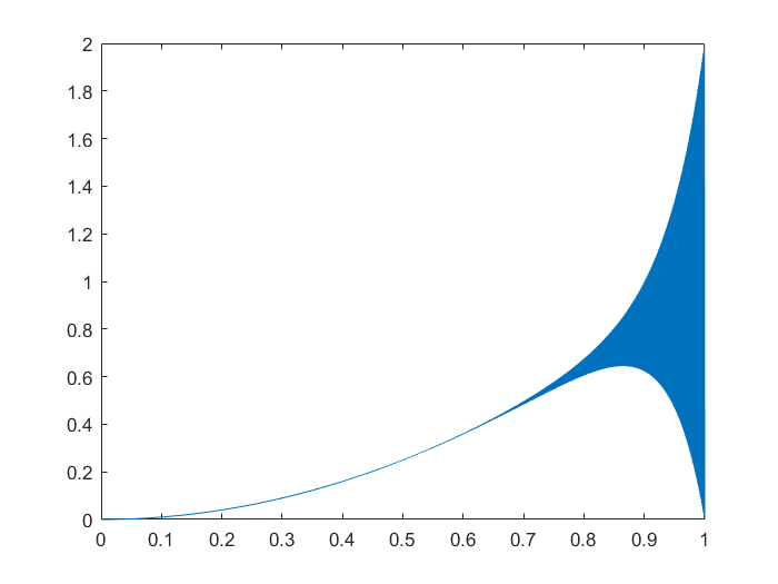
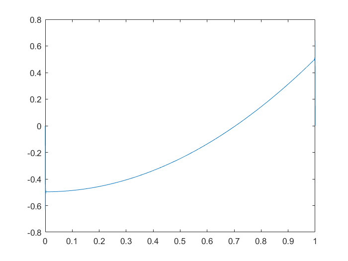
Figure 6.1. $\varepsilon=10^{-6}$. Left: Linear, Right: SPLS

6.2. Streamline Diffussion versus PG discretization

For the second test, we take $f=2x$ and compare Streamline Diffusion and Petrov-Galerkin. In this case, the exact solution will have a boundary layer at $x=1$ of width $|\varepsilon\log(\varepsilon)|$. We include two tables for this test where the error is measured only on a subdomain of $[0,1]$ excluding 1% of the nodes near the right boundary. Table 3 compares the errors of the SD approximation $u_{h,sd}$ with the PG approximation $u_{h,pg}$ in the SD norm $||u-u_{h}||_{sd}$. As we can see in Table 3, the expected order for SD is observed. Further, the same order is attained by PG, with errors of smaller magnitude.

Level/$\varepsilon$	$10^{-4}$
	$||u-u_{h,sd}||_{sd}$	Order	$||u-u_{h,pg}||_{sd}$	Order
1	1.56e-02	-	1.54e-02	-
2	2.57e-03	2.60	2.51e-03	2.62
3	5.45e-04	2.24	4.92e-04	2.35
4	1.05e-04	2.37	4.21e-05	3.55
5	3.86e-05	1.45	1.54e-05	1.46
6	1.45e-05	1.41	5.78e-06	1.41
Level/$\varepsilon$	$10^{-8}$
	$||u-u_{h,sd}||_{sd}$	Order	$||u-u_{h,pg}||_{sd}$	Order
1	1.46e-02	-	1.45e-02	-
2	2.16e-03	2.76	2.09e-03	2.79
3	3.98e-04	2.44	3.16e-04	2.72
4	1.01e-04	1.97	4.04e-05	2.97
5	3.60e-05	1.50	1.43e-05	1.50
6	1.27e-05	1.50	5.06e-06	1.50

Table 3. SD vs. PG: $f(x)=2x$

In Table 3 and Table 4, the SD and PG approximations are compared in the optimal norm $||u-u_{h}||_{*,h}$ for $f(x)=2x$. The results are interesting as not only does the PG approximation have significantly smaller errors, but also it attains higher order of approximation. In this case ($\varepsilon<h$), in accordance with Theorem 5.6, $\mathcal{O}(h^{2})$ is obtained for the PG method. For the streamline diffusion approximation, the optimal norm only appears to achieve order one, see Table 4.

Level/$\varepsilon$	$10^{-4}$
	$||u-u_{h,sd}||_{*,h}$	Order	$||u-u_{h,pg}||_{*,h}$	Order
1	5.47e-03	0.00	2.32e-03	0.00
2	2.75e-03	0.99	2.68e-04	3.11
3	1.42e-03	0.95	3.71e-05	2.85
4	7.19e-04	0.99	1.61e-06	4.53
5	3.62e-04	0.99	4.27e-07	1.92
6	1.82e-04	0.99	1.21e-07	1.82
Level/$\varepsilon$	$10^{-8}$
	$||u-u_{h,sd}||_{*,h}$	Order	$||u-u_{h,pg}||_{*,h}$	Order
1	5.43e-03	0.00	2.17e-03	0.00
2	2.76e-03	0.98	2.21e-04	3.30
3	1.43e-03	0.95	2.30e-05	3.26
4	7.20e-04	0.99	1.48e-06	3.95
5	3.62e-04	0.99	3.71e-07	2.00
6	1.82e-04	0.99	9.29e-08	2.00

Table 4. SD vs. PG:$f(x)=2x$

Level/$\varepsilon$	$10^{-4}$
	$\|u-u_{h,sd}\|_{B}$	Order	$\|u-u_{h,pg}\|_{B}$	Order
1	1.12e-02	-	2.33e-03	0.00
2	5.74e-03	0.96	2.69e-04	3.12
3	2.92e-03	0.97	3.71e-05	2.85
4	1.47e-03	0.99	1.73e-06	4.43
5	7.38e-04	0.99	4.55e-07	1.92
6	3.70e-04	1.00	1.27e-07	1.84
Level/$\varepsilon$	$10^{-8}$
	$\|u-u_{h,sd}\|_{B}$	Order	$\|u-u_{h,pg}\|_{B}$	Order
1	1.12e-02	-	2.18e-03	0.00
2	5.74e-03	0.96	2.21e-04	3.30
3	2.93e-03	0.97	2.30e-05	3.26
4	1.47e-03	0.99	1.61e-06	3.83
5	7.38e-04	0.99	4.04e-07	2.00
6	3.70e-04	1.00	1.01e-07	2.00

Table 5. SD vs. PG:$f(x)=2x$

As reflected by the numerical result presented in Table 5, the computations using a mixed balanced norm

$$\|u\|_{B}^{2}=(\epsilon+\delta)^{2}|u|^{2}+\|u\|^{2},$$

where $\delta=\frac{2h}{3}$ is parameter from the optimal norm, show $\mathcal{O}(h)$ order of approximation for the Streamline Difussion method, and $\mathcal{O}(h^{2})$ for the upwinding Petrov Galerkin method.

7. Conclusion

We analyzed and compared four discretization methods for a model
convection-diffusion problem. A unified error analysis was possible because of our representation of the optimal norm on the trial spaces. The ideas presented in this paper are stepping stones for introducing and analyzing new and efficient discretizations for the multi-dimensional cases of convection dominated problems.

Our finite element analysis for the considered model problem showed that the best method is the upwinding PG method. When compared with the standard SUPG method, we observed that the upwinding PG method can provide higher order of approximation in particular norms. In addition, we proved that, due to reformulation as a mixed conforming method, the upwinding PG method leads to stability and good approximability results under less regularity assumptions for the solution.

For the $(P^{1}-P^{2})$-SPLS method, we proved that the seminorm part of the optimal trial norm becomes a norm which makes the error analysis much simpler.

Results on generalizing the upwinding PG and SPLS discretizations for singularly perturbed problems on two or more dimensions are to be discussed in a separate publication.

References

• [1] A. Aziz and I. Babuška. Survey lectures on mathematical foundations of the finite element method. The Mathematical Foundations of the Finite Element Method with Applications to Partial Differential Equations, A. Aziz, editor, 1972.
• [2] C. Bacuta. Schur complements on Hilbert spaces and saddle point systems. J. Comput. Appl. Math., 225(2):581–593, 2009.
• [3] C. Bacuta, D. Hayes, and J. Jacavage. Notes on a saddle point reformulation of mixed variational problems. Comput. Math. Appl., 95:4–18, 2021.
• [4] C. Bacuta, D. Hayes, and J. Jacavage. Efficient discretization and preconditioning of the singularly perturbed reaction-diffusion problem. Comput. Math. Appl., 109:270–279, 2022.
• [5] C. Bacuta and J. Jacavage. A non-conforming saddle point least squares approach for an elliptic interface problem. Comput. Methods Appl. Math., 19(3):399–414, 2019.
• [6] C. Bacuta and J. Jacavage. Saddle point least squares preconditioning of mixed methods. Computers & Mathematics with Applications, 77(5):1396–1407, 2019.
• [7] C. Bacuta and J. Jacavage. Least squares preconditioning for mixed methods with nonconforming trial spaces. Applicable Analysis, Available online Feb 27, 2019:1–20, 2020.
• [8] C. Bacuta and P. Monk. Multilevel discretization of symmetric saddle point systems without the discrete LBB condition. Appl. Numer. Math., 62(6):667–681, 2012.
• [9] C. Bacuta and K. Qirko. A saddle point least squares approach to mixed methods. Comput. Math. Appl., 70(12):2920–2932, 2015.
• [10] C. Bacuta and K. Qirko. A saddle point least squares approach for primal mixed formulations of second order PDEs. Comput. Math. Appl., 73(2):173–186, 2017.
• [11] Cr. Bacuta and C. Bacuta. Connections between finite difference and finite element approximations. Appl. Anal., 102(6):1808–1820, 2023.
• [12] S. Bartels. Numerical approximation of partial differential equations, volume 64 of Texts in Applied Mathematics. Springer, [Cham], 2016.
• [13] D. Boffi, F. Brezzi, L. Demkowicz, R. G. Durán, R. Falk, and M. Fortin. Mixed finite elements, compatibility conditions, and applications, volume 1939 of Lecture Notes in Mathematics. Springer-Verlag, Berlin; Fondazione C.I.M.E., Florence, 2008. Lectures given at the C.I.M.E. Summer School held in Cetraro, June 26–July 1, 2006, Edited by Boffi and Lucia Gastaldi.
• [14] D. Boffi, F. Brezzi, and M. Fortin. Mixed finite element methods and applications, volume 44 of Springer Series in Computational Mathematics. Springer, Heidelberg, 2013.
• [15] T. Bouma, J. Gopalakrishnan, and A. Harb. Convergence rates of the DPG method with reduced test space degree. Comput. Math. Appl., 68(11):1550–1561, 2014.
• [16] F. Brezzi, D. Marini, and A. Russo. Applications of the pseudo residual-free bubbles to the stabilization of convection-diffusion problems. Comput. Methods Appl. Mech. Engrg., 166(1-2):51–63, 1998.
• [17] D. Broersen and R. Stevenson. A robust Petrov-Galerkin discretisation of convection-diffusion equations. Comput. Math. Appl., 68(11):1605–1618, 2014.
• [18] L. Demkowicz C. Carstensen and J. Gopalakrishnan. Breaking spaces and form for the DPG method and applications including maxwell equations. Computers and Mathematics with Applications, 72:494–522, 2016.
• [19] J. Chan, N. Heuer, T. Bui-Thanh, and L. Demkowicz. A robust DPG method for convection-dominated diffusion problems II: adjoint boundary conditions and mesh-dependent test norms. Comput. Math. Appl., 67(4):771–795, 2014.
• [20] L. Chen and J. Xu. Stability and accuracy of adapted finite element methods for singularly perturbed problems. Numer. Math., 109(2):167–191, 2008.
• [21] A. Cohen, W. Dahmen, and G. Welper. Adaptivity and variational stabilization for convection-diffusion equations. ESAIM Math. Model. Numer. Anal., 46(5):1247–1273, 2012.
• [22] L. Demkowicz, T. Führer, N. Heuer, and X. Tian. The double adaptivity paradigm (how to circumvent the discrete inf-sup conditions of Babuška and Brezzi). Technical report, 2021.
• [23] L. Demkowicz and J. Gopalakrishnan. A class of discontinuous Petrov-Galerkin methods. Part I: the transport equation. Comput. Methods Appl. Mech. Engrg., 199(23-24):1558–1572, 2010.
• [24] L. Demkowicz and J. Gopalakrishnan. A class of discontinuous Petrov–Galerkin methods. ii. optimal test functions. Numerical Methods for Partial Differential Equations, 27(1):70–105, 2011.
• [25] L. Demkowicz and L. Vardapetyan. Modelling electromagnetic/scattering problems using hp-adaptive finite element methods. Comput, Methods Appl. Mech. Engrg. Numerical Mathematics, 152:103 – 124, 1998.
• [26] J. Gopalakrishnan. Five lectures on DPG methods. arXiv 1306.0557, 2013.
• [27] T. J. R. Hughes and A. Brooks. A multidimensional upwind scheme with no crosswind diffusion. In Finite element methods for convection dominated flows (Papers, Winter Ann. Meeting Amer. Soc. Mech. Engrs., New York, 1979), volume 34 of AMD, pages 19–35. Amer. Soc. Mech. Engrs. (ASME), New York, 1979.
• [28] K. W. Morton J. W. Barrett, and. Optimal Petrov-Galerkin methods through approximate symmetrization. IMA J. Numer. Anal., 1(4):439–468, 1981.
• [29] T. Kato. Estimation of iterated matrices, with application to the Von Neumann condition. Numer. Math., 2:22–29, 1960.
• [30] R. Lin and M. Stynes. A balanced finite element method for singularly perturbed reaction-diffusion problems. SIAM Journal on Numerical Analysis, 50(5):2729–2743, 2012.
• [31] T. Linß. Layer-adapted meshes for reaction-convection-diffusion problems, volume 1985 of Lecture Notes in Mathematics. Springer-Verlag, Berlin, 2010.
• [32] Alfio Quarteroni, Riccardo Sacco, and Fausto Saleri. Numerical mathematics, volume 37 of Texts in Applied Mathematics. Springer-Verlag, Berlin, second edition, 2007.
• [33] H.-G. Roos, M. Stynes, and L. Tobiska. Numerical methods for singularly perturbed differential equations, volume 24 of Springer Series in Computational Mathematics. Springer-Verlag, Berlin, 1996. Convection-diffusion and flow problems.
• [34] H.G. Roos and M. Schopf. Convergence and stability in balanced norms of finite element methods on shishkin meshes for reaction-diffusion problems: Convergence and stability in balanced norms. ZAMM Journal of applied mathematics and mechanics: Zeitschrift für angewandte Mathematik und Mechanik, 95(6):551–565, 2014.
• [35] J. Xu and L. Zikatanov. Some observations on Babuška and Brezzi theories. Numer. Math., 94(1):195–202, 2003.