AONeuS: A Neural Rendering Framework for Acoustic-Optical Sensor Fusion

Abstract

Underwater perception and 3D surface reconstruction are challenging problems with broad applications in construction, security, marine archaeology, and environmental monitoring. Treacherous operating conditions, fragile surroundings, and limited navigation control often dictate that submersibles restrict their range of motion and, thus, the baseline over which they can capture measurements. In the context of 3D scene reconstruction, it is well-known that smaller baselines make reconstruction more challenging. Our work develops a physics-based multimodal acoustic-optical neural surface reconstruction framework (AONeuS) capable of effectively integrating high-resolution RGB measurements with low-resolution depth-resolved imaging sonar measurements. By fusing these complementary modalities, our framework can reconstruct accurate high-resolution 3D surfaces from measurements captured over heavily-restricted baselines. Through extensive simulations and in-lab experiments, we demonstrate that AONeuS dramatically outperforms recent RGB-only and sonar-only inverse-differentiable-rendering–based surface reconstruction methods.

1 Introduction

The 3D reconstruction of underwater environments is an important problem with applications in myriad fields, including underwater construction, marine ecology, archaeology, mapping, inspection, and surveillance [1, 25, 45, 33]. The underwater robots applied to this task are typically equipped with both imaging sonars (i.e., acoustic cameras) and optical cameras [23, 28]. These sensors capture complementary information about their operating environments.

Forward-look imaging sonars consist of a uniform linear array of transducers which, through beamforming, recover both range and azimuth information (but not elevation). (3D imaging sonars which record both azimuth and elevation also exist, but can be prohibitively expensive.) Unlike light-based sensors, imaging sonars are highly robust to scattering and low-light conditions. Unfortunately, imaging sonars generally have poor spatial resolution; sonar images of an object of interest often appear textureless and hard to recognize; and imaging sonar measurements can suffer from complex artifacts caused by multipath reflections and the variable speed of sound passing through inhomogeneous water [44].

By contrast, optical cameras have high spatial resolution and can resolve object appearance in great detail. However, in turbid water light scattering and absorption can severely restrict the range and contrast of optical cameras [18]. Moreover, to recover depth information passive optical sensors rely on large displacements/baselines between measurements. In constrained operating environments, such measurements are often inaccessible.

By leveraging the complementary strengths and weaknesses of cameras and imaging sonars, acoustic-optical sensor fusion promises to enable robust and high-resolution underwater perception and scene reconstruction [16, 31]. Existing contour matching based acoustic-optical reconstruction methods based can already reconstruct accurate high-resolution 3D surfaces [8]. Unfortunately, these methods require a 360-degree view of the scene and are inapplicable in the small-baseline operating conditions prevalent in real-world unmanned underwater vehicle operation. Alternatively, one can reconstruct the scene from optical and acoustic measurements independently and then fuse the result [20]. However, this simple approach provides limited benefits over camera-only surface reconstruction.

In this paper, we develop an inverse-differentiable-rendering–based approach to acoustic-optical sensor fusion that can form dense 3D surface reconstructions from camera and sonar measurements captured across a small baseline. Our work consists of four key contributions.

• We develop a physics-based multimodal acoustic-optical neural surface framework which simultaneously integrates RGB and imaging sonar measurements. Our approach extends the neural surfaces 3D reconstruction framework [46] by combining a unified representation of the scene geometry with modality-specific (acoustic and optical) representations of appearance.

• We conduct experiments on both synthetic and experimentally-captured datasets and demonstrate our method can effectively reconstruct high-fidelity surface geometry from noisy measurements captured over limited baselines.

• We theoretically support our strong empirical performance by analyzing the conditioning of the acoustic-optical forward model. We show that the forward process associated with triangulating a point in 3D from acoustic-optical measurements is better conditioned and easier to invert the unimodal forward models.

• We release a public dataset and open-source implementation of our method.

2 Related Work

Sonar Imaging

3D reconstruction from sonar imagery is an important and widely studied problem. Over the last decade a variety of 3D reconstruction methods have been proposed based on space carving [5, 6], classical point-cloud processing algorithms [43, 51], generative modeling [5, 7, 35, 50], convex optimization [52], graph-based processing [47, 48], and supervised machine learning [15, 49, 3].

Last year, two research groups employed neural rendering to enable breakthrough 3D sonar imaging performance. Qadri et al. [39] developed a Neural Implicit Surface Reconstruction Using Imaging Sonar (NeuSIS) method which forms high-fidelity 3D surface reconstructions from forward imaging sonar measurements by combining neural surface representations with a novel acoustic differentiable volumetric renderer. Similarly, Reed et al. [40] employed neural rendering to recover 3D volumes from synthetic aperture sonar measurements. The former method relies upon a large number of sonar images captured over a large baseline while the latter applies to synthetic aperture sonar, not forward imaging sonar, and relies on access to raw time-based sonar measurements. These methods represent the state-of-the-art in 3D surface reconstruction with sonar.

To date, no method has effectively recovered a dense 3D scene from 2D sonar images captured over a limited baseline. Without additional constrains, e.g., optical measurements, or strong priors the reconstruction problem is hopelessly underdetermined.

Neural Rendering

In their breakthrough neural radiance fields (NeRF) paper, Mildenhall et al. [32] combined neural signal representations with differentiable volume rendering to perform novel view synthesis. The underlying differentiable volume rendering concept has since been extended to represent and recover scene geometry. The Implicit Differentiable Renderer (IDR) approach, introduced in  [53], represents geometry as the zero-level set of a neural network and uses differentiable surface rendering to fit the parameters of a neural network. IDR requires object masks for supervision. Later methods, like Neural Surfaces (NeuS) [46], Unified Surfaces (UNISURF) [37], and Volume Signed Distance Functions (VolSDF) [54] combine an implicit surface representation with differentiable volume rendering to recover 3D geometry from images without the need for object masks. Recent work has sought to reduce the number of training images required [29] and to accelerate rendering to enable real-time applications [55].

The inverse-differentiable-rendering framework has also been extended to handle measurements from a diverse range of sensors. Cross-spectral radiance fields (X-NeRF) were proposed in [38] to model multispectral, infrared, and RGB images. Transient neural radiance fields were proposed in [30] to model the measurements from a single-photon lidar. Time-of-flight radiance fields were proposed in  [4] to model the measurements from a continuous wave time-of-flight sensor. Polarization-aided decomposition of radiance, or PANDORA, was proposed in [14] to model polarimetric measurements of light. Radar neural radiance fields (RaNeRF) were proposed in [27] to model inverse synthetic aperture radar measurements.

Several recent works have modeled light scattering within the neural rendering framework to improve reconstructions through water [42, 24], haze [12], and fog [2].

Multimodal Imaging

To overcome the disadvantages inherent to using a single sensing modality, numerous multimodal sensing algorithms have been developed [22, 26, 36, 10]. Most related to our work, Babaee and Negahdaripour [8] reconstruct 3D objects from RGB and sonar imagery by matching occluding contours across RGB images and imaging sonar measurements, performing stereo matching, and interpolating the curves in 3D space. Unfortunately, this method is inapplicable to the small-baseline setting; it fundamentally requires 360-degree views of the scene. Another work that reconstructions 3D from RGB images and imaging sonar is [20]. This work reconstructs a scene from optical and acoustic measurements independently using classical methods like COLMAP [41] and then fuses the result. As we will demonstrate in Sec. 6.2, this approach provides limited benefits over a purely optical approach and is not competitive with sate-of-the-art neural rendering based methods.

Outside of sonar, several neural-rendering based approaches to sensor fusion have recently been developed. In Multimodal Neural Radiance Field, Zhu et al. [56] use neural rendering to combine RGB, thermal, and point cloud data. Similarly, [21] use neural rendering to combine multispectral measurements of different polarizations and Carlson et al. [11] fuse sparse lidar and RGB measurements to build 3D occupancy grid of unbounded scenes,

To our knowledge, ours is the first work to perform acoustic-optical sensor fusion with neural rendering.

3 Background

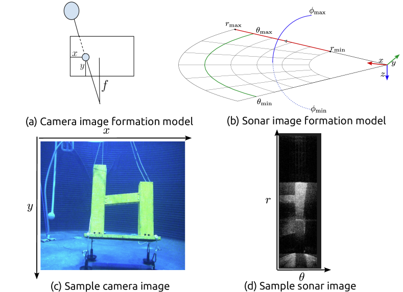
Figure 2: Acoustic-Optical Measurement Processes. (a) RGB measurement process and example measurement. Pixels along a common ray passing through the camera center map to the same image pixel on the image plane. (b) Sonar measurement process and example measurement. In a sonar image, the azimuth $\theta$ and range $r$ of the imaged object are resolved. However, the elevation information $\phi$ is lost; all objects located along the elevation arc in blue map to the same pixel.

3.1 Imaging Sonars

Imaging sonars are active sensors that emit acoustic pulses and measure the intensity of the reflected wave. They produce a 2D acoustic image in which the range and azimuth of the imaged object are resolved. However, the object’s elevation remains ambiguous. I.e., the reflecting object can be located anywhere on the elevation arc (fig. 2) and the intensity of a pixel in a sonar image is proportional to the cumulative reflected acoustic energy from all reflecting points along the elevation arc.

3.2 Image Formation Model of an Imaging Sonar

Similar to [39], we use the following sonar image formation model:

$$\!\!\!\!I^{\text{son}}(r_{i},\theta_{i})\!=\!\!\int_{\phi_{\text{min}}}^{\phi_{\text{max}}}\!\int_{r_{i}-\epsilon}^{r_{i}+\epsilon}\frac{\textit{E}_{e}}{r}T(r,\theta_{i},\phi)\sigma(r,\theta_{i},\phi)\text{d}r\text{d}\phi,$$ (1)

where $\phi_{\text{min}},\phi_{\text{max}}$ are the minimum and maximum elevation angles, $E_{e}$ is the acoustic energy emitted by the sonar. $T=e^{-\int_{0}^{r_{i}}\sigma(r^{\prime},\theta_{i},\phi_{i})\text{d}r^{\prime}}$ is the transmittance term, and $\sigma$ is the particle density. (See [39] for more details.)

3.3 Image Formation Model of an Optical Camera

We adopt the optical camera image formation model proposed by [46] where a pixel intensity at $(x,y)$ is approximated by:

$$I^{\text{cam}}(x,y)=\int_{0}^{\infty}T(t)\sigma(t)c(\mathbf{p}(t),\mathbf{v})dt,$$ (2)

where the integral is over the ray starting at the camera center and passing through pixel $(x,y)$. $T,\sigma$ are the transmittance and density values at point $p(t)$, and $c(\mathbf{p}(t),\mathbf{v})$ is the color of a point viewed from direction $\mathbf{v}$.

4 Problem Statement

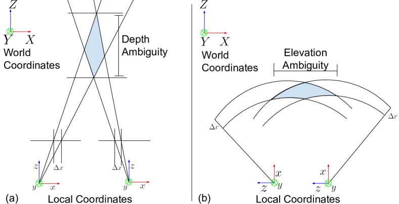
Figure 3: Acoustic-Optical Measurement Ambiguities. (a) Two RGB measurements captured over a limited baseline struggle to localize a point along the depth-axis. (b) Two sonar measurements captured over a limited baseline struggle to localize a point along the x-axis. Because they have orthogonal ambiguities, RGB and sonar measurements are highly complementary.

Our goal in this work is to reconstruct the 3D surface of an underwater object using a small collection of RGB and sonar measurements captured over a limited baseline. Specifically, we assume access to two datasets, $\mathcal{D}^{\text{cam}}=\{I_{i}^{\text{cam}},P_{i}^{\text{son}}\}$ and $\mathcal{D}^{\text{son}}=\{I_{i}^{\text{son}},P_{i}^{son}\}$, consisting of RGB/sonar images and their respective poses.

Given a large dataset captured over a sufficiently diverse range of poses (e.g., thousands of images captured from 360-degrees [39]), existing unimodal (camera-only/sonar-only) surface reconstruction methods are already effective [39, 46]. In this work, we focus on the small baseline operating conditions—pervasive in underwater robotics—where optical cameras record insufficient information to recover depth information (see Fig. 3(a)) and imaging sonars record insufficient information to recover elevation information (see Fig. 3(b)).

Specifically, we introduce a physics-based multimodal inverse-differentiable-rendering framework that integrates information from both acoustic and optical sensors to generate accurate 3D reconstructions. Our approach automatically exploits the complementary information (elevation/range) provided by each sensor.

Because our shared pool-based testing facility does not allow us to introduce turbidity, in this work we focus on the clear-water setting. Modeling the effects of light scattering in our forward model [42, 24, 2, 12] would likely improve our system’s in-the-wild performance.

5 Method

5.1 Acoustic-Optical NeuS

Our AONeuS reconstruction framework is illustrated in Fig. 4. Following Wang et al. [46], Qadri et al. [39], we represent the object’s surface using a Signed Distance Function (SDF), $\mathbf{N}(\mathbf{x})$, which outputs the distance of each 3D point $\mathbf{x}=(\mathbf{X},\mathbf{Y},\mathbf{Z})$ to the nearest surface. Distinct from these works, we use two separate rendering neural networks ($\textbf{M}^{\text{cam}}$ and $\textbf{M}^{\text{son}}$) that approximate the optical and acoustic outgoing radiance at each spatial coordinate $\mathbf{x}$. This choice is motivated by the fact that different materials have different acoustic and optical reflectance properties. For example, glass is invisible to optical cameras but visible to imaging sonar, and PVC is invisible to imaging sonar but visible to optical cameras.

In this work, we sample and sum points along acoustic and optical rays to approximate the rendering integrals defined by Eq. 1 and Eq. 2. Our rendering functions can be expressed as

$$\hat{I}^{\text{son}}(r,\theta)=\sum_{\mathbf{x}\in\mathcal{A}_{p^{\text{son}}}}\frac{1}{r(\mathbf{x})}T[\mathbf{x}]\alpha[\mathbf{x}]\mathbf{M}^{\text{son}}(\mathbf{x}),\text{ and }$$ (3)

$$\hat{I}^{\text{cam}}(x,y)=\sum_{\mathbf{x}\in\mathcal{R}_{p^{\text{cam}}}}T[\mathbf{x}]\alpha[\mathbf{x}]\mathbf{M}^{\text{cam}}(\mathbf{x}),$$ (4)

where $\mathcal{A}_{p^{\text{son}}}$ is the set sampled points along the acoustic arc at pixel $p^{\text{son}}$ and $\mathcal{R}_{p^{\text{cam}}}$ is the set of sampled points along optical ray passing through pixel $p^{\text{cam}}$. $\mathbf{M}^{\text{son}}$ and $\mathbf{M}^{\text{cam}}$ are the predicted radiance at $\mathbf{x}$.

The computation of the discrete transmittance and opacity terms in Eq. 3 and Eq. 4 requires sampling along both acoustic and optical rays. For any such spatial sample $\mathbf{x}_{s}$, (i.e., any point along an acoustic or optical ray), the discrete opacity at $\mathbf{x}_{s}$ can be approximated as

$$\alpha[\mathbf{x}_{s}]=\max\left(\frac{\mathbf{\Phi}_{s}(\mathbf{N}(\mathbf{x}_{s}))-\mathbf{\Phi}_{s}(\mathbf{N}(\mathbf{x}_{s+1}))}{\mathbf{\Phi}_{s}(\mathbf{N}(\mathbf{x}_{s}))},0\right),$$ (5)

where $\mathbf{\Phi}_{s}(x)=(1+e^{-sx})^{-1}$ is the Sigmoid function and $s$ is a trainable parameter. The discrete transmittance is modeled as

$$T[\mathbf{x_{s}}]=\prod_{\mathbf{x_{r}}\;|\;r<s}(1-\alpha[\mathbf{x_{r}}]).$$ (6)

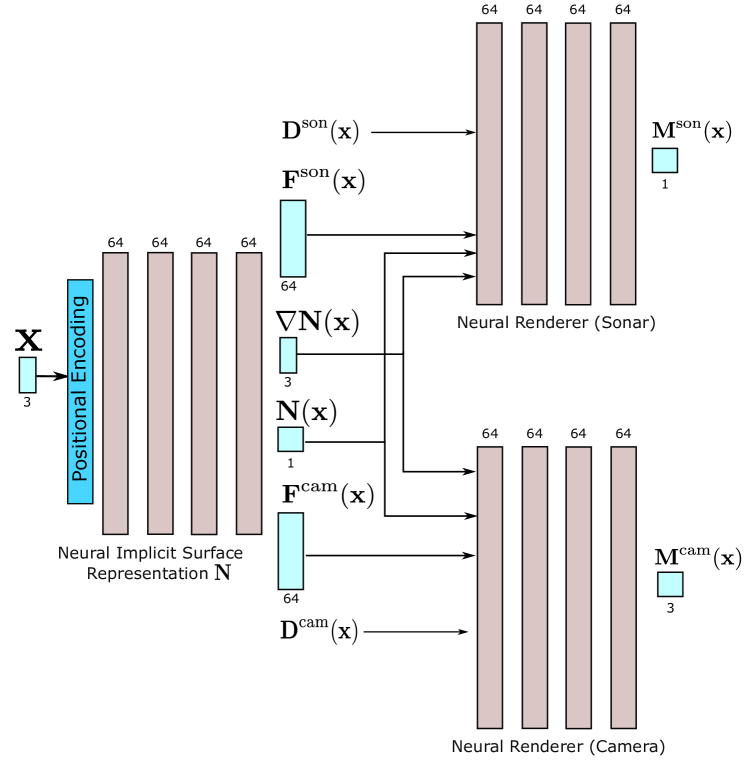
Figure 4: AONeuS Reconstruction Framework. A shared surface geometry SDF network $\mathbf{N}$ is used in combination with rendering specific neural rendering modules. For each sampled point $\mathbf{x}$ along an acoustic or optical ray, $\mathbf{N}$ outputs its signed distance, its gradient as well as 2 features vectors $\mathbf{F}^{\text{son}}$ and $\mathbf{F}^{\text{cam}}$ all serving as input to their respective rendering networks.

5.1.1 Loss Function

Our loss function comprises the sonar and camera intensity losses:

$$\mathcal{L}_{\text{int}}^{\text{son}}\equiv\frac{1}{\mathbf{N}_{\mathcal{P^{\text{son}}}}}\sum_{p\in\mathcal{P}^{\text{son}}}||\hat{I}(p)-I(p)||_{1},\text{ and }$$ (7)

$$\mathcal{L}_{\text{int}}^{\text{cam}}\equiv\frac{1}{\mathbf{N}_{\mathcal{P^{\text{cam}}}}}\sum_{p\in\mathcal{P}^{\text{cam}}}||\hat{I}(p)-I(p)||_{1},$$ (8)

where $\mathcal{P}^{\text{cam}}$ and $\mathcal{P}^{\text{son}}$ is the set of sampled pixels in the camera and sonar images respectively. We additionally use the eikonal loss as an implicit regularization to encourage smooth reconstructions:

$$\mathcal{L}_{\text{eik}}\equiv\frac{1}{|\mathbf{X}|}\sum_{\mathbf{x}\in\mathbf{X}}(||\nabla\mathbf{N}(\mathbf{x})||_{2}-1)^{2},$$ (9)

where $\mathbf{X}$ is the set of all sampled points.

We also utilize an $\ell_{1}$ loss term as an additional prior term which biases the network towards reconstructions that minimize the total opacity of the scene (for example in cases where the object is on the seafloor and only specific sides can be imaged):

$$\mathcal{L}_{\text{reg}}\equiv\frac{1}{|\mathbf{X}|}\sum_{\mathbf{x}\in\mathbf{X}}||\alpha[\mathbf{x}]||_{1}.$$ (10)

Hence, our total loss is

$$\mathcal{L}=\alpha(t)\mathcal{L}_{\text{int}}^{\text{son}}+(1-\alpha(t))\mathcal{L}_{\text{int}}^{\text{cam}}+\lambda_{\text{eik}}\mathcal{L}_{\text{eik}}+\lambda_{\text{reg}}\mathcal{L}_{\text{reg}}.$$ (11)

The network is trained with the ADAM optimizer.

5.1.2 Weight Scheduling

The weights assigned to the sonar and camera intensity losses (respectively $\alpha(t)$ and $1-\alpha(t)$ in eq. 11) impact the reconstruction quality as they determine which measurements the network should emphasize throughout training. We adopt a simple two-step weighting scheme:

$$\alpha(t)=\begin{cases}1\text{ if }t<E_{t},\\ \lambda\text{ if }E_{t}<t<E_{e}.\end{cases}$$ (12)

In the early iterations, $t<E_{t}$, the sonar measurements are used exclusively and serve to ”mask“ the object; i.e., update the weights of the SDF network $\mathbf{N}$ to bias it towards reconstructions in which the geometry of the object are better constrained in the depth direction. This process establishes an initialization for the later iterations.

In later iterations, $t>E_{t}$, more emphasis is placed on the camera measurements. These measurements cosntrain the $x$ and $y$ directions and help resolve the elevation ambiguity inherent in sonar data. In this phase, sonar measurements receive less weight and act as a depth regularizer.

6 Experimental Results

In this section we evaluate the proposed AONeuS technique on both synthetic and experimentally captured data.

6.1 Results on Synthetic Data

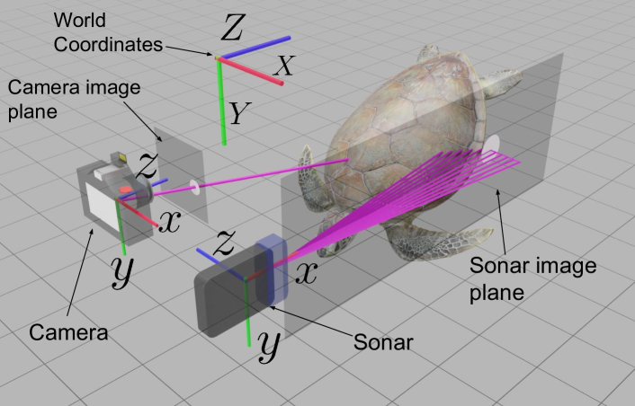
Figure 5: Simulation setup. We simulate capturing sonar and camera measurements over a limited baseline.

To generate synthetic measurements, we implemented the sonar image formation model Eq. 1 in Blender [13] and collected simulated sonar-camera datasets for various objects. The simulation setup is illustrated in Fig. 5. The sonar and camera are approximately collocated, and are translated linearly over a short baseline along the $X$ axis of the world frame for a distance of 1.2 with the sonar’s azimuthal plane parallel the YZ plane in the world frame. The sonar’s azimuthal plane is oriented orthogonal to the direction of motion to ensure the trajectory was non-degenerate; multiple measurements captured from positions within the azimuthal plane of the sonar would be highly redundant and uninformative [33].

For each object, the trajectory is sub-sampled into smaller baselines: 0.96, 0.72, 0.48, and 0.24 for analysis. We scaled the meshes so that the objects are approximately $\sim 1m$ in size and the sensors are placed about 1.5–2 away from the object. The elevation aperture of the sonar is $12^{\circ}$. We benchmark our method against two methods: NeuS [46] and NeuSIS [39], executing all methods 9 times with randomly initialized seeds. To ensure we had reasonable camera-only results, we provided NeuS with masks of the object. This information is not required by nor provided to NeuSIS and AONeuS.

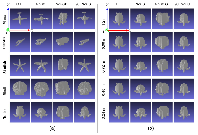
Figure 9: Simulated Reconstructions Over Varying Baselines. ((5x5 collection of images) 1st column: Ground truth mesh and measurement geometry. 2nd column: Sonar-only neural surface reconstructions. 3rd row: RGB-only neural surface reconstructions. 4th column: Multimodal backprojection reconstruction. 5th column: Multimodal neural surface reconstructions. (The rows show 1m, 80cm, 60cm, 40cm, and 20cm baseline reconstructions, respectively (or something like that).) (This is transposed from what we discussed yesterday and includes multimodal back-prop).) .

In Fig. 9(a), we compare the reconstruction performance of all three techniques for a total of five scenes. We could observe that AONeus consistently reconstructs the scene geometry better than NeuS and NeuSIS. Further, we can also observe that NeuS (camera-only) incorrectly reconstructs the depth axis ($Z$-axis) whereas NeuSIS (sonar-only) can reconstruct only the depth-axis accurately. The proposed AONeus was able to recover underlying scene geometry along all the axes.

		NeuS	NeuSIS	AONeuS
1.2m	Chamfer $\boldsymbol{\downarrow}$	$0.123\pm 0.028$	$0.130\pm 0.013$	$\mathbf{0.075}\pm 0.006$
	Precision$\boldsymbol{\uparrow}$	$0.653\pm 0.095$	$0.566\pm 0.043$	$\mathbf{0.862}\pm 0.042$
	Recall $\boldsymbol{\uparrow}$	$0.526\pm 0.134$	$\mathbf{0.836}\pm 0.022$	$0.825\pm 0.056$
0.96m	Chamfer $\boldsymbol{\downarrow}$	$0.139\pm 0.024$	$0.134\pm 0.011$	$\mathbf{0.079}\pm 0.005$
	Precision $\boldsymbol{\uparrow}$	$0.602\pm 0.076$	$0.531\pm 0.031$	$\mathbf{0.840}\pm 0.017$
	Recall $\boldsymbol{\uparrow}$	$0.470\pm 0.132$	$\mathbf{0.816}\pm 0.031$	$0.807\pm 0.017$
0.72m	Chamfer $\boldsymbol{\downarrow}$	$0.205\pm 0.027$	$0.135\pm 0.011$	$\mathbf{0.081}\pm 0.005$
	Precision $\boldsymbol{\uparrow}$	$0.423\pm 0.051$	$0.537\pm 0.062$	$\mathbf{0.810}\pm 0.032$
	Recall $\boldsymbol{\uparrow}$	$0.279\pm 0.071$	$0.768\pm 0.029$	$\mathbf{0.792}\pm 0.022$
0.48m	Chamfer $\boldsymbol{\downarrow}$	$0.249\pm 0.045$	$0.139\pm 0.012$	$\mathbf{0.088}\pm 0.006$
	Precision $\boldsymbol{\uparrow}$	$0.337\pm 0.062$	$0.470\pm 0.028$	$\mathbf{0.791}\pm 0.023$
	Recall $\boldsymbol{\uparrow}$	$0.189\pm 0.074$	$0.706\pm 0.028$	$\mathbf{0.770}\pm 0.023$
0.24m	Chamfer $\boldsymbol{\downarrow}$	$0.406\pm 0.087$	$0.146\pm 0.009$	$\mathbf{0.111}\pm 0.017$
	Precision $\boldsymbol{\uparrow}$	$0.223\pm 0.060$	$0.450\pm 0.028$	$\mathbf{0.690}\pm 0.045$
	Recall $\boldsymbol{\uparrow}$	$0.107\pm 0.049$	$0.587\pm 0.042$	$\mathbf{0.679}\pm 0.042$

Table 1: Metrics for synthetic turtle data. Best metrics are bolded.

In Fig. 9(b), we show the results for the turtle mesh for various baselines. To visualize the ambiguities associated with camera and sonar modalities and the benefit of the fusion algorithm, we rendered the reconstructed meshes with a virtual camera pointing in $Y$-axis. Hence, the rendered images are projections of the reconstructed mesh on $ZX$-plane. As we decrease the baseline (top to bottom), for NeuS, we observe an increasing loss of features along depth direction: the back legs of the turtle are progressively lost and depth-reconstruction worsens with decreasing baselines. For sonar-only methods, significant ambiguities along the elevation axis can be seen across all baselines: due to the limited translation of the sonar, the collected measurements are not enough to constrain and resolve the turtle shell adequately. Our framework AONeuS integrates orthogonal information from both imaging modalities to yield reconstructions of higher quality across all baselines: all features of the turtle including its shell and its back legs are clearly discernible. These observations are further supported by the quantitative analysis in Tab. 1 where we report the mean and variance of Chamfer $L_{1}$ distance, precision, and recall of the reconstructions over nine trials. The results demonstrate that AONeuS outperforms the existing methods, particularly with reduced baselines. Note that recall of NeuSIS appears to be slightly better than AONeuS but that is only because the NeuSIS generates a large blob that covers most part of the object. The per-baseline quantitative and qualitative results for the remaining four meshes can be found in the supplementary material.

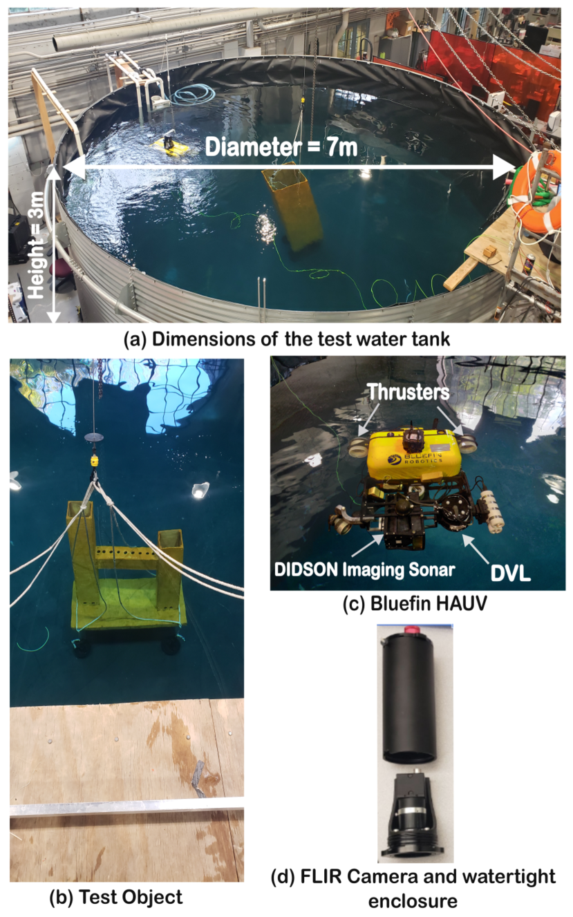
Figure 6: Experimental hardware setup. (a) Test water tank used to conduct the experiments and its dimensions. (b) Test object. (c) Bluefin Hovering Autonomous Underwater Vehicle (HAUV) and its mounted hardware (Didson imaging sonar and Doppler Velocity Log (DVL). (d) FLIR Blackfly S GigE camera used for image capture and its watertight enclosure.

6.2 Results on Experimentally-Captured Data

We also perform real-world experiments on an object (Fig. 6b) submerged in a water tank (Fig. 6a). Please check the supplementary video for more visualizations of the setup. We used a SoundMetrics DIDSON imaging sonar mounted on a Bluefin Hovering Autonomous Underwater Vehicle (HAUV) (Fig. 6c) to capture two sonar datasets of the test object with two different elevation apertures $14^{\circ}$ and $28^{\circ}$. The vehicle uses an IMU and a Doppler Velocity Log (DVL) to measure sonar pose information. We asynchronously capture optical images of the same object using a FLIR Blackfly S GigE 5MP camera (Fig. 6d) with camera pose information computed with COLMAP. The sonar and camera trajectories were aligned post-capture. Similar to the simulation setup, both camera and sonar followed an approximately $1.2m$ non-degenerate linear trajectory, which we later sub-sampled into the same $5$ baselines. We benchmarked our method against three algorithms: The COLMAP based sensor fusion method introduced in [20], NeuS [46], and NeuSIS [39]. For each dataset and sensor baseline, we executed each method six times with randomly initialized seeds except that of  [20], which is deterministic.

Qualitatively, we observe in Fig. 10 that AONeuS outputs a more complete shape across baselines compared to sonar-only (NeuSIS) and camera-only (NeuS) only methods: the hole, two legs, and crossbar are clearly discernible. Conversely, when using only sonar, parts of the object are not well reconstructed as we can observe, for example, with the long leg with NeuSIS at $14^{\circ}$. Similarly, camera-only methods result in the loss of features such as the hole accompanied with significant introduced depth errors. We quantify the results in Tab. 2, where we report the mean and variance of the Chamfer $L_{1}$ distance, precision, and recall against the ground truth mesh computed over six trials with different random seeds for training. We observe that the fusion of the acoustic and optical signals generates higher quality reconstruction, even with very short baselines measuring only 24, as indicated by the mean value of each metric. When comparing AONeus with sonar-only methods (NeuSIS), we note that, despite the increased elevation ambiguity introduced by the $28^{\circ}$ elevation aperture, our technique is able to leverage camera information and its constraints in the $x$ and $y$ axes to resolve spatial locations that are otherwise under-constrained when solely relying on sonar. Techniques that rely on a camera only (NeuS) exhibit a decrease in performance as the sensor baseline is reduced. Complementing camera with sonar information introduces constraints in the depth direction easing the resolution of depth which is known to be difficult to resolve with limited camera motion. We additionally emphasize the variance of the reconstruction quality as measured by the variance of the Chamfer distance: the fusion of both modalities result in outputs that are more robust to the randomness of the algorithm (i.e. network initialization, point samples, etc.).

7 Discussion and Analysis

7.1 Distribution of per-Axis Errors

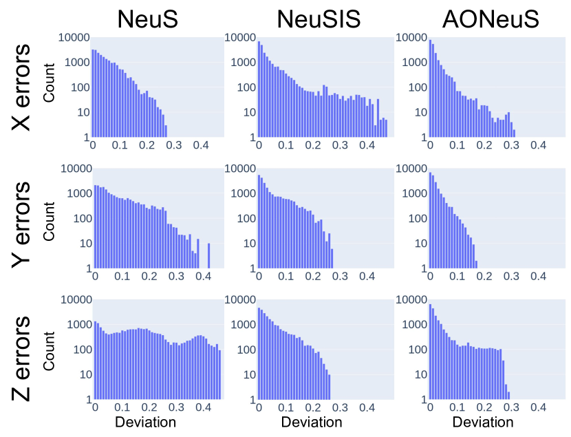
Figure 7: Per-axis error distributions. At 0.2x baseline for the turtle example, we plot the distributions of deviations from the ground truth mesh along all three axes for NeuS, NeuSIS, and AONeuS reconstructions. The NeuS reconstruction has larger $Z$ errors, noticeable from the long tail, where as NeuSIS reconstruction has larger $X$ errors. AONeuS has tighter distributions along all three axes compared to NeuS or NeuSIS showing that the proposed technique takes the best of both of the imaging modalities.

In Fig. 7, we visualize the per-axis deviations from the ground truth for the synthetic turtle scene at 0.24 m baseline. We compute per-axis deviations by first determining the closest vertex in the dense ground truth mesh and taking absolute differences in x, y, and z coordinates. We histogram these deviations along all three axes and show them along rows in the Fig. 7. We have repeated this procedure for NeuS, NeuSIS, and AONeuS and show them along the columns.

From the data, we can observe (1) NeuS has large deviations along $Z$ axes, (2) NeuSIS has large deviations along $X$ axes. These results are consistent with the ambiguities associated with their respective measurement processes. AONeuS has low spread on all axes as it captures the best of both camera (NeuS) and sonar (NeuSIS) imaging modalities.

7.2 Multimodal Sensing is Better Conditioned

The strong empirical performance of our multimodal reconstructions can be explained in terms of system conditioning. Given point correspondences between measurements, it is far easier to triangulate a point using multimodal acoustic-optical measurements than camera-only or sonar-only measurements.

To illustrate this fact, consider a point $P=[X,Y,Z]^{t}$ that is observed by an acoustic-optical sensor from two positions. The sonar’s azimuthal plane is the $yz$ plane, in its own coordinate system. The camera’s image plane is the $z=f$ plane, in its own coordinate system. Without loss of generality, assume the sensor’s coordinate system at its initial location is the world coordinate system and its coordinate system at its second position is described by a rotation $\mathbf{R}$ and translation $\mathbf{t}=[t_{x},t_{y},t_{z}]$. That is, the coordinate of point $P$ in the new coordinate system is $P^{\prime}=\mathbf{R}P+\mathbf{t}$.

Under this model, the acoustic-optical sensor records 8 measurements:

$$x_{c}=f\frac{[1,0,0]P}{[0,0,1]P}, y_{c}=f\frac{[0,1,0]P}{[0,0,1]P},$$

$$R=\|P\|, \theta=\tan^{-1}{\Big{(}}\frac{[0,1,0]P}{[0,0,1]P}{\Big{)}},$$

$$x_{c}^{\prime}=f\frac{\mathbf{r}_{1}^{t}P+t_{x}}{\mathbf{r}_{3}^{t}P+t_{z}}, y_{c}^{\prime}=f\frac{\mathbf{r}_{2}^{t}P+t_{y}}{\mathbf{r}_{3}^{t}P+t_{z}},$$

$$R^{\prime}=\sqrt{\|R\|^{2}+\|t\|^{2}+2\mathbf{t}^{t}\mathbf{R}P}, \theta^{\prime}=\tan^{-1}{\Big{(}}\frac{\mathbf{r}_{2}^{t}P+t_{y}}{\mathbf{r}_{3}^{t}P+t_{z}}{\Big{)}},$$ (13)

where $\mathbf{r_{i}}$ denotes the $i^{th}$ row of $\mathbf{R}$.

Loosely following Negahdaripour et al. [34], Negahdaripour [33], we can turn each of these measurements into seven linear constraints and one non-linear constraint on $P$.

$$\mathbf{A}_{multi}P =b\text{ and }\|P\|^{2}=R^{2}\text{ with }$$

$$\mathbf{A}_{multi} =\begin{bmatrix}(-f,0,x_{c})\\ (0,-f,y_{c})\\ (0,-1,\tan(\theta))\\ x_{c}^{\prime}\mathbf{r}_{3}^{t}-f\mathbf{r}_{2}^{t}\\ y_{c}^{\prime}\mathbf{r}_{3}^{t}-f\mathbf{r}_{2}^{t}\\ \tan(\theta^{\prime})\mathbf{r}_{3}^{t}-\mathbf{r}_{2}^{t}\\ \mathbf{t}^{t}\mathbf{R}\end{bmatrix}\text{ and }b=\begin{bmatrix}0\\ 0\\ 0\\ ft_{x}-x_{c}^{\prime}t_{z}\\ ft_{y}-y_{c}^{\prime}t_{z}\\ t_{y}-\tan(\theta^{\prime})t_{z}\\ \frac{(R^{\prime})^{2}-R^{2}-\|\mathbf{t}\|^{2}}{2}\end{bmatrix}.$$ (14)

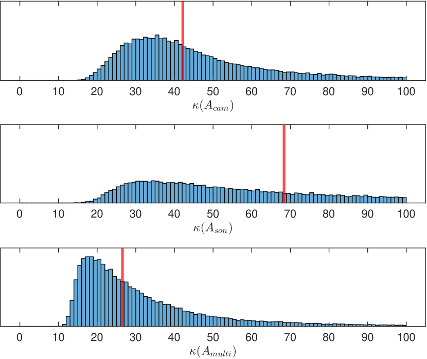
Figure 8: System Conditioning. Histograms of the condition numbers of the camera-only (top), sonar-only (middle), and multimodal (bottom) forward models. Median condition numbers are highlighted in red. The acoustic-optical multimodal forward model is generally better conditioned and easier to invert (triangulation).

One can similarly form camera-only, $\mathbf{A}_{cam}$, and sonar-only, $\mathbf{A}_{son}$, forward models by considering only rows 1, 2, 4, and 5 and rows 3, 6, and 7, respectively, of $\mathbf{A}_{multi}$. By inverting these systems, one can triangulate $P$ in space.

Here we perform Monte Carlo sampling to compare the conditioning of $\mathbf{A}_{cam}$, $\mathbf{A}_{son}$, and $\mathbf{A}_{multi}$. We sample $P$ uniformly in a 1 $m^{3}$ cube centered at $(0,0,1.5)$ with edges parallel to the $x$, $y$, and $z$ axis; we assume $f=\qty{100}{\milli}$; we sample $t_{x}$, $t_{y}$, and $t_{z}$ uniformly in the range $\qty{0}{\centi}$ to $\qty{10}{\centi}$; and we sample the yaw, pitch, and roll between measurements uniformly in the range -5 to 5 .

For each realization of these parameters, we compute the condition number, $\kappa$, of $\mathbf{A}_{cam}$, $\mathbf{A}_{son}$, and $\mathbf{A}_{multi}$. We repeat this process $50,000$ times to form histograms, illustrated in Fig. 8. The condition number of the multimodal system is generally much lower and the system is thus easier to invert; multimodal triangulation is easier.

8 Conclusion

We have introduced and validated a multimodal inverse-differentiable-rendering framework for reconstructing 3D surface information from camera and sonar measurements. Our framework combines camera and sonar information using a unified surface representation module and separate modality-specific appearance modules and rendering functions. By extracting information from these complementary modalities, our framework is able to offer breakthrough underwater sensing capabilities for restricted baseline imaging scenarios. We have demonstrated that AONeuS can accurately reconstruct the geometry of complex 3D objects from synthetic as well as noisy, real-world measurements captured over severely restricted baselines.

While we demonstrate the first neural fusion of camera and sonar measurements, there are many interesting directions to explore this amalgamation. In Sec. 5.1.2, we introduced a heuristic for weighing camera and sonar measurements. A structured way of combining the camera and sonar data, which is aware of the uncertainties [19, 17] in the complementary imaging systems could result in faster convergence rates and better reconstructions.

The sonar we have used in our implementations are forward-looking sonars. Fusion algorithms for side-scan sonars, synthetic-aperture sonars, sonars of different ranges and wavelengths, could be an interesting forward direction. Similarly, extending the technique for various geometries and materials including multi-object scenes, dynamic scenes, cluttered scenes and scattering media (murky water) would make AONeuS more practical. Finally, on-the-fly reconstructions could allow one to select the best next underwater view to improve reconstruction accuracy and further reduce the required baseline and acquisition time.

9 Acknowledgements

The authors would like to thank Tianxiang Lin and Jui-Te Huang for their help with data collection and Sarah Friday for providing an animation showcasing the real experimental setup. M.Q., A.H., and M.K. were supported in part by ONR grant N00014-21-1-2482. A.P. was supported by NSF grant 2326904. K.Z. and C.A.M. were supported in part by AFOSR Young Investigator Program award no. FA9550-22-1-0208, ONR award no. N00014-23-1-2752, and a seed grant from SAAB, Inc.

				Sonar dataset 1 $14^{\circ}$ elevation angle		Sonar dataset 2 $28^{\circ}$ elevation angle
Baseline	Metric	NeuS	Kim et al. (2019)	NeuSIS ($14^{\circ}$)	AONeuS ($14^{\circ}$)	NeuSIS ($28^{\circ}$)	AONeuS ($28^{\circ}$)
1.2m	Chamfer L1 $\boldsymbol{\downarrow}$	$\mathbf{0.092}\pm 0.015$	0.177	$0.187\pm 0.032$	$0.093\pm 0.005$	$0.217\pm 0.036$	$0.105\pm 0.008$
	Precision $\boldsymbol{\uparrow}$	$\mathbf{0.693}\pm 0.066$	0.336	$0.482\pm 0.063$	$0.661\pm 0.025$	$0.444\pm 0.026$	$0.602\pm 0.023$
	Recall $\boldsymbol{\uparrow}$	$0.679\pm 0.098$	0.387	$0.355\pm 0.051$	$\mathbf{0.707}\pm 0.047$	$0.318\pm 0.040$	$0.614\pm 0.037$
0.96m	Chamfer L1 $\boldsymbol{\downarrow}$	$0.107\pm 0.013$	0.182	$0.180\pm 0.026$	$\mathbf{0.095}\pm 0.008$	$0.214\pm 0.032$	$0.097\pm 0.006$
	Precision $\boldsymbol{\uparrow}$	$0.661\pm 0.048$	0.318	$0.514\pm 0.036$	$\mathbf{0.689}\pm 0.042$	$0.462\pm 0.032$	$0.645\pm 0.038$
	Recall $\boldsymbol{\uparrow}$	$0.563\pm 0.084$	0.345	$0.370\pm 0.053$	$\mathbf{0.695}\pm 0.037$	$0.314\pm 0.043$	$0.648\pm 0.038$
0.72m	Chamfer L1 $\boldsymbol{\downarrow}$	$0.127\pm 0.013$	0.178	$0.174\pm 0.034$	$\mathbf{0.094}\pm 0.008$	$0.202\pm 0.043$	$0.095\pm 0.010$
	Precision $\boldsymbol{\uparrow}$	$\mathbf{0.651}\pm 0.047$	0.368	$0.550\pm 0.080$	$0.646\pm 0.035$	$0.502\pm 0.063$	$0.640\pm 0.037$
	Recall $\boldsymbol{\uparrow}$	$0.500\pm 0.062$	0.396	$0.374\pm 0.061$	$\mathbf{0.698}\pm 0.067$	$0.352\pm 0.065$	$0.668\pm 0.073$
0.48m	Chamfer L1 $\boldsymbol{\downarrow}$	$0.150\pm 0.022$	0.179	$0.180\pm 0.032$	$\mathbf{0.097}\pm 0.012$	$0.215\pm 0.034$	$0.098\pm 0.010$
	Precision $\boldsymbol{\uparrow}$	$0.626\pm 0.055$	0.324	$0.521\pm 0.050$	$\mathbf{0.656}\pm 0.065$	$0.473\pm 0.037$	$0.607\pm 0.050$
	Recall $\boldsymbol{\uparrow}$	$0.415\pm 0.022$	0.218	$0.372\pm 0.065$	$\mathbf{0.678}\pm 0.075$	$0.336\pm 0.061$	$0.653\pm 0.063$
0.24m	Chamfer L1 $\boldsymbol{\downarrow}$	$0.167\pm 0.012$	0.198	$0.173\pm 0.020$	$\mathbf{0.087}\pm 0.007$	$0.203\pm 0.023$	$0.089\pm 0.007$
	Precision $\boldsymbol{\uparrow}$	$0.580\pm 0.031$	0.305	$0.535\pm 0.063$	$\mathbf{0.699}\pm 0.057$	$0.501\pm 0.021$	$0.651\pm 0.049$
	Recall $\boldsymbol{\uparrow}$	$0.363\pm 0.056$	0.140	$0.347\pm 0.030$	$\mathbf{0.760}\pm 0.030$	$0.317\pm 0.024$	$0.705\pm 0.037$

Table 2: For the hardware reconstruction of ”H” object in Fig. 10, we report the mean and standard deviation of the Chamfer L1 distance, precision, and recall compared to the ground truth (obtained from a laser scan of the real structure) for various reconstruction techniques. We computed the standard deviation over 6 trials. For metric calculation, we used a threshold of 0.05m.

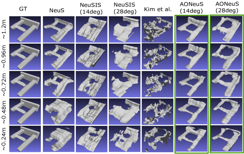
Figure 10: Experimental Results with “h” Object. As the baseline diminishes, NeuS exhibits increasing amount of distortion along the depth direction as can seen at the intersection of the short piling and crossbar at the 0.72m and 0.96m baselines. NeuSIS similarly generates reconstructions with significant errors (for example, the long piling is poorly reconstructed with the $14^{\circ}$ elevation). Conversely, AONeuS consistently produces faithful reconstructions across a range of baselines.

9.1 Variance of the Density Field Over Realizations of the Algorithm

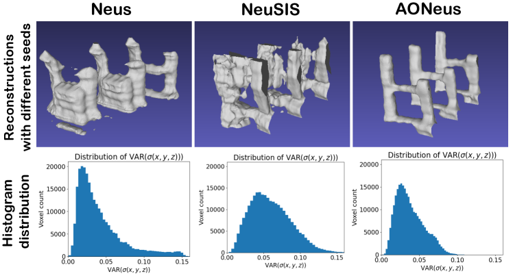
Figure 11: Distribution of Reconstructions of the Real Object. Top: Different Reconstructions from different random seeds for the 20% baseline. Bottom: Histogram distribution of the variance of the density field VAR($\sigma(\mathbf{x})$) vs. voxel count. Neus’s distribution is heavily tailed while NeuSIS’s distribution exhibits a large mean and variance. AONeuS’s distribution is light-tailed with a small mean and therefore it is better constrained.

9.2 Additional tables

Tables 3 to 6 provide additional quantitative metrics for our synthetic experiments.

		NeuS	NeuSIS	AONeuS
1.2m	Chamfer $\boldsymbol{\downarrow}$	$\mathbf{0.112}\pm 0.018$	$0.197\pm 0.011$	$0.117\pm 0.014$
	Precision $\boldsymbol{\uparrow}$	$\mathbf{0.652}\pm 0.058$	$0.295\pm 0.019$	$0.582\pm 0.053$
	Recall $\boldsymbol{\uparrow}$	$0.650\pm 0.044$	$0.643\pm 0.025$	$\mathbf{0.741}\pm 0.028$
0.96m	Chamfer $\boldsymbol{\downarrow}$	$0.144\pm 0.021$	$0.200\pm 0.019$	$\mathbf{0.134}\pm 0.016$
	Precision $\boldsymbol{\uparrow}$	$0.559\pm 0.045$	$0.291\pm 0.014$	$\mathbf{0.575}\pm 0.017$
	Recall $\boldsymbol{\uparrow}$	$0.579\pm 0.042$	$0.650\pm 0.043$	$\mathbf{0.697}\pm 0.027$
0.72m	Chamfer $\boldsymbol{\downarrow}$	$0.146\pm 0.021$	$0.200\pm 0.016$	$\mathbf{0.141}\pm 0.023$
	Precision $\boldsymbol{\uparrow}$	$0.554\pm 0.052$	$0.289\pm 0.029$	$\mathbf{0.558}\pm 0.035$
	Recall $\boldsymbol{\uparrow}$	$0.599\pm 0.039$	$0.629\pm 0.067$	$\mathbf{0.689}\pm 0.048$
0.48m	Chamfer $\boldsymbol{\downarrow}$	$0.174\pm 0.016$	$0.199\pm 0.012$	$\mathbf{0.146}\pm 0.033$
	Precision $\boldsymbol{\uparrow}$	$0.468\pm 0.039$	$0.287\pm 0.047$	$\mathbf{0.533}\pm 0.087$
	Recall $\boldsymbol{\uparrow}$	$0.516\pm 0.040$	$0.569\pm 0.076$	$\mathbf{0.668}\pm 0.044$
0.24m	Chamfer $\boldsymbol{\downarrow}$	$0.223\pm 0.046$	$0.182\pm 0.011$	$\mathbf{0.166}\pm 0.034$
	Precision $\boldsymbol{\uparrow}$	$0.341\pm 0.090$	$0.358\pm 0.042$	$\mathbf{0.451}\pm 0.103$
	Recall $\boldsymbol{\uparrow}$	$0.413\pm 0.072$	$0.555\pm 0.069$	$\mathbf{0.644}\pm 0.045$

Table 3: Quantitative metrics for the airplane mesh.

		NeuS	NeuSIS	AONeuS
1.2m	Chamfer $\boldsymbol{\downarrow}$	$0.147\pm 0.017$	$0.187\pm 0.012$	$\mathbf{0.105}\pm 0.019$
	Precision $\boldsymbol{\uparrow}$	$0.448\pm 0.073$	$0.328\pm 0.020$	$\mathbf{0.592}\pm 0.110$
	Recall $\boldsymbol{\uparrow}$	$0.454\pm 0.100$	$0.460\pm 0.037$	$\mathbf{0.626}\pm 0.090$
0.96m	Chamfer $\boldsymbol{\downarrow}$	$0.167\pm 0.027$	$0.203\pm 0.014$	$\mathbf{0.142}\pm 0.074$
	Precision $\boldsymbol{\uparrow}$	$0.394\pm 0.070$	$0.302\pm 0.025$	$\mathbf{0.534}\pm 0.230$
	Recall $\boldsymbol{\uparrow}$	$\mathbf{0.398}\pm 0.106$	$0.445\pm 0.033$	$0.533\pm 0.228$
0.72m	Chamfer $\boldsymbol{\downarrow}$	$0.191\pm 0.019$	$0.225\pm 0.030$	$\mathbf{0.128}\pm 0.021$
	Precision $\boldsymbol{\uparrow}$	$0.357\pm 0.053$	$0.275\pm 0.040$	$\mathbf{0.533}\pm 0.112$
	Recall $\boldsymbol{\uparrow}$	$0.417\pm 0.077$	$0.390\pm 0.040$	$\mathbf{0.576}\pm 0.105$
0.48m	Chamfer $\boldsymbol{\downarrow}$	$0.237\pm 0.039$	$0.243\pm 0.019$	$\mathbf{0.143}\pm 0.015$
	Precision $\boldsymbol{\uparrow}$	$0.321\pm 0.062$	$0.257\pm 0.012$	$\mathbf{0.523}\pm 0.069$
	Recall $\boldsymbol{\uparrow}$	$0.392\pm 0.091$	$0.370\pm 0.017$	$\mathbf{0.577}\pm 0.043$
0.24m	Chamfer $\boldsymbol{\downarrow}$	$0.293\pm 0.044$	$0.272\pm 0.055$	$\mathbf{0.186}\pm 0.034$
	Precision $\boldsymbol{\uparrow}$	$0.251\pm 0.049$	$0.225\pm 0.039$	$\mathbf{0.440}\pm 0.116$
	Recall $\boldsymbol{\uparrow}$	$0.277\pm 0.103$	$0.290\pm 0.076$	$\mathbf{0.483}\pm 0.130$

Table 4: Quantitative metrics for the lobster mesh.

		NeuS	NeuSIS	AONeuS
1.2m	Chamfer $\boldsymbol{\downarrow}$	$0.108\pm 0.020$	$0.177\pm 0.010$	$\mathbf{0.088}\pm 0.022$
	Precision $\boldsymbol{\uparrow}$	$0.585\pm 0.070$	$0.335\pm 0.021$	$\mathbf{0.714}\pm 0.106$
	Recall $\boldsymbol{\uparrow}$	$0.722\pm 0.061$	$\mathbf{0.894}\pm 0.031$	$0.886\pm 0.026$
0.96m	Chamfer $\boldsymbol{\downarrow}$	$0.122\pm 0.030$	$0.170\pm 0.014$	$\mathbf{0.089}\pm 0.016$
	Precision $\boldsymbol{\uparrow}$	$0.539\pm 0.117$	$0.352\pm 0.032$	$\mathbf{0.720}\pm 0.063$
	Recall $\boldsymbol{\uparrow}$	$0.689\pm 0.122$	$\mathbf{0.848}\pm 0.022$	$0.829\pm 0.033$
0.72m	Chamfer $\boldsymbol{\downarrow}$	$0.159\pm 0.035$	$0.171\pm 0.010$	$\mathbf{0.126}\pm 0.035$
	Precision $\boldsymbol{\uparrow}$	$0.435\pm 0.089$	$0.352\pm 0.033$	$\mathbf{0.571}\pm 0.118$
	Recall $\boldsymbol{\uparrow}$	$0.550\pm 0.127$	$\mathbf{0.791}\pm 0.026$	$0.764\pm 0.092$
0.48m	Chamfer $\boldsymbol{\downarrow}$	$0.255\pm 0.041$	$0.170\pm 0.006$	$\mathbf{0.143}\pm 0.046$
	Precision $\boldsymbol{\uparrow}$	$0.175\pm 0.059$	$0.372\pm 0.019$	$\mathbf{0.486}\pm 0.121$
	Recall $\boldsymbol{\uparrow}$	$0.201\pm 0.081$	$\mathbf{0.742}\pm 0.039$	$0.657\pm 0.080$
0.24m	Chamfer $\boldsymbol{\downarrow}$	$0.548\pm 0.144$	$\mathbf{0.191}\pm 0.006$	$0.196\pm 0.033$
	Precision $\boldsymbol{\uparrow}$	$0.067\pm 0.038$	$0.344\pm 0.023$	$\mathbf{0.377}\pm 0.088$
	Recall $\boldsymbol{\uparrow}$	$0.071\pm 0.045$	$\mathbf{0.627}\pm 0.069$	$0.516\pm 0.072$

Table 5: Quantitative metrics for the seastar mesh.

		NeuS	NeuSIS	AONeuS
1.2m	Chamfer $\boldsymbol{\downarrow}$	$\mathbf{0.063}\pm 0.002$	$0.077\pm 0.010$	$0.066\pm 0.006$
	Precision $\boldsymbol{\uparrow}$	$0.847\pm 0.011$	$0.754\pm 0.066$	$\mathbf{0.858}\pm 0.024$
	Recall $\boldsymbol{\uparrow}$	$\mathbf{0.941}\pm 0.018$	$0.814\pm 0.035$	$0.844\pm 0.038$
0.96m	Chamfer $\boldsymbol{\downarrow}$	$\mathbf{0.068}\pm 0.005$	$0.078\pm 0.012$	$0.078\pm 0.006$
	Precision $\boldsymbol{\uparrow}$	$\mathbf{0.833}\pm 0.023$	$0.756\pm 0.072$	$0.816\pm 0.022$
	Recall $\boldsymbol{\uparrow}$	$\mathbf{0.929}\pm 0.020$	$0.803\pm 0.043$	$0.794\pm 0.031$
0.72m	Chamfer $\boldsymbol{\downarrow}$	$\mathbf{0.078}\pm 0.006$	$0.091\pm 0.016$	$0.090\pm 0.006$
	Precision $\boldsymbol{\uparrow}$	$0.769\pm 0.035$	$0.747\pm 0.086$	$\mathbf{0.774}\pm 0.029$
	Recall $\boldsymbol{\uparrow}$	$\mathbf{0.876}\pm 0.044$	$0.746\pm 0.075$	$0.730\pm 0.021$
0.48m	Chamfer $\boldsymbol{\downarrow}$	$0.107\pm 0.014$	$0.107\pm 0.017$	$\mathbf{0.098}\pm 0.009$
	Precision $\boldsymbol{\uparrow}$	$0.620\pm 0.064$	$\mathbf{0.791}\pm 0.077$	$0.714\pm 0.031$
	Recall $\boldsymbol{\uparrow}$	$0.690\pm 0.084$	$0.676\pm 0.078$	$\mathbf{0.691}\pm 0.037$
0.24m	Chamfer $\boldsymbol{\downarrow}$	$0.199\pm 0.029$	$0.168\pm 0.008$	$\mathbf{0.109}\pm 0.010$
	Precision $\boldsymbol{\uparrow}$	$0.309\pm 0.028$	$\mathbf{0.832}\pm 0.041$	$0.667\pm 0.048$
	Recall $\boldsymbol{\uparrow}$	$0.302\pm 0.029$	$0.465\pm 0.032$	$\mathbf{0.640}\pm 0.047$

Table 6: Quantitative metrics for the shell mesh.

References

- Albiez et al. [2015] Jan Albiez, Sylvain Joyeux, Christopher Gaudig, Jens Hilljegerdes, Sven Kroffke, Christian Schoo, Sascha Arnold, Geovane Mimoso, Pedro Alcantara, Rafael Saback, et al. Flatfish-a compact subsea-resident inspection auv. In OCEANS 2015-MTS/IEEE Washington, pages 1–8, 201 Waterfront Street National Harbor, Maryland 20745 USA, 2015. IEEE, IEEE.
- Andrea et al. [2023] Ramazzina Andrea, Bijelic Mario, Walz Stefanie, Sanvito Alessandro, Scheuble Dominik, and Heide Felix. Scatternerf: Seeing through fog with physically-based inverse neural rendering. 2023.
- Arnold and Wehbe [2022] Sascha Arnold and Bilal Wehbe. Spatial acoustic projection for 3d imaging sonar reconstruction. In 2022 International Conference on Robotics and Automation (ICRA), pages 3054–3060, Philadelphia, 2022. IEEE.
- Attal et al. [2021] Benjamin Attal, Eliot Laidlaw, Aaron Gokaslan, Changil Kim, Christian Richardt, James Tompkin, and Matthew O’Toole. Törf: Time-of-flight radiance fields for dynamic scene view synthesis. Advances in Neural Information Processing Systems, 34, 2021.
- Aykin and Negahdaripour [2015] Murat D Aykin and Shahriar Negahdaripour. On 3-d target reconstruction from multiple 2-d forward-scan sonar views. In OCEANS 2015-Genova, pages 1–10. IEEE, 2015.
- Aykin and Negahdaripour [2016a] Murat D Aykin and Shahriar Negahdaripour. Three-dimensional target reconstruction from multiple 2-d forward-scan sonar views by space carving. IEEE Journal of Oceanic Engineering, 42(3):574–589, 2016a.
- Aykin and Negahdaripour [2016b] Murat D Aykin and Shahriar S Negahdaripour. Modeling 2-d lens-based forward-scan sonar imagery for targets with diffuse reflectance. IEEE journal of oceanic engineering, 41(3):569–582, 2016b.
- Babaee and Negahdaripour [2015] Mohammadreza Babaee and Shahriar Negahdaripour. 3-d object modeling from 2-d occluding contour correspondences by opti-acoustic stereo imaging. Computer Vision and Image Understanding, 132:56–74, 2015.
- Bernardini et al. [1999] Fausto Bernardini, Joshua Mittleman, Holly Rushmeier, Cláudio Silva, and Gabriel Taubin. The ball-pivoting algorithm for surface reconstruction. IEEE transactions on visualization and computer graphics, 5(4):349–359, 1999.
- Bijelic et al. [2020] Mario Bijelic, Tobias Gruber, Fahim Mannan, Florian Kraus, Werner Ritter, Klaus Dietmayer, and Felix Heide. Seeing through fog without seeing fog: Deep multimodal sensor fusion in unseen adverse weather. In Proceedings of the IEEE/CVF Conference on Computer Vision and Pattern Recognition, pages 11682–11692, 2020.
- Carlson et al. [2023] Alexandra Carlson, Manikandasriram S. Ramanagopal, Nathan Tseng, Matthew Johnson-Roberson, Ram Vasudevan, and Katherine A. Skinner. Cloner: Camera-lidar fusion for occupancy grid-aided neural representations. IEEE Robotics and Automation Letters, 8(5):2812–2819, 2023.
- Chen et al. [2024] W. Chen, W. Yifan, S. Kuo, and G. Wetzstein. Dehazenerf: Multiple image haze removal and 3d shape reconstruction using neural radiance fields. In 3DV, 2024.
- Community [2022] Blender Online Community. Blender - a 3D modelling and rendering package. Blender Foundation, Stichting Blender Foundation, Amsterdam, 2022.
- Dave et al. [2022] Akshat Dave, Yongyi Zhao, and Ashok Veeraraghavan. PANDORA: Polarization-Aided Neural Decomposition of Radiance, page 538–556. Springer Nature Switzerland, 2022.
- DeBortoli et al. [2019] Robert DeBortoli, Fuxin Li, and Geoffrey A Hollinger. Elevatenet: A convolutional neural network for estimating the missing dimension in 2d underwater sonar images. In 2019 IEEE/RSJ International Conference on Intelligent Robots and Systems (IROS), pages 8040–8047. IEEE, 2019.
- Ferreira et al. [2016] Fausto Ferreira, Diogo Machado, Gabriele Ferri, Samantha Dugelay, and John Potter. Underwater optical and acoustic imaging: A time for fusion? a brief overview of the state-of-the-art. OCEANS 2016 MTS/IEEE Monterey, pages 1–6, 2016.
- Goli et al. [2023] Lily Goli, Cody Reading, Silvia Sellán, Alec Jacobson, and Andrea Tagliasacchi. Bayes’ Rays: Uncertainty quantification in neural radiance fields. arXiv preprint arXiv:2309.03185, 2023.
- Jaffe [2014] Jules S Jaffe. Underwater optical imaging: the past, the present, and the prospects. IEEE Journal of Oceanic Engineering, 40(3):683–700, 2014.
- Jiang et al. [2023] Wen Jiang, Boshu Lei, and Kostas Daniilidis. Fisherrf: Active view selection and uncertainty quantification for radiance fields using fisher information. arXiv preprint arXiv:2311.17874, 2023.
- Kim et al. [2019] Jason Kim, Meungsuk Lee, Seokyong Song, Byeongjin Kim, and Son-Cheol Yu. 3-D Reconstruction of Underwater Objects Using Image Sequences from Optical Camera and Imaging Sonar. In OCEANS 2019 MTS/IEEE SEATTLE, pages 1–6, 2019.
- Kim et al. [2023] Youngchan Kim, Wonjoon Jin, Sunghyun Cho, and Seung-Hwan Baek. Neural spectro-polarimetric fields. In SIGGRAPH Asia 2023 Conference Papers, New York, NY, USA, 2023. Association for Computing Machinery.
- Kim et al. [2009] Young Min Kim, Christian Theobalt, James Diebel, Jana Kosecka, Branislav Miscusik, and Sebastian Thrun. Multi-view image and tof sensor fusion for dense 3d reconstruction. In 2009 IEEE 12th International Conference on Computer Vision Workshops, ICCV Workshops, pages 1542–1549, 2009.
- Lensgraf et al. [2021] Samuel Lensgraf, Amy Sniffen, Zachary Zitzewitz, Evan Honnold, Jennifer Jain, Weifu Wang, Alberto Li, and Devin Balkcom. Droplet: Towards autonomous underwater assembly of modular structures. In Proceedings of Robotics: Science and Systems, 2021.
- Levy et al. [2023] Deborah Levy, Amit Peleg, Naama Pearl, Dan Rosenbaum, Derya Akkaynak, Simon Korman, and Tali Treibitz. Seathru-nerf: Neural radiance fields in scattering media. In Proceedings of the IEEE/CVF Conference on Computer Vision and Pattern Recognition, pages 56–65, 2023.
- Lin et al. [2023] Tianxiang Lin, Akshay Hinduja, Mohamad Qadri, and Michael Kaess. Conditional gans for sonar image filtering with applications to underwater occupancy mapping. In 2023 IEEE International Conference on Robotics and Automation (ICRA), pages 1048–1054. IEEE, 2023.
- Lindell et al. [2018] David B. Lindell, Matthew O’Toole, and Gordon Wetzstein. Single-Photon 3D Imaging with Deep Sensor Fusion. ACM Trans. Graph. (SIGGRAPH), (4), 2018.
- Liu et al. [2023a] Afei Liu, Shuanghui Zhang, Chi Zhang, Shuaifeng Zhi, and Xiang Li. Ranerf: Neural 3-d reconstruction of space targets from isar image sequences. IEEE Transactions on Geoscience and Remote Sensing, 61:1–15, 2023a.
- Liu et al. [2023b] Haowen Liu, Monika Roznere, and Alberto Quattrini Li. Deep underwater monocular depth estimation with single-beam echosounder. In 2023 IEEE International Conference on Robotics and Automation (ICRA), pages 1090–1097. IEEE, 2023b.
- Long et al. [2022] Xiaoxiao Long, Cheng Lin, Peng Wang, Taku Komura, and Wenping Wang. Sparseneus: Fast generalizable neural surface reconstruction from sparse views. ECCV, 2022.
- Malik et al. [2023] Anagh Malik, Parsa Mirdehghan, Sotiris Nousias, Kiriakos N. Kutulakos, and David B. Lindell. Transient neural radiance fields for lidar view synthesis and 3d reconstruction. NeurIPS, 2023.
- Menna et al. [2018] Fabio Menna, Panagiotis Agrafiotis, and Andreas Georgopoulos. State of the art and applications in archaeological underwater 3d recording and mapping. Journal of Cultural Heritage, 33:231–248, 2018.
- Mildenhall et al. [2020] Ben Mildenhall, Pratul P. Srinivasan, Matthew Tancik, Jonathan T. Barron, Ravi Ramamoorthi, and Ren Ng. Nerf: Representing scenes as neural radiance fields for view synthesis. In ECCV, 2020.
- Negahdaripour [2018] Shahriar Negahdaripour. Application of forward-scan sonar stereo for 3-d scene reconstruction. IEEE journal of oceanic engineering, 45(2):547–562, 2018.
- Negahdaripour et al. [2009] Shahriar Negahdaripour, Hicham Sekkati, and Hamed Pirsiavash. Opti-acoustic stereo imaging: On system calibration and 3-d target reconstruction. IEEE Transactions on image processing, 18(6):1203–1214, 2009.
- Negahdaripour et al. [2017] Shahriar Negahdaripour, Victor M Milenkovic, Nikan Salarieh, and Mahsa Mirzargar. Refining 3-d object models constructed from multiple fs sonar images by space carving. In OCEANS 2017-Anchorage, pages 1–9. IEEE, 2017.
- Nishimura et al. [2020] Mark Nishimura, David B Lindell, Christopher Metzler, and Gordon Wetzstein. Disambiguating monocular depth estimation with a single transient. In European Conference on Computer Vision, pages 139–155. Springer, 2020.
- Oechsle et al. [2021] Michael Oechsle, Songyou Peng, and Andreas Geiger. Unisurf: Unifying neural implicit surfaces and radiance fields for multi-view reconstruction. In International Conference on Computer Vision (ICCV), 2021.
- Poggi et al. [2022] Matteo Poggi, Pierluigi Zama Ramirez, Fabio Tosi, Samuele Salti, Luigi Di Stefano, and Stefano Mattoccia. Cross-spectral neural radiance fields. In Proceedings of the International Conference on 3D Vision, 2022. 3DV.
- Qadri et al. [2023] Mohamad Qadri, Michael Kaess, and Ioannis Gkioulekas. Neural implicit surface reconstruction using imaging sonar. In 2023 IEEE International Conference on Robotics and Automation (ICRA), pages 1040–1047. IEEE, 2023.
- Reed et al. [2023] Albert Reed, Juhyeon Kim, Thomas Blanford, Adithya Pediredla, Daniel Brown, and Suren Jayasuriya. Neural Volumetric Reconstruction for Coherent Synthetic Aperture Sonar. ACM Transactions on Graphics, 42(4):113:1–113:20, 2023.
- Schonberger and Frahm [2016] Johannes L Schonberger and Jan-Michael Frahm. Structure-from-motion revisited. In Proceedings of the IEEE conference on computer vision and pattern recognition, pages 4104–4113, 2016.
- Sethuraman et al. [2023] Advaith Venkatramanan Sethuraman, Manikandasriram Srinivasan Ramanagopal, and Katherine A Skinner. Waternerf: Neural radiance fields for underwater scenes. In OCEANS 2023-MTS/IEEE US Gulf Coast, pages 1–7. IEEE, 2023.
- Teixeira et al. [2016] Pedro V Teixeira, Michael Kaess, Franz S Hover, and John J Leonard. Underwater inspection using sonar-based volumetric submaps. In 2016 IEEE/RSJ International Conference on Intelligent Robots and Systems (IROS), pages 4288–4295. IEEE, 2016.
- Tinh and Khanh [2021] Nguyen Dinh Tinh and T Dang Khanh. A new imaging geometry model for multi-receiver synthetic aperture sonar considering variation of the speed of sound in seawater. IEIE Transactions on Smart Processing and Computing, 10(4):302–308, 2021.
- Wang et al. [2019a] Jinkun Wang, Tixiao Shan, and Brendan Englot. Underwater terrain reconstruction from forward-looking sonar imagery. In 2019 International Conference on Robotics and Automation (ICRA), pages 3471–3477. IEEE, 2019a.
- Wang et al. [2021a] Peng Wang, Lingjie Liu, Yuan Liu, Christian Theobalt, Taku Komura, and Wenping Wang. Neus: Learning neural implicit surfaces by volume rendering for multi-view reconstruction. Advances in Neural Information Processing Systems, 34:27171–27183, 2021a.
- Wang et al. [2018] Yusheng Wang, Yonghoon Ji, Hanwool Woo, Yusuke Tamura, Atsushi Yamashita, and Asama Hajime. 3d occupancy mapping framework based on acoustic camera in underwater environment. IFAC-PapersOnLine, 51(22):324–330, 2018.
- Wang et al. [2019b] Yusheng Wang, Yonghoon Ji, Hanwool Woo, Yusuke Tamura, Atsushi Yamashita, and Hajime Asama. Three-dimensional underwater environment reconstruction with graph optimization using acoustic camera. In 2019 IEEE/SICE International Symposium on System Integration (SII), pages 28–33. IEEE, 2019b.
- Wang et al. [2021b] Yusheng Wang, Yonghoon Ji, Dingyu Liu, Hiroshi Tsuchiya, Atsushi Yamashita, and Hajime Asama. Elevation angle estimation in 2d acoustic images using pseudo front view. IEEE Robotics and Automation Letters, 6(2):1535–1542, 2021b.
- Westman and Kaess [2019] Eric Westman and Michael Kaess. Wide aperture imaging sonar reconstruction using generative models. In 2019 IEEE/RSJ International Conference on Intelligent Robots and Systems (IROS), pages 8067–8074. IEEE, 2019.
- Westman et al. [2020a] Eric Westman, Ioannis Gkioulekas, and Michael Kaess. A theory of fermat paths for 3d imaging sonar reconstruction. In 2020 IEEE/RSJ International Conference on Intelligent Robots and Systems (IROS), pages 5082–5088. IEEE, 2020a.
- Westman et al. [2020b] Eric Westman, Ioannis Gkioulekas, and Michael Kaess. A volumetric albedo framework for 3d imaging sonar reconstruction. In 2020 IEEE International Conference on Robotics and Automation (ICRA), pages 9645–9651. IEEE, 2020b.
- Yariv et al. [2020] Lior Yariv, Yoni Kasten, Dror Moran, Meirav Galun, Matan Atzmon, Basri Ronen, and Yaron Lipman. Multiview neural surface reconstruction by disentangling geometry and appearance. Advances in Neural Information Processing Systems, 33:2492–2502, 2020.
- Yariv et al. [2021] Lior Yariv, Jiatao Gu, Yoni Kasten, and Yaron Lipman. Volume rendering of neural implicit surfaces. In Thirty-Fifth Conference on Neural Information Processing Systems, 2021.
- Yariv et al. [2023] Lior Yariv, Peter Hedman, Christian Reiser, Dor Verbin, Pratul P. Srinivasan, Richard Szeliski, Jonathan T. Barron, and Ben Mildenhall. Bakedsdf: Meshing neural sdfs for real-time view synthesis. arXiv, 2023.
- Zhu et al. [2023] Haidong Zhu, Yuyin Sun, Chi Liu, Lu Xia, Jiajia Luo, Nan Qiao, Ram Nevatia, and Cheng–Hao Kuo. Multimodal neural radiance field. In 2023 IEEE International Conference on Robotics and Automation (ICRA), pages 9393–9399, 2023.