Flora: Low-Rank Adapters
Are Secretly Gradient Compressors

Abstract

Despite large neural networks demonstrating remarkable abilities to complete different tasks, they require excessive memory usage to store the optimization states for training. To alleviate this, the low-rank adaptation (LoRA) is proposed to reduce the optimization states by training fewer parameters. However, LoRA restricts overall weight update matrices to be low-rank, limiting the model performance. In this work, we investigate the dynamics of LoRA and identify that it can be approximated by a random projection. Based on this observation, we propose Flora, which is able to achieve high-rank updates by resampling the projection matrices while enjoying the sublinear space complexity of optimization states. We conduct experiments across different tasks and model architectures to verify the effectiveness of our approach.

1 Introduction

Gradient-based optimization powers the learning part of deep neural networks. In the simplest form, stochastic gradient descent (SGD) updates the model parameters using noisy estimation of the negative gradient. More advanced methods track various gradient statistics to stabilize and accelerate training (Duchi et al., 2011; Hinton et al., 2012). For example, the momentum technique tracks an exponential moving average of gradients for variance reduction (Cutkosky and Orabona, 2019) and damping (Goh, 2017). On the other hand, gradient accumulation computes the average of gradients in the last few batches to simulate a larger effective batch for variance reduction (Wang et al., 2013). Both cases require an additional memory buffer equal to the model size to store the information.

However, such a linear space complexity of optimization states becomes problematic in modern deep learning. For example, GPT-3 (Brown et al., 2020) and Stable Diffusion (Rombach et al., 2022) are trained with Adam (Kingma and Ba, 2015) where momentum is applied. For each scalar in the parameter set, Adam maintains two additional variables (i.e., first- and second-moment estimates), tripling the memory usage. The largest GPT-3, for example, has $175$ billion parameters taking $700$GB of memory. Adam requires an additional $1.4$TB memory for optimization states. This excessive amount of memory usage poses a scaling challenge.

One line of research saves memory by training a subset of parameters (Houlsby et al., 2019; Zaken et al., 2022), so the optimizer only stores information about a small set of trainable parameters. One notable example is the low-rank adaptation (LoRA, Hu et al., 2022). LoRA updates parameter matrices by low-rank patches, which contain much fewer trainable parameters. In this way, the momentum and gradient accumulation also have much smaller sizes. However, LoRA restricts the weight update to be in the low-rank form, limiting the optimization space of the model parameters.

Another line of work designs new optimizers that use less memory (Dettmers et al., 2021; Feinberg et al., 2023). For instance, Adafactor (Shazeer and Stern, 2018) leverages the closed-form solution of generalized Kullback–Leibler divergence (Finesso and Spreij, 2006) to reconstruct the second-moment estimate in Adam. To optimize a matrix in $\mathbb{R}^{n\times m}$, Adafactor reduces the memory from $O(nm)$ to $O(n+m)$, making the space complexity of second-moment estimation sublinear in model size. However, Adafactor drops the momentum technique to achieve the sublinearity, sacrificing the variance reduction and damping effect of momentum (Rae et al., 2021). Moreover, it does not reduce the memory for gradient accumulation.

In this work, we propose Flora (from LoRA to high-rank updates), which is a novel optimization technique that uses sublinear memory for gradient accumulation and momentum calculation. Our intuition arises from investigating LoRA and observing that a LoRA update is dominated by a random projection, which compresses the gradient into a lower-dimensional space (Dasgupta, 2000; Bingham and Mannila, 2001). Thus, we propose Flora that applies such a compression technique directly to the update of the original weight matrix. Our Flora resamples the random projection and is able to mitigate the low-rank limitation of LoRA. Further, our approach only stores the compressed gradient accumulation and momentum, thus saving the memory usage of optimization states to the sublinear level. We conduct experiments across different tasks and model architectures to verify the effectiveness of our approach. When combined with Adafactor as a base optimizer, our approach yields similar performance to uncompressed, full-matrix update, while largely outperforming other compression techniques such as LoRA. Interestingly, the space complexity of Flora is in the same order as LoRA but has a smaller constant in practice, leading to less memory usage than LoRA.

2 Approach

In this section, we first present our observation of the dynamics of LoRA updates (§2.1). Then, we show that LoRA can be approximated by random projection (§2.2), which serves as gradient compression (§2.3) and can be used for sublinear-space gradient accumulation and momentum calculation (§2.4).

2.1 Dynamics of low-rank adaptation (LoRA)

For update a pre-trained weight matrix $W\in{\mathbb{R}}^{n\times m}$, LoRA parameterizes $B\in{\mathbb{R}}^{n\times r}$ and $A\in{\mathbb{R}}^{r\times m}$ with $r\ll\min\{n,m\}$. After applying LoRA, the forward pass becomes

$$y=(W+BA)x=Wx+BAx,$$ (1)

where $x\in{\mathbb{R}}^{m}$ is the input for current layer and $y\in{\mathbb{R}}^{n}$ is the pre-activation value of the next layer. At the beginning of LoRA updates, $BA$ should not change the original weight $W$. The common practice is to initialize the matrix $B$ with an all-zero matrix and $A$ with a normal distribution.

During back-propagation, the matrix $W$ has gradient

$$\nabla_{W}{\mathcal{L}}=\frac{\partial L}{\partial y}x^{\top},$$ (2)

where $\tfrac{\partial L}{\partial y}\in{\mathbb{R}}^{n}$ is the partial derivative w.r.t. $y$. LoRA only calculates the gradient w.r.t. the matrices $A$ and $B$, given by

$$\frac{\partial{\mathcal{L}}}{\partial A}=B^{\top}\frac{\partial L}{\partial y}x^{\top}=B^{\top}(\nabla_{W}{\mathcal{L}})$$ (3)

and $$\frac{\partial{\mathcal{L}}}{\partial B}=\frac{\partial{\mathcal{L}}}{\partial y}x^{\top}A^{\top}=(\nabla_{W}{\mathcal{L}})A^{\top}.$$ (4)

Our insight is that in Equations (3) and (4), LoRA essentially down-projects the original gradient to a lower dimension. In fact, we found that LoRA recovers the well-known random projection method (Dasgupta, 2000; Bingham and Mannila, 2001). We formally state this in the following theorem.

Theorem 2.1.

Let LoRA update matrices $A$ and $B$ with SGD for every step $t$ by

$$A_{t+1}\leftarrow A_{t}-\eta B_{t}^{\top}(\nabla_{W}{\mathcal{L}}_{t})$$ (5)

$$B_{t+1}\leftarrow B_{t}-\eta(\nabla_{W}{\mathcal{L}}_{t})A_{t}^{\top}.$$ (6)

We assume $\big{\|}\sum_{t=0}^{T}\nabla_{W}{\mathcal{L}}_{t}\big{\|}_{F}\leq L$ for every $T$ during training, which implies that the model stays within a finite Euclidean ball. In this case, the dynamics of $A_{t}$ and $B_{t}$ are given by

$$A_{T}=A_{0}+\eta A_{0}f_{A}(T),\quad B_{T}=\eta f_{B}(T)A_{0}^{\top},$$ (7)

where the forms of $f_{A}(t)\in{\mathbb{R}}^{m\times m}$ and $f_{B}(t)\in{\mathbb{R}}^{n\times m}$ are expressed in the proof. In particular, $\|f_{A}(t)\|_{2}\leq\frac{\eta L^{2}\big{(}1-(\eta^{2}L^{2})^{t}\big{)}}{1-\eta^{2}L^{2}}$ for every $t$.

Proof.

See Appendix A. ∎

Theorem 2.1 describes the SGD dynamics of LoRA updates. Without loss of generality, we denote the total change of $A$ and $B$ after $T$ step as $\Delta A$ and $\Delta B$, respectively. Then the fine-tuned forward function will be

$$W+(B_{0}+\Delta B)(A_{0}+\Delta A)= W+B_{0}A_{0}+B_{0}\Delta A+\Delta BA_{0}+\Delta B\Delta A$$ (8)

$$= W+\Delta BA_{0}+\Delta B\Delta A,$$ (9)

where $B_{0}=0$ is due to the initialization of the $B$ matrix. The final expression dissects the LoRA weight into two parts. We observe that it is the first part that dominates the total weight change, as stated below.

Observation 2.2.

When the learning rate is small, we have an approximation that

$$W+(B_{0}+\Delta B)(A_{0}+\Delta A)\approx W+\Delta BA_{0}.$$ (10)

This can be seen by expanding $B_{0}$ and $A_{0}$ given by Theorem 2.1. Specifically, we have that

$$W+\Delta BA_{0}+\Delta B\Delta A= W+\eta f_{B}(t)A_{0}^{\top}A_{0}+\eta^{2}f_{B}(t)A_{0}^{\top}A_{0}f_{A}(t)$$ (11)

Our insight is that the third term has a smaller magnitude when the learning rate is not large. This is because $\|f_{A}(t)\|_{2}\leq\|f_{A}(t)\|_{F}\leq\tfrac{\eta L^{2}\big{(}1-(\eta^{2}L^{2})^{t}\big{)}}{1-\eta^{2}L^{2}}$ given by Theorem 2.1. If $\eta\ll 1/L$, we have $\lim_{t\to\infty}\eta\|f_{A}(t)\|\ll 1$, which indicates that the third term is significantly smaller than the second term, making it negligible in the final updates.

2.2 Random projection of gradients

By Observation 2.2, the change of the matrix $B$ dominates the final weight. A straightforward simplification is to freeze the matrix $A$ but to tune the matrix $B$ only (denoted by $\Delta\tilde{B})$. In this case, we have

$$W+(B_{0}+\Delta B)(A_{0}+\Delta A)\approx W+\Delta\tilde{B}A_{0}$$ (12)

$$=: W+\eta\tilde{f}_{B}(T)A_{0}^{\top}A_{0}.$$ (13)

In Equation (12), $B_{0}$ is dropped because $B$ is initialized as an all-zero matrix. Equation (13) defines $\tilde{f}_{B}(T)$, which will have the update form

$$\tilde{f}_{B}(t+1):=\tilde{f}_{B}(t)-\nabla_{W}{\mathcal{L}}_{t}$$ (14)

following the derivations in Theorem 2.1. Therefore, $\tilde{f}_{B}(t)=-\sum_{i}\nabla_{W}\mathcal{L}_{i}$. Putting it to Equation (13), we have

$$W+\eta\tilde{f}_{B}(T)A_{0}^{\top}A_{0}=W-\eta\left(\sum_{t=0}^{T}\nabla_{W}{\mathcal{L}}_{t}\right)A_{0}^{\top}A_{0}=W-\eta\sum_{t=0}^{T}\Big{[}(\nabla_{W}{\mathcal{L}}_{t})A_{0}^{\top}A_{0}\Big{]}.$$ (15)

In other words, our derivation reveals that, with some approximations, LoRA updates can be viewed as performing random projection to the gradient. In particular, it compresses a gradient by a random down-projection $A_{0}^{\top}$, and then decompresses it by an up-projection $A_{0}$.

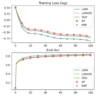
Figure 1: The results of LoRA and its simplifications. We apply the LoRA patch to the first layer of the network with a shape of $768\times 768$ and set $r=8$. The legend LoRA is the original LoRA method, while LoRA(B) is the simplification where only the matrix $B$ is updated. RP (random projection) and RRP (resampled RP) follow the same update rule (15), but RRP uses different projection matrices at different steps. In addition, we show the results of SGD on the full model for comparison. All experiments use the same $\eta=0.01$.

2.3 Our interpretation of LoRA

To this end, we provide a novel interpretation of a LoRA update by framing it as the compression and decompression of gradients.

Compression.

LoRA first compresses the gradient by a random down-projection, which can be justified by the following result based on the Johnson–Lindenstrauss lemma (Dasgupta and Gupta, 2003; Matoušek, 2008).

Lemma 2.3 (Indyk and Motwani).

Let $\epsilon\in(0,1/2]$ and $\delta\in(0,1)$. Let $A\in{\mathbb{R}}^{r\times m}$ be a random matrix where each element is independently sampled from a standard Gaussian distribution. There exists a constant $c$ such that when $r=c\epsilon^{-2}\log(\delta/2)$, we have

$$(1-\epsilon)\|x\|\leq(1/{\sqrt{r}})\|Ax\|\leq(1+\epsilon)\|x\|$$ (16)

with probability at least $1-\delta$ for every $x\in{\mathbb{R}}^{m}$.

Essentially, this lemma suggests that, with a high probability, the projection by a random Gaussian matrix largely preserves the scaled norm in the original space. In the case of LoRA, such a random projection is applied to each row of the gradient matrices, whose dimension is thus reduced from ${\mathbb{R}}^{n\times m}$ to ${\mathbb{R}}^{r\times m}$. The lemma asserts that the norm structure of the rows is approximately preserved.

Decompression.

After down-projection by $A_{0}^{\top}$, LoRA decomposes the gradient by an up-projection $A_{0}$. We show that this will recover the original gradient in expectation:

$$\mathop{\mathbb{E}}_{A_{0}}\left[W+(\nabla_{W}{\mathcal{L}}_{t})A_{0}^{\top}A_{0}\right]=W+(\nabla_{W}{\mathcal{L}}_{t})\mathop{\mathbb{E}}_{A_{0}}[A_{0}^{\top}A_{0}]$$ (17)

where $(1/r)\mathop{\mathbb{E}}_{A_{0}}[A_{0}^{\top}A_{0}]$ is an identity matrix. Moreover, the larger the rank $r$, the closer the expectation is to the identity. We quantify the error in our following theorem.

Theorem 2.4.

Let $A$ be a matrix of shape ${\mathbb{R}}^{r\times m}$ where each element is independently sampled from a standard Gaussian distribution. Let $\epsilon,\delta\in(0,1]$. There exists a constant $c$ such that when $r=c\log(2m/\delta)\epsilon^{-2}$, we have for all $i,j$ that

$$\Big{|}[A^{\top}A-I]_{i,j}\Big{|}\leq\epsilon$$ (18)

with confidence at least $1-\delta$.

Proof.

See Appendix B. ∎

Our Theorem 2.4 implies that $r$ only needs to scale logarithmically to preserve the element-wise reconstruction error, which is efficient in both computation and memory. Further, the logarithmic asymptotic rate makes it an ideal candidate to be applied to the training of modern neural models where $m$ is large.

We empirically verify our interpretation of LoRA by a pilot study on the Fashion-MNIST dataset (Xiao et al., 2017) with a simple feed-forward network. We experiment with a variant of LoRA where only $B$ is tuned; we call the variant LoRA(B). As shown in Figure 1, the performance of LoRA(B) is close to the original LoRA, which is consistent with Observation 2.2 and suggests the overall update of LoRA is dominated by the compression-and-decompression step. Further, the curve is identical to random projection (RP), well aligned with our derivation in Section 2.2.

2.4 Our method: Flora

Based on the analyses, we propose our method, Flora (from LoRA to high-rank updates), to enable overall high-rank updates. One of the main insights of Flora is that it constantly resamples the projection matrix in Equation (15). Therefore, our total weight change is no longer constrained to be low-rank. Moreover, we can apply the random-projection compression to the optimization states for memory saving. We demonstrate two common scenarios where Flora can be applied: (1) an arithmetic mean (AM) over a period of history, for which a concrete example is gradient accumulation; (2) an exponential moving average (EMA), for which an example could be momentum calculation. We show that compression of Flora has the same asymptotic rate as LoRA but with a lower constant.

Resampling random projection matrices.

With the approximation in Observation 2.2, LoRA can be viewed as having a fixed random projection matrix $A_{0}$. This restricts the overall change of $W$ to be low-rank. However, our analysis in Section 2.3 holds for any random matrix at every time step.

Therefore, we propose in Flora to resample a new random matrix to avoid the total change restricted in a low-rank subspace. In our pilot study, resampling the random matrix (RRP) largely recovers the performance of full-matrix SGD, significantly surpassing both the original LoRA and its approximated version in Equation (15). The empirical evidence highlights the effectiveness of avoiding the low-rank constraint in our Flora.

It should be emphasized that we cannot resample the down-projection matrix $A$ in LoRA. This is because $A$ and $B$ are coupled during the updates, and if the down-projection matrix $A$ is resampled, the already updated matrix $B$ will not fit. On the other hand, our Flora directly updates the weight matrix $W$ during training, making it flexible to choose a random down-projection at every step.

Algorithm 1 Gradient accumulation with Flora.

0:  rank $r\in{\mathbb{Z}}_{+}$

0:  accumulating steps $\tau\in{\mathbb{Z}}_{+}$

0:  gradient function $\nabla_{W}f(\cdot;\cdot)$

0:  weight matrices ${\mathbb{W}}=\left\{W^{(l)}:\dim(W^{(l)})=2\right\}$ $\rhd$ Initialization of the accumulator state

1:  for $W\in{\mathbb{W}}$ do

2:     $C_{W}\leftarrow\mathbf{0}^{n\times r}$ $\rhd$ $O(nr)$

3:     $s_{W}\leftarrow\text{an independent random seed}$

4:  end for$\rhd$ Accumulating the compressed gradients

5:  for $i\in[\tau]$ do

6:     for $W\in{\mathbb{W}}$ do

7:        $G_{W}\leftarrow\nabla_{W}f_{i}({\mathbb{W}})$ $\rhd$ $G_{W}\in{\mathbb{R}}^{n\times m}$

8:        $A_{W}\leftarrow{\mathcal{N}}_{s_{W}}(0,1/r)$ $\rhd$ $A_{W}\in{\mathbb{R}}^{r\times m}$

9:        $C_{W}\leftarrow C_{W}+G_{W}A_{W}^{\top}$ $\rhd$ Compresssion

10:     end for

11:  end for$\rhd$ Reconstruction

12:  for $W\in{\mathbb{W}}$ do

13:     $A_{W}\leftarrow{\mathcal{N}}_{s_{W}}(0,1/r)$ $\rhd$ $A_{W}\in{\mathbb{R}}^{r\times m}$

14:     $\tilde{G}_{W}\leftarrow(1/n)D_{W}A_{W}$ $\rhd$ Decompression

15:  end for

16:  return $\{\tilde{G}_{W}:W\in{\mathbb{W}}\}$ $\rhd$ Overwrite $\{G_{W}\}$

Algorithm 2 Momentum with Flora.

0:  decay rates $0\leq\beta\leq 1$

0:  rank $r\in{\mathbb{Z}}_{+}$, interval $\kappa\in{\mathbb{Z}}_{+}$

0:  gradient function $\nabla_{W}f(\cdot;\cdot)$

0:  weight ${\mathbb{W}}=\left\{W^{(l)}:\dim(W^{(l)})=2\right\}$ $\rhd$ Initialize the optimizer state

1:  $t\leftarrow 0$

2:  for $W\in{\mathbb{W}}$ do

3:     $M_{t,W}\leftarrow\mathbf{0}^{n\times r}$

4:     $s_{t,W}\leftarrow\text{an independent random seed}$

5:  end for$\rhd$ Training procedure

6:  while training not converged do

7:     for $W\in{\mathbb{W}}$ do

8:        $G_{t,W}\leftarrow\nabla_{W}f_{t}({\mathbb{W}})$ $\rhd$ $G_{t,W}\in{\mathbb{R}}^{n\times m}$

9:        $A_{t,W}\sim{\mathcal{N}}_{s_{t,W}}(0,1/r)$ $\rhd$ $A_{t,W}\in{\mathbb{R}}^{r\times m}$

10:        if $t\equiv 0\pmod{\kappa}$ then

11:           $s_{t+1,W}\leftarrow\text{an independent random seed}$

12:           $A^{\prime}_{W}\sim{\mathcal{N}}_{s_{t+1,W}}(0,1/r)$ $\rhd$ $A^{\prime}_{W}\in{\mathbb{R}}^{r\times m}$

13:           $M^{\prime}\leftarrow M_{t,W}A_{t,W}A_{t+1,W}^{\top}$

14:        else

15:           $s_{t+1,W}\leftarrow s_{t,W}$

16:           $A^{\prime}_{W}\leftarrow A_{t,W}$

17:           $M^{\prime}\leftarrow M_{t,W}$

18:        end if

19:        $M_{t+1,W}\leftarrow\beta M^{\prime}+(1-\beta)G_{t,W}{A^{\prime}_{W}}^{\top}$

20:     end for

21:     yield $\{M_{t+1,W}A^{\prime}_{W}:W\in{\mathbb{W}}\}$ $\rhd$ Decompression

22:     $t\leftarrow t+1$

23:  end while

Sublinear memory gradient accumulation.

One application of our Flora is to compress the optimization states to save memory during training. We first show this with an example of gradient accumulation, which is widely used in practice to simulate a larger batch size (Smith et al., 2018). Specifically, it calculates the arithmetic mean (AM) of gradients for $\tau$ steps and updates the model by the AM. In this way, the effective batch size is $\tau$ times larger than the original batch size. However, it requires a memory buffer, whose size is equal to the model itself, to store the accumulated gradients.

In Flora, we propose to compress the gradient accumulation with the down-projection. Within an accumulation cycle, we only maintain the accumulated gradient in the randomly down-projected space. During decompression, we can reuse the memory for gradients to reduce additional overheads. The resampling of the projection matrix occurs when an accumulation cycle is finished. The overall algorithm is summarized in Algorithm 1.

Sublinear memory momentum.

The momentum technique is widely used in modern deep learning to reduce the variance of the gradient and accelerate training (Nesterov, 1998; Goh, 2017; Jelassi and Li, 2022). However, it requires maintaining an additional momentum scalar for each parameter, which is expensive when the model is large.

Similar to the compressed gradient accumulation, we can also compress the momentum with Flora. For each time step $t$, we down-project the new gradient $G_{t}$ by a random projection matrix $A_{t}^{\top}$. However, the difficulty for accumulating momentum emerges when we use a $A_{t}$ different from $A_{t-1}$, as we cannot reconstruct the original momentum from $G_{t-1}A^{\top}_{t-1}+G_{t}A_{t}^{\top}$. This difficulty applies to all EMA updates where the number of accumulation steps is not finite. In this case, resampling new matrices will result in a loss of historical accumulation.

We propose two remedies to address this issue. First, we keep the same projection matrix for a long time to reduce the distortion. Second, we propose to transfer the compressed momentum from the old projection to a new one by $M_{t}=M_{t-1}A_{t-1}A_{t}^{\top}$. This is justified by $A_{t-1}^{\top}A_{t-1}$ and $A_{t}^{\top}A_{t}$ are approximately the identity matrix based on Theorem 2.4.

The final algorithm is shown in Algorithm 2. Overall, for each weight matrix $W\in\mathbb{R}^{n\times m}$, we preserve the momentum term $M_{t}$ with sublinear memory. Compared with the original momentum, we reduce the memory from $O(nm)$ to $O(nr)$. It should be pointed out that although we track momentum specifically in this case, our algorithm can be easily extended to other EMA-based statistics.

Table 1: The results of different methods to compress gradient accumulation. The size indicates the total number of the original model parameters. The numbers in the brackets denote the rank $r$ of the random projection matrix.

(a) The results of T5 variants on XSum.

Size	Accumulation	Mem	$\Delta_{M}$	R1/R2/R${}_{\text{L}}$
60M	None	0.75	-	33.4/11.4/26.4
	Naive	0.87	0.12	34.0/11.5/26.7
	LoRA(8)	0.82	0.07	30.4/8.60/23.6
	LoRA(32)	0.86	0.11	30.7/8.90/23.9
	LoRA(128)	0.94	0.19	31.0/9.10/24.1
	LoRA(256)	1.07	0.32	31.4/9.34/24.5
	Flora(8)	0.75	0.00	31.5/9.67/24.6
	Flora(32)	0.75	0.00	32.2/10.3/25.2
	Flora(128)	0.77	0.02	33.2/10.9/26.0
	Flora(256)	0.79	0.04	33.6/11.3/26.5
3B	None	16.7	-	42.5/19.1/34.6
	Naive	26.6	9.9	44.4/20.9/36.3
	LoRA(16)	27.8	11.1	42.2/18.4/34.0
	LoRA(64)	29.5	12.8	42.3/18.6/34.1
	LoRA(256)	33.4	16.7	42.6/18.9/34.4
	LoRA(512)	OOM	-	-
	Flora(16)	17.0	0.3	43.5/20.0/35.5
	Flora (64)	18.2	1.5	43.9/20.3/35.8
	Flora (256)	19.5	2.8	44.3/20.7/36.2
	Flora (512)	22.1	5.4	44.5/20.9/36.4

(b) The results of GPT-2 variants on IWSLT17 De-En.

Size	Accumulation	Mem	$\Delta_{M}$	BLEU
110M	None	2.77	-	17.9
	Naive	3.24	0.47	24.9
	LoRA(8)	3.25	0.48	9.94
	LoRA(32)	3.29	0.52	11.2
	LoRA(128)	3.38	0.60	12.2
	LoRA(256)	3.52	0.75	13.4
	Flora (8)	2.93	0.15	16.3
	Flora (32)	2.94	0.16	22.0
	Flora (128)	2.98	0.20	24.0
	Flora (256)	3.03	0.26	25.4
1.5B	None	20.8	-	28.2
	Naive	26.5	5.78	33.2
	LoRA(16)	26.8	6.02	17.4
	LoRA(64)	27.4	6.68	19.5
	LoRA(256)	28.9	8.15	20.7
	LoRA(512)	OOM	-	-
	Flora (16)	21.1	0.34	29.7
	Flora (64)	21.3	0.52	31.6
	Flora (256)	21.9	1.17	33.2
	Flora (512)	22.8	2.04	33.6

Memory analysis.

It should be pointed out that neither LoRA nor our Flora saves the memory for back-propagation. This is because $\tfrac{\partial{\mathcal{L}}}{\partial W}$ is needed for the update of $A$ and $B$ in LoRA (Dettmers et al., 2023), while in our approach we also compress and decompress the gradient.

That being said, saving the memory of optimization states alone could be critical to training large models (Dettmers et al., 2021). Our Flora compresses both the AM and EMA of gradients to the sublinear level, which shares the same asymptotic rate as LoRA. In implementation, we may store the random seed that generates the projection matrix—which is highly efficient, as each element can be sampled independently with simple operations—instead of maintaining the same project matrix over batches. This allows the program to further save memory in practice with buffer reuse. On the contrary, LoRA needs to maintain two weight matrices $A$ and $B$, as well as their AM or EMA matrices. Empirically shown in Section 3, Flora consumes less memory than LoRA while facilitating high-rank updates and outperforming LoRA to a large extent.

3 Experiments

In this section, we empirically verify the effectiveness of our approach across different model architectures and datasets.

3.1 Experiment setup

Models.

Given the exceptional ability of language models, we consider Transformer-based models for our experiments. Specifically, we select two representative models, including the T5 (Raffel et al., 2020) and GPT-2 (Radford et al., 2019) series. For the T5 series, we use T5-small to represent small models and T5-3B to represent large models. T5-small has around 60M parameters, with a hidden dimension set to 512, while T5-3B has around 3B parameters with a hidden dimension of 1024. For the GPT-2 series, we use the base version to represent small models and GPT-2-XL to represent large models. The base version has around 110M parameters, with a hidden dimension set to 768, while the large version has around 1.5B parameters with a hidden dimension of 1600.

Datasets.

To facilitate evaluation, we use two conditional language modeling tasks, including summarization and translation.

For the summarization task, we train T5 on the XSum dataset (Narayan et al., 2018). Each sample is a news article with a summary. The task is to generate a summary of the article. For each input, we prepend the prefix “summarize:” to the source sentence in the encoder (Raffel et al., 2020). The source and target sentences are truncated to 512 and 128 tokens, respectively.

For the translation task, we follow the setting of Lin et al. (2020) and train GPT-2 on the IWSLT-2017 German-English dataset (Cettolo et al., 2017). Each sample is a German sentence with its English translation. The task is to generate the English translation of the German sentence. For each input, we use the template “translate German to English: [source]. English: [target]” for training (Raffel et al., 2020).

Evaluation metrics.

For the summarization task, we use the widely used ROUGE scores (Lin, 2004), including ROUGE-1, ROUGE-2, and ROUGE-L (R₁/R₂/R${}_{\text{L}}$) to evaluate the quality of the generated summary. For the translation task, we use the most commonly used SacreBLEU score (Post, 2018) to evaluate the translation quality. For both ROUGE and SacreBLEU scores, the higher the score, the better the quality of the generated text.

To get more insights into the training process, we monitor the peak memory usage with the built-in JAX profiling tool (Bradbury et al., 2018). We also show the excessive memory $\Delta_{M}$ compared with the method where accumulation or momentum is disabled. The memory is reported in GiB ($1024^{3}$ bytes).

Competing methods.

In our experiment, we take Adafactor as the base optimizer, which is the default optimizer for many Transformer models including T5 (Raffel et al., 2020), and is reported to be empirically better than Adam (Rae et al., 2021). We use the official Adafactor implementation in Optax (DeepMind et al., 2020).

We compare the following methods: (1) None: a baseline that does not use gradient accumulation or momentum; (2) Naive: a naive implementation of gradient accumulation or momentum, which stores the full information along training; (3) LoRA: the original LoRA method where only the LoRA patches are trained; (4) Flora: our approach that compresses the gradients and decompresses them when updating the original weights. For LoRA and Flora, we apply the projections to attention and feed-forward layers only, while following the naive procedure for other layers (i.e., token embeddings and vector weights).

For small models (T5-small and GPT-2 base), we test the rank $r$ from 8 to 256, ranging from the very low dimension to half of the hidden dimension, for a thorough examination of different methods. For large models (T5-3B and GPT-2-XL), we test $r$ from 16 to 512 to approximately maintain the same percentage of memory saving as small models. We do not apply learning rate schedules (Loshchilov and Hutter, 2017) or weight decay (Loshchilov and Hutter, 2019) in any experiments to rule out the influence of these techniques.

3.2 Main results

Gradient accumulation.

In this setting, we fine-tune pre-trained models with 16 gradient accumulation steps. To achieve a minimal memory footprint and fit large models, the physical batch size is set to 1. We sweep the learning rate from $10^{-5}$ to $10^{-1}$ with the naive accumulation method on the validation loss. The best learning rate is applied to other methods excluding LoRA, which is tuned individually as it is reported to have different optimal learning rates (Hu et al., 2022). For each run, the model is fine-tuned for 1 epoch to prevent over-fitting following the common practice (Wu et al., 2021). The results are reported on the test set based on the checkpoint with the lowest validation loss.

We present the results in Table 1. As shown, the naive gradient accumulation improves the ROUGE scores over the method without accumulation, but it leads to a large memory usage, which is similar to the model size, to store the accumulation. For LoRA, we empirically observe that it generally does not reduce memory usage in this case as the state of Adafactor is already sublinear. In fact, it increases memory because it stores another four low-rank matrices for each weight matrix and adds an additional Jacobian path for the automatic differentiation.

On the contrary, our Flora reduces the memory footprint on all benchmarks compared with the naive accumulation. In addition, when $r$ is reasonably large, our method is able to recover the performance (in ROUGE or BLEU scores) of full-matrix accumulation and surpass the baseline that accumulation is not enabled. Notably, for the large models (T5-3B and GPT-2-XL), the memory overhead of Flora ($r=256$) is only $30\%$ of the naive accumulation, while the performance is on par.

Table 2: The results of compressing momentum. The size indicates the total number of the original model parameters. The numbers in the brackets denote the rank $r$ of the random projection matrix.

Setting	Momentum	Mem	R1/R2/R${}_{\text{L}}$
T5 60M XSum	None	1.65	29.4/9.11/23.3
	Naive	1.89	29.9/9.40/23.8
	LoRA(8)	1.88	18.0/3.33/14.9
	LoRA(32)	1.91	20.4/4.20/16.7/
	LoRA(128)	2.05	21.5/4.82/17.4
	LoRA(256)	2.13	22.2/5.04/17.9
	Flora(8)	1.71	25.5/6.56/20.4
	Flora (32)	1.72	26.9/7.32/21.5
	Flora (128)	1.75	29.1/8.76/23.2
	Flora (256)	1.79	30.2/9.51/24.0

Setting	Momentum	Mem	BLEU
GPT-2 110M IWSLT17	None	8.95	19.4
	Naive	9.45	19.9
	LoRA(8)	9.42	4.98
	LoRA(32)	9.46	6.76
	LoRA(128)	9.55	8.72
	LoRA(256)	9.76	9.83
	Flora (8)	9.09	9.14
	Flora (32)	9.10	14.9
	Flora (128)	9.14	18.6
	Flora (256)	9.20	19.9

Momentum.

Given that the momentum technique is ineffective in fine-tuning (Li et al., 2020), we train all models from scratch in this setting. The physical batch size is set to $4$ as a result of balancing the generalization and variance reduction (Masters and Luschi, 2018). We disable the gradient accumulation technique to rule out its impact. Due to the expense of training from scratch, we only test the small variants of each series. Similar to the settings in gradient accumulation, we sweep the learning rate for the naive momentum method from $10^{-5}$ to $10^{-1}$ on the validation loss. The best learning rates are applied to all methods excluding LoRA, which again has its own optimal learning rate. The hyper-parameter $\kappa$ (resampling interval) is set to $1000$ for all runs of Flora. The effect of different values of $\kappa$ is shown in Section 3.3.

As shown in Table 2, the naive momentum technique achieves better performance than at a cost of more memory usage. Similar to the results in gradient accumulation, LoRA does not save memory given the optimization state is already sublinear. It also has a significantly lower performance when trained from scratch, as the overall matrix update can only be low-rank.

Our Flora utilizes less memory than the naive momentum. In addition, our method recovers (or even surpasses) the performance of naive momentum when $r$ is increased. This significantly distinguishes our methods from LoRA as it achieves memory-efficient training even when the initialization is random.

3.3 In-depth analyses

The effect of $\kappa$ in momentum.

In our momentum implementation, we have a hyper-parameter $\kappa$ controlling the resampling frequency of the random-projection matrix. In this part, we analyze the effect of $\kappa$ with T5-small on the summarization task as our testbed, due to the limit of time and resources. We vary $\kappa$ by keeping other hyper-parameters the same as in Section 3.2.

The results are shown in Table 3. It is seen that, when $\kappa$ is below $1000$, the ROUGE scores increase with $\kappa$. After a certain threshold, however, we see that the performance starts to decrease. This aligns with our interpretation that the information is better preserved within the interval, but each interval is bottlenecked by the rank. Given the results, we choose $\kappa=1000$ in Section 3.2 to balance the preserved information and the overall rank of momentum.

Optimizer with linear memory.

In our main experiments, we observed a counter-intuitive phenomenon that LoRA empirically increases memory usage. This is likely because that the optimization states in Adafactor are already sublinear, rendering the ineffectiveness of LoRA to save memory in this case. To further verify our method in linear-memory optimizers, we test the performance with a variant of Adafactor where the second-moment estimates are not factorized, essentially making it a linear-memory optimizer. All the other hyper-parameters remain the same as Section 3.2.

Table 4 shows the results. As seen, LoRA indeed saves more memory than our Flora when the rank is low ($r<$128) in linear-memory optimizers. However, our Flora becomes more memory-efficient for $r=256$, because we have a lower constant in the complexity. Moreover, our Flora largely outperforms LoRA in all settings by 2–3 ROUGE points, showing the superiority of our approach.

Table 3: The effect of $\kappa$ in momentum.

Setting	$\kappa$	Mem	R1/R2/R${}_{\text{L}}$
T5 60M XSum	1	1.79	0.00/0.00/0.00
	10	1.79	27.5/7.68/31.8
	100	1.79	29.3/8.89/23.2
	1000	1.79	30.4/9.70/24.2
	10000	1.79	29.5/9.11/23.5

Table 4: The results of linear-memory optimizers.

Setting	Accumulation	Mem	R1/R2/R${}_{\text{L}}$
T5 60M XSum	None	0.99	33.0/11.1/26.1
	Naive	1.12	34.0/11.5/26.7
	LoRA(8)	0.82	28.7/7.51/22.0
	LoRA(32)	0.86	29.0/7.71/22.3
	LoRA(128)	1.00	29.7/8.02/22.9
	LoRA(256)	1.20	30.0/8.28/23.2
	Flora (8)	1.00	31.6/9.72/24.7
	Flora (32)	1.00	32.3/10.3/25.3
	Flora (128)	1.00	33.2/10.9/26.0
	Flora (256)	1.04	33.5/11.1/26.3

4 Related work and discussion

Parameter efficient fine-tuning.

Many methods have been proposed to improve the parameter efficiency of fine-tuning large models. A straightforward way is to tune a subset of the model, such as the top layers (Li and Liang, 2021) and bias vectors (Zaken et al., 2022). Another way is to add small tunable modules (e.g., Adapter Houlsby et al., 2019 and LoRA Hu et al., 2022) to the pre-trained model. Although reducing the optimization memory, these methods suffer from the problem that the model parameters are restricted. For example, the total weight change of LoRA is constrained to be low-rank. In an attempt to achieve high-rank updates, ReLoRA (Lialin et al., 2023) proposes to periodically reinitialize the LoRA patch. However, it requires full-weight pre-training to work properly, growing the peak memory linearly in model size. We hence do not include ReLoRA as a sublinear-memory baseline. By contrast, our method is able to directly start from scratch and achieve the full-training performance, while maintaining a sublinear complexity throughout the process.

Matrix compression.

Our method is closely connected to matrix compression techniques. For example, principal component analysis (Shlens, 2014) or matrix sketching (Liberty, 2013) use singular value decomposition (SVD) to approximate the large matrix with smaller matrices. However, the SVD procedure is computationally expensive and difficult to be parallelized, making it impractical for large-scale training. Another way to compress the matrix is to use random projection (Bingham and Mannila, 2001), which lies the foundation of our method. Our method additionally involves a simple and efficient decompression procedure justified by Theorem 2.4. The simplification saves both computation and memory usage.

Memory-efficient optimizers.

Optimization states contribute significantly to memory usage for large-scale training (Dettmers et al., 2021). Memory-efficient optimizers (Shazeer and Stern, 2018; Feinberg et al., 2023) are shown to effectively reduce the memory footprint. Our method is orthogonal to these methods, as it can be applied to enhance existing optimizers by compressing the momentum or gradient accumulation.

Memory-efficient automatic differentiation.

It is also possible to reduce the memory footprint of back-propagation with advanced techniques like gradient checkpointing (Chen et al., 2016), mixed-precision training (Micikevicius et al., 2018), randomized auto differentiation (Oktay et al., 2020), or zeroth-order optimization (Malladi et al., 2023). Technically, Flora can be combined with these methods to further save memory. We leave it to future work given our focus in this paper is to compress optimization states.

5 Conclusion

Summary.

In this work, we introduce Flora, a method based on random projections that achieves sublinear memory usage for gradient accumulation and momentum. In addition, our approach effectively addresses the low-rank limitation of LoRA by resampling projection matrices. Experimental results demonstrate significant memory reduction with maintained model performance, highlighting the potential of random projection in deep learning.

Future work.

In this paper, the largest model is 3B. For extremely large models like GPT-3, we estimate that the compressed optimization state of $r=256$ is only 2.08% of its original memory, which would be of great practical significance. We leave the empirical verification to future work. Further, the applicable scope of Flora is not limited to language models. We would like to test it in more cases.

Appendix A Proof of Theorem 2.1

See 2.1

Before proving the theorem, we need to obtain the form of $f_{A}(t)$ and $f_{B}(t)$. We derive them in the following lemma.

Lemma A.1.

When $t=0$, $f_{A}(0)=f_{B}(0)=0$. For $t\geq 1$, the values of $f_{A}(t)$ and $f_{B}(t)$ are iteratively obtained by:

$$f_{A}(t) =-\eta\sum_{i=0}^{t-1}f_{B}^{\top}(i)(\nabla_{W}{\mathcal{L}}_{i})$$ (19)

$$f_{B}(t) =-\sum_{i=0}^{t-1}(\nabla_{W}{\mathcal{L}}_{i})(\eta f_{A}^{\top}(i)+I)$$ (20)

Proof.

We prove this by induction. For the base case $t=0$, it is straightforward to show $f_{A}(0)=f_{B}(0)=0$.

Assume $A_{t}=A_{0}+\eta A_{0}f_{A}(t)$ and $B_{t}=\eta f_{B}(t)A_{0}^{\top}$ holds with such functions $f_{A}$ and $f_{B}$ for $1\dots t$. Then for $t+1$, we have

$$A_{t+1}= A_{t}-\eta B_{t}^{\top}(\nabla_{W}{\mathcal{L}}_{t})$$ (21)

$$= A_{0}+\eta A_{0}f_{A}(t)-\eta^{2}A_{0}f_{B}^{\top}(t)(\nabla_{W}{\mathcal{L}}_{t})$$ (22)

$$= A_{0}+\eta A_{0}\left(f_{A}(t)-\eta f_{B}^{\top}(t)(\nabla_{W}{\mathcal{L}}_{t})\right)$$ (23)

$$= A_{0}+\eta A_{0}\left(f_{A}(t+1)\right),$$ (24)

where we have $f_{A}(t+1)=f_{A}(t)-\eta f_{B}^{\top}(t)(\nabla_{W}{\mathcal{L}}_{t})=-\eta\sum_{i=0}^{t}f_{B}^{\top}(i)(\nabla_{W}{\mathcal{L}}_{i})$ in the last line.

Similarly, we have

$$B_{t+1}= B_{t}-\eta(\nabla_{W}{\mathcal{L}}_{t})A_{t}^{\top}$$ (25)

$$= \eta f_{B}(t)A_{0}^{\top}-\eta(\nabla_{W}{\mathcal{L}}_{t})(\eta f_{A}^{\top}(t)+I)A_{0}^{\top}$$ (26)

$$= \eta\left(f_{B}(t)-(\nabla_{W}{\mathcal{L}}_{t})(\eta f_{A}^{\top}(t)+I)\right)A_{0}^{\top}$$ (27)

$$= \eta f_{B}(t+1)A_{0}^{\top},$$ (28)

where we have $f_{B}(t+1)=f_{B}(t)-(\nabla_{W}{\mathcal{L}}_{t})(\eta f_{A}^{\top}(t)+I)=-\sum_{i=0}^{t}(\nabla_{W}{\mathcal{L}}_{i})(\eta f_{A}^{\top}(i)+I)$ in the last line. ∎

Proof of Theorem 2.1.

Define $a_{t}:=\frac{\eta L^{2}\big{(}1-(\eta^{2}L^{2})^{t}\big{)}}{1-\eta^{2}L^{2}}.$ We prove $\|f_{A}(t)\|\leq a_{t}$ by induction. For the base case $t=0$, it is trivial to see $\|f_{A}(0)\|=0\leq a_{0}$. We then assume $\|f_{A}(i)\|\leq a_{i}$ for $i\leq t-1$. Since $a_{t}$ is monotonically increasing, we know $\|f_{A}(i)\|\leq a_{t-1}$ for $i\leq t-1$. By using Lemma A.1, we have

$$f_{A}(t)= -\eta\sum_{i=0}^{t-1}f_{B}^{\top}(i)(\nabla_{W}{\mathcal{L}}_{i})$$ (29)

$$= -\eta\sum_{i=1}^{t-1}\sum_{j=0}^{i-1}(\eta f_{A}(j)+I)(\nabla_{W}{\mathcal{L}}_{j})^{\top}(\nabla_{W}{\mathcal{L}}_{i}).$$ (30)

Taking the norm, we have

$$\|f_{A}(t)\|_{F}= \left\|\eta\sum_{i=1}^{t-1}\sum_{j=0}^{i-1}(\eta f_{A}(j)+I)(\nabla_{W}{\mathcal{L}}_{j})^{\top}(\nabla_{W}{\mathcal{L}}_{i})\right\|_{F}$$ (31)

$$\leq \eta^{2}\left\|\sum_{j=0}^{t-2}(f_{A}(j))(\nabla_{W}{\mathcal{L}}_{j})^{\top}\sum_{i=j+1}^{t-1}(\nabla_{W}{\mathcal{L}}_{i})\right\|_{F}+\eta\left\|\sum_{i=1}^{t-1}\sum_{j=0}^{i-1}(\nabla_{W}{\mathcal{L}}_{j})^{\top}(\nabla_{W}{\mathcal{L}}_{i})\right\|_{F}$$ (32)

$$\leq \eta^{2}L\left\|\sum_{j=0}^{t-2}(f_{A}(j))(\nabla_{W}{\mathcal{L}}_{j})^{\top}\right\|_{F}+\eta L^{2}$$ (Lemma A.2)

$$\leq \eta^{2}L^{2}a_{t-1}+\eta L^{2}$$ (Lemma A.3)

$$= \eta^{2}L^{2}\frac{\eta L^{2}-(\eta^{2}L^{2})^{t}}{1-\eta^{2}L^{2}}+\eta L^{2}$$ (33)

$$= \frac{\eta L^{2}-(\eta^{2}L^{2})^{t+1}}{1-\eta^{2}L^{2}}$$ (34)

$$= a_{t}.$$ (35)

Therefore, we have $\|f_{A}(t)\|\leq\|f_{A}(t)\|_{F}\leq a_{t}$ for every $t$. ∎

Lemma A.2.

If $\|\sum_{k=0}^{t-1}(\nabla_{W}{\mathcal{L}}_{j})^{\top}\|_{F}\leq L$, we have

$$\left\|\sum_{i=1}^{t-1}\sum_{j=0}^{i-1}(\nabla_{W}{\mathcal{L}}_{j})^{\top}(\nabla_{W}{\mathcal{L}}_{i})\right\|_{F}\leq L^{2}$$ (36)

for every $t$.

Proof.

Let $G(k):=\nabla_{W}{\mathcal{L}}_{k}$ for simplicity. Taking the square,

$$\left\|\sum_{n}\sum_{m=1}^{n}G(m)^{\top}G(n)\right\|_{F}^{2}= \sum_{i,j}\sum_{n}\sum_{m=1}^{n}[G(m)^{\top}G(n)]_{i,j}^{2}$$ (37)

$$= \sum_{i,j}\sum_{n}\sum_{m=1}^{n}\Big{(}\sum_{k}[G(m)]_{k,i}[G(n)]_{k,j}\Big{)}^{2}$$ (38)

$$\leq \Big{(}\sum_{m}\sum_{i}\sum_{k}[G(m)]_{k,i}^{2}\Big{)}\Big{(}\sum_{m=n}^{t-1}\sum_{j}\sum_{k}[G(n)]_{k,j}^{2}\Big{)}$$ (Cauchy-Schwarz)

$$\leq \bigg{(}\sum_{m}\sum_{i}\sum_{k}[G(m)]_{k,i}^{2}\bigg{)}^{2}$$ (39)

$$\leq \bigg{(}\sum_{i}\sum_{k}\Big{(}\sum_{m}[G(m)]_{k,i}\Big{)}^{2}\bigg{)}^{2}$$ (40)

$$= \Big{\|}\sum_{m}G(m)\Big{\|}_{F}^{4}$$ (41)

$$\leq L^{4},$$ (42)

which completes the proof by taking square roots on both sides. ∎

Lemma A.3.

If $\|f_{A}(k)\|_{F}\leq a_{k}$ for all $k<t$, we have

$$\left\|\sum_{k=0}^{t-1}f_{A}(k)(\nabla_{W}{\mathcal{L}}_{k})^{\top}\right\|_{F}\leq a_{t-1}L$$ (43)

for every $t$.

Proof.

Let $A(k):=f_{A}(k)$ and $G(k)=(\nabla_{W}{\mathcal{L}}_{k})$ for simplicity. Taking the square,

$$\Big{\|}\sum_{k=0}^{t-1}A(k)G(k)^{\top}\Big{\|}_{F}^{2}= \sum_{k=0}^{t-1}\sum_{i}\sum_{j}[A(k)G(k)^{\top}]^{2}_{i,j}$$ (44)

$$= \sum_{k=0}^{t-1}\sum_{i}\sum_{j}\Big{(}\sum_{l}[A(k)]_{i,l}[G(k)]_{j,l}\Big{)}^{2}$$ (45)

$$= \sum_{k=0}^{t-1}\Big{(}\sum_{i}\sum_{l}[A(k)]_{i,l}^{2}\Big{)}\Big{(}\sum_{j}\sum_{l}[G(k)]_{j,l}^{2}\Big{)}$$ ( Cauchy–Schwarz)

$$\leq \Big{(}\max_{0\leq k<t}\sum_{i}\sum_{l}[A(k)]_{i,l}^{2}\Big{)}\sum_{k=0}^{t-1}\Big{(}\sum_{j}\sum_{l}[G(k)]_{j,l}^{2}\Big{)}$$ (46)

$$\leq \Big{(}\max_{0\leq k<t}\sum_{i}\sum_{l}[A(k)_{i,l}]^{2}\Big{)}\Big{(}\sum_{j}\sum_{l}(\sum_{k=0}^{t-1}[G(k)]_{j,l})^{2}\Big{)}$$ (47)

$$= \Big{(}\max_{0\leq k<t}\|A(k)\|_{F}^{2}\Big{)}\Big{\|}\sum_{k=0}^{t-1}G(k)\Big{\|}_{F}^{2}$$ (48)

$$\leq a_{t-1}^{2}L^{2},$$ (49)

which completes the proof by taking square roots on both sides. ∎

Appendix B Proof of Theorem 2.4

See 2.4

Proof.

For each element of $A^{\top}A$, we have

$$[A^{\top}A]_{i,j}=\begin{cases}\sum_{k=1}^{r}a_{k,i}^{2},&\text{ if }i=j,\\ \sum_{k=1}^{r}a_{k,i}a_{k,j},&\text{ otherwise, }\end{cases}$$ (50)

where each element $a_{i,k}$ is an independent random variable following ${\mathcal{N}}(0,1)$.

For $z_{i,i}:=\sum_{k=1}^{r}a_{k,i}^{2}$, it follows the $\chi^{2}(r)$ distribution. By the standard Laurent-Massart bounds Laurent and Massart (2000), we obtain

$$\delta_{i,i}:=\Big{|}\frac{z_{i,i}}{r}-1\Big{|}\leq 2\sqrt{\frac{\log(2/\delta_{1}^{\prime})}{r}}+2\frac{\log(2/\delta_{1}^{\prime})}{r}$$ (51)

with probability at least $1-\delta_{1}^{\prime}$.

For $z_{i,j}:=\sum_{k=1}^{r}a_{k,i}a_{k,j}$ where $i\not=j$, we can rewrite it as $z_{i,j}=\sum_{k=1}^{r}[(\frac{a_{k,i}+a_{k,j}}{2})^{2}-(\frac{a_{k,i}-a_{k,j}}{2})^{2}]$. In addition, all $(\frac{a_{k,i}+a_{k,j}}{2})^{2}$ and $(\frac{a_{k,i}-a_{k,j}}{2})^{2}$ are i.i.d. $\chi^{2}(1)$ distributions. Define

$$z^{+}_{i,j}:=\sum_{k=1}^{r}\bigg{(}\frac{a_{k,i}+a_{k,j}}{2}\bigg{)}^{2}\quad\text{and}\quad z^{-}_{i,j}:=\sum_{k=1}^{r}\bigg{(}\frac{a_{k,i}-a_{k,j}}{2}\bigg{)}^{2},$$ (52)

it is easy to see that $z^{+}_{i,j}$ and $z^{-}_{i,j}$ are i.i.d. $\chi^{2}(r)$ distributions. In addition, $z_{i,j}=z^{+}_{i,j}-z^{-}_{i,j}$. Therefore, we have

$$\delta_{i,j}:= \Big{|}\frac{z_{i,j}}{r}\Big{|}=\bigg{|}\Big{(}\frac{z_{i,j}^{+}}{r}-1\Big{)}-\Big{(}\frac{z_{i,j}^{-}}{r}-1\Big{)}\bigg{|}$$ (53)

$$\leq \Big{|}\frac{z_{i,j}^{+}}{r}-1\Big{|}+\Big{|}\frac{z_{i,j}^{-}}{r}-1\Big{|}$$ (54)

$$\leq 4\sqrt{\frac{\log(4/\delta_{2}^{\prime})}{r}}+4\frac{\log(4/\delta_{2}^{\prime})}{r}$$ (55)

with probability at least $1-\delta_{2}^{\prime}$.

By using a union bound upon Equation (51) and (55), we can obtain

$$\delta_{i,j}\leq 4\sqrt{\frac{2\log(2m/\delta)}{r}}+4\frac{2\log(2m/\delta)}{r}$$ (56)

for all $i,j$ with probability at least $1-\delta$. Under this condition, we further have

$$\delta_{i,j}= 4\sqrt{\frac{2\log(2m/\delta)}{128\log(2m/\delta)\epsilon^{-2}}}+4\frac{2\log(2m/\delta)}{128\log(2m/\delta)\epsilon^{-2}} r=128\log(2m/\delta)\epsilon^{-2}$$ (Let )

$$= \frac{1}{2}(\epsilon+\epsilon^{2})$$ (57)

$$\leq \epsilon, \epsilon^{2}\leq\epsilon\leq 1$$ ()

concluding the proof by noticing $\delta_{i,j}=\Big{|}[A^{\top}A-I]_{i,j}\Big{|}$. ∎

References

- Duchi et al. (2011) John Duchi, Elad Hazan, and Yoram Singer. Adaptive subgradient methods for online learning and stochastic optimization. JMLR, 12(7), 2011. URL https://jmlr.org/papers/v12/duchi11a.html.
- Hinton et al. (2012) Geoffrey Hinton, Nitish Srivastava, and Kevin Swersky. Neural networks for machine learning lecture 6a overview of mini-batch gradient descent. Coursera, 2012. URL https://www.cs.toronto.edu/~tijmen/csc321/slides/lecture_slides_lec6.pdf.
- Cutkosky and Orabona (2019) Ashok Cutkosky and Francesco Orabona. Momentum-based variance reduction in non-convex SGD. In NeurIPS, 2019. URL https://papers.nips.cc/paper_files/paper/2019/hash/b8002139cdde66b87638f7f91d169d96-Abstract.html.
- Goh (2017) Gabriel Goh. Why momentum really works. Distill, 2017. URL http://distill.pub/2017/momentum.
- Wang et al. (2013) Chong Wang, Xi Chen, Alexander J Smola, and Eric P Xing. Variance reduction for stochastic gradient optimization. In NIPS, 2013. URL https://papers.nips.cc/paper_files/paper/2013/hash/9766527f2b5d3e95d4a733fcfb77bd7e-Abstract.html.
- Brown et al. (2020) Tom Brown, Benjamin Mann, Nick Ryder, Melanie Subbiah, Jared D Kaplan, Prafulla Dhariwal, Arvind Neelakantan, Pranav Shyam, Girish Sastry, Amanda Askell, Sandhini Agarwal, Ariel Herbert-Voss, Gretchen Krueger, Tom Henighan, Rewon Child, Aditya Ramesh, Daniel Ziegler, Jeffrey Wu, Clemens Winter, Chris Hesse, Mark Chen, Eric Sigler, Mateusz Litwin, Scott Gray, Benjamin Chess, Jack Clark, Christopher Berner, Sam McCandlish, Alec Radford, Ilya Sutskever, and Dario Amodei. Language models are few-shot learners. In NeurIPS, pages 1877–1901, 2020. URL https://papers.nips.cc/paper/2020/hash/1457c0d6bfcb4967418bfb8ac142f64a-Abstract.html.
- Rombach et al. (2022) Robin Rombach, Andreas Blattmann, Dominik Lorenz, Patrick Esser, and Björn Ommer. High-resolution image synthesis with latent diffusion models. In CVPR, pages 10684–10695, 2022. URL https://openaccess.thecvf.com/content/CVPR2022/html/Rombach_High-Resolution_Image_Synthesis_With_Latent_Diffusion_Models_CVPR_2022_paper.html.
- Kingma and Ba (2015) Diederik P. Kingma and Jimmy Ba. Adam: A method for stochastic optimization. In Yoshua Bengio and Yann LeCun, editors, ICLR, 2015. URL http://arxiv.org/abs/1412.6980.
- Houlsby et al. (2019) N. Houlsby, A. Giurgiu, Stanislaw Jastrzebski, Bruna Morrone, Quentin de Laroussilhe, Andrea Gesmundo, Mona Attariyan, and S. Gelly. Parameter-efficient transfer learning for NLP. In ICML, pages 2790–2799, 2019. URL https://proceedings.mlr.press/v97/houlsby19a.html.
- Zaken et al. (2022) Elad Ben Zaken, Yoav Goldberg, and Shauli Ravfogel. BitFit: Simple parameter-efficient fine-tuning for transformer-based masked language-models. In ACL, volume 2, pages 1–9, 2022. URL https://aclanthology.org/2022.acl-short.1.
- Hu et al. (2022) Edward J Hu, yelong shen, Phillip Wallis, Zeyuan Allen-Zhu, Yuanzhi Li, Shean Wang, Lu Wang, and Weizhu Chen. LoRA: Low-rank adaptation of large language models. In ICLR, 2022. URL https://openreview.net/forum?id=nZeVKeeFYf9.
- Dettmers et al. (2021) Tim Dettmers, M. Lewis, Sam Shleifer, and Luke Zettlemoyer. 8-bit optimizers via block-wise quantization. In ICLR, 2021. URL https://openreview.net/forum?id=shpkpVXzo3h.
- Feinberg et al. (2023) Vladimir Feinberg, Xinyi Chen, Y. Jennifer Sun, Rohan Anil, and Elad Hazan. Sketchy: Memory-efficient adaptive regularization with frequent directions. In NeurIPS, 2023. URL https://openreview.net/forum?id=DeZst6dKyi.
- Shazeer and Stern (2018) Noam Shazeer and Mitchell Stern. Adafactor: Adaptive learning rates with sublinear memory cost. In ICML, pages 4596–4604, 2018. URL https://proceedings.mlr.press/v80/shazeer18a.html.
- Finesso and Spreij (2006) Lorenzo Finesso and Peter Spreij. Nonnegative matrix factorization and I-divergence alternating minimization. Linear Algebra and its Applications, 416(2-3):270–287, 2006. URL https://doi.org/10.1016/j.laa.2005.11.012.
- Rae et al. (2021) Jack W Rae, Sebastian Borgeaud, Trevor Cai, Katie Millican, Jordan Hoffmann, Francis Song, John Aslanides, Sarah Henderson, Roman Ring, Susannah Young, et al. Scaling language models: Methods, analysis & insights from training gopher. arXiv preprint arXiv:2112.11446, 2021. URL https://arxiv.org/abs/2112.11446.
- Dasgupta (2000) Sanjoy Dasgupta. Experiments with random projection. In UAI, pages 143–151, 2000. URL https://dl.acm.org/doi/10.5555/647234.719759.
- Bingham and Mannila (2001) Ella Bingham and Heikki Mannila. Random projection in dimensionality reduction: applications to image and text data. In KDD, pages 245–250, 2001. URL https://dl.acm.org/doi/10.1145/502512.502546.
- Dasgupta and Gupta (2003) Sanjoy Dasgupta and Anupam Gupta. An elementary proof of a theorem of johnson and lindenstrauss. Random Structures & Algorithms, 22(1):60–65, 2003. URL https://doi.org/10.1002/rsa.10073.
- Matoušek (2008) Jiří Matoušek. On variants of the johnson–lindenstrauss lemma. Random Structures & Algorithms, 33(2):142–156, 2008. URL https://doi.org/10.1002/rsa.20218.
- Indyk and Motwani (1998) Piotr Indyk and Rajeev Motwani. Approximate nearest neighbors: towards removing the curse of dimensionality. In STOC, pages 604–613, 1998. URL https://dl.acm.org/doi/10.1145/276698.276876.
- Xiao et al. (2017) Han Xiao, Kashif Rasul, and Roland Vollgraf. Fashion-mnist: a novel image dataset for benchmarking machine learning algorithms. arXiv preprint arXiv:1708.07747, 2017. URL https://arxiv.org/abs/1708.07747.
- Smith et al. (2018) Samuel L Smith, Pieter-Jan Kindermans, Chris Ying, and Quoc V Le. Don’t decay the learning rate, increase the batch size. In ICLR, 2018. URL https://openreview.net/forum?id=B1Yy1BxCZ.
- Nesterov (1998) Yurii Nesterov. Introductory Lectures on Convex Optimization: A Basic Course. Springer, 1998. URL https://doi.org/10.1007/978-1-4419-8853-9.
- Jelassi and Li (2022) Samy Jelassi and Yuanzhi Li. Towards understanding how momentum improves generalization in deep learning. In ICML, pages 9965–10040, 2022. URL https://openreview.net/forum?id=lf0W6tcWmh-.
- Dettmers et al. (2023) Tim Dettmers, Artidoro Pagnoni, Ari Holtzman, and Luke Zettlemoyer. QLoRA: Efficient finetuning of quantized LLMs. In NeurIPS, 2023. URL https://openreview.net/forum?id=OUIFPHEgJU.
- Raffel et al. (2020) Colin Raffel, Noam Shazeer, Adam Roberts, Katherine Lee, Sharan Narang, Michael Matena, Yanqi Zhou, Wei Li, and Peter J Liu. Exploring the limits of transfer learning with a unified text-to-text transformer. JMLR, 21(1):5485–5551, 2020. URL http://jmlr.org/papers/v21/20-074.html.
- Radford et al. (2019) Alec Radford, Jeffrey Wu, Rewon Child, David Luan, Dario Amodei, Ilya Sutskever, et al. Language models are unsupervised multitask learners. OpenAI blog, 2019. URL https://openai.com/research/better-language-models.
- Narayan et al. (2018) Shashi Narayan, Shay B Cohen, and Mirella Lapata. Don’t give me the details, just the summary! topic-aware convolutional neural networks for extreme summarization. In EMNLP, pages 1797–1807, 2018. URL https://aclanthology.org/D18-1206.
- Lin et al. (2020) Zhaojiang Lin, Andrea Madotto, and Pascale Fung. Exploring versatile generative language model via parameter-efficient transfer learning. In EMNLP Findings, pages 441–459, 2020. URL https://aclanthology.org/2020.findings-emnlp.41.
- Cettolo et al. (2017) Mauro Cettolo, Marcello Federico, Luisa Bentivogli, Jan Niehues, Sebastian Stüker, Katsuhito Sudoh, Koichiro Yoshino, and Christian Federmann. Overview of the IWSLT 2017 evaluation campaign. In IWSLT, pages 2–14, 2017. URL https://aclanthology.org/2017.iwslt-1.1.
- Lin (2004) Chin-Yew Lin. ROUGE: A package for automatic evaluation of summaries. In Text Summarization Branches Out, pages 74–81, 2004. URL https://aclanthology.org/W04-1013.
- Post (2018) Matt Post. A call for clarity in reporting BLEU scores. In WMT, pages 186–191, 2018. URL https://aclanthology.org/W18-6319.
- Bradbury et al. (2018) James Bradbury, Roy Frostig, Peter Hawkins, Matthew James Johnson, Chris Leary, Dougal Maclaurin, George Necula, Adam Paszke, Jake VanderPlas, Skye Wanderman-Milne, and Qiao Zhang. JAX: composable transformations of Python+NumPy programs, 2018. URL http://github.com/google/jax.
- DeepMind et al. (2020) DeepMind, Igor Babuschkin, Kate Baumli, Alison Bell, Surya Bhupatiraju, Jake Bruce, Peter Buchlovsky, David Budden, Trevor Cai, Aidan Clark, Ivo Danihelka, Antoine Dedieu, Claudio Fantacci, Jonathan Godwin, Chris Jones, Ross Hemsley, Tom Hennigan, Matteo Hessel, Shaobo Hou, Steven Kapturowski, Thomas Keck, Iurii Kemaev, Michael King, Markus Kunesch, Lena Martens, Hamza Merzic, Vladimir Mikulik, Tamara Norman, George Papamakarios, John Quan, Roman Ring, Francisco Ruiz, Alvaro Sanchez, Laurent Sartran, Rosalia Schneider, Eren Sezener, Stephen Spencer, Srivatsan Srinivasan, Miloš Stanojević, Wojciech Stokowiec, Luyu Wang, Guangyao Zhou, and Fabio Viola. The DeepMind JAX Ecosystem, 2020. URL http://github.com/google-deepmind.
- Loshchilov and Hutter (2017) Ilya Loshchilov and Frank Hutter. SGDR: Stochastic gradient descent with warm restarts. In ICLR, 2017. URL https://openreview.net/forum?id=Skq89Scxx.
- Loshchilov and Hutter (2019) Ilya Loshchilov and Frank Hutter. Decoupled weight decay regularization. In ICLR, 2019. URL https://openreview.net/forum?id=Bkg6RiCqY7.
- Wu et al. (2021) Jeff Wu, Long Ouyang, Daniel M Ziegler, Nisan Stiennon, Ryan Lowe, Jan Leike, and Paul Christiano. Recursively summarizing books with human feedback. arXiv preprint arXiv:2109.10862, 2021. URL https://arxiv.org/abs/2109.10862.
- Li et al. (2020) Hao Li, Pratik Chaudhari, Hao Yang, Michael Lam, Avinash Ravichandran, Rahul Bhotika, and Stefano Soatto. Rethinking the hyperparameters for fine-tuning. In ICLR, 2020. URL https://openreview.net/forum?id=B1g8VkHFPH.
- Masters and Luschi (2018) Dominic Masters and Carlo Luschi. Revisiting small batch training for deep neural networks. arXiv preprint arXiv:1804.07612, 2018. URL https://arxiv.org/abs/1804.07612.
- Li and Liang (2021) Xiang Lisa Li and Percy Liang. Prefix-tuning: Optimizing continuous prompts for generation. In ACL-IJCNLP, volume 1, pages 4582–4597, 2021. URL https://aclanthology.org/2021.acl-long.353.
- Lialin et al. (2023) Vladislav Lialin, Namrata Shivagunde, Sherin Muckatira, and Anna Rumshisky. Stack more layers differently: High-rank training through low-rank updates. arXiv preprint arXiv: 2307.05695, 2023. URL https://arxiv.org/abs/2307.05695.
- Shlens (2014) Jonathon Shlens. A tutorial on principal component analysis. arXiv preprint arXiv: 1404.1100, 2014. URL https://arxiv.org/abs/1404.1100.
- Liberty (2013) Edo Liberty. Simple and deterministic matrix sketching. In KDD, pages 581–588, 2013. URL https://doi.org/10.1145/2487575.2487623.
- Chen et al. (2016) Tianqi Chen, Bing Xu, Chiyuan Zhang, and Carlos Guestrin. Training deep nets with sublinear memory cost. arXiv preprint arXiv:1604.06174, 2016. URL https://arxiv.org/abs/1604.06174.
- Micikevicius et al. (2018) Paulius Micikevicius, Sharan Narang, Jonah Alben, Gregory Diamos, Erich Elsen, David Garcia, Boris Ginsburg, Michael Houston, Oleksii Kuchaiev, Ganesh Venkatesh, and Hao Wu. Mixed precision training. In ICLR, 2018. URL https://openreview.net/forum?id=r1gs9JgRZ.
- Oktay et al. (2020) Deniz Oktay, Nick McGreivy, Joshua Aduol, Alex Beatson, and Ryan P Adams. Randomized automatic differentiation. In ICLR, 2020. URL https://openreview.net/forum?id=xpx9zj7CUlY.
- Malladi et al. (2023) Sadhika Malladi, Tianyu Gao, Eshaan Nichani, Alex Damian, Jason D. Lee, Danqi Chen, and Sanjeev Arora. Fine-tuning language models with just forward passes. In NeurIPS, 2023. URL https://openreview.net/forum?id=Vota6rFhBQ.
- Laurent and Massart (2000) Beatrice Laurent and Pascal Massart. Adaptive estimation of a quadratic functional by model selection. Annals of statistics, 28(5):1302–1338, 2000. URL https://www.jstor.org/stable/2674095.