The Disruption of Dark Matter Minihalos by Successive Stellar Encounters

Abstract

Scenarios such as the QCD axion with the Peccei-Quinn symmetry broken after inflation predict an enhanced matter power spectrum on sub-parsec scales. These theories lead to the formation of dense dark matter structures known as minihalos, which provide insights into early Universe dynamics and have implications for direct detection experiments. We examine the mass loss of minihalos during stellar encounters, building on previous studies that derived formulas for mass loss and performed N-body simulations. We propose a new formula for the mass loss that accounts for changes in the minihalo profile after disruption by a passing star. We also investigate the mass loss for multiple stellar encounters. We demonstrate that accurately assessing the mass loss in minihalos due to multiple stellar encounters necessitates considering the alterations in the minihalo’s binding energy after each encounter, as overlooking this aspect results in a substantial underestimation of the mass loss.

I Introduction

Beyond the well-known weakly interacting massive particles (WIMPs) paradigm, there are alternative theories that predict an enhanced matter power spectrum on sub-parsec ($\lesssim 10^{-6}M_{\odot}$) scales. These theories, which include the quantum chromodynamics axion with the Peccei-Quinn symmetry [1] broken after inflation [e.g., 2, 3, 4, 5], early matter domination [e.g., 6, 7] and vector dark matter models [e.g., 8, 9], lead to the formation of dense dark matter structures, which are known as minihalos. Dark matter minihalos, in these theories, originate earlier and are denser, making them much less susceptible to disruption compared to models such as those based on WIMPs, which do not have an enhanced matter power spectrum on sub-parsec ($\lesssim 10^{-6}M_{\odot}$) scales [e.g., 10, 11, 12, 13, 14]. Minihalos are potentially observable in local studies [e.g., 15, 16, 17] and their presence would also have important implications for direct detection experiments[e.g., 18, 19].

When a minihalo encounters a star, energy is injected into the minihalo through tidal interactions [e.g., 20]. Ref. [21] (hereafter referred to as K2021) derived a general formula for the mass loss of a minihalo during a stellar encounter using the phase space distribution function of the dark matter particles. A similar formula, using a wave description, for the mass loss, was derived by ref. [22]. Ref. [23] (hereafter referred to as S2023) performed N-body simulations of dark matter minihalos undergoing a stellar interaction. They varied the normalized injected energy of the minihalo-star interaction, the concentration parameter, and the virial mass of the minihalo and computed the survival fraction of the minihalo. They also used an empirical response function to fit the numerically simulated data. They found that the formula developed by K2021 provided a reasonable fit for a halo concentration of $c=100$. In this article, we show that K2021’s formula does not work so well for other concentrations. We derive a formula that performs better on all the concentrations that S2023 showed detailed results for in their paper. Our new formula uses a sequential stripping approach and accounts for the minihalo profile change after being disrupted by a passing star.

S2023 also investigated the mass loss for multiple stellar encounters. This is important as the minihalos in our galaxy will transverse the Galactic disk many times during the history of the Universe [e.g., S2023]. The fractional energy is the ratio of the energy injected into the minihalo divided by the minihalo binding energy. S2023 assumed that the mass loss from multiple stellar encounters depends on the sum of the fractional energies from each encounter. In this article, we check this result and show that it does not account for the change in the halo profile after each encounter. Using our formula, we find that the mass loss is significantly more severe for multiple encounters compared to an effective single encounter, with the total injected fractional energy equal to the sum of fractional energies injected in each actual encounter.

S2023 estimated that about 60% of mass in minihalos with an initial mass greater than $10^{-12}M_{\odot}$ will be retained by minihalos observed at the redshift zero at the solar system location. Our results indicate that this is an overestimate of the amount of retained mass.

The paper is structured as follows: Section II details the K2021 method and its application across various concentration parameter values. Our proposed sequential stripping model is elaborated in Section III. The dynamics of multiple stellar encounters are discussed in Section IV, leading to our concluding thoughts in Section VI. For more in-depth technical explanations, readers are directed to the appendices.

II Mass loss in a minihalo during a stellar encounter

N-body simulations [e.g., 24] indicate that the undisrupted minihalos can be fit by the well-known spherically symmetric Navarro–Frenk–White (NFW) density profile Ref. [25].

Mathematically, the NFW density profile $\rho$ is described as a function of the distance $r$ from the center of the minihalo as:

$$\rho(r)=\frac{\rho_{\rm s}}{\frac{r}{r_{\rm s}}\left(1+\frac{r}{r_{\rm s}}\right)^{2}}\,.$$ (1)

The parameters $\rho_{\rm s}$ and $r_{\rm s}$ are two independent parameters of the NFW profile. In addition, the virial radius $r_{\rm vir}$ is approximated as the radius within which the mean density is 200 times the cosmological critical density. We will use the following normalized distance from the center of the minihalo

$$x\equiv\frac{r}{r_{\rm vir}}$$ (2)

This is sometimes also called the normalized radius. The concentration parameter of the minihalo is defined as

$$c\equiv\frac{r_{\rm vir}}{r_{\rm s}}\,.$$ (3)

Using these variables, we can rewrite the NFW profile as

$$\rho(x)=\frac{\rho_{\rm s}}{cx\left(1+cx\right)^{2}}\,.$$ (4)

Consider a minihalo with an NFW density profile extending to infinity. We are interested in the mass loss during a stellar encounter within the virial radius of the minihalo.

As in S2023, the terms $\langle r^{2}\rangle$ and $\langle r^{-2}\rangle$ both averaged within the virial radius are parametrized by $\alpha$ and $\beta$ as follows:

$$\langle r^{2}\rangle \equiv\alpha^{2}r_{\rm vir}^{2}$$ (5)

$$\langle r^{-2}\rangle \equiv\beta^{2}r_{\rm vir}^{2}$$ (6)

The binding energy $E_{\rm b}$ of the minihalo within the virial radius is parametrized by $\gamma$ as follows (S2023):

$$E_{\rm b}=\gamma\frac{GM_{\rm vir}^{2}}{r_{\rm vir}}$$ (7)

where $M_{\rm vir}$ is the mass of the minihalo contained within the virial radius. The energy injected per unit mass $|\Delta\varepsilon|$ into the minihalo is given by Refs. [26, 27]:

$$|\Delta\varepsilon(r)|=\frac{\Delta E}{M_{\rm vir}}\frac{r^{2}}{\langle r^{2}\rangle}$$ (8)

where the net energy injected into the minihalo within the virial radius for a single encounter with a star of mass $m_{\ast}$, relative velocity $v_{\ast}$, and impact parameter $b$ is given by [27]

$$\Delta E=\begin{cases}\dfrac{4\alpha^{2}(c)}{3}\dfrac{G^{2}m_{\ast}^{2}M_{\rm mh}R^{2}_{\rm mh}}{v_{\ast}^{2}}\dfrac{1}{b^{4}}&\text{$(b>b_{\rm s})$}\\ \dfrac{4\alpha^{2}(c)}{3}\dfrac{G^{2}m_{\ast}^{2}M_{\rm mh}R^{2}_{\rm mh}}{v_{\ast}^{2}}\dfrac{1}{b_{\rm s}^{4}}&\text{$(b\leq b_{\rm s})$}\end{cases}$$ (9)

where $b_{\rm s}=f_{\rm b}\,(2\alpha/3\beta)^{1/2}r_{\rm vir}$ is the transition radius and $f_{\rm b}$ is an order-unity correction factor introduced by S2023. From their simulations, S2023 finds that $f_{\rm b}=6$.

From Eqs. (5), (7) and (8), it follows that:

$$|\Delta\varepsilon(r)|=\Psi_{0}\frac{\gamma}{\alpha^{2}}E_{\rm frac}\frac{r^{2}}{r_{\rm vir}^{2}}$$ (10)

$$|\Delta\epsilon(x)|\equiv\frac{|\Delta\varepsilon(x)|}{\Psi_{0}}=\frac{\gamma}{\alpha^{2}}E_{\rm frac}x^{2}$$ (11)

where $\Psi_{0}\equiv\frac{GM_{\rm vir}}{r_{\rm vir}}$, $E_{\rm frac}\equiv\frac{\Delta E}{E_{b}}$, $G$ is Newton’s constant, and $|\Delta\epsilon|$ is the normalized injected energy per unit mass into the minihalo.

The relative potential $\Psi$ is defined as $\Psi(r)\equiv-\Phi(r)$, where $\Phi(r)$ is the Newtonian gravitational potential. For an untruncated NFW minihalo of concentration parameter $c$, it can be shown that (see Appendix A)

$$\Psi(r)=\Psi_{0}\frac{1}{f_{\rm NFW}(c)}\frac{\ln\left(1+c\frac{r}{r_{\rm vir}}\right)}{\frac{r}{r_{\rm vir}}}$$ (12)

$$\psi(x)\equiv\frac{\Psi(x)}{\Psi_{0}}=\frac{1}{f_{\rm NFW}(c)}\frac{\ln\left(1+cx\right)}{x}$$ (13)

where $\psi$ is the normalized relative potential and

$$f_{\rm NFW}(x)=\ln(1+x)-\frac{x}{1+x}.$$ (14)

The expression for the mass loss in a minihalo due to a stellar encounter is (K2021):

$$\Delta M=16\pi^{2}\int\limits_{r=0}^{r_{\rm vir}}\mathrm{d}r\ r^{2}\int\limits_{\varepsilon=0}^{\min\left[|\Delta\varepsilon(r)|,\Psi(r)\right]}\mathrm{d}\varepsilon\sqrt{2(\Psi(r)-\varepsilon)}f(\varepsilon)$$ (15)

where $\Delta M$ is the total mass loss within the virial radius of the minihalo. Also, $\varepsilon$ is a dark matter particle’s specific relative (total) energy for a given $r$ and velocity. Additionally, $f(\varepsilon)$ is the phase space distribution function of dark matter particles in the minihalo (K2021).

Converting Eq. (15) to a dimensionless form, we compute the survival fraction (SF) of the minihalo as (see Appendix B)

SF $$\equiv 1-\frac{\Delta M}{M_{\rm vir}}$$

$$=1-\frac{4\pi c^{3}}{f_{\rm NFW}(c)}\int\limits_{x=0}^{1}\mathrm{d}x\ x^{2}\int\limits_{\epsilon=0}^{\min[|\Delta\epsilon(x)|,\psi(x)]}\mathrm{d}\epsilon\ \hat{f}(\epsilon)\sqrt{2(\psi(x)-\epsilon)}$$ (16)

where $\epsilon\equiv\frac{\varepsilon}{\Psi_{0}}$ is the normalized specific relative (total) energy and $\hat{f}(\epsilon)=\frac{\Psi_{0}^{3/2}}{\rho_{\rm s}}f(\varepsilon)$ (K2021) is the normalized phase space distribution function of the dark matter particles in the minihalo and it can be evaluated as follows (K2021):

$$\hat{f}(\epsilon)=\frac{1}{\sqrt{8}\pi^{2}}\int\limits_{\psi=0}^{\epsilon}\frac{1}{\sqrt{\epsilon-\psi}}\frac{\mathrm{d}^{2}\varrho}{\mathrm{d}\psi^{2}}\mathrm{d}\mathrm{\psi}$$ (17)

where $\varrho\equiv\frac{\rho}{\rho_{s}}$ is the normalized density of the minihalo. Thus, Eq. (II) can be rewritten as a triple integral:

$$\text{SF}=1-\frac{4\pi c^{3}}{f_{\rm NFW}(c)}\int\limits_{x=0}^{1}\int\limits_{\epsilon=0}^{\min[|\Delta\epsilon(x)|,\psi(x)]}\int\limits_{\psi^{\prime}=0}^{\epsilon}x^{2}\frac{1}{\sqrt{8}\pi^{2}}\frac{1}{\sqrt{\epsilon-\psi^{\prime}}}\\ \frac{\mathrm{d}^{2}\varrho}{\mathrm{d}\psi^{\prime^{2}}}\sqrt{2(\psi(x)-\epsilon)}\ \mathrm{d}\psi^{\prime}\ \mathrm{d}\epsilon\ \mathrm{d}x$$ (18)

Using Eq. (18), one can evaluate mass loss by computing the survival fraction of the minihalo for a particular value of $E_{\rm frac}$ and concentration parameter. We used the Derivative() function from Python’s SymPy library to evaluate $\frac{\mathrm{d}^{2}\varrho}{\mathrm{d}\psi^{\prime^{2}}}$ as a function of $x$ and the solve() function from the SymPy library to invert the expression for $\psi^{\prime}$ so that we could express $x$ as a function of $\psi^{\prime}$ and eventually express $\frac{\mathrm{d}^{2}\varrho}{\mathrm{d}\psi^{\prime^{2}}}$ as a function of $\psi^{\prime}$. We further used the nquad() function from the SciPy library to numerically evaluate the triple integral in Eq. (18). The survival fraction of the minihalo is then plotted against the normalized total injected energy, $E_{\rm frac}$, for a fixed concentration parameter, $c$. Fig. 1 shows this plot for $c=10,30,100,500$.

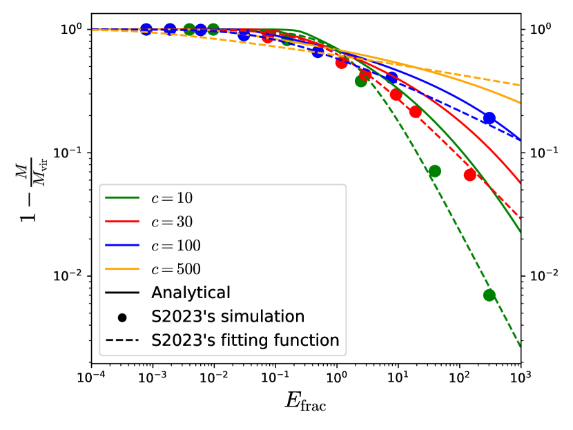
Figure 1: Survival fraction (SF) as a function of the normalized total injected energy $E_{\rm frac}$ into the minihalo as a result of stellar interaction, for concentration parameters $c=10,30,100,500$. The solid curves are the output of our implementation of K2021’s analytical approach. The dots are numerical simulation data from S2023. The dashed curves are the empirical fitting functions used by S2023.

From Fig. 1, it is clear that the analytical method described so far does not approximate the simulated data very well except for the $c=100$ case. To improve on the analytical method, we introduce a sequential stripping model for the mass loss in the minihalo.

III The sequential stripping model

One of the flaws with the expression for $\psi(x)$ as given by Eq. (13) is that it assumes that when one takes a dark matter particle from position $x$ to $\infty$, all matter in regions greater than normalized radius $x$ remains intact.

We introduce a model of dark matter particle “unbinding,” where we divide the minihalo into shells of infinitesimal thickness. During a stellar interaction, dark matter particles that will eventually be unbound will go to infinity. A dark matter particle in a particular shell that is going to infinity is not expected to feel a gravitational pull from a dark matter particle in an outer shell because shell expansion is taking place in a spherically symmetric manner. Thus, we model this as first starting with the minihalo’s outermost shell (not necessarily within the virial radius) and taking it to infinity. Then we take the next innermost shell to infinity, and so on. When we take a dark matter particle from a normalized radius $x$ to infinity, we assume that no matter exists in the region of radius $>x$ because the matter in this region has already been taken to infinity. We call this approach the “sequential stripping model”.

In Eq. (18), the upper limit of the $\epsilon$ is a minimum operation on two functions, $\psi(x)$ and $|\Delta\epsilon(x)|$. Setting $c=100$ for now, Fig. 2 shows $\psi(x)$ (according to Eq. (13)) which is a decreasing function of $x$ and $|\Delta\epsilon(x)|$ (according to Eq. (11)) which is a quadratically increasing function on $x$. The two curves intersect within or beyond the virial radius, and the normalized radius of the intersection is called the normalized crossover radius $x^{*}$.

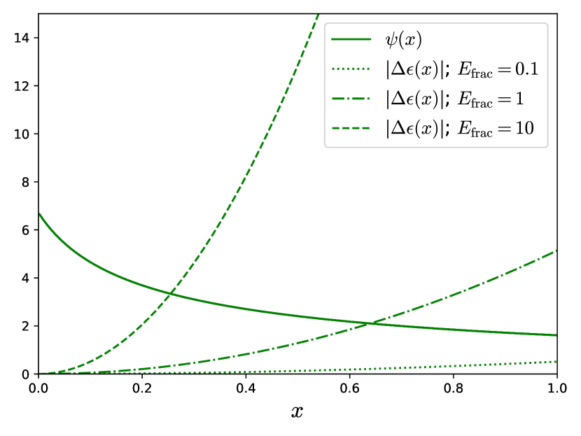
Figure 2: The normalized injected energy per unit mass $|\Delta\epsilon|$ in a minihalo due to a stellar interaction is plotted as a function of the normalized radius $x$. In doing so, the total injected energy $E_{\rm frac}$ is set to 0.1, 1, 10. The normalized relative potential $\psi$ is also plotted as a function of $x$. The $\psi(x)$ curve does not vary with $E_{\rm frac}$. In all cases for this figure, the concentration parameter $c=100$. The value of $x$ at which $|\Delta\epsilon(x)|$ and $\psi(x)$ curves intersect is called the normalized crossover radius $x^{*}$.

To make Eq. (18) more tractable, let’s utilize the normalized crossover radius, $x^{*}$, which is mathematically defined as that value of $x$ such that:

$$|\Delta\epsilon(x^{*})|=\psi(x^{*})$$ (19)

As shown in Appendix (D) the survival fraction with the sequential stripping model can be computed using

$$\text{SF}=\text{mass fraction}_{x<\min[x^{*},1]}-\text{prefactor}\times I_{\rm A}$$ (20)

where

$$\text{mass fraction}_{x<\min[x^{*},1]}=\frac{c^{2}}{f_{\rm NFW}(c)}\int\limits_{x=0}^{\min[x^{*},1]}\frac{x}{\left(1+cx\right)^{2}}\mathrm{d}x,$$ (21)

$$\text{prefactor}\equiv\frac{4\pi c^{3}}{f_{\rm NFW}(c)}$$ (22)

and

$$I_{\rm A}\equiv\int\limits_{x=0}^{\min[x^{*},1]}\int\limits_{\epsilon=0}^{|\Delta\epsilon(x)|}\ \int\limits_{\psi_{\rm B}^{\prime}=0}^{\epsilon}x^{2}\frac{1}{\sqrt{8}\pi^{2}}\ \frac{1}{\sqrt{\epsilon-\psi_{\rm B}^{\prime}}}\frac{\mathrm{d}^{2}\varrho}{\mathrm{d}\psi_{\rm B}^{\prime^{2}}}\left(x^{\prime}\left(\psi_{\rm B}^{\prime}\right)\right)\\ \sqrt{2\left(\psi_{\rm A}(x)-\epsilon\right)}\ \mathrm{d}\psi_{\rm B}^{\prime}\ \mathrm{d}\epsilon\ \mathrm{d}x.$$ (23)

The relative potentials in the above equation are given by

$$\psi_{\rm A}(x)=\frac{1}{f_{\rm NFW}(c)}\left[\frac{\ln(1+cx)}{x}-\frac{c}{1+cx^{*}}\right] ,x<x^{*}$$ (24)

and

$$\psi_{\rm B}(x)=\frac{1}{f_{\rm NFW}(c)}\left[\frac{\ln(1+cx)}{x}-\frac{c}{1+cx}\right] ,x>x^{*}.$$ (25)

Fig. 3 shows how the survival fraction (solid curves) varies with the normalized injected energy $E_{\rm frac}$. The sequential stripping model gives a better fit to the simulation data points when compared to the approach used in Fig. 1.

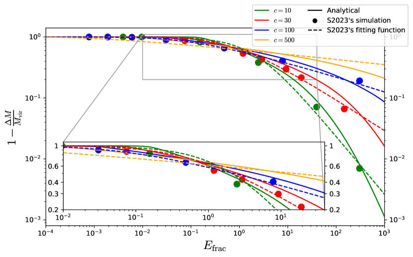
Figure 3: The same as Fig. 1 except that the solid curves are the output of our analytical approach using the sequential stripping model of mass loss in the minihalo.

III.1 The need to include relaxation

The S2023 simulation data shown in our Fig. 3, is computed after the remnant minihalo has undergone full relaxation following a stellar encounter. However, we have not accounted for this relaxation process for our analytical curves. But by juxtaposing our analytical curves with S2023’s numerical data points, it is equivalent to assuming that, in our case, the remnant minihalo relaxes to the same initial NFW profile. This is a good approximation for small $E_{\rm frac}$ values. For example, in the limit $E_{\text{frac}}\rightarrow 0$, there is no actual stellar encounter, and the resulting (relaxed) minihalo is the same NFW minihalo we started with. Thus, for small finite $E_{\rm frac}$ values, the approximation that the remnant minihalo relaxes to the same NFW profile is a good one. Thus, we see that our analytical curves have a good match to the numerical data at low values of $E_{\rm frac}$. However, S2023 finds that, in general, the remnant minihalo relaxes to a broken power profile,

$$\rho(r)=\frac{\rho_{s}}{\frac{r}{r_{s}}\left(1+\frac{r}{r_{s}}\right)^{k}},$$ (26)

which has an outer slope of $k+1$ for large values of $r$ and a slope of $1$ for small values of $r$ . For our purposes, we assume that $k=3$, and this profile is known as the Hernquist density profile [29]. Since we have argued that for small $E_{\rm frac}$, the remnant minihalo relaxes to an NFW profile, it is only for larger $E_{\rm frac}$ values that the remnant minihalo relaxes to a Hernquist profile. Since our analytical curves in Fig. 3 don’t account for this, there arises a discrepancy which becomes starker at higher values of $E_{\rm frac}$. This discrepancy leads to errors, which result in our analytical curves overshooting the numerical data points at larger $E_{\rm frac}$ values. We need to include the relaxation process in our calculations to account for this discrepancy.

III.2 The Hernquist model

In this section, we assume that after disruption, the minihalo relaxes to the Hernquist density profile, which is described by

$$\rho(r)=\frac{\rho_{\rm s}}{\frac{r}{r_{\rm s}}\left(1+\frac{r}{r_{\rm s}}\right)^{3}}$$ (27)

$$\rho(x)=\frac{\rho_{\rm s}}{cx\left(1+cx\right)^{3}}$$ (28)

Firstly, using the same sequential stripping model we used for the NFW minihalo, it can be shown that the normalized relative potential of an untruncated Hernquist minihalo is (see Appendix H)

$$\psi_{\rm A}(x)=(1+c)^{2}\biggr{[} \frac{x^{*}-x}{(1+cx^{*})(1+cx)}$$

$$+\frac{x^{*}}{(1+cx^{*})^{2}}\biggr{]} ,x<x^{*}$$ (29)

$$\psi_{\rm B}(x)=(1+c)^{2}\frac{x}{(1+cx)^{2}} ,x>x^{*}$$ (30)

To find $x^{*}$, we use the condition given in Eq. (19) where $|\Delta\epsilon(x)|$ is given by Eq. (11). The $\alpha^{2}$ and $\gamma$ for a Hernquist minihalo are given by (see Appendix I)

$$\alpha^{2}=\frac{c(6+9c+2c^{2})-6(1+c)^{2}\ln(1+c)}{c^{4}}$$ (31)

$$\gamma=\frac{4+c}{6}$$ (32)

III.3 Density profile of the first-generation minihalo resulting from stellar interaction with an NFW minihalo

We would now like to plot the density profile of the first-generation minihalo resulting from a stellar interaction of an NFW minihalo. The first-generation minihalo is assumed to have a broken power law profile (S2023). We start by specifying the scale parameters of an unperturbed NFW minihalo. Using these, we look to compute the scale parameters of the first-generation broken power law profile minihalo. We use the subscript $s$ to denote the unperturbed NFW minihalo and subscript $1$ to denote the resulting first-generation minihalo.

We first note that the NFW minihalo in the region $x>x_{\rm s}^{*}$ is completely disrupted. In addition, there is a partial mass loss in the region $x<x_{\rm s}^{*}$. One must note that $x_{\rm s}^{*}$ can be greater than 1. We first compute the total surviving mass of the NFW minihalo just after the stellar interaction. We then allow the remnant minihalo to fully relax to a broken power law profile of the form

$$\rho(r)=\frac{\rho_{1}}{\frac{r}{r_{1}}\left(1+\frac{r}{r_{1}}\right)^{k}}$$ (33)

where we are leaving $k$ unspecified for the moment, and later we will set it to 3. We use the fact that the total surviving mass of the NFW minihalo after perturbation is equal to the total mass of the fully relaxed broken power law first-generation minihalo. i.e.,

$$M_{\text{enc,s}}\left(x_{\rm s}^{*}\right)-\Delta M_{x_{\rm s}=0\rightarrow x_{\rm s}^{*}}=\lim_{x_{1}\rightarrow\infty}M_{\rm enc,1}(x_{1})$$ (34)

where $M_{\text{enc,s}}\left(x_{\rm s}^{*}\right)$ is the mass of the NFW minihalo enclosed within the normalized crossover radius $x_{\rm s}^{*}$ and $\Delta M_{x_{\rm s}=0\rightarrow x_{\rm s}^{*}}$ is the mass of the NFW minihalo lost within the normalized crossover radius $x_{\rm s}^{*}$. Also, $\lim\limits_{x_{1}\rightarrow\infty}M_{\rm enc,1}(x_{1})$ is the total mass of the first-generation broken power law minihalo. The $x_{\rm s}$ and $x_{1}$ are “local variables” of the NFW minihalo and the first-generation minihalo, respectively. They are defined as

$$x_{\rm s}\equiv\frac{r}{r_{\text{vir,s}}}$$ (35)

$$x_{1}\equiv\frac{r}{r_{\text{vir,1}}}$$ (36)

where $r_{\text{vir,s}}$ and $r_{\text{vir,1}}$ are the virial radii of the unperturbed NFW minihalo and first-generation minihalo, respectively.

We consider the disrupted halo to be a broken power law of the form

$$\rho_{k=2+\Delta}(r)=\frac{\rho_{1}}{\frac{r}{r_{1}}\left(1+\frac{r}{r_{1}}\right)^{2+\Delta}}$$ (37)

for a parameter $\Delta>0$.

We now look at Fig. 6 of S2023 and make the reasonable assumption that at small radii, the unperturbed NFW minihalo density profile and the first-generation Hernquist/broken power-law density profile are indistinguishable from each other. We write this as

$$\lim_{r\rightarrow 0}\rho_{\rm NFW}(r) =\lim_{r\rightarrow 0}\rho_{k=2+\Delta}(r)$$

$$\lim_{r\rightarrow 0}\frac{\rho_{\rm s}}{\frac{r}{r_{\rm s}}\left(1+\frac{r}{r_{\rm s}}\right)^{2}} =\lim_{r\rightarrow 0}\frac{\rho_{1}}{\frac{r}{r_{1}}\left(1+\frac{r}{r_{1}}\right)^{2+\Delta}}$$

$$\frac{\rho_{\rm s}}{\frac{r}{r_{\rm s}}} =\frac{\rho_{1}}{\frac{r}{r_{1}}}$$

$$\Rightarrow\rho_{\rm s}r_{\rm s} =\rho_{1}r_{1}$$ (38)

As shown in Appendix J we can compute $r_{1}$ in terms of $r_{\rm s}$ as follows

$$r_{1} =r_{\rm s}\times R_{\rm s}$$ (39)

where

$$R_{\rm s}\equiv\sqrt{(\Delta+\Delta^{2})\left[f_{\rm NFW}(c_{\rm s}x_{\rm s}^{*})-4\pi c_{\rm s}^{3}I_{\rm s}\right]}$$ (40)

and

$$c_{\rm s}\equiv\frac{r_{\rm vir,s}}{r_{\rm s}}.$$ (41)

It is also shown in the same appendix that

$$\rho_{1}=\frac{\rho_{\rm s}}{R_{\rm s}}$$ (42)

Thus, if the scale parameters $\rho_{\rm s}$, $r_{\rm s}$ of the NFW profile are given, Eqs. (39) and (42) give the scale parameters $\rho_{1}$, $r_{1}$ of the resulting first-generation broken power law minihalo.

Using N-body simulations, S2023 finds that when an NFW minihalo participates in a stellar interaction with impact parameter $b=2\times 10^{-5}\mathrm{kpc}$, the resulting first-generation minihalo will have a broken power law profile with $k=3.2$ or $\Delta=1.2$. In such a case,

$$R_{\rm s}=\sqrt{\frac{66}{25}\left[f_{\rm NFW}(c_{\rm s}x_{\rm s}^{*})-4\pi c_{\rm s}^{3}I_{\rm s}\right]}$$ (43)

On the other hand, according to the N-body simulations of S2023, if the impact parameter is $b=5\times 10^{-5}\mathrm{kpc}$, the resulting first-generation minihalo will have a broken power law profile with $k=3.3$ or $\Delta=1.3$. Then,

$$R_{\rm s}=\sqrt{\frac{299}{100}\left[f_{\rm NFW}(c_{\rm s}x_{\rm s}^{*})-4\pi c_{\rm s}^{3}I_{\rm s}\right]}$$ (44)

Finally, assuming for simplicity, that the first-generation minihalo had a Hernquist profile ($k=3$ or $\Delta=1$),

$$R_{\rm s}=\sqrt{2f_{\rm NFW}(c_{\rm s}x_{\rm s}^{*})-8\pi c_{\rm s}^{3}I_{\rm s}}$$ (45)

Moving on, instead of specifying the unperturbed NFW minihalo by its two scale parameters, we would like to specify it by two other quantities: its concentration parameter and its virial mass. So, in order to compute the scale parameters of the first-generation minihalo, we need to first compute the scale parameters of the NFW minihalo from its concentration and virial mass.

We first use the definition of the virial radius of the NFW minihalo. The virial radius is that radius at which the average density $\bar{\rho}_{\rm vir}$ enclosed within the virial radius is 200 times the critical density $\rho_{\rm crit}$ of the universe. Therefore,

$$\frac{\text{Mass within virial radius}}{\text{Volume within virial radius}} =200\rho_{\rm crit}$$

$$\ \frac{\int\limits_{r=0}^{r_{\rm vir,s}}\rho_{\rm NFW}(r)\times 4\pi r^{2}dr}{\frac{4\pi}{3}r_{\rm vir,s}^{3}} =200\rho_{\text{crit }}$$ (46)

Let

$$x_{s}\equiv\frac{r}{r_{\text{vir,s}}}\ \Rightarrow\ r=x_{\rm s}r_{\text{vir,s }}$$ (47)

Substituting Eq. (47) in Eq. (III.3)

$$\int\limits_{x_{\rm s}=0}^{1}\rho_{\rm NFW}\left(x_{\rm s}\right)x_{\rm s}^{2}\mathrm{d}x_{\rm s}=\frac{200}{3}\rho_{\text{crit}}$$ (48)

Substituting Eq. (4) in Eq. (48) and performing the integration with respect to $x_{\rm s}$ in the L.H.S. of Eq. (48), we get

$$\frac{\rho_{\rm s}}{c^{3}}\left[\ln(1+c)-\frac{c}{1+c}\right]=\frac{200}{3}\rho_{\rm crit}$$

$$\Rightarrow\rho_{\rm s}=\frac{200}{3}\frac{c^{3}}{f_{\rm NFW}(c)}\rho_{\rm crit}$$ (49)

Cosmological observations [30] fix the value of $\rho_{\rm crit}$ as

$$\rho_{\text{crit}}=1.3483\times 10^{-7}\mathrm{M}_{\odot}/\mathrm{pc}^{3}$$ (50)

Thus, specifying the concentration of the NFW minihalo fixes its scale density through Eq. (49).

Next, the average density within the virial radius of the NFW minihalo is expressed in terms of its virial mass and viral radius as follows

$$\bar{\rho}_{\text{vir}}=\frac{M_{\text{vir,s}}}{\frac{4\pi}{3}r_{\text{vir,s}}^{3}}$$ (51)

Substituting Eq. (41) in Eq. (51) and solving for $r_{\rm s}$, we get

$$r_{\rm s}=\frac{1}{c_{\rm s}}\left(\frac{3M_{\text{vir,s}}}{4\pi\bar{\rho}_{\text{vir}}}\right)^{1/3}$$ (52)

Noting that by definition

$$\bar{\rho}_{\rm vir}=200\rho_{\text{crit}}$$ (53)

Therefore, Eq. (52) becomes

$$r_{\rm s}=\frac{1}{c_{\rm s}}\left(\frac{3M_{\rm vir,s}}{800\pi\rho_{\text{crit}}}\right)^{1/3}$$ (54)

Thus, given the concentration and virial mass of the NFW minihalo, its scale parameters can be found using Eqs. (49) and (54).

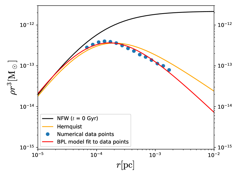
(a)

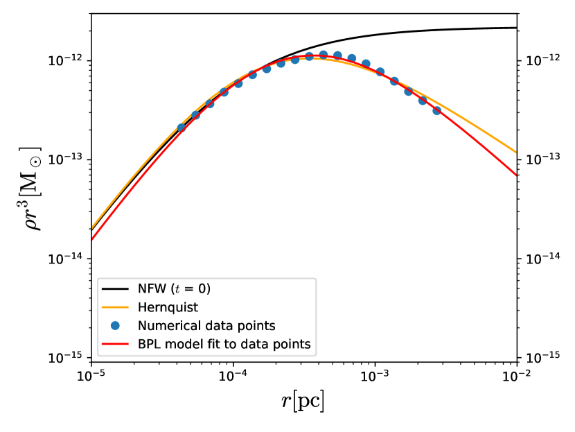
(b)

Figure 4: The left and right panels show the density profile of an NFW minihalo (black curve) which has a stellar encounter with impact parameters $b=2\times 10^{-5}\rm kpc$ and $b=5\times 10^{-5}\rm kpc$ respectively. The NFW minihalo has an initial concentration $c=100$ and virial mass $M_{\rm vir}=10^{-10}\rm M_{\odot}$. The orange curve shows the case where the remnant minihalo has relaxed to a Hernquist density profile, which is a broken power law profile with $k=3$. The teal dots are numerical data points of the resulting density profile stabilized at $t=2.5$ Gyr post-stellar interaction taken from S2023. We performed a curve fit of these data points to a broken power law profile and obtained its three parameters. The broken power law profile is shown as the red curves.

Given the concentration and virial mass of the unperturbed NFW minihalo, we are now able to plot the density profile of the first-generation minihalo. We use $c_{\rm s}=100$ and $M_{\text{vir,s}}=10^{-10}\rm M_{\odot}$. The left (right) panel of Fig. 4 shows the case where the impact parameter $b=2\times 10^{-5}\mathrm{kpc}$ ($b=5\times 10^{-5}\mathrm{kpc}$). The black curve shows the density profile of the unperturbed NFW minihalo while the orange curve shows the case where the fully relaxed first-generation minihalo is assumed to have a Hernquist profile $(k=3)$. For both the impact parameter cases, S2023 numerically shows how the density profile of the resulting minihalo changes and stabilizes over time. We chose the data points on that portion of the density profile curve at $t$ = 2.5 Gyr where the profile had stabilized and used these datapoints to find the model parameters of the resulting broken power law of the form given in Eq. (33). These data points are shown in teal in both panels of Fig. 4. We did a least squares fit of the data points and obtained the optimal parameters $r_{1}$, $\rho_{1}$ and $k$. These parameters are given in Table 1. The resulting broken power law profiles are plotted as the red curves in Fig. 4. We notice that the broken power law profile merges with the NFW profile at small radii. This further reinforces our assumption that the parent and relaxed child AMCs are indistinguishable at small radii during a stellar interaction. Next, we calculated the virial radius $r_{\rm vir,s}$ of the unperturbed NFW minihalo using Eq. (51). We found that $r_{\rm vir,s}=9.6\times 10^{-3}$pc. We then calculated the masses of the Hernquist and broken power law profiles inside this virial radius $r_{\rm vir,s}$. The ratio of the above mass to the virial mass of the NFW profile then gives us the survival fraction of the Hernquist or broken power-law profiles. Alternatively, we also calculate the value of normalized injected energy $E_{\rm frac}$ using the impact parameter using Eq. (9). Knowing $E_{\rm frac}$, we calculate the survival fraction according to S2023’s empirical response function. These survival fractions are presented in Table 1. As can be seen, there is about a 0.03 difference in the SF value between the broken power law case and the SF from S2023’s empirical response function. This is indicative of the level of systematic error in determining the SF. As can be seen, the difference between the SF from the Hernquist and the broken power law profiles is around 0.01, which indicates that within the level of systematic error, the Hernquist profile could be used instead of the broken power law.

b	$2\times 10^{-5}$kpc	$5\times 10^{-5}$kpc
$r_{1}$	$1.14\times 10^{-4}$pc	$2.47\times 10^{-4}$pc
$\rho_{1}$	$2.44$M⊙/pc3	$0.716$M⊙/pc3
$k$	3.38	3.34
SF from Hernquist	0.15	0.433
SF from BPL	0.137	0.423
SF from S2023 response function	0.172	0.393

Table 1: An NFW profile minihalo of concentration $c_{\rm s}$ and virial mass $M_{\rm vir,s}$ undergoes a stellar interaction with two different impact parameters $b=2\times 10^{-5}\mathrm{kpc}$ and $b=5\times 10^{-5}\mathrm{kpc}$. In each case, we fit the numerical data points in Fig. 4 to obtain the parameters of the resulting broken power law (BPL) profile. The scale radius $r_{1}$, scale density $\rho_{1}$, and power parameter $k$ of the BPL profile are presented above. Moreover, the survival fractions using the Hernquist and BPL profiles in Fig. 4 as well as using S2023’s empirical response function are presented.

III.4 Incorporating relaxation to a Hernquist profile

We now try to improve upon Fig. 3, this time incorporating the relaxation process to a Hernquist profile. We assume we are given the concentration $c_{\rm s}$ of the unperturbed NFW minihalo. Then, Eq. (49) gives us the scale density $\rho_{\rm s}$ of the NFW minihalo. Having calculated $\rho_{\rm s}$, Eq. (42) gives us the scale density $\rho_{1}$ of the relaxed first-generation Hernquist minihalo, where $r_{\rm s}$ is given by Eq. (45)

Our next task is to compute the concentration $c_{1}$ of the first-generation Hernquist minihalo and get an equation analogous to Eq. (49) but for the Hernquist profile. We start with the definition of the virial radius as before. This then leads us to an equation similar to Eq. (48) but for the first-generation Hernquist minihalo, finally resulting in an equation relating the concentration $c_{1}$ and scale density $\rho_{1}$ as follows (see Appendix L.1):

$$\frac{1}{2c_{1}\left(1+c_{1}\right)^{2}}=\frac{200}{3}\frac{\rho_{\text{crit}}}{\rho_{1}}$$ (55)

The survival fraction after relaxation is given by (see Appendix K)

SF $$\equiv\frac{M_{\text{enc,1}}\left(x_{1}^{r_{\rm vir,s}}\right)}{M_{\text{vir,s}}}$$ (56)

$$=\frac{1}{2}R_{\rm s}^{2}\frac{f_{\rm Hern}(c_{1}x_{1}^{r_{\text{vir,s}}})}{f_{\rm NFW}(c_{\rm s})}$$ (57)

where

$$f_{\rm Hern}(x)=\frac{x^{2}}{(1+x)^{2}}$$ (58)

$$x_{1}^{r_{\rm vir,s}}\equiv\frac{r_{\rm vir,s}}{r_{\rm vir,1}}$$ (59)

is the virial radius of the unperturbed NFW minihalo expressed in terms of the “local” normalized radial distance variable of the first-generation Hernquist minihalo. $M_{\rm enc,1}$ is the mass enclosed for a Hernquist profile. $x_{1}^{r_{\text{vir,s}}}$ can be written as (see Appendix K)

$$x_{1}^{r_{\text{vir,s}}}=\frac{c_{\rm s}}{c_{1}}\frac{1}{R_{\rm s}}$$ (60)

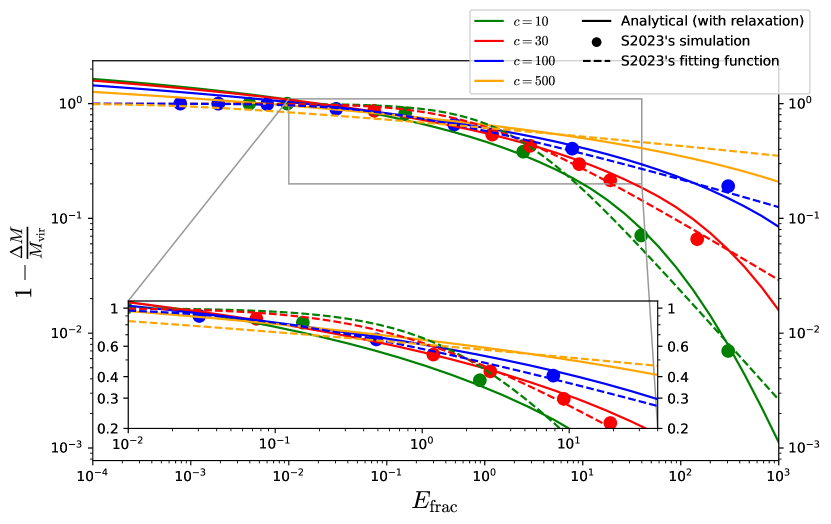
Figure 5: The same as Fig. 1 except that the solid curves are the output of our analytical approach using the sequential stripping model of mass loss in the minihalo and taking into account relaxation of the remnant minihalo to a Hernquist profile.

Using this procedure, the survival fraction can be computed against $E_{\rm frac}$. Fig. 5 shows the results. The solid lines are our analytical curves. The circular dots are numerical data points from S2023. The dashed curves are S2023’s curve fits to the numerical data. Our analytical curves closely match the numerical data points for larger values of $E_{\rm frac}$. This is because it is a reasonable assumption that the remnant minihalo relaxes to a Hernquist profile in this regime. However, our analytical curves overshoot the numerical data for smaller values of $E_{\rm frac}$. This is because, as discussed in Section III.1, for smaller $E_{\rm frac}$ values, it is a better approximation to assume that the remnant minihalo relaxes to the same NFW profile, not the Hernquist profile.

III.5 The switching procedure

Fig. 3 shows that the sequential striping model without considering relaxation produces a good match to the numerical data at low values of $E_{\rm frac}$ but overshoots the data at high $E_{\rm frac}$ values. On the other hand, Fig. 5 shows that the sequential stripping model incorporating relaxation to a Hernquist profile overshoots the numerical data at low values of $E_{\rm frac}$ but is a good match at high $E_{\rm frac}$ values. We have previously discussed the physical intuitions for both these models. We now introduce a switching procedure where, for any given $E_{\rm frac}$ value, we compute the survival fraction both without and with considering relaxation to a Hernquist profile, and we choose the method that gives us the lesser value of survival fraction. Implementing this procedure in Python, we find that the algorithm selects the method without relaxation for low values of $E_{\rm frac}$. As $E_{\rm frac}$ is increased, the algorithm switches to the method with relaxation at some (unenforced) value of $E_{\rm frac}$.

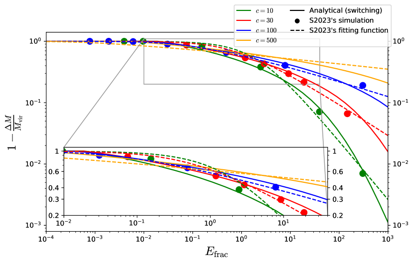
Figure 6: The same as Fig. 1 except that the solid curves are the output of our analytical approach using the sequential stripping model of mass loss in the minihalo and incorporating the switching procedure.

Fig. 6 shows the survival fraction plotted against $E_{\rm frac}$ using the switching procedure. The switching procedure provides a good match to the numerical data for all regimes of $E_{\rm frac}$ values considered.

Figure 7: The error in a model is defined as (model - data). Plotted are the errors in the output of Ref. [21]’s (K2021) analytical approach, our analytical switching procedure and S2023’s empirical fitting functions. The numerical data is taken from S2023’s N-body simulations. Errors are plotted for concentration parameters $c=10,30,100$.

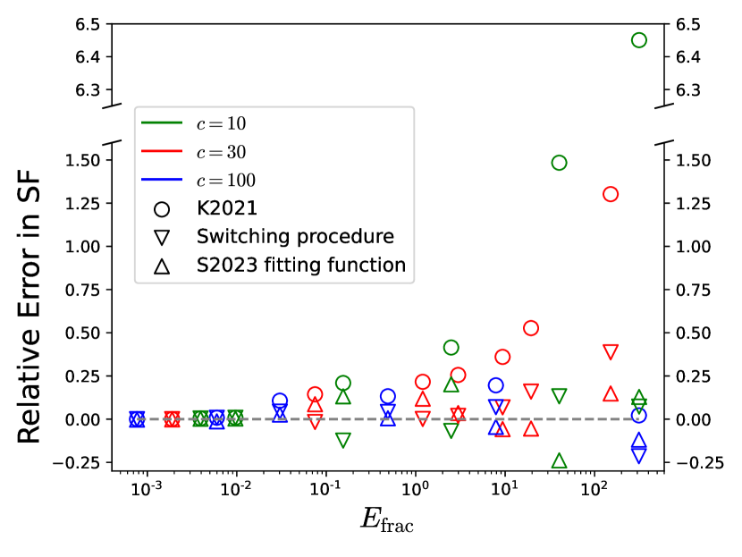
Figure 8: The same as Fig. 7 except for the relative error, which is defined as (model - data)/data, rather than the error.

Figs. 7 and 8 show the error and relative error respectively in the survival fraction vs $E_{\rm frac}$ curves for K2021’s approach, our analytical switching procedure and S2023’s fitting functions.

As can be seen, the smallest errors are shown by the switching procedure and S2023’s semi-analytic fitting functions. In some instances, the switching procedure outperforms S2023’s fitting functions.

IV Multiple stellar encounters of an NFW minihalo

Here, we consider the scenario of multiple successive stellar interactions with an NFW minihalo. After each stellar interaction, the remnant minihalo is allowed to fully relax before the next stellar interaction is applied. S2023 states that after a stellar encounter, the NFW minihalo will relax to a broken power law profile with a $k$ dependent on the impact parameter of the stellar interaction. In general, $k\sim 3$. We will assume $k=3$ for our analytical calculations, i.e., a Hernquist profile. We also assume that when a Hernquist profile is perturbed, the remnant minihalo will relax to a Hernquist profile with a different concentration and overall mass.

The NFW and Hernquist density profiles are two-parameter models. However, it turns out that we need only one piece of information to calculate the survival fraction (or mass loss fraction) due to a stellar encounter. Here, we use the concentration of the minihalo as that piece of information. As we will see later, the concentration of a two-parameter minihalo, like the NFW and Hernquist profiles, uniquely determines the scale density of that minihalo. So, we cannot compute the exact value of the scale radius as that would need a second piece of information. However, we can compute the ratio of the parent and child minihalos scale radii. This will allow us to calculate the scale density of the child minihalo. Knowing the scale density of the child minihalo gives us its concentration parameter. We then iterate this process to get the concentrations (and hence survival fractions) of successive generations of minihalos.

We use the subscript $s$ to denote the unperturbed NFW minihalo. We use the numeral $n$ to denote the $n^{\text{th }}$ generation Hernquist minihalo, where the first-generation Hernquist minihalo is the child of the NFW minihalo and the $n^{\text{th }}$ generation Hernquist minihalo is the child of the $(n-1)^{\text{th }}$ generation Hernquist minihalo.

To compare the survival fractions of successive generations of minihalos, we will define the survival fraction of any minihalo as

$$\text{SF}_{n}\equiv 1-\frac{\Delta M}{M_{\text{vir,s}}}$$ (61)

where $n=s,1,2,3,\cdots$ and $\Delta M$ is the total mass lost within the virial radius of the unperturbed NFW minihalo. This means that our region of interest for the purposes of evaluating mass loss is always inside a sphere of radius $r_{\rm vir,s}$.

We start the procedure by specifying the concentration $c_{\rm s}$ of the NFW minihalo. To better understand how some of the equations in this section are derived, see Appendix L.

Step I: Compute the survival fraction of the NFW minihalo

We use the switching procedure to find out the survival fraction of the NFW minihalo. We will restrict our incremental $E_{\rm frac}$ to be high enough such that the switching procedure forces the remnant minihalo to relax to a Hernquist profile. Knowing $c_{\rm s}$, we can calculate the scale density $\rho_{\rm s}$ of the NFW minihalo using Eq. (49). Next we calculate $R_{\rm s}$ using Eq. (45). We can then calculate the scale density $\rho_{1}$ of the first-generation Hernquist minihalo using Eq. (42). We can then calculate concentration $c_{1}$ of the first-generation Hernquist minihalo by solving for Eq. (55). The NFW minihalo’s survival fraction is then given by Eq. (56).

Step II: Compute the survival fraction of the $n^{\rm th}$ generation Hernquist minihalo ($n\geq 1$)

In the $(n-1)^{\text{th}}$ step, we would have calculated the scale density $\rho_{n}$ and concentration $c_{n}$ of the $n^{\rm th}$ generation Hernquist minihalo. We next consider the conservation of mass condition for the transition from the $n^{\text{th}}$ to $(n+1)^{\text{th}}$ generation Hernquist minihalo.

$$M_{\text{enc,}n}\left(x_{n}^{*}\right)-\Delta M_{x_{n}=0\rightarrow x_{n}^{*}}=\lim_{x_{n+1}\rightarrow\infty}M_{\text{enc,}n+1}\left(x_{n+1}\right)$$ (62)

Evaluating each of the terms in Eq. (62), it can be shown that the ratio of the scale radii of the $(n+1)^{\text{th}}$ to the $n^{\text{th}}$ generation Hernquist minihalos is (see Appendix L.3)

$$\frac{r_{n+1}}{r_{n}}=R_{n}$$ (63)

where

$$R_{n}\equiv\sqrt{f_{\rm Hern}(c_{n}x_{n}^{*})-8\pi c_{n}^{3}I_{n}}$$ (64)

$$I_{n}\equiv\int\limits_{x_{n}=0}^{x_{n}^{*}}\int\limits_{\epsilon=0}^{|\Delta\epsilon(x_{n})|}\int\limits_{\psi_{\rm B}^{\prime}=0}^{\epsilon}\frac{1}{\sqrt{8}\pi^{2}}x_{n}^{2}\sqrt{2(\psi_{\rm A}(x_{n})-\epsilon)}\\ \frac{1}{\sqrt{\epsilon-\psi_{\rm B}^{\prime}}}\frac{\mathrm{d}^{2}\varrho}{\mathrm{d}\psi_{\rm B}^{\prime^{2}}}\left(x_{n}^{\prime}(\psi_{\rm B}^{\prime})\right)\mathrm{d}\mathrm{\psi_{\rm B}^{\prime}}\mathrm{d}\epsilon\mathrm{d}x_{n}$$ (65)

We can now calculate the scale density $\rho_{n+1}$ of the $(n+1)^{\text{th}}$ generation Hernquist minihalo using the following relationship (see Appendix L.3):

$$\rho_{n+1}=\frac{\rho_{n}}{R_{n}}$$ (66)

Next, we compute the concentration $c_{n+1}$ of the $(n+1)^{\text{th}}$ generation Hernquist minihalo by adapting Eq. (55) and solving for $c_{n+1}$ in the expression below:

$$\frac{1}{2c_{n+1}\left(1+c_{n+1}\right)^{2}}=\frac{200}{3}\frac{\rho_{\rm crit}}{\rho_{n+1}}$$ (67)

The survival fraction of the $n^{\text{th}}$ generation Hernquist minihalo is given by (See Appendix L.4)

$$\text{SF}_{n}=\frac{1}{2}\left(R_{n}R_{n-1}\ldots R_{1}R_{\rm s}\right)^{2}\frac{f_{\rm Hern}(c_{n+1}x_{n+1}^{r_{\text{vir,s}}})}{f_{\rm NFW}(c_{\rm s})}$$ (68)

where

$$x_{n+1}^{r_{\text{vir,s}}}=\frac{c_{\rm s}}{c_{n+1}}\frac{1}{R_{n}R_{n-1}\cdots R_{1}R_{\rm s}}$$ (69)

Step II is applied for $n=1$, then $n=2$, and so on. This completes the theoretical procedure for computing survival fractions for multiple stellar encounters of an NFW minihalo.

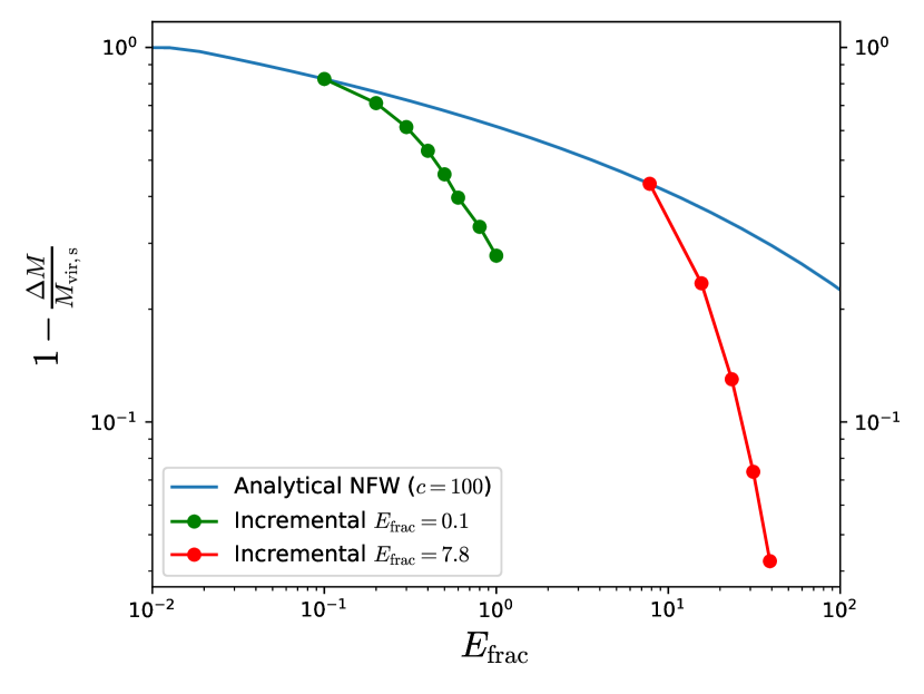
Figure 9: The survival fraction of an NFW minihalo is plotted against the total normalized injected energy $E_{\rm frac}$. The blue curve shows the case of a single stellar encounter. The green (red) curves represent the multiple stellar encounter scenario where an incremental $E_{\rm frac}=0.1(7.8)$ is used repeatedly. When the incremental $E_{\rm frac}$ is higher (red curve), the deviation from the single energy injection case (blue curve) is higher as well.

We now set $c_{\rm s}=100$ and evaluate the survival fractions of the NFW minihalo and successive generations of Hernquist minihalos using the above mentioned procedure. Fig. 9 shows the survival fractions resulting from multiple energy injections into the minihalo due to successive stellar encounters. The blue curve represents the survival fraction vs $E_{\rm frac}$ due to single stellar encounter scenarios. The green/red curves represent multiple encounters, each characterized by an incremental $E_{\rm frac}=0.1/7.8$, respectively. However, the green curve’s last two incremental energy injections are characterized by an $E_{\rm frac}=0.2$.

It can be seen that multiple encounters generate more mass loss than a single-shot encounter case of the same cumulative energy injection $E_{\rm frac}$.

In Fig. 9, we have fixed the incremental $E_{\rm frac}$ between successive encounters. According to S2023, for a large enough impact parameter,

$$E_{\rm frac}=\frac{\alpha^{2}}{\pi\gamma}\frac{GM_{\star}^{2}}{V^{2}b^{4}}\frac{1}{\bar{\rho}_{\rm vir}}$$ (70)

where $M_{\star}$ is the mass of the perturbing star, $V$ is the relative velocity of the star, and $\bar{\rho}_{\rm vir}$ is the average density of the minihalo within its virial radius. $\alpha^{2}$ and $\gamma$ are functions of $c$, which depends on the density profile of the minihalo - specifically, it depends on the scale density of the minihalo. Between successive encounters of the minihalo, its density profile changes. Thus, the ratio $\frac{\alpha^{2}}{\gamma}$ changes. Assuming we fix $M_{\star}$, $V$ and $\bar{\rho}_{\rm vir}$ between encounters (recall $\bar{\rho}_{\rm vir}=200\rho_{\text{crit}}$, so it is fixed), fixing $E_{\rm frac}$ necessarily means that the impact parameter $b$ changes between successive encounters.

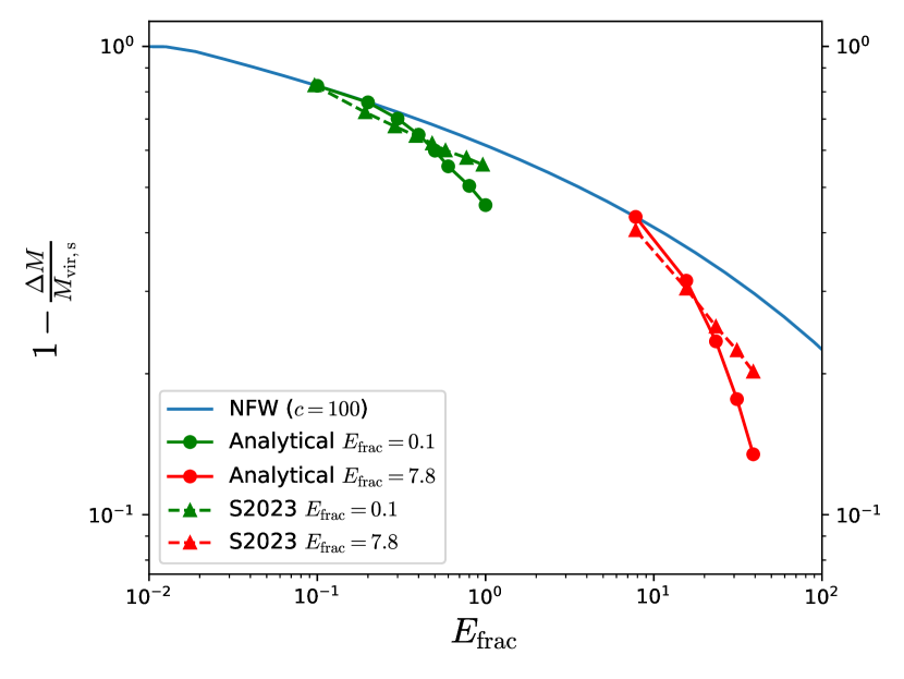
Figure 10: The survival fraction of an NFW minihalo is plotted against the total normalized injected energy $E_{\rm frac}$. The blue curve shows the case of a single stellar encounter. The green (red) curves represent the multiple stellar encounter scenario where an incremental $E_{\rm frac}=0.1(7.8)$ is used repeatedly. The solid curves with circular markers represent the output of our analytical method, while the dashed curves with triangular markers represent the output of S2023’s N-body simulations.

In Fig. 9 of S2023, they have a graph where they use their N-body results to evaluate the survival fractions of an NFW minihalo for a multiple stellar encounter scenario. We would like to compare our results with that of S2023. They use incremental $E_{\rm frac}=0.1,0.1,0.1,0.1,0.1,0.1,0.2,0.2$ in one case and $E_{\rm frac}=7.8,7.8,7.8,7.8,7.8$ in a second case. We will also use these values of incremental $E_{\rm frac}$ in our analytical calculations. S2023 evaluates $b$ from Eq. (70) for an NFW profile, given knowledge of the concentration of the NFW minihalo and the $E_{\rm frac}$ value. S2023 then fixes $b$ between successive encounters while simultaneously assuming that $E_{\rm frac}$ is held constant $(0.1/0.2/7.8)$ [31]. This approach is inaccurate since the density profile of the minihalo changes between encounters, thus changing the ratio $\frac{\alpha^{2}}{\gamma}$. Thus, both $E_{\rm frac}$ and $b$ can’t be fixed between encounters. As we mentioned, S2023 fixes $b$ between successive encounters. To compare the output of our analytical procedure to S2023’s results, we emulate this by first evaluating $b$ from Eq. (70) for the NFW profile, with a known $E_{\rm frac}$ $(0.1/0.2/7.8)$ and then fix that value of $b$ and evaluate the actual $E_{\rm frac}$ using Eq. (70) for the remaining encounters. Using the actual value of $E_{\rm frac}$ for each encounter, we analytically compute the survival fraction for that encounter. However, when plotting the results in a graph, we use $E_{\rm frac}=0.1/0.2/7.8$ for each encounter instead of the actual value of $E_{\rm frac}$. This allows us to compare the output of our analytical procedure to the numerical simulations of S2023. Fig. 10 shows the corresponding results. The blue curve represents the single encounter case. The green (red) curves represent the multiple encounter scenario with incremental $E_{\rm frac}=0.1(7.8)$. The solid curves with circular markers represent our analytical method, while the dashed curves with triangular markers represent S2023’s numerical simulations. There is a fair amount of agreement between our results and S2023’s. However, the slight deviation in the two results is likely because, as is apparent from Fig. 6, our analytical method of computing survival fractions gives a slightly different answer compared to S2023’s numerical simulations. Moreover, we assume that the successive generations of minihalos have Hernquist density profiles. However, in reality, those minihalos will have a broken power law profile with the $k$ parameter close to, but not exactly, 3 (which would be the Hernquist profile).

V Empirical method of accounting for multiple encounters

Inspired by ref. [32], we propose the following empirical method for evaluating the effective single energy injection from multiple stellar encounters:

$$E_{\rm frac,eff}=\left(\sum_{i}E_{{\rm frac},i}^{p/2}\right)^{2/p}$$ (71)

where $p$ is a parameter to be determined. For $p=2$, the value of $E_{\rm frac,eff}$ would correspond to the sum of all individual $E_{{\rm frac},i}$. For $p<2$, multiple energy injections would have an enhanced effect. Only the strongest energy injection would matter for $p\rightarrow$ $\infty$.

Ref. [32] finds that $p=1.2$ for a prompt cusp which has a density that differs from the NFW form, following a steep $r^{-1.5}$ density profile between outer boundary set by the curvature of the initial density peak and inner core determined by the physical nature of the dark matter. S2023 effectively assumed $p=2$. As our results in the previous section indicate, $p<2$ would provide a better fit. A similar finding was obtained by ref. [28]. However, due to the different methods and assumptions used there, it is difficult to make a precise comparison between our results.

We performed a least squares fit to find the optimal value of $p$ for the cases we investigated in Figs. 9. The results are shown in Fig. 11. Our best-fit values of $p=0.8$ and $p=0.6$ are consistent with our earlier findings that successive encounters are more destructive than a single effective encounter, with the effective relative energy equal to the sum of the effective energies of each actual encounter.

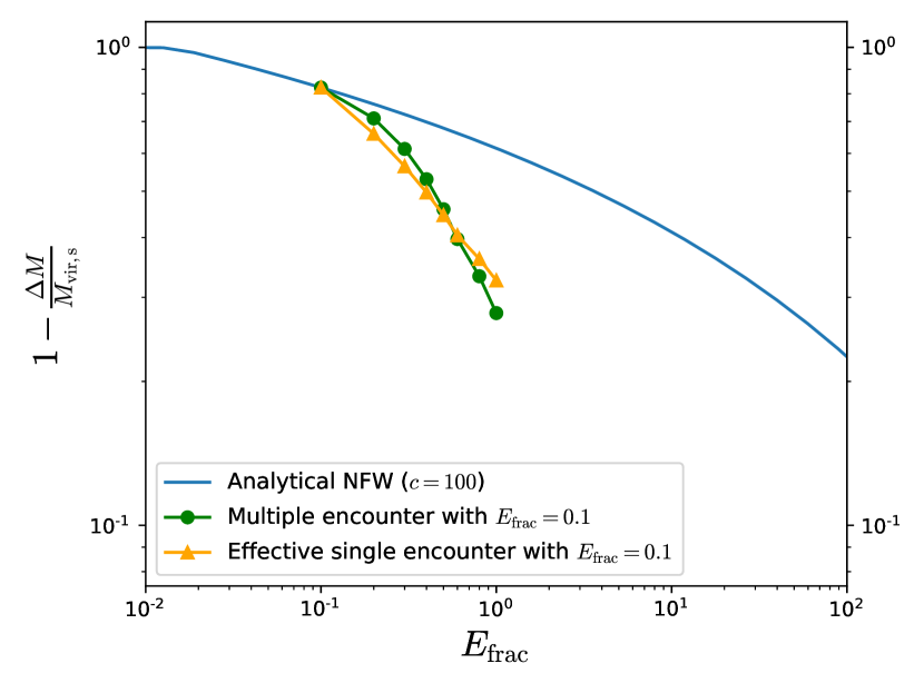
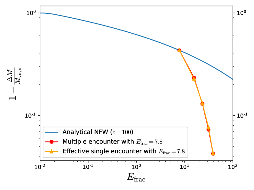
Figure 11: The survival fraction (SF) of an NFW minihalo is plotted against the total normalized energy energy injection $E_{\rm frac}$. The blue curve shows the case of a single stellar encounter. The green (red) curves represent the multiple stellar encounter scenario where an incremental $E_{\rm frac}=0.1(7.8)$ is used repeatedly. In the top and bottom panels, the orange curve is the best fit $p$ using Eq. 71 for individual energy injections of $E_{\rm frac}=0.1$ and 7.8, respectively. The respective best-fit values of $p$ were 0.8 and 0.6.

VI Discussion and Conclusions

In extending the K2021 method for evaluating minihalo mass loss due to stellar encounters, we have introduced a sequential stripping model. This model conceptually divides the minihalo into infinitesimally thin shells, sequentially focusing from the outermost to the innermost. However, this sequential approach does not imply a temporal sequence in the stripping process. Instead, it is a methodological tool for analysis. In reality, during a stellar encounter, the stripping of shells occurs simultaneously, regardless of their distance from the minihalo center.

Building on this, it is crucial to note that our model also accounts for changes in the minihalo’s profile after a stellar encounter. This aspect becomes significant if the energy injection during the encounter is sufficiently large, altering the minihalo’s structure and dynamics.

As shown in Figs. 7 and 8, our new method provides a significantly better fit to S2023’s N-body simulation results compared to the K2021 method. This is particularly noticeable for $E_{\rm frac}\gtrsim 10^{-2}$, which is relevant for modeling the mass loss incurred by multiple passes through the Milky Way disk (S2023).

A significant finding of our research centers on the treatment of minihalos undergoing multiple stellar encounters. Note that this is for the case where the minihalo has had time to stabilize after each encounter. As discussed in S2023, for example, this scenario is appropriate for successive cases of the minihalo passing through the Galactic disk. Although many encounters may occur during a single passing through of the disk, these will be in such rapid succession that they can be considered one encounter where the energies have been summed up to give the effective energy of one encounter.

Contrary to the results presented by S2023, our analysis suggests that sequential stellar interactions lead to a more pronounced mass loss in minihalos when they are allowed to fully relax between encounters. This finding will have implications for our understanding of minihalo survival and evolution in dense stellar environments. S2023 found that by $z=0$ at the Solar System location, around 60% of the mass in minihalos has survived stellar disruption from the Milky Way disk. However, as we have shown, they assume the fractional energy injections for each passage through the disk can be added to make a single effective fractional energy injection. Our results indicate that this underestimates the effects of sequential energy injections. In future work, we would like to use our new method of evaluating the impact of sequential stellar encounters to estimate the mass lost by minihalos in the Milky Way.

Appendix A Computing the expression for the normalized relative potential of an untruncated NFW minihalo

The Newtonian gravitational potential for an untruncated NFW density profile is Ref. [20, equation 2.67]

$$\Phi(r)=-4\pi G\rho_{\rm s}r_{\rm s}^{3}\frac{\ln\left(1+\frac{r}{r_{\rm s}}\right)}{r}$$ (72)

Making the substitutions $\frac{r}{r_{\rm s}}=\frac{xr_{\rm vir}}{r_{\rm s}}=cx$ and $r_{\rm s}=\frac{r_{vir}}{c}$ in Eq. (72)

$$\Phi(x) =-4\pi G\rho_{\rm s}\frac{r_{\rm vir}^{3}}{c^{3}}\frac{\ln\left(1+cx\right)}{xr_{\rm vir}}$$

$$=-\Psi_{0}\times\frac{4\pi\rho_{\rm s}r_{\rm vir}^{3}}{M_{\rm vir}c^{3}}\frac{\ln\left(1+cx\right)}{x}$$ (73)

where $\Psi_{0}\equiv\frac{GM_{\rm vir}}{r_{\rm vir}}$

Substituting for $M_{\rm vir}$ from Eq. (E) in Eq. (A)

$$\Phi(x)=-\Psi_{0}\frac{1}{f_{\rm NFW}(c)}\frac{\ln\left(1+cx\right)}{x}$$ (74)

Let the relative potential be $\Psi\equiv-\Phi$ and the normalized relative potential be $\psi\equiv\frac{\Psi}{\Psi_{0}}$. $\implies\psi=-\frac{\Phi}{\Psi_{0}}$. From Eq. (74), this implies that the normalized relative potential is

$$\psi(x)=\frac{1}{f_{\rm NFW}(c)}\frac{\ln\left(1+cx\right)}{x}$$ (75)

Appendix B Computing the dimensionless expression for the survival fraction of an NFW minihalo

We start with Eq. (15). Substituting with $r=xr_{\rm vir}$, $\Psi=\psi\Psi_{0}$, $\varepsilon=\epsilon\Psi_{0}$, $|\Delta\varepsilon|=|\Delta\epsilon|\Psi_{0}$ and $f=\frac{\rho_{\rm s}}{\Psi_{0}^{3/2}}\hat{f}$, we get

$$\Delta M=16\pi^{2}\rho_{\rm s}r_{\rm vir}^{3}\int\limits_{x=0}^{1}\mathrm{d}x\ x^{2}\int\limits_{\epsilon=0}^{\min\left[|\Delta\epsilon(x)|,\psi(x)\right]}\mathrm{d}\epsilon\\ \sqrt{2(\psi(x)-\epsilon)}\hat{f}(\epsilon)$$ (76)

From Eq. (E),

$$M_{\rm vir}=4\pi\rho_{\rm s}r_{\rm vir}^{3}\frac{f_{\rm NFW}(c)}{c^{3}}$$ (77)

From Eqs. (76) and (77), it follows that the survival fraction is

SF $$\equiv 1-\frac{\Delta M}{M_{\rm vir}}$$

$$=1-\frac{4\pi c^{3}}{f_{\rm NFW}(c)}\int\limits_{x=0}^{1}\mathrm{d}x\ x^{2}\int\limits_{\epsilon=0}^{\min[|\Delta\epsilon(x)|,\psi(x)]}\mathrm{d}\epsilon\ \hat{f}(\epsilon)$$

$$\ \ \ \ \ \ \ \ \ \ \ \ \ \ \ \ \ \ \ \ \ \ \ \ \ \ \ \ \ \ \ \ \ \ \ \sqrt{2(\psi(x)-\epsilon)}$$ (78)

Appendix C Computing the mass of the minihalo in a shell of finite thickness

K2021 gives the phase space distribution of dark matter particles in a minihalo as:

$$f(\varepsilon)\equiv\frac{\mathrm{d}M}{\mathrm{d}^{3}\vec{r}\mathrm{d}^{3}\vec{v}}$$ (79)

$$\varepsilon\equiv\Psi(r)-\frac{v^{2}}{2}$$ (80)

where $\varepsilon$ is called the specific relative (total) energy, $\vec{r}$ is the radius vector associated with a dark matter particle, $\vec{v}$ is the corresponding velocity vector, $\mathrm{d}M$ is the mass present in the phase space volume of $\mathrm{d}^{3}\vec{r}\mathrm{d}^{3}\vec{v}$. Assuming spherical symmetry in physical space and velocity space,

$$\mathrm{d}M=16\pi^{2}f(\varepsilon)r^{2}v^{2}\mathrm{d}v\mathrm{d}r$$ (81)

To find the mass of the minihalo between $r=r_{1}$ and $r=r_{2}$, we integrate Eq. (81)

$$\Delta M=16\pi^{2}\int\limits_{r=r_{1}}^{r_{2}}\int\limits_{v=0}^{v_{\rm max}(r)}f(\varepsilon)r^{2}v^{2}\mathrm{d}v\mathrm{d}r$$ (82)

While performing the $v$-integral, $r$ remains fixed. Thus, differentiating Eq. (80)

$$\mathrm{d}\varepsilon=-v\mathrm{d}v$$ (83)

Moreover, using Eq. (80), solving for $v$

$$v=\sqrt{2(\Psi(r)-\varepsilon)}$$ (84)

Also, we note that when $v=v_{\rm max}(r)$, $\varepsilon=0$ from Eq. (80) since $\varepsilon$ cannot be negative for a dark matter particle bound to the minihalo.

Using Eqs. (83) and (84), Eq. (82) becomes

$$\Delta M=16\pi^{2}\int\limits_{r=r_{1}}^{r_{2}}\int\limits_{\varepsilon=0}^{\Psi(r)}f(\varepsilon)r^{2}\sqrt{2(\Psi(r)-\varepsilon)}\mathrm{d}\varepsilon\mathrm{d}r$$ (85)

Thus, when the upper limit of the $\varepsilon$-integral is $\Psi(r)$, Eq. (85) gives the mass of the minihalo between the radii $r=r_{1}$ and $r=r_{2}$.

Appendix D Evaluating the survival fraction using the sequential stripping model

Eq. (19) can be used to split the triple integral in Eq. (18) into two triple integrals as follows:

$$\text{SF}=1-\frac{4\pi c^{3}}{f_{\rm NFW}(c)}\biggr{[}\int\limits_{x=0}^{\min[x^{*},1]}\int\limits_{\epsilon=0}^{|\Delta\epsilon(x)|}\ \int\limits_{\psi^{\prime}=0}^{\epsilon}\\ x^{2}\frac{1}{\sqrt{8}\pi^{2}}\ \frac{1}{\sqrt{\epsilon-\psi^{\prime}}}\frac{\mathrm{d}^{2}\varrho}{\mathrm{d}\psi^{\prime^{2}}}\sqrt{2(\psi(x)-\epsilon)}\ \mathrm{d}\psi^{\prime}\ \mathrm{d}\epsilon\ \mathrm{d}x\\ +\int\limits_{x=\min[x^{*},1]}^{1}\int\limits_{\epsilon=0}^{\psi(x)}\ \int\limits_{\psi^{\prime}=0}^{\epsilon}\\ x^{2}\frac{1}{\sqrt{8}\pi^{2}}\frac{1}{\sqrt{\epsilon-\psi^{\prime}}}\frac{\mathrm{d}^{2}\varrho}{\mathrm{d}\psi^{\prime^{2}}}\sqrt{2(\psi(x)-\epsilon)}\ \mathrm{d}\psi^{\prime}\ \mathrm{d}\epsilon\ \mathrm{d}x\biggr{]}$$ (86)

Since we are only interested in the mass loss within the virial radius, a $\min[x^{*},1]$ term is introduced in the limits of the $x$-integral in Eq. (86) to account for the case when $x^{*}>1$, where $x=1$ represents the virial radius.

Let’s rewrite Eq. (86) as follows:

$$\text{SF}=1-\text{prefactor}\times[I_{\rm A}+I_{\rm B}]$$ (87)

where

$$\text{prefactor}\equiv\frac{4\pi c^{3}}{f_{\rm NFW}(c)}$$ (88)

$$I_{\rm A}\equiv\int\limits_{x=0}^{\min[x^{*},1]}\int\limits_{\epsilon=0}^{|\Delta\epsilon(x)|}\ \int\limits_{\psi^{\prime}=0}^{\epsilon}x^{2}\frac{1}{\sqrt{8}\pi^{2}}\ \frac{1}{\sqrt{\epsilon-\psi^{\prime}}}\frac{\mathrm{d}^{2}\varrho}{\mathrm{d}\psi^{\prime^{2}}}\\ \sqrt{2(\psi(x)-\epsilon)}\ \mathrm{d}\psi^{\prime}\ \mathrm{d}\epsilon\ \mathrm{d}x\$$ (89)

$$I_{\rm B}\equiv\int\limits_{x=\min[x^{*},1]}^{1}\int\limits_{\epsilon=0}^{\psi(x)}\ \int\limits_{\psi^{\prime}=0}^{\epsilon}x^{2}\frac{1}{\sqrt{8}\pi^{2}}\ \frac{1}{\sqrt{\epsilon-\psi^{\prime}}}\frac{\mathrm{d}^{2}\varrho}{\mathrm{d}\psi^{\prime^{2}}}\\ \sqrt{2(\psi(x)-\epsilon)}\ \mathrm{d}\psi^{\prime}\ \mathrm{d}\epsilon\ \mathrm{d}x$$ (90)

For illustration purposes, let’s assume that $x^{*}<1$. Then, according to Eq. (90), $I_{\rm B}$ is non-zero. Here, “prefactor $\times\ I_{\rm B}$” represents mass loss in the region from $x=x^{*}$ to $x=1$. It is important to note that when the upper limit of the $\epsilon$-integral is $\psi(x)$, then the triple integral calculates the mass of the minihalo between the lower and upper limits of the $x$-integral (see Appendix C). This implies a total mass loss in the region $x\in\left[x^{*},1\right]$. To be exact, “prefactor $\times\ I_{\rm B}$” is the mass loss fraction (relative to the virial mass) in the region $x\in\left[x^{*},1\right]$. Then, “1 - prefactor $\times\ I_{\rm B}$” represents the mass fraction of the region $x\in[0,x^{*}]$, since all mass in the region $x\in[x^{*},1]$ is lost due to stellar interaction. Thus,

$$1-\text{prefactor}\times I_{\rm B}=\text{mass fraction}_{x<\min[x^{*},1]}$$ (91)

Thus, Eq. (87) can be written as:

$$\text{SF}=\text{mass fraction}_{x<\min[x^{*},1]}-\text{prefactor}\times I_{\rm A}$$ (92)

According to Fig. 2, for $x<x^{*}$, $|\Delta\epsilon(x)|<\psi(x)$. Since the upper limit of the $\epsilon$-integral in Eq. (89) is $|\Delta\epsilon(x)|$, “prefactor $\times\ I_{\rm A}$” represents a partial mass loss occurring in the region $x\in[0,x^{*}]$.

We now have to mathematically evaluate the two terms of Eq. (92). Since “mass fraction${}_{x<\min[x^{*},1]}$” represents the mass of the minihalo in the region $x\in\left[0,\min[x^{*},1]\right]$, we can calculate it by simply integrating the NFW density profile from $x=0$ to $x=\min[x^{*},1]$, and dividing the result by the virial mass which is a known expression.

$$\text{Mass fraction}_{x<\min[x^{*},1]}=\frac{1}{M_{\rm vir}}\int\limits_{r=0}^{\min[r^{*},r_{\rm vir}]}\frac{\rho_{\rm s}}{\frac{r}{r_{\rm s}}\left(1+\frac{r}{r_{\rm s}}\right)^{2}}\\ \times 4\pi r^{2}\mathrm{d}r$$ (93)

where $r^{*}$ is the crossover radius defined as $r^{*}\equiv x^{*}r_{\rm vir}$.

It can be shown that Eq. (93) reduces to (see Appendix E):

$$\text{Mass fraction}_{x<\min[x^{*},1]}=\frac{c^{2}}{f_{\rm NFW}(c)}\int\limits_{x=0}^{\min[x^{*},1]}\frac{x}{\left(1+cx\right)^{2}}\mathrm{d}x$$ (94)

For $x>x^{*}$, the resulting relative potential $\psi_{\rm B}(x)$ is given by (see Appendix (F)),

$$\psi_{\rm B}(x)=\frac{1}{f_{\rm NFW}(c)}\left[\frac{\ln(1+cx)}{x}-\frac{c}{1+cx}\right] ,x>x^{*}$$ (95)

To compute the expression for the relative potential in the region $x<x^{*}$, while taking the dark matter particle from $x$ to infinity, we assume that all matter is intact from normalized radius $x$ to $x^{*}$, and all matter is already stripped off in the region $x>x^{*}$. The resulting relative potential $\psi_{\rm A}(x)$ is given by (see Appendix (G)),

$$\psi_{\rm A}(x)=\frac{1}{f_{\rm NFW}(c)}\left[\frac{\ln(1+cx)}{x}-\frac{c}{1+cx^{*}}\right] ,x<x^{*}$$ (96)

It is important to note that $\psi(x)$ is continuous at $x=x^{*}$ and hence $x^{*}$ can be easily evaluated using Eq. (19).

To evaluate the mass loss in the region $x<x^{*}$, we have to evaluate “prefactor $\times\ I_{\rm A}$” in Eq. (92). In the expression for $I_{\rm A}$, as given by Eq. (89), the $\sqrt{2(\psi(x)-\epsilon)}$ term becomes $\sqrt{2(\psi_{\rm A}(x)-\epsilon)}$ because the $x$-integral in Eq. (89) ranges from $x=0$ to $x=x^{*}$. Thus, $\psi_{\rm A}(x)$ from Eq. (96) applies here.

In Eq. (89), there is also a term $\frac{\mathrm{d}^{2}\varrho}{\mathrm{d}\psi^{\prime^{2}}}$. Here , we have to ascertain if it is $\psi_{\rm A}(x)$ or $\psi_{\rm B}(x)$ that we differentiate $\varrho$ by. To find out, note that from the $\psi^{\prime}$-integral in Eq. (89), we have

$$0\leq\psi^{\prime}\leq\epsilon$$ (97)

From the $\epsilon$-integral in Eq. (89), we have

$$\epsilon\leq|\Delta\epsilon(x)|\bigg{|}_{x\leq x^{*}}$$ (98)

From Eqs. (11) and (19) we see that

$$|\Delta\epsilon(x)|\bigg{|}_{x\leq x^{*}}\leq|\Delta\epsilon(x^{*})|=\psi(x^{*})$$ (99)

This can also be seen in Fig. 2 for the $c=100$ case.

From Eqs. (97), (98) and (99), it follows that

$$\psi^{\prime}\leq\psi(x^{*})$$ (100)

Fig. 2 then says that $\psi^{\prime}$ is in the region $x\geq x^{*}$. Thus, we must use $\psi_{\rm B}^{\prime}(x^{\prime})$ to differentiate $\varrho$ in $\frac{\mathrm{d}^{2}\varrho}{\mathrm{d}\psi^{\prime^{2}}}$. Thus, $I_{\rm A}$ (from Eq. (89)) can be rewritten as

$$I_{\rm A}\equiv\int\limits_{x=0}^{\min[x^{*},1]}\int\limits_{\epsilon=0}^{|\Delta\epsilon(x)|}\ \int\limits_{\psi_{\rm B}^{\prime}=0}^{\epsilon}x^{2}\frac{1}{\sqrt{8}\pi^{2}}\ \frac{1}{\sqrt{\epsilon-\psi_{\rm B}^{\prime}}}\frac{\mathrm{d}^{2}\varrho}{\mathrm{d}\psi_{\rm B}^{\prime^{2}}}\left(x^{\prime}\left(\psi_{\rm B}^{\prime}\right)\right)\\ \sqrt{2\left(\psi_{\rm A}(x)-\epsilon\right)}\ \mathrm{d}\psi_{\rm B}^{\prime}\ \mathrm{d}\epsilon\ \mathrm{d}x\$$ (101)

Using Eqs. (94), (88) and (101), the survival fraction can be computed using Eq. (92).

Appendix E Computing the mass fraction of the NFW minihalo below the normalized crossover radius

In this section, we compute the expression for the mass fraction of the NFW minihalo in the range $x<\min[x^{*},1]$. We start with Eq. (93).

$$\text{Mass fraction}_{x<\min[x^{*},1]}=\frac{1}{M_{\rm vir}}\int\limits_{r=0}^{\min[r^{*},r_{\rm vir}]}\frac{\rho_{\rm s}}{\frac{r}{r_{\rm s}}\left(1+\frac{r}{r_{\rm s}}\right)^{2}}\times 4\pi r^{2}\mathrm{d}r$$ (102)

Making the substitution $r=xr_{\rm vir}$ and $c=\frac{r_{\rm vir}}{r_{\rm s}}$ in Eq. (102)

$$\text{Mass fraction}_{x<\min[x^{*},1]}=\frac{4\pi\rho_{\rm s}r_{\rm vir}^{3}}{M_{\rm vir}}\int\limits_{x=0}^{\min[x^{*},1]}\frac{1}{cx\left(1+cx\right)^{2}}x^{2}\mathrm{d}x$$ (103)

where $x^{*}\equiv\frac{r^{*}}{r_{\rm vir}}$.

The mass enclosed within a sphere of radius $r$ for an NFW density profile is Ref. [20, equation 2.66]

$$M_{\rm enc}(r)=4\pi\rho_{\rm s}r_{\rm s}^{3}\left[\ln\left(1+\frac{r}{r_{\rm s}}\right)+\frac{\frac{r}{r_{\rm s}}}{1+\frac{r}{r_{\rm s}}}\right]$$ (104)

Making the substitutions $\frac{r}{r_{\rm s}}=\frac{xr_{\rm vir}}{r_{\rm s}}=cx$ and $r_{\rm s}=\frac{r_{\rm vir}}{c}$ in Eq. (104)

$$M_{\rm enc}(x)=\frac{4\pi\rho_{\rm s}r_{\rm vir}^{3}}{c^{3}}\left[\ln(1+cx)-\frac{cx}{1+cx}\right]$$ (105)

The virial mass $M_{\rm vir}$ is defined as that mass contained within the virial radius ($x=1$). Thus

$$M_{\rm vir} \equiv M_{\rm enc}(x=1)$$

$$=\frac{4\pi\rho_{\rm s}r_{\rm vir}^{3}}{c^{3}}\left[\ln(1+c)-\frac{c}{1+c}\right]$$

$$=4\pi\rho_{\rm s}r_{\rm vir}^{3}\frac{f_{\rm NFW}(c)}{c^{3}}$$ (106)

where $f_{\rm NFW}(c)\equiv\ln(1+c)-\frac{c}{1+c}$

Substituting for $M_{\rm vir}$ from Eq. (E) in Eq. (103)

$$\text{Mass fraction}_{x<\min[x^{*},1]}=\frac{c^{2}}{f_{\rm NFW}}\int\limits_{x=0}^{\min[x^{*},1]}\frac{x}{\left(1+cx\right)^{2}}\mathrm{d}x$$ (107)

Appendix F Computing the expression for the normalized relative potential of an NFW minihalo in the region $x>x^{*}$ using the sequential stripping model

For the sequential stripping model, in the region $x>x^{*}$ where there is complete mass loss, we start by taking the outermost shell to infinity and then the next outermost shell, and so on. Thus, in the region $x>x^{*}$, when a dark matter particle is taken to infinity, it doesn’t encounter a net force from dark matter particles in outer shells. So, the enclosed mass that the dark matter particle sees remains fixed. The Newtonian gravitational potential is Ref. [20, equation (2.67)]

$$\Phi(r)=-G\int\limits_{r^{\prime}=r}^{\infty}\frac{M_{\rm enc}(r^{\prime})}{r^{\prime^{2}}}\mathrm{d}r^{\prime}$$ (108)

Making the substitution $r^{\prime}=x^{\prime}r_{\rm vir}$, Eq. (108) becomes

$$\Phi(x)=-\frac{G}{r_{\rm vir}}\int\limits_{x^{\prime}=x}^{\infty}\frac{M_{\rm enc}(x^{\prime})}{x^{\prime^{2}}}\mathrm{d}x^{\prime}$$ (109)

where $x\equiv\frac{r}{r_{\rm vir}}$

But the enclosed mass seen by the dark matter particle sees is always $M_{\rm enc}(x)$, even as it is taken to infinity. Thus

$$\Phi(x) =-\frac{G}{r_{\rm vir}}M_{\rm enc}(x)\int\limits_{x^{\prime}=x}^{\infty}\frac{1}{x^{\prime^{2}}}\mathrm{d}x^{\prime}$$

$$=-\frac{G}{r_{\rm vir}}M_{\rm enc}(x)\frac{1}{x}$$

$$=-\Psi_{0}\frac{M_{\rm enc}(x)}{M_{\rm vir}}\frac{1}{x}$$ (110)

where $\Psi_{0}\equiv\frac{GM_{\rm vir}}{r_{\rm vir}}$.

Substituting for $M_{\rm enc}(x)$ from Eq. (105) and $M_{\rm vir}$ from Eq. (E), Eq. (F) becomes

$$\Phi(x) =-\Psi_{0}\frac{1}{f_{\rm NFW}(c)}\left[\ln(1+cx)-\frac{cx}{1+cx}\right]\frac{1}{x}$$

$$=-\Psi_{0}\frac{1}{f_{\rm NFW}(c)}\left[\frac{\ln(1+cx)}{x}-\frac{c}{1+cx}\right]$$ (111)

Let $\Psi\equiv-\Phi$ and $\psi\equiv\frac{\Psi}{\Psi_{0}}$. $\implies\psi=-\frac{\Phi}{\Psi_{0}}$. From Eq. (F), this implies that the normalized relative potential is

$$\psi_{\rm B}(x)=\frac{1}{f_{\rm NFW}(c)}\left[\frac{\ln(1+cx)}{x}-\frac{c}{1+cx}\right] ,x>x^{*}$$ (112)

Appendix G Computing the expression for the normalized relative potential of an NFW minihalo in the region $x<x^{*}$ using the sequential stripping model

Here, we utilize the sequential stripping model. For the purposes of computing the relative potential in the region $x<x^{*}$, we assume that there is no mass loss in the region $x<x^{*}$ and complete mass has already occurred in the region $x>x^{*}$, in keeping with the sequential stripping model. From Eq. (109), the Newtonian gravitational potential in the region $x<x^{*}$ is

$$\Phi(x) =-\frac{G}{r_{\rm vir}}\int\limits_{x^{\prime}=x}^{\infty}\frac{M_{\rm enc}(x^{\prime})}{x^{\prime^{2}}}\mathrm{d}x^{\prime}$$

$$=-\frac{G}{r_{\rm vir}}\left[\ \int\limits_{x^{\prime}=x}^{x^{*}}\frac{M_{\rm enc}(x^{\prime})}{x^{\prime^{2}}}\mathrm{d}x^{\prime}+M_{\rm enc}(x^{*})\int\limits_{x^{\prime}=x^{*}}^{\infty}\frac{1}{x^{\prime^{2}}}\mathrm{d}x^{\prime}\right]$$ (113)

because in the region $x>x^{*}$, the dark matter particle only sees an enclosed mass of $M_{\rm enc}(x^{*})$ since all the mass in the region $x>x^{*}$ is already stripped off.

Substituting for $M_{\rm enc}(x)$ from Eq. (105), Eq. (G) becomes

$$\Phi(x)=-\frac{G}{r_{\rm vir}}\frac{4\pi\rho_{\rm s}r_{\rm vir}^{3}}{c^{3}}\biggr{[} \int\limits_{x^{\prime}=x}^{x^{*}}\frac{1}{x^{\prime^{2}}}\left[\ln(1+cx^{\prime})-\frac{cx^{\prime}}{1+cx^{\prime}}\right]\mathrm{d}x^{\prime}$$

$$+\left[\ln(1+cx^{*})-\frac{cx^{*}}{1+cx^{*}}\right]\frac{1}{x^{*}}\biggr{]}$$

$$\Phi(x)=-\frac{G}{r_{\rm vir}}\frac{4\pi\rho_{\rm s}r_{\rm vir}^{3}}{c^{3}}\biggr{[} \left(\frac{\ln(1+cx)}{x}-\frac{\ln(1+cx^{*})}{x^{*}}\right)$$

$$+\left(\frac{\ln(1+cx^{*})}{x^{*}}-\frac{c}{1+cx^{*}}\right)\biggr{]}$$

$$\Phi(x)=-\Psi_{0}\frac{4\pi\rho_{\rm s}r_{\rm vir}^{3}}{M_{\rm vir}c^{3}}\left[\frac{\ln(1+cx)}{x}-\frac{c}{1+cx^{*}}\right]$$ (114)

Substituting for $M_{\rm vir}$ from Eq. (E), Eq. (114) becomes

$$\Phi(x)=-\Psi_{0}\frac{1}{f_{\rm NFW}(c)}\left[\frac{\ln(1+cx)}{x}-\frac{c}{1+cx^{*}}\right]$$ (115)

Let $\Psi\equiv-\Phi$ and $\psi\equiv\frac{\Psi}{\Psi_{0}}$. $\implies\psi=-\frac{\Phi}{\Psi_{0}}$. From Eq. (115), this implies that the normalized relative potential is

$$\psi_{\rm A}(x)=\frac{1}{f_{\rm NFW}}\left[\frac{\ln(1+cx)}{x}-\frac{c}{1+cx^{*}}\right] ,x<x^{*}$$ (116)

Appendix H Computing the expression for the normalized relative potential of the Hernquist density profile using the sequential stripping model

For a Hernquist profile, the mass enclosed within radius $r$ is Ref. [20, equation 2.66]

$$M_{\rm enc}(r)=2\pi\rho_{\rm s}r_{\rm s}^{3}\frac{\left(\frac{r}{r_{\rm s}}\right)^{2}}{\left(1+\frac{r}{r_{\rm s}}\right)^{2}}$$ (117)

Using Eqs. (2) and (3), Eq. (117) can be rewritten as

$$M_{\rm enc}(x)=\frac{2\pi\rho_{\rm s}r_{\rm vir}^{3}}{c}\frac{x^{2}}{\left(1+cx\right)^{2}}$$ (118)

The virial mass is, by definition

$$M_{\rm vir}\equiv M_{\rm enc}(x=1)=\frac{2\pi\rho_{\rm s}r_{\rm vir}^{3}}{c}\frac{1}{(1+c)^{2}}$$ (119)

From Eqs. (118) and (119), it follows that

$$M_{\rm enc}(x)=M_{\rm vir}(1+c)^{2}\frac{x^{2}}{\left(1+cx\right)^{2}}$$ (120)

According to Eq. (109),

$$\Phi(x)=-\frac{G}{r_{\rm vir}}\int\limits_{x^{\prime}=x}^{\infty}\frac{M_{\rm enc}(x^{\prime})}{x^{\prime^{2}}}\mathrm{d}x^{\prime}$$ (121)

The normalized crossover radius $x^{*}$ is defined by Eq. (19). We now look at two cases.

Case $x>x^{*}$:

In the sequential stripping model, when computing the normalized relative potential $\psi$ at normalized radius $x$, we assume that all shells outward from $x$ have already been stripped off. Thus, as the dark matter particle is taken from $x$ to infinity, the enclosed mass is always $M_{\rm enc}(x)$. Thus Eq. (121) becomes

$$\Phi(x)=-\frac{G}{r_{\rm vir}}M_{\rm enc}(x)\frac{1}{x}$$ (122)

$$\Phi(x)=-\Psi_{0}(1+c)^{2}\frac{x}{\left(1+cx\right)^{2}}$$ (123)

where $\Psi_{0}\equiv\frac{GM_{\rm vir}}{r_{\rm vir}}$.

Defining $\Psi\equiv-\Phi$, and $\psi\equiv\frac{\Psi}{\Psi_{0}}=-\frac{\Phi}{\Psi_{0}}$, we compute the normalized relative potential $\psi$ as

$$\psi_{\rm B}(x)=(1+c)^{2}\frac{x}{\left(1+cx\right)^{2}} ,x>x^{*}$$ (124)

Case $x<x^{*}$:

We assume complete mass loss in the region $x>x^{*}$. In the sequential stripping model, when computing $\psi(x)$, we assume all shells for which $x>x^{*}$ have already been stripped off. We also assume no shell stripping has occurred in the range $[x,x^{*}]$. Thus, Eq. (121) becomes

$$\Phi(x)=-\frac{G}{r_{\rm vir}}\left[\ \ \int\limits_{x^{\prime}=x}^{x^{*}}\frac{M_{\rm enc}(x^{\prime})}{x^{\prime^{2}}}\mathrm{d}x^{\prime}+\int\limits_{x^{\prime}=x^{*}}^{\infty}\frac{M_{\rm enc}(x^{*})}{x^{\prime^{2}}}\mathrm{d}x^{\prime}\right]$$ (125)

Substituting for $M_{\rm enc}$ from Eq. (120), Eq. (125) becomes

$$\Phi(x)=-\Psi_{0}(1+c)^{2}\left[\frac{x^{*}-x}{(1+cx^{*})(1+cx)}+\frac{x^{*}}{(1+cx^{*})^{2}}\right]$$ (126)

Again, by definition, $\psi=-\frac{\Phi}{\Psi_{0}}$. We can then compute the normalized relative potential $\psi$ as

$$\psi_{\rm A}(x)=(1+c)^{2}\left[\frac{x^{*}-x}{(1+cx^{*})(1+cx)}+\frac{x^{*}}{(1+cx^{*})^{2}}\right]\\ ,x<x^{*}$$ (127)

Appendix I Evaluating the expression for $\alpha^{2}$ and $\gamma$ for a Hernquist minihalo

$\alpha^{2}$:

For a spherically symmetric density profile like the Hernquist profile (S2023)

$$\alpha^{2}=\frac{1}{M_{\rm vir}r_{\rm vir}^{2}}\ \int\limits_{r=0}^{r_{\rm vir}}\mathrm{d}^{3}\vec{r}\ r^{2}\rho(r)$$ (128)

Since the density profile is spherically symmetric, Eq. (128) becomes

$$\alpha^{2}=\frac{4\pi}{M_{\rm vir}r_{vir}^{2}}\int\limits_{r=0}^{r_{\rm vir}}\rho(r)r^{4}\mathrm{d}r$$ (129)

Instead of $r$, writing the variable of integration as $x$, Eq.(129) can be written as

$$\alpha^{2}=\frac{4\pi r_{\rm vir}^{3}}{M_{\rm vir}}\ \int\limits_{x=0}^{1}\rho(x)x^{4}\mathrm{d}x$$ (130)

Substituting for $\rho(x)$ from Eq. (28), we can then compute the one-dimensional integral in Eq. (130). Thus, Eq. (130) becomes

$$\alpha^{2}=\frac{4\pi\rho_{\rm s}r_{\rm vir}^{3}}{M_{\rm vir}}\left[\frac{\frac{c(6+9c+2c^{2})}{(1+c)^{2}}-6\ln(1+c)}{2c^{5}}\right]$$ (131)

Substituting for $M_{\rm vir}$ from Eq. (119), Eq. (131) can be written as

$$\alpha^{2}=\frac{c(6+9c+2c^{2})-6(1+c)^{2}\ln(1+c)}{c^{4}}$$ (132)

$\gamma$:

For a spherically symmetric density profile like the Hernquist profile (K2021)

$$\gamma=\frac{4\pi r_{\rm vir}}{M_{\rm vir}^{2}}\ \int\limits_{r=0}^{r_{\rm vir}}M_{\rm enc}(r)\rho(r)r\mathrm{d}r$$ (133)

Changing the variable of integration from $r$ to $x$, Eq. (133) becomes

$$\gamma=\frac{4\pi r_{\rm vir}^{3}}{M_{\rm vir}^{2}}\ \int\limits_{x=0}^{1}M_{\rm enc}(x)\rho(x)x\mathrm{d}x$$ (134)

Substituting for $M_{\rm enc}(x)$ from Eq. (120), $\rho(x)$ from Eq. (28) and $M_{\rm vir}$ from Eq. (119), the one dimensional integral in Eq. (134) can be evaluated and Eq. (134) can be succinctly written as

$$\gamma=\frac{4+c}{6}$$ (135)

Appendix J Computing expressions for the disrupted minihalo’s parameters

We now compute each of the terms in Eq. (34). For an NFW profile, the mass enclosed within radius $r$ is (Ref. [20, Eq. (2.66)])

$$M_{\text{enc,s }}(r)=4\pi\rho_{\rm s}r_{\rm s}^{3}\left[\ln\left(1+\frac{r}{r_{\rm s}}\right)-\frac{\frac{r}{r_{\rm s}}}{1+\frac{r}{r_{\rm s}}}\right]$$ (136)

Now,

$$\frac{r}{r_{\rm s}}=\frac{r}{r_{\rm vir,s}}\frac{r_{\text{vir,s}}}{r_{\rm s}}=x_{\rm s}c_{\rm s}$$ (137)

where

$$c_{\rm s}\equiv\frac{r_{\rm vir,s}}{r_{\rm s}}$$ (138)

Substituting Eq. (137) in Eq. (136)

$$M_{\text{enc,s }}\left(x_{\rm s}\right) =4\pi\rho_{\rm s}r_{\rm s}^{3}\left[\ln\left(1+c_{\rm s}x_{\rm s}\right)-\frac{c_{\rm s}x_{\rm s}}{1+c_{\rm s}x_{\rm s}}\right]$$

$$=4\pi\rho_{\rm s}r_{\rm s}^{3}f_{\rm NFW}(c_{\rm s}x_{\rm s})$$ (139)

$$\Rightarrow M_{\text{enc,s }}\left(x_{\rm s}^{*}\right) =4\pi\rho_{\rm s}r_{\rm s}^{3}f_{\rm NFW}(c_{\rm s}x_{\rm s}^{*})$$ (140)

Next, prefactor $\times I_{\rm A}$ from Eqs. (88) and (101), computes the mass loss fraction between $x=0$ and $x=\min\left[x^{*},1\right]$. We can convert a mass loss fraction term to a mass loss term by multiplying with $M_{\rm vir}$. Thus,

$$\Delta M_{x_{\rm s}=0\rightarrow x_{\rm s}^{*}}=M_{\rm vir}\times\frac{4\pi c_{\rm s}^{3}}{f_{\rm NFW}(c_{\rm s})}\int\limits_{x=0}^{x_{\rm s}^{*}}\int\limits_{\epsilon=0}^{|\Delta\epsilon(x)|}\ \int\limits_{\psi_{\rm B}^{\prime}=0}^{\epsilon}x^{2}\frac{1}{\sqrt{8}\pi^{2}}\\ \frac{1}{\sqrt{\epsilon-\psi_{\rm B}^{\prime}}}\frac{\mathrm{d}^{2}\varrho}{\mathrm{d}\psi_{\rm B}^{\prime^{2}}}\left(x^{\prime}\left(\psi_{\rm B}^{\prime}\right)\right)\sqrt{2\left(\psi_{\rm A}(x)-\epsilon\right)}\ \mathrm{d}\psi_{\rm B}^{\prime}\ \mathrm{d}\epsilon\ \mathrm{d}x\$$ (141)

Substituting for $M_{\rm vir}$ from Eq. (E) in Eq. (141)

$$\Delta M_{x_{\rm s}=0\rightarrow x_{\rm s}^{*}} =16\pi^{2}\rho_{\rm s}r_{\rm s}^{3}c_{\rm s}^{3}\int\limits_{x=0}^{x_{\rm s}^{*}}\int\limits_{\epsilon=0}^{|\Delta\epsilon(x)|}\ \int\limits_{\psi_{\rm B}^{\prime}=0}^{\epsilon}$$

$$\ \ \ \ \ \ \ \ \ \ x^{2}\frac{1}{\sqrt{8}\pi^{2}}\frac{1}{\sqrt{\epsilon-\psi_{\rm B}^{\prime}}}\frac{\mathrm{d}^{2}\varrho}{\mathrm{d}\psi_{\rm B}^{\prime^{2}}}\left(x^{\prime}\left(\psi_{\rm B}^{\prime}\right)\right)$$

$$\ \ \ \ \ \ \ \ \ \ \sqrt{2\left(\psi_{\rm A}(x)-\epsilon\right)}\ \mathrm{d}\psi_{\rm B}^{\prime}\ \mathrm{d}\epsilon\ \mathrm{d}x$$

$$=16\pi^{2}\rho_{\rm s}r_{\rm s}^{3}c_{\rm s}^{3}\times I_{\rm s}$$ (142)

where

$$I_{\rm s}=\int\limits_{x=0}^{x_{\rm s}^{*}}\int\limits_{\epsilon=0}^{|\Delta\epsilon(x)|}\ \int\limits_{\psi_{\rm B}^{\prime}=0}^{\epsilon}x^{2}\frac{1}{\sqrt{8}\pi^{2}}\frac{1}{\sqrt{\epsilon-\psi_{\rm B}^{\prime}}}\frac{\mathrm{d}^{2}\varrho}{\mathrm{d}\psi_{\rm B}^{\prime^{2}}}\left(x^{\prime}\left(\psi_{\rm B}^{\prime}\right)\right)\\ \sqrt{2\left(\psi_{\rm A}(x)-\epsilon\right)}\ \mathrm{d}\psi_{\rm B}^{\prime}\ \mathrm{d}\epsilon\ \mathrm{d}x$$ (143)

Next, in general, for a broken power law of the form given by Eq. (37) the total enclosed mass is

$$\lim_{x_{1}\rightarrow\infty}M_{\rm enc,1}\left(x_{1}\right) =\lim_{r\rightarrow\infty}M_{\text{enc,1}}(r)$$

$$=\int\limits_{r=0}^{\infty}\rho_{k=2+\Delta}(r)\times 4\pi r^{2}dr$$

$$=\int\limits_{r=0}^{\infty}\frac{\rho_{1}}{\frac{r}{r_{1}}\left(1+\frac{r}{r_{1}}\right)^{2+\Delta}}4\pi r^{2}dr$$

$$=\frac{4\pi\rho_{1}r_{1}^{3}}{\Delta+\Delta^{2}}$$ (144)

Finally, substituting Eqs. (140), (J) and (J) in Eq. (34)

$$4\pi\rho_{\rm s}r_{\rm s}^{3}f_{\rm NFW}(c_{\rm s}x_{\rm s}^{*})-16\pi^{2}\rho_{\rm s}r_{\rm s}^{3}c_{\rm s}^{3}I_{\rm s}=\frac{4\pi\rho_{1}r_{1}^{3}}{\Delta+\Delta^{2}}$$ (145)

Dividing Eq. (145) by $4\pi\rho_{\rm s}r_{\rm s}^{3}$

$$f_{\rm NFW}(c_{\rm s}x_{\rm s}^{*})-4\pi c_{\rm s}^{3}I_{\rm s}=\frac{1}{\Delta+\Delta^{2}}\left(\frac{\rho_{1}r_{1}}{\rho_{\rm s}r_{\rm s}}\right)\left(\frac{r_{1}}{r_{\rm s}}\right)^{2}$$ (146)

Substituting Eq. (III.3) in Eq. (146), we can then compute $r_{1}$ in terms of $r_{\rm s}$ as follows

$$r_{1} =r_{\rm s}\sqrt{(\Delta+\Delta^{2})\left[f_{\rm NFW}(c_{\rm s}x_{\rm s}^{*})-4\pi c_{\rm s}^{3}I_{\rm s}\right]}$$

$$=r_{\rm s}\times R_{\rm s}$$ (147)

where

$$R_{\rm s}\equiv\sqrt{(\Delta+\Delta^{2})\left[f_{\rm NFW}(c_{\rm s}x_{\rm s}^{*})-4\pi c_{\rm s}^{3}I_{\rm s}\right]}$$ (148)

Substituting Eq. (J) in Eq. (III.3), we get

$$\rho_{1}=\frac{\rho_{\rm s}}{R_{\rm s}}$$ (149)

Appendix K Computing the expression for survival fraction, incorporating relaxation

Here, we compute the expression for the survival fraction, assuming that the remnant minihalo following a stellar encounter (with an NFW minihalo) relaxes to a Hernquist profile. Our region of interest for calculating the survival fraction is the physical virial radius of the unperturbed NFW minihalo. Thus, the survival fraction is the ratio of the mass enclosed by the region of interest for the relaxed Hernquist profile to the mass enclosed by the same region of interest for the unperturbed NFW profile which is just the virial mass $M_{\text{vir,s}}$ of the NFW minihalo.

$$\text{SF}\equiv\frac{M_{\text{enc,1}}\left(x_{1}^{r_{\text{vir,s}}}\right)}{M_{\text{vir,s}}}$$ (150)

Here, $x_{1}^{r_{\text{vir,s}}}$ is the physical virial radius of the unperturbed NFW minihalo expressed in the “local” normalized radial distance variable of the relaxed Hernquist minihalo.

$$x_{1}^{r_{\text{vir,s}}} \equiv\frac{r_{\rm vir,s}}{r_{\rm vir,1}}$$ (151)

$$=\frac{c_{\rm s}r_{\rm s}}{c_{1}r_{1}}$$

$$=\frac{c_{\rm s}}{c_{1}}\frac{1}{R_{\rm s}}$$ (152)

where $r_{\rm vir,s}$ and $r_{\rm vir,1}$ are the physical virial radii of the unperturbed NFW minihalo and the relaxed Hernquist minihalo, respectively. $c_{\rm s}$ and $c_{1}$ are the concentrations of the NFW and Hernquist minihalos respectively. According to Ref. [20, Eq.(2.66)]

$$M_{\rm enc,1}(r) =2\pi\rho_{1}r_{1}^{3}\frac{\left(r/r_{1}\right)^{2}}{\left(1+r/r_{1}\right)^{2}}$$ (153)

$$\implies M_{\rm enc,1}\left(x_{1}\right) =2\pi\rho_{1}r_{1}^{3}\frac{\left(c_{1}x_{1}\right)^{2}}{\left(1+c_{1}x_{1}\right)^{2}}$$ (154)

where $x_{1}\equiv\frac{r}{r_{\rm vir,1}}$. Thus,

$$M_{\rm enc,1}\left(x_{1}^{r_{\rm vir,s}}\right) =2\pi\rho_{1}r_{1}^{3}\frac{\left(c_{1}x_{1}^{r_{\rm vir,s}}\right)^{2}}{\left(1+c_{1}x_{1}^{r_{\rm vir,s}}\right)^{2}}$$

$$=2\pi\rho_{1}r_{1}^{3}f_{\rm Hern}(c_{1}x_{1}^{r_{\rm vir,s}})$$ (155)

Next, $M_{\rm vir,s}$ is given by Eq. (E) but it can be rewritten as

$$M_{\rm vir,s}=4\pi\rho_{\rm s}r_{\rm s}^{3}f_{\rm NFW}(c_{\rm s})$$ (156)

Substituting Eqs. (K) and (156) in Eq. (150)

SF $$=\frac{2\pi\rho_{1}r_{1}^{3}f_{\rm Hern}(c_{1}x_{1}^{r_{\rm vir,s}})}{4\pi\rho_{\rm s}r_{\rm s}^{3}f_{\rm NFW}(c_{\rm s})}$$

$$=\frac{1}{2}\left(\frac{\rho_{1}r_{1}}{\rho_{\rm s}r_{\rm s}}\right)\left(\frac{r_{1}}{r_{\rm s}}\right)^{2}\frac{f_{\rm Hern}(c_{1}x_{1}^{r_{\rm vir,s}})}{f_{\rm NFW}(c_{\rm s})}$$ (157)

Substituting Eqs. (III.3) and (J) in Eq. (K)

$$\text{SF}=\frac{1}{2}R_{\rm s}^{2}\frac{f_{\rm Hern}(c_{1}x_{1}^{r_{\rm vir,s}})}{f_{\rm NFW}(c_{\rm s})}$$ (158)

Appendix L Evaluating mass loss under multiple stellar encounters of an NFW minihalo

L.1 Computing the concentration of a Hernquist minihalo given its scale density

We start with the definition of the virial radius of the Hernquist minihalo, analogous to Eq. (III.3). This leads us to an equation similar to Eq. (48) but for the first-generation Hernquist minihalo. Thus, we have

$$\int\limits_{x_{1}=0}^{1}\rho_{\text{Hern }}\left(x_{1}\right)x_{1}^{2}dx_{1}=\frac{200}{3}\rho_{\text{crit }}$$ (159)

where

$$x_{1}\equiv\frac{r}{r_{\rm vir,1}}$$ (160)

and $r_{\rm vir,1}$ is the virial radius of the first-generation Hernquist minihalo. Substituting Eq. (28) in Eq.(159) and performing the integral with respect to $x_{1}$ in the L.H.S. of Eq.(159), we get

$$\frac{1}{2c_{1}\left(1+c_{1}\right)^{2}}=\frac{200}{3}\frac{\rho_{\text{crit}}}{\rho_{1}}$$ (161)

L.2 Evaluating the normalized virial radius of the unperturbed NFW minihalo, expressed in the local variable of the first-generation Hernquist minihalo

Here, we compute $x_{1}^{r_{\rm vir,s}}$, the normalized virial radius of the unperturbed NFW minihalo, expressed in the local variable of the first-generation Hernquist minihalo, as follows

$$x_{1}^{r_{\text{vir,s}}} \equiv\frac{r_{\text{vir,s}}}{r_{\text{vir,1}}}$$

$$=\frac{c_{\rm s}r_{\rm s}}{c_{1}r_{1}}$$

$$=\frac{c_{\rm s}}{c_{1}}\frac{1}{R_{\rm s}}$$ (162)

L.3 Computing the ratio of scale radii of the $(n+1)^{\text{th}}$ and $n^{\text{th}}$ generation minihalos. Also, computing the scale density of the $(n+1)^{\text{th}}$ generation minihalo

We start with Eq. (62) and evaluate each of the three terms in this equation. Both the $n^{\rm th}$ and $(n+1)^{\rm th}$ generation minihalos have a Hernquist density profile. Firstly, adapting Eq. (117), the mass enclosed by the $n^{\rm th}$ generation Hernquist minihalo is

$$M_{\text{enc,}n}(r)=2\pi\rho_{n}r_{n}^{3}\frac{\left(\frac{r}{r_{n}}\right)^{2}}{\left(1+\frac{r}{r_{n}}\right)^{2}}$$ (163)

But

$$\frac{r}{r_{n}}=\frac{r}{r_{\text{vir},n}}\frac{r_{\text{vir},n}}{r_{n}}=x_{n}c_{n}$$ (164)

where $r_{\text{vir},n}$ is the viral radius of the $n^{\text{th}}$ generation minihalo, and

$$x_{n}\equiv\frac{r}{r_{\text{vir},n}}$$ (165)

$$c_{n}\equiv\frac{r_{\text{vir},n}}{r_{n}}$$ (166)

Substituting Eq. (164) in Eq. (163),

$$M_{\text{enc,}n}(x_{n}) =2\pi\rho_{n}r_{n}^{3}\frac{\left(c_{n}x_{n}\right)^{2}}{\left(1+c_{n}x_{n}\right)^{2}}$$

$$=2\pi\rho_{n}r_{n}^{3}f_{\rm Hern}(c_{n}x_{n})$$ (167)

When $x_{n}=x_{n}^{*}$, the normalized crossover radius of the $n^{\text{th}}$ generation Hernquist minihalo,

$$M_{\text{enc,}n}(x_{n}^{*})=2\pi\rho_{n}r_{n}^{3}f_{\rm Hern}(c_{n}x_{n}^{*})$$ (168)

Secondly, Eq. (76) gives the mass loss between $x=0$ and $x=1$ for a Hernquist (as well as NFW) profile. To evaluate $\Delta M_{x_{n}=0\rightarrow x_{n}^{*}}$, we need to evaluate the mass loss between $x=0$ and $x=x^{*}$. Between these limits, Fig. 2 tells us that $\min[|\Delta\epsilon(x)|,\psi(x)]=|\Delta\epsilon(x)|$. Thus, Eq. (76) turns into

$$\Delta M_{x_{n}=0\rightarrow x_{n}^{*}}=16\pi^{2}\rho_{n}r_{\text{vir},n}^{3}\int\limits_{x_{n}=0}^{x_{n}^{*}}\mathrm{d}x_{n}\ x_{n}^{2}\\ \int\limits_{\epsilon=0}^{|\Delta\epsilon(x_{n})|}\mathrm{d}\epsilon\sqrt{2(\psi_{\rm A}(x_{n})-\epsilon)}\hat{f}(\epsilon)$$ (169)

Substituting $\hat{f}(\epsilon)$ from Eq. (17) in Eq. (169),

$$\Delta M_{x_{n}=0\rightarrow x_{n}^{*}} =16\pi^{2}\rho_{n}r_{\text{vir},n}^{3}$$

$$\mkern-18.0mu\mkern-18.0mu\mkern-18.0mu\mkern-18.0mu\mkern-18.0mu\int\limits_{x_{n}=0}^{x_{n}^{*}}\int\limits_{\epsilon=0}^{|\Delta\epsilon(x_{n})|}\int\limits_{\psi_{\rm B}^{\prime}=0}^{\epsilon}\frac{1}{\sqrt{8}\pi^{2}}x_{n}^{2}\sqrt{2(\psi_{\rm A}(x_{n})-\epsilon)}$$

$$\mkern-18.0mu\mkern-18.0mu\mkern-18.0mu\mkern-18.0mu\mkern-18.0mu\frac{1}{\sqrt{\epsilon-\psi_{\rm B}^{\prime}}}\frac{\mathrm{d}^{2}\varrho}{\mathrm{d}\psi_{\rm B}^{\prime^{2}}}\left(x_{n}^{\prime}(\psi_{\rm B}^{\prime})\right)\mathrm{d}\mathrm{\psi_{\rm B}^{\prime}}\mathrm{d}\epsilon\mathrm{d}x_{n}$$

$$=16\pi^{2}\rho_{n}c_{n}^{3}r_{n}^{3}\times I_{n}$$ (170)

where

$$I_{n}\equiv\int\limits_{x_{n}=0}^{x_{n}^{*}}\int\limits_{\epsilon=0}^{|\Delta\epsilon(x_{n})|}\int\limits_{\psi_{\rm B}^{\prime}=0}^{\epsilon}\frac{1}{\sqrt{8}\pi^{2}}x_{n}^{2}\sqrt{2(\psi_{\rm A}(x_{n})-\epsilon)}\\ \frac{1}{\sqrt{\epsilon-\psi_{\rm B}^{\prime}}}\frac{\mathrm{d}^{2}\varrho}{\mathrm{d}\psi_{\rm B}^{\prime^{2}}}\left(x_{n}^{\prime}(\psi_{\rm B}^{\prime})\right)\mathrm{d}\mathrm{\psi_{\rm B}^{\prime}}\mathrm{d}\epsilon\mathrm{d}x_{n}$$ (171)

Thirdly,

$$\lim_{x_{n+1}\rightarrow\infty}M_{\text{enc},n+1}\left(x_{n+1}\right) =\lim_{r\rightarrow\infty}M_{\text{enc,}n+1}(r)$$

$$=\lim_{r\rightarrow\infty}2\pi\rho_{n+1}r_{n+1}^{3}\frac{\left(\frac{r}{r_{n+1}}\right)^{2}}{\left(1+\frac{r}{r_{n+1}}\right)^{2}}$$

$$=2\pi\rho_{n+1}r_{n+1}^{3}$$ (172)

Substituting Eqs. (168), (L.3) and (L.3) in Eq. (62)

$$2\pi\rho_{n}r_{n}^{3}f_{\rm Hern}(c_{n}x_{n}^{*})-16\pi^{2}\rho_{n}c_{n}^{3}r_{n}^{3}I_{n}=2\pi\rho_{n+1}r_{n+1}^{3}$$ (173)

Dividing Eq. (173) by $2\pi\rho_{n}r_{n}^{3}$

$$f_{\rm Hern}(c_{n}x_{n}^{*})-8\pi c_{n}^{3}I_{n}=\frac{\rho_{n+1}r_{n+1}}{\rho_{n}r_{n}}\left(\frac{r_{n+1}}{r_{n}}\right)^{2}$$ (174)

Here too, we assume that at small radii, the $n^{\text{th}}$ and $(n+1)^{\text{th}}$ generation minihalos are indistinguishable from each other. Thus, we arrive at a similar “small radius condition” as Eq. (III.3):

$$\rho_{n}r_{n}=\rho_{n+1}r_{n+1}$$ (175)

Substituting Eq. (175) in Eq. (174), we get the ratio

$$\frac{r_{n+1}}{r_{n}} =\sqrt{f_{\rm Hern}(c_{n}x_{n}^{*})-8\pi c_{n}^{3}I_{n}}$$

$$=R_{n}$$ (176)

where

$$R_{n}\equiv\sqrt{f_{\rm Hern}(c_{n}x_{n}^{*})-8\pi c_{n}^{3}I_{n}}$$ (177)

Substituting Eq. (L.3) in Eq. (175)

$$\rho_{n+1}=\frac{\rho_{n}}{R_{n}}$$ (178)

L.4 Computing the survival fraction of the $n^{\text{th}}$ generation minihalo

Here, we compute the survival fraction of the $n^{\text{th}}$ generation Hernquist minihalo, assuming it relaxes to the $(n+1)^{\text{th}}$ generation Hernquist minihalo. Our region of interest for calculating the mass loss is the physical virial radius of the unperturbed NFW minihalo.

We subject the $n^{\text{th}}$ generation Hernquist minihalo to a stellar encounter and let the remnant minihalo relax to an $(n+1)^{\text{th}}$ generation Hernquist minihalo. The survival fraction of the $n^{\text{th}}$ generation minihalo is then given by the ratio of the mass enclosed by the relaxed $(n+1)^{\text{th}}$ generation Hernquist minihalo within the region of interest to the mass enclosed by the unperturbed NFW minihalo within the same region of interest. Thus,

$$\text{SF}_{n}\equiv\frac{M_{\text{enc},n+1}\left(x_{n+1}^{r_{\text{vir,s}}}\right)}{M_{\text{vir,s}}}$$ (179)

where

$$x_{n+1}^{r_{\text{vir,s}}}=\frac{r_{\text{vir,s}}}{r_{\text{vir,}n+1}}$$ (180)

is the physical virial radius of the unperturbed NFW minihalo expressed in the normalized “local” radial distance variable of the $(n+1)^{\text{th}}$ generation minihalo. Thus,

$$x_{n+1}^{r_{\rm vir,s}} =\frac{c_{\rm s}r_{\rm s}}{c_{n+1}r_{n+1}}$$

$$=\frac{c_{\rm s}}{c_{n+1}}\frac{1}{\frac{r_{n+1}}{r_{n}}\frac{r_{n}}{r_{n-1}}\cdots\frac{r_{2}}{r_{1}}\frac{r_{1}}{r_{\rm s}}}$$

$$=\frac{c_{\rm s}}{c_{n+1}}\frac{1}{R_{n}R_{n-1}\cdots R_{1}R_{\rm s}}$$ (181)

where

$$R_{i}=\frac{r_{i+1}}{r_{i}}$$ (182)

Next, adapting Eq. (L.3), the mass enclosed by the $(n+1)^{\text{th}}$ generation Hernquist profile is

$$M_{\text{enc,}n+1}\left(x_{n+1}\right) =2\pi\rho_{n+1}r_{n+1}^{3}f_{\rm Hern}(c_{n+1}x_{n+1})$$

$$\implies M_{\text{enc,}n+1}\left(x_{n+1}^{r_{\rm vir,s}}\right) =2\pi\rho_{n+1}r_{n+1}^{3}f_{\rm Hern}(c_{n+1}x_{n+1}^{r_{\rm vir,s}})$$ (183)

Substituting Eqs. (L.4) and (156) in Eq. (179)

$$\text{SF}_{n} =\frac{2\pi\rho_{n+1}r_{n+1}^{3}f_{\rm Hern}(c_{n+1}x_{n+1}^{r_{\rm vir,s}})}{4\pi\rho_{\rm s}r_{\rm s}^{3}f_{\rm NFW}(c_{\rm s})}$$

$$=\frac{1}{2}\frac{\rho_{n+1}r_{n+1}}{\rho_{\rm s}r_{\rm s}}\left(\frac{r_{n+1}}{r_{\rm s}}\right)^{2}\frac{f_{\rm Hern}(c_{n+1}x_{n+1}^{r_{\rm vir,s}})}{f_{\rm NFW}(c_{\rm s})}$$ (184)

Mandating that all generations of minihalos are indistinguishable at small radii, we have

$$\rho_{\rm s}r_{\rm s}=\rho_{n+1}r_{n+1}$$ (185)

Moreover,

$$\frac{r_{n+1}}{r_{\rm s}} =\frac{r_{n+1}}{r_{n}}\frac{r_{n}}{r_{n-1}}\cdots\frac{r_{2}}{r_{1}}\frac{r_{1}}{r_{\rm s}}$$

$$=R_{n}R_{n-1}\cdots R_{1}R_{\rm s}$$ (186)

Substituting Eqs. (185) and (L.4) in Eq. (L.4)

$$\text{SF}_{n}=\frac{1}{2}\left(R_{n}R_{n-1}\cdots R_{1}R_{\rm s}\right)^{2}\frac{f_{\rm Hern}(c_{n+1}x_{n+1}^{r_{\rm vir,s}})}{f_{\rm NFW}(c_{\rm s})}$$ (187)