Spectroscopic Insights into the Quiescent Stages of RS Ophiuchi (2006-2021): Photoionization Modeling and Accretion Dynamics

Abstract

This paper presents a comprehensive spectroscopic analysis of the nova RS Ophiuchi during its quiescent stage, spanning a duration of approximately 13 years. The spectra exhibit prominent low-ionization emission features, including hydrogen, helium, iron, and TiO absorption features originating from the cool secondary component. The CLOUDY photoionization code is employed to model these spectra, allowing us to estimate various physical parameters such as temperature, luminosity, and hydrogen density, along with elemental abundances and accretion rate. The central ionizing sources exhibit temperatures in the range of $1.05-1.8~{}\times 10^{4}$ K and luminosities between $0.1-7.9~{}\times 10^{30}$  erg s^-1. Notably, He  displays an overabundance from 2008 to 2016, returning to solar values by 2020, while Fe  appears subsolar from 2008 to 2014 but becomes overabundant from 2006 onward. The mean accretion rate, as calculated from the model, is approximately $1.254\times 10^{-8}M_{\odot}$ yr^-1. About 47% of the critical mass was accreted after April, 2020 ($\sim$15 months before the 2021 outburst), and approximately 88% of the critical mass was accreted after July 20, 2018. This non-uniform accretion rate suggests a more rapid approach towards reaching the critical mass in the final years, possibly attributed to the heightened gravitational pull resulting from previously accreted matter, influencing the accretion dynamics as the system approaches the critical mass limit.

1 Introduction

Nova RS Ophiuchi (RS Oph) stands out as a extensively studied symbiotic recurrent nova (RN) that has undergone nine repeated outbursts. These notable events occurred in the years 1898, 1907, 1933, 1945, 1958, 1967, 1985, 2006 (Schaefer, 2010), and 2021 (Pandey et al., 2022). However, the 1907 and 1945 outbursts lack full confirmation due to their alignment with the sun (Schaefer, 2004, 2010). The recurrence of these outbursts is interspersed with quiescent periods lasting approximately between 9 and 21 years (Schaefer, 2010). The nova system consists of a massive white dwarf ($M_{WD}=1.2-1.4M_{\odot}$) and a red giant (RG) donor of M0–2 III type with a mass range of 0.68–0.80 M (Brandi et al., 2009; Mikołajewska & Shara, 2017; Parthasarathy et al., 2007; Hachisu et al., 2007; Osborne et al., 2011). The binary has an orbital period, $P_{\text{orb}}$, of 453.6 $\pm$ 0.4 days (Brandi et al., 2009). Hjellming et al. (1986) estimated the distance to RS Oph of d = 1.6 kpc from H i absorption line measurements.

The massive white dwarf (WD) in conjunction with its high mass-transfer rate $\sim 2\times 10^{-7}M_{\odot}\text{yr}^{-1}$ (Walker, 1977; Booth et al., 2016) and the gradual increment in the WD’s mass due to the accumulation of about 10 percent of the accreted matter during each quiescent stage (Hachisu & Kato, 2000), provides compelling evidence that RS Oph is a strong candidate for a Type Ia supernova. This is substantiated by the fact that, over time, it will eventually reach the Chandrasekhar limit. The net increasing rate of the WD mass has been calculated to be $1.2\times 10^{-8}M_{\odot}\text{yr}^{-1}$ (Hachisu & Kato, 2000), further supporting the premise that RS Oph holds the potential for evolving into a Type Ia supernova.

Despite the observational differences in orbital phase and line of sight through the red giant wind, the 2021 outburst of RS Oph exhibited remarkable similarity to the 2006 event (Azzollini et al., 2023). The envelope mass accreted onto the white dwarf between the 1985 and 2006 outbursts, spanning approximately 21 years at the optical peak, has been quantified at $4\times 10^{-6}M_{\odot}$. A considerable fraction of this mass was ejected by the stellar wind (Kato et al., 2008). The net growth rate of the white dwarf during this period falls within the range of $(0.5-1)\times 10^{-7}M_{\odot}yr^{-1}$. In the subsequent time frame from 2006 to 2021, approximately 15 years, the envelope mass at the optical peak is estimated to be $4\times 10^{-6}M_{\odot}$, accompanied by a corresponding mean accretion rate of $4.8\times 10^{-8}M_{\odot}yr^{-1}$ (Hachisu & Kato, 2000). These parameters serve as crucial indicators for comprehending the accretion dynamics and evolutionary trends within the RS Oph system.

Away from the fast evolving nova eruptions, in quiescence RS Oph is powered by accretion of material lost by the red-giant companion (RG) onto its WD (Munari & Tabacco, 2022). RS Oph has been a popular target in searches for accretion-induced, rapid light-variability (flickering) during its quiescence periods, with all observing campaigns that have invariably detected its presence (Walker, 1977; Zamanov, 2011).

During quiescence, the optical spectrum is predominantly shaped by the presence of the giant secondary, exhibiting recombination lines of H i and He i (Anupama & Mikołajewska, 1999). Apart from T CrB, the remaining objects in this category display additional lines attributed to Fe II, Ca II, and OI 8446, while He II lines are notably weak or absent (Williams et al., 1994; Anupama & Mikołajewska, 1999). Furthermore, the emission lines exhibit a central narrow absorption, akin to the S3 class of symbiotic stars. This class is characterized by a slow and dense wind, resulting in a profound central reversal of the H-alpha emission line (Van Winckel et al., 1993).

During quiescence, the optical spectrum of RS Oph is dominated by the giant secondary, featuring emission lines of H i and He i along with lines due to Fe ii, Ca ii, and O iOI 8446Å(Anupama, 2008). The presence of weak or absent He II lines is noted (Anupama & Mikołajewska, 1999). The emission lines exhibit a central narrow absorption, resembling the S3 class of symbiotic stars, indicating a slow, dense wind (Van Winckel et al., 1993).

Spectra of V3890 Sgr reveal a H $\alpha$ line structure similar to RS Oph, with emission, broad wings, and a central absorption feature. The FWHM of the H $\alpha$ line and its components are provided, showing moderate changes likely linked to orbital motion. The spectra also display Balmer lines, lines of He i, and weak He ii at 4686 A (Zemko et al., 2018).

In this study, we have collected spectroscopic data of RS Oph from February 2008 until April 2020. We describe our dataset in Sect. 2; in Sect. 3, we discuss spectral characteristics observed during quiescence; in Sect. 4, we describe the modeling strategy and technique using the cloudy photoionization tool; in Sect. 5, we provide the results from the model, and finally, a brief discussion of our results and conclusions are given in Sect. 6 and 7, respectively.

2 Data Set

For the present study we used a spectroscopic data available in Astronomical Ring for Access to Spectroscopy Database (ARAS Database; Teyssier (2019)), Stony Brook/SMARTS Atlas of (mostly) Southern Novae ((Walter et al., 2012), and Astrosurf Recurrent Nova. Out of the eight spectra selected for analysis, six were obtained from the ARAS database, one from Stony Brook, and one from Astrosurf. The ARAS Symbiotics Project is composed of a cluster of compact telescopes, with diameters spanning from 20 cm to 60 cm. These telescopes are outfitted with spectrographs featuring resolutions ranging from R $\sim$ 500 to 15,000. The instruments cover a wavelength spectrum from 3600 Å to approximately 9000 Å and are specifically designed for monitoring eruptive variable stars. The Stony Brook/SMARTS Atlas database contains both spectroscopy and photometry obtained since 2003. This data facilitate systematic studies of the nova phenomenon and correlative studies with other comprehensive data sets (Walter et al., 2012).

In addition to the eight spectra, we also utilized a spectrum of an M2III type star, predicted to be the companion star of the WD of Rs Oph (Pickles, 1998; Anupama & Mikołajewska, 1999; Mondal et al., 2020), obtained from the European Southern Observatory (ESO) website. This spectrum was used to incorporate the absorption components of a spectrum originating from the secondary star.

The spectra were obtained by various observers at different observatories, including Cerro Tololo Inter-American Observator (CTIO) in Chile, Castanet-Tolosan Observatoty (CTO) in France, West Challow Observatory (WCO) in England, Santa Maria de Montmagastrell Observatory (SMMO) in Spain, Mill Ridge Observatory (MRO), Vihorlat National Telescope (VNT) at the Astronomical Observatory at Kolonica Saddle in Slovakia, Labastide St Sernin (LSS) in France, Three Hills Observatory (THO) in the UK, and Desert Celestial Observatory (DCO) in the USA. The instrumentation and observation details for each observatory and the log of observations are presented in Table 1.

Table 1: Log of optical spectral observation of Rs Oph, during its quiescent stages between the 2006 and 2021 outbursts.

MJD	Date 2021 (UT)	NDi(days)	Observer	Observatory	Spectrograph	Camera	Rii	Coverage (Å)	TTEiii(s)
54518	22 Feb. 2008	740	SB1	CTIOa	venerable RC	1K CCD	-	2720-9558	300
55423	15 Aug. 2010	1645	BUI2	CTOb	LISA	QSI583	620	3829-7317	4200
56104	26 Jun. 2012	2326	BUI2	CTOb	LISA	Atik314L+	1000	3829-7317	2113
56862	24 Jul. 2014	3085	DBO3	WCOc	LISA	SXVR-H694	870	3800-7591	4441
57620	20 Aug. 2016	3843	JGF4	SMMOd	LHIRES	ATIK 460EX	1101	3917-7475	4019
58319	20 Jul. 2018	4542	LES5	MROe	echelle	ASI1600mm	12000	4031-7950	8590
58945	06 Apr. 2020	5168	LES5	MROe	echelle	ASI1600mm	14000	4031-7955	7397
59281	08 Mar. 2021	5504	PAD6	VNTf	LISA	Atik 460ex	824	4000-7500	1822

Note: ⁽ⁱ⁾Number of days counted from $t_{0}$ (2021 June 12.959 UT, MJD 59378.459), ⁱⁱResolution; ⁱⁱⁱTotal Time of Exposure; ⁽¹⁾Stony Brook using ^(a)Cerro Tololo Inter-American Observator (CTIO); ⁽²⁾Christian Buil using ^(b)Castanet-Tolosan Observatoty; ⁽³⁾David Boyd using ^(c)West Challow Observatory, ⁴Joan Guarro Flo using ^(d)Santa Maria de Montmagastrell Observatory; ⁽⁵⁾Tim Lester using ^(e)Mill Ridge Observatory, ⁽⁶⁾Pavol A. Dubovsky using ^(f)Vihorlat National Telescope.

3 General descriptions of the spectra

We selected eight spectra covering the wavelength range of $\sim$ 3900 to $\sim$ 7500 Å  and a resolution range of $\sim$ 620 to 14,000 for spectral analysis and modeling purposes, encompassing the time duration between the two consecutive outbursts (2006 & 2021). While modeling, we incorporated a spectrum of an M2III type obtained from the European Southern Observatory (ESO) website. Both the modeled and observed spectra are normalized to the line flux of H $\beta$, and the observed spectra are de-reddened by E(B-V)=0.73 (Snijders, 1987; Pandey et al., 2022).

The spectra of RS Oph observed during its quiescent period between the 2006 and 2021 outbursts are depicted in the two panels of Fig. 1. The respective observation dates are indicated at the top-left corner of each panel. For this study, we selected eight spectra with nearly two-year intervals, except for the last one, which has only a one-year difference. The spectra span from February 22, 2008, to August 2021, covering approximately 5504 days of the quiescent stage. These spectra exhibit prominent emission features originating from the illuminated accretion disc surrounding the white dwarf (WD).

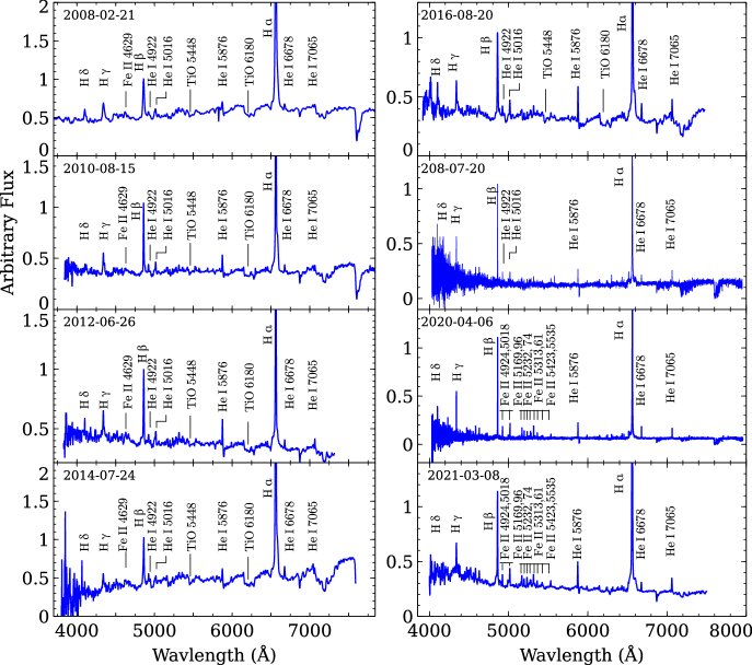
Figure 1: Dereddened spectra of Rs Oph, illustrating the spectroscopic evolution from days +0.99 to +14.91 in the upper panel and from days +17.97 to +25.84 in the lower panel. For the sake of clarity, the spectra are offset by the amount indicated on the left side of the figure. The ordinate scale is logarithmic to emphasise the visibility of weaker features relative to the emission feature of H $\alpha$. ’atm’ stands for atmospheric absorption seen at around 6876 Å, which appeared in all spectra at decreasing strengths.

The observed spectra display strong and broad emission lines attributed to hydrogen, helium, and iron, but the broadness of the lines noticed decreasing with time. The strong emission features noticed in the spectrum observed on 2008 February 22 are a result of recombination lines such as Balmer lines (from H $\alpha$ to H 8) and He I (4922, 5016, 5876 6678, and 7065 Å) lines. However, the presence of some Fe ii lines is also expected, either independently or blended, such as Fe ii (4233, 4491, 4584, 4924, 5018 Å). The absence of higher ionization lines can be accounted for by the absorption and softening caused by the reradiation of all direct photons from the accretion disc.

The strong TiO absorption features at 5448 and 6180 Å  are caused by the secondary. The Fe ii emission lines are a product of illumination from a high-density inner region of the disc undergoing photoionization. The quiescence phase of Rs Oph starts from $\sim$ 250 d, as a clear signatures of resumption of accreting matter and TiO  molecules detected at various wavelengths such as 4762, 5448, 5598, 5629 and 6159 Å  (Worters et al., 2007, 2008; Mondal et al., 2018).

The emission line profiles of the strongest four Balmer lines are depicted in the two panels of Fig. 2. The left column comprises the profiles of the H $\alpha$ and H $\beta$ lines, while the right column encompasses the profiles of the H $\gamma$ and H $\delta$ lines. The figure encompasses eight days’ worth of profiles for each line. Of these, the profiles from 2018 and 2020, acquired through a high-resolution telescope, distinctly exhibit a central double-peaked component feature. This feature, previously observed in prior outbursts (Brandi et al., 2009; Zamanov, 2011; Worters & Rushton, 2014), is notably conspicuous. The presence of a central, robust absorption feature in H $\alpha$ is mirrored in H $\beta$, suggesting a common origin for both lines.

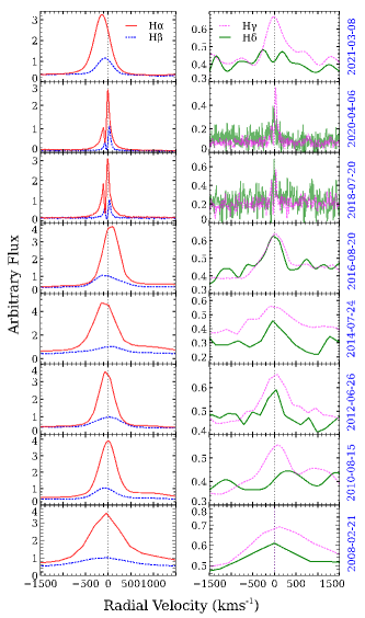
Figure 2: Plot of H $\alpha$, H $\beta$, H $\gamma$, and H $\delta$ emission line profiles of RS Oph during the quiescence phase happened between the 2006 and 2021 eruption. The dates presented in the left column also correspond to the respective right column in the same row. Similarly, the line labels presented at the top of each column also correspond to all rows below. The legends on the top panels of each column apply to all the panels below, and the dates provided on the right side of the second column serve as labels for the corresponding rows in the left column.

These profiles reveal an H $\alpha$ line structure akin to that observed during the quiescent stage of a preceding nova outburst (Brandi et al., 2009; Zamanov, 2011). The full width at half maximum (FWHM) of the H $\alpha$ line ranges from approximately 300 to 750 km/s, indicating increased strength compared to the quiescent stage of the nova in 1985. Specifically, the broad component of H $\alpha$ exhibits a FWHM of 747 km/s.

The H $\alpha$ line displays subtle positional shifts toward either the blue or red side, attributed to the orbital motion of the system. A similar phenomenon was observed in nova V3890 Sgr (Zemko et al., 2018). Comparable shifts in central position are noted in other Balmer lines (H $\beta$, H $\gamma$, and H $\delta$), albeit to a lesser extent in most cases.

The evolution of quiescence spectra of Rs Oph from day 740 to 5504, counted from 2006 Feb. 12.83 UT (which is considered as the outburst date ($t=0$)) is described here in Fig. 2 . The spectra cover the region from 4000 to 8000 Å. The prominent emission lines are marked in the figure. Strong emission patterns from the illuminated accretion disk that surrounds the WD, which is also the source of the strong blue continuum, are seen in the spectra. In general in all the quiescence phase, there was the appearance of strong and broad emission lines of hydrogen, helium and iron lines. The emission lines seen in these observed quiescence phase spectra are broad because of expanded discs (Anupama & Prabhu, 1989). Intense optical Fe II emission lines originate from a well-illuminated (photoionized) inner region of the disk with high density. As the disk accrues additional matter, these lines diminish, as noted by Bode & Evans (2008). The spectra also exhibit distinct absorption characteristics within the continuum, indicating the presence of cool secondaries and providing insights into the properties of these secondary components. Due to the cold secondaries, the spectra also exhibit noticeable continuous absorption features and expose the secondaries’ characteristics.

The spectrum captured on the day 740 (2008 Feb. 22.9 UT), shows prominent emission lines of H  (Balmer lines), He i ($\lambda$4922, $\lambda$5016, $\lambda$5876, $\lambda$6678, and $\lambda$7065 )Å, and O i $\lambda$ 8444Å together with significant secondary-contributed TiO  absorption features at 5448 and 6180 Å.

The most noticeable characteristic observed in the emission lines of the spectra considered in this study is a decrease in the width of Balmer lines over time (see Fig. 2). Among the spectra presented in Fig. 1, the maximum FWHM values for H $\alpha$ and H $\beta$ are 1055.9  km s^-1and 1034.89  km s^-1, respectively. Both of these values are obtained from the spectra observed on February 21, 2008. On the contrary the minimum FWHM is found to be 203.87  km s^-1.

4 Photoionization Model Analysis

We used the 2023 released version of the cloudy code (C23); Chatzikos et al. (2023) to model the spectra of nova RS Oph during its quiescent phase following the 2006 outburst. cloudy has been effectively applied to study novae including during the quiescent stage of a nova (Das & Mondal, 2015; Mondal et al., 2018; Pavana et al., 2019; Mondal et al., 2020). cloudy simulates the physical conditions of non-equilibrium gas clouds exposed to an external radiation field by using detailed microphysics. It predicts the emission-line spectrum based on assumptions about the gas’s physical conditions (ionisation, density, temperature, and chemical composition). The photoionization code cloudy uses a set of input parameters to compute the ionization, thermal and chemical state of a non-equilibrium gas cloud, illuminated by a central source, and it predicts the resulting spectra. The input parameters include the temperature (T) in Kelvins and luminosity (L) in  erg s^-1 of the central ionising source, hydrogen number density ($n$) in cm^-3, filling factor, covering factor, elemental abundances, and inner and outer radii (cm) of the surrounding ejecta. To generate synthetic model spectra, we incorporated all of these input parameters in our model along with the abundances of only those elements whose emission lines are observed in the spectra, while other elements are kept at their solar values from (Grevesse et al., 2010). In cloudy hydrogen density and filling factor varies radial as $n(r)=n(r_{o})(r/r_{o})^{\alpha}~{}\text{cm}^{-3}$ and $f(r)=f(r_{o})(r/r_{o})^{\beta}$, respectively, where $\alpha$ and $\beta$ are the exponents of the power laws, and $r_{0}$ is the inner radius. The density of the shell is controlled by a hydrogen density parameter with a power-law density profile and an exponent of -2 because it provides a steady mass per unit volume throughout the model disk ($\dot{\textrm{M}}=$ const). The ratio of the filled to vacuum volumes in the ejecta are set to 0.1, which is the value used in other recent Cloudy studies (Das & Mondal, 2015; Mondal et al., 2018, 2020).

The goodness of our model fit is estimated from the $\chi^{2}$ and $\chi_{red}^{2}$ of the model; using $\chi^{2}=\sum_{i=1}^{n}\frac{(M_{i}-O_{i})^{2}}{\sigma^{2}}$, and $\chi_{red}^{2}=\frac{\chi^{2}}{\nu}$ respectively, where $O_{i}$ and $M_{i}$ are the ratios of observed and modelled line fluxes to the H $\beta$ line flux, respectively, $\sigma_{i}$ is the error in the observed flux ratio, $\nu$ is the degrees of freedom given by $n-n_{p}$, n is the number of observed lines, and $n_{p}$ is the number of free parameters.An ideal model has a $\chi^{2}\approx\nu$ (Schwarz et al., 2001). Thus, the $\chi^{2}_{red}$ value of a model has to be low (typically in the range of 1-2) in order to be considered acceptable and well fitted. Normally, $\sigma$ ranges from 10 to 30 percent, depending on how strong it is relative to the continuum and whether it can blend with other lines in the spectrum (Helton et al., 2010).

5 Model Results

In this study, we modeled a total of seven spectra, offering broader spectral coverage ($\sim$ 3900 to $\sim$ 7500 Å ) and featuring a greater number of emission lines ($\sim$ 12 to 18 lines). These spectra span approximately twelve years (2008-2020), representing the duration when the nova was in the quiescent stage. The seven epochs were chosen with the aim of sampling the entire duration at roughly regular intervals for the sake of completeness, considering the availability of ideal spectra as well. The chosen seven epochs are Epoch 1 (2008-Feb-22), 2 (2010-Aug-15), 3 (2012-Jun-26), 4 (2014-Jul-24), 5 (2016-Aug-20), 6 (2018-Jul-20), and 7 (2020-Apr-2020); corresponding to days 740, 1645, 2326, 3085, 3843, 4542, and 5168, respectively. Among these seven epochs, the first five were modeled with one component, whereas the remaining two used two components of density and temperature.

To model the quiescent phase spectra of RS Oph, we developed a three-part model, consisting of the white dwarf (WD), the accretion disk formed on the WD’s surface, and the secondary star that feeds material to the accretion disk. The absorption features seen in the observed spectrum are a result of the secondary star. Various research results have showed the secondary of nova Rs Oph could be M0/M2III type (Scott et al., 1994; Anupama & Mikołajewska, 1999; Mondal et al., 2020). Therefore in this study we added the spectrum of the M2III-type giant to the modelled spectrum and found that it fits well with the absorption features. Only the model spectrum generated from the disk added with the black-body radiation from the WD was sufficient to produce the emission lines.

Initially, during the early years of the quiescent phase (from 2008-2016), we employed a one-component density profile across the radial distance of the accretion disk. However, as the nova approached the 2021 outburst (e.g in 2018 and 2020), the accretion disk expanded significantly, leading to the emergence of diverse spectral lines. To account for this, we divided the accretion disk into two components (see Fig. 3) with distinct density and temperature profiles and we added them to match the emission features by multiplying with the corresponding covering factors. We considered a small changes in temperature we assumed the luminosity won’t vary much as a result we didn’t change the luminosity. The inner region, characterized by higher density and temperature, was responsible for the generation of various iron lines observed in the spectrum, while the helium lines primarily originated from the same region. The Balmer lines, on the other hand, were produced by both components (Habtie et al., 2024; Pandey et al., 2022).

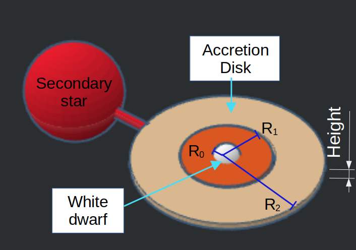
Figure 3: Schematic diagram of a nova system at the quiescence stage. The accretion disk is assumed to be cylindrical in shape and has two components of density and temperature. The symbols $R_{0}$, $R_{1}$, and $R_{2}$ represent the radius of the white dwarf (inner radius of the inner disk component), the outer radius of the inner disk component (the inner radius of the outer disk component), and the outer radius of the outer disk component, respectively.

To minimize the number of free parameters, the density power, filling factor, and inner and outer radii are held constant during the iterative process of fitting the observations. The hydrogen density, underlying luminosity, and effective blackbody temperature are allowed to vary. In addition, only the abundances of elements with observed lines are allowed to vary. All others are either set fully off or fixed at their solar values.

The inner and outermost radii of the accretion disc are calculated to be $R_{\text{in}}=10^{8.85}$ cm and $R_{\text{out}}=10^{13}$ cm. These radii are determined in the following ways:

1. To estimate the inner radius, we applied a rule by (Paczynski, 1977), which states that for a mass of $1M_{\odot}$, the inner radius is $10^{8.9}$ cm. By incorporating these values into the known relationship of radius and masses of the white dwarf (i.e., $M_{\text{WD}}^{(1/3)}R_{\text{WD}}$ = constant) (Gehrz et al., 1998), and applying it for the case of RS Oph, we found the inner radius of the accretion disk to be approximately $10^{8.85}$ cm.

2. To estimate the maximum possible radius of the accretion disk, we used the relation $R_{\text{A.disk}}(\text{max})/a=0.60/(1+q)$, where $a$ and $q$ represent the separation and ratio between the primary and secondary stars, respectively (Paczynski, 1977; Lasota et al., 2008; Sun et al., 2023). For the case of the secondary star being an M2III type star, whose mass ranges from 0.68 to $0.8M_{\odot}$ (Mikołajewska & Shara, 2017), we took the average of the lowest and highest possible masses of the secondary, which is $0.74M_{\odot}$, for better accuracy. Using Kepler’s third law and substituting the mentioned values along with the orbital period of 453.6 days (Brandi et al., 2009), we obtained the separation ($a$) to be $2.217\times 10^{11}$ m. We also obtained the value ratio ($q$) to be $q=0.54$. Finally, the maximum accretion disk radius of RS Oph was calculated to be $8.637\times 10^{12}$ cm. However, for the sake of simplicity, we used $10^{13}$ cm for our modeling.

As our model comprises about seven epochs, the outer radii of individual epochs, excluding the last epoch, were decided according to the fitting level of the synthetic spectrum with the observed one. While not solely relying on the fitting, we assumed that the accretion disk size grew linearly with time. With this assumption in mind, we used the best-fitting level to determine the exact values of radii.

From the best-fitting model, we have obtained values for various physical and chemical parameters of the RS Oph system during its quiescent phase. These parameters include the temperature and luminosity of the source, hydrogen number density, dimensions, and composition of the accretion disk formed on the surface of the white dwarf (see Table 2). In Fig. 4, we present the best-fitting synthetic spectra overlaid on the observed spectra of RS Oph on seven distinct days, covering a roughly estimated range of two years. Both the modeled and observed spectra are normalized to the line flux of H $\beta$, and the observed spectra are dereddened by E(B-V)=0.73 (Snijders, 1987; Pandey et al., 2022).

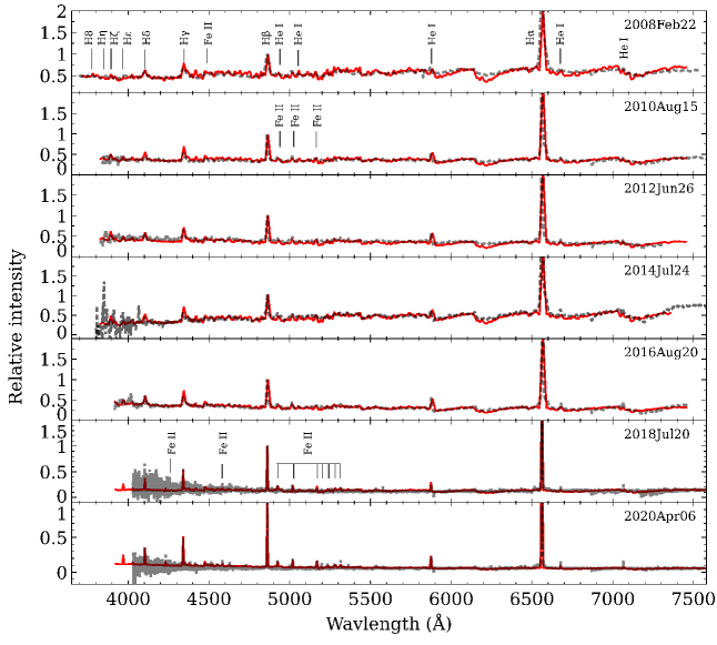
Figure 4: Observed spectra during the quiescence phase of novae RS Oph (grey dashed line) alongside model-generated spectra (red solid line). Dates of observation for each epoch are indicated on the right side of each panel. Spectra have been normalized with respect to the H $\beta$ line. Prominent emission lines are highlighted in the figure. For more details, please refer to Section 5.

We computed a set of synthetic spectra by simultaneously varying all the aforementioned input parameters in smaller increments across a broad sample space. The temperature ranged from $10^{3.5}$ to $10^{6}$ K, luminosity varied between $10^{37}$ and $10^{38}$  erg s^-1, and ejecta density spanned $10^{6.5}$ to $10^{13}\text{cm}^{-3}$, concurrently with the elemental abundances. Multiple test models were iterated across all epochs before arriving at the final model. Initial visual examinations were conducted, and models that did not align with the observed spectrum were discarded. To assess the fit quality, we calculated the $\chi^{2}$ and $\chi^{2}_{\text{red}}$ values of the model, as discussed in section 4. A comparison of the relative fluxes for the best-fitting model-predicted lines and the observed lines during the early phase is presented in Table 3, along with the corresponding $\chi^{2}$. For the calculation of $\chi^{2}$ values, we selected emission lines that appear in both observational and modeled spectra. To determine the line fluxes in individual emission lines, interactive flux measurements were performed by fitting Gaussians using the splot task of the onedspec package in IRAF. To mitigate inaccuracies related to flux calibration among various epochs, flux ratios of observed and modeled emission lines relative to H $\beta$ were calculated.

5.1 Temperature, Luminosity and Density

From the first epoch (2008) to the fifth (2016), we applied a one-component model. The temperature and luminosity of the source increased from $1.047\times 10^{4}$ K and $1\times 10^{29}$  erg s^-1to $1.202\times 10^{4}$ K and $1\times 10^{30}$  erg s^-1, respectively. Similarly, the density and outer radius increased from $3.16\times 10^{7}$ $cm^{-3}$ and $3.20\times 10^{9}$ cm to $6.309\times 10^{8}$ $cm^{-3}$ and $1.584\times 10^{11}$ cm, respectively. For the sixth and seventh epochs, a two-component model was employed, where the hydrogen number density and temperature varied. We opted not to vary the luminosity, as we observed that the fitting process was somewhat insensitive to small variations in luminosity. Similar to the patterns observed in the previous epochs, the temperature, luminosity, and density continued to increase in these cases as well (see the values in columns 7-10 of Table 2).

5.2 Elemental composition

In all of the epochs we modeled and analyzed, we have detected the presence of He i and Fe ii, in addition to the ubiquitous Balmer lines typical of such novae. Our modeling revealed a significant decrease in the abundance of helium throughout the quiescent stage of the nova RS Oph. For example, the He /He $\odot$ ratio was reported as 2.4 in the first epoch but decreased to the solar value for epochs 6 and 7. In the initial three epochs (2008, 2010, and 2012), Fe  exhibited subsolar abundances in the accretion disk. However, from the fourth epoch (2014) onward, it showed a considerable increase, appearing overabundant. The Fe /Fe $\odot$ ratio in the first and last epochs was obtained as 0.5 and 2.5, respectively. This indicates a significant enhancement in iron abundance as the nova approaches the upcoming outburst, possibly due to the secondary star continuously providing a substantial amount of cold iron through the inner Lagrange point (see rows 7 and 8 of Table 2, counting from bottom to top). The possible reason for this enhanced abundance of iron over the solar value could be because the companion star had evolved beyond the main-sequence level (Bode & Evans, 2008)

The helium abundance across all epochs was determined by fitting the prominent He i lines (4026, 4471, 4922, 5016, 5048, 5876, 7065 Å). Most likely, the majority of these lines originated from the inner portion of the accretion disk, which is denser than the outer portion. During modeling, we clearly observed that a higher density needed to be set to achieve a better fit over these lines. Moreover, the two-component model for the last two epochs clearly illustrated this by showing that most of the mentioned helium lines originated from the inner disk component. This is consistent with Zemko et al. (2018), for the case 2011 and 2012. Some helium lines are blended with other lines, such as He i 4922 and 5016, making it difficult to conclusively determine the absolute generating regions of helium in the accretion disk. This observation of helium generated from higher density regions is also common in other nova systems (e.g., V1674 Her (Habtie et al., 2024; Pandey et al., 2022)).

The iron abundance for each epoch was determined by fitting specific lines from Fe ii (4233, 4415, 4491, 4584, 4629, 4924, 5018, 5169, 5232, 5276, 5361, and 5538 Å). These lines predominantly originated from lower-density regions of the disk, with some contributions observed from higher-density areas. This observation is consistent with Banerjee et al. (2009), who pointed out that the Fe II emission, which seems to be favored by high-density conditions, originates from a region associated with the contact discontinuity. Fe ii signifies a low ionization stage, suggesting its origin in a zone characterized by low kinetic temperature (a similar reasoning applies to the presence of neutral o i lines, indicating their coexistence with Fe ii).

5.3 Accretion mass & rate

The ejected mass within the model disk could be calculated using the following equation, (Schwarz et al., 2001):

$$M_{\text{disc}}=n(r_{0})f(r_{0})\int_{R_{\text{in}}}^{R_{\text{out}}}\left(\frac{r}{r_{0}}\right)^{\alpha+\beta}2\pi rdr\int_{0}^{h}dz,$$ (1)

where $n(r_{0})$ represents the hydrogen density ($\text{cm}^{-3}$) and $f(r_{0})$ stands for the filling factor at the inner radius of the shell ($r_{0}$). The exponents $\alpha$ and $\beta$ correspond to the power laws. The values for density, filling factor, $\alpha$, and $\beta$ are directly adopted from the best-fitting cloudy model parameters (refer to Table 2). The estimation of the total ejected shell mass involved multiplying the mass in both density components (clump and diffuse) with their corresponding covering factors and subsequently adding them together. Consequently, the ejected hydrogen shell masses for epochs 1, 2, 3, 4, 5, 6, and 7 are estimated to be: $8.94\times 10^{-16}M_{\odot}$, $5.39\times 10^{-15}M_{\odot}$, $2.52\times 10^{-14}M_{\odot}$, $4.033\times 10^{-14}M_{\odot}$, $8.019\times 10^{-14}M_{\odot}$, $3.646\times 10^{-8}M_{\odot}$, and $1.63\times 10^{-7}M_{\odot}$ , respectively. Fig. 5 illustrates the growth of the accretion disk over time in terms of both mass and radius.

According to Worters et al. (2007); Mondal et al. (2018), the presence of an accretion disk was detected in April 2007. Therefore, we assumed that the mass estimated from the first epoch in our model represents the amount accreted from that day. As a result, we considered our quiescent phase modeling of RS Oph spectra to cover a period of 13 years. Utilizing the accreted masses estimated from the best-fit parameters of our photoionization model, we calculated a mean accretion rate of approximately $1.254\times 10^{-8}M_{\odot}$ $\text{yr}^{-1}$. Remarkably, this value is in excellent agreement with the previous estimates independently made by Hachisu & Kato (2000) and Nelson et al. (2011), both of which were approximately $1.2\times 10^{-8}M_{\odot}$ $\text{yr}^{-1}$.

The critical accretion disk mass necessary for initiating thermonuclear runaway (TNR) can be estimated by considering the critical pressure in the inner layers of the disk ($10^{15}$ $Ncm^{-2}$) (Truran & Livio, 1986), as expressed by the formula:

$$M_{\text{acc}}\approx\dfrac{4\pi R_{\text{WD}}^{4}}{GM_{\text{WD}}}P_{\text{crit}}$$ (2)

where $G=6.67\times 10^{-11}$ $Nm^{2}kg^{-2}$, and $R_{\text{WD}}$ and $M_{\text{WD}}$ represent the radius and mass of the white dwarf (WD). Additionally, we determine the WD radius using the Nauenberg (1972) mass-radius approximation given in Yaron et al. (2005):

$$R_{\text{WD}}\approx 1.12\times 10^{-2}\left[\left(\dfrac{M_{\text{WD}}}{M_{ch}}\right)^{-2/3}-\left(\dfrac{M_{\text{WD}}}{M_{ch}}\right)^{2/3}\right]^{1/2}R_{\odot},$$ (3)

We obtained WD radii ($R_{\text{WD}}$) of approximately $1.72$ and $1.159\times 10^{8}$ cm, respectively. The critical mass required to be accreted onto the WD was then computed using equation 2, resulting in values of $3.066\times 10^{-7}M_{\odot}$ and $6.27\times 10^{-8}M_{\odot}$, respectively.

We promptly dismissed the result derived from a mass of 1.377$M_{\odot}$ as it proves incompatible with our model. This outcome implies that the critical accreted mass is lower than the mass estimated by our model approximately 15 months before the outburst, a scenario deemed implausible. Consequently, we exclusively selected the mass of 1.35$M_{\odot}$ for subsequent analysis.

In the context of the temporal span extending from the initial reported onset of accretion in April 2007 (Worters et al., 2007; Mondal et al., 2018) to the subsequent outburst in August 2021, spanning approximately 14 years, we calculated the mean accretion rate for white dwarf masses of 1.35$M_{\odot}$ to be $2.19\times 10^{-8}M_{\odot}\text{yr}^{-1}$. This calculated value exhibited reasonable alignment with the accretion rate determined through our model, which was $1.254\times 10^{-8}M_{\odot}$ $\text{yr}^{-1}$.

Upon scrutinizing the acquired results, a noteworthy observation emerges: the accretion rate derived from our model exhibits closer proximity to the accretion rate associated with a WD mass of $1.35M_{\odot}$. This proximity serves as an indicative insight, suggesting that the true mass of the white dwarf (WD) in the system Rs Oph may approximate $\sim 1.35M_{\odot}$ but be less than $1.377M_{\odot}$ as it provides us with an invalid output.

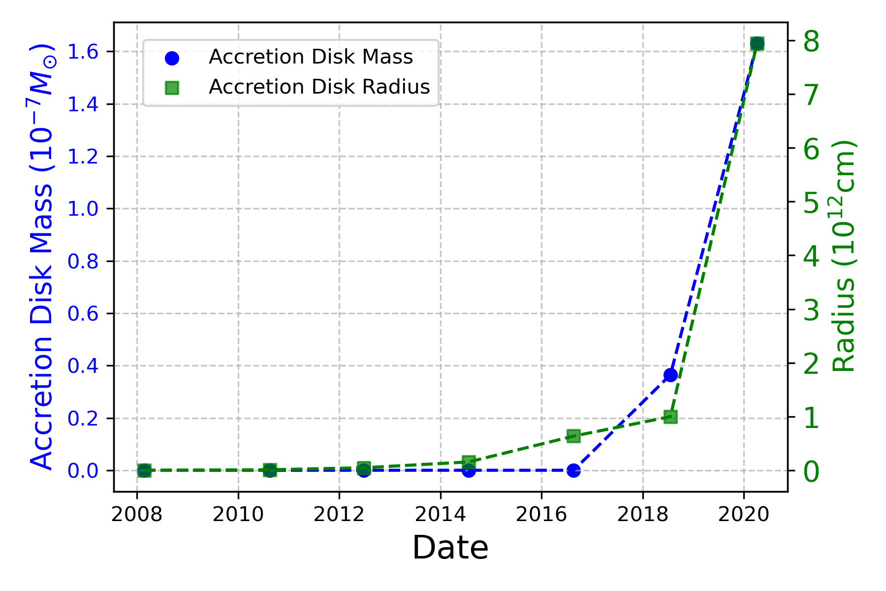
Figure 5: Temporal Evolution of Accretion Disk Mass and Radius: This plot showcases the dynamic interplay between accretion disk mass and radius over time, providing a comprehensive view of the system’s evolution.

6 Discussion

The paper explores the optical spectral evolution of Rs Oph during its quiescent phase, spanning from nearly the onset of the quiescent phase following the 2006 outburst to the 2021 outburst. Despite Rs Oph being well-studied, the quiescent stage of the nova remains largely unexplored. The observed quiescent phase spectra considered in this study bear a strong resemblance to some of the spectra observed at the same phase following the 1985 outburst. For instance, the $1987^{th}$ spectrum provided by Anupama & Prabhu (1989) shows a striking similarity to that of the $2008^{th}$ spectrum of the 2006 outburst. However, the spectrum collected in 1988 exhibits a considerable mismatch with any of the spectra considered in this study. Notably, in the 1988 spectrum, H $\beta$ appears with a line strength comparable to other non-Balmer lines, a situation that doesn’t occur in any of the spectra considered in this study. This phase, potentially resembling previous outbursts, exhibits many variations in the physical conditions at different epochs, providing valuable insights into the system. The study benefits from comprehensive coverage, enabling the investigation of distinct ionization lines and the evolution of line profiles, shedding light on the nuanced characteristics of Rs Oph during its quiescent stage.

Using photoionization cloudy modeling, we estimated various parameters of the accretion disk formed on the surface of the white dwarf, with all values provided in Table 2. In the initial couple of years, starting from 2008, we observed a relatively cool and less luminous system, possibly indicating that it had fully entered the quiescent phase with minimal matter accretion at that moment. Over time, both the temperature and luminosity increased. Similarly, due to the limited amount of matter accreted during that period, the hydrogen number density appeared low initially but evolved rapidly. The dimensions of the accretion disk also increased monotonically in the radial component of a cylindrical geometry.

According to our model, during the initial four years from 2008, the abundance of iron was significantly lower than the solar value. This discrepancy could be attributed to the limited quantity of accreted matter, resulting in an insufficient amount of iron reaching the disk. The model predicts that the iron abundance surpasses the solar value from 2014 onward, increasing rapidly. This trend aligns with the notion that iron originates from the secondary star.

From the best-fit parameters obtained through our photoionization model, we determined the mass of the accretion disk at seven different epochs during the quiescent stage from 2008 to 2020. In the first epoch, as anticipated, the white dwarf (WD) accreted a relatively small mass of $8.94\times 10^{-16}M_{\odot}$. This observation aligns with expectations, considering that the nova had transitioned to the quiescent phase in April 2007 (Mondal et al., 2018), less than a year before the first epoch. The accretion mass showed a gradual increase during Epochs 2, 3, 4, and 5, measuring $5.39\times 10^{-15}M_{\odot}$, $2.52\times 10^{-14}M_{\odot}$, $4.033\times 10^{-14}M_{\odot}$, and $8.019\times 10^{-14}M_{\odot}$, respectively. In these epochs, the accretion mass exhibited a relatively slower growth rate. However, during Epochs 6 and 7, the accretion disk’s mass increased more rapidly, reaching $3.646\times 10^{-8}M_{\odot}$ and $1.63\times 10^{-7}M_{\odot}$, respectively. The observed acceleration of accretion rate can be attributed to the overall increase in the mass of the system (white dwarf and accretion disk) caused by the accumulation of matter on the white dwarf’s surface. This results in a more efficient extraction of material from the secondary star’s surface, utilizing the enhanced gravitational pull.

Employing Equation 2, we computed the critical mass of the accretion disk essential for initiating thermonuclear runaway (TNR) for a specific white dwarf (WD) mass (1.35$M_{\odot}$) to be $2.32\times 10^{-7}M_{\odot}$. According to our model, by Epoch 7 (2020), the accreted mass on the WD had reached approximately $1.63\times 10^{-7}M_{\odot}$, resulting in a deficit of $1.436\times 10^{-7}M_{\odot}$ to reach the critical mass limit. We observed that only 53% of the critical mass had been accreted by February 22, 2020, with the remaining substantial mass (approximately 47%) accreted onto the white dwarf in the subsequent 15 months.

If we commence the analysis from 2018, where the model estimated the accreted mass up to July 20, 2018, as $3.646\times 10^{-8}M_{\odot}$, the deficit to reach the critical mass is approximately $2.7\times 10^{-7}M_{\odot}$; representing about 88% of the critical mass required to initiate the TNR processes.

This observation highlights that the accretion rate in the final years is significantly higher than in the preceding years, attributed to the increased gravitational attraction resulting from the mass already deposited onto the WD.

Table 2: Best Fit cloudy Model Parameters for Quiescent Stages of RS Oph: 2006 to 2021 Outburst.

Parameters	Values
	Epoch 1	Epoch 2	Epoch 3	Epoch 4	Epoch5	Epoch6		Epoch7
						diskin	diskout	diskin	diskout
Black Body Temperature ($\times 10^{4}$K)	1.047	1.072	1.096	1.148	1.202	1.698	1.096	1.778	1.122
Luminosity ($\times 10^{30}$  erg s-1)	0.100	0.158	0.316	0.501	1.000	3.981	3.981	7.943	7.943
Hydrogen density ($\times 10^{10}\text{cm}^{-3}$)	0.316	1.000	3.162	3.981	6.309	10.00	1.000	31.62	3.162
$\alpha$	-2.000	-2.000	-2.000	-2.000	-2.000	-2.000	-2.000	-2.000	-2.000
Inner radius ($\times 10^{9}\text{cm}$)a	0.708	0.708	0.708	0.708	0.708	0.708	31.62	0.708	31.622
Outer radius ($\times 10^{11}\text{cm}$)a	0.032	0.126	0.50	1.584	6.309	0.316	10.00	0.316	100.0
Filling Factora	0.100	0.100	0.100	0.100	0.100	0.100	0.100	0.100	0.100
$\beta$a	0.000	0.000	0.000	0.000	0.000	0.000	0.000	0.000	0.000
Covering factor (AD:BB:SE)	45.5:15.5:39.0	62.5:15.5:22.0	63.0:17.5:19.5	59.0:10.0:33.0	65.0:16.0:17.0	42.0:3.0:8.0	44.0:3.0:8.0	43.0:2.0:3.0	49.0:3.0:3.0
He /He ☉b	2.400	1.800	2.100	2.100	2.100	1.100	1.100	1.000	1.000
Fe /Fe ☉b	0.500	0.500	0.800	1.900	2.100	2.400	2.400	2.500	2.500
Ejected matter mass ($\times 10^{-5}~{}M_{\sun}$)	-	-	-	-	-	-		-
Number of lines	22.0	17.0	20.0	18.0	19.0	19		19
Number of free parameters	6.000	6.000	6.000	6.000	6.000	6.000		6.000
Degrees of freedom	16.00	11.00	14.00	12.00	13.00	13		13
$\chi_{\text{tot}}^{2}$	28.314	16.203	27.834	16.652	17.8561	13.263		14.471
$\chi_{\text{red}}^{2}$	1.771	1.473	1.988	1.388	1.374	1.020		1.113

Note: ^a stands for the quantity is not considered as a free parameter.
       ^b Abundances are given in logarithmic scale, relative to the solar value. Due to an unprecedented mismatch between the model and observed spectra, we have excluded the presence of certain elements in our
        model spectra, including Carbon, Oxygen, Nitrogen, and Neon.

Table 3: Observed and best-fit cloudy model line flux values for quiescent phase epochs of Rs Oph.

Line		Epoch 1 (2008Feb22)			Epoch 2 (2010Aug15)			Epoch 3 (2012Jun26)			Epoch 4 (2014Jul24)			Epoch 5 (2016Aug20)			Epoch 6 (2018Jul20)			Epoch (2020Apr06)
ID	$\lambda$ (Å)	mod.	Obs.	$\chi^{2}$	mod.	Obs.	$\chi^{2}$	mod.	Obs.	$\chi^{2}$	mod.	Obs.	$\chi^{2}$	mod.	Obs.	$\chi^{2}$	mod.	Obs.	$\chi^{2}$	mod.	Obs.	$\chi^{2}$
H 8	3770	0.332	0.271	0.365	-	-	-	-	-	-	-	-	-	-	-	-	-	-	-	-	-	-
H $\eta$	3835	0.149	0.185	0.132	-	-	-	-	-	-	-	-	-	-	-	-	-	-	-	-	-	-
H $\zeta$	3889	0.165	0.125	0.164	0.417	0.331	2.945	0.324	0.287	0.095	0.330	0.172	1.482	-	-	-	-	-	-	-	-	-
H $\epsilon$	3970	0.086	0.188	1.051	0.288	0.248	0.655	0.296	0.441	1.447	0.167	0.336	1.688	0.162	0.066	0.416	-	-	-	-	-	-
He i	4026	-	-	-	-	-	-	0.257	0.376	0.971	0.229	0.111	0.827	0.110	0.134	0.026	-	-	-	-	-	-
H $\delta$	4101	0.404	0.355	0.244	0.530	0.424	4.571	0.372	0.277	0.633	0.368	0.210	1.477	0.356	0.470	0.577	0.227	0.202	0.081	0.209	0.232	0.102
Fe ii	4233	0.099	0.088	0.013	0.196	0.220	0.222	0.259	0.242	0.020	0.083	0.087	0.001	0.097	0.116	0.016	0.068	0.073	0.003	0.056	0.095	0.307
H $\gamma$	4340	0.832	0.743	0.792	0.666	0.688	0.197	0.658	0.869	3.076	0.631	0.661	0.054	0.615	0.533	0.295	0.456	0.284	3.652	0.431	0.204	10.51
Fe ii	4415	0.286	0.109	3.130	-	-	-	0.391	0.412	0.030	0.260	0.303	0.106	0.120	0.082	0.066	0.118	0.041	0.742	0.059	0.030	0.171
He i	4471	-	-	-	-	-	-	-	-	-	-	-	-	0.238	0.107	0.761	0.149	0.037	1.534	0.094	0.068	0.138
Fe ii	4491	0.542	0.237	9.288	-	-	-	-	-	-	-	-	-	-	-	-	-	-	-	-	-	-
Fe ii	4584	0.406	0.318	0.788	0.378	0.351	0.277	0.324	0.511	2.143	-	-	-	0.091	0.162	0.229	0.105	0.107	0.00037	0.055	0.059	0.003
Fe ii	4629	0.652	0.527	1.561	-	-	-	0.468	0.765	6.143	-	-	-	0.115	0.249	0.795	0.153	0.026	1.984	0.055	0.071	0.052
H $\beta$	4861	1.000	1.000	0.000	1.000	1.000	0.000	1.000	1.000	0.000	1.000	1.000	0.000	1.000	1.000	0.000	1.000	1.000	0.000	1.000	1.000	0.000
He i	4922	0.395	0.591	3.850	0.281	0.336	1.229	0.327	0.459	1.206	0.392	0.458	0.257	0.178	0.283	0.492	-	-	-	-	-	-
Fe ii	4924	-	-	-	-	-	-	-	-	-	-	-	-	-	-	-	0.277	0.111	3.385	0.091	0.099	0.016
He i	5016	0.326	0.515	3.587	0.289	0.205	2.845	0.335	0.547	3.129	0.374	0.651	4.528	0.163	0.311	0.979	-	-	-	-	-	-
Fe ii	5018	-	-	-	-	-	-	-	-	-	-	-	-	-	-	-	0.155	0.125	0.10754	0.121	0.124	0.003
He i	5048	0.441	0.349	0.835	-	-	-	-	-	-	-	-	-	0.105	0.272	1.243	-	-	-	-	-	-
Fe ii	5169	0.246	0.290	0.196	0.313	0.391	2.451	0.237	0.075	1.822	0.400	0.505	0.654	0.165	0.214	0.107	0.197	0.169	0.111	0.139	0.082	0.657
Fe ii	5232	0.337	0.356	0.035	0.289	0.227	1.516	0.201	0.355	1.647	0.315	0.463	1.302	0.121	0.116	0.001	0.142	0.111	0.115	0.036	0.061	0.117
Fe ii	5276	0.428	0.585	2.453	0.384	0.418	0.473	0.265	0.383	0.966	0.357	0.291	0.259	0.130	0.308	1.392	0.155	0.082	0.648	0.076	0.068	0.012
Fe ii	5361	0.463	0.785	10.346	0.404	0.268	7.391	0.271	0.468	2.696	0.474	0.616	1.195	-	-	-	0.134	0.072	0.473	0.067	0.061	0.009
Fe ii	5538	-	-	-	-	-	-	-	-	-	-	-	-	0.207	0.228	0.021	0.086	0.063	0.066	0.031	0.043	0.028
He i	5876	0.541	0.565	0.056	0.551	0.558	0.021	0.471	0.391	0.435	0.617	0.456	1.523	0.477	0.454	0.024	0.286	0.233	0.347	0.243	0.138	2.242
H $\alpha$	6563	-	-	-	3.499	3.376	6.087	-	-	-	-	-	-	3.368	3.839	9.871	-	-	-	-	-	-
He i	6678	0.727	0.730	0.001	0.365	0.348	0.114	0.162	0.252	0.573	0.373	0.458	0.430	0.172	0.151	0.022	0.104	0.105	0.000	0.073	0.064	0.01502
He i	7065	0.545	0.682	1.883	0.2815	0.325	0.764	0.157	0.264	0.802	0.331	0.452	0.869	0.127	0.236	0.523	0.111	0.097	0.027	0.049	0.070	0.094

7 Conclusions

In conclusion, our investigation of RS Oph during the quiescent phase between the 2006 and 2021 outbursts employed photoionization-based modeling and spectroscopic analysis to elucidate the accretion disk formation process, encompassing its composition, mass, and dimensions. The key findings are summarized as follows:

1. The spectra during the quiescent phase reveal distinctive low-ionization emission features, including hydrogen, helium, iron, and TiO absorption features originating from the cool secondary component.

2. Utilizing the CLOUDY photoionization code, we determined that the central ionizing sources exhibit temperatures in the range of $1.05-1.8~{}\times 10^{4}$ K and luminosities between $0.1-7.9~{}\times 10^{30}$  erg s^-1.

3. The abundance of He  displayed temporal variations, showing an overabundance from 2008 to 2016, returning to solar values by 2020. Meanwhile, Fe  appeared subsolar from 2008 to 2014 but became overabundant from 2006 onward.

4. The critical mass of the white dwarf (WD) has been calculated for WD masses of $1.35M_{\odot}$ and $1.377M_{\odot}$, resulting in values of $3.066\times 10^{-7}M_{\odot}$ and $6.27\times 10^{-8}M_{\odot}$, respectively. The latter result was excluded from consideration as it is already less than the accreted mass determined at our last epoch (February 22, 2020). This exclusion supports the conclusion that the mass of the WD likely falls within the range of $1.350M_{\odot}\leq M_{WD}<1.377M_{\odot}$.

5. The mean accretion rate, as calculated from the model, is approximately $1.254\times 10^{-8}M_{\odot}$ yr^-1. However, it is important to note that this value does not imply uniform accretion dynamics over time. About 47% of the critical mass was accreted in the last 15 months, and approximately 88% of the critical mass was accreted after July 20, 2018. This non-uniform accretion rate suggests a more rapid approach towards reaching the critical mass in the final years. This phenomenon could be attributed to the heightened gravitational pull resulting from previously accreted matter, influencing the accretion dynamics as the system approaches the critical mass limit.

Data Availability

The paper utilizes spectroscopic data obtained from three sources: the Astronomical Ring for Access to Spectroscopy Database (ARAS Database; Teyssier (2019)), Stony Brook/SMARTS Atlas of (mostly) Southern Novae ((Walter et al., 2012)), European Southern Observatory (ESO) (Pickles, 1998), and Astrosurf Recurrent Nova. These spectroscopic data were employed to analyse the spectral evolution of the system and for modeling purposes presented in Fig. 1 and  4.

Appendix A Some extra material

If you want to present additional material which would interrupt the flow of the main paper, it can be placed in an Appendix which appears after the list of references.

References

- Anupama (2008) Anupama G. C., 2008, in Evans A., Bode M. F., O’Brien T. J., Darnley M. J., eds, Astronomical Society of the Pacific Conference Series Vol. 401, RS Ophiuchi (2006) and the Recurrent Nova Phenomenon. p. 31
- Anupama & Mikołajewska (1999) Anupama G. C., Mikołajewska J., 1999, A&A, 344, 177
- Anupama & Prabhu (1989) Anupama G. C., Prabhu T. P., 1989, Journal of Astrophysics and Astronomy, 10, 237
- Azzollini et al. (2023) Azzollini A., Shore S. N., Kuin P., Page K. L., 2023, A&A, 674, A139
- Banerjee et al. (2009) Banerjee D. P. K., Das R. K., Ashok N. M., 2009, MNRAS, 399, 357
- Bode & Evans (2008) Bode M. F., Evans A., 2008, Classical Novae, 2 edn. Cambridge Astrophysics, Cambridge University Press, doi:10.1017/CBO9780511536168
- Booth et al. (2016) Booth R. A., Mohamed S., Podsiadlowski P., 2016, MNRAS, 457, 822
- Brandi et al. (2009) Brandi E., Quiroga C., Mikołajewska J., Ferrer O. E., García L. G., 2009, A&A, 497, 815
- Chatzikos et al. (2023) Chatzikos M., et al., 2023, Rev. Mex. Astron. Astrofis., 59, 327
- Das & Mondal (2015) Das R., Mondal A., 2015, New Astron., 39, 19
- Gehrz et al. (1998) Gehrz R. D., Truran J. W., Williams R. E., Starrfield S., 1998, PASP, 110, 3
- Grevesse et al. (2010) Grevesse N., Asplund M., Sauval A. J., Scott P., 2010, Ap&SS, 328, 179
- Habtie et al. (2024) Habtie G. R., Das R., Pandey R., Ashok N. M., Dubovsky P. A., 2024, MNRAS, 527, 1405
- Hachisu & Kato (2000) Hachisu I., Kato M., 2000, ApJ, 536, L93
- Hachisu et al. (2007) Hachisu I., Kato M., Luna G. J. M., 2007, ApJ, 659, L153
- Helton et al. (2010) Helton L. A., et al., 2010, AJ, 140, 1347
- Hjellming et al. (1986) Hjellming R. M., van Gorkom J. H., Taylor A. R., Sequist E. R., Padin S., Davis R. J., Bode M. F., 1986, ApJ, 305, L71
- Kato et al. (2008) Kato M., Hachisu I., Luna G. J. M., 2008, in Evans A., Bode M. F., O’Brien T. J., Darnley M. J., eds, Astronomical Society of the Pacific Conference Series Vol. 401, RS Ophiuchi (2006) and the Recurrent Nova Phenomenon. p. 308 (arXiv:0807.1251), doi:10.48550/arXiv.0807.1251
- Lasota et al. (2008) Lasota J. P., Dubus G., Kruk K., 2008, A&A, 486, 523
- Mikołajewska & Shara (2017) Mikołajewska J., Shara M. M., 2017, ApJ, 847, 99
- Mondal et al. (2018) Mondal A., Anupama G. C., Kamath U. S., Das R., Selvakumar G., Mondal S., 2018, MNRAS, 474, 4211
- Mondal et al. (2020) Mondal A., Das R., Anupama G. C., Mondal S., 2020, MNRAS, 492, 2326
- Munari & Tabacco (2022) Munari U., Tabacco F., 2022, Research Notes of the American Astronomical Society, 6, 103
- Nauenberg (1972) Nauenberg M., 1972, ApJ, 175, 417
- Nelson et al. (2011) Nelson T., Mukai K., Orio M., Luna G. J. M., Sokoloski J. L., 2011, ApJ, 737, 7
- Osborne et al. (2011) Osborne J. P., et al., 2011, ApJ, 727, 124
- Paczynski (1977) Paczynski B., 1977, ApJ, 216, 822
- Pandey et al. (2022) Pandey R., Habtie G. R., Bandyopadhyay R., Das R., Teyssier F., Guarro Fló J., 2022, MNRAS, 515, 4655
- Parthasarathy et al. (2007) Parthasarathy M., Branch D., Jeffery D. J., Baron E., 2007, New Astron. Rev., 51, 524
- Pavana et al. (2019) Pavana M., Anche R. M., Anupama G. C., Ramaprakash A. N., Selvakumar G., 2019, A&A, 622, A126
- Pickles (1998) Pickles A. J., 1998, PASP, 110, 863
- Schaefer (2004) Schaefer B. E., 2004, IAU Circ., 8396, 2
- Schaefer (2010) Schaefer B. E., 2010, ApJS, 187, 275
- Schwarz et al. (2001) Schwarz G. J., Shore S. N., Starrfield S., Hauschildt P. H., Della Valle M., Baron E., 2001, MNRAS, 320, 103
- Scott et al. (1994) Scott A. D., Rawlings J. M. C., Krautter J., Evans A., 1994, MNRAS, 268, 749
- Snijders (1987) Snijders M. A. J., 1987, Ap&SS, 130, 243
- Sun et al. (2023) Sun Q.-B., Qian S.-B., Zhu L.-Y., Liao W.-P., Zhao E.-G., Li F.-X., Shi X.-D., Li M.-Y., 2023, MNRAS, 526, 3730
- Teyssier (2019) Teyssier F., 2019, Contributions of the Astronomical Observatory Skalnate Pleso, 49, 217
- Truran & Livio (1986) Truran J. W., Livio M., 1986, ApJ, 308, 721
- Van Winckel et al. (1993) Van Winckel H., Duerbeck H. W., Schwarz H. E., 1993, A&AS, 102, 401
- Walker (1977) Walker A. R., 1977, MNRAS, 179, 587
- Walter et al. (2012) Walter F. M., Battisti A., Towers S. E., Bond H. E., Stringfellow G. S., 2012, PASP, 124, 1057
- Williams et al. (1994) Williams R. E., Phillips M. M., Hamuy M., 1994, ApJS, 90, 297
- Worters & Rushton (2014) Worters H. L., Rushton M. T., 2014, MNRAS, 442, 2637
- Worters et al. (2007) Worters H. L., Eyres S. P. S., Bromage G. E., Osborne J. P., 2007, MNRAS, 379, 1557
- Worters et al. (2008) Worters H. L., Eyres S. P. S., Bromage G. E., Osborne J. P., 2008, in Evans A., Bode M. F., O’Brien T. J., Darnley M. J., eds, Astronomical Society of the Pacific Conference Series Vol. 401, RS Ophiuchi (2006) and the Recurrent Nova Phenomenon. p. 223
- Yaron et al. (2005) Yaron O., Prialnik D., Shara M. M., Kovetz A., 2005, ApJ, 623, 398
- Zamanov (2011) Zamanov R. K., 2011, Bulgarian Astronomical Journal, 17, 59
- Zemko et al. (2018) Zemko P., et al., 2018, MNRAS, 480, 4489