Smart Flow Matching:
On The Theory of Flow Matching Algorithms with Applications

Abstract

The paper presents the exact formula for the vector field that minimizes the loss for the standard flow. This formula depends analytically on a given distribution $\rho_{0}$ and an unknown one $\rho_{1}$. Based on the presented formula, a new loss and algorithm for training a vector field model in the style of Conditional Flow Matching are provided. Our loss, in comparison to the standard Conditional Flow Matching approach, exhibits smaller variance when evaluated through Monte Carlo sampling methods. Numerical experiments on synthetic models and models on tabular data of large dimensions demonstrate better learning results with the use of the presented algorithm.

1 Introduction

In recent years, there has been a remarkable surge in Deep Learning, wherein the advancements have transitioned from purely neural networks to tackling differential equations. Notably, Diffusion Models (Sohl-Dickstein et al., 2015) have emerged as key players in this field. These models leverage the mathematics of diffusions, which are continuous-time stochastic processes, to model probability distributions. One key aspect of diffusion models is the ability to transform a simple initial distribution, usually a standard Gaussian distribution, into a target distribution via a sequence of transformations.

The Conditional Flow Matching (CFM) (Lipman et al., 2023) technique, which we focus on in our research, is a promising approach for constructing probability distributions using conditional probability paths, which is notably a robust and stable alternative for training Diffusion Models.

Further works have attempted to improve the convergence, quality or speed of CFM by using various heuristics. For example, in the works (Tong et al., 2023b, a; Liu et al., 2022) it was proposed to straighten the trajectories between points by different methods, which led to serious modifications of the learning process.

On the other hand, in our work, namely Smart Flow Matching (SFM), we approach the consideration of Flow Matching theoretically by modifying the loss and finding the exact value of the vector field. These studies allowed us to improve the convergence of the method in practical examples, but the main focus of our paper is on theoretical derivations.

Therefore, our main contributions are:

1. A new loss is presented, which reaches a minimum on the same function as the loss used in Conditional Flow Matching, but has a smaller variance;

2. The explicit expression for the vector field delivering the minimum to this loss (therefore for Flow Matching loss) is presented. This expression depends on the initial and final densities, as well as on the specific type of conditional mapping used;

3. As a consequence, we derive expressions for the flow matching vector field in several particular cased (when linear conditional mapping is used, normal distribution, etc.);

4. Analytical analysis of SGD convergence showed that our formula have better training variance on several cases;

5. Numerical experiments show that we can achieve better learning results in fewer steps.

1.1 Preliminaries

Flow matching is well known method for finding a flow to connect samples from the distribution $\rho_{0}$ and $\rho_{1}$. It is done by solving continuity equation with respect to the time dependent vector field $\overline{v}(x,t)$ and boundary conditions:

$$\left\{\begin{aligned} \partialderivative{\rho(x,t)}{t}&=-\mathrm{div}(\rho(x,t)\overline{v}(x,t)),\\ \rho(x,0)&=\rho_{0}(x),\\ \rho(x,1)&=\rho_{1}(x)\end{aligned}\right..$$ (1)

Function $\rho(x,t)$ is called probability density path. Typically, the distribution $\rho_{0}$ is known and is chosen for convenience reasons, for example, as standard normal distribution $\rho(x)=\mathcal{N}(x\>|\>0,I)$. The distribution $\rho_{1}$ is unknown and we only know the set of samples from it, so the problem is to approximate the vector field $v(x,t)\approx\overline{v}(x,t)$ using this samples. From a given vector field, we can construct a flow $\phi_{t}$, i. e., a time-dependent map, satisfying the following ODE:

$$\left\{\begin{aligned} \partialderivative{\phi_{t}(x)}{t}&=v(\phi_{t}(x),t),\\ \phi_{0}(x)&=x\\ \end{aligned}\right..$$

Thus, one can sample a point $x_{0}$ from the distribution $\rho_{0}$ and then using this ODE obtain a point $x_{1}=\phi_{1}(x_{0})$ which have a distribution approximately equal to $\rho_{1}$.

This problem solved in conditional manner (Lipman et al., 2023), where so-called Conditional Flow Matching (CFM) is present. In this paper, the following loss function was introduced for the training a model $v_{\theta}$ which depends on parameters $\theta$

$$L_{\text{CFM}}(\theta)=\mathbb{E}_{t}\mathbb{E}_{x_{1},x_{0}}\norm{v_{\theta}(\phi_{t,x_{1}}\!(x_{0}),\,t)-\phi_{t,x_{1}}^{\prime}(x_{0})}^{2},$$ (2)

where $\phi_{t,x_{1}}\!(x_{0})$ is some flow, conditioned on $x_{1}$ (one can take $\phi_{t,x_{1}}\!(x_{0})=(1-t)x_{0}+tx_{1}+\sigma_{s}tx_{0}$ in the simplest case, where $\sigma_{s}>0$ is a small parameter need for this map to be invertable at any $0\leq t\leq 1$). Hereinafter the dash indicates the time derivative ($f^{\prime}:=\partialderivative{t}f$). Time variable $t$ is uniformly distributed: $t\sim\mathcal{U}[0,1]$ and random variables $x_{0}$ and $x_{1}$ are distributed according to the initial and final distributions, respectively: $x_{0}\sim\rho_{0}$, $x_{1}\sim\rho_{1}$. Below we omit specifying of the symbol $\mathbb{E}$ the distribution by which the expectation is taken where it does not lead to ambiguity.

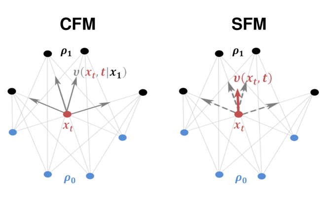
Figure 1: The key novelty of our approach is that in classical CFM, highly divergent directions can appear in a small spatial area at similar times (left part). In our approach (right part) we average over these vectors, training the model on a smoothed unnoised vector field.

1.2 Why new method?

Model training using loss (2) have the following disadvantage: during training, due to the randomness of $x_{0}$ and $x_{1}$, significantly different values can be presented for model as output value at close model argument values $(x_{t},t)$. Indeed, a fixed point $x_{t}=\phi_{t,x_{1}}\!(x_{0})$ can be obtained by an infinite set of $x_{0}$ and $x_{1}$ pairs, some of which are directly opposite, and at least for small times $t$ the probability of these different directions may not be significantly different. At the same time, data $\phi_{t,x_{1}}^{\prime}(x_{0})$ on which the model learns significantly different for such different positions of pairs $x_{0}$ and $x_{1}$. Thus, the model is forced to do two functions during training: generalize and take the mathematical expectation (clean the data from noise).

In our approach, see Fig. 1, we feed the model input with cleaned data with small variance. Thus, the model only needs to generalize the data, which happens much faster (in fewer training steps).

Moreover, in the process of constructing the modified loss, we have developed the exact formula for the vector field, see Eq. (12), (19). The existence of an explicit formula for the vector field is of great importance not only from a theoretical but also from a practical point of view.

2 Main idea

2.1 Modified objective

Lets expand the last two mathematical expectations in the loss (2) and substitute variables using map $\phi_{t,x_{1}}$, passing from the point $x_{0}$ to its position $x_{t}=\phi_{t,x_{1}}\!(x_{0})$ at time $t$:

$$\mathbb{E}_{x_{1},x_{0}}\norm{v_{\theta}(\phi_{t,x_{1}}\!(x_{0}),\,t)-\phi_{t,x_{1}}^{\prime}(x_{0})}^{2}=\\ \iint\norm{v_{\theta}(\phi_{t,x_{1}}\!(x_{0}),\,t)-\phi_{t,x_{1}}^{\prime}(x_{0})}^{2}\rho_{0}(x_{0})\rho_{1}(x_{1})\differential{x_{0}}\differential x_{1}=\\ \iint\norm{v_{\theta}(x_{t},\,t)-\phi_{t,x_{1}}^{\prime}\bigl{(}\phi_{t,x_{1}}^{-1}(x_{t})\bigr{)}}^{2}\times\\ \underbrace{\det[\evaluated{\partialderivative{\phi_{t,x_{1}}^{-1}(x)}{x}}_{x=x_{t}}]\rho_{0}\bigl{(}\phi_{t,x_{1}}^{-1}(x_{t})\bigr{)}}_{\rho_{x_{1}}(x_{t},t)}\rho_{1}(x_{1})\differential{x_{t}}\differential x_{1}=\\ \iint\norm{v_{\theta}(x_{t},\,t)-\phi_{t,x_{1}}^{\prime}\bigl{(}\phi_{t,x_{1}}^{-1}(x_{t})\bigr{)}}^{2}\times\\ \rho_{x_{1}}(x_{t},t)\rho_{1}(x_{1})\differential{x_{t}}\differential x_{1}=\\ \mathbb{E}_{x_{1},x_{t}\sim\rho_{x_{1}}(\cdot,t)}\norm{v_{\theta}(x_{t},\,t)-\phi_{t,x_{1}}^{\prime}\bigl{(}\phi_{t,x_{1}}^{-1}(x_{t})\bigr{)}}^{2}.$$ (3)

We assume, that the map $\phi_{t,x_{1}}$ is invertible at each $0<t<1$, i. e. that $\phi_{t,x_{1}}^{-1}(x_{t})$ exits on this time interval and for all $x_{t}=\{\phi_{t}(x_{0})\mid\forall x_{0}:\rho(x_{0})>0\}$. Eq. (3) can be seen as a transition from expectation on the variable $x_{0}\sim\rho_{0}$ to expectation on the variable $x_{t}\sim\rho_{x_{1}}(\cdot,t)$, where

$$\rho_{x_{1}}(x,t)=[\phi_{t,x_{1}}]_{*}\rho_{0}(x):=\rho_{0}\bigl{(}\phi_{t,x_{1}}^{-1}(x)\bigr{)}\det[\partialderivative{\phi_{t,x_{1}}^{-1}(x)}{x}].$$

See paper (Chen et al., 2018) for details about the push-forward operator “*”. Our representation (3) is very similar to expression (9) of the cited paper (Lipman et al., 2023), only we write it in terms of the conditional flow rather than the conditional vector field.

To obtain the modified loss, we return to end of the standard CFM loss representation in (3). It is written as the expectation over two random variables $x_{1}$ and $x_{t}$ having a common distribution density

$$\{x_{1},x_{t}\}\sim\rho_{j}(x_{1},x_{t},t)=\rho_{x_{1}}(x_{t},t)\rho_{1}(x_{1}),$$ (4)

which, generally speaking, is not factorizable. Let us rewrite this expectations in terms of two independent random variables, each of which have its marginal distribution. The marginal distribution $\rho_{m}$ of $x_{t}$ can be obtained via integration:

$$\rho_{m}(x_{t},t)=\int\rho_{j}(x_{1},x_{t},t)\differential{x_{1}}=\\ \int\rho_{x_{1}}(x_{t},t)\rho_{1}(x_{1})\differential{x_{1}},$$ (5)

while the marginal distribution of $x_{1}$ is just (unknown) function $\rho_{1}$. Let for convenience $w(t,x_{1},x)=\phi_{t,x_{1}}^{\prime}\bigl{(}\phi_{t,x_{1}}^{-1}(x)\bigr{)}$. We have

$$L_{\text{CFM}}(\theta)=\\ \mathbb{E}_{t,x_{1},x_{t}\sim\rho_{x_{1}}(\cdot,t)}\norm{v_{\theta}(x_{t},\,t)-w(t,x_{1},x_{t})}^{2}=\\ \int_{0}^{1}\iint\norm{v_{\theta}(x_{t},\,t)-w(t,x_{1},x_{t})}^{2}\times\\ \rho_{x_{1}}(x,t)\rho_{1}(x_{1})\differential{x_{t}}\differential x_{1}\differential t=\\ \int_{0}^{1}\iint\norm{v_{\theta}(x_{t},\,t)-w(t,x_{1},x_{t})}^{2}\times\\ \frac{\rho_{x_{1}}(x_{t},t)}{\rho_{m}(x_{t},t)}\rho_{m}(x_{t},t)\rho_{1}(x_{1})\differential{x_{t}}\differential x_{1}\differential t=\\ \mathbb{E}_{t,x_{1},x\sim\rho_{m}(\cdot,t)}\norm{v_{\theta}(x,\,t)-w(t,x_{1},x)}^{2}\times\\ \rho_{c}(x|x_{1},t)/\rho_{1}(x_{1}),$$ (6)

where we introduce a conditional distribution

$$\rho_{c}(x|x_{1},t):=\frac{\rho_{x_{1}}(x,t)\rho_{1}(x_{1})}{\rho_{m}(x,t)}:=\frac{\rho_{x_{1}}(x,t)\rho_{1}(x_{1})}{\int\rho_{x_{1}}(x,t)\rho_{1}(x_{1})\differential{x_{1}}}.$$ (7)

The key feature of the representation (6) is that the integration variables $x_{1}$ and $x$ are independent. Thus, we can evaluate them using Monte Carlo-like schemes in different ways. In particular, we can take a different number of samples for each of these variables.

However, we go further and make a modification to this loss to reduce the variance of Monte Carlo methods.

2.2 New loss and exact expression for vector field

Note that so far the expression for $L_{\text{CFM}}$ have not changed, it has just been rewritten in different forms. Now we change this expression so that its numerical value, generally speaking, may be different, but the derivative of the model parameters will be the same. We introduce the following loss

$$L_{\text{SFM}}(\theta)=\mathbb{E}_{t}\mathbb{E}_{x\sim\rho_{m}}\Bigl{\|}v_{\theta}(x,\,t)-{}\\ \mathbb{E}_{x_{1}\sim\rho_{1}}w(t,x_{1},x)\rho_{c}(x|x_{1},t)/\rho_{1}(x_{1})\Bigl{\|}^{2}=\\ \int_{0}^{1}\int\Bigl{\|}v_{\theta}(x,\,t)-\int w(t,x_{1},x)\times\\ \rho_{c}(x|x_{1},t)\differential{x_{1}}\Bigr{\|}^{2}\rho_{m}(x,t)\differential{x}\differential t.$$ (8)

Theorem 2.1.

Losses $L_{\text{CFM}}$ in Eq. (2) and $L_{\text{SFM}}$ in Eq. (8) have the same derivative with respect to model parameters:

$$\derivative{L_{\text{CFM}}(\theta)}{\theta}=\derivative{L_{\text{SFM}}(\theta)}{\theta}.$$ (9)

Proof is in the Appendix A.1.

In the presented loss $L_{\text{SFM}}$, the integration (outside the norm operator) proceeds on those variables on which the model depends, while inside this operator there are no other free variables. Thus, using this kind of loss, it is possible to find an exact analytical expression for the vector field for which the minimum of this loss is zero (unlike the loss $L_{\text{CFM}}$). Namely, we have

$$v(x,t)=\int w(t,x_{1},x)\rho_{c}(x|x_{1},t)\differential{x_{1}}.$$ (10)

We can obtain the exact form of this vector field given the particular map $\phi_{t,x_{1}}$. For example, the following statement holds:

Corollary 2.2.

Consider the linear conditioned flow

$$\phi_{t,x_{1}}\!(x_{0})=(1-t)x_{0}+tx_{1}$$ (11)

which is invertible as $0\leq t<1$. Then $w(t,x_{1},x)=\frac{x_{1}-x}{1-t}$, $\rho_{x_{1}}(x,t)=\rho_{0}\left(\frac{x-x_{1}t}{1-t}\right)\frac{1}{(1-t)^{d}}$ and the loss $L_{\text{SFM}}$ in Eq. (8) reaches zero value when the model of the vector field have the following analytical form

$$v(x,t)=\dfrac{\int(x_{1}-x)\rho_{0}\left(\frac{x-x_{1}t}{1-t}\right)\rho_{1}(x_{1})\differential{x_{1}}}{(1-t)\int\rho_{0}\left(\frac{x-x_{1}t}{1-t}\right)\rho_{1}(x_{1})\differential{x_{1}}}{}.$$ (12)

This is the exact value of the vector field whose flow translates the given distribution $\rho_{0}$ to $\rho_{1}$.

Complete proofs are in the Appendix A.3.1.

Remark 2.3.

In the case of the initial time $t=0$, Eq. (12) is noticeably simpler

$$v(x,0)=\mathbb{E}_{x_{1}}x_{1}-x=\int x_{1}\rho_{1}(x_{1})\differential{x_{1}}-x.$$ (13)

This expression for the initial velocity means that each point first tends to the center of mass of the unknown distribution $\rho_{1}$ regardless of its initial position.

Replacing the variables in (12) $y\leftarrow\frac{x-x_{1}t}{1-t}$ and taking the limit $t\to 0$ (given that $\rho_{0}$ is non-negative and integrable at infinity, and assuming that $\rho_{1}$ is bounded, see Appendix for strict derivation) we obtain a similar formula for the final time $t=1$:

$$v(x,1)=x-\int x_{0}\rho_{0}(x_{0})\differential{x_{0}}.$$ (14)

Remark 2.4.

Generalizing the previous remark, consider independent $x_{0}$ and $x_{1}$, and arbitrary mapping $\phi$. Then, $w(t=0,x_{1},x)=\phi_{0,x_{1}}^{\prime}(x)$, $\det[\partialderivative{\phi^{-1}_{0,x_{1}}\!(x)}{x}]=1$ and vectror field $v$ at the time $t=0$ equal to:

$$v(x,0)=\int\phi_{0,x_{1}}^{\prime}(x)\rho(x_{1})\differential x_{1}.$$

For any map this expression do not depend on the density $\rho_{0}$ thus, in general, there is no universal map that delivers some property which depends on both distributions. In particular, there do not exist an universal map that would perform optimal transport (OT) between all the given densities $\rho_{0}$ and $\rho_{1}$.

2.3 Training scheme based on the modified loss

Let us consider the difference between our new scheme based on loss $L_{\text{SFM}}$ and the classical CFM learning scheme. As a basis for the implementation of the learning scheme, we take the open-source code from the works (Tong et al., 2023a, b).

Consider a general framework of numerical schemes in classical CFM. We first sample $m$ random time variables $t\sim\mathcal{U}[0,1]$. Then we sample several values of $x$. To do this, we sample a certain number $n$ samples $\{x_{0}^{i}\}_{i=1}^{n}$ from the “noisy” distribution $\rho_{0}$, and the same number $n$ of samples $\{x_{1}^{i}\}_{i=1}^{n}$ from the unknown distribution $\rho_{1}$. Then we pair them (according to some scheme), and get $n$ samples as $x^{j,i}=\phi_{t^{j},x_{1}^{i}}\!(x_{0}^{i})$ (e. g. a linear combination in the simple case of linear map: $x^{j,i}=(1-t^{j})x_{0}^{i}+t^{j}x_{1}^{i}$), $\forall i=1,2,\dots,n$; $\forall j=1,2,\dots,m$. Note, than one of the variable $n$ or $m$ (or both) can be equal to $1$.

At the step 2, the following discrete loss is build using obtained samples

$$L_{\text{CFM}}^{d}(\theta)=\sum_{j=1}^{m}\sum_{i=1}^{n}\Bigl{\|}v_{\theta}(x^{j,i},\,t^{j})-\phi_{t^{j},x_{1}^{i}}^{\prime}(x_{0}^{i})\Bigr{\|}^{2}.$$ (15)

Finally, we do a standard gradient descent step to update model parameters $\theta$ using this loss.

The first and last step in our algorithm is the same as in the standard algorithm, but the second step is significantly different. Namely, we additionally generate a sufficiently large number $N\gg n\cdot m$ of samples $\overline{x}_{1}$ from the unknown distribution $\rho_{1}$, sampling $(N-n)$ new samples and adding to it the samples $\{x_{1}^{i}\}_{1}^{n}$ that are already obtained on the previous step.

The we form the following discrete loss which replaces the integral on $x_{1}$ in $L_{\text{SFM}}$ by its evaluation by importance sampling

$$L_{\text{SFM}}^{d}(\theta)=\sum_{j=1}^{m}\sum_{i=1}^{n}\Bigl{\|}v_{\theta}(x^{j,i},\,t^{j})-\\ \frac{\sum_{k=1}^{N}w(t^{j},\overline{x}_{1}^{k},x^{j,i})\rho_{\overline{x}_{1}^{k}}(x^{j,i},\,t^{j})}{\sum_{k=1}^{N}\rho_{\overline{x}_{1}^{k}}(x^{j,i},\,t^{j})}\Bigr{\|}^{2}=\\ \sum_{j=1}^{m}\sum_{i=1}^{n}\Bigl{\|}v_{\theta}(x^{j,i},\,t^{j})-v^{d}(x^{j,i},\,t^{j})\Bigr{\|}^{2},$$ (16)

where, considering that the Jacobian $\det[\partialderivative{\phi_{t,x_{1}}^{-1}(x)}{x}]$ do not depend on $x_{1}$, we can write

$$v^{d}(x,\,t)=\frac{\sum_{k=1}^{N}w(t,\overline{x}_{1}^{k},x)\rho_{0}\bigl{(}\phi^{-1}_{t,\overline{x}_{1}^{k}}\!(x)\bigr{)}}{\sum_{k=1}^{N}\rho_{0}\bigl{(}\phi^{-1}_{t,\overline{x}_{1}^{k}}\!(x)\bigr{)}}.$$

Theorem 2.5.

Under several conditions, the error variance of the integral gradient (9) using the Monte Carlo method (16) is lower than using formula (15) with the same number $n\cdot m$ of samples for $\{x\}$.

Sketch of the proof is in the Appendix A.2.

Particular case of linear map and Gaussian noise

Let $\phi_{t,x_{1}}$ be the linear flow (11). Additionally, consider the case of standard normal distribution for the initial density $\rho_{0}$: $\rho_{0}(x)\sim\mathcal{N}(x\mid 0,I)$. Then

$$v^{d}(x,\,t) =\frac{\sum_{k=1}^{N}\frac{\overline{x}_{1}^{k}-x}{1-t}\exp(Y^{k})}{\sum_{k=1}^{N}\exp(Y^{k})},$$ (17)

$$\mbox{\quad where\quad}Y^{k} =-\frac{1}{2}\frac{\norm{x-t\cdot\overline{x}_{1}^{k}}^{2}_{\mathbb{R}^{d}}}{1-t}.$$

For the linear map case with Gaussian noise, the steps of our scheme are summarized in Algorithm 1.

Algorithm 1 Vector field model training algorithm

0:  Sampler from distribution $\rho_{1}$ (or a set of samples); parameters $n$ and $m$ (number of spatial and time points, correspondingly); parameter $N$ (number of averaging point); model $v_{\theta}(x,t)$; algorithm with parameters for SGD

0:  quasi-optimal parameters $\theta$ for the trained model

1:  Initialize $\theta$ (maybe random)

2:  while exit condition is not met do

3:     Sample $m$ points $\{t^{j}\}$ from $\mathcal{U}[0,1]$

4:     Sample $n$ points pairs $\{x_{0}^{i},x_{1}^{i}\}_{i=1}^{n}$ from joint distribution $\pi$ ($\pi(x_{0},x_{1})=\rho_{0}(x_{0})\rho_{1}(x_{1})$ if variables are independent)

5:     Sample $N-n$ points $\{\hat{x}_{1}^{l}\}$ from $\rho_{1}$ and form $\{\overline{x}_{1}^{k}\}=\{x_{1}^{i}\}\cup\{\hat{x}_{1}^{l}\}$ // We can take all available samples as $\{\overline{x}_{1}^{k}\}$ if we don’t have access to a sampler, but only ready-made samples.

6:     For all $i$ and $j$ calculate the sum at the right side of (16) (using (17) if $\rho_{0}$ is standard Gaussian or (28) in general)

7:     Calculate the sum on $i$ and $j$ in discrete loss (16), and take backward derivative, obtaining approximate grad $G\approx\gradient_{\theta}L_{\text{SFM}}$ of loss $L_{\text{SFM}}$ on model parameters $\theta$.

8:     Update model parameters $\theta\leftarrow SGD(\theta,G)$

9:  end while

Extension of other maps and initial densities $\rho_{0}$

When using other maps, formula (12) is modified accordingly. For example, if we use the regularized map $\phi_{t,x_{1}}\!(x_{0})=(1-t)x_{0}+tx_{1}+\sigma_{s}tx_{0}$, we get the formula (30) given in Appendix. Note, that in this case the final density $\rho(x,\,1)$, obtained from the continuity equation is not equal to $\rho_{1}$, but is its smoothed modification.

When using a different initial density $\rho_{0}$ (not the normal distribution), an obvious modification will be made to formula (17).

Moreover, in addition to the independent densities $x_{0}\sim\rho_{0}$ and $x_{1}\sim\rho_{1}$, we can use the joint density $\{x_{0},\,x_{1}\}\sim\pi(x_{0},\,x_{1})$. In the papers (Tong et al., 2023a, b), optimal transport (OT) and Schrödinger’s bridge are taken as $\pi$. In this case the expression for the vector field changes insignificantly: the conditional probability $\rho_{c}$ from Eq. (7) is subject to change:

$$\rho_{c}(x|x_{1},t)=\frac{\pi\left(\phi_{t,x_{1}}^{-1}(x),x_{1}\right)\det[\partialderivative{\phi_{t,x_{1}}^{-1}(x)}{x}]}{\int\pi\left(\phi_{t,x_{1}}^{-1}(x),x_{1}\right)\det[\partialderivative{\phi_{t,x_{1}}^{-1}(x)}{x}]\differential{x_{1}}}.$$ (18)

Then, Eq. (10) remains the same in general case. In the case of linear $\phi$, the extension of Eq. (12) reads

$$v(x,t)=\dfrac{\int(x_{1}-x)\,\pi\!\left(\phi_{t,x_{1}}^{-1}(x),x_{1}\right)\det[\partialderivative{\phi_{t,x_{1}}^{-1}(x)}{x}]\differential{x_{1}}}{(1-t)\int\pi\!\left(\phi_{t,x_{1}}^{-1}(x),x_{1}\right)\det[\partialderivative{\phi_{t,x_{1}}^{-1}(x)}{x}]\differential{x_{1}}}{}.$$ (19)

In all of the above cases, the essence of Algorithm 1 does not change (except that in the case of dependent $x_{0}$ and $x_{1}$ we should be able either to calculate the value of $\pi\!\left(\phi_{t,x_{1}}^{-1}(x),x_{1}\right)/\rho_{1}(x_{1})$ or to estimate it).

Complexity

We assume that the main running time of the algorithm is spent on training the model, especially if it is quite complex. Thus, the running time of one training step depends crucially on the number $n\cdot m$ of samples $\{x\}$ and and it is approximately the same for both algorithms: the addition of points $\overline{x}_{1}$ entails only an additional calculation using formula (17), which can be done quickly and, moreover, can be simple parallelized.

The main advantage of our algorithm, as shown by experiments, is significantly reducing the number of steps to achieve the same learning accuracy.

2.4 Irreducible dispersion of gradient for CFM optimization

Ensuring the stability of optimization is vital. The main aspect is the analysis of the dispersion of model update $\delta v_{\theta}$. Let $\Delta\theta$ be changes in parameters, obtained by SGD with step size $\gamma/2$ applied to the functional from Eq. (15):

$$\Delta\theta=-\gamma\sum_{j=1}^{m}\sum_{i=1}^{n}\bigl{(}v_{\theta}(x^{j,i},\,t^{j})-\phi_{x_{1}^{i},t^{j}}^{\prime}(x_{0}^{i})\bigr{)}^{T}\frac{\differential v_{\theta}(x^{j,i},\,t^{j})}{\differential\theta}$$

Then, we can write (the index $\theta$ will be omitted here for brevity)

$$\Delta v(x^{j,i},t^{j})=-\gamma\cdot\bigl{(}v(x^{j,i},t^{j})-\phi_{x_{1}^{i},t^{j}}^{\prime}(x_{0}^{i})\bigr{)}.$$ (20)

Accordingly, using the proposed scheme (16), we have:

$$\Delta v(x^{j,i},t^{j})=-\gamma\cdot\bigl{(}v(x^{j,i},t^{j})-v^{d}(x^{j,i},\,t^{j})\bigr{)}.$$ (21)

For simplification, we consider a function, $v_{\theta}(x,t)$, capable of perfectly fitting the CFM problem and providing an optimal solution for any point $x$ and time $t$.

The standard CFM’s loss does not reach zero at its minimum even for definition through integrals (2), leading to noisy update of the form (20) at each step, even with a perfectly trained model.

Our loss reaches a minimum of zero, ensuring that the model remains unchanged in the next SGD steps. This results in smaller variance of the updates compared to the standard CFM. In other words, right-hand side of (21) reaches zero at ideal model, and during training, its magnitude (and variance) is smaller than those of (20).

In actual numerical approximations (losses (15) and (16)), the difference in dispersions between the real losses is smaller than in ideal conditions, especially as the value of t approaches 1. This is due to a poor approximation of the integral over $x_{1}$, as the sum over individual points poorly approximates the integral around the point $t=1$, leading to the breakdown of the importance sampling condition.

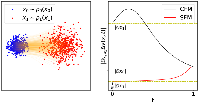
Figure 2: The comparison evaluated dispersion norm over time parameter $t$ for CFM and SFM in matching standard Gaussian $\rho_{0}\sim\mathcal{N}(0,I)$ to general Gaussian $\rho_{1}\sim\mathcal{N}(\mu,\sigma^{2}I)$ distributions. The y-axis represents the sum of dispersion vector components, denoted as $|\mathbb{D}_{x,x_{1}}\Delta v(x,t)|$. The left panel illustrates samples drawn from the $\rho_{0}$ and $\rho_{1}$ distributions, as well as the corresponding flows. The right panel depicts the dispersion trend over time for both CFM (black line) and SFM (red line) objectives. The dotted lines correspond to the dispersion levels (in top-down order $|\mathbb{D}x_{1}|$, $|\mathbb{D}x_{0}|$, $|\mathbb{D}x_{1}|/N$.

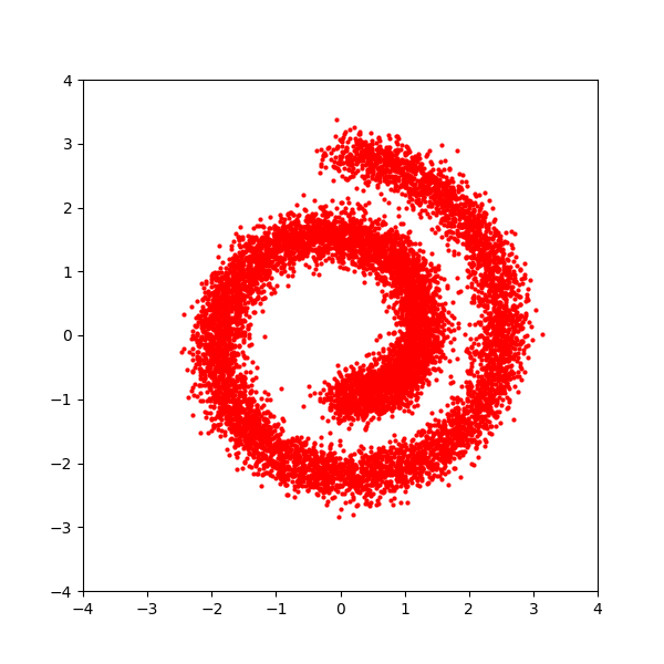
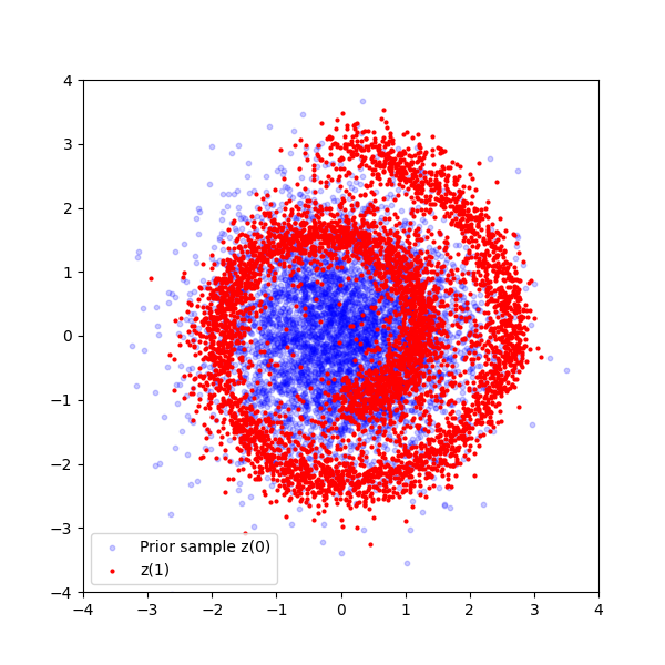
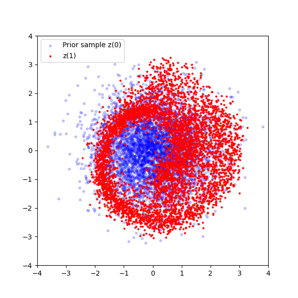
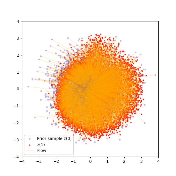
(a) swissroll

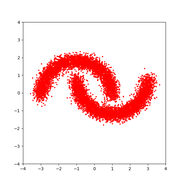
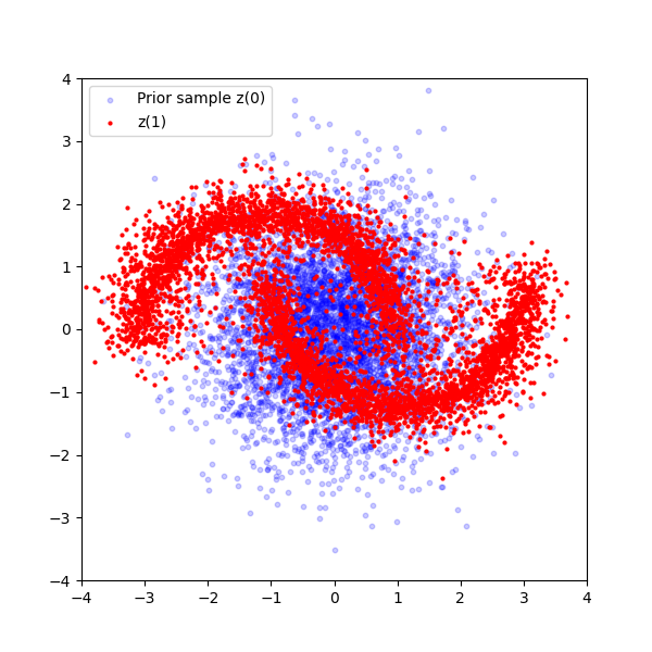
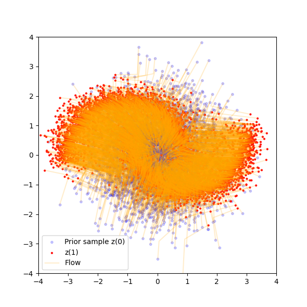
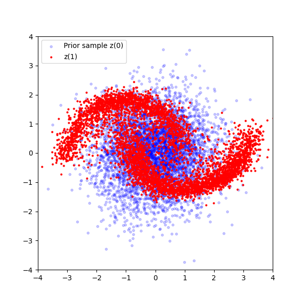
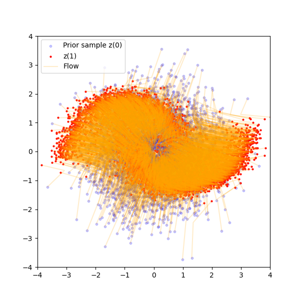
(b) moons

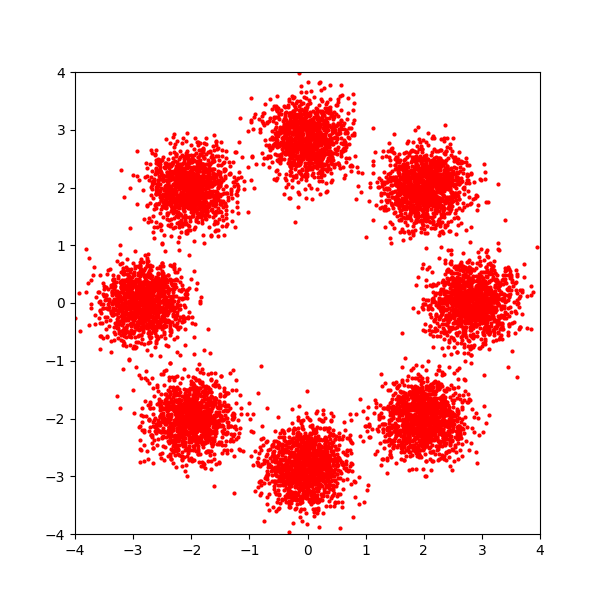
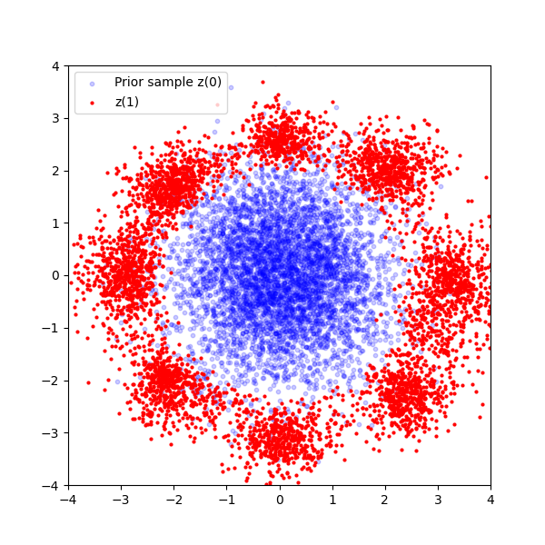
(c) 8gaussians

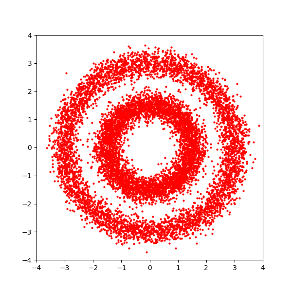
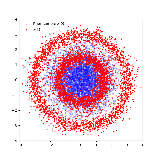
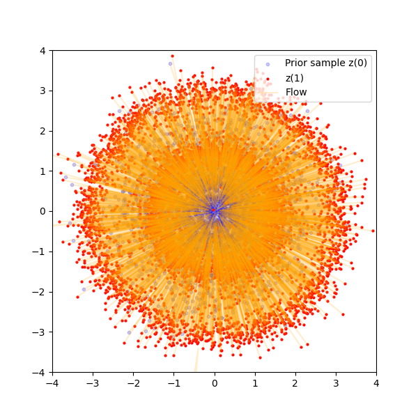
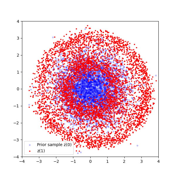
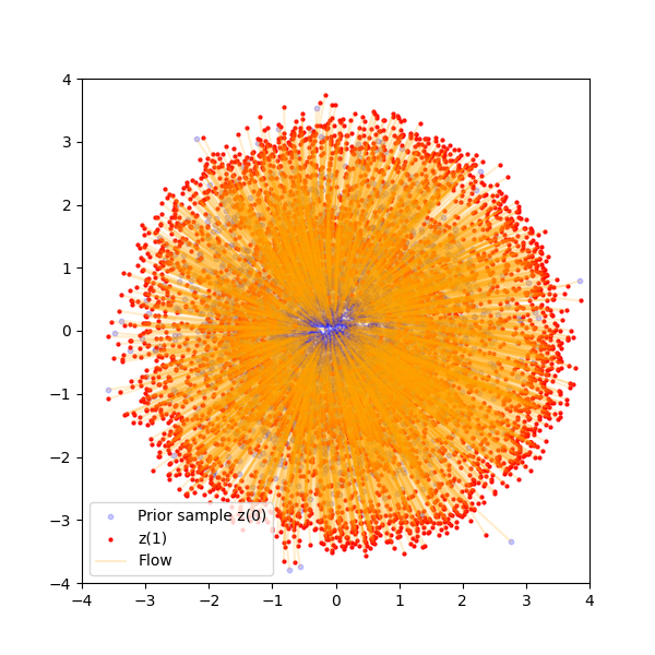
(d) circles

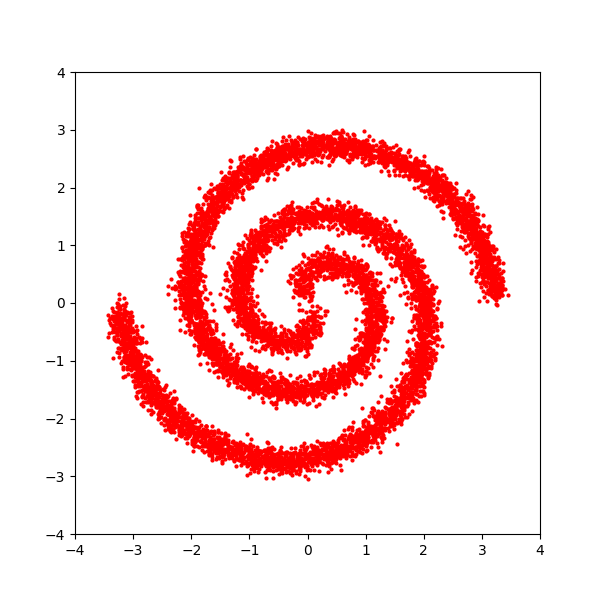
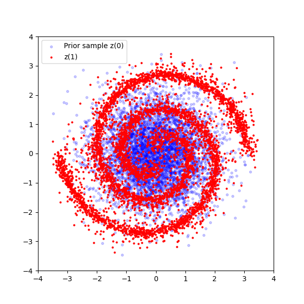
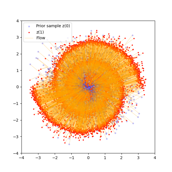
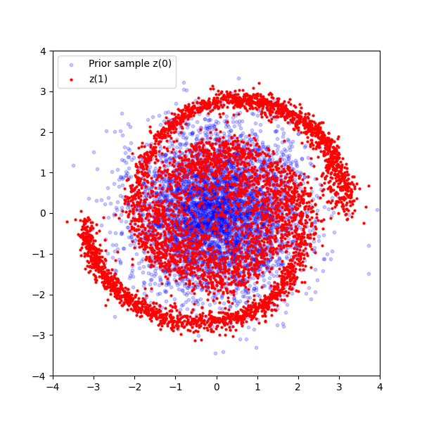
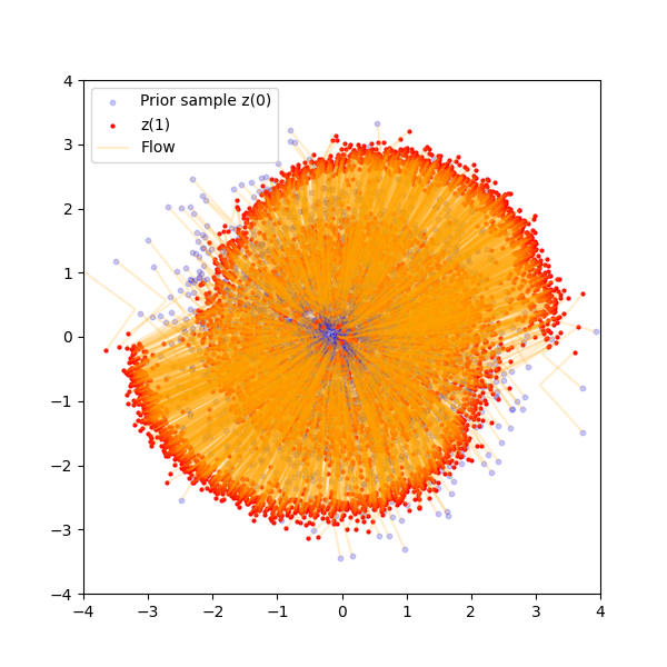
(e) 2spirals

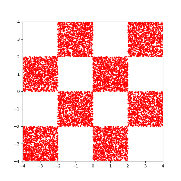
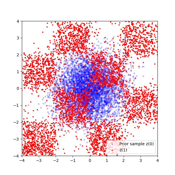
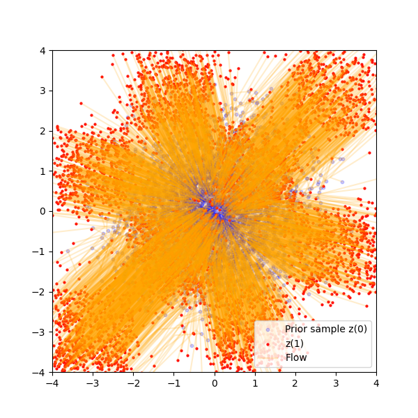
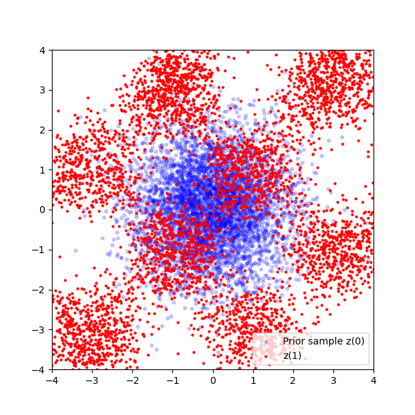
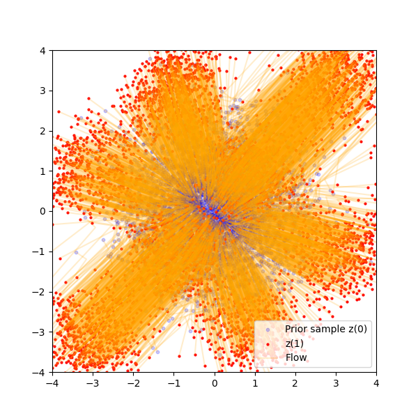
(f) checkerboard

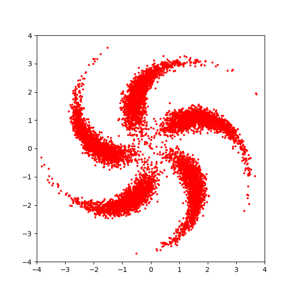
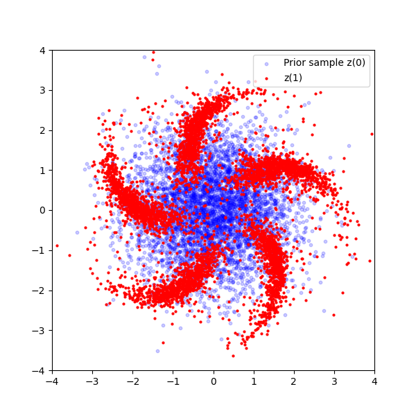
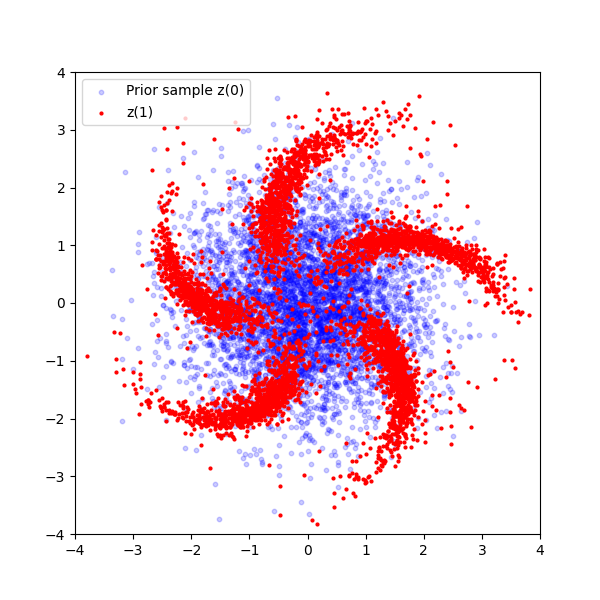
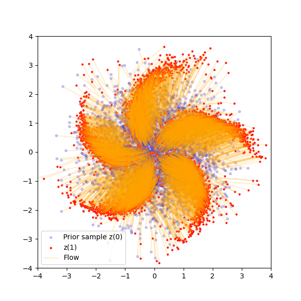
(g) pinwheel

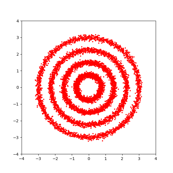
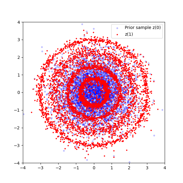
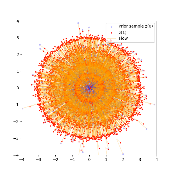
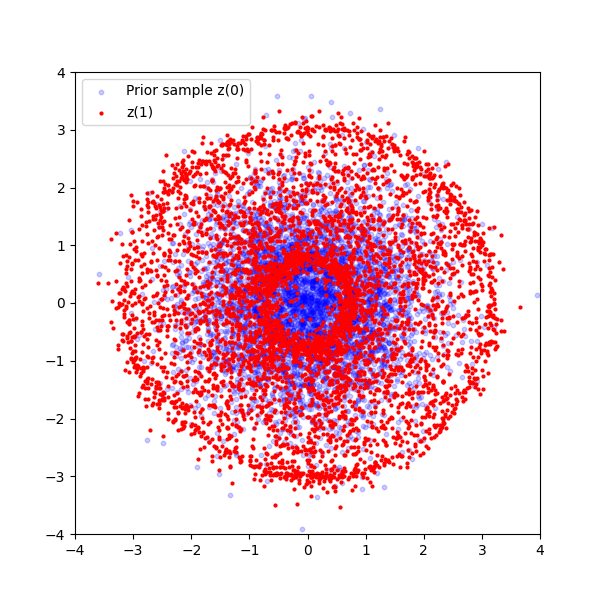
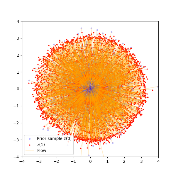
(h) rings

Figure 3: Visual comparison of methods on toy 2D data. First row are original samples, second row sampled by SFM, third row sampled by SFM with trajectories, fourth row sampled by CFM, fifth row sampled by CFM with trajectories.

	MSE training loss		Energy Distance
Data	SFM	CFM	SFM	CFM
swissroll	1.13e-02	2.12e+00	2.58e-03	1.07e-02
moons	9.96e-03	2.01e+00	2.74e-03	1.41e-02
8gaussians	2.40e-02	2.77e+00	4.90e-03	2.45e-02
circles	9.28e-03	2.79e+00	6.69e-04	1.32e-02
2spirals	8.92e-03	2.34e+00	1.27e-03	8.35e-03
checkerboard	1.04e-02	3.12e+00	1.01e-02	1.63e-02
pinwheel	4.53e-03	2.12e+00	1.01e-03	9.22e-03
rings	8.60e-03	1.93e+00	3.55e-04	2.37e-03

Table 1: SFM and CFM metrics comparison table on toy 2D data.

	MSE training loss		NLL
Data	SFM	CFM	SFM	CFM
power	9.93e-03	1.05e+00	7.45e+00 $\pm$ 1.82e-02	8.58e+00 $\pm$ 1.67e-01
gas	1.56e-02	9.55e-01	9.05e+00 $\pm$ 3.00e-02	1.15e+01 $\pm$ 1.45e-01
hepmass	1.18e-01	1.44e+00	2.43e+01 $\pm$ 1.31e-01	3.00e+01 $\pm$ 3.13e-01
bsds300	6.67e-03	1.14e-01	6.30e+01 $\pm$ 9.42e-02	8.91e+01 $\pm$ 9.99e-01
miniboone	2.87e-01	1.25e+00	4.92e+01 $\pm$ 3.04e-01	6.06e+01 $\pm$ 1.07e+00

Table 2: SFM and CFM metrics comparison table on Tabular data, taken mean and std through 10 experiments.

Dispersion analysis

For a linear conditional flow at a specific point $x^{j,i}\sim\rho_{x_{1}^{i}}(\cdot,t^{j})$ at time $t^{j}\sim U(0,1)$, the update $\Delta v(x^{j,i},t^{j})$ can be represented as follows:

$$\Delta v(x^{j,i},t^{j})=\gamma\left(x_{1}^{i}-\hat{x}_{0}^{i}-v(x^{j,i},t^{j})\right),$$ (22)

where $\hat{x}_{0}^{i}=\frac{x^{j,i}-t^{j}x_{1}^{i}}{1-t^{j}}$. We define the dispersion $\mathbb{D}_{x,x_{1}}f(x,x_{1})$ for $x\sim\rho_{x_{1}}(\cdot,t)$ and $x_{1}\sim\rho_{1}$ as:

$$\mathbb{D}_{x,x_{1}}f(x,x_{1})=\mathbb{E}_{x,x_{1}}f^{2}(x,x_{1})-(\mathbb{E}_{x,x_{1}}f(x,x_{1}))^{2}.$$ (23)

Proposition 2.6.

At the time $t=0$, the dispersion of update in the form (22) have the following element-wise lower bound:

$$\mathbb{D}_{x^{j,i},x_{1}^{i}}\Delta v(x^{j,i},0)=\gamma^{2}\mathbb{D}_{x_{1}^{i}}x_{1}^{i}+\\ \gamma^{2}\mathbb{D}_{x^{j,i},x_{1}^{i}}(x^{j,i}+v(x^{j,i},0))\geq\gamma^{2}\mathbb{D}_{x_{1}^{i}}x_{1}^{i}.$$

Equality is reached when the model $v(x^{j,i},0)$ has exact values equal to (13).

From the analysis, two key observations can be made:

• The dispersion of the update is directly proportional to the dispersion of the target distribution.

• The dispersion is independent of the batch size used.

These insights shed light on the applicability of CFM. Given that the dispersion cannot be reduced with an increase in batch size, the only available option is to decrease the step size of the optimization method, i. e., reduce the learning rate. While this approach enhances the stability of the optimization, it also slows down the convergence. For target distributions with high dispersion, a more substantial reduction in the step size is necessary for improvement.

Comparison with SFM

Using the equation (16), we can express the update $\Delta v(x^{j,i},t^{j})$ in the case of SFM objective as:

$$\Delta v(x^{j},t^{j})=\gamma^{2}\Bigl{(}\sum\limits_{k=1}^{N}x_{1}^{k}\tilde{\rho}\left(x^{j,i}|x_{1}^{k},t^{j}\right)-\\ x^{j,i}-v(x^{j,i},t^{j})\Bigr{)},$$ (24)

where $x^{j,i}\sim\rho_{x_{1}^{i}}(\cdot,t^{j})$, $x_{1}^{k}\sim\rho_{1}$ and $\tilde{\rho}\left(x^{j,i}|x_{1}^{k},t^{j}\right)=\rho_{0}\left(\frac{x^{j,i}-t^{j}x_{1}^{k}}{1-t^{j}}\right)/\sum\limits_{k=1}^{N}\rho_{0}\left(\frac{x^{j,i}-t^{j}x_{1}^{k}}{1-t^{j}}\right)$. Similar to the derivations in the previous part, we can found simplified form for the dispersion of update at $t=0$. For $t=0$ coefficients

$$\tilde{\rho}\left(x^{j,i}|x_{1}^{k},t^{j}\right)=\frac{1}{N},\quad\mathbb{D}_{x_{1}^{k}}\sum\limits_{k=1}^{N}x_{1}^{k}=N\mathbb{D}_{x_{1}^{k}}x_{1}^{k},$$

$x^{j,i}=x_{0}^{j,i}$ and $v(x^{j,i},t^{j})$ are independent of $x_{1}^{k}$.

Proposition 2.7.

At the time $t=0$, the dispersion of update from (24) have the following element-wise lower bound:

$$\mathbb{D}_{x^{j,i},x_{1}^{k}}\Delta v(x^{j,i},0)=\frac{\gamma^{2}}{N}\mathbb{D}_{x_{1}^{k}}x_{1}^{k}+\\ \gamma^{2}\mathbb{D}_{x^{j,i},x_{1}^{k}}(x^{j,i}+v(x^{j,i},0))\geq\frac{\gamma^{2}}{N}\mathbb{D}_{x_{1}^{k}}x_{1}^{k}.$$

Equality is reached when the model $v(x^{j,i},0)$ has exact values equal to (13).

The key distinction from CFM is that the dispersion of the update is $N$ times smaller than the dispersion of the target distribution. This provides the ability to control the stability of optimization without impeding convergence by adjusting the number of samples $N$. A higher value of $N$ leads to a more stable convergence to the optimal solution. In Figure 2, we visually compare the dispersions of CFM and SFM. The illustration aligns a standard normal distribution $\mathcal{N}(0,I)$ with a shifted and scaled variant $\mathcal{N}(\mu,I\sigma^{2})$. At $t=0$, the SFM update dispersion is $N$ times smaller than that of CFM, and overall, SFM yields lower dispersion throughout the range $t\in[0,1]$. Detailed analytical calculations of the optimal velocity $v(x,t)$ and dispersions are provided in the Appendix.

3 Details of Numerical Experiments

3.1 Toy 2D data

We conducted unconditional density estimation among eight distributions. Additional details of the experiments see in the Appendix B.

We commence the exposition of our findings by showcasing a series of classical 2-dimensional examples, as depicted in Fig. 3 and Table 1. Our observations indicate that SFM adeptly handles complex distribution shapes is particularly noteworthy, especially considering its ability to do so within a small number of epochs. Additionally, the visual comparison underscores the evident superiority of SFM over the CFM approach. This highlights the robustness and effectiveness of SFM in addressing the challenges posed by complex distributions.

3.2 Tabular data

We conducted unconditional density estimation on five tabular datasets, namely power, gas, hepmass, minibone, and BSDS300. Additional details of the experiments see in the Appendix B.

The empirical findings obtained from the numerical experiments from Table 2 indicate a statistically significant improvement in the performance of our proposed method. Notably, SFM demonstrates a notable acceleration in convergence rate, particularly in scenarios involving high-dimensional datasets.

4 Related work

All the aforementioned papers explore various techniques for simulation-free training in the field of Continuous Normalizing Flows (CNFs). One such approach, proposed by (Lipman et al., 2023) leverages non-diffusion probability paths to train CNFs, introducing Conditional Flow Matching method. On a similar note, (Liu et al., 2022) present Rectified Flow, a method that establishes connections between samples using straight paths and learns an ODE model for training. By employing a ”reflow” operation, the ODE trajectories are iteratively straightened to achieve one-step generation. In the pursuit of simulation-free training, (Tong et al., 2023b) method entails the use of a simulation-free score and flow matching objective, enabling the inference of stochastic dynamics from unpaired source and target samples drawn from arbitrary distributions. (Tong et al., 2023a) propose an approach where couplings between data and noise samples are established while ensuring compliance with correct marginal constraints. In (Pooladian et al., 2023) introduced the establishment of couplings between data and noise samples by concurrent compliance with appropriate marginal constraints. For training CNFs on manifolds, (Chen & Lipman, 2023) present a simulation-free approach specifically tailored for simple geometries. Divergence computation is not necessary in this method, as the target vector field is computed in closed form. An alternative methodology, proposed by (Jolicoeur-Martineau et al., 2023), involves the utilization of Gradient-Boosted Trees (GBTs) to estimate the vector field or score-function for the generation and imputation of mixed-type tabular data. This approach incorporates discrete noise levels and random Gaussian noise to calculate noisy samples via the forward diffusion/flow step.

5 Conclusion and future work

The presented method introduces a new loss function (in terms of expectations) that improves upon the existing Conditional Flow Matching approach. The gradient of the SFM loss on the parameter of the model is the same as gradient of the usual CFM loss. Thus, the argument minimums (vector field) of the considered two losses are the same. But new loss as a function of the model parameters, reaches zero at its minimum. Thanks to this, we can:

• write an explicit expression for the vector field on which the loss minimum is achieved;

• get a smaller variance when training on the discrete version of the loss, therefore, we can learn the model faster and more accurately.

Numerical experiments conducted on toy 2D data show reliable outcomes under uniform conditions and parameters. Comparison of the absolute values of loss for the proposed method and for CFM for the same distributions show that the absolute values of loss for these models differ strikingly, by a factor of $10^{2}$–$10^{3}$.

Additionally, algebraic analysis of variance for some cases (in particular, for the case $t=0$ or for the case of two Gaussians as initial and final distributions) show an improvement in variance when using the new loss. However, it is rather difficult to analyze in the general case, for all times t and general distributions $\rho_{0}$ and $\rho_{1}$.

As future works we point out the theoretical use of the explicit formula for the vector field in order to study the properties of Flow Matching and its modifications, as well as the invention of new numerical schemes using this formula.

Appendix A Proof of the theorems

A.1 Proof of the Theorem 2.1

Proof.

We need to proof, that $\derivative{L_{\text{CFM}}(\theta)}{\theta}=\derivative{L_{\text{SFM}}(\theta)}{\theta}$.

To establish the equivalence of $L_{\text{CFM}}$ and $L_{\text{SFM}}$ up to a constant term, we begin by expressing $L_{\text{CFM}}$ in the format specified by equation (6):

$$L_{\text{CFM}}=\mathbb{E}_{t,x_{1},x\sim\rho_{m}(\cdot,t)}\norm{v_{\theta}(x,\,t)-w(t,x_{1},x)}^{2}\times\\ \rho_{c}(x|x_{1},t)/\rho_{1}(x_{1}).$$

Utilizing the bilinearity of the 2-norm, we can rewrite $L_{\text{CFM}}$ as:

$$L_{\text{CFM}}=\mathbb{E}_{t,x_{1},x\sim\rho_{m}(\cdot,t)}\frac{\norm{v_{\theta}(x,\,t)}^{2}\rho_{c}(x|x_{1},t)}{\rho_{1}(x_{1})}-{}\\ 2\mathbb{E}_{t,x_{1},x\sim\rho_{m}(\cdot,t)}\frac{v_{\theta}(x,\,t)^{T}\cdot w(t,x_{1},x)\rho_{c}(x|x_{1},t)}{\rho_{1}(x_{1})}+C.$$ (25)

Here, $T$ denotes transposed vector, dot denotes scalar product, $C$ represents a constant independent of $\theta$.

Noting that $\mathbb{E}_{x_{1}}\rho_{c}(x|x_{1},t)/\rho_{1}(x_{1})=1$:

$$\mathbb{E}_{x_{1}}\frac{\rho_{c}(x|x_{1},t)}{\rho_{1}(x_{1})}=\int\frac{\rho_{x_{1}}(x,t)\rho_{1}(x_{1})\differential{x_{1}}}{\int\rho_{x_{1}}(x,t)\rho_{1}(x_{1})\differential{x_{1}}}=1,$$

we can simplify the first term in the expansoin (25):

$$\mathbb{E}_{t,x_{1},x\sim\rho_{m}(\cdot,t)}\frac{\norm{v_{\theta}(x,\,t)}^{2}\rho_{c}(x|x_{1},t)}{\rho_{1}(x_{1})}=\\ E_{t,x\sim\rho_{m}(\cdot,t)}\norm{v_{\theta}(x,\,t)}^{2}\,\mathbb{E}_{x_{1}}\frac{\rho_{c}(x|x_{1},t)}{\rho_{1}(x_{1})}=\\ E_{t,x\sim\rho_{m}(\cdot,t)}\norm{v_{\theta}(x,\,t)}^{2}.$$ (26)

For our loss $L_{\text{SFM}}$ in the form (8) we also use the bilinearity of the norm:

$$L_{\text{SFM}}=\mathbb{E}_{t,x\sim\rho_{m}(\cdot,t)}\norm{v_{\theta}(x,\,t)}^{2}-{}\\ 2\mathbb{E}_{t,x\sim\rho_{m}(\cdot,t)}\mathbb{E}_{x_{1}}\frac{v_{\theta}(x,\,t)^{T}\cdot w(t,x_{1},x)\rho_{c}(x|x_{1},t)}{\rho_{1}(x_{1})}+C.$$ (27)

Comparing the last expression and the Eq. (25) with the modification (26) and also taking into account the independence of random variables $x$ and $x_{1}$, we come to the conclusion that $L_{\text{SFM}}$ is equal to $L_{\text{CFM}}$ up to some constant independent of the model parameters.

∎

A.2 Sketch of the proof of the Theorem 2.5

Proof.

We need to prove that $\mathbb{D}\derivative{L_{\text{SFM}}^{d}(\theta)}{\theta}\leq\mathbb{D}\derivative{L_{\text{CFM}}^{d}(\theta)}{\theta}$, where $L_{\text{SFM}}^{d}(\theta)$ and $L_{\text{CFM}}^{d}(\theta)$ discrete loss functions presented in (16) and (15). Firstly, let us rewrite the derivative of loss functions using the bilinearity:

$$\derivative{L_{\text{SFM}}^{d}(\theta)}{\theta}=2\sum\limits_{i,j}\left(\derivative{v_{\theta}(x^{j,i},\,t^{j})}{\theta}\right)^{T}\cdot\\ \bigl{(}v_{\theta}(x^{j,i},\,t^{j})-v^{d}(x^{j,i},t^{j})\bigr{)}.$$

Note that in this expression, values $x^{j,i}$ as well as $t^{j}$, which are included in the argument of the function $v$, are fixed (our goal to calculate the variance with fixed model arguments). Thus, we need to consider the variance of the remaining expression arising from the randomness of $\overline{x}_{1}^{k}$.

Recall (below we will omit the indices at variables $x$ and $t$),

$$v^{d}(x,\,t)=\frac{\sum_{k=1}^{N}w(t,\overline{x}_{1}^{k},x)\cdot\rho_{0}\bigl{(}\phi^{-1}_{t,\overline{x}_{1}^{k}}\!(x)\bigr{)}}{\sum_{k=1}^{N}\rho_{0}\bigl{(}\phi^{-1}_{t,\overline{x}_{1}^{k}}\!(x)\bigr{)}}.$$

Note, that if $N=1$, (i. e. we do not sample any additional points other than the ones we have already sampled) this expression is exactly the same as the derivative of the common discretized CFM loss $\derivative{L_{\text{CFM}}^{d}(\theta)}{\theta}$.

Moreover, recall that one of the points (without loss of generality, we can assume that its index is 1) $\overline{x}_{1}^{1}$ is added from the set from which point $x$ was derived: $x=\phi_{t,\overline{x}_{1}^{1}}\!(x_{0})$. (Here $x_{0}$ is the paired point to $\overline{x}_{1}^{1}$)

Thus, we can rewrite expression for $v^{d}$:

$$v^{d}(x,\,t)=\\ \frac{w(t,\overline{x}_{1}^{1},x)\rho_{0}(x_{0})+\sum_{k=2}^{N}w(t,\overline{x}_{1}^{k},x)\cdot\rho_{0}\left(\phi^{-1}_{t,\overline{x}_{1}^{k}}\!(x)\right)}{\rho_{0}(x_{0})+\sum_{k=2}^{N}\rho_{0}\left(\phi^{-1}_{t,\overline{x}_{1}^{k}}\!(x)\right)}.$$ (28)

Thus, our task was reduced to evaluating how well the additional terms (for $k$ starting from $2$) improve approximate of the original integrals that are in loss (8).

So, we need to estimate the following dispersion ratio, where in the numerator is the variance of discrete loss CFM, and in the denominator — the variance of loss SFM:

$$k_{D}=\frac{\mathbb{D}\bigl{(}v_{\theta}(x,t)-w(t,\overline{x}_{1}^{1},x)\bigr{)}}{\mathbb{D}\left(v_{\theta}(x,t)-\frac{\sum_{k=1}^{N}w(t,\overline{x}_{1}^{k},x)\cdot\rho_{0}\bigl{(}\phi^{-1}_{t,\overline{x}_{1}^{k}}\!(x)\bigr{)}}{\sum_{k=1}^{N}\rho_{0}\bigl{(}\phi^{-1}_{t,\overline{x}_{1}^{k}}\!(x)\bigr{)}}\right)}$$

The smaller coefficient $k_{D}$ is, the better the proposed loss SFM works.

Formally, we can write our problem as an importance sampling problem for the following integral:

$$I=\int f(x)p(x)\differential{x}.$$

This integral we estimate by sample mean of the following expectation over some random variable with density function $q(x)$:

$$I=\mathbb{E}_{x\sim q}\bigl{(}w(x)f(x)\bigr{)}$$

with

$$w(x)=\frac{p(x)}{q(x)}.$$

We replace the exact value of $I$ with the value

$$\overline{I}=\frac{\sum_{k=1}^{N}w(\overline{x}_{1}^{i})f(\overline{x}_{1}^{k})}{\sum_{i=k}^{N}w(\overline{x}_{1}^{k})}.$$

It follows from the strong law of large numbers that in the limit $N\to\infty$, $I\to\overline{I}$ almost surely. From the central limit theorem we can find the asymptotic variance:

$$\mathbb{D}\overline{I}=\frac{1}{N}\mathbb{E}_{x\sim q}\bigl{(}w^{2}(x)(f(x)-I)^{2}\bigr{)}.$$ (29)

In our case (loss $L_{\text{SFM}}$), we have $q(x_{1})=\rho_{1}(x_{1})$, $f(x_{1})=w(t,x_{1},x)$ and $w(x_{1})=\rho_{0}\left(\phi^{-1}_{t,x_{1}}\!(x)\right)$.

Despite the fact that the equation (29) for the variance contains $N$ in the denominator, it is rather difficult to give an estimate of its behavior in general. The point is that this formula is well suited for the case when $w$ in it is of approximately the same order. In the considered case, this is achieved at times $t$ noticeably less than $1$.

But in the case, when $t$ is closed to $1$ we have, for example, for the linear map, that

$$w(x_{1})=\rho_{0}\left(\phi^{-1}_{t,x_{1}}\!(x)\right)=\rho_{0}\left(\frac{x-x_{1}t}{1-t}\right)$$

and this function has a sharp peak near the point $x/t$ if it is considered as a function of $x_{1}$. Thus, at such values of $t$, only a small number of summands will give a sufficient contribution to the sum compared to the first term.

Finally, inequality $k_{D}<1$ is formally fulfilled, but how much $k_{D}$ is less than one depends on many factors.

∎

A.3 Expressions for the regularized map

To justify the expression (12), we use a invertable transformation and then strictly take the limit $\sigma_{s}\to 0$.

Expression Eq. (12), (17) are obtained for the simple map $\phi_{t,x_{1}}\!(x_{0})=(1-t)x_{0}+tx_{1}$ which is not invertable at $t=1$. For the map with small regaluraziting parameter $\sigma_{s}>0$ $\phi_{t,x_{1}}\!(x_{0})=(1-t)x_{0}+tx_{1}+\sigma_{s}x_{0}$, which is invertable at all time values $0\leq t\leq 1$, Eq. (12), (17) needs modifications. Namely, for this map the following exact formulas holds true

$$v(x,t)=\int w(t,x_{1},x)\rho_{c}(x|x_{1},t)\rho_{1}(x_{1})\differential{x_{1}}=\\ \dfrac{\int\bigl{(}x_{1}-x(1-\sigma_{s})\bigr{)}\rho_{0}\left(\frac{x-x_{1}t}{1+\sigma_{s}t-t}\right)\rho_{1}(x_{1})\differential{x_{1}}}{(1+\sigma_{s}t-t)\int\rho_{0}\left(\frac{x-x_{1}t}{1+\sigma_{s}t-t}\right)\rho_{1}(x_{1})\differential{x_{1}}}{}.$$ (30)

By direct substitution we make sure that for this vector field

$$v(x,\,0)=\int x_{1}\rho_{1}(x_{1})\differential{x_{1}}-x(1-\sigma_{s})$$

and

$$v(x,\,1)=\dfrac{\int(x-y)\rho_{0}(y)\rho_{1}(x-y\sigma_{s})\differential{y}}{\int\rho_{0}(y)\rho_{1}(x-y\sigma_{s})\differential{y}}{},$$ (31)

where we perform change of the variables $y\leftarrow\frac{x_{1}-x}{\sigma_{s}t}$.

A.3.1 Prof of the explicit formula (12) for the vector field

Assumption A.1.

Density $\rho_{1}$ is continuous at any point $x\in(-\infty,\,\infty)$.

Theorem A.2.

In equations (30) and (31) we can take the limit $\sigma_{s}\to 0$ under integrals to get Eq. (12) and (14).

Proof.

Assuming that the distribution $\rho_{1}$ has a finite first moment: $|\int\xi\rho_{1}(\xi)\differential{\xi}|<C_{1}$ and that the density of $\rho_{0}$ is bounded: $\rho_{0}(x)<C_{2}$, $\forall x\in(-\infty,\infty)$, we obtain that the integrand functions in the numerator and denominator in the Eq. (30) can be bounded by the following integrable functions independent of $\sigma_{s}$ and $t$:

$$\rho_{0}\left(\frac{x-x_{1}t}{1+\sigma_{s}-t}\right)\rho_{1}(x_{1})<C_{1}\rho_{1}(x_{1})$$

and

$$0 \leq x_{1}\rho_{0}\left(\frac{x-x_{1}t}{1+\sigma_{s}t-t}\right)\rho_{1}(x_{1})<x_{1}C_{1}\rho_{1}(x_{1}), x \geq 0,$$

$$0 >x_{1}\rho_{0}\left(\frac{x-x_{1}t}{1+\sigma_{s}t-t}\right)\rho_{1}(x_{1})>x_{1}C_{1}\rho_{1}(x_{1}), x <0.$$

It follows that both integrals in expression (30) converge absolutely and uniformly. So, we can swap the operations of taking the limit and integration, and we can take the limit $\sigma_{s}\to 0$ in the integrand for any time $t\in[0,\,t_{0}]$ for arbitrary $t_{0}<1$.

Now, let us consider the case $t=1$. From Assumption A.1 the boundedness of the density $\rho_{1}$ follows: $\rho_{1}(x)<C_{2}$, $\forall x\in(-\infty,\,\infty)$. Thus, integrand functions in the numerator and denominator in the Eq. (31) can be bounded by the following integrable functions independent of $\sigma_{s}$:

$$\rho_{0}(y)\rho_{1}(x-y\sigma_{s})<\rho_{0}(y)C_{2}$$

and

$$0 \leq y\rho_{0}(y)\rho_{1}(x-y\sigma_{s})<yC_{2}\rho_{0}(y), y \geq 0,$$

$$0 >y\rho_{0}(y)\rho_{1}(x-y\sigma_{s})>yC_{2}\rho_{0}(y), y <0.$$

The existence of the limit

$$\lim_{\sigma_{s}\to 0}\rho_{1}(x-y\sigma_{s})=\rho_{1}(x),$$

follows from Assumption A.1.

Finally, we conclude that formula (12), regarded as the limit $\sigma_{s}\to 0$ of the (30) at any $t\in[0,\,1]$, is true. ∎

Theorem A.3.

The vector field in Eq. (12) delivers minimum to the Flow Matching objective (see the work (Lipman et al., 2023)),

$$\mathbb{E}_{t}\mathbb{E}_{x\sim\rho(x,t)}\norm{\overline{v}(x,t)-v(x,t)},$$

where $\rho(x,t)$ and $\overline{v}(x,t)$ satisfy the equation (1) with the given densities $\rho_{0}$ and $\rho_{1}$.

Proof.

The proof is based on the previous statements and on a Theorem 1 from (Lipman et al., 2023) (that the marginal vector field based on conditional vector fields generates the marginal probability path based on conditional probability paths.

To complete the proof, we must justify that, with $\sigma_{s}$ tending to zero, the marginal path at $t=1$ coincides with a given probability $\rho_{1}$.

Consider the marginal probability path $p_{t}(x,t)$

$$p_{t}(x,t)=\int p_{t}(x|x_{1},\sigma_{s})\rho_{1}(x_{1})\differential x_{1}$$ (32)

where $p_{t}(x|x_{1},\sigma_{s})$ is conditional probability paths obtained by regularized linear conditional map. Distribution $p_{t}$ in the time $t=0$ is equal to standard normal distribution $p_{0}(x|x_{1},\sigma_{s})=\mathcal{N}(x\mid 0,1)$ and at the time $t=1$ it is a stretched Gaussian centered at $x_{1}$: $p_{1}(x|x_{1},\sigma_{s})=\mathcal{N}(x\mid x_{1},\sigma_{s}I)$.

Substituting $p_{1}$ into the Eq. (32) and considering that there exists a limit $\sigma_{s}\to 0$ due to Assumption A.1, we obtain

$$p_{1}(x)=\lim_{\sigma_{s}\to 0}\int p_{t}(x|x_{1},\sigma_{s})\rho_{1}(x_{1})\differential x_{1}=\rho_{1}(x_{1}).$$

This finish the proof. ∎

A.3.2 Learning procedure for $\sigma_{s}>0$

Using standard normal distribution as initial density $\rho_{0}$, and the regularized map $\phi_{t,x_{1}}\!(x_{0})=(1-t)x_{0}+tx_{1}+\sigma_{s}tx_{0}$ we obtain the following approximation formula

$$v^{d}(x,\,t)=\frac{\sum_{k=1}^{N}\frac{\overline{x}_{1}^{k}-x(1-\sigma_{s})}{1-t(1-\sigma_{s})}\exp(Y^{k})}{\sum_{k=1}^{N}\exp(Y^{k})},\\ \mbox{\quad where\quad}Y^{k}=-\frac{1}{2}\frac{\norm{x-t\cdot\overline{x}_{1}^{k}}^{2}_{\mathbb{R}^{d}}}{1-t(1-\sigma_{s})}.$$

Appendix B Experimental setup

B.1 2D toy examples

To ensure the reliability and impartiality of the outcomes, we carried out the experiment under uniform conditions and parameters. Initially, we generated a training set of batch size $N=10{,}000$ points. The employed model was a simple Multilayer Perceptron (1024 x 3) with ReLu activations, Adam optimizer with a learning rate of $10^{-3}$, and no learning rate scheduler. We determined the number of epochs specific to each dataset: 400 epochs for swissroll, moons, and 8gaussians; 1000 epochs for circles; 2000 epochs for checkerboard, pinwheel, and 2spirals; and 5000 epochs for rings. This adaptive approach was implemented to accommodate the complexities inherent in certain distributions. Subsequently, we configured the mini batch size $n=256$ during the training procedure, with the primary objective of minimizing the Mean Squared Error (MSE) loss. The full training algorithm and notations can be seen in Algorithm 1. To perform sampling, we employed the function solver_ivp with RK45 method from the python package scipy.

B.2 Tabular examples

The power dataset (dimension = 6, train size = 1659917, test size = 204928) consisted of electric power consumption data from households over a period of 47 months. The gas dataset (dimension = 8, train size = 852174, test size = 105206) recorded readings from 16 chemical sensors exposed to gas mixtures. The hepmass dataset (dimension = 21, train size = 315123, test size = 174987) described Monte Carlo simulations for high energy physics experiments. The minibone (dimension = 43, train size = 29556, test size = 3648) dataset contained examples of electron neutrino and muon neutrino. Furthermore, we utilized the BSDS300 dataset (dimension = 63, train size = 1000000, test size = 250000), which involved extracting random 8 x 8 monochrome patches from the BSDS300 datasets of natural images (Martin et al., 2001).

These diverse multivariate datasets are selected to provide a comprehensive evaluation of performance across various domains. To maintain consistency, we followed the code available at the given GitHub link to ensure that the same instances and covariates were used for all the datasets.

To ensure the correctness of the experiments we conduct them with the same parameters. To train the model we use the same MultiLayer Perceptron (1024 x 3) model with ReLu activations, Adam as optimizer with learning rate of $10^{-3}$ and no learning rate scheduler. As in the pretrained step, we use separately training and testing sets for training the model and calculating metrics. We train the models on the full dataset (of size train_set_size) with batch size $N=5000$ (batch_size) (except miniboone dataset, here we used 2000 since the smaller size of the dataset) and mini batches $n=256$ elements (mini_batch_size), the number of epochs and steps for each dataset is adaptive num_epochs = train_set_size // batch_size and num_steps = batch_size // mini_batch_size.

For both 2D-toy an tabular data: we take $m=n$ time variable, individual value of variable $t$ corresponds to its pair $(x_{0},x_{1})$. The notations $N$, $n$ and $m$ corresponds to those in Algorithm 1. To perform sampling, we employed the function solver_ivp with RK45 method from the python package scipy.

B.3 Metrics

For evaluating 2D toy data we use Energy Distance metricis, for Tabular datasets we use Negative Log Likelihood. This choice is connected with an instability and poor evaluation quality of Energy Distance metricis among high-dimensional Tabular data density estimation.

B.3.1 Energy Distance

We use the generalized Energy Distance (Székely, 2003) (or E-metrics) to the metric space.

Consider the null hypothesis that two random variables, $X$ and $Y$, have the same probability distributions: $\mu=\nu$ .

For statistical samples from $X$and $Y$:

$$\{x_{1},\dots,x_{n}\}\quad\text{ and }\quad\{y_{1},\dots,y_{m}\},$$

the following arithmetic averages of distances are computed between the $X$ and the $Y$ samples:

$$A=\frac{1}{nm}\sum_{i=1}^{n}\sum_{j=1}^{m}\|x_{i}-y_{j}\|,$$

$$B=\frac{1}{n^{2}}\sum_{i=1}^{n}\sum_{j=1}^{n}\|x_{i}-x_{j}\|,$$

$$C=\frac{1}{m^{2}}\sum_{i=1}^{m}\sum_{j=1}^{m}\|y_{i}-y_{j}\|.$$

The E-statistic of the underlying null hypothesis is defined as follows:

$$E_{n,m}(X,Y):=2A-B-C$$

B.3.2 Negative Log Likelihood (NLL)

To compute the NLL, we first sampled $N=5000$ samples $\{x^{s}_{i}\}_{i=1}^{N}$ from the target distribution. Then we solved the following inverse flow ODE:

$$\left\{\begin{aligned} \partialderivative{x(t)}{t}&=v_{\theta}(x(x),t),\\ x(1)&=x_{s}\\ \end{aligned}\right.$$

for $t$ from $1$ to $0$. Thus we obtained $N$ solutions $\{x^{0}_{i}\}_{i=1}^{N}$ which are expected to be distributed according to the standard normal distribution $\mathcal{N}(x\mid 0,I)$. So we calculate NLL as

$$\hbox{NLL}=-\frac{1}{N}\sum_{i=1}^{N}\ln\mathcal{N}(x^{0}_{i}\mid 0,I).$$

Appendix C Consistency of Eq. (28) in the case of optimal transport

Let us analyze what happens if in formula (28) the joint density $\pi$ represents the following Dirac delta-function:

$$\pi(x_{0},x_{1})=\delta\bigl{(}x_{0}-F(x_{1})\bigr{)},$$

i. e. we have a deterministic mapping $F$ from $x_{1}$ to $x_{0}$. Then, the Eq. (19) come to

$$v(x,t)=\dfrac{\int(x_{1}-x)\,\delta\!\left(\phi_{t,x_{1}}^{-1}(x)-F(x_{1})\right)\differential{x_{1}}}{(1-t)\int\delta\!\left(\phi_{t,x_{1}}^{-1}(x)-F(x_{1})\right)\differential{x_{1}}}{}.$$

Let $y(x,t)$ be the unique solution of the equation

$$\phi^{-1}_{t,y}\!(x)=F(y),$$ (33)

considered as an equation on $y$. Then

$$v(x,t)=\frac{x-y(x,t)}{1-t}.$$

Now, let us use linear mapping $\phi_{t,x_{1}}^{-1}(x)=\frac{x-tx_{1}}{1-t}$, and consider the simplest case when the original distribution is a $d$-dimensional standard Gaussian and $\rho_{1}$ is a $d$-dimensional Gaussian with mean $\mu$ and diagonal variance $\Sigma=\hbox{diag}(\sigma)$. We know the OT correspondence between Gaussians, namely

$$\bigl{(}F(x_{1})\bigr{)}_{i}=\frac{(x_{1}-\mu)_{i}}{\Sigma_{ii}},\quad\forall 1\geq i\geq d$$

Here and further by index $i$ we denote $i$th component of the corresponding vector. Then, the Eq. (33) reads as

$$\frac{(x-yt)_{i}}{1-t}=\frac{(y-\mu)_{i}}{\Sigma_{ii}},$$

with the solution

$$\bigl{(}y(x,t)\bigr{)}_{i}=\frac{\mu_{i}(1-t)+x_{i}\Sigma_{ii}}{1+(\Sigma_{ii}-1)t}.$$

Then the expression for the vector field is

$$\bigl{(}v(x,t)\bigr{)}_{i}=\frac{\mu_{i}+x_{i}(\Sigma_{ii}-1)}{1+(\Sigma_{ii}-1)t}.$$

Now, knowing the expression for velocity, we can write the equations for the trajectories $x(t)$:

$$\left\{\begin{aligned} \bigl{(}x^{\prime}(t)\bigr{)}_{i}&=\frac{\mu_{i}+(x(t))_{i}(\Sigma_{ii}-1)}{1+(\Sigma_{ii}-1)t},\\ x(0)_{i}&=(x_{0})_{i}\end{aligned}\right..$$

This equation have closed-form solution:

$$x(t)=\mu t+x_{0}-\left(1-\sigma\right)tx_{0}.$$

Analyzing the obtained solution, we conclude that, first, the trajectories obey the given mapping $F$:

$$\bigl{(}F(x(1))\bigr{)}_{i}=(x_{0})_{i}=\frac{(x(1)-\mu)_{i}}{\Sigma_{ii}},$$

And, second, the trajectories are straight lines (in spave), as they should be when the flow carries points along the optimal transport.

As a final conclusion, note that, of course, if we are mapping optimal transport $F$, then it is meaningless to use numerical formula (17). However, usually the exact value of the mapping $F$ is not known, and our theoretical formula (19) can help to rigorously establish the error that is committed when an approximate mapping is used instead of the optimal one.

Appendix D Analytical derivations for example in Fig. 2

D.1 Optimal flow velocity

To derive the analytical expression for the optimal flow velocity in the case of two normal distributions, we start by substituting $\rho_{0}\sim N(0,I)$ and $\rho_{1}\sim N(\mu,\sigma^{2}I)$ into the formula (12):

$$v(x,t)=\frac{\int(x_{1}-x)\exp\left(\frac{-\|\frac{x-tx_{1}}{1-t}\|^{2}}{2}-\frac{\|x_{1}-\mu\|^{2}}{2\sigma^{2}}\right)dx_{1}}{(1-t)\int\exp\left(\frac{-\|\frac{x-tx_{1}}{1-t}\|^{2}}{2}-\frac{\|x_{1}-\mu\|^{2}}{2\sigma^{2}}\right)dx_{1}}$$ (34)

After substituting the normal distributions, we can simplify the integral for each vector component as follows:

$$v(x,t)=\frac{\int(x_{1}-x)\exp\left(\frac{-(x-tx_{1})^{2}}{2(1-t)^{2}}-\frac{(x_{1}-\mu)^{2}}{2\sigma^{2}}\right)dx_{1}}{(1-t)\int\exp\left(\frac{-(x-tx_{1})^{2}}{2(1-t)^{2}}-\frac{(x_{1}-\mu)^{2}}{2\sigma^{2}}\right)dx_{1}}$$ (35)

Changing integration variable $x_{1}=\sqrt{2}\sigma y+\mu$ we can simplify the integrals:

$$v(x,t)=\frac{\int(\sqrt{2}\sigma y+\mu-x)\exp\left(-(a-by)^{2}-y^{2}\right)dy}{(1-t)\int\exp\left(-(a-by)^{2}-y^{2}\right)dy}$$ (36)

where $a=\frac{x-\mu t}{\sqrt{2}(1-t)}$ and $b=\frac{t\sigma}{1-t}$. Utilizing precomputed integrals, we obtain the final expression for $v(x,t)$ as:

$$\int\exp\left(-(a-by)^{2}\right)\exp\left(-y^{2}\right)dy=\frac{\sqrt{\pi}\exp\left(\frac{-a^{2}}{1+b^{2}}\right)}{\sqrt{1+b^{2}}}$$ (37)

$$\int y\exp\left(-(a-by)^{2}\right)\exp\left(-y^{2}\right)dy=\frac{\sqrt{\pi}ab\exp\left(\frac{-a^{2}}{1+b^{2}}\right)}{(1+b^{2})^{3/2}}$$ (38)

Final expression for the optimal flow velocity $v(x,t)$ can be expressed as:

$$v(x,t)=\frac{t\sigma^{2}+t-1}{(1-t)^{2}+t^{2}\sigma^{2}}x+\frac{1}{(1-t)^{2}+t^{2}\sigma^{2}}(\mu-t\mu)$$ (39)

D.2 CFM dispersion

To derive the explicit formula of dispersion update for the CFM objective at time $t$, we start by expressing the velocity function from Eq. (39) as:

$$v(x,t)=s(t)x+C$$ (40)

where $s(t)=\frac{t\sigma^{2}+t-1}{(1-t)^{2}+t^{2}\sigma^{2}}$, $C$ is constant independent of $x$ and $t$. We then redefine the dispersion based on Eq. (23) using $x=(1-t)x_{0}+t*x_{1}$ with $x_{0}\sim rho_{0}$ and $x_{1}\sim\rho_{1}$:

$$\mathbb{D}_{x,x_{1}}f(x,x_{1})=\mathbb{D}_{x_{0},x_{1}}f((1-t)x_{0}+tx_{1},x_{1})$$ (41)

This leads us to the final expression:

$$\mathbb{D}_{x,x_{1}}\Delta v(x,t)=\mathbb{D}_{x_{0},x_{1}}((1-s(t))x_{1}-\\ (1+s(t)(1-t))x_{0})=(1+s(t)(1-t))^{2}\mathbb{D}_{x_{0}}x_{0}+\\ (1-s(t))^{2}\mathbb{D}_{x_{1}}x_{1}$$ (42)

This provides a comprehensive representation of the updated dispersion for the CFM objective at any given time $t$.

D.3 SFM dispersion

Algorithm 2 Computation SFM dispersion algorithm

0:   Density function for initial distribution $\rho_{0}$; sampler for target distribution $\rho_{1}$; parameter $M$ (number of samples for evaluation); parameter $N$ (number of samples from $\rho_{1}$ for certain samples $x\sim\rho_{m}(x,t)$); optimal model $v(x,t)$; time for evaluation $t$.

0:   numerical evaluation of dispersion update for SFM objective

1:  Sample $(M\cdot N)$ samples $x_{1}^{i,j}$ from $\rho_{1}$, where $i\in[1,M]$ and $j\in[1,N]$

2:  Sample $(M)$ samples $x_{0}^{i}$ from $\rho_{0}$, where $i\in[1,M]$

3:  Compute points $x^{i}$ as $(1-t)x_{0}^{i}+tx_{1}^{i,0}$

4:  Compute $v^{d}(x^{i},t)=\sum\limits_{j=1}^{N}\tilde{\rho}^{i,j}(t)\frac{x_{1}^{i,j}-x^{i}}{1-t}$, where $\tilde{\rho}^{i,j}(t)=\rho_{0}\left(\frac{x^{i}-tx_{1}^{i,j}}{1-t}\right)/\sum\limits_{j=1}^{N}\rho_{0}\left(\frac{x^{i}-tx_{1}^{i,j}}{1-t}\right)$

5:  Compute and return dispersion $\mathbb{D}_{i}(v(x^{i},t)-v^{d}(x^{i},t))$

The analytical derivation of the updated dispersion for the SFM objective proves to be complex in practice. Therefore, for the example at hand, a numerical scheme was employed for evaluation. The procedure outlined in Alg. 2 was utilized for this task. The experiment’s parameters for the algorithm were as follows: $M=200k$, $N=128$, $\rho_{0}=N(0,I)$, $\rho_{1}=N(\mu,\sigma^{2}I)$, and the optimal model $v(x,t)$ was derived from equation (39).

References

- Chen & Lipman (2023) Chen, R. T. Q. and Lipman, Y. Riemannian flow matching on general geometries, 2023.
- Chen et al. (2018) Chen, R. T. Q., Rubanova, Y., Bettencourt, J., and Duvenaud, D. K. Neural ordinary differential equations. In Bengio, S., Wallach, H., Larochelle, H., Grauman, K., Cesa-Bianchi, N., and Garnett, R. (eds.), Advances in Neural Information Processing Systems, volume 31. Curran Associates, Inc., 2018. URL https://proceedings.neurips.cc/paper_files/paper/2018/file/69386f6bb1dfed68692a24c8686939b9-Paper.pdf.
- Jolicoeur-Martineau et al. (2023) Jolicoeur-Martineau, A., Fatras, K., and Kachman, T. Generating and imputing tabular data via diffusion and flow-based gradient-boosted trees, 2023.
- Lipman et al. (2023) Lipman, Y., Chen, R. T. Q., Ben-Hamu, H., Nickel, M., and Le, M. Flow matching for generative modeling. In The Eleventh International Conference on Learning Representations, 2023. URL https://openreview.net/forum?id=PqvMRDCJT9t.
- Liu et al. (2022) Liu, X., Gong, C., and Liu, Q. Flow straight and fast: Learning to generate and transfer data with rectified flow, 2022.
- Martin et al. (2001) Martin, D., Fowlkes, C., Tal, D., and Malik, J. A database of human segmented natural images and its application to evaluating segmentation algorithms and measuring ecological statistics. In Proceedings Eighth IEEE International Conference on Computer Vision. ICCV 2001, volume 2, pp. 416–423 vol.2, 2001. doi: 10.1109/ICCV.2001.937655.
- Pooladian et al. (2023) Pooladian, A.-A., Ben-Hamu, H., Domingo-Enrich, C., Amos, B., Lipman, Y., and Chen, R. T. Q. Multisample flow matching: Straightening flows with minibatch couplings, 2023.
- Sohl-Dickstein et al. (2015) Sohl-Dickstein, J., Weiss, E. A., Maheswaranathan, N., and Ganguli, S. Deep unsupervised learning using nonequilibrium thermodynamics, 2015.
- Székely (2003) Székely, G. J. E-statistics: The energy of statistical samples. Bowling Green State University, Department of Mathematics and Statistics Technical Report, 3(05):1–18, 2003.
- Tong et al. (2023a) Tong, A., Malkin, N., Fatras, K., Atanackovic, L., Zhang, Y., Huguet, G., Wolf, G., and Bengio, Y. Simulation-free schrödinger bridges via score and flow matching. arXiv preprint 2307.03672, 2023a.
- Tong et al. (2023b) Tong, A., Malkin, N., Huguet, G., Zhang, Y., Rector-Brooks, J., Fatras, K., Wolf, G., and Bengio, Y. Improving and generalizing flow-based generative models with minibatch optimal transport. arXiv preprint 2302.00482, 2023b.