Light and Optimal Schrödinger Bridge Matching

Abstract

Schrödinger Bridges (SB) have recently gained the attention of the ML community as a promising extension of classic diffusion models which is also interconnected to the Entropic Optimal Transport (EOT). Recent solvers for SB exploit the pervasive bridge matching procedures. Such procedures aim to recover a stochastic process transporting the mass between distributions given only a transport plan between them. In particular, given the EOT plan, these procedures can be adapted to solve SB. This fact is heavily exploited by recent works giving rives to matching-based SB solvers. The cornerstone here is recovering the EOT plan: recent works either use heuristical approximations (e.g., the minibatch OT) or establish iterative matching procedures which by the design accumulate the error during the training. We address these limitations and propose a novel procedure to learn SB which we call the optimal Schrödinger bridge matching. It exploits the optimal parameterization of the diffusion process and provably recovers the SB process (a) with a single bridge matching step and (b) with arbitrary transport plan as the input. Furthermore, we show that the optimal bridge matching objective coincides with the recently discovered energy-based modeling (EBM) objectives to learn EOT/SB. Inspired by this observation, we develop a light solver (which we call LightSB-M) to implement optimal matching in practice using the Gaussian mixture parameterization of the Schrödinger potential. We experimentally showcase the performance of our solver in a range of practical tasks. The code for the LightSB-M solver can be found at https://github.com/SKholkin/LightSB-Matching.

1 Introduction

Diffusion models are a powerful type of generative models that show an impressive quality of image generation (Ho et al., 2020; Rombach et al., 2022). However, they still have several directions for improvement on which the research community is actively working. Some of these directions are: speeding up the generation (Wang et al., 2022; Song et al., 2023), application to the image-to-image transfer (Liu et al., 2023a) extension to unpaired image transfer (Meng et al., 2021) or domain adaptation (Vargas et al., 2021), including biological tasks with single cell data.

A promising approach to advance these directions is the development of new theoretical frameworks for learning flows and diffusions. Recently proposed novel techniques such as flow (Lipman et al., 2022) and bridge (Shi et al., 2023) matching for flow and diffusion-based models show promising potential for further extending and improving generative and translation models. Furthermore, by exploiting theoretical links between flow and diffusion models with Optimal Transport (Villani, 2008, OT) and Schrödinger Bridge (Léonard, 2013, SB) problems, several new methods have been proposed to speed up the inference (Liu et al., 2023b), to improve the quality of image generation (Liu et al., 2023a), and to solve unpaired image and domain translations (De Bortoli et al., 2021; Shi et al., 2023).

Recent approaches (Tong et al., 2023; Shi et al., 2023; Liu et al., 2022) to OT and SB problems based on flow and bridge matching either use iterative bridge matching-based procedures or employ heuristic approximations (e.g., the minibatch OT) to recover the SB through its relation to the Entropic OT problem. Unfortunately, iterative methods imply solving a sequence of time-consuming optimization problems and experience error accumulation. In turn, minibatch OT approximations can lead to biased solutions.

Contributions. We show that the above-mentioned issues can be eliminated. We do this by proposing a novel bridge matching-based approach to solve the SB in one iteration.

1. We propose a new bridge matching-based approach to solve the SB problem. Our approach exploits the novel ”optimal” projection for stochastic processes that projects directly onto the set of SBs (3.1).

2. Based on the new theoretical results, we develop a new fast solver for the SB problem. We use the ”light” parameterization for SBs (Korotin et al., 2024) and our new theory on ”optimal” projections to solve the SB problem in one bridge matching iteration (3.2).

3. We perform extensive comparisons of this new solver on many setups where SB solvers are widely used, including the SB benchmark (5.2), single-cell data (5.3) and unpaired image translation (5.4).

Notations. The notations of our paper mostly follow those used by the LightSB’s authors in their work (Korotin et al., 2024). We work in $\mathbb{R}^{D}$, which is the $D$-dimensional Euclidean space equipped with the Euclidean norm $\|\cdot\|$. We use $\mathcal{P}(\mathbb{R}^{D})$ to denote the absolutely continuous Borel probability distributions whose variance and differential entropy are finite. To denote the density of $p\in\mathcal{P}(\mathbb{R}^{D})$ at a point $x\in\mathbb{R}^{D}$, we use $p(x)$. We use $\mathcal{N}(x|\mu,\Sigma)$ to denote the density at a point $x\in\mathbb{R}^{D}$ of the normal distribution with mean $\mu\in\mathbb{R}^{D}$ and covariance $0\prec\Sigma\in\mathbb{R}^{D\times D}$. We write $\text{KL}\left(\cdot\|\cdot\right)$ to denote the Kullback-Leibler divergence between two distributions. In turn, $H(\cdot)$ denotes the differential entropy of a distribution. We use $\Omega$ to denote the space of trajectories, i.e., continuous $\mathbb{R}^{D}$-valued functions of $t\in[0,1]$. We write ${\mathcal{P}(\Omega)}$ to denote the probability distributions on the trajectories $\Omega$ whose marginals at $t=0$ and $t=1$ belong to $\mathcal{P}(\mathbb{R}^{D})$; this is the set of stochastic processes. We use $dW_{t}$ to denote the differential of the standard Wiener process $W\in\mathcal{P}(\Omega)$. For a process $T\in\mathcal{P}(\Omega)$, we denote its joint distribution at $t=0,1$ by $\pi^{T}\in\mathcal{P}(\mathbb{R}^{D}\times\mathbb{R}^{D})$. In turn, we use $T_{|x_{0},x_{1}}$ to denote the distribution of $T$ for $t\in(0,1)$ conditioned on $T$’s values $x_{0},x_{1}$ at $t=0,1$.

2 Preliminaries

We start with recalling the main concepts of the Schrödinger Bridge problem (2.1). Next, we discuss the SB solvers which are the most relevant to our study (2.2, 2.3).

2.1 Background on Schrödinger Bridges

To begin with, we recall the SB problem with the Wiener prior and its equivalent Entropic Optimal Transport problem with the quadratic cost. We start from the latter as it is easier to introduce and interpret. For a detailed discussion of both these problems, we refer to (Léonard, 2013; Chen et al., 2016). Next, we describe the computational setup for learning SBs, which we consider in the paper.

Entropic Optimal Transport (EOT) with the quadratic cost. Consider distributions ${p_{0}\in\mathcal{P}(\mathbb{R}^{D})}$, ${p_{1}\in\mathcal{P}(\mathbb{R}^{D})}$. For $\epsilon>0$, the EOT problem with the quadratic cost is to find the minimizer of

$$\min_{\pi\in\Pi(p_{0},p_{1})}\bigg{\{}\int\limits_{\mathbb{R}^{D}}\int\limits_{\mathbb{R}^{D}}\frac{\|x_{0}-x_{1}\|^{2}}{2}\pi(x_{0},x_{1})dx_{0}dx_{1}-\epsilon H(\pi)\bigg{\}},$$ (1)

where $\Pi(p_{0},p_{1})$ is the set of the transport plans, i.e., probability distributions on $\mathbb{R}^{D}\times\mathbb{R}^{D}$ whose marginals are $p_{0}$ and $p_{1}$, respectively. The minimizer $\pi^{*}$ of (1) exists, is unique, and is absolutely continuous; it is called the EOT plan.

Schrödinger Bridge with the Wiener Prior. Consider the Wiener process $W^{\epsilon}\in\mathcal{P}(\Omega)$ with volatility $\epsilon>0$ which starts at $p_{0}$ at $t=0$. Its differential satisfies the stochastic differential equation (SDE): $dW^{\epsilon}_{t}=\sqrt{\epsilon}dW_{t}$. The SB problem with the Wiener prior $W^{\epsilon}$ between $p_{0},p_{1}$ is

$$\min_{T\in\mathcal{F}(p_{0},p_{1})}\text{KL}\left(T\|W^{\epsilon}\right),$$ (2)

where $\mathcal{F}(p_{0},p_{1})\subset\mathcal{P}(\Omega)$ is the subset of stochastic processes which start at distribution $p_{0}$ (at $t=0$) and end at $p_{1}$ (at $t=1$). There exists a unique minimizer $T^{*}$. Furthermore, it is a diffusion process described by the SDE: $dx_{t}=g^{*}(x_{t},t)dt+dW^{\epsilon}_{t}$ (Léonard, 2013, Prop. 2.3). The optimal process $T^{*}$ is called the Schrödinger Bridge and $g^{*}:\mathbb{R}^{D}\times[0,1]\rightarrow\mathbb{R}^{D}$ is the optimal drift.

Relation of EOT and SB. EOT (1) and SB (2) are closely related to each other. It holds that the joint marginal distribution $\pi^{T^{*}}$ of $T^{*}$ at times $0,1$ coincides with the EOT plan $\pi^{*}$ solving (1), i.e., $\pi^{T^{*}}=\pi^{*}$. Hence, the solution $\pi^{*}$ of the EOT problem (1) can be recovered from $T^{*}$. Thus, SB can be viewed as a dynamic extension of EOT: a user is interested not only in the optimal mass transport plan $\pi^{*}$, but in the entire time-dependent mass transport process $T^{*}$.

Given just the optimal plan $\pi^{*}$, one may also complete it to get the full process $T^{*}$. It suffices to consider a process whose join marginal distribution at $t=0,1$ is $\pi^{*}$ and the trajectory distribution $T^{*}_{|x_{0},x_{1}}$ at $t\in(0,1)$ conditioned on the ends $(x_{0},x_{1})$ coincides with the Wiener Prior’s, i.e., ${T^{*}_{|x_{0},x_{1}}=W_{|x_{0},x_{1}}^{\epsilon}}$. The latter is known as the Brownian Bridge (Pinsky & Karlin, 2011, Sec. 8.3.3). Thus, we obtain $T^{*}=\int_{\mathbb{R}\times\mathbb{R}}W^{\epsilon}_{|x_{0},x_{1}}d\pi^{*}(x_{0},x_{1})$. This strategy does not directly give the optimal drift $g^{*}$, but it can recovered by other means, e.g., with the bridge matching (2.3).

Characterization for EOT and SB solutions. It is known that the EOT plan $\pi^{*}$ can represented through the input density $p_{0}$ and a function $v^{*}:\mathbb{R}^{D}\rightarrow\mathbb{R}_{+}$:

$$\pi^{*}(x_{0},x_{1})=\underbrace{p_{0}(x_{0})}_{=\pi^{*}(x_{0})}\cdot\underbrace{\nicefrac{{\exp{\big{(}\nicefrac{{\langle x_{0},x_{1}\rangle}}{{\epsilon}}\big{)}v^{*}(x_{1})}}}{{c_{v^{*}}(x_{0})}}}_{=\pi^{*}(x_{1}|x_{0})},$$ (3)

where $c_{v^{*}}(x_{0})\stackrel{{\scriptstyle\text{def}}}{{=}}\int_{\mathbb{R}^{D}}\exp\big{(}\nicefrac{{\langle x_{0},x_{1}\rangle}}{{\epsilon}}\big{)}v^{*}(x_{1})dy$. Following the notation of (Korotin et al., 2024), we call $v^{*}$ the adjusted Schrödinger potential. The optimal drift of $T^{*}$ can also be expressed using $v^{*}$. Namely, $g^{*}(x_{t},t)=$

$$\epsilon\nabla_{x_{t}}\!\log\!\int_{\mathbb{R}^{D}}\!\!\!\!\mathcal{N}(x^{\prime}|x_{t},(1-t)\epsilon I_{D})\exp\!\big{(}-\frac{\|x^{\prime}\|^{2}}{2\epsilon}\big{)}v^{*}(x^{\prime})dx^{\prime},$$ (4)

see (Korotin et al., 2024, 2, 3) for a deeper discussion. Note that $v^{*}$ is defined up to the multiplicative constant.

Computational SB/EOT setup. In practice, distributions $p_{0}$ and $p_{1}$ are usually not available explicitly but only through their empirical samples ${\{x_{0}^{1},\dots,x_{0}^{N}\}\sim p_{0}}$ and ${\{x_{1}^{1},\dots,x_{1}^{M}\}\sim p_{1}}$. The typical task is to obtain a good approximation $\widehat{g}\approx g^{*}$ of the drift of SB process $T^{*}$ or explicitly/implicitly approximate the EOT plan’s conditional distributions $\widehat{\pi}(\cdot|x_{0})\approx\pi^{*}(\cdot|x_{0})$ for all $x_{0}\in\mathbb{R}^{D}$. This is needed to do the out-of-sample estimation, i.e., for new (test) points $x_{0}^{new}\sim p_{0}$ sample ${x_{1}\sim\pi^{*}(\cdot|x_{0}^{new})}$ or simulate $T^{*}$’s trajectories staring at a point $x_{0}^{new}$ at time $t=0$. This setup widely appears in generative modeling (De Bortoli et al., 2021; Gushchin et al., 2023a) and analysis of biological single cell data (Vargas et al., 2021; Koshizuka & Sato, 2022; Tong et al., 2023).

The setup above is usually called the continuous EOT or SB and should not be confused with the discrete setup, which is widely studied in the discrete OT literature (Peyré et al., 2019; Cuturi, 2013). There one is mostly interested in computing the EOT plan directly between the empirical samples (probably weighted), i.e., match them with each other. There is usually no need in the out-of-sample estimation.

2.2 Energy-based EOT/SB Solvers

Given a good approximation of the optimal potential $v^{*}$, one may approximate the conditional EOT plans and the optimal drift via (3) and (4), respectively (using $v^{*}$’s approximation). Inspired by the idea above, papers (Korotin et al., 2024; Mokrov et al., 2024) provide related approaches to learn this potential. They show that $v^{*}$ can be learned via solving

$$\min_{v}\mathcal{L}_{0}(v)\stackrel{{\scriptstyle\text{def}}}{{=}}\min_{v}\int_{\mathbb{R}^{D}}c_{v}(x)p(x)dx-\int_{\mathbb{R}^{D}}\log v(y)q(y)dy,$$ (5)

where $c_{v}(x)\stackrel{{\scriptstyle\text{def}}}{{=}}\int_{\mathbb{R}^{D}}\exp\big{(}\nicefrac{{\langle x,y\rangle}}{{\epsilon}}\big{)}v(y)dy$. This objective magically turns to be equal up to an additive $v$-independent constant to $\text{KL}\left(\pi^{*}\|\pi_{v}\right)=\text{KL}\left(T^{*}\|S_{v}\right)$, where

$$\pi_{v}(x_{0},x_{1})\stackrel{{\scriptstyle\text{def}}}{{=}}p_{0}(x_{0})\underbrace{\frac{\exp\big{(}\nicefrac{{\langle x_{0},x_{1}\rangle}}{{\epsilon}}\big{)}v(x_{1})}{c_{v}(x_{0})}}_{=\pi_{v}(x_{1}|x_{0})},$$ (6)

is an approximation of the optimal plan constructed by $v$ instead of $v^{*}$ in (3). In turn, $S_{v}\in\mathcal{P}(\Omega)$ is a process with joint marginal (at $t=0,1$) is $\pi_{v}$ and $S_{|x_{0},x_{1}}=W_{|x_{0},x_{1}}$. Its drift $g_{v}$ can be recovered by using (4) with $v$ instead of $v^{*}$.

Here we use the letter $S$ instead of $T$ to denote the process, and this is for a reason. With mild assumptions on $v$, the process $S_{v}$ is the Schrödinger bridge between $p_{0}$ and $p_{v}(x_{1})\stackrel{{\scriptstyle\text{def}}}{{=}}\int_{\mathbb{R}^{D}}\pi_{v}(x_{0},x_{1})dx_{0}$, i.e., its marginal at $t=1$. This follows from the EOT benchmark constructor theorem (Gushchin et al., 2023b, Theorem 3.2). Hence, minimization (5) can be viewed as the optimization over processes $S_{v}$, which are SBs determined by their potential $v$.

Unfortunately, the optimization of (5) is tricky. While the potential $v$ can be directly parameterized, e.g., with a neural network $v_{\theta}$, the key challenge is to compute $c_{v}$, which is a non-trivial integral. Note that due to (3), one has ${\pi^{*}(x_{1}|x_{0}\!=\!0)\propto v^{*}(y)}$, i.e., $v^{*}$ is an unnormalized density of some distribution. This fact is exploited in (Mokrov et al., 2024; Korotin et al., 2024) to establish ways to optimize (5).

Energy-guided EOT solver (EgNOT). In (Mokrov et al., 2024), the authors find out that, informally, objective (5) aims to find an unnormalized density $v^{*}$ by optimizing KL divergence. Therefore, it resembles the objectives of Energy-based Models (LeCun et al., 2006, EBM). Inspired by this discovery, the authors show how the standard EBM approaches can be modified to optimize (5) and later sample from the learned plan $\pi_{v}$. The limitation of the approach is the necessity to use time-consuming MCMC techniques.

Light Schrödinger Bridge solver (LightSB). In (Korotin et al., 2024), they use the fact from (Gushchin et al., 2023b) that the Gaussian parameterization

$$v_{\theta}(x_{1})=\sum_{k=1}^{K}\alpha_{k}\mathcal{N}(x_{1}|\mu_{k},\epsilon\Sigma_{k})$$ (7)

for $v$ provides a closed form analytic expression for $c_{\theta}$. This removes the necessity to use time-consuming MCMC approaches at both the training and the inference. Furthermore, Gaussian parameterization provides the closed form expression for the drift of $S_{v}$ and allows lightspeed sampling from conditional distributions $\pi_{v}(x_{1}|x_{0})$, see (Korotin et al., 2024, Propositions 3.2, 3.3).

2.3 Bridge matching Procedures for EOT/SB

Recovering SB process from EOT plan (OT-CFM). Since every SB solution is given by the EOT plan $\pi^{*}$ and the Brownian Bridges $W^{\epsilon}_{|x_{0},x_{1}}$, i.e., ${T^{*}=\int_{\mathbb{R}^{D}\times\mathbb{R}^{D}}W^{\epsilon}_{|x_{0},x_{1}}d\pi^{*}(x_{0},x_{1})}$, solution of the EOT problem $\pi^{*}$ already provides a way to sample from marginal distributions $p_{T^{*}}(x_{t},t)$ of $T^{*}$ at each time $t\in[0,1]$. The authors of (Tong et al., 2023) propose to use this property to recover the drift $g^{*}(x_{t},t)$ of the process $T^{*}$ using flow (Lipman et al., 2022) and score matching techniques. They use the flow matching to fit the drift $g^{\circ}(x_{t},t)$ of the probability flow ODE for marginals $p_{T^{*}}(x_{t},t)$ (at time $t$) of the process $T^{*}$, i.e., $g^{\circ}(x_{t},t)$ for which the continuity equation ${\frac{\partial p_{T^{*}}(x_{t},t)}{\partial t}=-\nabla\cdot(p_{T^{*}}(x_{t},t)g^{\circ}(x_{t},t))}$ holds. In turn, score matching is used to fit the score functions $\nabla\log p_{T^{*}}(x_{t},t)$ of marginal distributions. Then they recover the Schrödinger bridge drift by using the relationship between the probability flow ODE and the SDE representation of stochastic processes: $g^{\circ}(x_{t},t)+\frac{\epsilon}{2}\nabla\log p_{T^{*}}(x_{t},t)=g^{*}(x_{t},t)$.

Unfortunately, the solution of the EOT problem $\pi^{*}$ for two arbitrary distributions $p_{0}$ and $p_{1}$ is unknown. The authors use the discrete (minibatch) OT between empirical distributions $\widehat{p}_{0}\stackrel{{\scriptstyle\text{def}}}{{=}}\sum_{n=1}^{N}\delta_{x_{n}}$ and $\widehat{p}_{1}\stackrel{{\scriptstyle\text{def}}}{{=}}\sum_{m=1}^{M}\delta_{y_{m}}$ constructed by available samples instead. However, the empirical EOT plan $\widehat{\pi}$ may be highly biased from the true $\pi^{*}$. This potentially leads to undesirable errors in approximating SB.

Learning SB process without EOT solution (DSBM). Another matching method has been proposed by (Shi et al., 2023) to get the SB without knowing the EOT plan $\pi^{*}$. To begin with, for any $\pi\in\Pi(p_{0},p_{1})$, define $T_{\pi}$ (called the reciprocal process of $\pi$) as a mixture of Brownian Bridges with weights given by $\pi$, i.e., $T_{\pi}=\int_{\mathbb{R}^{D}\times\mathbb{R}^{D}}W^{\epsilon}_{|x_{0},x_{1}}d\pi(x_{0},x_{1})$.

To get $\pi^{*}$ and $T^{*}$, the authors alternate between two projections of stochastic processes: the reciprocal and the Markovian. For a process $T\in\mathcal{P}(\Omega)$, its reciprocal projection is a mixture of Brownian bridges given by the plan $\pi^{T}$:

$$\text{proj}_{\mathcal{R}}(T)\stackrel{{\scriptstyle\text{def}}}{{=}}\int_{\mathbb{R}^{D}\times\mathbb{R}^{D}}W^{\epsilon}_{|x_{0},x_{1}}d\pi^{T}(x,y).$$ (8)

This is a reciprocal process with the same joint marginal $\pi^{T}$ at times $t=0,1$ as $T$ (one may write $\text{proj}_{\mathcal{R}}(T)=T_{\pi^{T}}$).

Consider any reciprocal process $T_{\pi}$. Its Markovian projection $\text{proj}_{\mathcal{M}}(T_{\pi})$ is a diffusion process defined by an SDE $dx_{t}=g(x_{t},t)dt+\sqrt{\epsilon}dW_{t}$, that preserves all time marginals of $T_{\pi}$. Its drift function is analytically given by:

$$g(x_{t},t)=\int_{\mathbb{R}^{D}}\frac{x_{1}-x_{t}}{1-t}p_{T_{\pi}}(x_{1}|x_{t})dx_{1},$$ (9)

where $p_{T_{\pi}}$ denotes the distribution of $T_{\pi}$. Drift (9) is a solution to the following optimization problem:

$$\min_{g}\int_{0}^{1}\!\!\int_{\mathbb{R}^{D}\times\mathbb{R}^{D}}\Big{\{}||g(x_{t},t)-\frac{x_{1}-x_{t}}{1-t}||^{2}\Big{\}}dp_{T_{\pi}}(x_{t},x_{1})dt,$$

and can be learned by sampling $(x_{0},x_{1})\sim\pi$, ${x_{t}\sim W^{\epsilon}_{|x_{0},x_{1}}}$ and parametrizing $g$ by a neural network. This procedure is the so-called bridge matching procedure.

The authors prove (Shi et al., 2023, Theorem 8) that a sequence $(T^{l})_{l\in\mathbb{N}}$ constructed by alternating the projections

$$T^{2l+1}=\text{proj}_{\mathcal{M}}(T^{2l}),\quad T^{2l}=\text{proj}_{\mathcal{R}}(T^{2l+1}),$$ (10)

with $T^{0}=T_{\pi}$ and any $\pi\in\Pi(p_{0},p_{1})$ converges to the SB solution $T^{*}$ between $p_{0}$ and $p_{1}$. When $\epsilon\!\rightarrow\!0$, the Markovian projection transforms into the well-known flow matching procedure (Lipman et al., 2022), and the whole iterative procedure becomes the Rectified Flow (Liu et al., 2022).

Markovian projection (9) is the bottleneck of the iterative procedure. In practice, the method uses a neural net to learn the drift of the projection. This introduces approximation errors at each iteration. The errors lead to differences between the process $T^{n}$’s marginal distribution at time $t=1$ and the actual $p_{1}$. These errors accumulate after each iteration and affect convergence, motivating the search for a bridge matching procedure that converges in a single iteration.

3 Light and Optimal SB Matching Solver

In 3.1, we present the main theoretical development of our paper – the optimal Schrödinger bridge matching method. Next, in 3.2, we propose our novel LightSB-M solver, which implements the method in practice. In 3.3, we discuss its connections with the related EOT/SB solvers.

3.1 Theory. Optimal Schrödinger Bridge Matching

Our algorithm is based on the properties of KL projections of stochastic processes on the set $\mathcal{S}$ of Schrödinger Bridges:

$$\mathcal{S}\stackrel{{\scriptstyle\text{def}}}{{=}}\big{\{}S\in\mathcal{P}(\Omega)\text{ such that }\exists p_{0}^{S},p_{1}^{S}\in\mathcal{P}(\mathbb{R}^{D})$$

$$\text{for which }S=\operatorname*{arg\,min}_{T\in\mathcal{F}(p_{0}^{S},p_{1}^{S})}\text{KL}\left(T\|W^{\epsilon}\right)\big{\}}.$$ (11)

In addition to reciprocal and Markovian projections, we define a new ”optimal projection” (OP). Consider any plan $\pi\in\Pi(p_{0},p_{1})$, e.g., independent, minibatch, optimal, etc. Given a reciprocal process $T_{\pi}$, its projection is the process

$$\text{proj}_{\mathcal{S}}(T_{\pi})\stackrel{{\scriptstyle\text{def}}}{{=}}\operatorname*{arg\,min}_{S\in\mathcal{S}}\text{KL}\left(T_{\pi}\|S\right).$$ (12)

We prove that optimal projection allows to obtain the solution of Schrödinger Bridge in just one projection step.

Theorem 3.1 (OP of a reciprocal process).

The optimal projection of a reciprocal process $T_{\pi}$, given by a joint distribution $\pi\in\Pi(p_{0},p_{1})$ leads to the Schrödinger Bridge $T^{*}$ between the distributions $p_{0}$ and $p_{1}$, i.e.:

$$\text{proj}_{\mathcal{S}}(T_{\pi})=\operatorname*{arg\,min}_{S\in\mathcal{S}}\text{KL}\left(T_{\pi}\|S\right)=T^{*}.$$ (13)

To implement this in practice, we need to (a) have a tractable estimator of $\text{KL}\left(T_{\pi}\|S\right)$ and (b) be able to optimize over $\mathcal{S}$. We denote $\mathcal{S}(p_{0})$ as the subset of $\mathcal{S}$ of processes which start at $p_{0}$ at $t=0$. Since $T^{*}\in\mathcal{S}(p_{0})$, it suffices to optimize over $\mathcal{S}(p_{0})$ in (13). As it was noted in the background 2.2, processes $S\in\mathcal{S}(p_{0})$ are determined by their Schrödinger potential $v$. We will write $S_{v}$ instead of $S$ for convenience.

Theorem 3.2 (Tractable objective for the OP).

For the SB $S_{v}\in\mathcal{S}(p_{0})$ and a reciprocal process $T_{\pi}$ with $\pi\in\Pi(p_{0},p_{1})$ the optimal projection objective (12) is

$$\text{KL}\left(T_{\pi}\|S_{v}\right)=C(\pi)+$$ (14)

$$\frac{1}{2\epsilon}\int_{0}^{1}\!\!\int_{\mathbb{R}^{D}\times\mathbb{R}^{D}}||g_{v}(x_{t},t)-\frac{x_{1}-x_{t}}{1-t}||^{2}dp_{T_{\pi}}(x_{t},x_{1})dt,$$

where $g_{v}$ is the drift of $S_{v}$ given by (4) (with $v$ instead of $v^{*}$). Here the constant $C(\pi)$ does not depend on $S_{v}$.

This result provides an opportunity to optimize $S_{v}$ via fitting its drift $g_{v}$. Indeed, we can estimate $\text{KL}\left(T_{\pi}\|S_{v}\right)$ up to a constant by sampling from $T_{\pi}$. To sample from $T_{\pi}$, it is sufficient to sample a pair $(x_{0},x_{1})\sim\pi$ and then to sample $x_{t}$ from the Brownian bridge $W^{\epsilon}_{|x_{0},x_{1}}$. The natural remaining question is how to parameterize the drifts of the SB processes $S_{v}\in\mathcal{S}$. We explain this in the section below.

3.2 Practice. LightSB-M Optimization Procedure

To solve the Schrödinger Bridge between two distributions $p_{0}$ and $p_{1}$ by using optimal projection (12) and its tractable objective (14), we use any plan $\pi\in\Pi(p_{0},p_{1})$ accessible by samples. It can be the independent plan, i.e., just independent samples from $p_{0},p_{1}$, any minibatch OT plan, i.e., the one obtained by solving discrete OT on minibatch from $p_{0}$ and $p_{1}$, etc. To optimize over Schrödinger Bridges $S_{v}\in\mathcal{S}$, we use the parametrization of $v$ as a Gaussian mixture (7) from LightSB (2.2), which for every $v_{\theta}$ provides $g_{\theta}\stackrel{{\scriptstyle\text{def}}}{{=}}g_{v_{\theta}}$ (4) in a closed form (Korotin et al., 2024, Proposition 3.3):

$$g_{\theta}(x,t)=\epsilon\nabla_{x}\log\big{(}\mathcal{N}(x|0,\epsilon(1-t)I_{D})$$

$$\sum_{k=1}^{K}\big{\{}\alpha_{k}\mathcal{N}(r_{k}|0,\epsilon\Sigma_{k})\mathcal{N}(h(x,t)|0,A_{k}^{t})\big{\}}\big{)}$$ (15)

with $A_{k}^{t}\!\stackrel{{\scriptstyle\text{def}}}{{=}}\!\frac{t}{\epsilon(1-t)}I_{D}\!+\!\frac{\Sigma_{k}^{-1}}{\epsilon}$ and ${h_{k}(x,t)\!\stackrel{{\scriptstyle\text{def}}}{{=}}\!\frac{x}{\epsilon(1-t)}\!+\!\frac{1}{\epsilon}\Sigma_{k}^{-1}r_{k}}$. Using this parametrization and any $\pi\in\Pi(p_{0},p_{1})$, we optimize objective (14) with the stochastic gradient descent.

Input : plan $\pi\in\Pi(p_{0},p_{1})$ accessible by samples; adjusted Schrödinger potential $v_{\theta}$ parametrized by a gaussian mixture ($\theta=\{\alpha_{k},\mu_{k},\Sigma_{k}\}_{k=1}^{K}$).

Output : learned drift $g_{\theta}$ approximating the optimal $g^{*}$.

repeat

       Sample batch of pairs $\{x^{n}_{0},x^{n}_{1}\}_{n=0}^{N}\sim\pi$;

       Sample batch $\{t_{n}\}_{n=0}^{N}\sim U[0,1]$;

       Sample batch $\{x^{n}_{t}\}_{n=0}^{N}\sim W^{\epsilon}_{|x_{0},x_{1}}$;

       $\mathcal{L}_{\theta}\leftarrow\frac{1}{N}\sum_{n=1}^{N}||g_{\theta}(x^{n}_{t},t_{n})-\frac{1}{1-t_{n}}(x^{n}_{1}-x^{n}_{t})||^{2}$;

       Update $\theta$ using $\frac{\partial\mathcal{L}_{\theta}}{\partial\theta}$;

until converged;

Algorithm 1 Light SB Matching (LightSB-M)

The training procedure is described in Algorithm 1. We recall that the Brownian bridge $W^{\epsilon}_{|x_{0},x_{1}}$ has time marginals $p_{BB}(x_{t}|x_{0},x_{1})\stackrel{{\scriptstyle\text{def}}}{{=}}\mathcal{N}(x_{t}|tx_{1}+(1-t)x_{0},\epsilon t(1-t)I_{D})$, i.e. has a normal distribution with a scalar covariance matrix.

After learning the drift $g_{v}(x,t)$ of the Schrödinger Bridge SDE $dx_{t}=g_{v}(x_{t},t)dt+\sqrt{\epsilon}dW_{t}$, one can use any SDE solver to infer trajectories. For example, one can use the simplest and most popular Euler-Maruyama scheme (Kloeden et al., 1992, 9.2). However, SDE solvers introduce some errors due to discrete approximations. Using the LightSB parameterization of Schrödinger bridges from (Korotin et al., 2024), we can sample trajectories without having to solve the learned SDE numerically. To do so, we first sample from the learned plan $\pi_{v}(x_{1}|x_{0})$ given by (6) and then sample the trajectory of the Brownian bridge $W^{\epsilon}_{|x_{0},x_{1}}$ using it’s self-similarity property (Korotin et al., 2024, 3.2). We recall that the self-similarity of the Brownian bridge means that if we have a trajectory $x_{0},x_{t_{1}},...,x_{t_{L}},x_{1}$, we can sample a new point at time $t_{l}<t<t_{l+1}$ by using the following property of the Brownian bridge:

$$x_{t}\!\sim\!\mathcal{N}\big{(}x_{t}|x_{t_{l}}\!\!+\!\frac{t^{\prime}-t_{l}}{t_{l+1}\!\!-t_{l}}(x_{t_{l+1}}\!\!-x_{t_{l}}),\!\epsilon\frac{(t^{\prime}\!-\!t_{l})(t_{l+1}\!-\!t^{\prime})}{t_{l+1}-t_{l}}\big{)}.$$

3.3 Connections to the Most Related Prior Works

DSBM (Shi et al., 2023). Schrödinger Bridge $T^{*}$ between $p_{0}$ and $p_{1}$ is the only process that simultaneously is Markovian and reciprocal (Léonard, 2013, Proposition 2.3). This fact lies at the core of DSBM’s iterative approach of alternating Markovian and reciprocal projections. In turn, our optimal projection (12) provides the SB in one step, projecting a process on the set of processes that are both reciprocal and Markovian, i.e., Schrödinger Bridges.

OT-CFM (Tong et al., 2023). Our optimal projection (12) of a reciprocal process of $T_{\pi}$ with any $\pi\in\Pi(p_{0},p_{1})$ is the same Schrödinger Bridge between $p_{0}$ and $p_{1}$. Thus, optimal projection does not depend on the choice of the plan $\pi$. In turn, OT-CFM provides theoretical guarantees of finding the Schrödinger Bridge only if one chooses as plan $\pi$ the EOT plan $\pi^{*}$, which is unknown for arbitrary distributions $p_{0},p_{1}$.

EgNOT/LightSB (Mokrov et al., 2024; Korotin et al., 2024). Our main objective (12) resembles objective (5) of EgNOT and LightSB as the latter equals $\text{KL}\left(T^{*}\|S_{v}\right)$ up to a constant. At the same time, our objective allows to use any reciprocal process $T_{\pi}$ instead of $T^{*}=T_{\pi^{*}}$.

Interestingly, our obtained tractable bridge matching objective turns out to be closely related to the EgNOT/LightSB objective (5).

Theorem 3.3 (Equivalence to EgNOT/LightSB objective).

The OP objective (14) for a reciprocal process $T_{\pi}$ and $\pi\in\Pi(p_{0},p_{1})$ is equivalent to LightSB objective $\mathcal{L}_{0}$ (5):

$$\frac{1}{2\epsilon}\int_{0}^{1}\!\!\int_{\mathbb{R}^{D}\times\mathbb{R}^{D}}||g_{v}(x_{t},t)-\frac{x_{1}-x_{t}}{1-t}||^{2}dp_{T_{\pi}}(x_{t},x_{1})dt=$$

$$\widetilde{C}(\pi)+\mathcal{L}_{0}(v).$$

One interesting conclusion from this equivalence is that our LightSB-M solver automatically inherits the theoretical generalization and approximation properties of the LightSB solver; see (Korotin et al., 2024, 3) for details about them.

4 Other Related Works

Here, we overview other existing works related to solving SB/EOT. Unlike the works described above, these are less relevant to our study. Still, we want to highlight some aspects of other solvers related to our solver.

4.1 Iterative proportional fitting (IPF) solvers.

There are several Schrödinger Bridge solvers (Vargas et al., 2021; De Bortoli et al., 2021; Chen et al., 2021) for continuous probability distributions based on the Iterative Proportional Fitting (IPF) procedure (Fortet, 1940; Kullback, 1968; Ruschendorf, 1995). The IPF procedure is related to the Sinkhorn algorithm (Cuturi, 2013) and, as was recently shown in work (Vargas & Nüsken, 2023), coincides with the expectation-maximization (EM) algorithm (Dempster et al., 1977). All these three IPF-based SB solvers consist of iterative reversing of Markovian processes and differ only in particular methods to fit a reversion of a process by a neural network. The first two (Vargas et al., 2021; De Bortoli et al., 2021) methods use similar mean-matching procedures, while the last (Chen et al., 2021) utilizes a different approach which includes the estimation of a divergence.

In (Shi et al., 2023) the authors show, that due to iterative nature of one of these solvers (De Bortoli et al., 2021) it can diverge, due to errors accumulation on each iteration. Furthermore, the authors of (Vargas & Nüsken, 2023) show that these solvers tend to lose the information of Wiener Prior of Schrödinger Bridge and converge to the Markovian process that does not solve the SB problem. In turn, our approach eliminates the need for iterative learning of a sequence of Markovian processes and is free from the possible issues with divergence or obtaining a biased solution.

4.2 EOT solvers and EOT-based SB solvers.

Recall that EOT and SB problems are closely related: SB solutions can be recovered from EOT solutions by using Brownian Bridge $W^{\epsilon}_{|x_{0},x_{1}}$ or recovering the drift $g(x_{t},t)$, e.g., as in (Tong et al., 2023). Due to this, we also give a quick overview of EOT solvers for continuous distributions. Several works (Genevay et al., 2016; Seguy et al., 2017; Daniels et al., 2021) consider solving the EOT problem by utilizing the classic dual EOT problem (Genevay et al., 2019). Classic dual EOT problem for continuous $p_{0}$ and $p_{1}$ is an unconstrained maximization problem over dual variables, also called potentials, which can be parameterized by neural networks and trained. After training, these potentials can be used to directly sample from distribution $\pi^{*}(x_{1}|x_{0})$ by using additional score model for $\nabla_{x}\log p_{1}(x)$ (Daniels et al., 2021) or to train neural network model to predict conditional expectation $\mathbb{E}_{\pi^{*}(x_{1}|x_{0})}x_{1}$, i.e., the barycentric projection. However, the main disadvantage of these methods is that in practice, dual EOT problem cannot be solved by neural networks for practically meaningful (small) coefficients $\epsilon$ due to numerical errors of calculating dual EOT objective since it includes terms in form $\mathbb{E}_{x_{0}\sim p_{0},x_{1}\sim p_{1}}\exp(\frac{f(x_{0},x_{1})}{\epsilon})$.

There is also one SB solver based on the theory of EOT dual problem (Gushchin et al., 2023a). This solver directly fits the drift $g$ of the Schrödinger Bridge by using a maximin reformulation of the dual EOT problem and its link to the SB problem. This allows to overcome the numerical problems and solve SB for practically meaningful values of $\epsilon$.

Our solver is also based on solving EOT and SB using the theory behind the dual EOT problem. Thanks to using parametrization of adjusted Schrödinger potential as in (Korotin et al., 2024) instead of EOT potentials as in (Seguy et al., 2017; Daniels et al., 2021) and using novel optimization objective based on bridge matching, our method overcomes numerical issues of the previously developed dual EOT-based methods without the maximin optimization.

4.3 Other SB solvers.

The authors of (Kim et al., 2023) propose a different minimax SB solver by considering the self-similarity of the SB in learning objectives and an additional consistency regularization. While showing good results, their approach requires using neural estimation of entropy, which involves solving additional optimization problem at every minimization step.

All previously considered solvers are designed to solve SB as a problem of finding the optimal translation between two distributions $p_{0}$, $p_{1}$ without any paired data from them, but there are also several SB solvers (Liu et al., 2023a; Somnath et al., 2023) for setups with paired trained data such as the super-resolution. In fact, the concept of bridge matching was introduced in (Liu et al., 2023a) but for the paired setup. The authors work under the assumption that the available paired data is a good approximation of the EOT plan and propose using Bridge matchi to recover the SB from this data, which makes their method related to (Tong et al., 2023). As noted earlier, our solver provably recovers SB using data provided by arbitrary plan $\pi$ between $p_{0}$ and $p_{1}$.

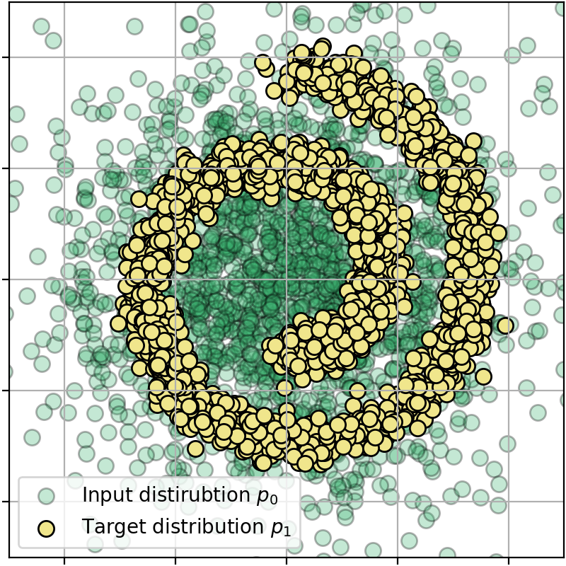
(a) ${x\sim p_{0}}$, ${y\sim p_{1}}.$

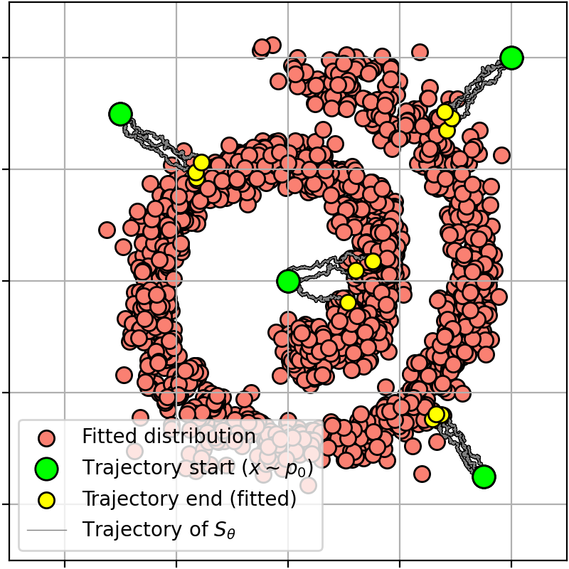
(b) $\epsilon=0.01$.

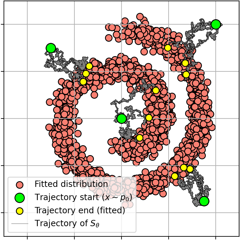
(c) $\epsilon=0.1$.

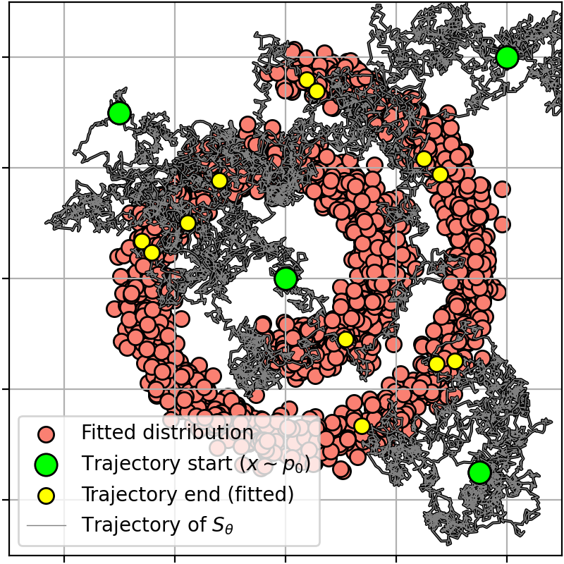
(d) $\epsilon=1$.

Figure 1: The process $S_{\theta}$ learned with LightSB-M (ours) in Gaussian $\!\rightarrow\!$ Swiss roll example (5.1).

		$\epsilon=0.1$				$\epsilon=1$				$\epsilon=10$
	Solver Type	$D\!=\!2$	$D\!=\!16$	$D\!=\!64$	$D\!=\!128$	$D\!=\!2$	$D\!=\!16$	$D\!=\!64$	$D\!=\!128$	$D\!=\!2$	$D\!=\!16$	$D\!=\!64$	$D\!=\!128$
Best solver on benchmark†	Varies	$1.94$	$13.67$	$11.74$	$11.4$	$1.04$	$9.08$	$18.05$	$15.23$	$1.40$	$1.27$	$2.36$	$1.31$
LightSB†	KL minimization	$0.03$	$0.08$	$0.28$	$0.60$	$0.05$	$0.09$	$0.24$	$0.62$	$0.07$	$0.11$	$0.21$	$0.37$
DSBM	Bridge matching	$5.2$	$16.8$	$37.3$	$35$	$0.3$	$1.1$	$9.7$	$31$	$3.7$	$105$	$3557$	$15000$
$\text{SF}^{2}$M-Sink		$0.54$	$3.7$	$9.5$	$10.9$	$0.2$	$1.1$	$9$	$23$	$0.31$	$4.9$	$319$	$819$
LightSB-M (ID, ours)		$0.04$	$0.18$	$0.77$	$1.66$	$0.09$	$\mathbf{0.18}$	$0.47$	$1.2$	$\mathbf{0.12}$	$0.19$	$\mathbf{0.36}$	$0.71$
LightSB-M (MB, ours)		$\mathbf{0.02}$	$\mathbf{0.1}$	$0.56$	$1.32$	$0.09$	$\mathbf{0.18}$	$\mathbf{0.46}$	$\mathbf{1.2}$	$0.13$	$\mathbf{0.18}$	$\mathbf{0.36}$	$0.71$
LightSB-M (GT, ours)		$\mathbf{0.02}$	$\mathbf{0.1}$	$\mathbf{0.49}$	$\mathbf{1.16}$	$\mathbf{0.09}$	$\mathbf{0.18}$	$0.47$	$\mathbf{1.2}$	$0.13$	$\mathbf{0.18}$	$\mathbf{0.36}$	$\mathbf{0.69}$

Table 1: Comparisons of $\text{cB}\mathbb{W}_{2}^{2}\text{-UVP}\downarrow$ (%) between the optimal plan $\pi^{*}$ and the learned plan $\pi_{\theta}$ on the EOT/SB benchmark (5.2).
The best metric over bridge matching solvers is bolded. Results marked with $\dagger$ are taken from (Korotin et al., 2024).

Solver type		50	100	1000
Langevin-based	(Mokrov et al., 2024)† [1 GPU V100]	$2.39\pm 0.06$ ($19$ m)	$2.32\pm 0.15$ ($19$ m)	$1.46\pm 0.20$ ($15$ m)
Minimax	(Gushchin et al., 2023a)† [1 GPU V100]	$2.44\pm 0.13$ ($43$ m)	$2.24\pm 0.13$ ($45$ m)	$1.32\pm 0.06$ ($71$ m)
IPF	(Vargas et al., 2021)† [1 GPU V100]	$3.14\pm 0.27$ ($8$ m)	$2.86\pm 0.26$ ($8$ m)	$2.05\pm 0.19$ ($11$ m)
KL minimization	LightSB (Korotin et al., 2024)† [4 CPU cores]	$2.31\pm 0.27$ ($65$ s)	$2.16\pm 0.26$ ($66$ s)	$1.27\pm 0.19$ ($146$ s)
Bridge matching	DSBM (Shi et al., 2023) [1 GPU V100]	$2.46\pm 0.1$ ($6.6$ m)	$2.35\pm 0.1$ ($6.6$ m)	$1.36\pm 0.04$ ($8.9$ m)
	$\text{SF}^{2}$M-Sink (Tong et al., 2023) [1 GPU V100]	$2.66\pm 0.18$ ($8.4$ m)	$2.52\pm 0.17$ ($8.4$ m)	$1.38\pm 0.05$ ($13.8$ m)
	LightSB-M (ID, ours) [4 CPU cores]	$2.347\pm 0.11$ ($58$ s)	$2.174\pm 0.08$ ($60$ s)	$1.35\pm 0.05$ ($147$ s)
	LightSB-M (MB, ours) [4 CPU cores]	$\mathbf{2.33}\pm 0.09$ ($80$ s)	$\mathbf{2.172}\pm 0.08$ ($80$ s)	$\mathbf{1.33}\pm 0.05$ ($176$ s)

Table 2: Energy distance (averaged for two setups and 5 random seeds) on the MSCI dataset (5.3) along with $95\%$-confidence interval ($\pm$ intervals) and average training times (s - seconds, m - minutes). The best bridge matching solver according to the mean value is bolded. Results marked with $\dagger$ are taken from (Korotin et al., 2024).

5 Experimental Illustrations

To evaluate our new LightSB-M solver, we considered several setups from related works. The code for our solver, and all experiments with it is written in Pytorch and is avaliabile in the supplementary materials. For each experiment we present a separate self-explaining Jupyter notebook, which can be used to reproduce the results of our solver. We provide the technical details in Appendix B.

5.1 Qualitative 2D Example

We start our evaluation with an illustrative 2D setup. We solve the SB between a Gaussian distribution $p_{0}$ and a Swiss roll $p_{1}$. We run our LightSB-M solver with mini-batch (MB) discrete OT as plan $\pi$ for different values of the coefficient $\epsilon$ and present the results in Figure 1. As expected, we see that the amount of noise in the trajectories and the stochasticity of the learned map are proportional to coefficient $\epsilon$.

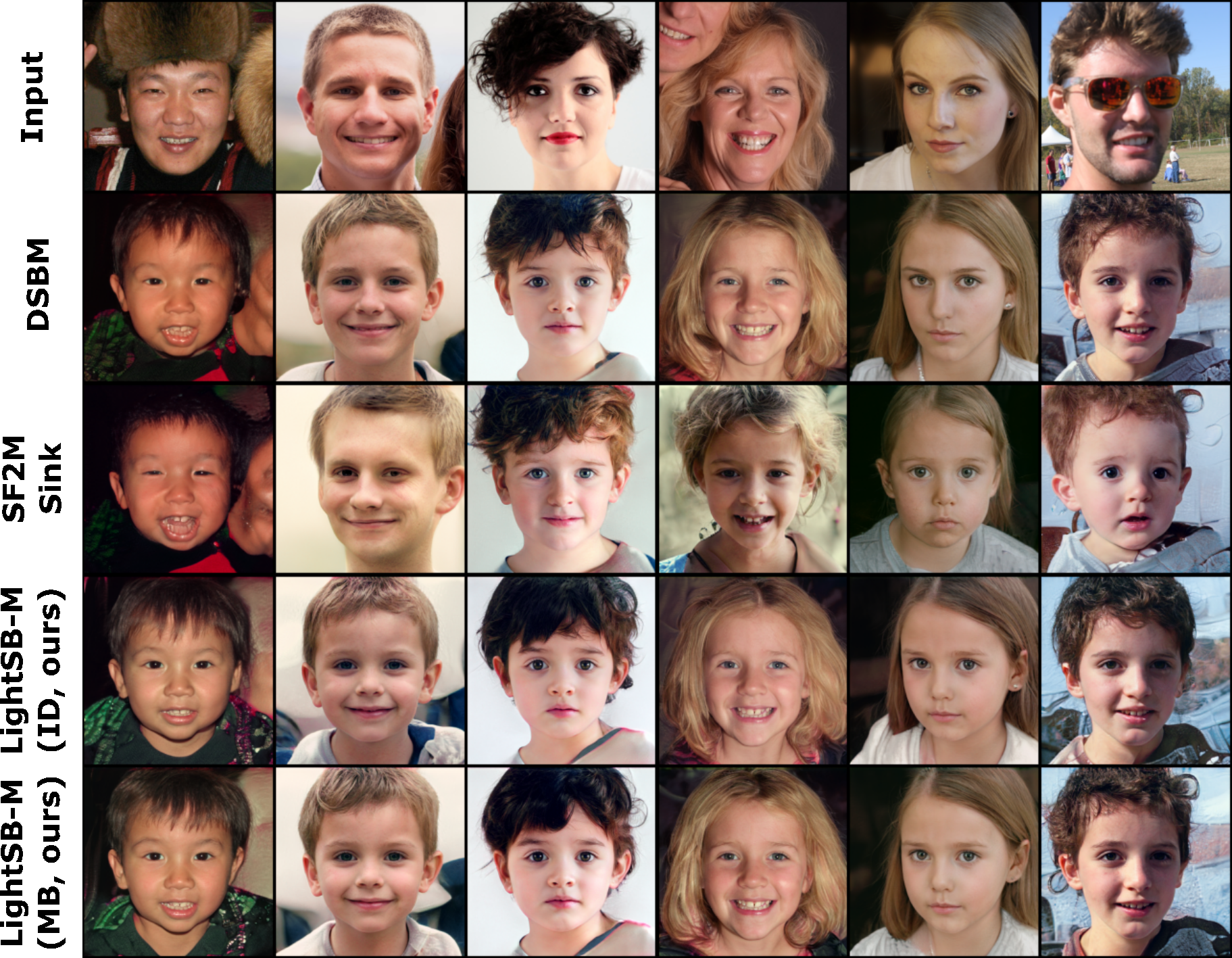
(a) Adult $\rightarrow$ Child

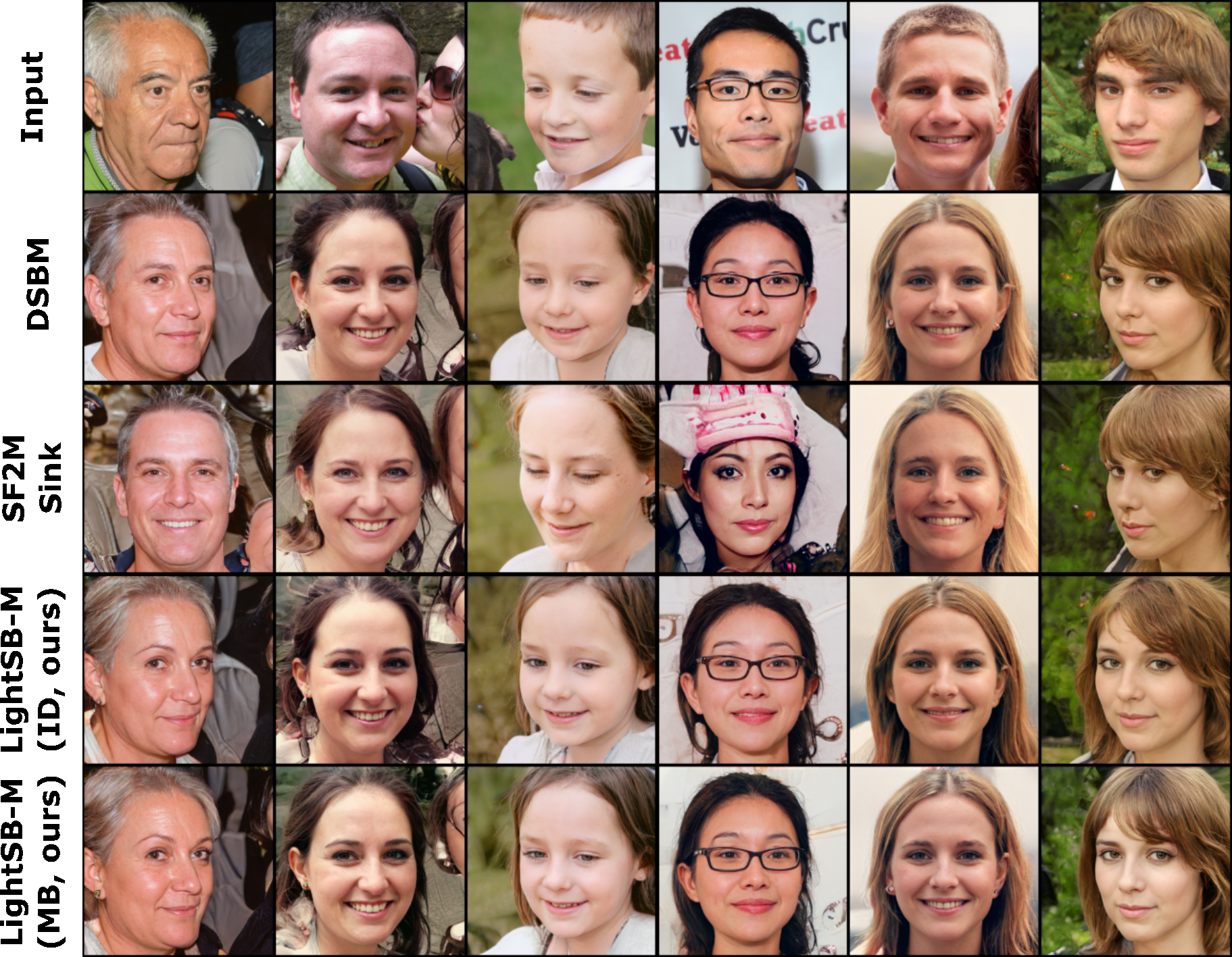
(b) Man $\rightarrow$ Woman

Figure 2: Unpaired translation between subsets of FFHQ dataset (1024x1024) performed by various SB solvers (5.4).

5.2 Quantitative Evaluation on the SB Benchmark

We use the SB mixtures benchmark proposed by (Gushchin et al., 2023b, 4) to experimentally verify that our approach based on the optimal projection is indeed able to solve the Schrödinger Bridge between $p_{0}$ and $p_{1}$ by using any reciprocal process $T_{\pi}$, $\pi\in\Pi(p_{0},p_{1})$. The benchmark provides continuous probability distribution pairs $p_{0},p_{1}$ for dimensions $D\in\{2,16,64,128\}$ with the known EOT plan $\pi^{*}(x_{0},x_{1})$ for parameter $\epsilon\in\{0.1,1.10\}$. To evaluate the quality of the SB solution (EOT plan) we use $\text{cB}\mathbb{W}_{2}^{2}\text{-UVP}$ metric as suggested by the authors (Gushchin et al., 2023b, 5). Additionally, we study how well the solvers restore the target distribution $p_{1}$ in Appendix B.3.

We provide results of our LightSB-M solver with independent (ID) and mini-batch discrete OT (MB) as $\pi$ in $T_{\pi}$ for mixture benchmark pairs in Table 1. Since the benchmark provides the ground truth EOT plan $\pi^{*}$ (GT), we also run our solver with it. Note that we have access to the GT EOT plan thanks to the benchmark, and in regular setups there is, of course, no access to it. As shown in the Table 1, our solver demonstrates comparable performance to the best among other solvers for all considered plans $\pi$.

We empirically see that our LightSB-M solver finds the same (optimal) solution for all considered plans $\pi$.

Baselines. We present results for other bridge matching methods such as DSBM (Shi et al., 2023), which uses Markovian and reciprocal projections, and $\text{SF}^{2}$M-Sink (Tong et al., 2023), which uses an approximation of the EOT plan by the Sinkhorn algorithm (Cuturi, 2013). On the setups with $\epsilon=10$ both methods exibits difficulties due to the necessity to learn SDE with high magnitude. On the setups with $\epsilon=0.1$ and $\epsilon=1$, $\text{SF}^{2}$M-Sink works better than DSBM. This result may seem counterintuitive at first, since DSBM methods should find the true SB solution, while $\text{SF}^{2}$M-Sink should find some approximation to it based on how close the minibatch discrete EOT approximates the GT EOT plan. One possible reason is that DSBM simply requires more iterations of Markovian/reciprocal projections. However, in our experiments we observe that increasing the number of iterations does not improve the quality.

5.3 Quantitative Evaluation on Biological Data

We evaluate our algorithm on the inference of cell trajectories from unpaired single-cell data problem, where OT/SB is widely used (Vargas et al., 2021; Tong et al., 2023; Koshizuka & Sato, 2022). We consider the recent high-dimensional single-cell setup provided by (Tong et al., 2023) based on the dataset from the Kaggle competition ”Open Problems - Multimodal Single-Cell Integration.” This dataset provides single-cell data from four human donors on days $2,3,4$ and $7$ and describes the gene expression levels of distinct cells. The task of this setup is to learn a trajectory model for the cell dynamics, given only unpaired samples at two time points, representing distributions $p_{0}$ and $p_{1}$. As in related works (Tong et al., 2023; Korotin et al., 2024), we use PCA projections of the original data with $\text{DIM}\in\{50,100,1000\}$ components.

In our experiments, we consider two setups by taking data from two different days as $p_{0},p_{1}$ to solve the Shrödinger Bridge and one intermediate day for evaluation. The first setup includes data from day 2 as $p_{0}$, data from day $4$ as $p_{1}$, and data from day $3$ for evaluation, while the second setup includes data from day $3$ as $p_{0}$, data from day $7$ as $p_{1}$, and data from day $4$ for evaluation. At evaluation, we use learned models to sample one trajectory for each cell from the initial distribution $p_{0}$ and then compare the predicted distribution at the intermediate time point with the ground truth data distribution. For comparison, we use energy distance (Rizzo & Székely, 2016) and present results in Table 2.

We see that our LightSB-M’s solution with independent (ID) and minibatch discrete OT (MB) plans for $T_{\pi}$ provides the same metrics since it learns the same solution, as follows from the developed theory. It also shows performance on the same level as other neural network-based matching methods such as DSBM and $\text{SF}^{2}$M-Sink, but converges faster even without using GPU similar to the LightSB solver.

5.4 Comparison on Unpaired Image-to-image Transfer

Another popular setup that involves learning a translation between two distributions without paired data is image-to-image translation (Zhu et al., 2017). Methods based on SB show promising results in solving this problem thanks to the perfect theoretical agreement of this setup with the SB formulation (Shi et al., 2023). Due to the used parameterization based on Gaussian mixture, learning the translation between low-dimensional image manifolds is difficult for LightSB-M. Fortunately, many approaches use autoencoders (Rombach et al., 2022) for more efficient generation and translation. We follow the setup of (Korotin et al., 2024) with the pre-trained ALAE autoencoder (Pidhorskyi et al., 2020) on $1024\times 1024$ FFHQ dataset (Karras et al., 2019).

We present the qualitative results of our solver with discrete minibatch OT plan (MB) and independent plan (ID) in Fig 2. For comparison, we also provide results of DSBM and $\text{SF}^{2}$M-Sink. Our LightSB-M solver converges to nearly the same solution for both ID and MB plans and demonstrates good results. The samples provided by DSBM are close to the samples of LightSB-M, which is expected since both methods provide theoretical guarantees for solving the SB problem. Samples obtained by $\text{SF}^{2}$M-Sink slightly differ, probably due to the bias of the discrete EOT plans. We provide additional examples of translation in Appendix B.5.

6 Discussion

Potential impact. Our main contribution is methodological: we show that one may perform just a single (but optimal) bridge matching step to learn SB. This finding helps us eliminate limitations of existing bridge matching-based approaches, such as heuristical minibatch OT approximations or error accumulation during training. We believe that this insight is a significant step towards developing novel efficient computational approaches for SB/EOT tasks.

Limitations are discussed in Appendix C.

7 Broader impact

This paper presents work whose goal is to advance the field of Machine Learning. There are many potential societal consequences of our work, none which we feel must be specifically highlighted here.

8 ACKNOWLEDGEMENTS

The work was supported by the Analytical center under the RF Government (subsidy agreement 000000D730321P5Q0002, Grant No. 70-2021-00145 02.11.2021).

Appendix A Proofs

Proof of Theorem 3.1.

Let $p_{0},p_{1}$ denote the marginals of $\pi$. Let $\pi^{*}$ be the EOT plan between $p_{0},p_{1}$. Let $p^{S}_{0},p^{S}_{1}$ denote the distribution of $S$ at $t=0$ and $t=1$, respectively. We use the fact that each element $S$ of $\mathcal{S}$ is a reciprocal process with some EOT plan $\pi^{S}\in\Pi(p_{0}^{S},p_{1}^{S})$, i.e. $S=\int W^{\epsilon}_{|x_{0},x_{1}}d\pi^{S}(x_{0},x_{1})$, recall 2.1. In turn, $\pi^{S}$ can be represented through the input density $p^{S}_{0}$ and the potential $v^{S}$ as in (6), i.e.:

$$\pi^{S}(x_{0},x_{1})=p^{S}_{0}(x_{0})\frac{\exp\big{(}\nicefrac{{\langle x_{0},x_{1}\rangle}}{{\epsilon}}\big{)}v^{S}(x_{1})}{c_{v^{S}}(x_{0})}$$ (16)

We derive:

$$\text{KL}\left(T_{\pi}\|S\right)=\text{KL}\left(\pi\|\pi^{S}\right)+\int_{\mathbb{R}^{D}\times\mathbb{R}^{D}}\text{KL}\left(T_{\pi|x_{0},x_{1}}\|S_{|x_{0},x_{1}}\right)\pi(x_{0},x_{1})dx_{0}dx_{1}=$$ (17)

$$\text{KL}\left(\pi\|\pi^{S}\right)+\int_{\mathbb{R}^{D}\times\mathbb{R}^{D}}\underbrace{\text{KL}\left(W^{\epsilon}_{|x_{0},x_{1}}\|W^{\epsilon}_{|x_{0},x_{1}}\right)}_{=0}\pi(x_{0},x_{1})dx_{0}dx_{1}=$$ (18)

$$\int_{\mathbb{R}^{D}\times\mathbb{R}^{D}}\frac{\log\pi(x_{0},x_{1})}{\log\pi^{S}(x_{0},x_{1})}\pi(x_{0},x_{1})dx_{0}dx_{1}=$$

$$\int_{\mathbb{R}^{D}\times\mathbb{R}^{D}}\log\pi(x_{0},x_{1})\pi(x_{0},x_{1})dx_{0}dx_{1}-\int_{\mathbb{R}^{D}\times\mathbb{R}^{D}}\log\pi^{S}(x_{0},x_{1})\pi(x_{0},x_{1})dx_{0}dx_{1}=$$

$$-H(\pi)-\int_{\mathbb{R}^{D}\times\mathbb{R}^{D}}\log\pi^{S}(x_{0},x_{1})\pi(x_{0},x_{1})dx_{0}dx_{1}=$$ (19)

$$-H(\pi)-\int_{\mathbb{R}^{D}\times\mathbb{R}^{D}}\log\Big{(}p_{0}^{S}(x_{0})\frac{\exp\Big{(}\nicefrac{{\langle x_{0},x_{1}\rangle}}{{\epsilon}}\Big{)}v^{S}(x_{1})}{c_{v^{S}}(x_{0})}\Big{)}\pi(x_{0},x_{1})dx_{0}dx_{1}=$$ (20)

$$-H(\pi)-\int_{\mathbb{R}^{D}\times\mathbb{R}^{D}}\Big{(}\log p_{0}^{S}(x_{0})+\langle x_{0},x_{1}\rangle+\log v^{S}(x_{1})-\log c_{v^{S}}(x_{0})\Big{)}\pi(x_{0},x_{1})dx_{0}dx_{1}=$$

$$-H(\pi)-\int_{\mathbb{R}^{D}\times\mathbb{R}^{D}}\langle x_{0},x_{1}\rangle\pi(x_{0},x_{1})dx_{0}dx_{1}$$

$$-\int_{\mathbb{R}^{D}\times\mathbb{R}^{D}}\Big{(}\log p_{0}^{S}(x_{0})-\log c_{v^{S}}(x_{0})\Big{)}\pi(x_{0},x_{1})dx_{0}dx_{1}-\int_{\mathbb{R}^{D}\times\mathbb{R}^{D}}\log v^{S}(x_{1})\pi(x_{0},x_{1})dx_{0}dx_{1}=$$

$$-H(\pi)-\int_{\mathbb{R}^{D}\times\mathbb{R}^{D}}\langle x_{0},x_{1}\rangle\pi(x_{0},x_{1})dx_{0}dx_{1}$$

$$-\int_{\mathbb{R}^{D}}\big{\{}(\log p_{0}^{S}(x_{0})-\log c_{v^{S}}(x_{0}))\underbrace{\int_{\mathbb{R}^{D}}\pi(x_{1}|x_{0})dx_{1}}_{=1=\int_{\mathbb{R}^{D}}\pi^{*}(x_{1}|x_{0})dx_{1}}\big{\}}\underbrace{\pi(x_{0})}_{=\pi^{*}(x_{0})}dx_{0}-\int_{\mathbb{R}^{D}}\log v^{S}(x_{1})\underbrace{\big{(}\int_{\mathbb{R}^{D}}\pi(x_{0}|x_{1})dx_{0}\big{)}}_{=1=\int_{\mathbb{R}^{D}}\pi^{*}(x_{0}|x_{1})dx_{0}}\underbrace{\pi(x_{1})}_{=\pi^{*}(x_{1})}dx_{1}=$$

$$-H(\pi)-\int_{\mathbb{R}^{D}\times\mathbb{R}^{D}}\langle x_{0},x_{1}\rangle\pi(x_{0},x_{1})dx_{0}dx_{1}$$

$$-\int_{\mathbb{R}^{D}}\big{\{}(\log p_{0}^{S}(x_{0})-\log c_{v^{S}}(x_{0}))\int_{\mathbb{R}^{D}}\pi^{*}(x_{1}|x_{0})dx_{1}\big{\}}\pi^{*}(x_{0})dx_{0}-\int_{\mathbb{R}^{D}}\log v^{S}(x_{1})\big{(}\int_{\mathbb{R}^{D}}\pi^{*}(x_{0}|x_{1})dx_{0}\big{)}\pi^{*}(x_{1})dx_{1}=$$

$$-H(\pi)-\int_{\mathbb{R}^{D}\times\mathbb{R}^{D}}\langle x_{0},x_{1}\rangle\pi(x_{0},x_{1})dx_{0}dx_{1}$$

$$-\int_{\mathbb{R}^{D}\times\mathbb{R}^{D}}\Big{(}\log p_{0}^{S}(x_{0})-\log c_{v^{S}}(x_{0})\Big{)}\pi^{*}(x_{0},x_{1})dx_{0}dx_{1}-\int_{\mathbb{R}^{D}\times\mathbb{R}^{D}}\log v^{S}(x_{1})\pi^{*}(x_{0},x_{1})dx_{0}dx_{1}=$$

$$-H(\pi)-\int_{\mathbb{R}^{D}\times\mathbb{R}^{D}}\langle x_{0},x_{1}\rangle\pi(x_{0},x_{1})dx_{0}dx_{1}+\underbrace{\int_{\mathbb{R}^{D}\times\mathbb{R}^{D}}\langle x_{0},x_{1}\rangle\pi^{*}(x_{0},x_{1})dx_{0}dx_{1}-\int_{\mathbb{R}^{D}\times\mathbb{R}^{D}}\langle x_{0},x_{1}\rangle\pi^{*}(x_{0},x_{1})dx_{0}dx_{1}}_{=0}$$

$$-\int_{\mathbb{R}^{D}\times\mathbb{R}^{D}}\Big{(}\log p_{0}^{S}(x_{0})+\log v^{S}(x_{1})-\log c_{v^{S}}(x_{0})\Big{)}\pi^{*}(x_{0},x_{1})dx_{0}dx_{1}=$$

$$-H(\pi)-\int_{\mathbb{R}^{D}\times\mathbb{R}^{D}}\langle x_{0},x_{1}\rangle\pi(x_{0},x_{1})dx_{0}dx_{1}+\int_{\mathbb{R}^{D}\times\mathbb{R}^{D}}\langle x_{0},x_{1}\rangle\pi^{*}(x_{0},x_{1})dx_{0}dx_{1}$$

$$-\int_{\mathbb{R}^{D}\times\mathbb{R}^{D}}\Big{(}\log p_{0}^{S}(x_{0})+\langle x_{0},x_{1}\rangle+\log v^{S}(x_{1})-\log c_{v^{S}}(x_{0})\Big{)}\pi^{*}(x_{0},x_{1})dx_{0}dx_{1}=$$

$$-H(\pi)-\int_{\mathbb{R}^{D}\times\mathbb{R}^{D}}\langle x_{0},x_{1}\rangle\pi(x_{0},x_{1})dx_{0}dx_{1}+\int_{\mathbb{R}^{D}\times\mathbb{R}^{D}}\langle x_{0},x_{1}\rangle\pi^{*}(x_{0},x_{1})dx_{0}dx_{1}$$

$$-\int_{\mathbb{R}^{D}\times\mathbb{R}^{D}}\log\Big{(}p_{0}^{S}(x_{0})\underbrace{\frac{\exp\Big{(}\nicefrac{{\langle x_{0},x_{1}\rangle}}{{\epsilon}}\Big{)}v^{S}(x_{1})}{c_{v^{S}}(x_{0})}}_{\pi^{S}(x_{1}|x_{0})}\Big{)}\pi^{*}(x_{0},x_{1})dx_{0}dx_{1}=$$

$$-H(\pi)-\int_{\mathbb{R}^{D}\times\mathbb{R}^{D}}\langle x_{0},x_{1}\rangle(\pi(x_{0},x_{1})-\pi^{*}(x_{0},x_{1}))dx_{0}dx_{1}-\int_{\mathbb{R}^{D}\times\mathbb{R}^{D}}\log\pi^{S}(x_{0},x_{1})\pi^{*}(x_{0},x_{1})dx_{0}dx_{1}$$

$$+\underbrace{\int_{\mathbb{R}^{D}\times\mathbb{R}^{D}}\log\pi^{*}(x_{0},x_{1})\pi^{*}(x_{0},x_{1})dx_{0}dx_{1}-\int_{\mathbb{R}^{D}\times\mathbb{R}^{D}}\log\pi^{*}(x_{0},x_{1})\pi^{*}(x_{0},x_{1})dx_{0}dx_{1}}_{=0}=$$

$$\underbrace{-H(\pi)-\int_{\mathbb{R}^{D}\times\mathbb{R}^{D}}\langle x_{0},x_{1}\rangle(\pi(x_{0},x_{1})-\pi^{*}(x_{0},x_{1}))dx_{0}dx_{1}-\int_{\mathbb{R}^{D}\times\mathbb{R}^{D}}\log\pi^{*}(x_{0},x_{1})\pi^{*}(x_{0},x_{1})dx_{0}dx_{1}}_{\stackrel{{\scriptstyle\text{def}}}{{=}}\widehat{C}(\pi)}$$

$$+\underbrace{\int_{\mathbb{R}^{D}\times\mathbb{R}^{D}}\log\frac{\pi^{*}(x_{0},x_{1})}{\pi^{S}(x_{0},x_{1})}\pi^{*}(x_{0},x_{1})dx_{0}dx_{1}}_{=\text{KL}\left(\pi^{*}\|\pi^{S}\right)}=$$

$$\widehat{C}(\pi)+\text{KL}\left(\pi^{*}\|\pi^{S}\right).$$

In (17) we use disintegration theorem for KL divergence to distinguish process plan $\pi^{S}$ and ”inner part” (Vargas et al., 2021, Appendix C, D). In transition from (17) to (18) we notice, that $T_{\pi|x_{0},x_{1}}=W^{\epsilon}_{|x_{0},x_{1}}$ and $S_{|x_{0},x_{1}}=W^{\epsilon}_{|x_{0},x_{1}}$, since $T_{\pi}$ is a reciprocal process as well as Schrödinger Bridge $S$. In transition from (19) to (20) we use the fact, that $\pi^{S}$ is given by (16). Since

$$\text{KL}\left(T_{\pi}\|S\right)=\widehat{C}(\pi)+\text{KL}\left(\pi^{*}\|\pi^{S}\right),$$

the minimum of $\text{KL}\left(T_{\pi}\|S\right)$ is achieved for $S$ such that $\pi^{S}=\pi^{*}$, i.e., when $S$ is the SB between $p_{0}$ and $p_{1}$.

∎

Proof of Theorem 3.2.

We start by using a Pythagorean theorem for Markovian projection (Shi et al., 2023, Lemma 6)

$$\text{KL}\left(T_{\pi}\|S_{v}\right)=\text{KL}\left(T_{\pi}\|\text{proj}_{\mathcal{M}}(T_{\pi})\right)+\text{KL}\left(\text{proj}_{\mathcal{M}}(T_{\pi})\|S_{v}\right),$$ (21)

where the drift $g_{\mathcal{M}}$ of the Markoian projection $\text{proj}_{\mathcal{M}}(T_{\pi})$ is given by (9):

$$g_{\mathcal{M}}(x_{t},t)=\int_{\mathbb{R}^{D}}\frac{x_{1}-x_{t}}{1-t}dp_{T_{\pi}}(x_{1}|x_{t}).$$ (22)

We use the expression of KL between Markovian processes starting from the same distribution $p_{0}$ through their drifts (Pavon & Wakolbinger, 1991) and note that Markovian projection preserve the time marginals $p_{T_{\pi}}(x_{t})$:

$$\text{KL}\left(\text{proj}_{\mathcal{M}}(T_{\pi})\|S_{v}\right)=\frac{1}{2\epsilon}\int_{0}^{1}\int_{\mathbb{R}^{D}}||g_{v}(x_{t},t)-g_{\mathcal{M}}(x_{t},t)||^{2}dp_{T_{\pi}}(x_{t})dt$$ (23)

Then we substitute $g_{\mathcal{M}}$ by (22):

$$\text{KL}\left(\text{proj}_{\mathcal{M}}(T_{\pi})\|S_{v}\right)=\frac{1}{2\epsilon}\int_{0}^{1}\int_{\mathbb{R}^{D}}||g_{v}(x_{t},t)-g_{\mathcal{M}}(x_{t},t)||^{2}dp_{T_{\pi}}(x_{t})dt=$$

$$\frac{1}{2\epsilon}\int_{0}^{1}\int_{\mathbb{R}^{D}}||g_{v}(x_{t},t)-\int_{\mathbb{R}^{D}}\frac{x_{1}-x_{t}}{1-t}dp_{T_{\pi}}(x_{1}|x_{t})||^{2}dp_{T_{\pi}}(x_{t})dt=$$

$$\frac{1}{2\epsilon}\int_{0}^{1}\int_{\mathbb{R}^{D}}\Big{\{}||g_{v}(x_{t},t)||^{2}-2\langle g_{v}(x_{t},t),\int_{\mathbb{R}^{D}}\frac{x_{1}-x_{t}}{1-t}dp_{T_{\pi}}(x_{1}|x_{t})\rangle\Big{\}}dp_{T_{\pi}}(x_{t})dt+$$

$$\underbrace{\frac{1}{2\epsilon}\int_{0}^{1}\int_{\mathbb{R}^{D}}||\int_{\mathbb{R}^{D}}\frac{x_{1}-x_{t}}{1-t}dp_{T_{\pi}}(x_{1}|x_{t})||^{2}dp_{T_{\pi}}(x_{t})dt}_{\stackrel{{\scriptstyle\text{def}}}{{=}}C^{\prime}(\pi)}=$$

$$\frac{1}{2\epsilon}\int_{0}^{1}\int_{\mathbb{R}^{D}}\Big{\{}||g_{v}(x_{t},t)||^{2}-2\langle g_{v}(x_{t},t),\int_{\mathbb{R}^{D}}\frac{x_{1}-x_{t}}{1-t}dp_{T_{\pi}}(x_{1}|x_{t})\rangle\Big{\}}dp_{T_{\pi}}(x_{t})dt+C^{\prime}(\pi)=$$

$$\frac{1}{2\epsilon}\int_{0}^{1}\int_{\mathbb{R}^{D}}\int_{\mathbb{R}^{D}}\Big{\{}||g_{v}(x_{t},t)||^{2}-2\langle g_{v}(x_{t},t),\frac{x_{1}-x_{t}}{1-t}\rangle\Big{\}}\underbrace{dp_{T_{\pi}}(x_{1}|x_{t})dp_{T_{\pi}}(x_{t})}_{dp_{T_{\pi}}(x_{t},x_{1})}dt+C^{\prime}(\pi)=$$

$$\frac{1}{2\epsilon}\int_{0}^{1}\int_{\mathbb{R}^{D}}\int_{\mathbb{R}^{D}}\Big{\{}||g_{v}(x_{t},t)||^{2}-2\langle g_{v}(x_{t},t),\frac{x_{1}-x_{t}}{1-t}\rangle\Big{\}}dp_{T_{\pi}}(x_{t},x_{1})dt+C^{\prime}(\pi)=$$

$$\frac{1}{2\epsilon}\int_{0}^{1}\int_{\mathbb{R}^{D}}\int_{\mathbb{R}^{D}}\Big{\{}||g_{v}(x_{t},t)-\frac{x_{1}-x_{t}}{1-t}||^{2}\Big{\}}dp_{T_{\pi}}(x_{t},x_{1})dt-$$

$$\underbrace{\frac{1}{2\epsilon}\int_{0}^{1}\int_{\mathbb{R}^{D}}\int_{\mathbb{R}^{D}}||\frac{x_{1}-x_{t}}{1-t}||^{2}dp_{T_{\pi}}(x_{t},x_{1})dt+C^{\prime}(\pi)}_{\stackrel{{\scriptstyle\text{def}}}{{=}}C^{\prime\prime}(\pi)}=$$

$$\frac{1}{2\epsilon}\int_{0}^{1}\int_{\mathbb{R}^{D}}\int_{\mathbb{R}^{D}}\Big{\{}||g_{v}(x_{t},t)-\frac{x_{1}-x_{t}}{1-t}||^{2}\Big{\}}dp_{T_{\pi}}(x_{t},x_{1})dt+C^{\prime\prime}(\pi)$$

Thus,

$$\text{KL}\left(T_{\pi}\|S_{v}\right)=\underbrace{\text{KL}\left(T_{\pi}\|\text{proj}_{\mathcal{M}}(T_{\pi})\right)+C^{\prime}(T_{\pi})}_{\stackrel{{\scriptstyle\text{def}}}{{=}}C(\pi)}+$$

$$\frac{1}{2\epsilon}\int_{0}^{1}\int_{\mathbb{R}^{D}}\int_{\mathbb{R}^{D}}\Big{\{}||g_{v}(x_{t},t)-\frac{x_{1}-x_{t}}{1-t}||^{2}\Big{\}}dp_{T_{\pi}}(x_{t},x_{1})dt=$$

$$C(\pi)+\frac{1}{2\epsilon}\int_{0}^{1}\int_{\mathbb{R}^{D}}\int_{\mathbb{R}^{D}}\Big{\{}||g_{v}(x_{t},t)-\frac{x_{1}-x_{t}}{1-t}||^{2}\Big{\}}dp_{T_{\pi}}(x_{t},x_{1})dt.$$ (24)

∎

Proof of Theorem 3.3.

From Theorem 3.2 it follows that:

$$\text{KL}\left(T_{\pi}\|S_{v}\right)=C(\pi)+\frac{1}{2\epsilon}\int_{0}^{1}\int_{\mathbb{R}^{D}}\int_{\mathbb{R}^{D}}\Big{\{}||g_{v}(x_{t},t)-\frac{x_{1}-x_{t}}{1-t}||^{2}\Big{\}}dp_{T_{\pi}}(x_{t},x_{1})dt.$$ (25)

In turn, from the proof of Theorem (3.1) it holds that:

$$\text{KL}\left(T_{\pi}\|S_{v}\right)=\widehat{C}(\pi)+\text{KL}\left(\pi^{*}\|\pi^{S_{v}}\right).$$ (26)

From the (Korotin et al., 2024, Propositon 3.1) it follows that $\text{KL}\left(\pi^{*}\|\pi^{S}_{v}\right)=\mathcal{L}_{0}(v)-\mathcal{L}^{*}$, where $\mathcal{L}^{*}$ is a constant depending on distirbutions $p_{0},p_{1}$ and value $\epsilon$. Hence, we combine these two expressions and get

$$\frac{1}{2\epsilon}\int_{0}^{1}\int_{\mathbb{R}^{D}}\int_{\mathbb{R}^{D}}\Big{\{}||g_{v}(x_{t},t)-\frac{x_{1}-x_{t}}{1-t}||^{2}\Big{\}}dp_{T_{\pi}}(x_{t},x_{1})dt=\widetilde{C}(\pi)+\mathcal{L}_{0}(v),$$

where $\widetilde{C}(\pi)\stackrel{{\scriptstyle\text{def}}}{{=}}\widehat{C}(\pi)-\mathcal{L}^{*}-C(\pi)$.

∎

Appendix B Experiments details

B.1 General Implementation Details

We build our LightSB-M implementation upon LightSB official implementation https://github.com/ngushchin/LightSB. All the parametrization, optimization and initialization details are the same as (Korotin et al., 2024) if not stated otherwise. In the Mini-batch (MB) setting, discrete OT algorithm ot.emd is taken from POT library (Flamary et al., 2021). The batch size is always 128.

B.2 Qualitative 2D setup

We use $K=250$ potentials and Adam optimizer with $lr=10^{-3}$ in all the cases to train LightSB-M.

B.3 Quantitative Evaluation on the SB Benchmark

Target metrics. We additionally study how well each solver map initial distribution $p_{0}$ into $p_{1}$ by measuring the metric $\text{B}\mathbb{W}_{2}^{2}\text{-UVP}$ also proposed by the aurhos of the benchmark (Gushchin et al., 2023b, 4). We present the results in Table 3.

		$\epsilon=0.1$				$\epsilon=1$				$\epsilon=10$
	Solver Type	$D\!=\!2$	$D\!=\!16$	$D\!=\!64$	$D\!=\!128$	$D\!=\!2$	$D\!=\!16$	$D\!=\!64$	$D\!=\!128$	$D\!=\!2$	$D\!=\!16$	$D\!=\!64$	$D\!=\!128$
Best solver on benchmark†	Varies	$0.016$	$0.05$	$0.25$	$0.22$	$0.005$	$0.09$	$0.56$	$0.12$	$0.01$	$0.02$	$0.15$	$0.23$
LightSB†	KL minimization	$0.005$	$0.017$	$0.037$	$0.069$	$0.004$	$0.01$	$0.03$	$0.07$	$0.03$	$0.04$	$0.17$	$0.30$
DSBM	Bridge matching	$0.03$	$0.18$	$0.7$	$2.26$	$0.04$	$0.09$	$1.9$	$7.3$	$0.26$	$102$	$3563$	$15000$
$\text{SF}^{2}$M-Sink		$0.04$	$0.18$	$0.39$	$1.1$	$0.07$	$0.3$	$4.5$	$17.7$	$0.17$	$4.7$	$316$	$812$
LightSB-M (ID, ours)		$0.02$	$\mathbf{0.03}$	$\mathbf{0.2}$	$\mathbf{0.46}$	$0.005$	$0.04$	$\mathbf{0.11}$	$0.27$	$0.07$	$\mathbf{0.03}$	$0.11$	$\mathbf{0.21}$
LightSB-M (MB, ours)		$\mathbf{0.005}$	$0.07$	$0.27$	$0.63$	$\mathbf{0.002}$	$0.04$	$0.12$	$0.36$	$0.04$	$0.07$	$0.11$	$0.23$
LightSB-M (GT, ours)		$0.02$	$\mathbf{0.03}$	$0.21$	$0.55$	$0.011$	$\mathbf{0.03}$	$\mathbf{0.11}$	$\mathbf{0.26}$	$\mathbf{0.016}$	$0.04$	$\mathbf{0.09}$	$\mathbf{0.21}$

Table 3: Comparisons of $\text{B}\mathbb{W}_{2}^{2}\text{-UVP}\downarrow$ (%) between the ground truth target distribution $p_{1}$ and learned target distribution $\pi_{\theta}(x_{1})$. The best metric over bridge matching solvers is bolded. Results marked with $\dagger$ are taken from (Korotin et al., 2024).

B.4 Evaluation on Biological Single-cell Data.

We follow the same setup as (Korotin et al., 2024) and use their code and data from https://github.com/ngushchin/LightSB. We train all models with $\epsilon=0.1$.

B.5 Evaluation on unpaired image-to-image translation.

We follow the same setup as (Korotin et al., 2024) and use their code and data from https://github.com/ngushchin/LightSB. We train all models with $\epsilon=0.1$.

According to (Korotin et al., 2024) we first split the FFHQ data into train (first 60k) and test (last 10k) images. Then we create subsets of males, females, children and adults in both train and test subsets. For training we first use the ALAE encoder to extract $512$ dimensional latent vectors for each image and then train our solver on the extracted latent vectors. At the inference stage, we first extract the latent vector from the image, translate it by LightSB-M, and then decode the mapped vector to produce the mapped image.

We provide additional generation examples for our LigthSB-M solver and other baselines in Figure 3.

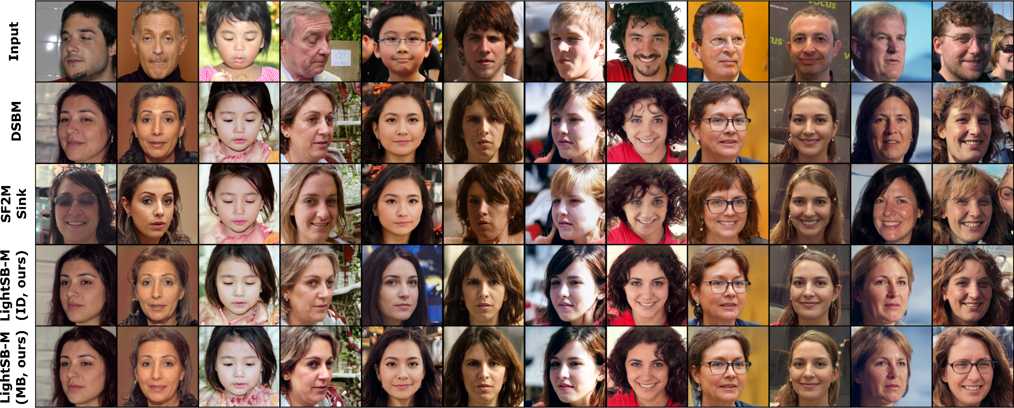
(a) Man $\rightarrow$ Woman.

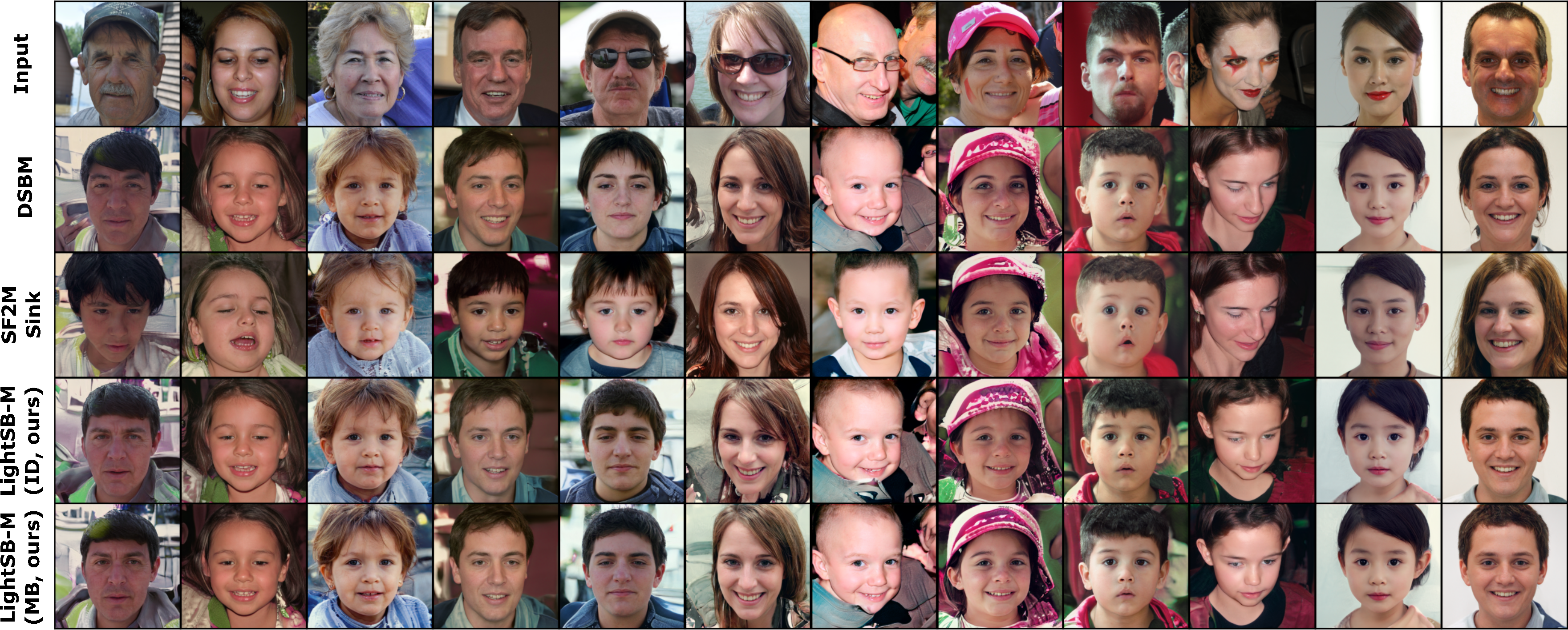
(b) Adult $\rightarrow$ Child.

Figure 3: Additional examples of image-to-image translation.

B.6 Baselines

DSBM (Shi et al., 2023). Implementation is taken from official repo

https://github.com/yuyang-shi/dsbm-pytorch

For forward and backward drift approximations, instead of those used in the official repository, we use MLP neural networks with positional encoding as they give better results. Number of inner gradient steps for Markovian Fitting Iteration is $10000$, number of Markovian Fitting Iterations is $10$. Adam optimizer (Kingma & Ba, 2014) with $lr=10^{-4}$ is used for optimization.

$\text{SF}^{2}$M-Sink (Tong et al., 2023). Implementation is taken from official repo

https://github.com/atong01/conditional-flow-matching

For drift and score function approximation, we use MLP neural networks with positional encoding instead of those used in the official repository, as they give better results. Number of gradient updates $50000$ for SB benchmark and Single-cell Data experiments and $20000$ for unpaired image-to-image translation. Adam optimizer (Kingma & Ba, 2014) with $lr=10^{-4}$ is used for optimization.

LightSB’s results are taken from the paper (Korotin et al., 2024).

Appendix C Limitations

Given a Schrödinger potential $v$, it may be not easy to compute the drift $g_{v}$ (4) of $S_{v}$ needed to perform the optimal SB matching. We employ the Gaussian mixture parameterization for $v$ for which this drift $g_{v}$ is analytically known (15). This allows to easily implement our optimal SB matching in practice and obtain a fast bridge matching based solver. Still such a parameterization sometimes may be not sufficient, e.g., for large-scale generative modeling tasks. We point to developing ways to incorporate more general parameterization of $v$ to our optimal SB matching, e.g., neural-network based, as a promising research avenue.

References

• Chen et al. (2021) Chen, T., Liu, G.-H., and Theodorou, E. A. Likelihood training of schr$\backslash$” odinger bridge using forward-backward sdes theory. arXiv preprint arXiv:2110.11291, 2021.
• Chen et al. (2016) Chen, Y., Georgiou, T. T., and Pavon, M. On the relation between optimal transport and schrödinger bridges: A stochastic control viewpoint. Journal of Optimization Theory and Applications, 169:671–691, 2016.
• Cuturi (2013) Cuturi, M. Sinkhorn distances: Lightspeed computation of optimal transport. Advances in neural information processing systems, 26, 2013.
• Daniels et al. (2021) Daniels, M., Maunu, T., and Hand, P. Score-based generative neural networks for large-scale optimal transport. Advances in neural information processing systems, 34:12955–12965, 2021.
• De Bortoli et al. (2021) De Bortoli, V., Thornton, J., Heng, J., and Doucet, A. Diffusion schrödinger bridge with applications to score-based generative modeling. Advances in Neural Information Processing Systems, 34:17695–17709, 2021.
• Dempster et al. (1977) Dempster, A. P., Laird, N. M., and Rubin, D. B. Maximum likelihood from incomplete data via the em algorithm. Journal of the royal statistical society: series B (methodological), 39(1):1–22, 1977.
• Flamary et al. (2021) Flamary, R., Courty, N., Gramfort, A., Alaya, M. Z., Boisbunon, A., Chambon, S., Chapel, L., Corenflos, A., Fatras, K., Fournier, N., Gautheron, L., Gayraud, N. T., Janati, H., Rakotomamonjy, A., Redko, I., Rolet, A., Schutz, A., Seguy, V., Sutherland, D. J., Tavenard, R., Tong, A., and Vayer, T. Pot: Python optimal transport. Journal of Machine Learning Research, 22(78):1–8, 2021. URL http://jmlr.org/papers/v22/20-451.html.
• Fortet (1940) Fortet, R. Résolution d’un système d’équations de m. schrödinger. Journal de Mathématiques Pures et Appliquées, 19(1-4):83–105, 1940.
• Genevay et al. (2016) Genevay, A., Cuturi, M., Peyré, G., and Bach, F. Stochastic optimization for large-scale optimal transport. In Advances in neural information processing systems, pp.  3440–3448, 2016.
• Genevay et al. (2019) Genevay, A., Chizat, L., Bach, F., Cuturi, M., and Peyré, G. Sample complexity of sinkhorn divergences. In The 22nd international conference on artificial intelligence and statistics, pp.  1574–1583. PMLR, 2019.
• Gushchin et al. (2023a) Gushchin, N., Kolesov, A., Korotin, A., Vetrov, D., and Burnaev, E. Entropic neural optimal transport via diffusion processes. In Advances in Neural Information Processing Systems, 2023a.
• Gushchin et al. (2023b) Gushchin, N., Kolesov, A., Mokrov, P., Karpikova, P., Spiridonov, A., Burnaev, E., and Korotin, A. Building the bridge of schr$\backslash$” odinger: A continuous entropic optimal transport benchmark. In Thirty-seventh Conference on Neural Information Processing Systems Datasets and Benchmarks Track, 2023b.
• Ho et al. (2020) Ho, J., Jain, A., and Abbeel, P. Denoising diffusion probabilistic models. Advances in neural information processing systems, 33:6840–6851, 2020.
• Karras et al. (2019) Karras, T., Laine, S., and Aila, T. A style-based generator architecture for generative adversarial networks. In Proceedings of the IEEE/CVF conference on computer vision and pattern recognition, pp.  4401–4410, 2019.
• Kim et al. (2023) Kim, B., Kwon, G., Kim, K., and Ye, J. C. Unpaired image-to-image translation via neural schr$\backslash$” odinger bridge. arXiv preprint arXiv:2305.15086, 2023.
• Kingma & Ba (2014) Kingma, D. P. and Ba, J. Adam: A method for stochastic optimization. arXiv preprint arXiv:1412.6980, 2014.
• Kloeden et al. (1992) Kloeden, P. E., Platen, E., Kloeden, P. E., and Platen, E. Stochastic differential equations. Springer, 1992.
• Korotin et al. (2024) Korotin, A., Gushchin, N., and Burnaev, E. Light schr$\backslash$” odinger bridge. In International Conference on Learning Representations, 2024.
• Koshizuka & Sato (2022) Koshizuka, T. and Sato, I. Neural lagrangian schr$\backslash$ $\{$o$\}$ dinger bridge: Diffusion modeling for population dynamics. In The Eleventh International Conference on Learning Representations, 2022.
• Kullback (1968) Kullback, S. Probability densities with given marginals. The Annals of Mathematical Statistics, 39(4):1236–1243, 1968.
• LeCun et al. (2006) LeCun, Y., Chopra, S., Hadsell, R., Ranzato, M., and Huang, F. A tutorial on energy-based learning. Predicting structured data, 1(0), 2006.
• Léonard (2013) Léonard, C. A survey of the schr$\backslash$” odinger problem and some of its connections with optimal transport. arXiv preprint arXiv:1308.0215, 2013.
• Lipman et al. (2022) Lipman, Y., Chen, R. T., Ben-Hamu, H., Nickel, M., and Le, M. Flow matching for generative modeling. In The Eleventh International Conference on Learning Representations, 2022.
• Liu et al. (2023a) Liu, G.-H., Vahdat, A., Huang, D.-A., Theodorou, E. A., Nie, W., and Anandkumar, A. I2sb: Image-to-image schr$\backslash$” odinger bridge. arXiv preprint arXiv:2302.05872, 2023a.
• Liu et al. (2022) Liu, X., Gong, C., et al. Flow straight and fast: Learning to generate and transfer data with rectified flow. In The Eleventh International Conference on Learning Representations, 2022.
• Liu et al. (2023b) Liu, X., Zhang, X., Ma, J., Peng, J., and Liu, Q. Instaflow: One step is enough for high-quality diffusion-based text-to-image generation. arXiv preprint arXiv:2309.06380, 2023b.
• Meng et al. (2021) Meng, C., He, Y., Song, Y., Song, J., Wu, J., Zhu, J.-Y., and Ermon, S. Sdedit: Guided image synthesis and editing with stochastic differential equations. arXiv preprint arXiv:2108.01073, 2021.
• Mokrov et al. (2024) Mokrov, P., Korotin, A., and Burnaev, E. Energy-guided entropic neural optimal transport. In International Conference on Learning Representations, 2024.
• Pavon & Wakolbinger (1991) Pavon, M. and Wakolbinger, A. On free energy, stochastic control, and schrödinger processes. In Modeling, Estimation and Control of Systems with Uncertainty: Proceedings of a Conference held in Sopron, Hungary, September 1990, pp.  334–348. Springer, 1991.
• Peyré et al. (2019) Peyré, G., Cuturi, M., et al. Computational optimal transport. Foundations and Trends® in Machine Learning, 11(5-6):355–607, 2019.
• Pidhorskyi et al. (2020) Pidhorskyi, S., Adjeroh, D. A., and Doretto, G. Adversarial latent autoencoders. In Proceedings of the IEEE/CVF Conference on Computer Vision and Pattern Recognition, pp.  14104–14113, 2020.
• Pinsky & Karlin (2011) Pinsky, M. A. and Karlin, S. 8 - brownian motion and related processes. In Pinsky, M. A. and Karlin, S. (eds.), An Introduction to Stochastic Modeling (Fourth Edition), pp.  391–446. Academic Press, Boston, fourth edition edition, 2011. ISBN 978-0-12-381416-6. doi: https://doi.org/10.1016/B978-0-12-381416-6.00008-3. URL https://www.sciencedirect.com/science/article/pii/B9780123814166000083.
• Rizzo & Székely (2016) Rizzo, M. L. and Székely, G. J. Energy distance. wiley interdisciplinary reviews: Computational statistics, 8(1):27–38, 2016.
• Rombach et al. (2022) Rombach, R., Blattmann, A., Lorenz, D., Esser, P., and Ommer, B. High-resolution image synthesis with latent diffusion models. In Proceedings of the IEEE/CVF Conference on Computer Vision and Pattern Recognition, pp.  10684–10695, 2022.
• Ruschendorf (1995) Ruschendorf, L. Convergence of the iterative proportional fitting procedure. The Annals of Statistics, pp.  1160–1174, 1995.
• Seguy et al. (2017) Seguy, V., Damodaran, B. B., Flamary, R., Courty, N., Rolet, A., and Blondel, M. Large-scale optimal transport and mapping estimation. arXiv preprint arXiv:1711.02283, 2017.
• Shi et al. (2023) Shi, Y., De Bortoli, V., Campbell, A., and Doucet, A. Diffusion schr$\backslash$” odinger bridge matching. arXiv preprint arXiv:2303.16852, 2023.
• Somnath et al. (2023) Somnath, V. R., Pariset, M., Hsieh, Y.-P., Martinez, M. R., Krause, A., and Bunne, C. Aligned diffusion schr$\backslash$” odinger bridges. arXiv preprint arXiv:2302.11419, 2023.
• Song et al. (2023) Song, Y., Dhariwal, P., Chen, M., and Sutskever, I. Consistency models. arXiv preprint arXiv:2303.01469, 2023.
• Tong et al. (2023) Tong, A., Malkin, N., Fatras, K., Atanackovic, L., Zhang, Y., Huguet, G., Wolf, G., and Bengio, Y. Simulation-free schr$\backslash$” odinger bridges via score and flow matching. arXiv preprint arXiv:2307.03672, 2023.
• Vargas & Nüsken (2023) Vargas, F. and Nüsken, N. Transport, variational inference and diffusions: with applications to annealed flows and schr$\backslash$” odinger bridges. arXiv preprint arXiv:2307.01050, 2023.
• Vargas et al. (2021) Vargas, F., Thodoroff, P., Lamacraft, A., and Lawrence, N. Solving schrödinger bridges via maximum likelihood. Entropy, 23(9):1134, 2021.
• Villani (2008) Villani, C. Optimal transport: old and new, volume 338. Springer Science & Business Media, 2008.
• Wang et al. (2022) Wang, Z., Zheng, H., He, P., Chen, W., and Zhou, M. Diffusion-gan: Training gans with diffusion. In The Eleventh International Conference on Learning Representations, 2022.
• Zhu et al. (2017) Zhu, J.-Y., Park, T., Isola, P., and Efros, A. A. Unpaired image-to-image translation using cycle-consistent adversarial networks. In Proceedings of the IEEE international conference on computer vision, pp.  2223–2232, 2017.