Intertwined quantum phase transitions in the zirconium and niobium isotopes

Abstract

Nuclei in the $A\approx 100$ region exhibit intricate shape-evolution and configuration crossing signatures. Exploring both even-even and their adjacent odd-mass nuclei gives further insight on the emergence of deformation and shape-phase transitions. We employ the algebraic frameworks of the interacting boson model with configuration mixing and the new interacting boson-fermion model with configuration mixing in order to investigate the even-even zirconium with neutron number 52–70 (⁴⁰Zr) and odd-mass niobium (₄₁Nb) isotopes with 52–62. We compare between the evolution in energy levels, configuration and symmetry content of the wave functions, two neutron separation energies and $E2$ transition rates. The comparisons between the two chains of isotopes denote the occurrence of intertwined quantum phase transitions (IQPTs) in both chains. Such a situation occurs when two configurations, normal and intruder, cross through the critical point of a Type II quantum phase transition (QPT), and the intruder configuration undergoes on its own a Type I shape-evolution QPT from a spherical shape (weak coupling scenario) to axially deformed rotor (strong coupling scenario) in the Zr (Nb) isotopes.

• February 2024

1 Introduction

Nuclei in the region of $A\approx 100,Z\approx 40$ have said to undergo an abrupt change in the structure of their ground and non-yrast states as one varies the number of neutrons [1, 2]. The situation has been ascribed to multiple shell model configurations that mix through the proton-neutron interaction and cross [3], while also changing their intrinsic shape [4]. Such scenarios, shape evolution and configuration crossing, have been termed as, respectively, Type I and type II quantum phase transitions (QPTs).

QPTs are zero temperature phase transitions that occur from quantum fluctuations as a function of coupling constants in the Hamiltonian, which serve as the control parameters [5]. In nuclear physics, where this concept has been presented for the first time [6, 7], an intrinsic shape parameter serves as the order parameter and thus one terms it often shape-phase transitions. The concept of QPTs in atomic nuclei has been separated into two Types, I and II, which are said to occur in different situations.

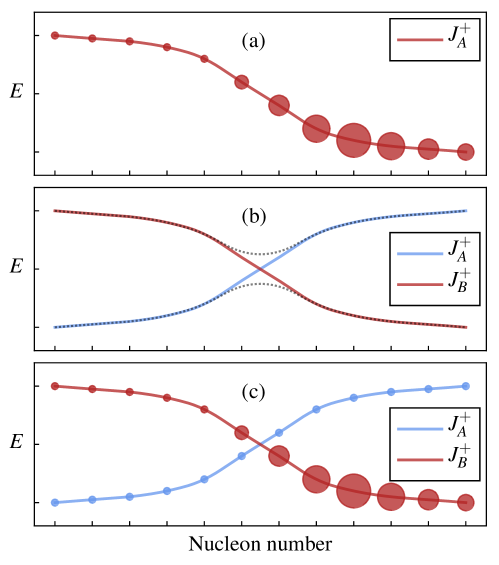
Figure 1: Schematic illustration for the evolution with nucleon number of energies (in arbitrary units) of the lowest $J^{+}$ states of one or two configurations, A and B. (a) Type I QPT: shape changes within a single configuration (small and large circles denote weak and strong deformation, respectively). (b) Type II QPT: coexisting and possibly crossing of two configurations, usually, with strong mixing. The dashed lines depict the mixing, as in a two states mixing scenario. (c) IQPTs: abrupt crossing of two configurations, with weak mixing, accompanied by a pronounced gradual shape evolution within each configuration.

The first QPT, Type I, is considered when nucleons are added in a single shell model configuration and a shape evolution occurs as one adds more nucleons, as shown schematically in Figure 1(a). The circles denote the amount of deformation and as more nucleons are added it increases, which lowers the absolute energy of the ground state. A Type I QPT can be described by the following Hamiltonian

$$\hat{H}=(1-\xi)\hat{H}_{1}+\xi\hat{H}_{2}~{}.$$ (1)

As the control parameter $\xi$ varies from 0 to 1, the equilibrium shape and symmetry of the Hamiltonian vary from those of $\hat{H}_{1}$ to those of $\hat{H}_{2}$.

The second QPT, Type II, is considered when nucleons are added in multiple shell model configurations that interact and cross. This is in the sense that higher lying states that are associated with nucleons residing in a higher configuration are lowered to become the ground state. This is shown schematically in Figure 1(b) where one observes what appears to resemble a two state mixing scenario. In this case, Type II QPTs can be described by a matrix Hamiltonian [8]

$$\hat{H}=\left[\begin{array}[]{cc}\hat{H}^{\rm A}(\xi^{\rm(A)})&\hat{W}(\omega)\\ \hat{W}(\omega)&\hat{H}^{\rm B}(\xi^{\rm(B)})\end{array}\right]$$ (2)

given here for two configurations, denoted by the indices $A$ and $B$, and $\hat{W}$ denotes their coupling.

Recently, studies have shown the occurrence of such crossing and shape evolution in the even-even zirconium (₄₀Zr) isotopes [9, 10, 11] and the adjacent odd-$A$ niobium (₄₁Nb) isotopes [12, 13]. This unique scenario has been termed as intertwined quantum phase transitions (IQPTs), which denotes the identification of both Types of QPTs, I and II, in the same chain of isotopes.

2 Theoretical framework

For the study of QPTs involving configuration crossing we shall use the algebraic framework of the interacting boson model with configuration mixing [14, 15, 16] for the even-even Zr isotopes and the interacting boson-fermion model with configuration mixing for the odd-mass Nb isotopes [12, 13].

2.1 IBM-CM

The IBM for a single shell model configuration has been widely used [14] to describe low-lying collective states in nuclei in terms of $N$ monopole ($s$) and quadrupole ($d$) bosons, representing valence nucleon pairs. The Hamiltonian interactions are Hermitian, rotationally invariant and conserve the total number of $s$ and $d$ bosons,

$$\hat{N}=\hat{n}_{s}+\hat{n}_{d}=s^{\dagger}s+\sum_{\mu}d^{\dagger}_{\mu}d_{\mu}~{}.$$ (3)

The number of bosons (3) is fixed by the microscopic interpretation of the IBM [17] to be the total number of proton and neutron particle or hole pairs counted from the nearest closed shell.

For excitations involving $n$-particles and $m$-holes ($n$p-$m$h) from multiple shell model configurations, one can extend the IBM to IBM with configuration mixing (IBM-CM) by associating each $n$p-$m$h excitations to a different $N$-boson space, such as 0p-0h ($N$), 2p-2h ($N+2$), 4p-4h ($N+4$), etc. In such a case, the Hamiltonian named $\hat{H}_{b}$ is written in matrix form, which for two configurations is written as in Eq. 2, where $\hat{H}_{b}^{\rm A}(\xi^{(\rm A)})$ represents the normal configuration ($N$ boson space, denoted henceforth by A) and $\hat{H}_{b}^{\rm B}(\xi^{(\rm B)})$ represents the intruder configuration ($N\!+\!2$ boson space, denoted henceforth by B), corresponding to 2p-2h excitations across the (sub-) shell closure (the subscript $b$ denotes that these are boson Hamiltonians). In this work, their form is

$$\hat{H}_{b}^{\rm A} =\epsilon^{\rm(A)}_{d}\hat{n}_{d}+\kappa^{\rm(A)}\hat{Q}_{\chi}\cdot\hat{Q}_{\chi}~{},$$ (4a)

$$\hat{H}_{b}^{\rm B} =\epsilon^{\rm(B)}_{d}\hat{n}_{d}+\kappa^{\rm(B)}\hat{Q}_{\chi}\cdot\hat{Q}_{\chi}+\kappa^{\rm\prime(B)}\hat{L}\cdot\hat{L}+\Delta~{},$$ (4b)

where $\Delta$ is the off-set energy between configurations A and B, the quadrupole operator is $\hat{Q}_{\chi}=d^{\dagger}s+s^{\dagger}\tilde{d}\!+\!\chi(d^{\dagger}\tilde{d})^{(2)}$, where $\tilde{d}_{\mu}\!=\!(-)^{\mu}d_{-\mu}$, and the mixing term is $\hat{W}_{\rm b}\!=\!\omega[(d^{\dagger}d^{\dagger})^{(0)}+(s^{\dagger})^{2}]+\rm{H.c.}$, where H.c. stands for Hermitian conjugate.

The Hamiltonian $\hat{H}_{b}^{i}$, with $i=\rm A,B$, can interpolate between three forms of dynamical symmetry (DS) limits using the control parameters $(\epsilon^{(i)}_{d},\kappa^{(i)},\chi)$ ($\kappa^{\prime(\rm B)}$ and $\Delta$ of $\hat{H}_{b}^{\rm B}$ do not affect the DS structure), where U(6) serves as its spectrum generating algebra and SO(3) its symmetry algebra

$$\rm{U(6)}\supset\left\{\begin{array}[]{cc}&\mkern-18.0mu\rm{U(5)}\supset\rm{SO(5)}\supset\rm{SO(3)}\\ &\mkern-72.0mu\rm{SU(3)}\supset\rm{SO(3)}\\ &\rm{SO(6)}\supset\rm{SO(5)}\supset\rm{SO(3)}\end{array}\right.$$ (4e)

In such a case, the spectrum is completely solvable and resembles known paradigms of collective motion: spherical vibrator [U(5)], axial deformed rotor [SU(3)] and $\gamma$-soft deformed rotor [SO(6)].

2.1.1 Boson $E2$ transitions operator.

For $E2$ transitions, the boson operator reads

$$\hat{T}_{b}(E2)=e^{(\rm A)}\hat{Q}^{(N)}_{\chi}+e^{(\rm B)}\hat{Q}^{(N+2)}_{\chi}~{},$$ (4f)

where $e^{(\rm A)},e^{(\rm B)}$ are the boson effective charges for configuration A and B, respectively, and superscript $(N)$ denotes a projection onto the $[N]$ boson space.

2.1.2 Boson wave functions.

The eigenstates $\ket{\Psi;L}$ of the boson Hamiltonian with angular momentum $L$, are linear combinations of the wave functions, $\Psi_{\rm A}$ and $\Psi_{\rm B}$, in the two spaces $[N]$ and $[N+2]$, $\ket{\Psi;L}=a\ket{\Psi_{\rm A};[N],L}+b\ket{\Psi_{\rm B};[N\!+\!2],L}$, with $a^{2}+b^{2}=1$. Each part of the wave functions with a given boson number $N$ and angular momentum $L$ can be expanded in terms of the DS bases of the IBM in the following manner

$$\ket{\Psi;[N],L} =\sum_{n_{d},\tau,n_{\Delta}}C^{(N,L)}_{n_{d},\tau,n_{\Delta}}\ket{N,n_{d},\tau,n_{\Delta},L} \qquad\left[\rm{U(5)}\right]$$ (4g)

$$=\sum_{(\lambda,\mu),K}C^{(N,L)}_{(\lambda,\mu),K}\ket{N,(\lambda,\mu),K,L} \qquad\left[\rm{SU(3)}\right]$$

$$=\sum_{\sigma,\tau,n_{\Delta}}C^{(N,L)}_{\sigma,\tau,n_{\Delta}}\ket{N,\sigma,\tau,n_{\Delta},L} \qquad\left[\rm{SO(6)}\right]$$

where $N,n_{d},(\lambda,\mu),\sigma,\tau,L$ label the irreducible representations of U(6), U(5), SU(3), SO(6), SO(5) and SO(3), respectively, and $n_{\Delta},K$ are multiplicity labels. The coefficients $C^{(N,L)}_{\alpha}$, with quantum numbers $\alpha$, give the weight of each component in the wave function. They can therefore give us the probability of having definite quantum numbers of a given symmetry. For example, for the U(6) DS the boson number $N$, which reveals the amount of normal-intruder mixing, and for the U(5) DS the $d$-boson number, $n_{d}$, which reveals the amount of deformation

$$P^{(N_{i},J)} =~{}~{}\sum_{n_{d}}P^{(N_{i},L)}_{n_{d}}~{};\quad i={\rm A,B}\quad\left(P^{(N_{\rm A},L)}+P^{(N_{\rm B},L)}=1\right)$$ (4ha)

$$P^{(N_{i},L)}_{n_{d}} =\sum_{\tau,n_{\Delta},L}|C^{(N_{i},L)}_{n_{d},\tau,n_{\Delta},L}|^{2}~{},$$ (4hb)

where $N_{\rm A}=N$ and $N_{\rm B}=N+2$.

2.2 IBFM-CM

The IBFM for a single shell model configuration has been widely used [18] to describe low-lying collective states of odd-mass nuclei, where a fermion is coupled to the boson Hamiltonian, which serves as a core. For two shell model configurations, 0p-0h and 2p-2h, the IBFM-CM framework [12, 13] Hamiltonian can be written in the following matrix form

$$\hat{H}=\hat{H}_{\rm b}+\hat{H}_{\rm f}+\hat{V}_{\rm bf}$$

$$\qquad=\left[\begin{array}[]{cc}\hat{H}_{b}^{\rm A}(\xi^{\rm(A)})&\hat{W}_{b}(\omega)\\ \hat{W}_{b}(\omega)&\hat{H}_{b}^{\rm B}(\xi^{\rm(B)})\end{array}\right]+\left[\begin{array}[]{cc}\sum_{j}\epsilon_{j}\hat{n}_{j}&0\\ 0&\sum_{j}\epsilon_{j}\hat{n}_{j}\end{array}\right]+\left[\begin{array}[]{cc}\hat{V}^{\rm A}_{bf}(\zeta^{(\rm A)})&\hat{W}_{bf}(\omega_{j})\\ \hat{W}_{bf}(\omega_{j})&\hat{V}^{\rm B}_{bf}(\zeta^{(\rm B)})j\end{array}\right]$$ (4ho)

The first part of $\hat{H}$ is the boson core with entries from Equations (4a)-(4b), the second part is the fermion Hamiltonian with single particle energies $\epsilon_{j}$ and the fermion number operator $\hat{n}_{j}$, the third part is the Bose-Fermi interaction. The latter has off diagonal parts that combine boson and fermion mixing terms and a diagonal part that typically takes the following form of monopole, quadrupole and exchange interactions $\hat{V}^{(i)}_{\rm bf}(A_{0},\Gamma_{0},\Lambda_{0})=V^{{\rm MON}(i)}_{\rm bf}(A_{0})+V^{{\rm QUAD}(i)}_{\rm bf}(\Gamma_{0})+V^{{\rm EXC}(i)}_{\rm bf}(\Lambda_{0})$, with $i=\rm A,B$ [18]. These Bose-Fermi interactions depend on the strengths $A_{0}$, $\Gamma_{0}$ and $\Lambda_{0}$, respectively, given from the microscopic theory of the IBFM (see [13] for more details).

2.2.1 Bose-Fermi $E2$ transitions

For $E2$ transitions, the boson-fermion operator reads

$$\hat{T}(E2)=\hat{T}_{b}(E2)+\hat{T}_{f}(E2)~{},$$ (4hp)

where the boson part, $\hat{T}_{b}(E2)$, is given in Equation (4f). The fermion part, $\hat{T}_{f}(E2)$, is given by

$$\hat{T}_{\rm f}(E2)=\sum_{jj^{\prime}}f^{(2)}_{jj^{\prime}}[a^{\dagger}_{j}\times\tilde{a}_{j^{\prime}}]^{(2)},$$ (4hq)

with $f^{(2)}_{jj^{\prime}}=-\frac{e_{f}}{\sqrt{5}}\braket{j}{Y^{(2)}_{lm}}{j^{\prime}}$, where $e_{f}$ is the effective charge for $E2$ transitions.

2.2.2 Bose-Fermi wave functions

The eigenstates of the Hamiltonian (2.2), $\ket{\Psi;J}$, are linear combinations of wave functions (4g), involving bosonic basis states in the two spaces $\ket{[N],\alpha,L}$ and $\ket{[N+2],\alpha,L}$, where $\alpha$ denotes additional quantum numbers characterizing the boson basis used. The boson ($L$) and fermion ($j$) angular momenta are coupled to a total $J$ and the combined wave function takes the form

$$\ket{\Psi;J}\!=\!\sum_{\alpha,L,j}C^{(N,J)}_{\alpha,L,j}\ket{\Psi_{\rm A};[N],\alpha,L,j;J}+\sum_{\alpha,L_{,}j}C^{(N+2,J)}_{\alpha,L,j}\ket{\Psi_{\rm B};[N+2],\alpha,L,j;J}~{},$$ (4hr)

For such a wave function, similarly as in Equations (4ha) and (4hb), it is possible to examine the probability of the quantum labels of the U(6) boson DS, $N$, and the U(5) boson DS, $n_{d}$,

$$P^{(N_{i},J)} =~{}~{}\sum_{n_{d}}P^{(N_{i},J)}_{n_{d}}~{},\quad i={\rm A,B}\quad\left(P^{(N_{\rm A},J)}+P^{(N_{\rm B},J)}=1\right)$$ (4hsa)

$$P^{(N_{i},J)}_{n_{d}} =\sum_{\tau,n_{\Delta},j,L}|C^{(N_{i},J)}_{n_{d},\tau,n_{\Delta},L,j}|^{2}~{}$$ (4hsb)

3 IQPTs in the zirconium and niobium chains

To describe the ₄₀Zr isotopes in the IBM-CM framework, we consider ${}_{40}^{90}$Zr as a core and valence neutrons in the 50–82 major shell. The normal A configuration corresponds to having no active protons above $Z\!=\!40$ sub-shell gap, and the intruder B configuration corresponds to two-proton excitation from below to above this gap, creating 2p-2h states (see [11] for more details). To describe the ₄₁Nb isotopes in the IBFM-CM framework we couple a proton to the respective ₄₀Zr cores with neutron number 52–62. In the present contribution, we focus on the positive-parity states in the Nb isotopes, which reduces to a single-$j$ calculation with the $1g_{9/2}$ orbit (a multi-$j$ calculation for negative-parity states can be found in [13]). The model space for ⁹⁹Nb is shown schematically in Figure 2, where ⁹⁸Zr serves as the boson core.

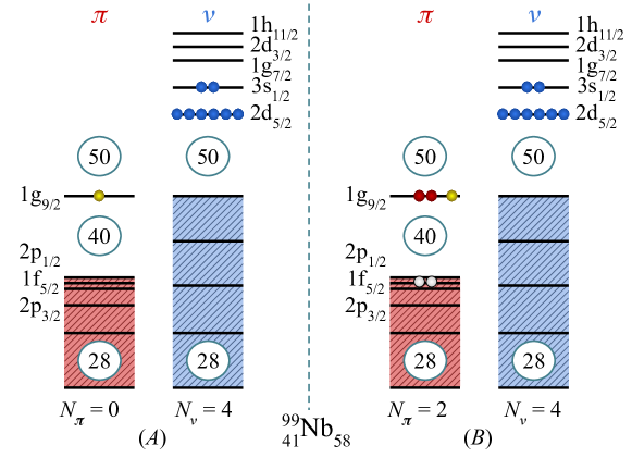
Figure 2: Schematic representation of the two coexisting shell-model configurations (A and B) for ${}^{99}_{41}$Nb₅₈, where ${}^{98}_{40}$Zr₅₈ serves as a core. The corresponding numbers of proton bosons ($N_{\pi}$) and neutron bosons ($N_{\nu}$), are listed for each configuration and $N=N_{\pi}+N_{\nu}$.

In order to understand the change in structure of the Zr and Nb isotopes, it is insightful to examine the evolution of observables along the chain. In this contribution, the observables include energy levels, two-neutron separation energies and $E2$ transition rates.

3.1 Evolution of energy levels

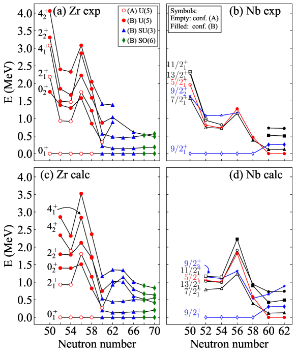
Figure 3: Panels (a) and (c): comparison between experimental and calculated energy levels of Zr isotopes. Panels (b) and (d): comparison between energy levels of Nb isotopes. Empty (filled) symbols indicate a states dominated by the normal A configuration (intruder B configuration), with assignments based on Equation (4ha) (Zr) and Equation (4hsa) (Nb). In panels (a) and (c), the shape of the symbols [$\circ,\triangle,\diamondsuit$], indicates the closest dynamical symmetry [U(5), SU(3), SO(6)] to the level considered, based on Equation (4hb). Note that the calculated values start at neutron number 52, while the experimental values include the closed shell at 50. References for the data are given at [11] (for Zr) and [13] (for Nb).

A comparison between experimental and calculated levels of Zr and Nb is shown in Figure 3, along with assignments to configurations based on Equation (4ha), for Zr, and Equation (4hsa), for Nb. For Zr, we also add symbols denoting the most dominant DS component in the wave function based on the decompositions of Equation (4hb), for each state (the definitions to the other SU(3) and SO(6) DS decompositions can be found in [11]).

For Zr isotopes, panels (a) and (c), in the region between neutron number 50 and 56, there appear to be two configurations, one spherical (seniority-like), A, and one weakly deformed, B, as evidenced by the ratio $R_{4/2}$, which is at 52–56, $R^{\rm(A)}_{4/2}\cong 1.6$ and $R^{\rm(B)}_{4/2}\cong 2.3$. Their trend decreases at neutron number 52–54, away from the closed shell, and rise again at 56 due to the $\nu(2d_{5/2})$ subshell closure. From neutron number 58, there is a pronounced drop in energy for the states of configuration B and at 60, the two configurations exchange their role indicating a Type II QPT. At this stage, the intruder B configuration appears to be at the critical point of a U(5)-SU(3) Type I QPT, as evidenced by the low value of the excitation energy of the first excited $0^{+}$ state of this configuration (the $0^{+}_{3}$ state in ¹⁰⁰Zr shown in Figure 3 of [9]). Beyond neutron number 60, the intruder configuration (B) is strongly deformed, as evidenced by the small value of the excitation energy of the state $2_{1}^{+}$, $E_{2_{1}^{+}}\!=\!139.3$ keV and by the ratio $R^{\rm(B)}_{4/2}\!=\!3.24$ in ¹⁰⁴Zr. At still larger neutron number 66, the ground state band becomes $\gamma$-unstable (or triaxial) as evidenced by the close experimental energy of the states $2_{2}^{+}$ and $4_{1}^{+}$, $E_{2_{2}^{+}}\!=\!607.0$ keV, $E_{4_{1}^{+}}\!=\!476.5$ keV, in ¹⁰⁶Zr, and especially by the experimental $E_{4^{+}_{1}}\!=\!565$ keV and $E_{2^{+}_{2}}\!=\!485$ keV in ¹¹⁰Zr, a signature of the SO(6) symmetry. In this region, the ground state configuration undergoes a crossover from SU(3) to SO(6).

For Nb isotopes, panels (b) and (d), we see a quintuplet of states ($5/2^{+}_{1},7/2^{+}_{1},11/2^{+}_{2},13/2^{+}_{1},9/2^{+}_{2}$). For neutron number 52–56, their energy varies due to the filling of the $\nu(2d_{5/2})$ shell. At neutron number 58, there is a pronounced drop in energy for the states of the B configuration, due to the onset of deformation. At 60, the two configurations cross, indicating a Type II QPT, and the ground state changes from $9/2^{+}_{1}$ to $5/2^{+}_{1}$, becoming the bandhead of a $K=5/2^{+}$ rotational band composed of $5/2^{+}_{1},7/2^{+}_{1},9/2^{+}_{1},11/2^{+}_{1},13/2^{+}_{1},\ldots$ states. At this point the intruder B configuration also undergoes a Type I QPT from a weak to a strong coupling scenario. Beyond neutron number 60, the intruder B configuration remains strongly deformed and the band structure persists. The above trend is similar to that encountered in the even-even ₄₀Zr cores.

The comparability to the even-even Zr cores comes from the fact that four of the states in Figure 3, ($5/2^{+}_{1},7/2^{+}_{1},11/2^{+}_{2},13/2^{+}_{1}$), have the same trend as the $2^{+}_{1}$ state of the adjacent Zr isotopes and one state, ($9/2^{+}_{2}$), like the $0^{+}_{2}$. For 52–58, the correspondence occurs since the Zr $L=2^{+}_{1}$ state is coupled to single $j=9/2$ orbit through a weak coupling scenario giving a total angular momentum of $|L-j|\leq J\leq|L+j|$ (note that the $J=9/2^{+}$ which is part of this quintuplet is the $9/2^{+}_{3}$ and is not shown in the figure). In such a scenario, the “center of gravity” [19] of the Nb multiplet is centered around the energy of the $2^{+}_{1}$, as described in [13]. The same occurs for the $9/2^{+}_{2}$ of Nb and the $0^{+}_{2}$ of Zr.

3.2 Evolution of configuration and symmetry content

\begin{overpic}[width=303.53267pt]{fig_Nb_Zr_SDANCA23_nd_decomp_3.pdf} \put(10.0,25.0){\scriptsize\fcolorbox{black}{white}{(a) Intruder component}} \put(48.7,46.0){\scriptsize\fcolorbox{black}{white}{(b) $n_d=0$ component}} \end{overpic}

Figure 4: Percentage of (a) the intruder B component, Equations (4ha) and (4hsa), (b) the boson U(5) $n_{d}=0$ component, Equations (4hb) and (4hsb), of ^52-110Zr (red lines) and ^93-103Nb (blue lines) isotopes, respectively. On top of panel (b) shown are the boson DS indicating the transitions in symmetry within the intruder B configuration. For Nb isotopes, the ground state $J^{+}_{gs}$ ($J^{+}_{B}$) is $9/2^{+}_{1}$ ($9/2^{+}_{2}$) for ^93-99Nb and $5/2^{+}_{1}$ ($5/2^{+}_{2}$) for ^101,103 Nb and

To understand the occurrence of both Type II and I QPTs in the chain of Zr and Nb isotopes, we examine explicitly the evolution of the intruder and of the U(5) symmetry components of the wave function.

For the Type II QPT, we examine in Figure 4(a) the intruder component of the wave function of the ground state of Zr ($P^{(N_{\rm B},0^{+}_{gs})}$) and Nb ($P^{(N_{\rm B},J^{+}_{gs})}$) isotopes, Equations (4ha) and (4hsa), respectively. We observe the same trend, where from neutron number 52 to 58 this component is small and at 60 it jumps to about 87% in Zr and 99% in Nb and remains at about 99% for the heavier isotopes in both chains. This is the occurrence of the Type II QPT, where the ground state changes its configuration content from normal (at neutron number 58) to intruder (at 60).

For the Type I QPT within configuration B, we examine in Figure 4(b) the $n_{d}=0$ component of the configuration B part of $0^{+}_{B}=0^{+}_{2}$ for ^92-98Zr and $0^{+}_{B}=0^{+}_{1}$ for ^100-110Zr ($P^{(N_{\rm B},0^{+}_{B})}_{n_{d}=0}$) and of $J^{+}_{B}=9/2^{+}_{2}$ for ^93-99Nb and $J^{+}_{B}=5/2^{+}_{1}$ for ^101-103Nb ($P^{(N_{\rm B},J^{+}_{B})}_{n_{d}=0}$). The circles represent the percentage of the U(5) $n_{d}\!=\!0$ component in the wave function, Equations (4hb) and (4hsb). For Zr, it is large ($\approx 90\%$) for neutron number 52–58 and drops drastically ($\approx 30\%$) at 60. The drop means that other $n_{d}\!\not=\!0$ components are present in the wave function and therefore this state becomes deformed. Above neutron number 60, the $n_{d}\!=\!0$ component drops almost to zero (and rises again a little at 70), indicating the state is strongly deformed. For Nb we see the exact same trend, however, the total value of $P^{(N_{\rm B},J^{+}_{B})}_{n_{d}=0}$ is smaller, indicating that for odd-mass nuclei coupling the fermion to the boson core increases deformation.

3.3 Evolution of two neutron separation energies

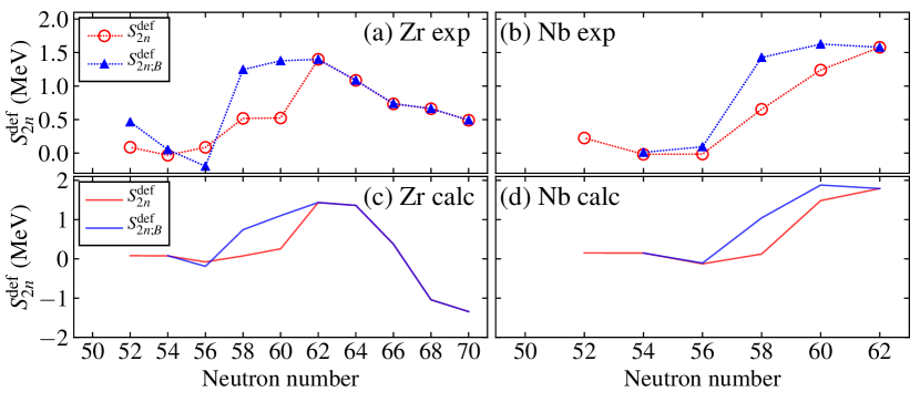
Figure 5: Comparison of the deformed part of the two neutron separation energies, ($S^{\rm def}_{2n}$), between Zr and Nb experiment (a) and (b) [20] and Zr and Nb calculation (c) and (d), respectively.

An observable that portrays both types of QPTs is two neutron separation energy, defined as

$$S_{2n}=2M_{n}+M(N-2,Z)-M(N,Z),$$ (4hst)

where $M(N,Z)$ is the mass of a nuclei with $N,Z$ neutrons and protons, respectively, and $M_{n}$ is the neutron mass. In the IBM and IBFM, it is convenient to transcribe the $S_{2n}$ as

$$S_{2n}=-\tilde{A}-\tilde{B}N_{v}\pm S^{\rm def}_{2n}-\Delta_{n},$$ (4hsu)

where $N_{v}$ is half the number of valence particles in the boson core and $S^{\rm def}_{2n}$ is the contribution of the deformation, obtained by the expectation value of the Hamiltonian in the ground state. The $+$ sign applies to particles and the $-$ sign to holes. The $\Delta_{n}$ parameter takes into account the neutron subshell closure at 56, $\Delta_{n}=0$ for 50–56, and $\Delta_{n}=2$ MeV for 58–70 for Zr (58–62 for Nb). Its value is adapted from [21]. For the Zr (Nb) isotopes, the chosen values in Eq. 4hsu are $\tilde{A}=-17.25$ ($-16.5$) and $\tilde{B}=0.758$ MeV. The value of $\tilde{A}$ is taken to fit ⁹⁰Zr (⁹¹Nb), and the value of $\tilde{B}$ is taken from a fit to the binding energies of ^92,94,96Zr. In Figure 5, the Zr and Nb experimental and calculated deformed part, $S^{\rm def}_{2n}$ [22, 23], are shown in red open circles and lines, respectively. $S^{\rm def}_{2n}$ is obtained by subtracting the linear part and $\Delta_{n}$ from the experimental and calculated $S_{2n}$. One can clearly see the onset of deformation going from neutron number 52–56, where $S^{\rm def}_{2n}$ is close to zero, to 58–62, where it jumps and rises in both Zr and Nb isotopes. For Zr, we also see after neutron number 62 a gradual decrease in $S^{\rm def}_{2n}$ due to the crossover towards SO(6) symmetry.

In order to denote the occurrence of both Type I and II QPTs, in addition to Equation (4hsu), it is also possible using Equation (4hst) to estimate two neutron separation energies for excited states, by using the mass of an excited state $M(N,Z)\!\equiv\!M_{exc}(N,Z)=M_{gs}(N,Z)+E_{exc}(N,Z)$, where $M_{gs}(N,Z)$ is the mass for the ground state and $E_{exc}(N,Z)$ is the energy of the excited state [13]. We choose the lowest configuration B state for this case in both Zr and Nb isotopes. The experimental and calculated results, $S^{\rm def}_{2n;B}$, are given in blue triangles and lines, in Figure 5. For both Zr and Nb isotopes, it is seen that for neutron number 54–56 $S^{\rm def}_{2n;B}$ is close to zero, then at 58 it jumps due to the onset of deformation, then it flattens at 60. This behavior denotes the Type I QPT of shape evolution within configuration B of Zr (Nb) from spherical (weak coupling) to axially-deformed (strong coupling). For neutron number 54–56, $S^{\rm def}_{2n;B}$ (triangles) is close to the value of $S^{\rm def}_{2n}$ (circles), as configuration B is more spherical. At 58, there is a larger jump than $S^{\rm def}_{2n}$ since configuration B is more deformed than A, which continues at 60. For 62 (and 64–70 for Zr), both $S^{\rm def}_{2n;B}$ and $S^{\rm def}_{2n}$ coincide since the ground state is configuration B, which denotes the Type II QPT.

3.4 Evolution of $E2$ transition rates

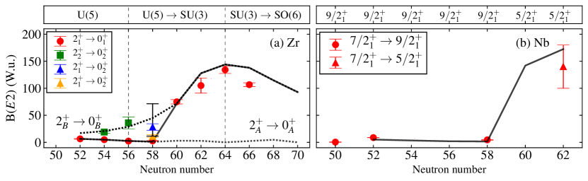
Figure 6: $B(E2)$ values in W.u. (a) for $2^{+}\to 0^{+}$ transitions in the Zr chain and (b) for $7/2^{+}_{1}\to J^{+}_{gs}$ in the Nb chain, where $J^{+}_{gs}$ is given in the panel above (b). On top of panel (a) shown are the boson dynamical symmetries indicating the transitions in symmetry within the intruder B configuration. The solid line (symbols ${\color[rgb]{1,0,0}\CIRCLE},~{}{\color[rgb]{0,0.5,0}\blacksquare},~{}{\color[rgb]{0,0,1}\blacktriangle},~{}{\color[rgb]{1,.5,0}\blacklozenge}$) denote calculated results (experimental results). In (a), dotted lines denote calculated $E2$ transitions within a configuration. References for the data can be found in [11].

The occurrence of both Type I and II QPTs are also stressed by an analysis of $B(E2)$ values. As shown in Fig. 6(a) for Zr, the calculated $2^{+}_{A}\to 0^{+}_{A}$ transition rates coincide with the empirical $2^{+}_{1}\to 0^{+}_{1}$ rates for neutron numbers 52–56. The calculated $2^{+}_{B}\to 0^{+}_{B}$ transition rates coincide with the empirical $2^{+}_{2}\to 0^{+}_{2}$ rates for neutron numbers 52–56, with the empirical $2^{+}_{1}\to 0^{+}_{2}$ rates at 58 and with the empirical $2^{+}_{1}\to 0^{+}_{1}$ rates at 60–64. The large jump in $B(E2;2^{+}_{1}\!\to\!0^{+}_{1})$ between 58 and 60 reflects the passing through a critical point, common to a Type II QPT involving a crossing of two configurations. The further increase in $B(E2;2^{+}_{1}\!\to\!0^{+}_{1})$ for neutron numbers 60–64 is as expected from a U(5)-SU(3) Type I QPT and reflects an increase in the deformation in a spherical to deformed shape-phase transition within configuration B. The subsequent decrease from the peak at neutron number 64 towards 70 is expected from an SU(3) to SO(6) crossover. The same trend at neutron number 52–62 in the $B(E2)$ value Zr can be observed in Fig. 6(b) for the Nb isotopes. Although there is less data, the $B(E2)$ values from the first excited to the ground state are small for neutron number 52–58 and at 60 there is large jump, which continues to increase towards 62, possibly suggesting even stronger deformation than in the adjacent Zr, although the experimental error bar is large.

4 Conclusions and outlook

The general framework of the interacting boson model and interacting boson-fermion model with configuration mixing, IBM-CM and IBFM-CM, respectively, has been presented, allowing a quantitative description of shape-coexistence (configuration-mixing) and related QPTs in even-even and odd-mass nuclei. By employing such a comparison, odd-mass nuclei can serve as a further test case for shape coexistence in even-even nuclei by verifying whether the even-even core is the right one to describe the adjacent odd-mass nucleus.

A quantal analysis for the chain of the even-even ₄₀Zr and odd-mass ₄₁Nb isotopes involving positive-parity states was performed for neutron number 52–70 (Zr) and 52–62 (Nb). It examined the evolution of energy levels, two-neutron separation energies and $E2$ transition rates along both chains. Special attention has been devoted to changes in the configuration-content and U(5) content of wave functions.

The results of the analysis suggest a complex phase structure yet similar in both chains of these isotopes, involving two configurations. The two configurations cross near neutron number 60, and the ground state changes from configuration A to configuration B, demonstrating a Type II QPT. They are weakly mixed and retain their purity before and after the crossing. Alongside the Type II QPT, the intruder B configuration undergoes a spherical-U(5) (weak coupling) to axially-deformed-SU(3) (strong coupling) QPT within the boson core (Bose-Fermi Hamiltonian), with a critical point near $A\approx 100$, thus demonstrating, IQPTs in both even-even and odd-mass nuclei.

References

References

- [1] Heyde K and Wood J L 2011 Rev. Mod. Phys. 83 1467–1521
- [2] Garrett P E, Zielińska M and Clément E 2022 Prog. Part. Nucl. Phys. 124 103931
- [3] Federman P and Pittel S 1979 Phys. Rev. C 20 820–829
- [4] Togashi T, Tsunoda Y, Otsuka T and Shimizu N 2016 Phys. Rev. Lett. 117 172502
- [5] Cejnar P, Jolie J and Casten R F 2010 Rev. Mod. Phys. 82 2155–2212
- [6] Gilmore R and Feng D H 1978 Nucl. Phys. A 301 189–204
- [7] Gilmore R 1979 J. Math. Phys. 20 891–893
- [8] Frank A, Van Isacker P and Iachello F 2006 Phys. Rev. C 73 061302(R)
- [9] Gavrielov N, Leviatan A and Iachello F 2019 Phys. Rev. C 99 064324
- [10] Gavrielov N, Leviatan A and Iachello F 2020 Phys. Scr. 95 024001
- [11] Gavrielov N, Leviatan A and Iachello F 2022 Phys. Rev. C 105 014305
- [12] Gavrielov N, Leviatan A and Iachello F 2022 Phys. Rev. C 106 L051304
- [13] Gavrielov N 2023 Phys. Rev. C 108 014320
- [14] Iachello F and Arima A 1987 The Interacting Boson Model (Cambridge University Press)
- [15] Duval P D and Barrett B R 1981 Phys. Lett. B 100 223–227
- [16] Duval P D and Barrett B R 1982 Nucl. Phys. A 376 213–228
- [17] Iachello F and Talmi I 1987 Rev. Mod. Phys. 59 339–361
- [18] Iachello F and Van Isacker P 1991 The Interacting Boson-Fermion Model (Cambridge University Press)
- [19] Lawson R D and Uretsky J L 1957 Phys. Rev. 108 1300–1304
- [20] Wang M, Huang W, Kondev F, Audi G and Naimi S 2021 Chinese Phys. C 45 030003
- [21] Barea J and Iachello F 2009 Phys. Rev. C 79 044301
- [22] Petrellis D, Leviatan A and Iachello F 2011 Ann. Phys. 326 926–957
- [23] Iachello F, Leviatan A and Petrellis D 2011 Phys. Lett. B 705 379–382