C-RAG: Certified Generation Risks for Retrieval-Augmented Language Models

Mintong Kang
UIUC
mintong2@illinois.edu
&Nezihe Merve Gürel
TU Delft
n.m.gurel@tudelft.nl
&Ning Yu
Salesforce Research
ning.yu@salesforce.com
&Dawn Song
UC Berkeley
dawnsong@berkeley.edu
&Bo Li
UChicago & UIUC
bol@uchicago.edu
Abstract

Despite the impressive capabilities of large language models (LLMs) across diverse applications, they still suffer from trustworthiness issues, such as hallucinations and misalignments. Retrieval-augmented language models (RAG) have been proposed to enhance the credibility of generations by grounding external knowledge, but the theoretical understandings of their generation risks remains unexplored. In this paper, we answer: 1) whether RAG can indeed lead to low generation risks, 2) how to provide provable guarantees on the generation risks of RAG and vanilla LLMs, and 3) what sufficient conditions enable RAG models to reduce generation risks. We propose C-RAG, the first framework to certify generation risks for RAG models. Specifically, we provide conformal risk analysis for RAG models and certify an upper confidence bound of generation risks, which we refer to as conformal generation risk. We also provide theoretical guarantees on conformal generation risks for general bounded risk functions under test distribution shifts. We prove that RAG achieves a lower conformal generation risk than that of a single LLM when the quality of the retrieval model and transformer is non-trivial. Our intensive empirical results demonstrate the soundness and tightness of our conformal generation risk guarantees across four widely-used NLP datasets on four state-of-the-art retrieval models.

1 Introduction

Large language models (LLMs) (Touvron et al., 2023; OpenAI et al., 2023) recently exhibit emergent abilities across different NLP tasks, such as text summarization, question answering, and machine translation. However, existing works (Wang et al., 2023a; Liang et al., 2022; Liu et al., 2023) show that the generations of LLMs can be unreliable, untrustworthy, and risky in many cases. Therefore, certifiably controlling the generation risks of LLMs becomes particularly important before the deployment of LLMs, especially in safety-critical domains.

Retrieval-augmented language models (RAG) (Lewis et al., 2020; Karpukhin et al., 2020; Xiong et al., 2020) have been proposed to enhance the credibility of LLMs by retrieving relevant documents from an external knowledge base and generating contents conditioned on the retrieved knowledge. RAG models are shown effective in mitigating generation risks via in-context learning from the retrieved documents (Brown et al., 2020). However, theoretical understandings of their generation risks still remain unexplored. In this work, we focus on this problem and ask:

Can RAG indeed lead to low generation risks? How can we provide provable guarantees on the generation risks of RAG and vanilla LLMs? What are the sufficient conditions that enable RAG models to reduce generation risks? Can we provably control the generation risks below a desired level?

To theoretically analyze the generation risks of RAG and answer the above questions, we propose C-RAG, the first framework of certified generation risks for RAG models. We first propose a constrained generation protocol for RAG models to produce a controlled set of generations. The protocol operates based on specific parameter configurations, including the number of retrieved examples, the size of the generation set, and a similarity threshold for generation diversity. We then provide conformal analysis (Bates et al., 2021; Angelopoulos et al., 2021, 2022) for RAG models under the constrained generation protocol, aiming to provably control the generation risks based on test statistics from in-distribution calibration samples. To achieve this goal, we derive a high-probability upper bound of generation risks during inference time, which we call conformal generation risk. We show that (a) the conformal generation risk serves as a sound upper bound to the empirical generation risks given a RAG configuration in Proposition 1; (b) the generation risk can be certifiably controlled below a desired level by computing a valid set of RAG configurations via C-RAG in Proposition 2; (c) the conformal analysis can be extended to more complex scenarios under test-time distribution shifts in Theorem 2, which presents the first generation risk guarantee under test-time distribution shifts for general bounded risk functions. Based on our conformal analysis for the generation risks of RAG and vanilla LLMs, we prove that (a) the conformal generation risk of RAG is lower than that of the corresponding vanilla LLM in Theorem 1; (b) under bounded test-time distribution shifts, RAG also lowers the conformal generation risks compared to the vanilla LLM in Theorem 3.

We evaluate the conformal generation risk guarantees of C-RAG with different retrieval models on four widely-used datasets. For all retrieval methods and datasets, we empirically validate that our conformal generation risk guarantees are sound and tight even with distribution shifts, as they upper bound the empirical generation risks observed on random test sets while maintaining only a minimal gap, narrowing down to the scale of 1e31𝑒31e-3. We empirically show that RAG consistently achieves a lower conformal generation risk than a single LLM without retrieval, which is consistent with our theoretical findings in Sections 4 and 5. We also evaluate the conformal generation risk for different SOTA retrieval models, such as sparse encoding metrics BM25 (Robertson et al., 2009), text-embedding-ada-002 model from OpenAI, bge model from BAAI (Zhang et al., 2023a), and supervised fine-tuned embedding model (Wang et al., 2023b) to validate our analysis on retrieval quality. We show that among these models, text-embedding-ada-002 and supervised fine-tuned embedding models outperform other baselines in achieving low conformal generation risks.

2 Related work

Retrieval augmented generation (RAG) is a framework for improving the generation quality of LLMs via retrieving relevant information from an external knowledge base and grounding the model on the retrieved knowledge for conditional generations. SOTA retrieval methods (Lewis et al., 2020; Karpukhin et al., 2020; Xiong et al., 2020) employ dual encoders to project both query and candidate texts into the embedding space and retrieve candidate texts that exhibit high similarity to the embedded query text. Although RAG is demonstrated to be effective in enhancing the generation credibility, their theoretical understanding is limited. Basu et al. conduct retrieval analysis for a constrained function and data class from a statistical perspective, but the results cannot be applicable to self-attention transformers and to arbitrary data distribution. In this work, we provide the first theoretical analysis of how RAG leads to low generation risks in self-attention transformers for arbitrary data distribution.

Conformal prediction is a statistical technique used to create prediction sets with assured coverage. (Vovk et al., 1999, 2005; Lei et al., 2013; Yang & Kuchibhotla, 2021). Broadly, conformal risk control methods (Bates et al., 2021; Angelopoulos et al., 2021, 2022; Quach et al., 2023) provide a high-confidence risk guarantee for black-box risk functions, assuming data exchangeability. However, the risk guarantee can be broken under test-time distribution shifts. While Angelopoulos et al. and Farinhas et al. offer a valid conformal risk guarantee for monotonic risk functions under distribution shifts, the monotonicity assumption is not always practical. In this work, we introduce the first conformal risk guarantee for general bounded risk functions, under distribution shifts at test time.
Refer to caption
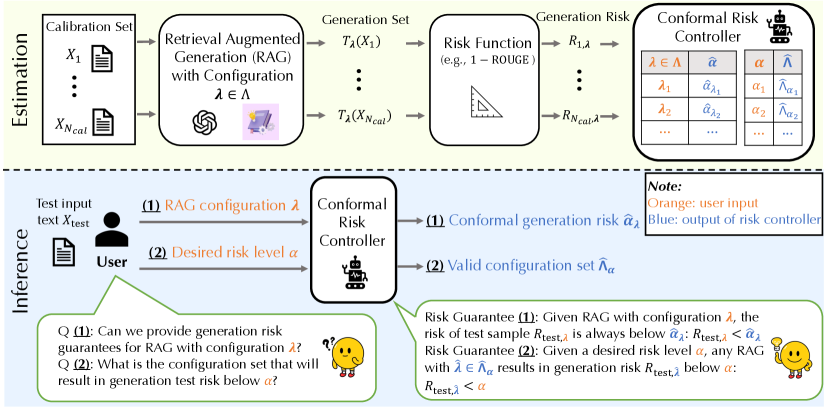
Figure 1: Overview of C-RAG. In the estimation stage (upper row), the conformal risk controller computes conformal generation risks for different RAG configurations (Proposition 1), and valid configuration sets for different risk levels (Proposition 2), both based on risk statistics on the calibration set. In the inference stage (lower row), for any configuration 𝝀𝝀{\bm{\lambda}} and any desired risk level α𝛼\alpha provided by users, the conformal risk controller outputs the conformal generation risk α^𝝀subscript^𝛼𝝀\hat{\alpha}_{\bm{\lambda}} with Risk Guarantee (1) and the configuration set Λ^αsubscript^Λ𝛼\hat{\Lambda}_{\alpha} with Risk Guarantee (2).

3 Conformal generation risks of RAG models

We introduce the problem setup in Section 3.1, our constrained generation protocol for RAG models in Section 3.2, and the conformal generation risks in Section 3.3. We prove that (1) Given a RAG configuration, C-RAG provides a high-probability generation risk upper bound in Proposition 1, and (2) Given a desired risk level α𝛼\alpha, C-RAG offers a set of configurations that can provably maintain the risk below α𝛼\alpha in Proposition 2.

3.1 Problem setup

For a pretrained language model (LM) and any user input text, we aim to provide rigorous guarantees for the generation risks (e.g., 1ROUGE1ROUGE1-\text{ROUGE}). To achieve this, we develop a constrained generation protocol for RAG models. The generation protocol is governed by adjustable parameter configurations (e.g., number of retrieved examples, size of generations), which allow for more controlled RAG generations to achieve a desired risk level.

Formally, we let 𝒱𝒱{\mathcal{V}} be the vocabulary set, nIsubscript𝑛𝐼n_{I} be the maximal length of input text and nOsubscript𝑛𝑂n_{O} be the maximal length of output text. Let 𝒳:=𝒱nIassign𝒳superscript𝒱subscript𝑛𝐼{\mathcal{X}}:={\mathcal{V}}^{n_{I}} be the input text space, and 𝒴:=𝒱nOassign𝒴superscript𝒱subscript𝑛𝑂{\mathcal{Y}}:={\mathcal{V}}^{n_{O}} be the output text space. We notate pθl(y|x)(x𝒳,y𝒴)subscript𝑝subscript𝜃𝑙conditional𝑦𝑥formulae-sequence𝑥𝒳𝑦𝒴p_{\theta_{l}}(y|x)~{}(x\in{\mathcal{X}},y\in{\mathcal{Y}}) as the probability distribution of output text y𝑦y given input text x𝑥x, estimated by a pretrained LM parameterized by θlsubscript𝜃𝑙\theta_{l}. Consider a RAG generation protocol T𝝀,pθl:𝒳2𝒴:subscript𝑇𝝀subscript𝑝subscript𝜃𝑙maps-to𝒳superscript2𝒴T_{{\bm{\lambda}},p_{\theta_{l}}}:{\mathcal{X}}\mapsto 2^{\mathcal{Y}} with LM θlsubscript𝜃𝑙\theta_{l} and parameter configuration 𝝀Λ=B𝝀Λsuperscript𝐵{\bm{\lambda}}\in\Lambda={\mathbb{R}}^{B}, where B𝐵B is the maximal number of parameters to control the generation procedure. To evaluate the quality of the generation under T𝝀,pθl(x)subscript𝑇𝝀subscript𝑝subscript𝜃𝑙𝑥T_{{\bm{\lambda}},p_{\theta_{l}}}(x) given input x𝑥x, we define a risk function R(T𝝀,pθl(x),y):2𝒴×𝒴[0,1]:𝑅subscript𝑇𝝀subscript𝑝subscript𝜃𝑙𝑥𝑦maps-tosuperscript2𝒴𝒴01R(T_{{\bm{\lambda}},p_{\theta_{l}}}(x),y):2^{\mathcal{Y}}\times{\mathcal{Y}}\mapsto[0,1], where y𝑦y is the reference text of x𝑥x. For text generation tasks, a typical selection of the risk function could be 1maxyT𝝀,pθl(x)ROUGE(y,y)1subscriptsuperscript𝑦subscript𝑇𝝀subscript𝑝subscript𝜃𝑙𝑥ROUGEsuperscript𝑦𝑦1-\max_{y^{\prime}\in T_{{\bm{\lambda}},p_{\theta_{l}}}(x)}\text{ROUGE}(y^{\prime},y), where ROUGE measures the matching score between the generation ysuperscript𝑦y^{\prime} and reference text y𝑦y. Notably, our generation protocol outputs a set of generations instead of just one, allowing us to explore better generations and adjust the generation set size through a parameter for risk control.

3.2 Constrained generation protocol for RAG models

RAG models (Wang et al., 2023b; Rubin et al., 2021; Huang et al., 2023) combine a retrieval model and a generation LM. The retrieval model retrieves Nragsubscript𝑁ragN_{\text{rag}} relevant examples to the query from an external knowledge base, and the LM learns in-context from these examples. The knowledge base contains Nextsubscript𝑁extN_{\text{ext}} samples in 𝒟^ext={(Xi,Yi)}i=1Nextsubscript^𝒟extsuperscriptsubscriptsubscript𝑋𝑖subscript𝑌𝑖𝑖1subscript𝑁ext\hat{{\mathcal{D}}}_{\text{ext}}=\{(X_{i},Y_{i})\}_{i=1}^{N_{\text{ext}}}. The retrieval model uses an encoder to map instances into an embedding space, and then identifies the relevant examples to the query Xtestsubscript𝑋testX_{\text{test}} based on similarity. This similarity, defined by sθr(,):𝒳×𝒳:subscript𝑠subscript𝜃𝑟maps-to𝒳𝒳s_{\theta_{r}}(\cdot,\cdot):{\mathcal{X}}\times{\mathcal{X}}\mapsto{\mathbb{R}} and parameterized by θrsubscript𝜃𝑟\theta_{r}, is used to find the nearest examples using KNN search in the embedding space.

We arrange the retrieved Nragsubscript𝑁ragN_{\text{rag}} in-context examples and the test example Xtestsubscript𝑋testX_{\text{test}} into augmented input text X(rag)superscript𝑋(rag)X^{\text{(rag)}} using a template. We then sample the generation from pθl(|X(rag))p_{\theta_{l}}(\cdot|X^{\text{(rag)}}) repeatedly until λgsubscript𝜆𝑔\lambda_{g} generations are collected. To control the diversity of generations, we reject those with a similarity higher than a threshold λssubscript𝜆𝑠\lambda_{s} to the previous generations. In essence, the constrained generation protocol is controlled by configuration 𝝀=[Nrag,λg,λs]𝝀subscript𝑁ragsubscript𝜆𝑔subscript𝜆𝑠{\bm{\lambda}}=[N_{\text{rag}},\lambda_{g},\lambda_{s}] and output a generation set T𝝀,pθl(x)subscript𝑇𝝀subscript𝑝subscript𝜃𝑙𝑥T_{{\bm{\lambda}},p_{\theta_{l}}}(x) based on the configuration 𝝀𝝀{\bm{\lambda}} and input x𝑥x. We refer to Algorithm 1 in Section C.1 for the pseudocode of the protocol.

3.3 Conformal generation risks for RAG models

We certify generation risks of the RAG models with the constrained generation protocol T𝝀,pθlsubscript𝑇𝝀subscript𝑝subscript𝜃𝑙\normalsize T_{{\bm{\lambda}},p_{\theta_{l}}} via conformal risk analysis (Bates et al., 2021; Angelopoulos et al., 2022, 2021). Conformal analysis provably controls the generation risks based on test statistics from in-distribution calibration samples. In this work, we consider a calibration set 𝒟^cal={(Xi,Yi)}i=1Ncalsubscript^𝒟calsuperscriptsubscriptsubscript𝑋𝑖subscript𝑌𝑖𝑖1subscript𝑁cal\hat{{\mathcal{D}}}_{\text{cal}}=\{(X_{i},Y_{i})\}_{i=1}^{N_{\text{cal}}} with size Ncalsubscript𝑁cal\normalsize N_{\text{cal}}, and compute the empirical generation risk R^(𝒟^cal)=1/Ncal(x,y)𝒟^calR(T𝝀,pθl(x),y)^𝑅subscript^𝒟cal1subscript𝑁calsubscript𝑥𝑦subscript^𝒟cal𝑅subscript𝑇𝝀subscript𝑝subscript𝜃𝑙𝑥𝑦\hat{R}(\hat{{\mathcal{D}}}_{\text{cal}})=\nicefrac{{1}}{{N_{\text{cal}}}}\sum_{(x,y)\in\hat{{\mathcal{D}}}_{\text{cal}}}R(T_{{\bm{\lambda}},p_{\theta_{l}}}(x),y).

Risk Guarantees for RAG Models

For an LM θlsubscript𝜃𝑙\theta_{l}, calibration set 𝒟^calsubscript^𝒟cal\hat{{\mathcal{D}}}_{\text{cal}}, test sample (Xtest,Ytest)subscript𝑋testsubscript𝑌test(X_{\text{test}},Y_{\text{test}}), generation protocol T𝝀,pθlsubscript𝑇𝝀subscript𝑝subscript𝜃𝑙T_{{\bm{\lambda}},p_{\theta_{l}}} with configuration 𝝀𝝀{\bm{\lambda}} and confidence level 1δ(δ[0,1])1𝛿𝛿011-\delta~{}(\delta\in[0,1]), C-RAG provides two types of generation risk guarantees for RAG models:

Proposition 1 (Risk Guarantee (1)).

Given a configuration 𝛌𝛌{\bm{\lambda}} in generation protocol, C-RAG guarantees that:

[R(T𝝀,pθl(x),y)α^𝝀]1δ,delimited-[]𝑅subscript𝑇𝝀subscript𝑝subscript𝜃𝑙𝑥𝑦subscript^𝛼𝝀1𝛿\normalsize{\mathbb{P}}\left[R(T_{{{\bm{\lambda}}},p_{\theta_{l}}}(x),y)\leq\hat{\alpha}_{\bm{\lambda}}\right]\geq 1-\delta,\vspace{\pspace} (1)

where the high-probability risk upper bound α^𝛌subscript^𝛼𝛌\hat{\alpha}_{\bm{\lambda}}, the so-called conformal generation risk, is given by:

α^=min{h1(1/δNcal;R^(𝒟^cal)),Φbin1(δe;Ncal,R^(𝒟^cal))}^𝛼superscript11𝛿subscript𝑁cal^𝑅subscript^𝒟calsubscriptsuperscriptΦ1bin𝛿𝑒subscript𝑁cal^𝑅subscript^𝒟cal\hat{\alpha}=\min\left\{h^{-1}\left(\dfrac{1/\delta}{N_{\text{cal}}};\hat{R}(\hat{{\mathcal{D}}}_{\text{cal}})\right),\Phi^{-1}_{\text{bin}}\left(\dfrac{\delta}{e};N_{\text{cal}},\hat{R}(\hat{{\mathcal{D}}}_{\text{cal}})\right)\right\}\vspace{\pspace}

with h1(;)superscript1h^{-1}(\cdot;\cdot) as the partial inverse h1(h(a,b);a)=bsuperscript1𝑎𝑏𝑎𝑏h^{-1}(h(a,b);a)=b of h(a,b)=alog(a/b)+(1a)log((1a)/(1b))𝑎𝑏𝑎𝑎𝑏1𝑎1𝑎1𝑏h(a,b)=a\log(\nicefrac{{a}}{{b}})+(1-a)\log(\nicefrac{{(1-a)}}{{(1-b)}}), and Φbin1subscriptsuperscriptΦ1bin\Phi^{-1}_{\text{bin}} as the inverse of binomial cumulative distribution function (CDF).

Proposition 2 (Risk Guarantee (2)).

Given a desired risk level α𝛼\alpha, C-RAG computes a configuration set Λ^αsubscript^Λ𝛼\hat{\Lambda}_{\alpha} such that each configuration in Λ^αsubscript^Λ𝛼\hat{\Lambda}_{\alpha} is guaranteed to keep the generation risk below α𝛼\alpha. Namely,

[sup𝝀^Λ^α{R(T𝝀^,pθl(x),y)}α]1δ,delimited-[]subscriptsupremum^𝝀subscript^Λ𝛼𝑅subscript𝑇^𝝀subscript𝑝subscript𝜃𝑙𝑥𝑦𝛼1𝛿\vspace{\pspace}{\mathbb{P}}\left[\sup_{\hat{{\bm{\lambda}}}\in\hat{\Lambda}_{\alpha}}\left\{R\left(T_{\hat{{\bm{\lambda}}},p_{\theta_{l}}}(x),y\right)\right\}\leq\alpha\right]\geq 1-\delta,\vspace{\minspace} (2)

where the valid configuration set Λ^αsubscript^Λ𝛼\hat{\Lambda}_{\alpha} is given by family-wise error rate controlling algorithms such as Bonferroni correction: Λ^α={𝛌^j:pjδ/|Λ|}subscript^Λ𝛼conditional-setsubscript^𝛌𝑗subscript𝑝𝑗𝛿Λ\hat{\Lambda}_{\alpha}=\{\hat{{\bm{\lambda}}}_{j}:p_{j}\leq\delta/|\Lambda|\} where pjsubscript𝑝𝑗p_{j} is the p𝑝\normalsize p-value of the null hypothesis: j:R(T𝛌,pθl(x),y)>α(j{1,,|Λ|}):subscript𝑗𝑅subscript𝑇𝛌subscript𝑝subscript𝜃𝑙𝑥𝑦𝛼𝑗1Λ{\mathcal{H}}_{j}:R(T_{{\bm{\lambda}},p_{\theta_{l}}}(x),y)>\alpha~{}(j\in\{1,...,|\Lambda|\}) and can be computed by finite-sample valid bounds as shown in Section D.2.

Connection between Risk Guarantees (1) and (2)

Risk Guarantee (1) computes the conformal generation risk (risk upper bound) α^𝝀subscript^𝛼𝝀\hat{\alpha}_{\bm{\lambda}} given a configuration 𝝀𝝀{\bm{\lambda}}, while Risk Guarantee (2) computes a configuration set Λ^αsubscript^Λ𝛼\hat{\Lambda}_{\alpha} such that any configuration in the set results in a risk below the desired level α𝛼\alpha. Risk Guarantee (2) can be conceptualized as accepting configurations with generation risks statistically below α𝛼\alpha with a certain error rate (p-value), such that the union of error rates over parameter space is within the uncertainty budget δ𝛿\delta. The Bonferroni correction in Proposition 2 adopts an even partition of the uncertainty budget, while we can have a dynamic partition algorithm based on graph search (see Section D.2). Therefore, Risk Guarantee (1) and (2) are connected by the duality between p-values and confidence intervals (Bates et al., 2021). We mainly focus on the conformal analysis of Risk Guarantee (1) in the following, and the results can be extrapolated to Risk Guarantee (2) directly. We defer the proofs of Propositions 1 and 2 to Appendix D.

Out-of-distribution test samples

Conformal risk analysis assumes that test and calibration samples come from the same distribution, which allows statistical risk predictions for test samples based on the calibration data. While the conformal generation risk bounds are previously studied (Angelopoulos et al., 2022; Farinhas et al., 2023b), the scope is limited to the monotonic risk functions. In this work, we extend the scope to provide the first conformal generation risk analysis under test-time distribution shifts for general bounded risk functions in Section 5.

4 Theoretical analysis of C-RAG

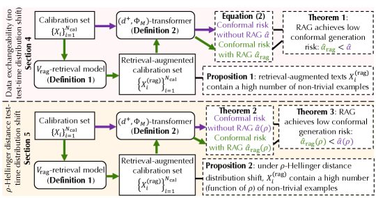
In this section, we prove that RAG model achieves a lower conformal generation risk compared to LLMs without retrievals and its benefits are correlated with the quality of the retrieval model and transformer. We provide the structure of our theoretical analysis and conclusions in Figure 2.
Refer to caption
Figure 2: Certification framework of C-RAG. We provide theoretical results with the data exchangeability assumption in Section 4 (upper row) and extend the results to more complex scenarios under test distribution shifts in Section 5 (lower row).

4.1 Analysis setup

For our analysis, paralleling the previous transformer studies by (Von Oswald et al., 2023; Zhang et al., 2023b; Han et al., 2023), we consider a one-layer self-attention transformer parameterized with the embedding matrix WE:𝒱d1:subscript𝑊𝐸maps-to𝒱superscriptsubscript𝑑1W_{E}:{\mathcal{V}}\mapsto{\mathbb{R}}^{d_{1}}, query matrix WQ:d1d2:subscript𝑊𝑄maps-tosuperscriptsubscript𝑑1superscriptsubscript𝑑2W_{Q}:{\mathbb{R}}^{d_{1}}\mapsto{\mathbb{R}}^{d_{2}}, key matrix WK:d1d2:subscript𝑊𝐾maps-tosuperscriptsubscript𝑑1superscriptsubscript𝑑2W_{K}:{\mathbb{R}}^{d_{1}}\mapsto{\mathbb{R}}^{d_{2}}, value matrix WV:d1d2:subscript𝑊𝑉maps-tosuperscriptsubscript𝑑1superscriptsubscript𝑑2W_{V}:{\mathbb{R}}^{d_{1}}\mapsto{\mathbb{R}}^{d_{2}}, projection matrix WP:d2Δ|𝒱|:subscript𝑊𝑃maps-tosuperscriptsubscript𝑑2superscriptΔ𝒱W_{P}:{\mathbb{R}}^{d_{2}}\mapsto\Delta^{|{\mathcal{V}}|}, and treat each instance approximately as a single token. The retrieval-augmented input text then consists of Nragsubscript𝑁ragN_{\text{rag}} retrieved examples and 111 query example. We denote the augmented input text by 𝒒𝒱Nrag+1𝒒superscript𝒱subscript𝑁rag1{\bm{q}}\in{\mathcal{V}}^{N_{\text{rag}}+1}. We categorize pairs of queries 𝒒i,𝒒j(i,j[Nrag+1])subscript𝒒𝑖subscript𝒒𝑗𝑖𝑗delimited-[]subscript𝑁rag1{\bm{q}}_{i},{\bm{q}}_{j}~{}(i,j\in[N_{\text{rag}}+1]) as positive if they convey identical semantic meanings, indicated by g(𝒒i)=g(𝒒j)𝑔subscript𝒒𝑖𝑔subscript𝒒𝑗g({\bm{q}}_{i})=g({\bm{q}}_{j}). In this context, 𝒒isubscript𝒒𝑖{\bm{q}}_{i} can be referred to as a positive example of 𝒒jsubscript𝒒𝑗{\bm{q}}_{j}. Conversely, pairs 𝒒i,𝒒j(i,j[Nrag+1])subscript𝒒𝑖subscript𝒒𝑗𝑖𝑗delimited-[]subscript𝑁rag1{\bm{q}}_{i},{\bm{q}}_{j}~{}(i,j\in[N_{\text{rag}}+1]) are considered negative if they are semantically different. We use such a definition for clear interpretation of our findings, but our analysis can be extended to include broader definitions of positive pairs, as addressed in the remarks of Theorem 1.

Following the single-layer transformer formulation in (Von Oswald et al., 2023), given an input text 𝒒𝒒{\bm{q}}, we consider the single-token output O(rag)(𝒒)Δ|𝒱|superscript𝑂(rag)𝒒superscriptΔ𝒱O^{\text{(rag)}}({\bm{q}})\in\Delta^{|{\mathcal{V}}|} corresponding to the query example 𝒒Nrag+1subscript𝒒subscript𝑁rag1{\bm{q}}_{N_{\text{rag}+1}} at the last position, formulated as:

O(rag)(𝒒)=σ(WPWV{WE𝒒Nrag+1+(WE𝒒)σ((WKWE𝒒)TWQWE𝒒Nrag+1)}),superscript𝑂(rag)𝒒𝜎subscript𝑊𝑃subscript𝑊𝑉subscript𝑊𝐸subscript𝒒subscript𝑁rag1subscript𝑊𝐸𝒒𝜎superscriptsubscript𝑊𝐾subscript𝑊𝐸𝒒𝑇subscript𝑊𝑄subscript𝑊𝐸subscript𝒒subscript𝑁rag1\displaystyle O^{\text{(rag)}}({\bm{q}})=\sigma\left(W_{P}W_{V}\left\{W_{E}{\bm{q}}_{N_{\text{rag}+1}}+(W_{E}{\bm{q}})\sigma\left((W_{K}W_{E}{\bm{q}})^{T}W_{Q}W_{E}{\bm{q}}_{N_{\text{rag}+1}}\right)\right\}\right), (3)

where σ()𝜎\sigma(\cdot) is the Softmax function. Note that without RAG, the output probability vector O(𝒒)𝑂𝒒O({\bm{q}}) is formulated as O(𝒒)=σ(WPWVWE𝒒Nrag+1)𝑂𝒒𝜎subscript𝑊𝑃subscript𝑊𝑉subscript𝑊𝐸subscript𝒒subscript𝑁rag1O({\bm{q}})=\sigma\left(W_{P}W_{V}W_{E}{\bm{q}}_{N_{\text{rag}+1}}\right).

4.2 Retrieval quality analysis

To quantify the quality of retrieval models, we introduce the concept of Vragsubscript𝑉ragV_{\text{rag}}-retrieval model, where Vragsubscript𝑉ragV_{\text{rag}} measures the variance of the contrastive loss of the retrieval model. A small Vragsubscript𝑉ragV_{\text{rag}} implies a well-trained low-variance retrieval model and can be theoretically linked to the retrieval quality, which is measured by the number of retrieved positive examples with respect to the query text.

Definition 1 (Vragsubscript𝑉ragV_{\text{rag}}-retrieval model).

Consider a retrieval model with similarity measurement sθr(,)subscript𝑠subscript𝜃𝑟s_{\theta_{r}}(\cdot,\cdot) parameterized with θrsubscript𝜃𝑟\theta_{r} and trained with contrastive loss contsubscriptcont{\mathcal{L}}_{\text{cont}}. Let x+,xsuperscript𝑥superscript𝑥x^{+},x^{-} be positive and negative samples to sample x𝑥x. Consider common contrastive loss cont=log(σsig(exp{sθ(x,x)exp{sθ(x,x+))){\mathcal{L}}_{\text{cont}}=-\log\left(\sigma_{\text{sig}}(\exp\{s_{\theta}(x,x^{-})-\exp\{s_{\theta}(x,x^{+}))\right), where σsig()subscript𝜎sig\sigma_{\text{sig}}(\cdot) is the sigmoid function. We define a Vragsubscript𝑉ragV_{\text{rag}}-retrieval model as the retrieval model with (a) a non-trivial utility such that the expected contrastive loss Lτsubscript𝐿𝜏L_{\tau} is better than random: Lτ:=𝔼[cont]<ln2assignsubscript𝐿𝜏𝔼delimited-[]subscriptcont2L_{\tau}:=\mathbb{E}[{\mathcal{L}}_{\text{cont}}]<\ln 2 (i.e., 𝔼[sθ(x,x+)sθ(x,x)]>0𝔼delimited-[]subscript𝑠𝜃𝑥superscript𝑥subscript𝑠𝜃𝑥superscript𝑥0\mathbb{E}[s_{\theta}(x,x^{+})-s_{\theta}(x,x^{-})]>0); and (b) bounded variance such that the training is stable and converges well: Vrag:=𝕍[sθ(x,x+)sθ(x,x)]1/2log(exp{Lτ}1)<1assignsubscript𝑉rag𝕍superscriptdelimited-[]subscript𝑠𝜃𝑥superscript𝑥subscript𝑠𝜃𝑥superscript𝑥12subscript𝐿𝜏11V_{\text{rag}}:={\mathbb{V}[s_{\theta}(x,x^{+})-s_{\theta}(x,x^{-})]^{1/2}}{\log(\exp\{L_{\tau}\}-1)}<1

Remarks.

(R1) Note that a retrieval model with random initialization can achieve 𝔼[sθ(x,x+)]=𝔼[sθ(x,x)]𝔼delimited-[]subscript𝑠𝜃𝑥superscript𝑥𝔼delimited-[]subscript𝑠𝜃𝑥superscript𝑥\mathbb{E}[s_{\theta}(x,x^{+})]=\mathbb{E}[s_{\theta}(x,x^{-})] asymptotically. We merely assume a Vragsubscript𝑉ragV_{\text{rag}}-retrieval model that can non-trivially differentiate the positive from negative examples. (R2) We also assume a moderate stability with bounded variance, which implicitly assumes a moderate generalization of the retrieval model based on the variance-generalization link (Lam, 2016; Gotoh et al., 2018; Namkoong & Duchi, 2017). This is essential for the analysis as the knowledge base distribution is non-identical to the calibration/test distribution. (R3) We define Vragsubscript𝑉ragV_{\text{rag}}-retrieval model using a standard contrastive loss in (Wang et al., 2023b; Rubin et al., 2021), but it can be adapted for other contrastive loss such as triplet loss (Hermans et al., 2017), by altering the logarithmic factor in the Vragsubscript𝑉ragV_{\text{rag}} formula. We defer the proof sketches as well as the detailed proofs and remarks to Appendix F.

With a Vragsubscript𝑉ragV_{\text{rag}}-retrieval model, we show that C-RAG can retrieve a high number of positive examples as in-context demonstrations as follows.

Proposition 3 (lower bound of the number of retrieved positive examples).

Consider the Vragsubscript𝑉ragV_{\text{rag}}-retrieval model in Definition 1 and RAG generation protocol in Section 3.2. Let rcal(c)subscriptsuperscript𝑟𝑐calr^{(c)}_{\text{cal}} and rext(c)subscriptsuperscript𝑟𝑐extr^{(c)}_{\text{ext}} be the portion of data with groundtruth output c𝒴𝑐𝒴c\in{\mathcal{Y}} in the calibration data distribution and external knowledge data distribution, respectively. We have:

𝔼[Npos]𝔼delimited-[]subscript𝑁posabsent\displaystyle\mathbb{E}\left[N_{\text{pos}}\right]\geq 910Nrag(1c𝒴rcal(c)(Nextrext(c)Next+2ln10)Vrag0.5(rext(c)Next2ln10))910subscript𝑁rag1subscript𝑐𝒴subscriptsuperscript𝑟𝑐calsubscript𝑁extsubscriptsuperscript𝑟𝑐extsubscript𝑁ext210superscriptsubscript𝑉rag0.5subscriptsuperscript𝑟𝑐extsubscript𝑁ext210\displaystyle\dfrac{9}{10}N_{\text{rag}}\big{(}1-\sum_{c\in{\mathcal{Y}}}r^{(c)}_{\text{cal}}\left(N_{\text{ext}}-r^{(c)}_{\text{ext}}N_{\text{ext}}+{\sqrt{2\ln{10}}}\right)V_{\text{rag}}^{0.5\left(r^{(c)}_{\text{ext}}N_{\text{ext}}-{\sqrt{2\ln{10}}}\right)}\big{)} (4)

where Npossubscript𝑁posN_{\text{pos}} is the number of retrieved positive examples, Nragsubscript𝑁ragN_{\text{rag}} is the total number of retrieved examples, and Nextsubscript𝑁extN_{\text{ext}} is the number of examples in the external knowledge base.

Remarks.

Proposition 3 offers a guarantee on the minimum number of positive examples retrieved by the Vragsubscript𝑉ragV_{\text{rag}}-retrieval model. (R1) The ratio of the retrieved examples that are positive increases at an exponential rate with respect to Nextsubscript𝑁extN_{\text{ext}}, which suggests that expanding the external knowledge base could enhance the retrieval quality and therefore benefit in-context learning of LLMs, as shown in (Min et al., 2022; Wang et al., 2022a). For a sufficiently large Nextsubscript𝑁extN_{\text{ext}} (a common scenario in practice), the lower bound approximately scales with 0.9Nrag0.9subscript𝑁rag0.9N_{\text{rag}}. (R2) If the knowledge base is highly long-tailed such that samples of certain reference texts are rare (i.e., small rext(c)superscriptsubscript𝑟ext𝑐r_{\text{ext}}^{(c)}), we require a larger sample size of knowledge base Nextsubscript𝑁extN_{\text{ext}} to compensate for the long-tail distribution and achieve comparable retrieval quality. (R3) A low-variance retrieval model is expected to generalize well to test distribution and increase retrieval quality. The above guarantee we provide for 𝔼[Npos]𝔼delimited-[]subscript𝑁pos\mathbb{E}[N_{\text{pos}}] in relation to Vragsubscript𝑉ragV_{\text{rag}} is a rigorous demonstration of this.

4.3 RAG achieves provably lower conformal generation risk than a single LLM without retrieval

Besides retrieval quality, the generation risk in RAG models is also affected by LLM quality, and to measure transformer quality, we define a (d+,ΦM)superscript𝑑subscriptΦ𝑀(d^{+},\Phi_{M})-transformer as follows.

Definition 2 ((d+,ΦM)superscript𝑑subscriptΦ𝑀(d^{+},\Phi_{M})-transformer).

We assume that each in-context example (Xi,Yi)(i[Nrag+1])subscript𝑋𝑖subscript𝑌𝑖𝑖delimited-[]subscript𝑁rag1(X_{i},Y_{i})~{}(i\in[N_{\text{rag}}+1]) is encoded with a single token 𝒒isubscript𝒒𝑖{\bm{q}}_{i}. Let 𝒒𝒒{\bm{q}} be the retrieval-augmented input, consisting of Nragsubscript𝑁ragN_{\text{rag}} retrieved in-context examples and 111 query example. We define a random variable to represent the negative prediction margin: M=maxcg(𝒒Nrag+1)Oc(𝒒)Og(𝒒Nrag+1)(𝒒)𝑀subscript𝑐𝑔subscript𝒒subscript𝑁rag1subscript𝑂𝑐𝒒subscript𝑂𝑔subscript𝒒subscript𝑁rag1𝒒M=\max_{c\neq g({\bm{q}}_{N_{\text{rag}}+1})}O_{c}({\bm{q}})-O_{g({\bm{q}}_{N_{\text{rag}}+1})}({\bm{q}}), where O(𝒒)𝑂𝒒O({\bm{q}}) is the output probability vector without RAG. Let ΦM()subscriptΦ𝑀\Phi_{M}(\cdot) be the CDF of random variable M𝑀M. We define a (d+,ΦM)superscript𝑑subscriptΦ𝑀(d^{+},\Phi_{M})-transformer as a single-layer self-attention transformer with (a) non-trivial self-attention layer with σ((WKWE𝒒i)T(WQWE𝒒j))d+>0𝜎superscriptsubscript𝑊𝐾subscript𝑊𝐸subscript𝒒𝑖𝑇subscript𝑊𝑄subscript𝑊𝐸subscript𝒒𝑗superscript𝑑0\sigma\left((W_{K}W_{E}{\bm{q}}_{i})^{T}(W_{Q}W_{E}{\bm{q}}_{j})\right)\geq d^{+}>0 for semantically identical examples with g(𝒒i)=g(𝒒j)𝑔subscript𝒒𝑖𝑔subscript𝒒𝑗g({\bm{q}}_{i})=g({\bm{q}}_{j}); and (b) the prediction utility that is better than random: 11ΦM(v)𝑑v>1superscriptsubscript11subscriptΦ𝑀𝑣differential-d𝑣1\int_{-1}^{1}\Phi_{M}(v)dv>1.

Remarks.

(R1) d+superscript𝑑d^{+} measures the minimal attention scores for positive pairs and reflects the effectiveness of the transformer’s embedding, key, and query matrices. Since we always have d+0superscript𝑑0d^{+}\geq 0 due to the Softmax activation, the condition d+>0superscript𝑑0d^{+}>0 only assumes a non-trivial self-attention layer. (R2) The integral 11ΦM(v)𝑑vsuperscriptsubscript11subscriptΦ𝑀𝑣differential-d𝑣\int_{-1}^{1}\Phi_{M}(v)dv measures the quality of the embedding, value, and projection matrices. Note that a random prediction margin Mrandsubscript𝑀randM_{\text{rand}} over a uniform distribution [1,1]11[-1,1] results in 11ΦMrand(v)𝑑v=1superscriptsubscript11subscriptΦsubscript𝑀rand𝑣differential-d𝑣1\int_{-1}^{1}\Phi_{M_{\text{rand}}}(v)dv=1. Thus, 11ΦM(v)𝑑v>1=11ΦMrand(v)𝑑vsuperscriptsubscript11subscriptΦ𝑀𝑣differential-d𝑣1superscriptsubscript11subscriptΦsubscript𝑀rand𝑣differential-d𝑣\int_{-1}^{1}\Phi_{M}(v)dv>1=\int_{-1}^{1}\Phi_{M_{\text{rand}}}(v)dv only indicates better-than-random prediction utility.

Next, we prove that RAG in C-RAG achieves a lower conformal generation risk than a single LLM without retrieval with high probability.

Theorem 1 (RAG reduces the conformal generation risk).

Consider the setup in Section 4.1 as well as the Vragsubscript𝑉ragV_{\text{rag}}-retrieval model in Definition 1 and (d+,ΦM)superscript𝑑subscriptΦ𝑀(d^{+},\Phi_{M})-transformer in Definition 2. Let rcal(c)subscriptsuperscript𝑟𝑐calr^{(c)}_{\text{cal}} and rext(c)subscriptsuperscript𝑟𝑐extr^{(c)}_{\text{ext}} be as defined in Proposition 3. We show that the conformal generation risk of RAG α^ragsubscript^𝛼rag\hat{\alpha}_{\text{rag}} is smaller than that of a single LLM α^^𝛼\hat{\alpha} with high probability:

[α^rag<α^]1ptpr,wheredelimited-[]subscript^𝛼rag^𝛼1subscript𝑝tsubscript𝑝rwhere\displaystyle{\mathbb{P}}\left[\hat{\alpha}_{\text{rag}}<\hat{\alpha}\right]\geq 1-p_{\text{t}}-p_{\text{r}},\quad\text{where} (5)
pt=exp{2Ncal[ΦM(12d+(11ΦM(v)𝑑v1)quality of transformersNrag)ΦM(0)improvement of generation quality with RAG]2}subscript𝑝t2subscript𝑁calsuperscriptdelimited-[]subscriptsubscriptΦ𝑀12superscriptsuperscript𝑑superscriptsubscript11subscriptΦ𝑀𝑣differential-d𝑣1quality of transformerssubscript𝑁ragsubscriptΦ𝑀0improvement of generation quality with RAG2\displaystyle p_{\text{t}}=\exp\{-2N_{\text{cal}}[\underbrace{\Phi_{M}(\dfrac{1}{2}{\overbrace{d^{+}(\int_{-1}^{1}\Phi_{M}(v)dv-1)}^{\text{quality of transformers}}}N_{\text{rag}})-\Phi_{M}(0)}_{\text{improvement of generation quality with RAG}}]^{2}\}
pr=25Nrag(49c=1Crcal(c)(1.5Nextrext(c)Next)Vrag0.25rext(c)Nextnumber of retrieved negative examples)2subscript𝑝r25subscript𝑁ragsuperscript49subscriptsuperscriptsubscript𝑐1𝐶subscriptsuperscript𝑟𝑐cal1.5subscript𝑁extsubscriptsuperscript𝑟𝑐extsubscript𝑁extsuperscriptsubscript𝑉rag0.25subscriptsuperscript𝑟𝑐extsubscript𝑁extnumber of retrieved negative examples2\displaystyle p_{\text{r}}=\dfrac{25}{N_{\text{rag}}}(4-9\underbrace{\sum_{c=1}^{C}r^{(c)}_{\text{cal}}(1.5N_{\text{ext}}-r^{(c)}_{\text{ext}}N_{\text{ext}})V_{\text{rag}}^{0.25r^{(c)}_{\text{ext}}N_{\text{ext}}}}_{\text{number of retrieved negative examples}})^{-2}

provided that Next>22ln10/mincrext(c)subscript𝑁ext2210subscript𝑐superscriptsubscript𝑟ext𝑐\footnotesize{N_{\text{ext}}>{2\sqrt{2\ln 10}}/{\min_{c}r_{\text{ext}}^{(c)}}}, Nrag>2/d+subscript𝑁rag2superscript𝑑N_{\text{rag}}>{2}/{d^{+}} and NextVrag0.25mincrext(c)Next<4/9subscript𝑁extsuperscriptsubscript𝑉rag0.25subscript𝑐superscriptsubscript𝑟ext𝑐subscript𝑁ext49\footnotesize{N_{\text{ext}}V_{\text{rag}}^{0.25\min_{c}r_{\text{ext}}^{(c)}N_{\text{ext}}}<{4}/{9}}. pt,prsubscript𝑝𝑡subscript𝑝𝑟p_{t},p_{r} are the uncertainty induced by the quality of transformer and retrieval model.

Remarks.

(R1) The probability of reduced risk with RAG ([α^rag<α^]delimited-[]subscript^𝛼rag^𝛼{\mathbb{P}}\left[\hat{\alpha}_{\text{rag}}<\hat{\alpha}\right]) increases with both Ncalsubscript𝑁calN_{\text{cal}}, which improves risk approximation via enhanced calibration, and Nragsubscript𝑁ragN_{\text{rag}} and Nextsubscript𝑁extN_{\text{ext}}, which expand the scope of retrieved knowledge. (R2) The reduced risk probability also increases with the transformer’s quality induced by attention scores and prediction capability. (R3) A low-variance retrieval model (small Vragsubscript𝑉ragV_{\text{rag}}) enhances generalization and reduces retrieval model uncertainty prsubscript𝑝𝑟p_{r}. (R4) For certification simplicity, we define positive pairs as semantically identical examples, but this can be expanded to pairs similar in the embedding space for boosting attention scores, in-context learning, and generation quality. (R5) These result can readily extend to various conformal risks such as (Angelopoulos et al., 2022). (R6) For sufficiently large sample size Nextsubscript𝑁extN_{\text{ext}} in the external knowledge base, we further have [α^rag<α^]1pt25/16Nragdelimited-[]subscript^𝛼rag^𝛼1subscript𝑝𝑡2516subscript𝑁rag{\mathbb{P}}\left[\hat{\alpha}_{\text{rag}}<\hat{\alpha}\right]\geq 1-p_{t}-{25}/{16N_{\text{rag}}} (Corollary 1 in Appendix G). In contrast to Theorem 1, the bound has no dependency on the external knowledge distribution rext(c)superscriptsubscript𝑟ext𝑐r_{\text{ext}}^{(c)} and calibration distribution rcal(c)superscriptsubscript𝑟cal𝑐r_{\text{cal}}^{(c)}.

5 C-RAG under distribution shifts

Here, we present a valid distribution-drift conformal generation risk and prove the benefit of RAG compared to vanilla LLM under test-time distribution shifts.

5.1 Analysis setup

Conformal risk guarantees often assume that calibration and testing samples come from the same distribution (Bates et al., 2021; Angelopoulos et al., 2022, 2021). Next, building on Section 4.1, we extend these guarantees to distribution shifts between calibration and testing.

5.2 Conformal generation risk under distribution shifts

Under test-time distribution shifts, the certification guarantees of prior work (Angelopoulos et al., 2022; Farinhas et al., 2023a) are limited to the monotonic risk functions and to distribution shifts caused by changes in sample weights. Here, we provide generation risk certification for any bounded risk function and any distribution shift, which is as follows.

Theorem 2 (Conformal generation risk under distribution shifts).

Suppose that the test instance (Xtest,Ytest)subscript𝑋testsubscript𝑌test(X_{\text{test}},Y_{\text{test}}) is sampled from a shifted distribution 𝒬𝒬{\mathcal{Q}} with bounded Hellinger distance from the calibration distribution 𝒟𝒟{\mathcal{D}}: H(𝒟,𝒬)ρ𝐻𝒟𝒬𝜌H({\mathcal{D}},{\mathcal{Q}})\leq\rho. Let R^=i=1NcalR(Zi)/Ncal^𝑅superscriptsubscript𝑖1subscript𝑁cal𝑅subscript𝑍𝑖subscript𝑁cal\hat{R}=\sum_{i=1}^{N_{\text{cal}}}R(Z_{i})/N_{\text{cal}} be the empirical risk on calibration samples Zi(i{1,,Ncal})subscript𝑍𝑖𝑖1subscript𝑁calZ_{i}~{}(i\in\{1,...,N_{\text{cal}}\}) and V^=1/Ncal(Ncal1)1i<jNcal(R(Zi)R(Zj))2^𝑉1subscript𝑁calsubscript𝑁cal1subscript1𝑖𝑗subscript𝑁calsuperscript𝑅subscript𝑍𝑖𝑅subscript𝑍𝑗2\hat{V}={1}/{N_{\text{cal}}(N_{\text{cal}}-1)}\sum_{1\leq i<j\leq N_{\text{cal}}}(R(Z_{i})-R(Z_{j}))^{2} be the unbiased estimator of the risk variance on the calibration set. Then we have the following guarantee of conformal generation risk on the shifted distribution 𝒬𝒬{\mathcal{Q}}:

[R(T𝝀^;Xtest,Ytest)α^(ρ)]1δ,whereα^(ρ):=min{h1(8/δNcal;R^ρ¯),Φbin1(δ8e;Ncal,R^ρ¯)}formulae-sequencedelimited-[]𝑅subscript𝑇^𝝀subscript𝑋testsubscript𝑌test^𝛼𝜌1𝛿whereassign^𝛼𝜌superscript18𝛿subscript𝑁cal¯subscript^𝑅𝜌subscriptsuperscriptΦ1bin𝛿8𝑒subscript𝑁cal¯subscript^𝑅𝜌\displaystyle{\mathbb{P}}\left[R(T_{\hat{{\bm{\lambda}}}};X_{\text{test}},Y_{\text{test}})\leq\hat{\alpha}(\rho)\right]\geq 1-\delta,\quad\text{where}\quad\hat{\alpha}(\rho):=\min\left\{h^{-1}\left(\dfrac{8/\delta}{N_{\text{cal}}};\overline{\hat{R}_{\rho}}\right),\Phi^{-1}_{\text{bin}}\left(\dfrac{\delta}{8e};N_{\text{cal}},\overline{\hat{R}_{\rho}}\right)\right\} (6)

where h1(;)superscript1h^{-1}(\cdot;\cdot) is the partial inverse function as defined in Proposition 1 and R^ρ¯¯subscript^𝑅𝜌\overline{\hat{R}_{\rho}} is formulated as:

R^ρ¯=R^+ρ2(2ρ2)(1R^)empirical mean scaled by ρ+2ρ(1ρ2)2ρ2V^estimated variance scaled by ρ+(1ρ2)(1ρ22Ncal+22ρ2ρ2Ncal1)ln(4/δ)+ln(8/δ)2Ncalfinite-sample error¯subscript^𝑅𝜌subscript^𝑅superscript𝜌22superscript𝜌21^𝑅empirical mean scaled by 𝜌subscript2𝜌1superscript𝜌22superscript𝜌2^𝑉estimated variance scaled by 𝜌subscript1superscript𝜌21superscript𝜌22subscript𝑁cal22𝜌2superscript𝜌2subscript𝑁cal14𝛿8𝛿2subscript𝑁calfinite-sample error\displaystyle\overline{\hat{R}_{\rho}}=\underbrace{\hat{R}+\rho^{2}(2-\rho^{2})(1-\hat{R})}_{\text{empirical mean scaled by }\rho}+\underbrace{2\rho(1-\rho^{2})\sqrt{2-\rho^{2}}\sqrt{\hat{V}}}_{\text{estimated variance scaled by }\rho}+\underbrace{(1-\rho^{2})\left(\dfrac{1-\rho^{2}}{\sqrt{2N_{\text{cal}}}}+\dfrac{2\sqrt{2}\rho\sqrt{2-\rho^{2}}}{\sqrt{N_{\text{cal}}-1}}\right)\sqrt{\ln(4/\delta)}+\sqrt{\dfrac{\ln{(8/\delta)}}{2N_{\text{cal}}}}}_{\text{finite-sample error}}

where the radius ρ𝜌\rho satisfies the following: ρ21[1+(R^1+ln(4/δ)/2Ncal)2/(V^+2ln(2/δ)/(Ncal1))2]2\rho^{2}\leq 1-\big{[}1+\big{(}\nicefrac{{\hat{R}-1+\sqrt{\nicefrac{{\ln(4/\delta)}}{{2N_{\text{cal}}}}}\big{)}^{2}}}{{\big{(}\sqrt{\hat{V}}+\sqrt{\nicefrac{{2\ln(2/\delta)}}{{(N_{\text{cal}}-1)}}}\big{)}^{2}}}\big{]}^{-2}.

Remarks.

Theorem 2 offers a distribution-drift conformal generation risk α^(ρ)^𝛼𝜌\hat{\alpha}(\rho), under the distribution shift with radius ρ𝜌\rho. (R1) We adopt the Hellinger distance for measuring distribution distances due to its f-divergence properties and direct applicability to total variation distance between 𝒟𝒟{\mathcal{D}} and 𝒬𝒬{\mathcal{Q}} ((Steerneman, 1983), Equation 1). (R2) For conformal guarantees under distribution shifts, we derive an empirical risk upper bound considering worst-case shifts in Theorem 2, which is efficiently calculable with empirical statistics on calibration distribution 𝒟𝒟{\mathcal{D}}. (R3) We recover the empirical mean R^^𝑅\hat{R} from R^ρ¯¯subscript^𝑅𝜌\overline{\hat{R}_{\rho}} when ρ0𝜌0\rho\rightarrow 0 and Ncalsubscript𝑁calN_{\text{cal}}\rightarrow\infty in Theorem 2.

5.3 RAG achieves provably lower conformal generation risk than a single LLM under distribution shifts

Next, we prove that RAG mitigates conformal generation risk better than a single LLM under distribution shifts.111Additionally, we examine retrieval quality and prove a lower bound of retrieved positive examples under test-time distribution shifts. We leave the analysis to Appendix H for interested readers.

Theorem 3 (RAG reduces conformal generation risk even under distribution shifts).

Suppose that the shifted test distribution 𝒬𝒬{\mathcal{Q}} is within bounded Hellinger distance ρ>0𝜌0\rho>0 to the calibration distribution 𝒟𝒟{\mathcal{D}}. Consider the same setup and assumptions as Theorem 1. Consider also a Vragsubscript𝑉ragV_{\text{rag}}-retrieval model in Definition 1 and (d+,ΦM)superscript𝑑subscriptΦ𝑀(d^{+},\Phi_{M})-transformer in Definition 2. Under the condition that Next>22ln10/rextmsubscript𝑁ext2210superscriptsubscript𝑟ext𝑚N_{\text{ext}}>{2\sqrt{2\ln 10}}/{r_{\text{ext}}^{m}}, NextVrag(ρ)0.25rextmNext<8/17subscript𝑁extsubscript𝑉ragsuperscript𝜌0.25superscriptsubscript𝑟ext𝑚subscript𝑁ext817N_{\text{ext}}V_{\text{rag}}(\rho)^{0.25r_{\text{ext}}^{m}N_{\text{ext}}}<{8}/{17}, and Nrag>2/d+subscript𝑁rag2superscript𝑑N_{\text{rag}}>{2}/{d^{+}} , we have:

[α^rag(ρ)<α(ρ)]1ptpr(ρ),wherepr(ρ)=100Nrag(817NextVrag(ρ)0.25(mincrext(c)Next))2,formulae-sequencedelimited-[]subscript^𝛼rag𝜌𝛼𝜌1subscript𝑝𝑡subscript𝑝𝑟𝜌wheresubscript𝑝𝑟𝜌100subscript𝑁ragsuperscript817subscript𝑁extsubscript𝑉ragsuperscript𝜌0.25subscript𝑐subscriptsuperscript𝑟𝑐extsubscript𝑁ext2\displaystyle{\mathbb{P}}\left[\hat{\alpha}_{\text{rag}}(\rho)<\alpha(\rho)\right]\geq 1-p_{t}-p_{r}(\rho),\quad\text{where}\quad p_{r}(\rho)=\dfrac{100}{N_{\text{rag}}}\left(8-17N_{\text{ext}}V_{\text{rag}}(\rho)^{0.25\left(\min_{c}r^{(c)}_{\text{ext}}N_{\text{ext}}\right)}\right)^{-2}, (7)

where ptsubscript𝑝tp_{\text{t}} is the uncertainty induced by the transformer quality as Equation 5 and pr(ρ)subscript𝑝𝑟𝜌p_{r}(\rho) is the uncertainty induced by the retrieval model. Moreover, Vrag(ρ)=m(ρ)Vragsubscript𝑉rag𝜌𝑚𝜌subscript𝑉ragV_{\text{rag}}(\rho)=m(\rho)V_{\text{rag}} quantifies the quality of retrieval models under distance ρ𝜌\rho, where

Vrag(ρ):=m(ρ)Vrag,wherem(ρ)=(6ρ4+12ρ2+14ρ(1ρ2)2ρ2116ρ2+8ρ4)2retrieval model quality decay factor under distribution shifts.formulae-sequenceassignsubscript𝑉rag𝜌𝑚𝜌subscript𝑉ragwhere𝑚𝜌subscriptsuperscript6superscript𝜌412superscript𝜌214𝜌1superscript𝜌22superscript𝜌2116superscript𝜌28superscript𝜌42retrieval model quality decay factor under distribution shifts\displaystyle\vspace{-1em}V_{\text{rag}}(\rho):=m(\rho)V_{\text{rag}},\quad\text{where}\quad m(\rho)=\underbrace{\left(\dfrac{\sqrt{-6\rho^{4}+12\rho^{2}+1}-4\rho(1-\rho^{2})\sqrt{2-\rho^{2}}}{1-16\rho^{2}+8\rho^{4}}\right)^{-2}}_{\text{retrieval model quality decay factor under distribution shifts}}.
Remarks.

Our result rigorously characterizes the effect of distribution shift on the reduced risk guarantee of RAG. (R1) Compared to Theorem 1, only the uncertainty of retrieval model pr(ρ)subscript𝑝𝑟𝜌p_{r}(\rho) is affected by the distribution shift ρ𝜌\rho. This affect is reflected on the the retrieval quality Vrag(ρ)subscript𝑉rag𝜌V_{\text{rag}}(\rho). In particular, a large distance radius ρ𝜌\rho will downgrade the retrieval quality Vrag(ρ)subscript𝑉rag𝜌V_{\text{rag}}(\rho) and thus lead to a higher uncertainty pr(ρ)subscript𝑝𝑟𝜌p_{r}(\rho). However, the influence of ρ𝜌\rho on pr(ρ)subscript𝑝𝑟𝜌p_{r}(\rho) can be reduced by Nragsubscript𝑁ragN_{\text{rag}} inverse proportionally and by Nextsubscript𝑁extN_{\text{ext}} exponentially, demonstrating the robustness of RAG with more retrieval knowledge. (R2) Since Vrag(ρ)subscript𝑉rag𝜌V_{\text{rag}}(\rho) is proportional to model variance Vragsubscript𝑉ragV_{\text{rag}}, a low-variance retrieval model demonstrates better robustness against distribution drifts, aligning with existing empirical observations (Lam, 2016; Gotoh et al., 2018; Namkoong & Duchi, 2017), which evaluate the generalization ability of low-variance retrieval models under distribution shifts. (R3) Compared to Theorem 1, Theorem 3 has no dependence on varying label portions rcal(c)subscriptsuperscript𝑟𝑐calr^{(c)}_{\text{cal}} during distribution shifts, as long as the size of external knowledge base Nextsubscript𝑁extN_{\text{ext}} is moderately large, a condition often met in practice with large knowledge bases.

 AESLC
Refer to caption

Generation risk

 CommonGen

Refer to caption

 DART

Refer to caption

 E2E

Refer to caption

Generation risk

Refer to caption

Refer to caption

Refer to caption

Refer to caption

Generation risk

Refer to caption

Refer to caption

Refer to caption

Refer to caption

Refer to caption

   # Retrieved examples Nragsubscript𝑁ragN_{\text{rag}}

Generation risk

Refer to caption

   # Retrieved examples Nragsubscript𝑁ragN_{\text{rag}}

Refer to caption

   # Retrieved examples Nragsubscript𝑁ragN_{\text{rag}}

Refer to caption

   # Retrieved examples Nragsubscript𝑁ragN_{\text{rag}}

Refer to caption

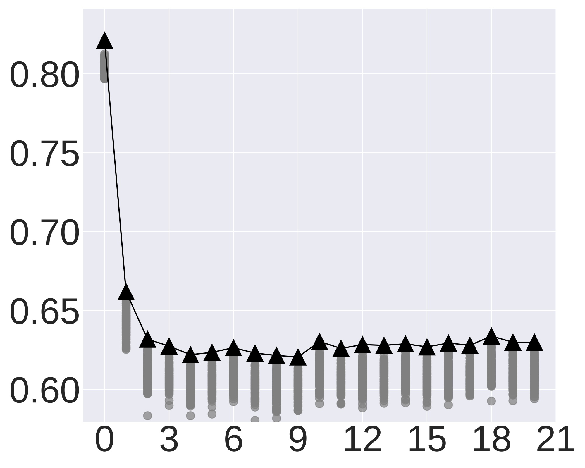
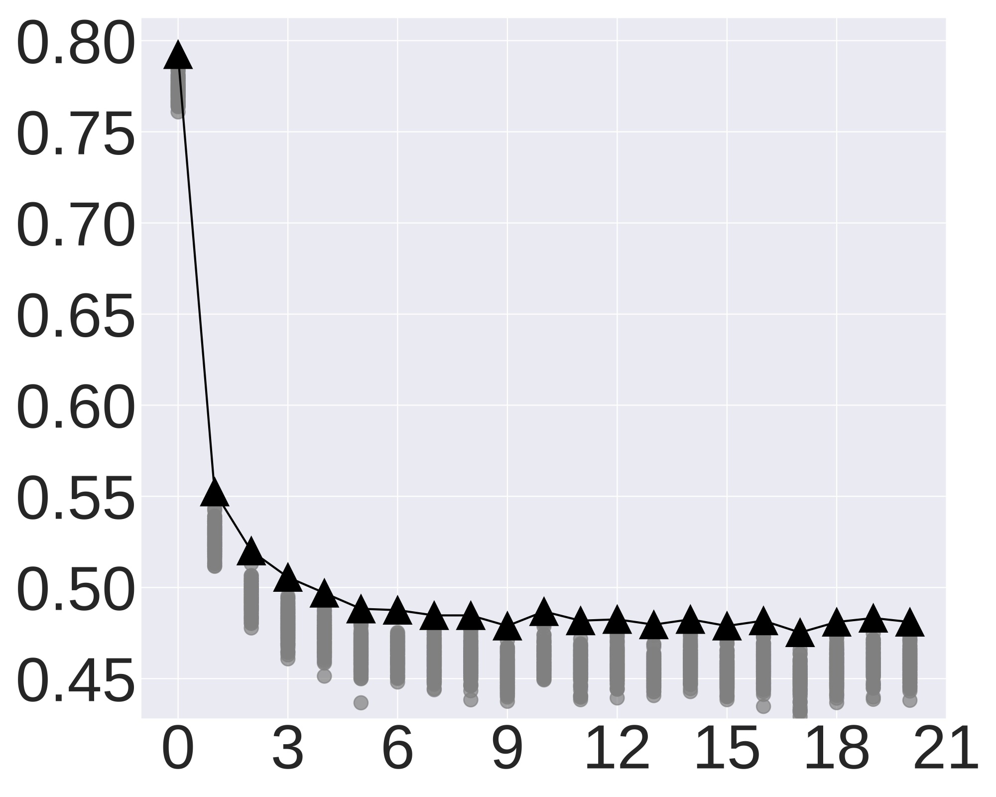
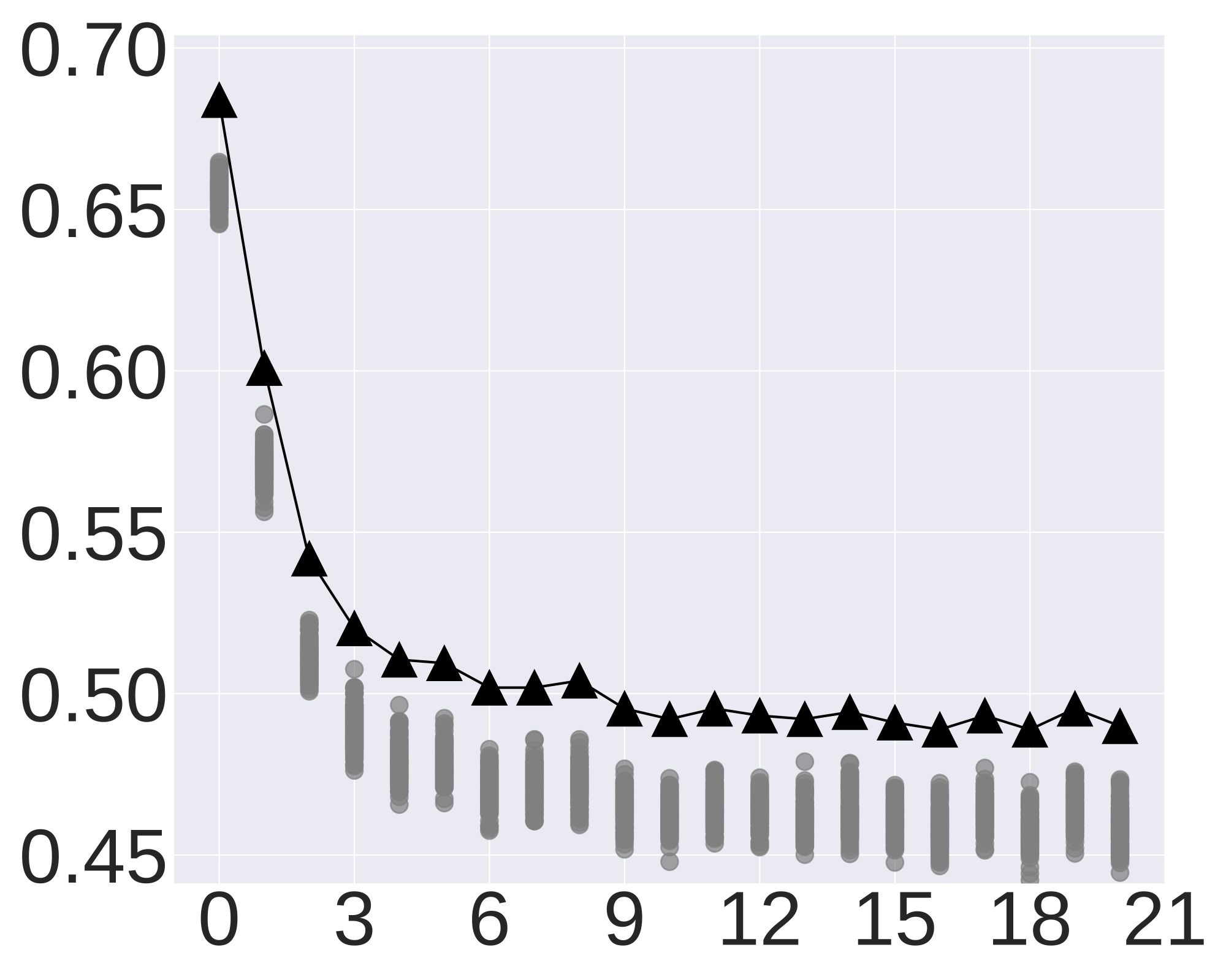
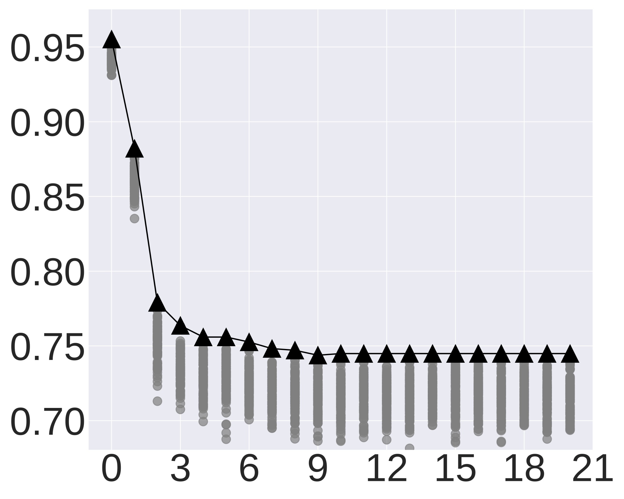
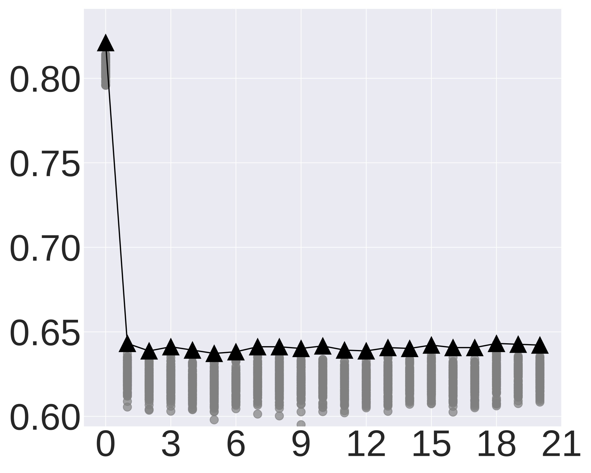
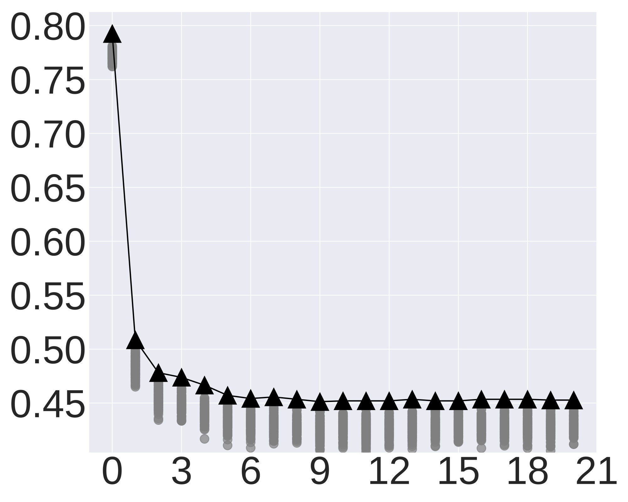
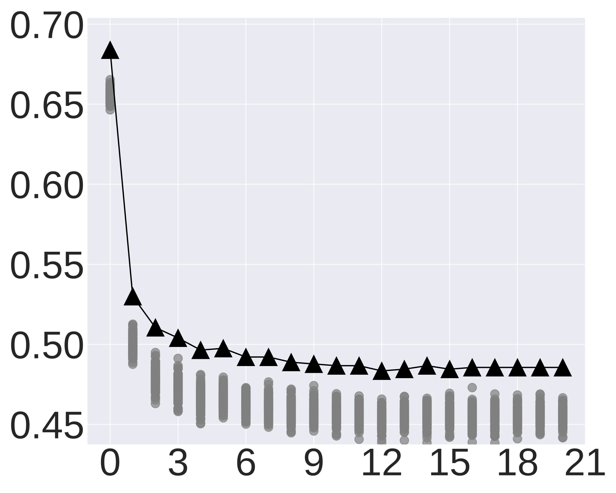
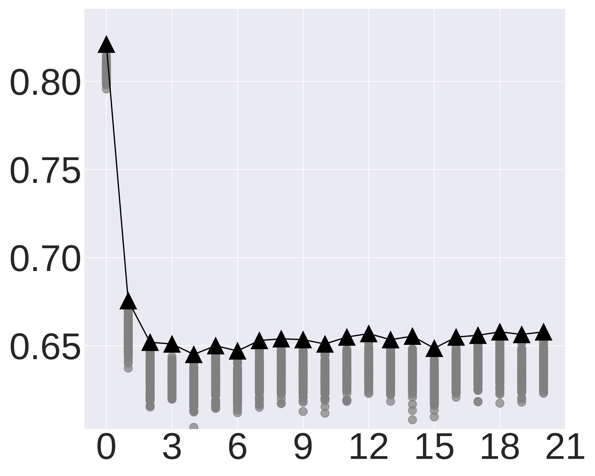
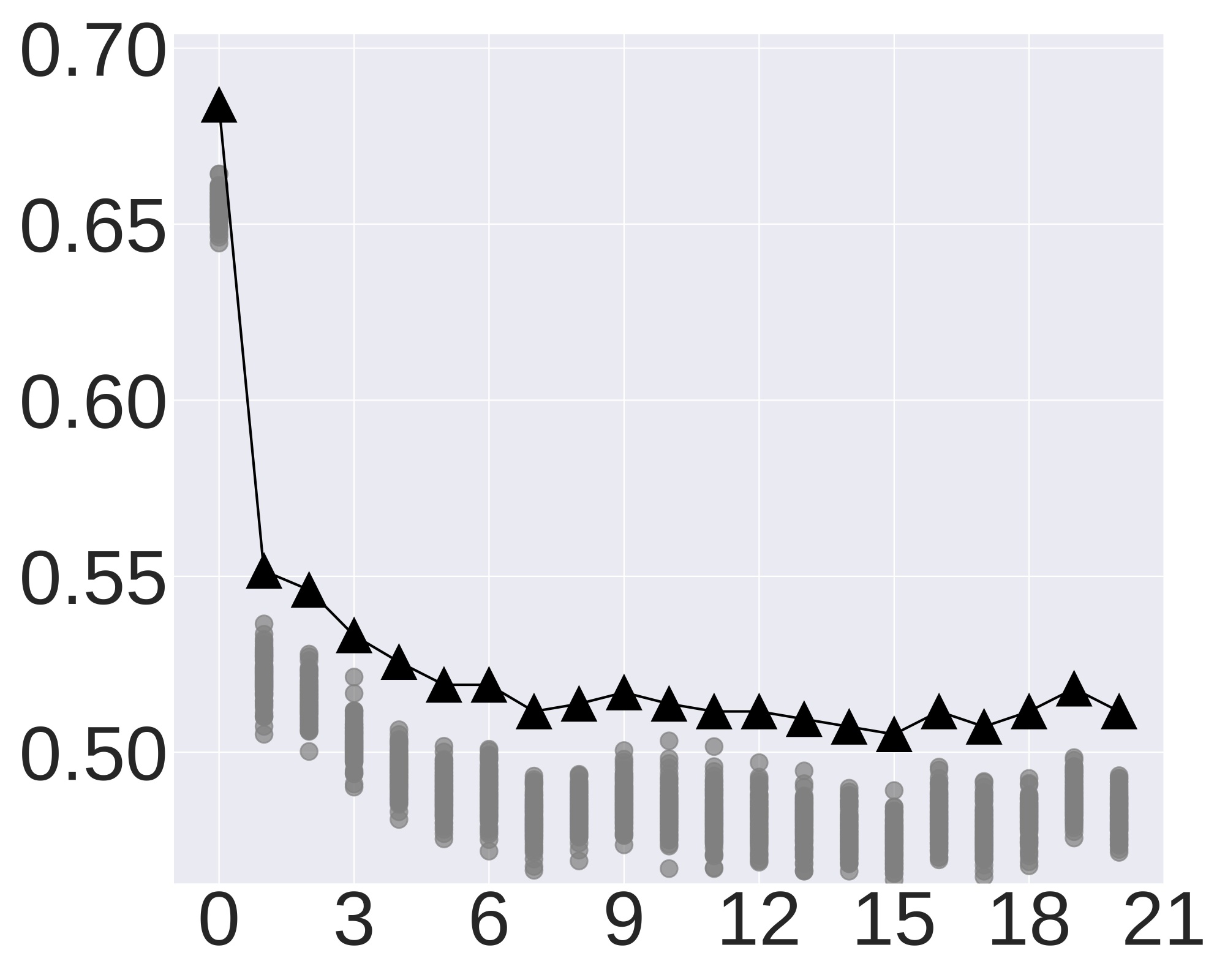
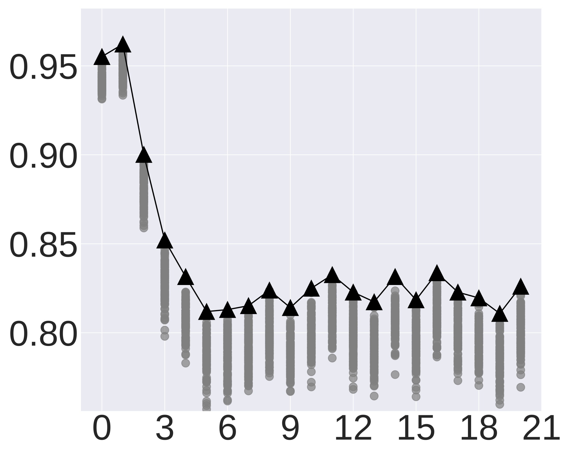
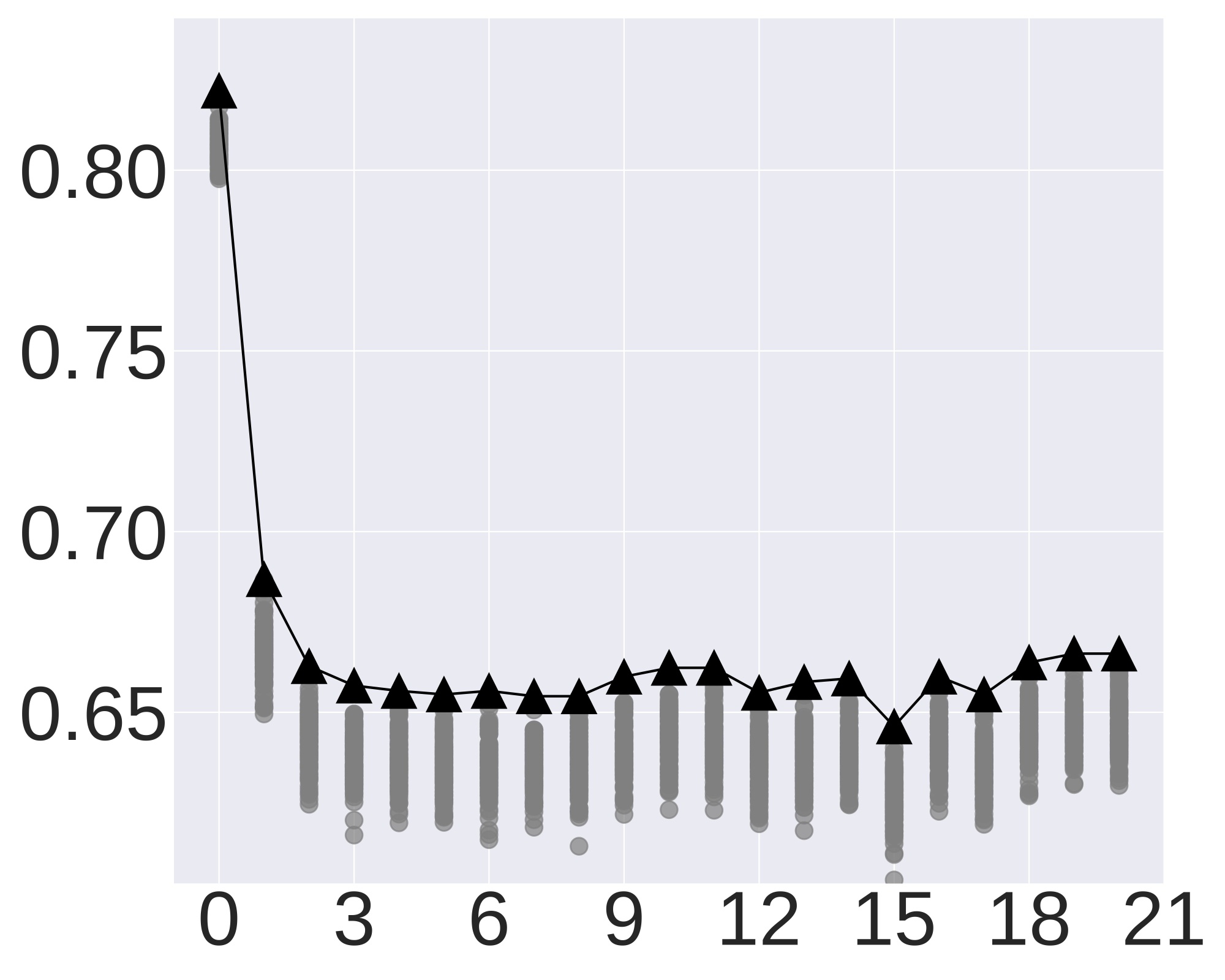
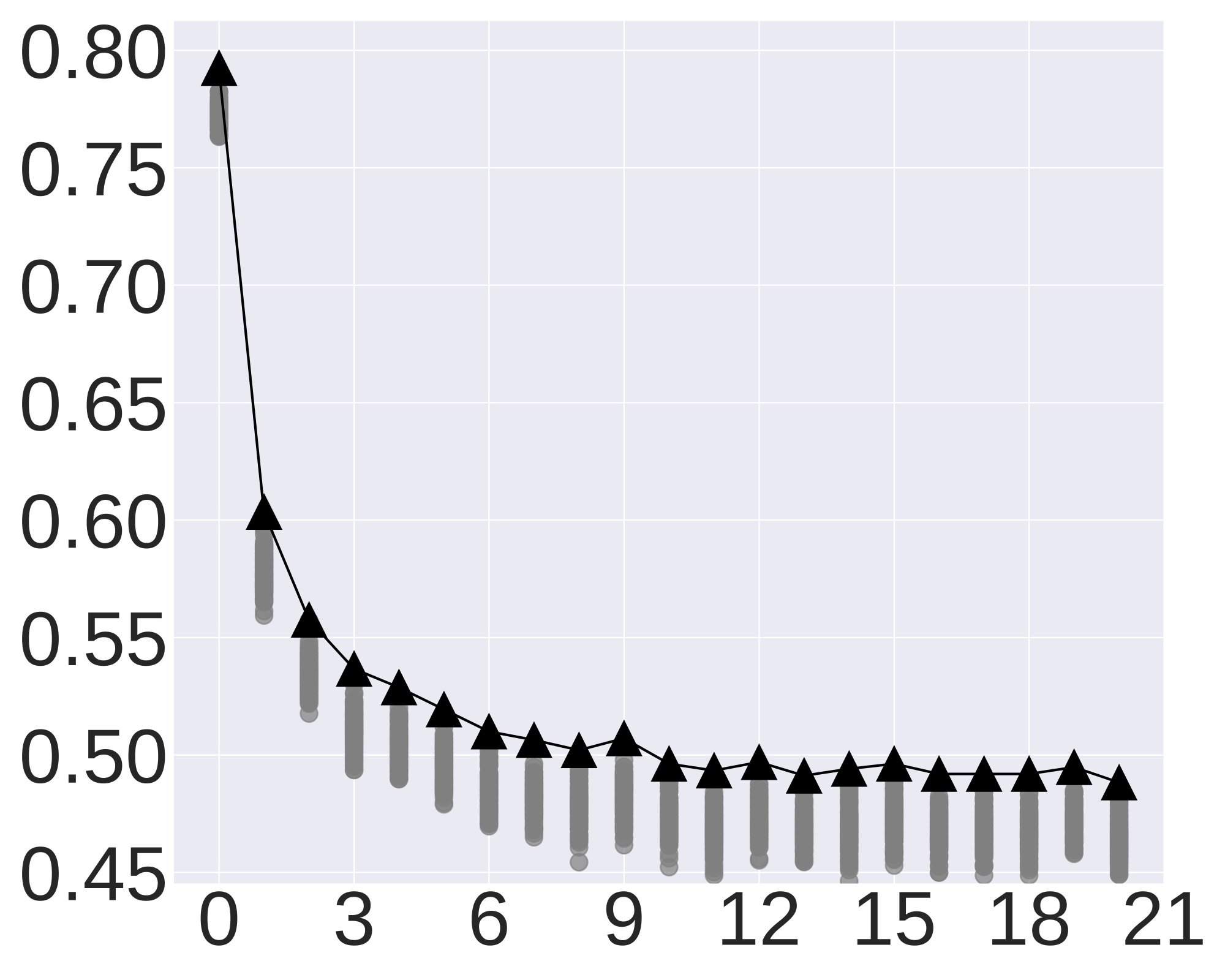
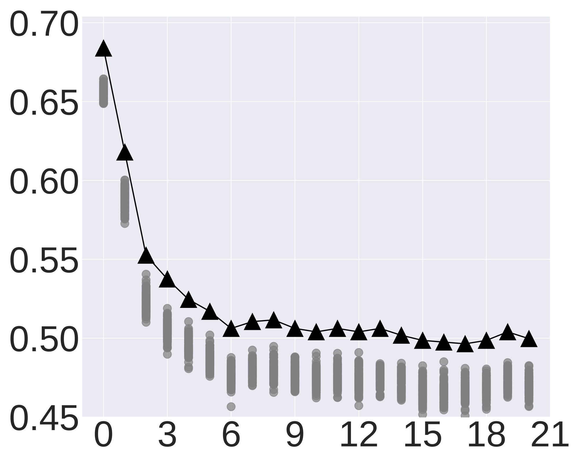
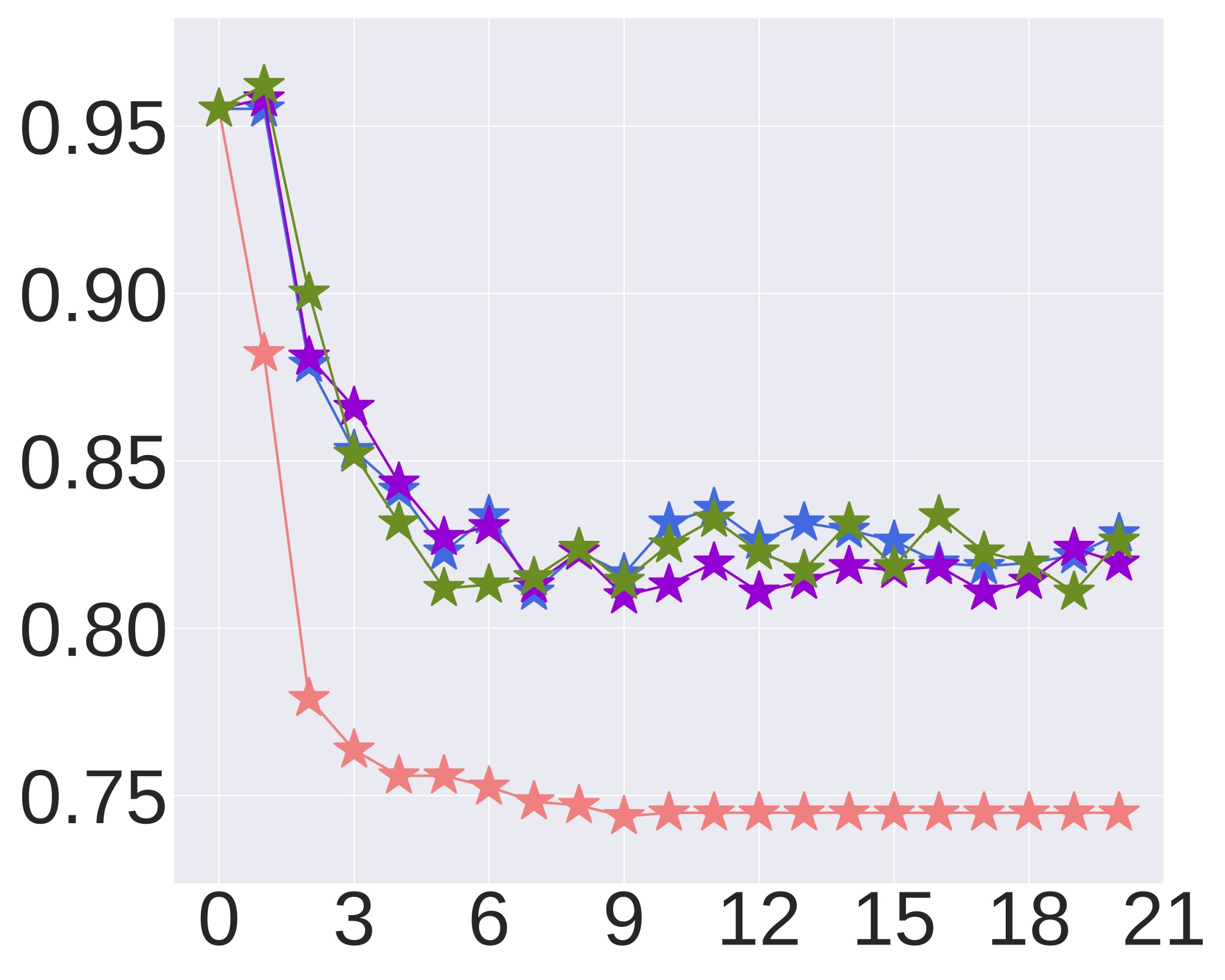
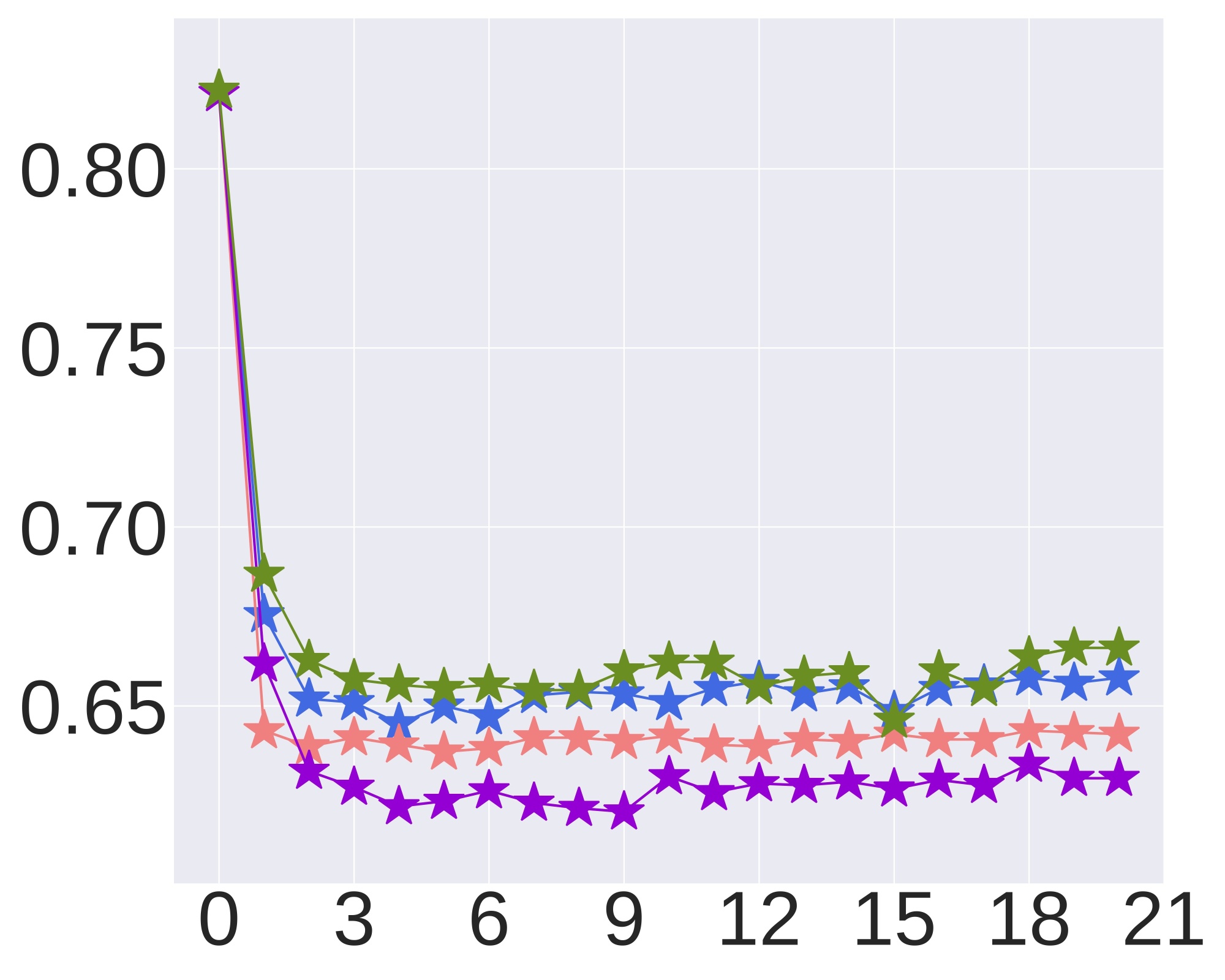
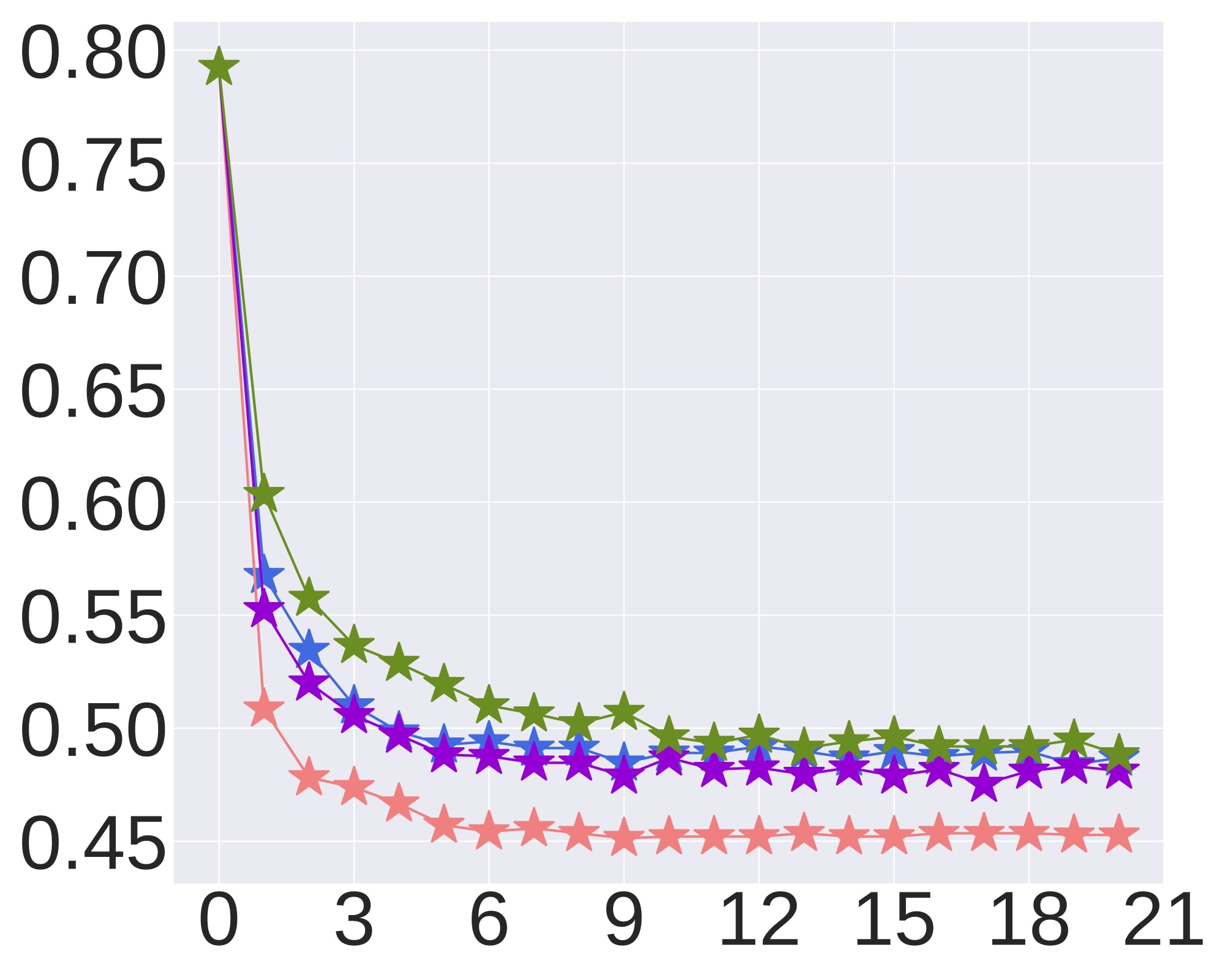
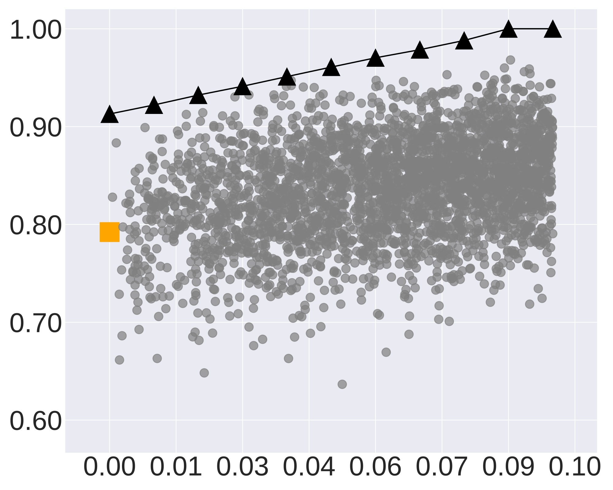
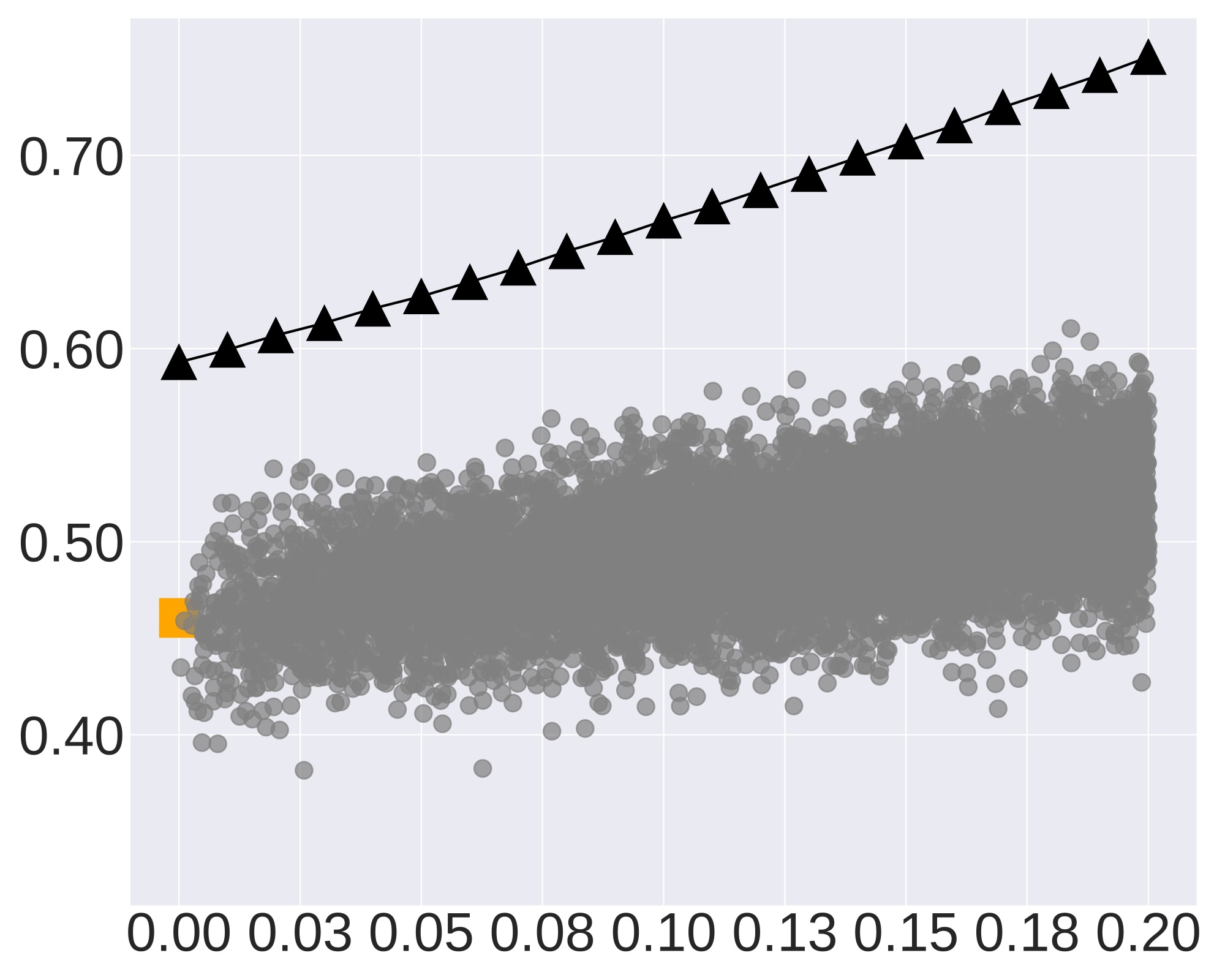
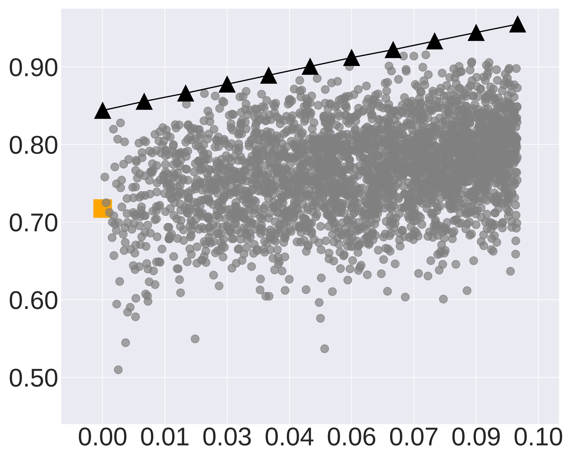
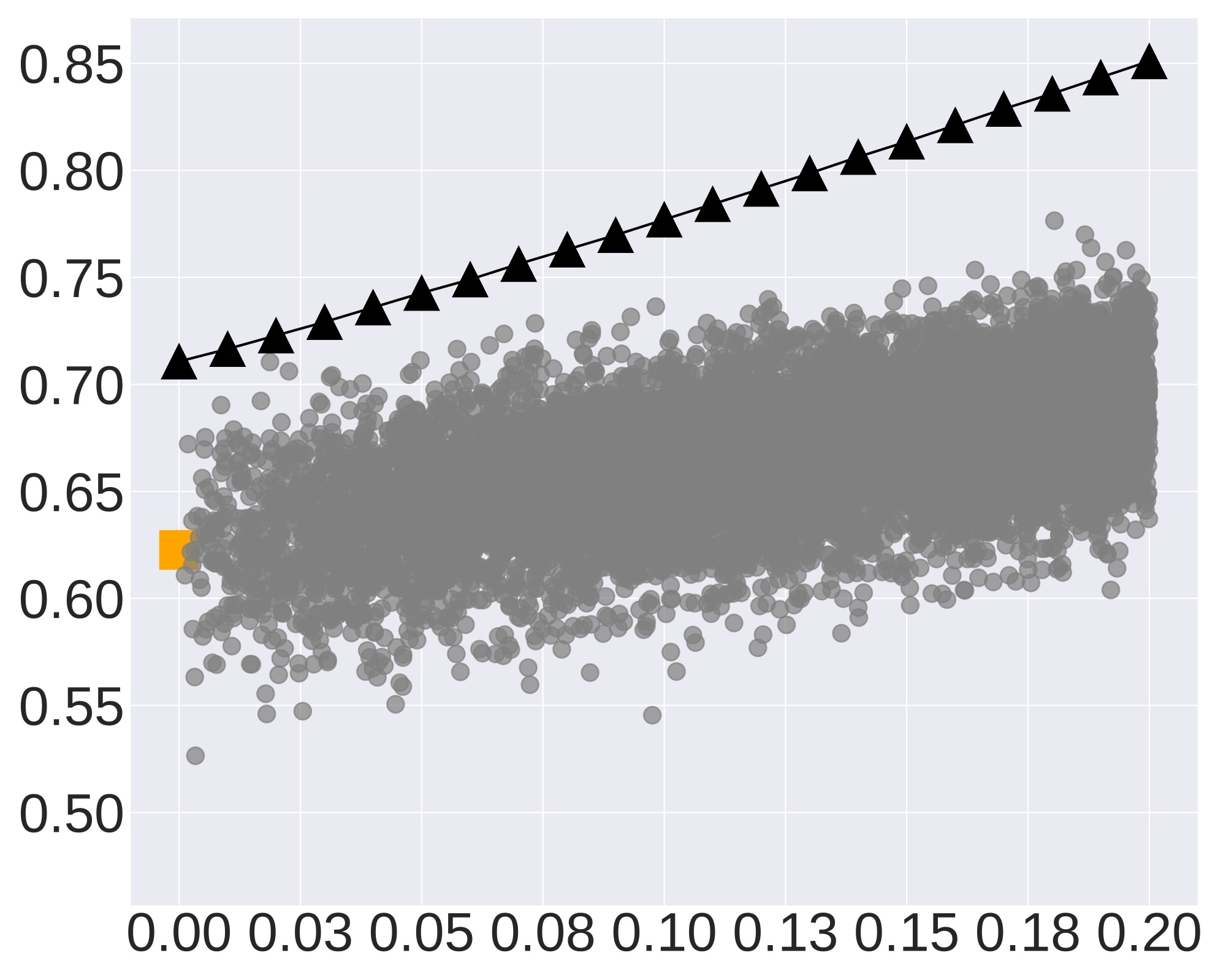
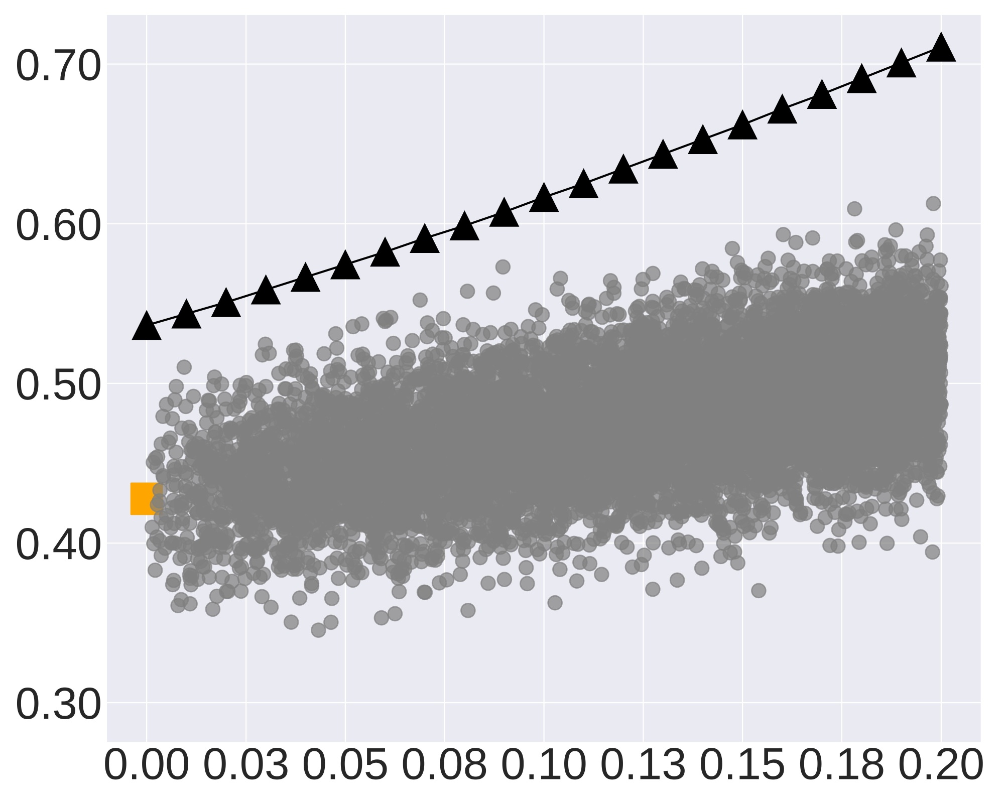
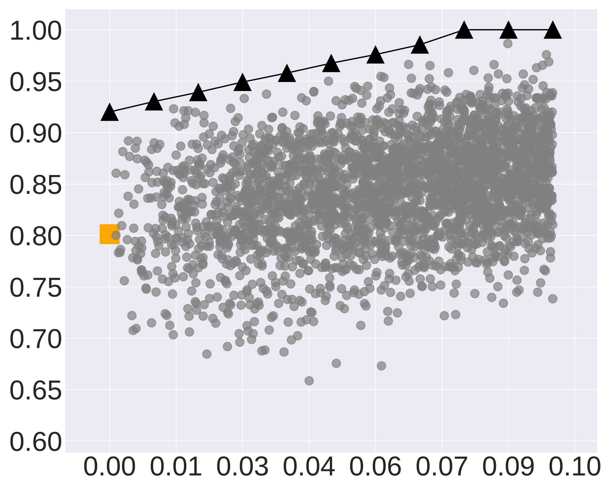
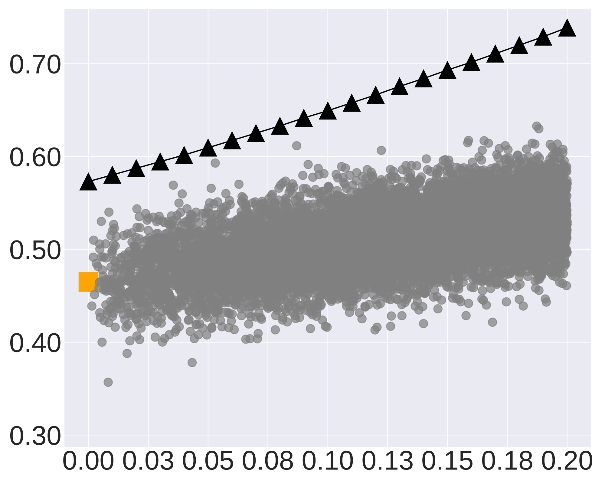
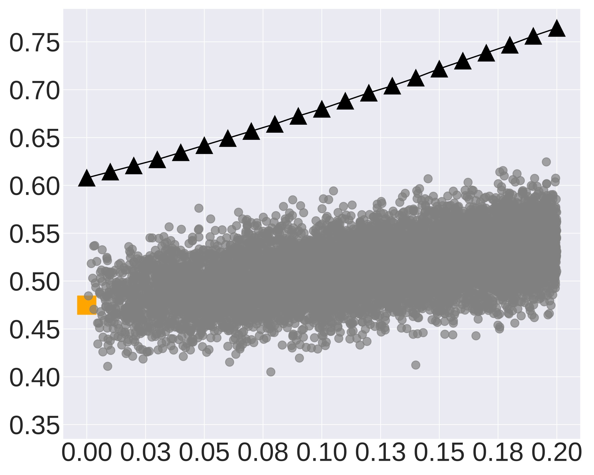
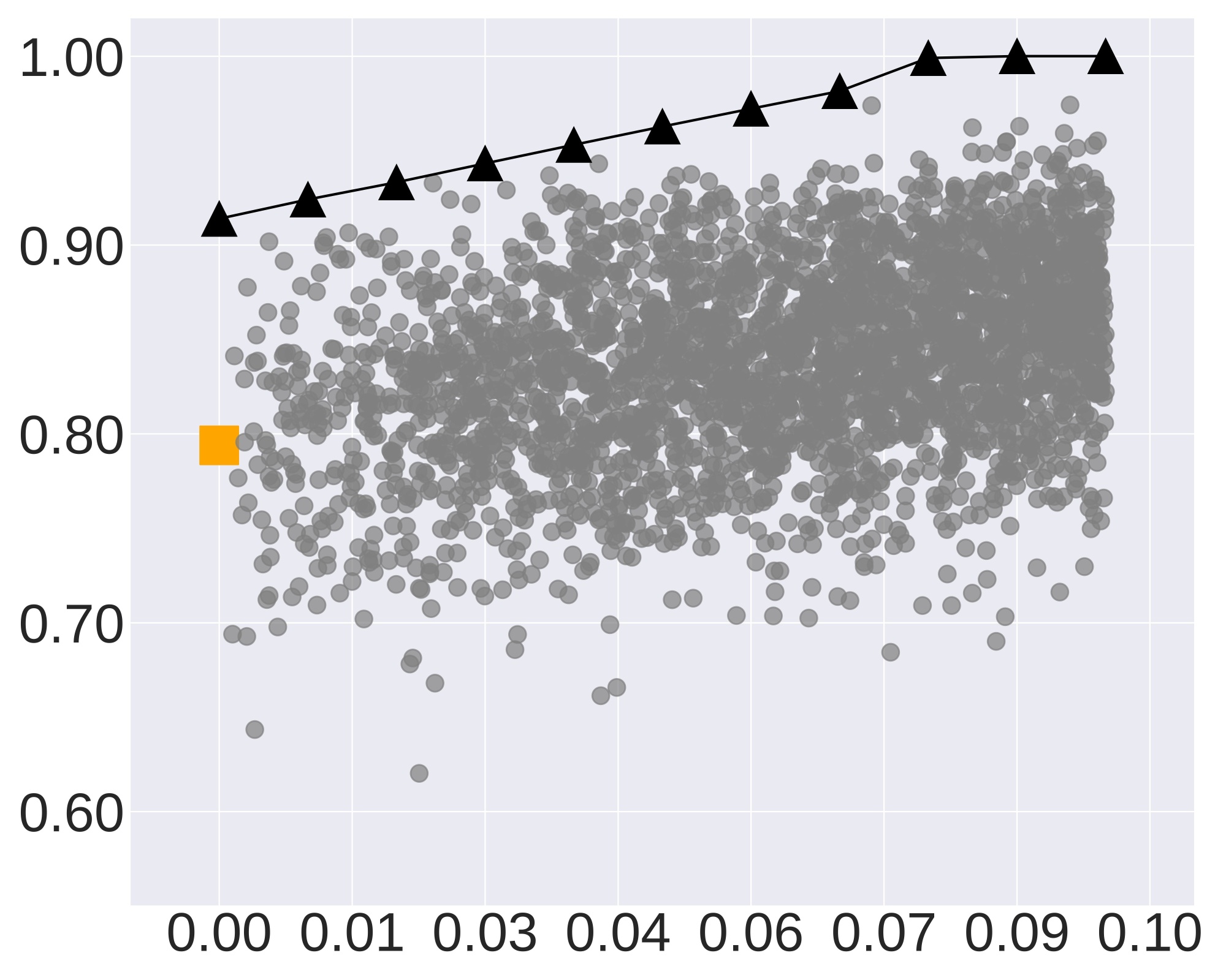
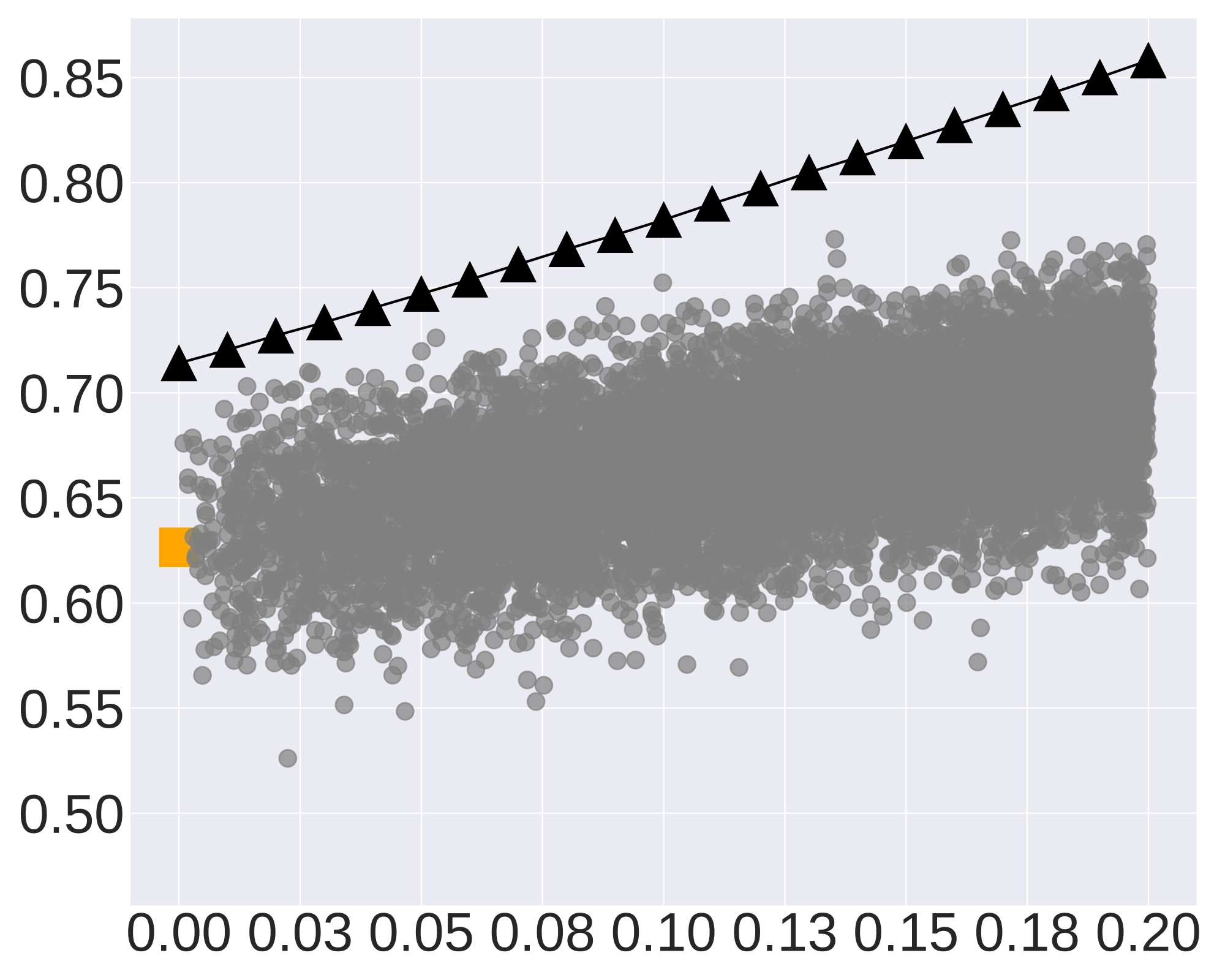
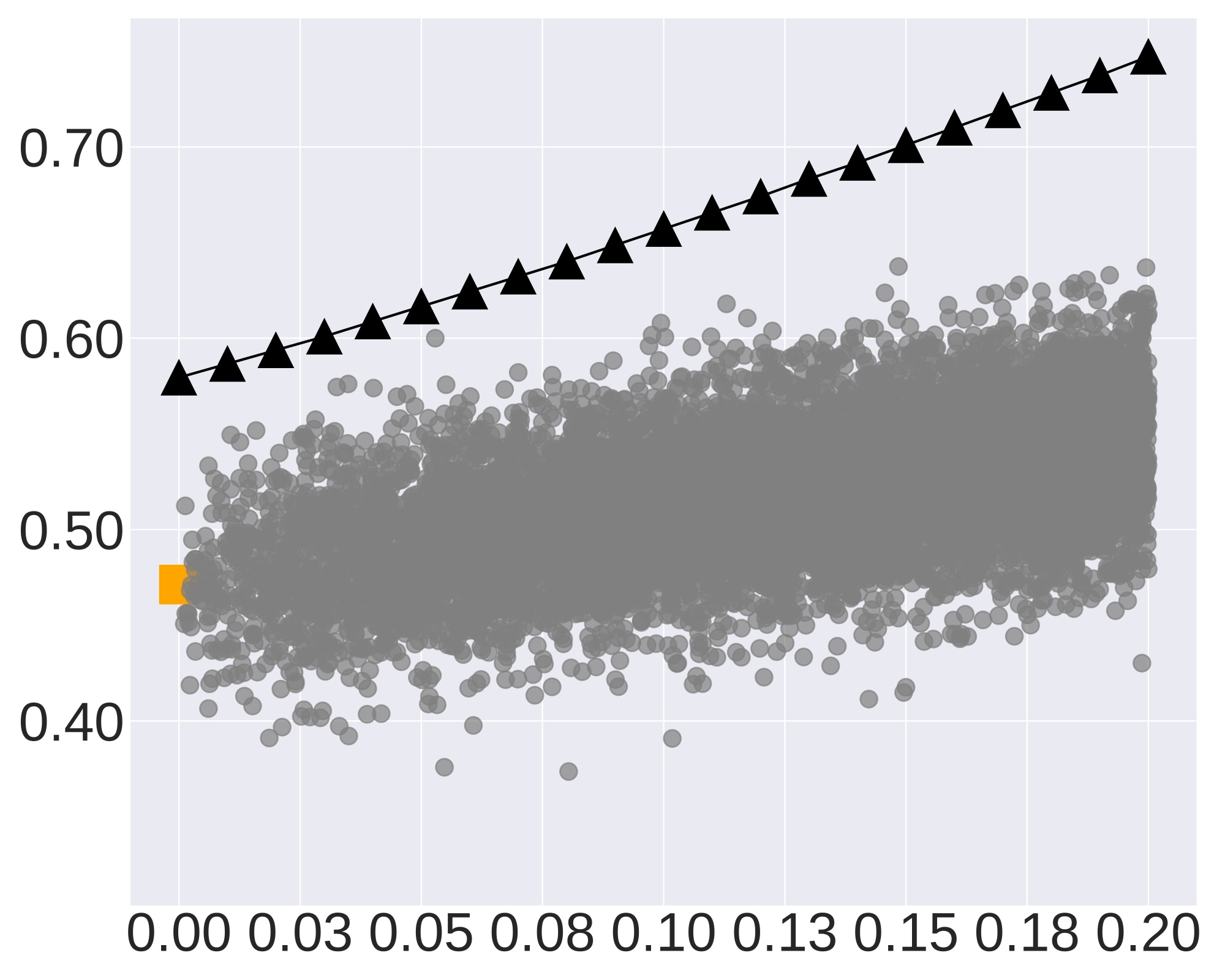
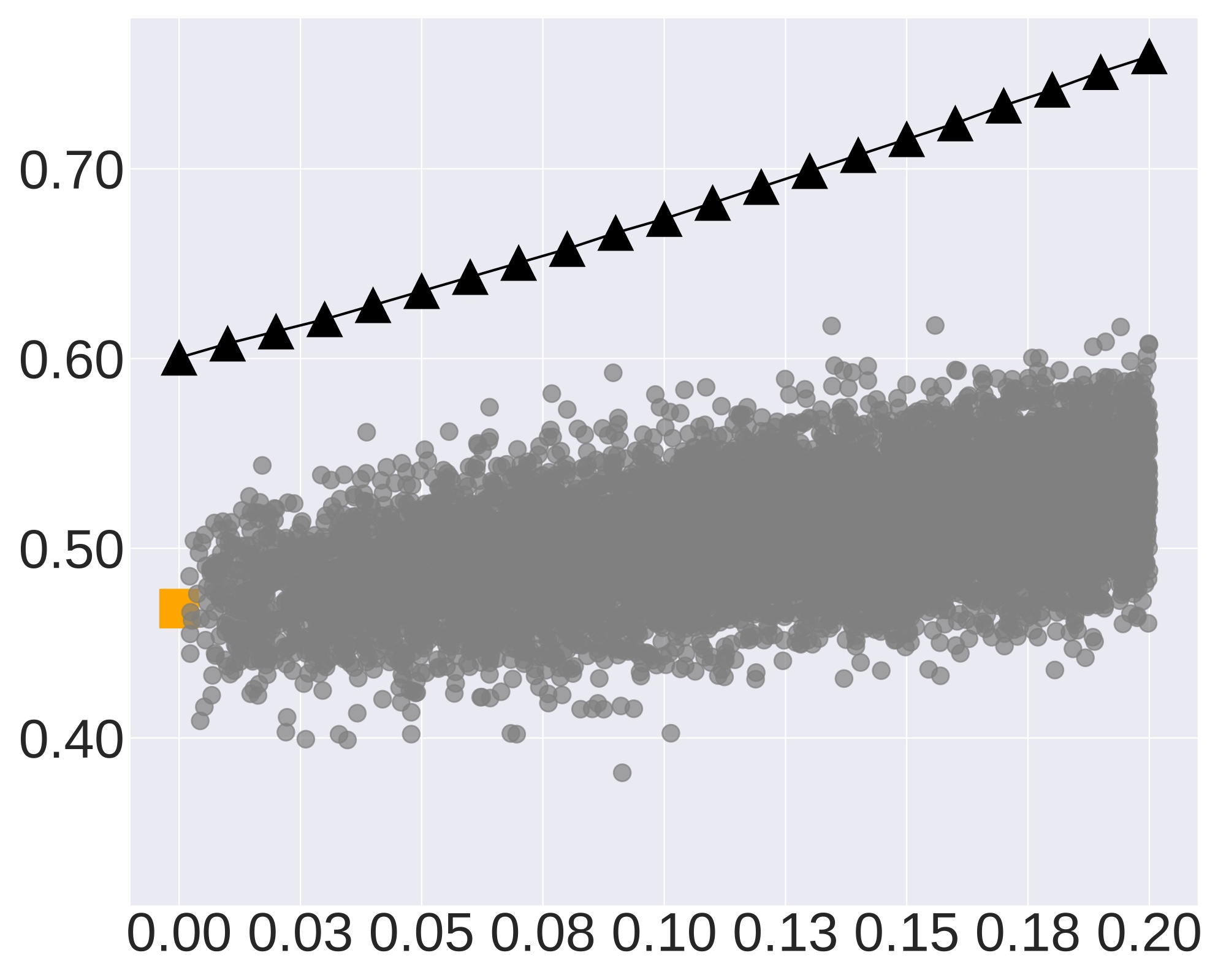
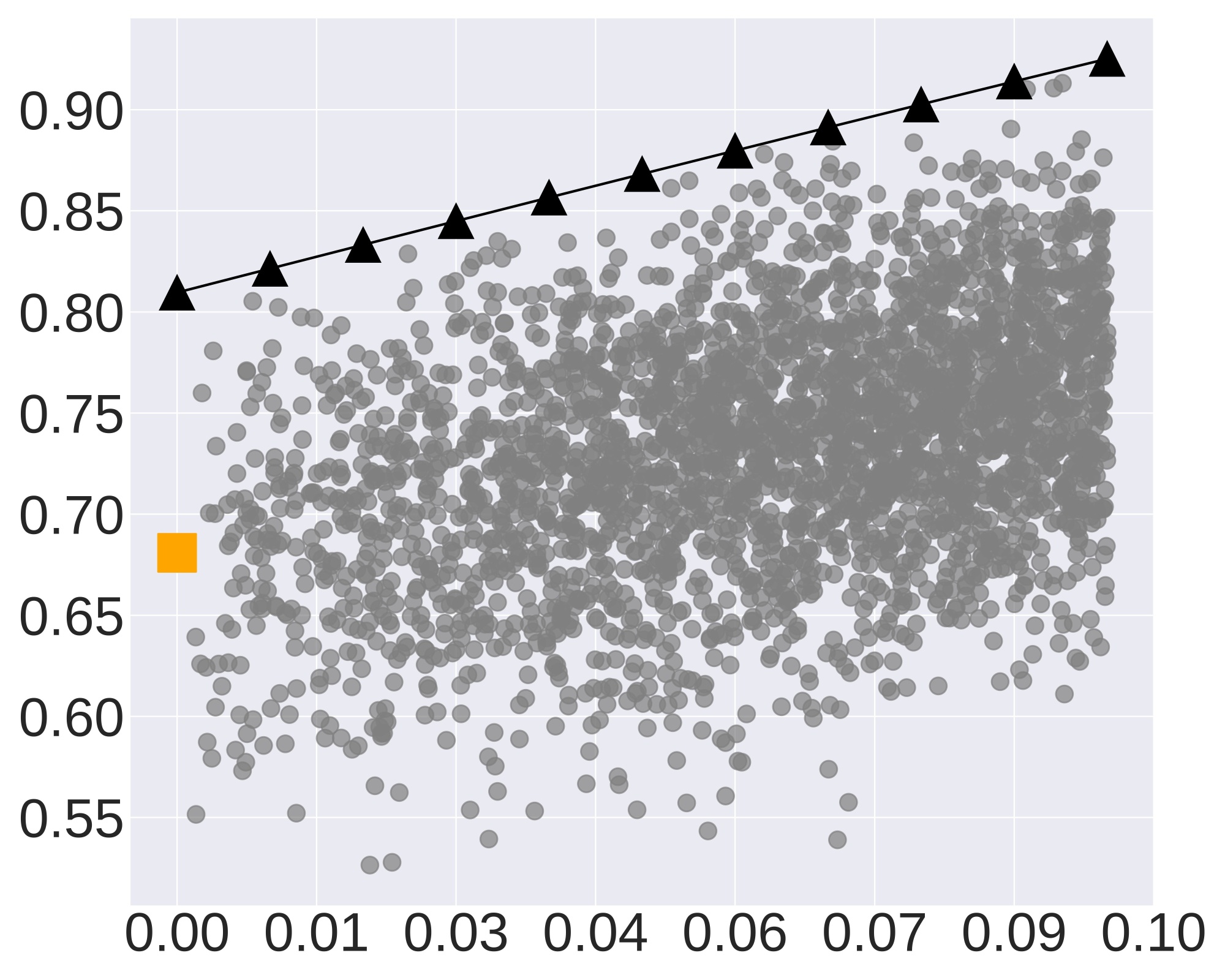
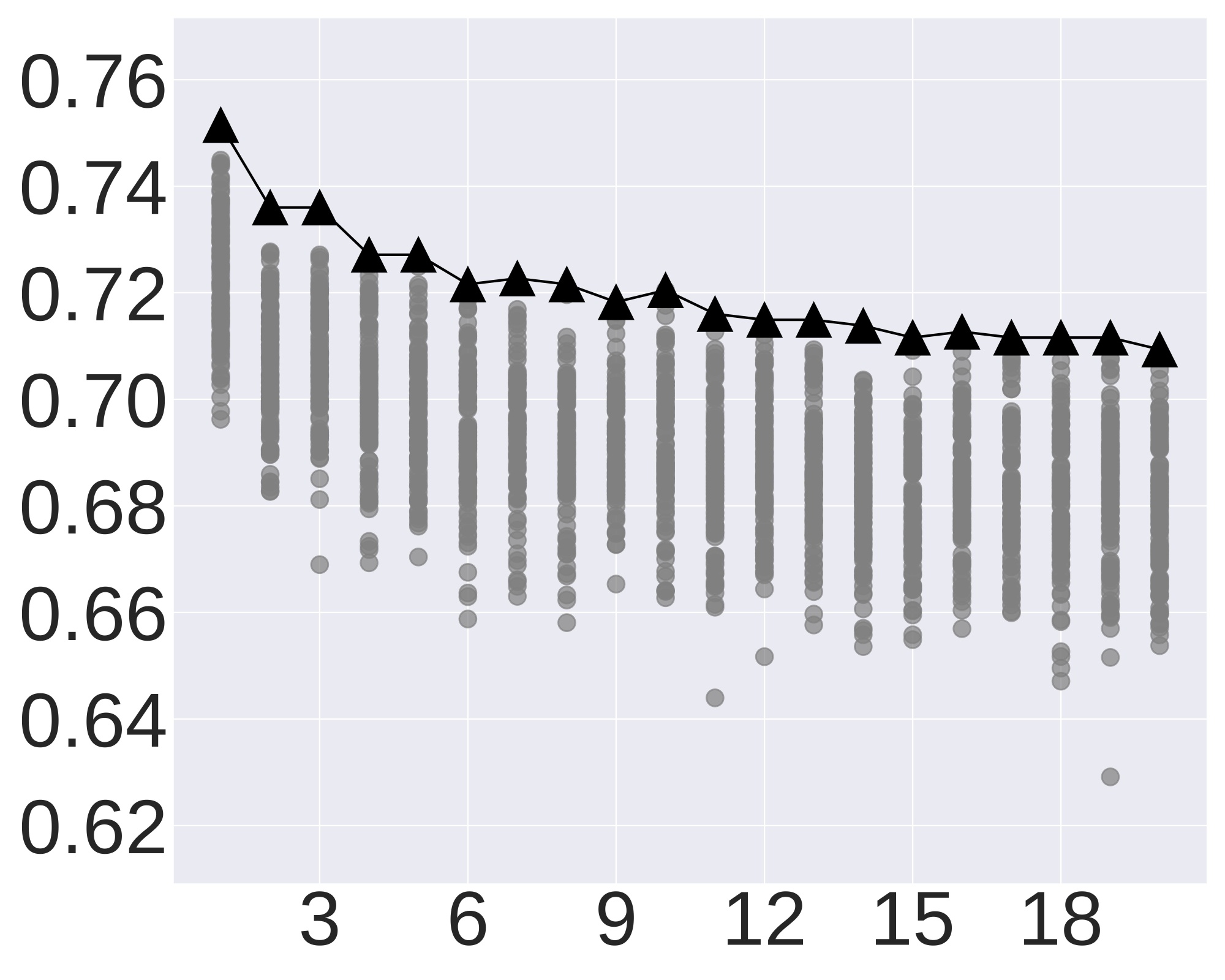
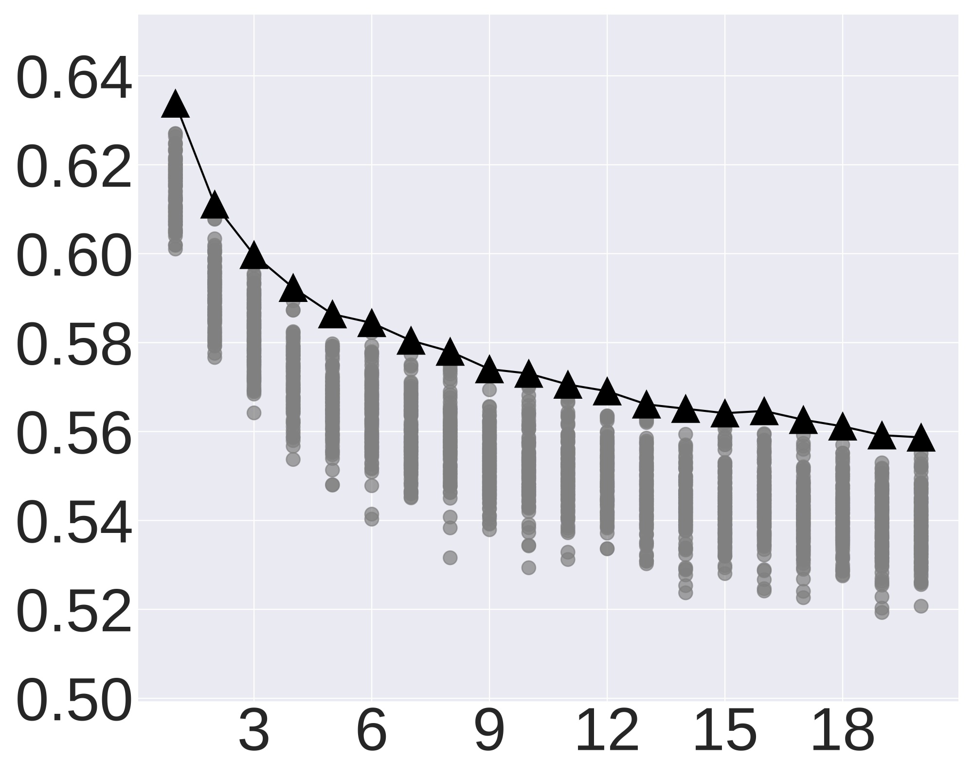
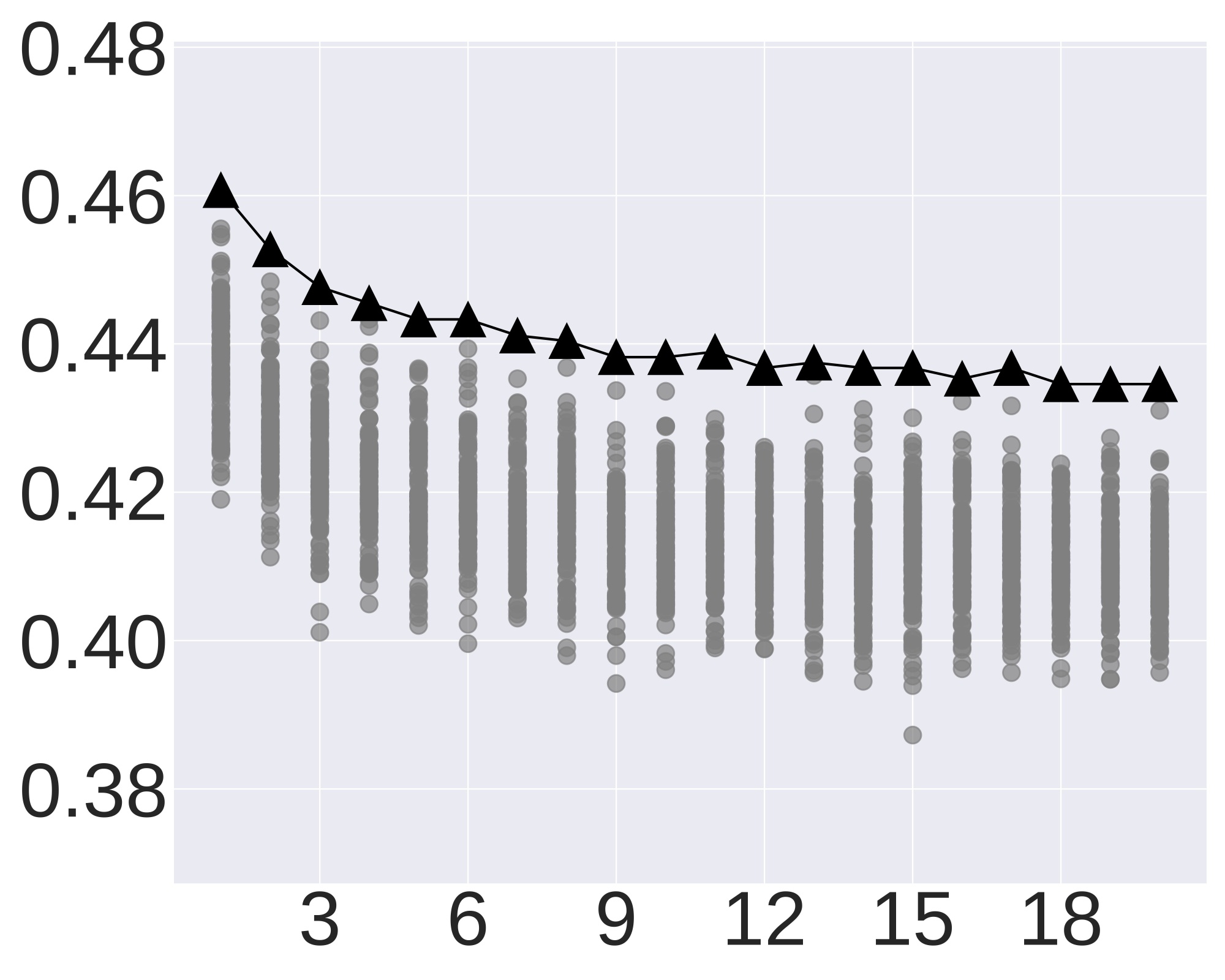
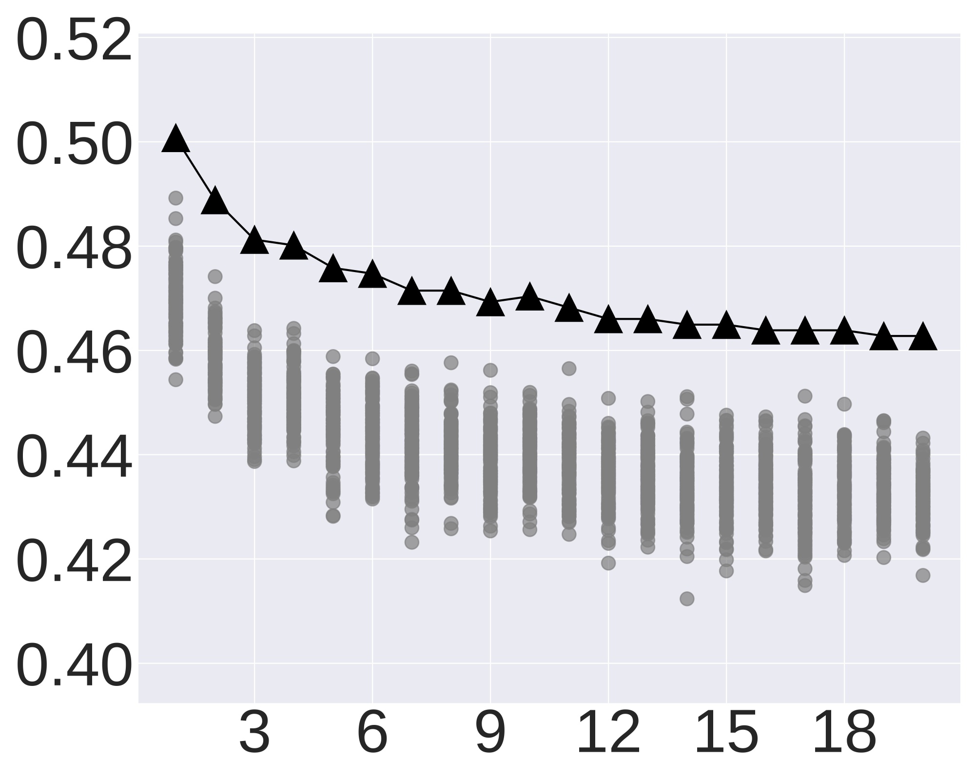
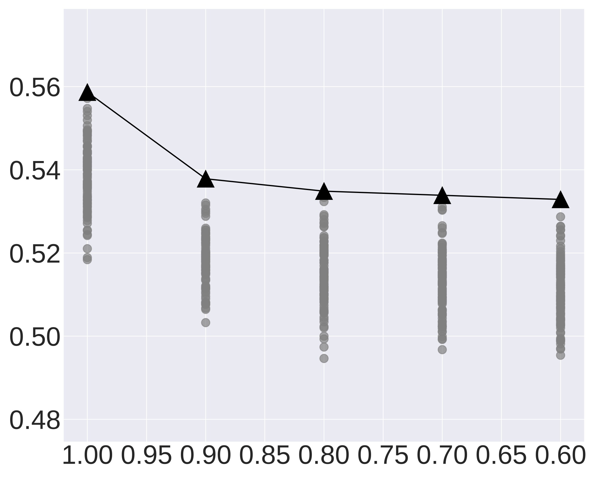
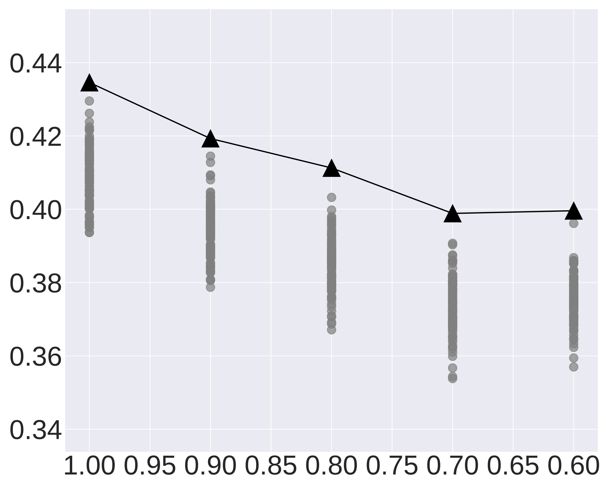
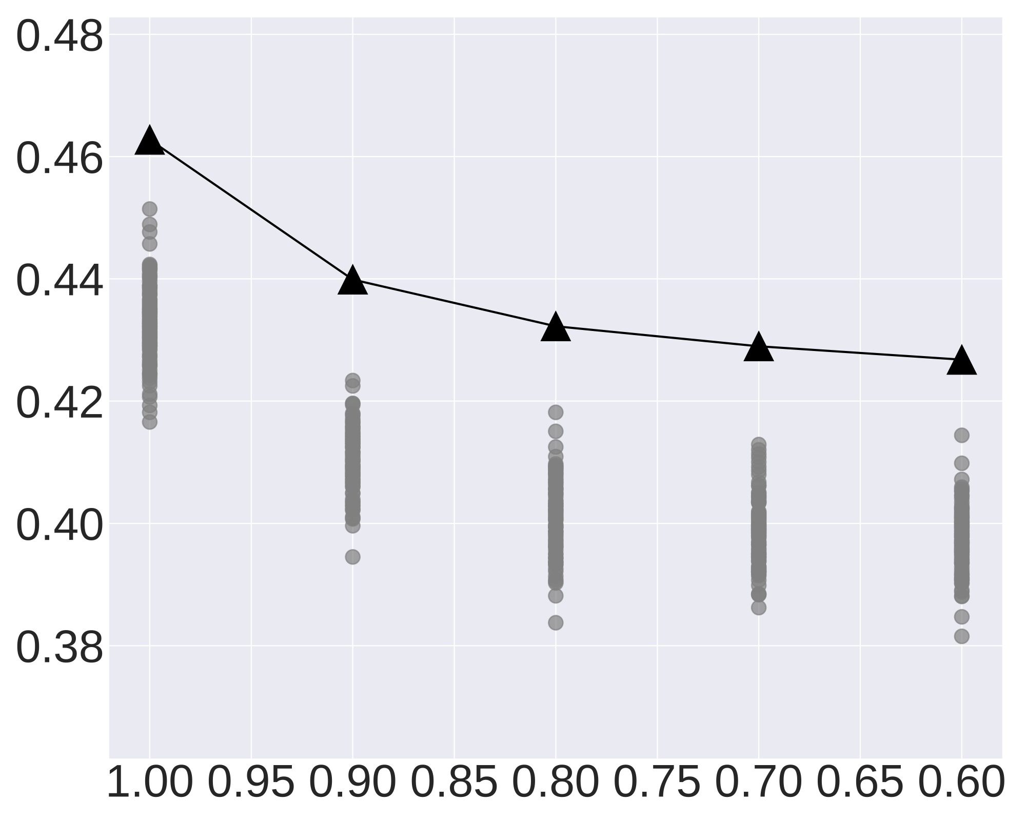
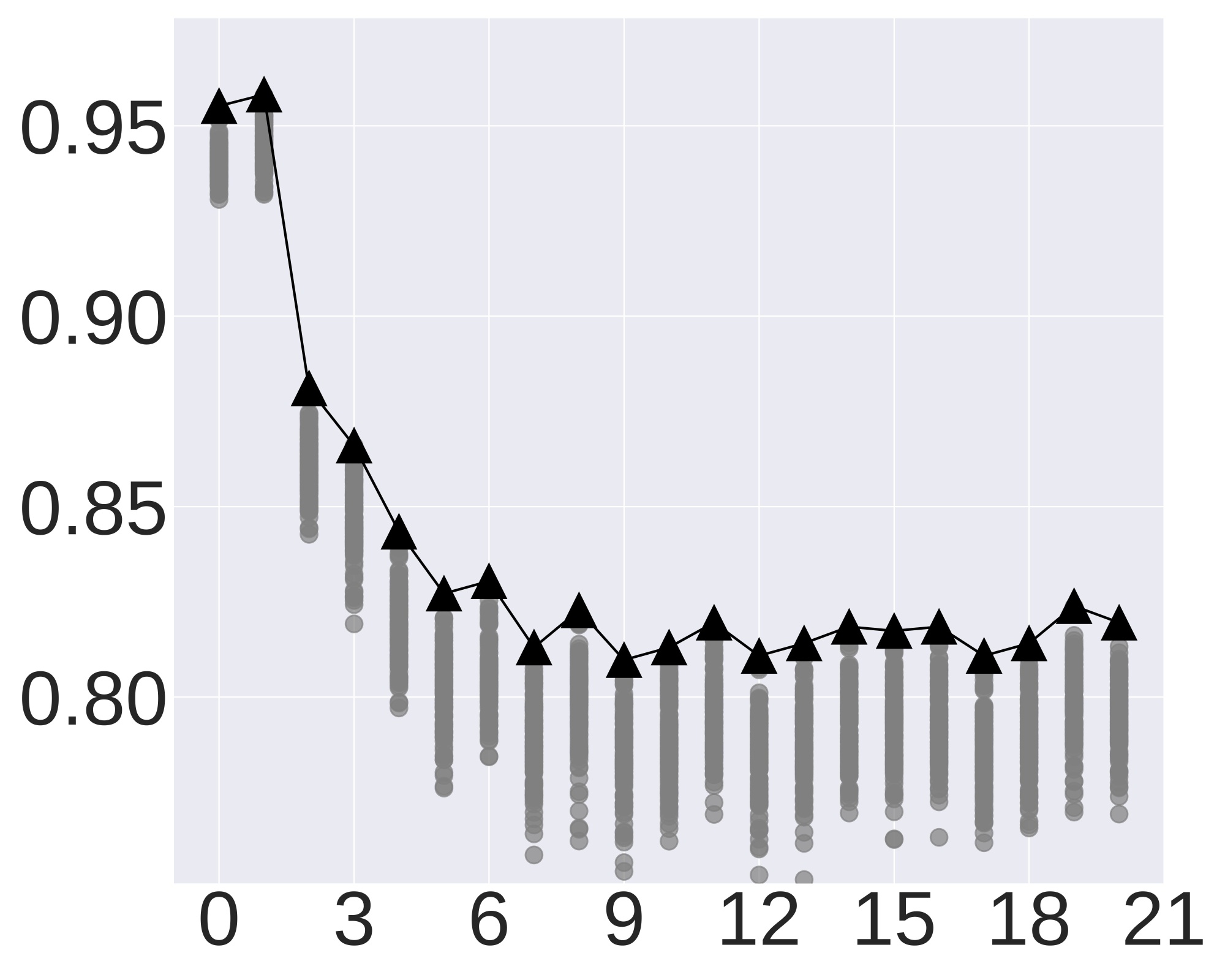
Figure 3: Conformal generation risk α^ragsubscript^𝛼rag\hat{\alpha}_{\text{rag}} (black up-pointing triangles) and empirical risk (gray dots) based on retrieval models OpenAI/ada, Biencoder-SFT, BM25 and BAAI/bge (shown in row 1-4, respectively) given different Nragsubscript𝑁ragN_{\text{rag}} (λg=1,λs=1.0formulae-sequencesubscript𝜆𝑔1subscript𝜆𝑠1.0\lambda_{g}=1,\lambda_{s}=1.0). We observe that our conformal generation risk (Proposition 1) is valid and tight; larger Nragsubscript𝑁ragN_{\text{rag}} reduces conformal generation risk α^ragsubscript^𝛼rag\hat{\alpha}_{\text{rag}} (empirically validating Theorem 1).

 AESLC

Refer to caption

   # Retrieved examples Nragsubscript𝑁ragN_{\text{rag}}

Conformal Risk α^ragsubscript^𝛼rag\hat{\alpha}_{\text{rag}}

 CommonGen

Refer to caption

   # Retrieved examples Nragsubscript𝑁ragN_{\text{rag}}

 DART

Refer to caption

   # Retrieved examples Nragsubscript𝑁ragN_{\text{rag}}

 E2E

Refer to caption

   # Retrieved examples Nragsubscript𝑁ragN_{\text{rag}}

Refer to caption

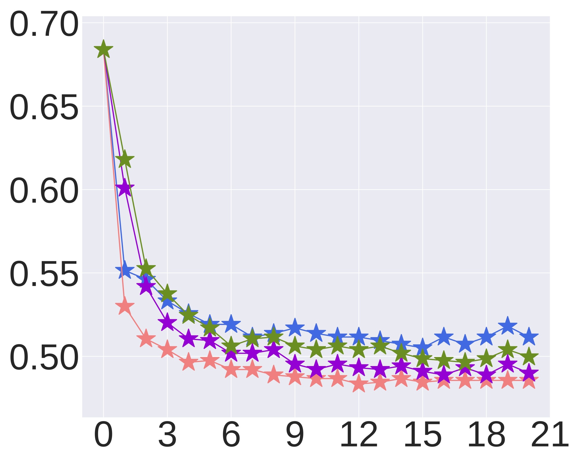
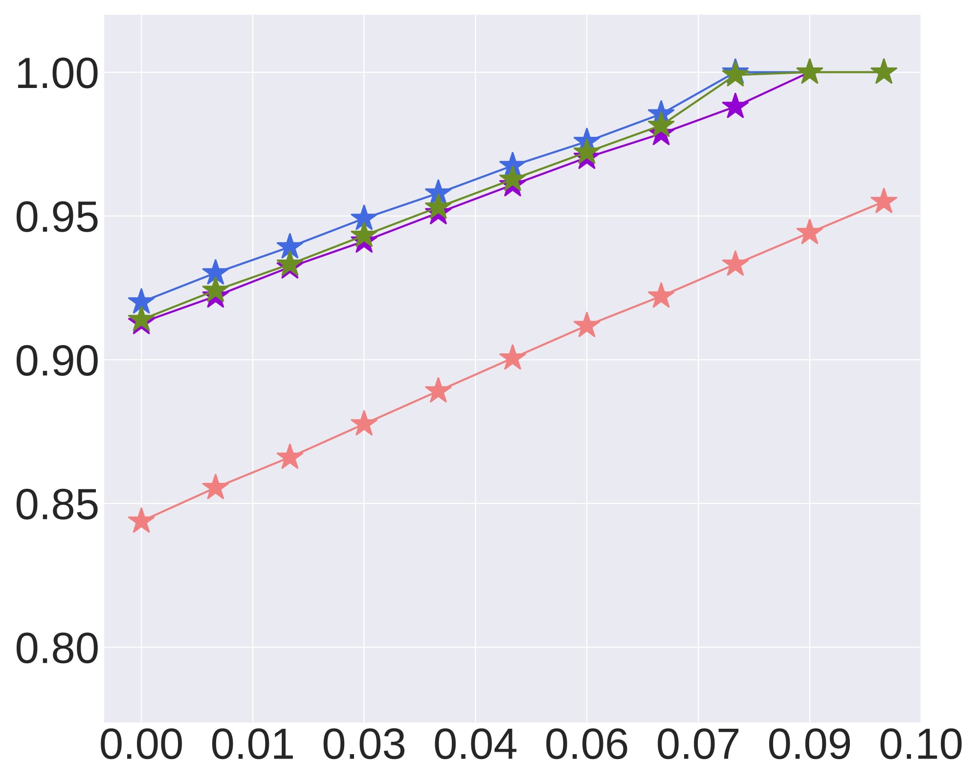
Figure 4: Conformal generation risk α^ragsubscript^𝛼rag\hat{\alpha}_{\text{rag}} with different Nragsubscript𝑁ragN_{\text{rag}} using different retrieval models (λg=1,λs=1.0formulae-sequencesubscript𝜆𝑔1subscript𝜆𝑠1.0\lambda_{g}=1,\lambda_{s}=1.0). We observe that large Nragsubscript𝑁ragN_{\text{rag}} effectively reduces α^ragsubscript^𝛼rag\hat{\alpha}_{\text{rag}} for different models; the trained Biencoder-SFT usually leads to the lowest conformal generation risk.

 AESLC

Refer to caption

Generation risk

 CommonGen

Refer to caption

 DART

Refer to caption

 E2E

Refer to caption

Refer to caption

   Hellinger Distance ρ𝜌\rho

Generation risk

Refer to caption

   Hellinger Distance ρ𝜌\rho

Refer to caption

   Hellinger Distance ρ𝜌\rho

Refer to caption

   Hellinger Distance ρ𝜌\rho

Refer to caption

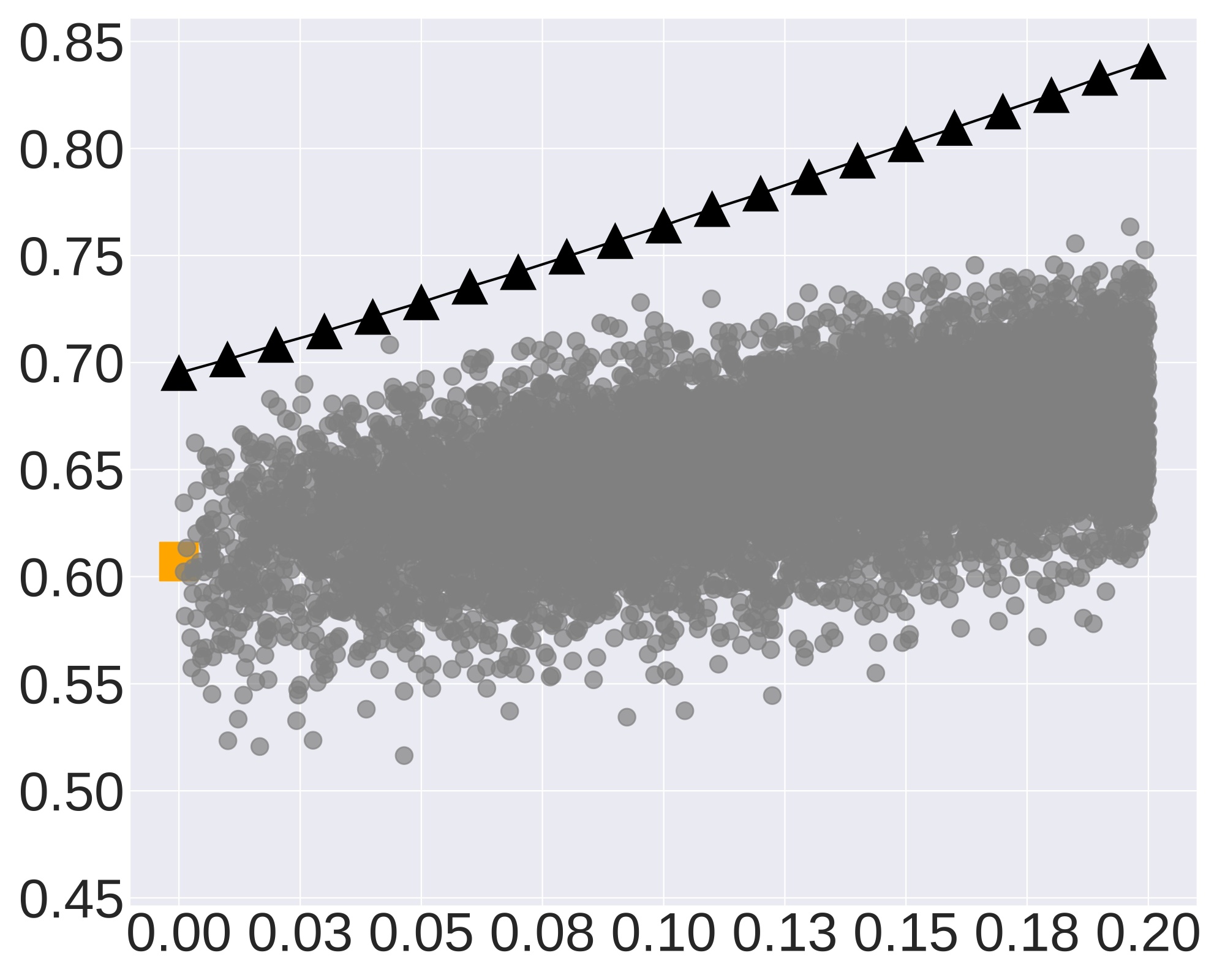
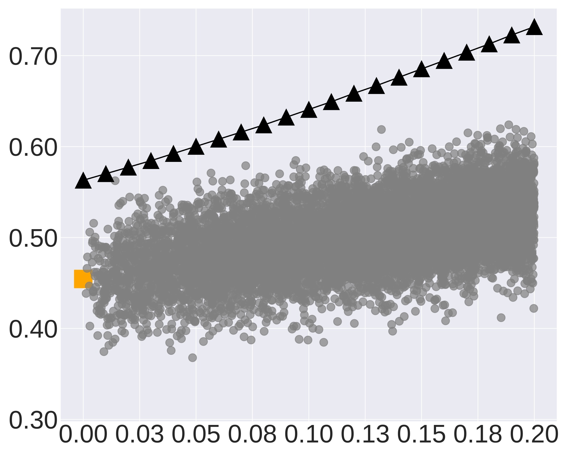
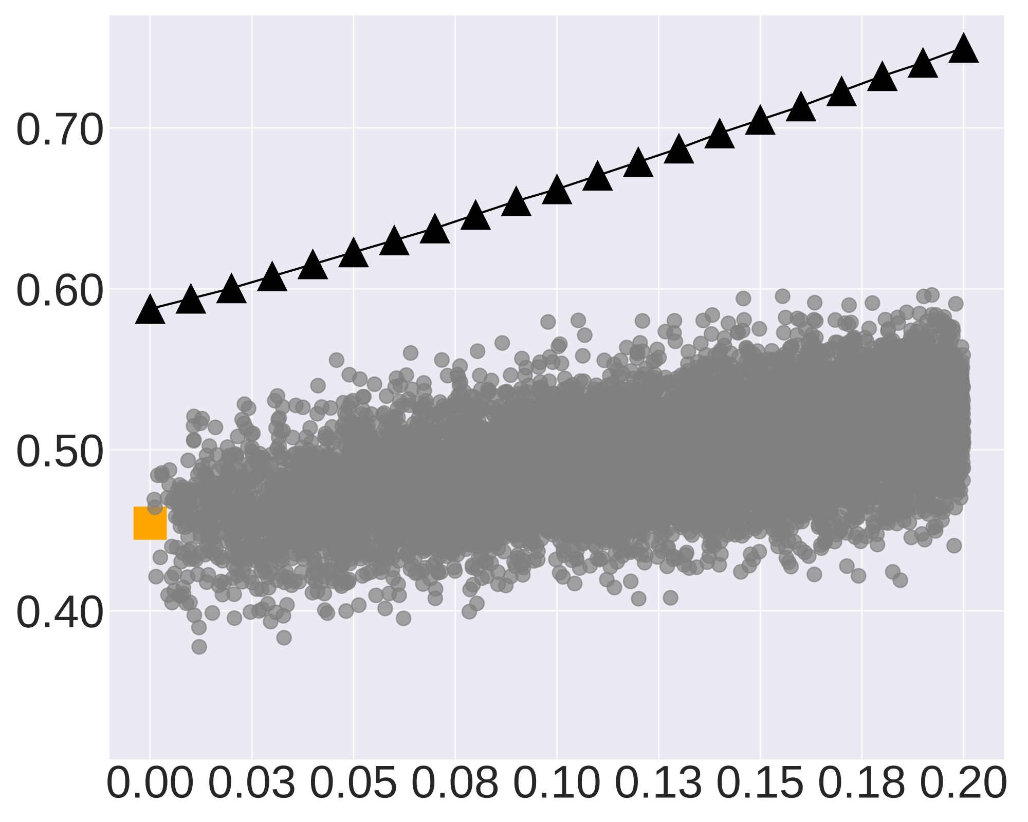
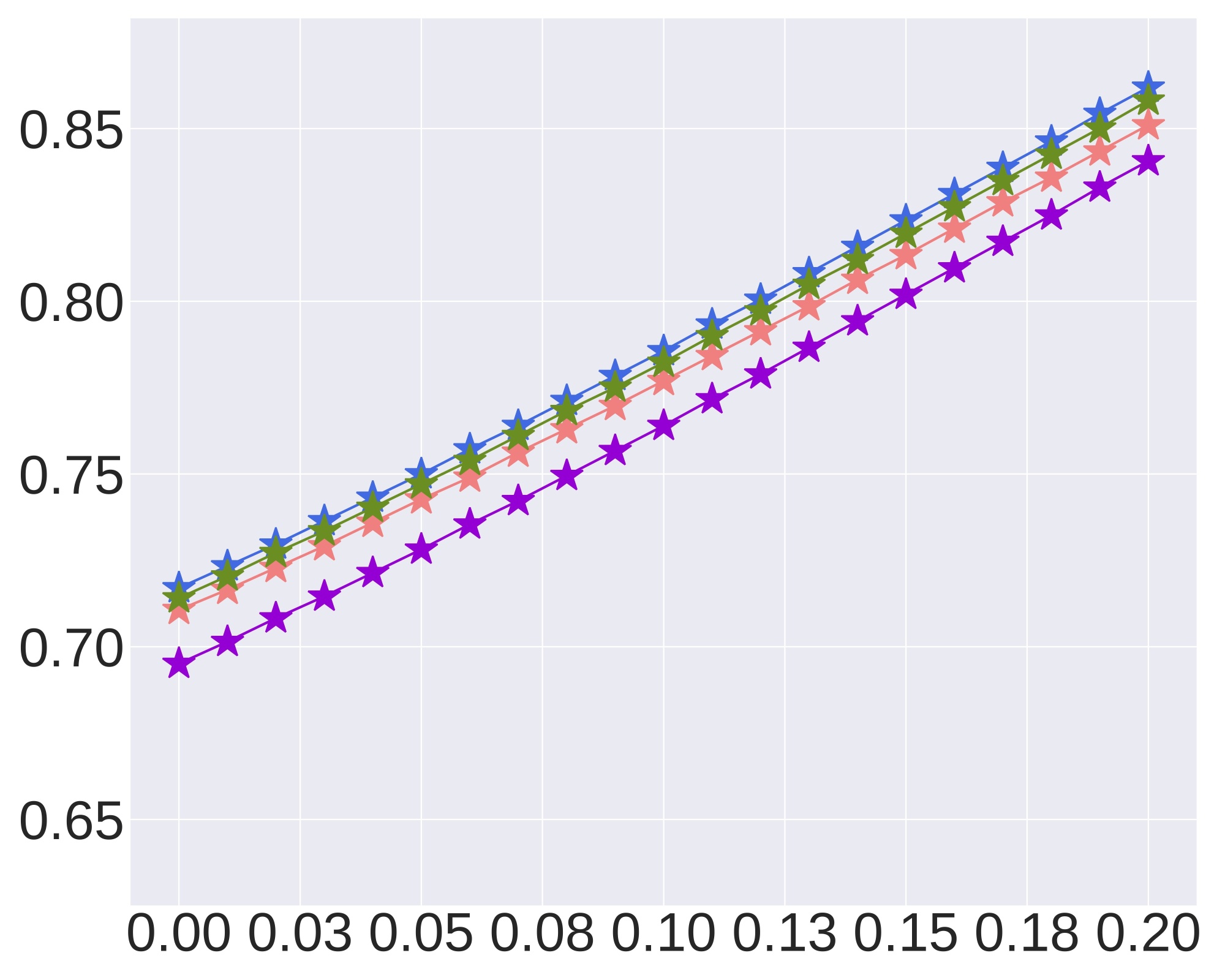
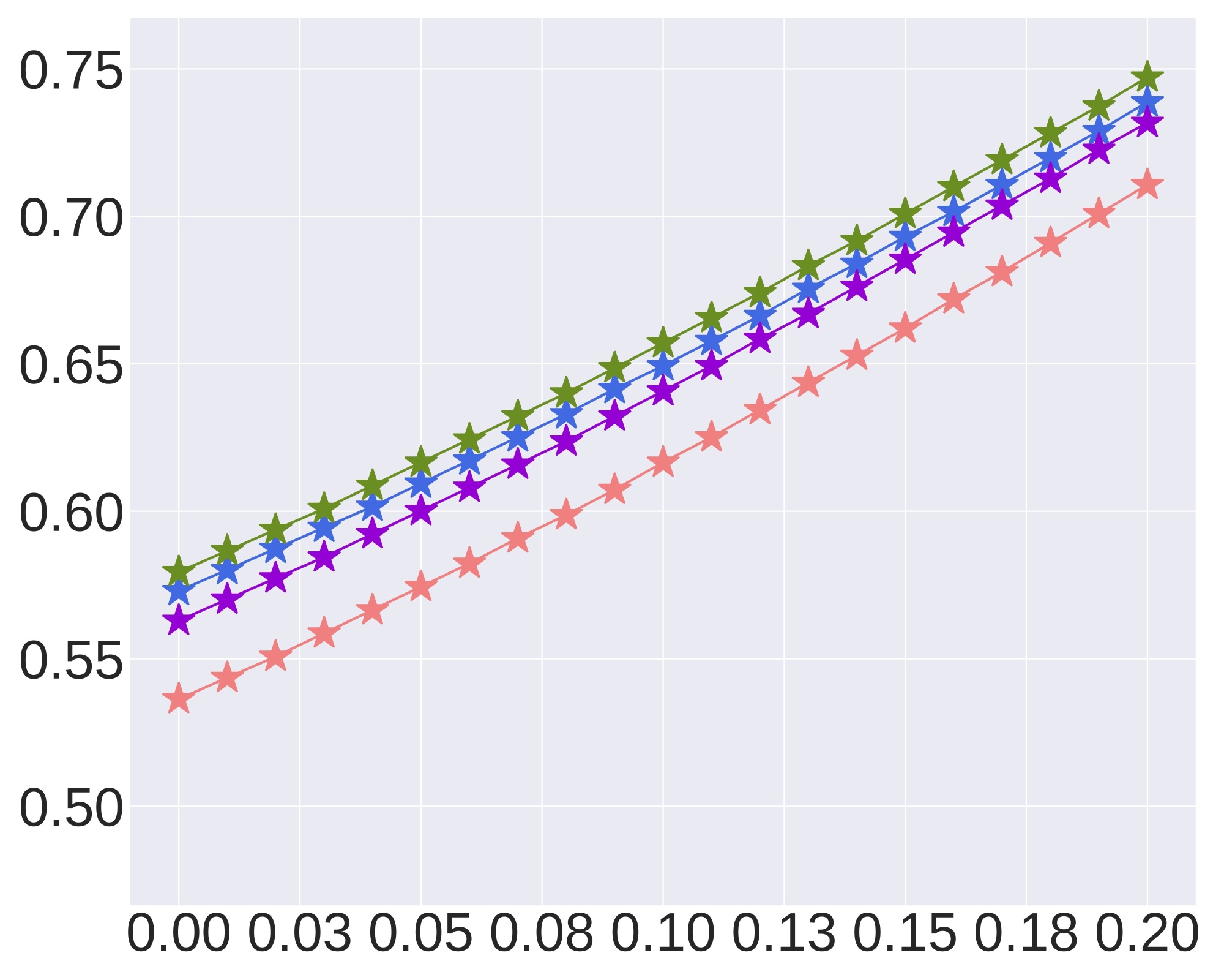
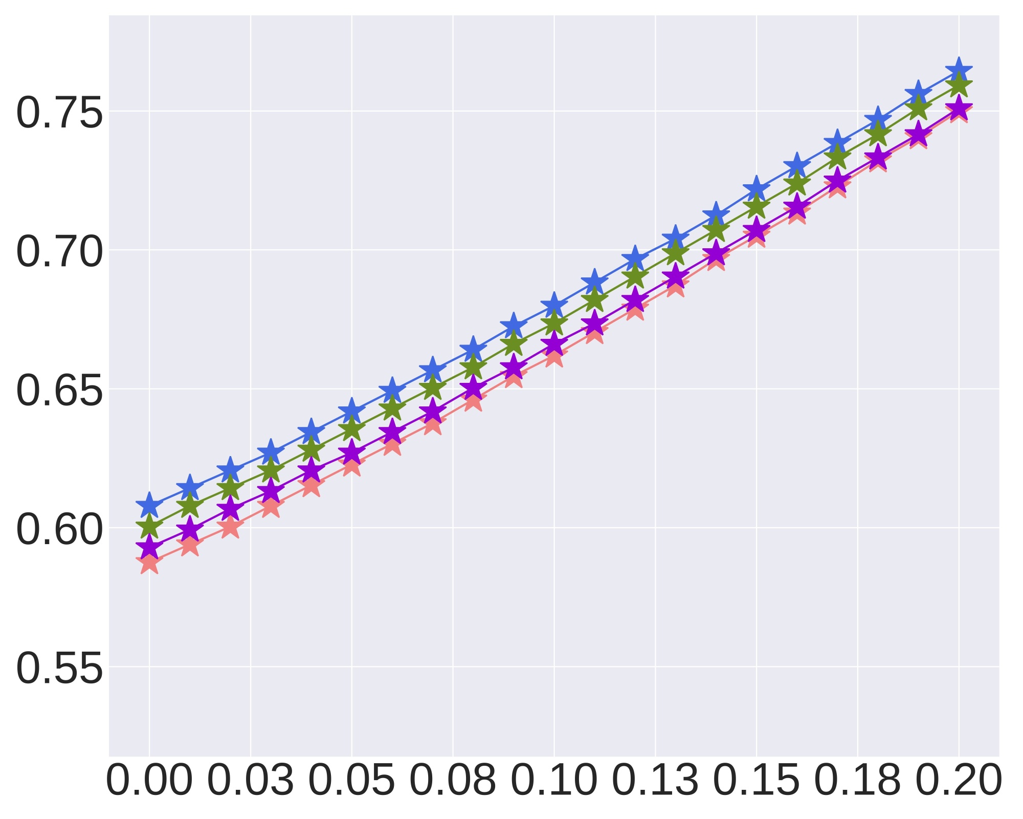
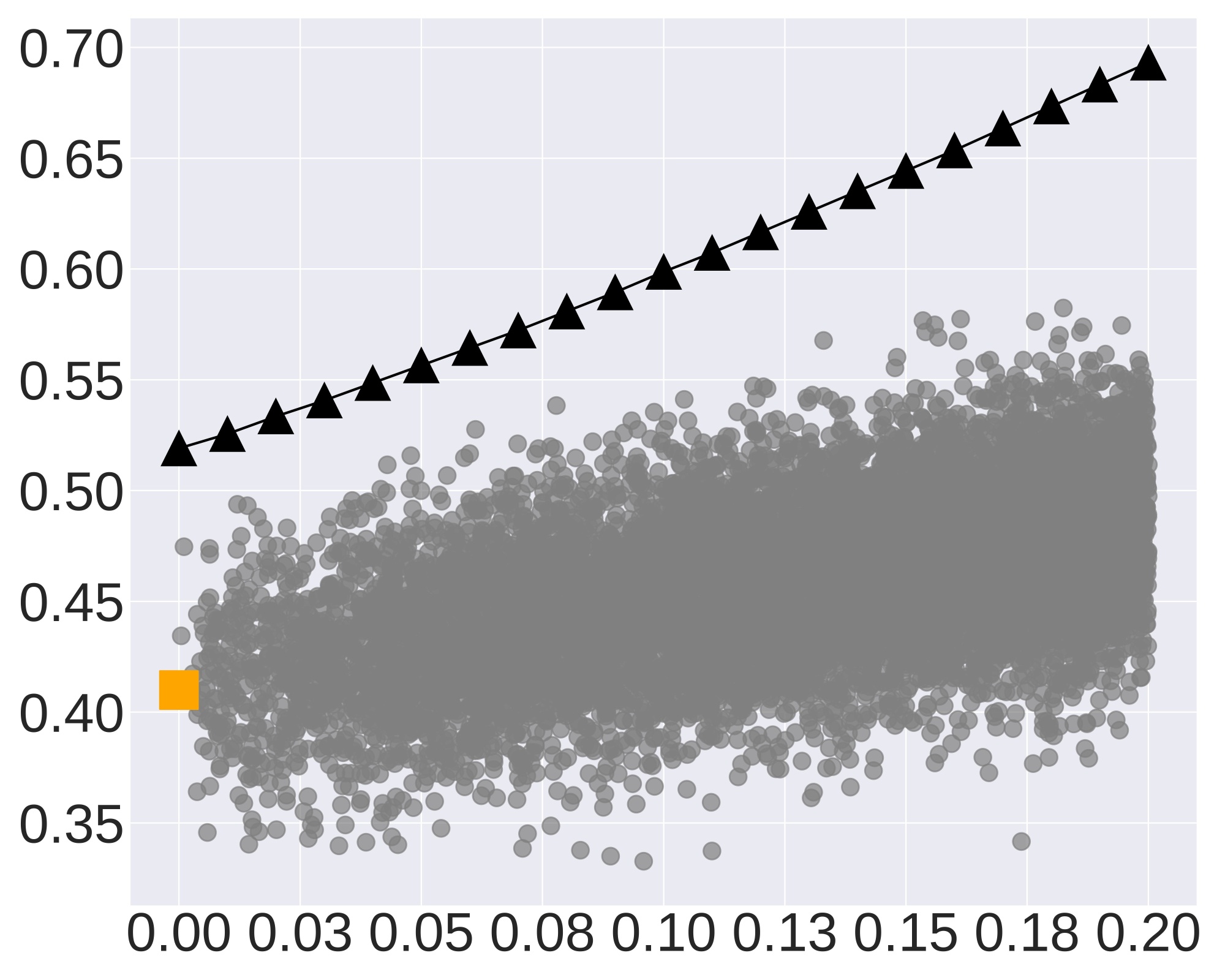
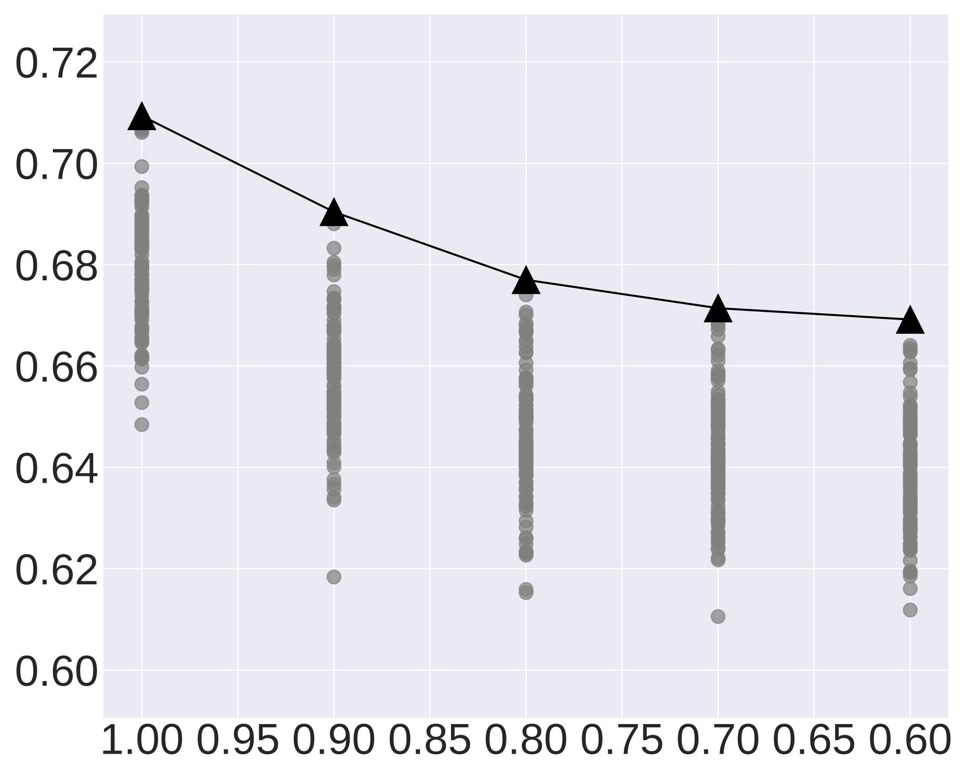
Figure 5: Conformal generation risk α^rag(ρ)subscript^𝛼rag𝜌\hat{\alpha}_{\text{rag}}(\rho) (black up-pointing triangles) and empirical risks (gray dots) based on retrieval model OpenAI/ada and Biencoder-SFT (shown in row 1-2, respectively) under distribution shifts (Nrag=15,λg=1,λs=1.0formulae-sequencesubscript𝑁rag15formulae-sequencesubscript𝜆𝑔1subscript𝜆𝑠1.0N_{\text{rag}}=15,\lambda_{g}=1,\lambda_{s}=1.0). We observe that our distribution-drift conformal generation risk (Theorem 2) is empirically valid and tight.

 AESLC

Refer to caption

 CommonGen

Refer to caption

Refer to caption

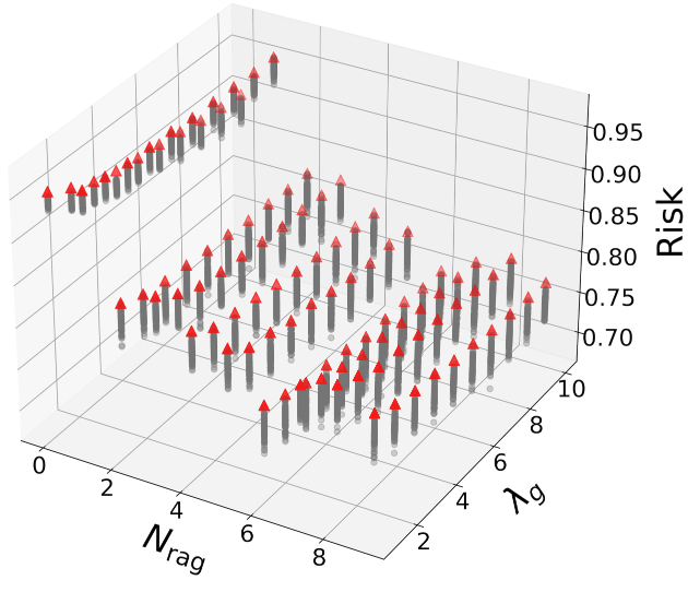
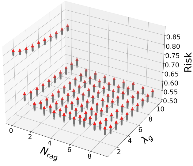
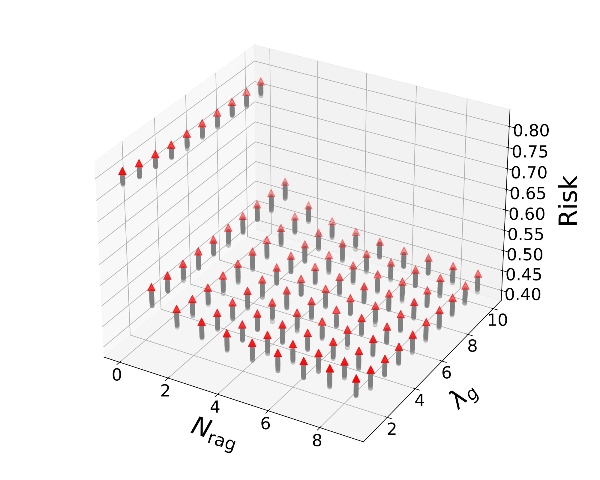
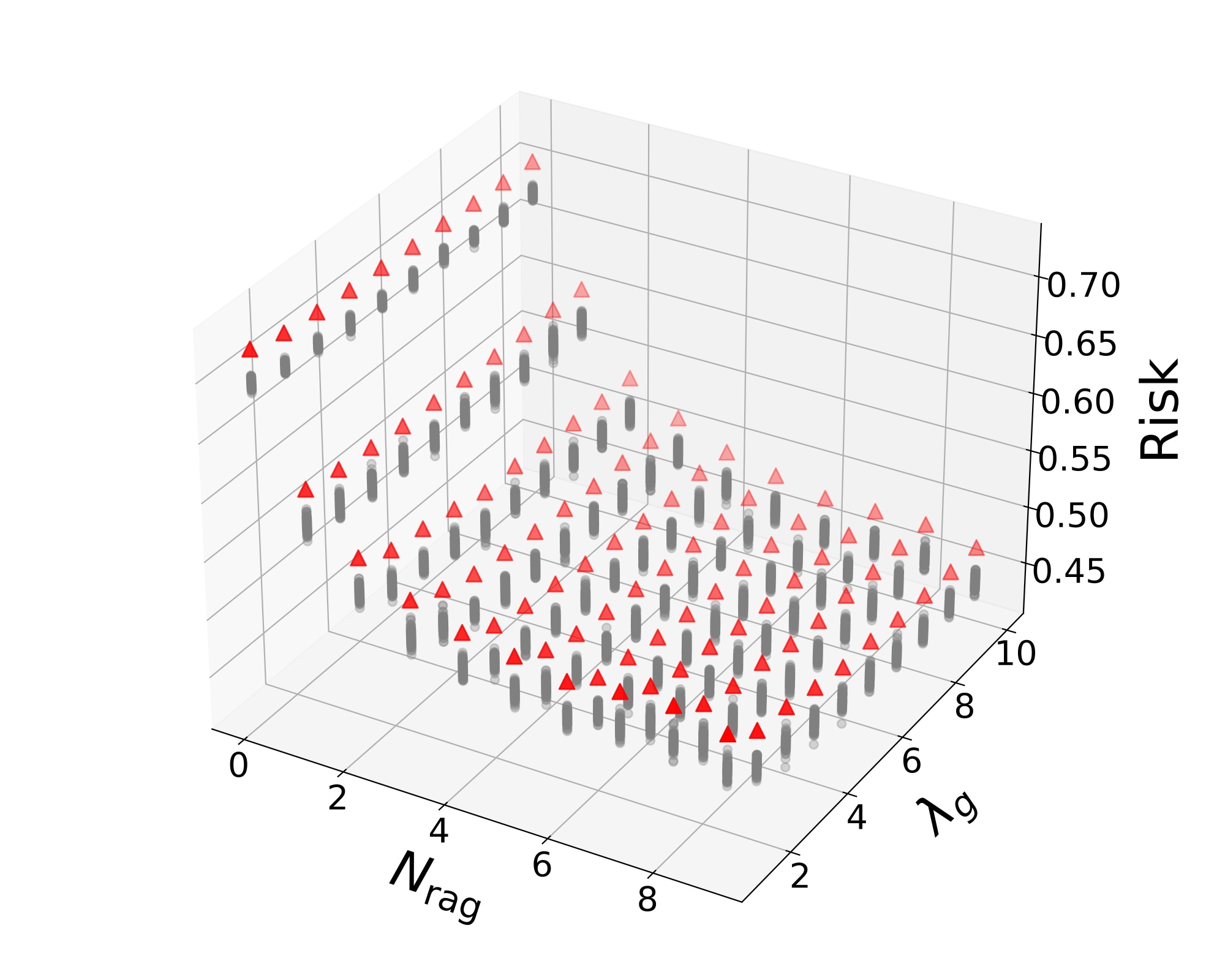
Figure 6: Conformal generation risk α^ragsubscript^𝛼rag\hat{\alpha}_{\text{rag}} and empirical risks with different λgsubscript𝜆𝑔\lambda_{g} and Nragsubscript𝑁ragN_{\text{rag}} for OpenAI/ada.

6 Evaluation

We evaluate C-RAG on four datasets using different retrieval models. We find that (1) our conformal generation risks in Proposition 1 is empirically sound and tight in Section 6.2, (2) RAG reduces the conformal generation risks for different retrieval models, which empirically validates Theorem 1 in Section 6.2, (3) the conformal generation risk under distribution shifts in Theorem 2 is empirically sound and tight for varying distances in Section 6.3, (4) multi-dimensional RAG configurations maintain sound and tight conformal generation risks in Section 6.4, and (5) C-RAG computes valid configurations with empirical risks always below the desired risk level in Section 6.5.

Codes are publicly available at https://github.com/kangmintong/C-RAG.

6.1 Evaluation setup

Datasets & knowledge base

We evaluate C-RAG on four widely used NLP datasets, including AESLC (Zhang & Tetreault, 2019), CommonGen (Lin et al., 2019), DART (Nan et al., 2020), and E2E (Novikova et al., 2017). Following (Wang et al., 2023b; Cheng et al., 2023), we construct the knowledge base as a collection of 30 public datasets from 9 distinct categories with over 6 million documents.

Retrieval models

We consider four retrieval models: (1) BM25 (Robertson et al., 2009) with token-level matching scores, (2) BAAI/bge (Zhang et al., 2023a) as SOTA embedding model in MTEB benchmark (Muennighoff et al., 2022), (3) OpenAI/ada as SOTA close source text embedding model, and (4) Biencoder-SFT (Wang et al., 2023b) as a biencoder retriever trained with in-domain data samples.

RAG Generation protocol

We use our generation protocol (Algorithm 1 in Section C.1) controlled by the number of retrieved examples Nragsubscript𝑁ragN_{\text{rag}}, generation set size λgsubscript𝜆𝑔\lambda_{g}, and diversity threshold λssubscript𝜆𝑠\lambda_{s}. We use Llama-7b for inference and perform conformal calibration on validation sets with uncertainty δ=0.1𝛿0.1\delta=0.1. We use 1ROUGE-L1ROUGE-L1-\text{ROUGE-L} as the risk function. See Section J.1 for more details of evaluation setup.

 AESLC
Refer to caption

 CommonGen

Refer to caption

Refer to caption

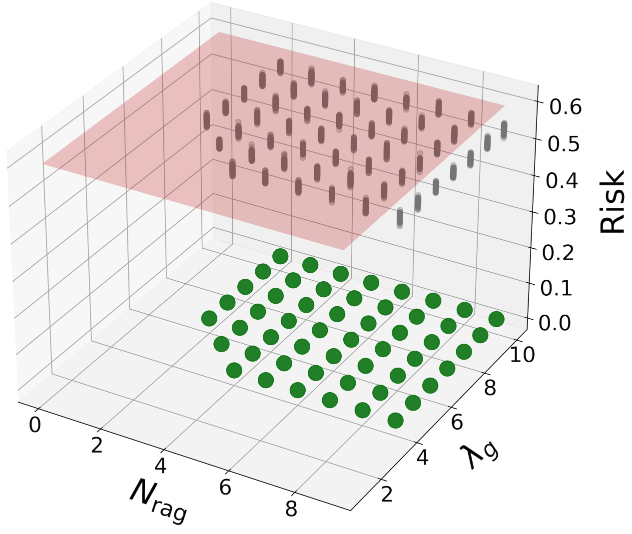
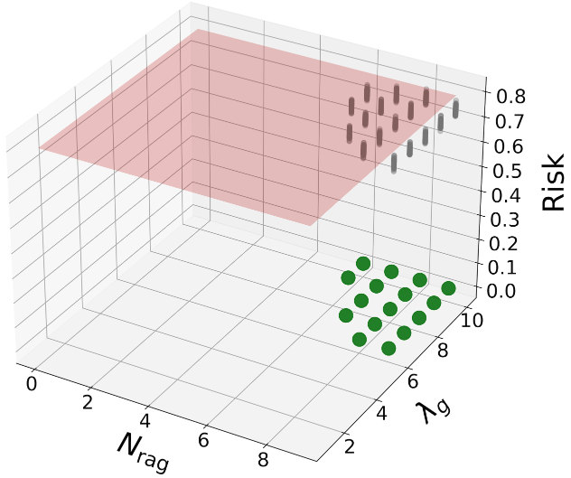
Figure 7: Valid configurations Λ^αsubscript^Λ𝛼\hat{\Lambda}_{\alpha} given a desired risk level α𝛼\alpha and the empirical risks with different λgsubscript𝜆𝑔\lambda_{g} and Nragsubscript𝑁ragN_{\text{rag}} for OpenAI/ada.

6.2 Evaluation of conformal generation risks

Soundness and tightness of conformal generation risks

To achieve generation risk guarantee in Equation 1, C-RAG computes the conformal generation risk using Proposition 1. We evaluate the conformal generation risks of RAG models α^ragsubscript^𝛼rag\hat{\alpha}_{\text{rag}} under different numbers of retrieved examples Nragsubscript𝑁ragN_{\text{rag}} by calibration statistics on the validation set. To validate the soundness and tightness of the conformal generation risk guarantee, we evaluate the empirical risks on randomly sampled test instances. The sampling protocol is detailed in Algorithm 3 in Section J.2. We provide the results using OpenAI/ada, Biencoder-SFT, BM25 and BAAI/bge retrieval models in Figure 3. The results show that (1) the conformal generation risks α^ragsubscript^𝛼rag\hat{\alpha}_{\text{rag}} upper bound the empirical risks of the sampled test instances, (2) for some test instances, the empirical risks nearly reach the conformal generation risk, demonstrating the soundness and tightness of our generation risk guarantees, (3) the conformal generation risk decreases as the number of retrieved examples Nragsubscript𝑁ragN_{\text{rag}} increases, which shows the effectiveness of RAG models and aligns with our theoretical analysis in Theorem 1.

Comparisons of different SOTA retrieval models

We compare the conformal generation risks for token-level BM25 scores, and SOTA embedding models BAAI/bge, OpenAI/ada, and Biencoder-SFT. The results in Figure 4 show that RAG achieves lower conformal generation risks than LLM without retrieval (i.e., Nrag=0subscript𝑁rag0N_{\text{rag}}=0) for different retrieval models. Biencoder-SFT, trained with in-domain data samples, leads to lower conformal generation risk in general compared with other retrieval models. OpenAI/ada, which is known of high quality and trained on large open corpus, also demonstrates low conformal generation risks.

6.3 Conformal generation risk under distribution shifts

Soundness and tightness of conformal generation risk under distribution shifts

In practice, user input text may deviate from the calibration distribution. In Theorem 2, we provide the first conformal generation risk under distribution shifts for general bounded risk functions. We evaluate the conformal generation risk α^(ρ)^𝛼𝜌\hat{\alpha}(\rho) in Equation 6. To empirically verify the soundness, we create test sets with covariate shifts by varying sample weights. The Hellinger distance is computed using original and shifted sample weights, with details in Algorithm 4 in Section J.3. We compare the conformal generation risk and empirical risks with Nrag=15subscript𝑁rag15N_{\text{rag}}=15 using OpenAI/ada and Biencoder-SFT in Figure 5, and using BM25, BAAI/bge in Figures 8 and 9 in Section J.3. The results show that (1) our conformal generation risks under distribution shifts are sound and tight across various models, and (2) conformal generation risks increase linearly with Hellinger distance ρ𝜌\rho, remaining non-trivial up to ρ=0.2𝜌0.2\rho=0.2.

Comparison of SOTA retrieval models under distribution shifts

We compare conformal generation risks for different retrieval models under distribution shifts in Figure 10 in Section J.3. All models show a linear rise in risk with increasing Hellinger distance, with BiEncoder-SFT and OpenAI/ada showing lower risks at varying distances.

6.4 C-RAG with multi-dimensional RAG configurations

So far, we demonstrate the effectiveness of retrieved in-context examples quantified by Nragsubscript𝑁ragN_{\text{rag}}. To further improve the conformal generation risk, we can adjust the RAG configurations, such as the number of generations λgsubscript𝜆𝑔\lambda_{g} and the diversity-controlling similarity threshold λssubscript𝜆𝑠\lambda_{s}. We follow RAG generation protocol in Algorithm 1 and define the risk function as the minimal risk among λgsubscript𝜆𝑔\lambda_{g} candidate generations. Our tests on AESLC, CommonGen, DART, and E2E datasets (see Figure 6 and Figure 11 in Section J.4) show that the multi-dimensional RAG configurations maintain sound and tight conformal generation risks. Notably, a higher Nragsubscript𝑁ragN_{\text{rag}} reduces generation risks more effectively than adjusting λgsubscript𝜆𝑔\lambda_{g}.

6.5 Valid configurations given desired risk levels

In risk guarantee (2) outlined in Section 3.3, given a desired risk level α𝛼\alpha, C-RAG computes a valid RAG configuration set Λ^αsubscript^Λ𝛼\hat{\Lambda}_{\alpha}, such that configurations within this set will lead to generation risks below α𝛼\alpha. We apply the Bonferroni correction in Proposition 2 for rigorous family-wise error rate control and assess empirical risks on random test sets with the identified valid configurations. We provide the results on AESLC and CommenGen in Figure 7 and results on DART and ECE in Figure 11 in Section J.5. These results validate our certification, as the empirical risks of generated configurations Λ^αsubscript^Λ𝛼\hat{\Lambda}_{\alpha} are consistently below the given conformal generation risk α𝛼\alpha. The results also show that a high number of retrieved examples Nragsubscript𝑁ragN_{\text{rag}} and a larger generation set size λgsubscript𝜆𝑔\lambda_{g} contribute to reducing conformal generation risk. The impact of the diversity threshold λssubscript𝜆𝑠\lambda_{s} is explored in Section J.5.

7 Conclusion

In this paper, we propose C-RAG to provide conformal generation risk guarantees for RAG models. C-RAG certifies (1) a conformal generation risk for a given RAG configuration, and (2) a valid configuration set for a given desired risk level. We theoretically show that RAG reduces conformal generation risks of a single LLM. We empirically validate the soundness and tightness of our risk guarantees.

Acknolwdgement

This work is partially supported by the National Science Foundation under grant No. 1910100, No. 2046726, No. 2229876, DARPA GARD, the National Aeronautics and Space Administration (NASA) under grant no. 80NSSC20M0229, the Alfred P. Sloan Fellowship, the Amazon research award, the eBay research award, and CAIS.

References

  • Agrawal & Jia (2017) Agrawal, S. and Jia, R. Optimistic posterior sampling for reinforcement learning: worst-case regret bounds. Advances in Neural Information Processing Systems, 30, 2017.
  • Angelopoulos et al. (2021) Angelopoulos, A. N., Bates, S., Candès, E. J., Jordan, M. I., and Lei, L. Learn then test: Calibrating predictive algorithms to achieve risk control. arXiv preprint arXiv:2110.01052, 2021.
  • Angelopoulos et al. (2022) Angelopoulos, A. N., Bates, S., Fisch, A., Lei, L., and Schuster, T. Conformal risk control. arXiv preprint arXiv:2208.02814, 2022.
  • Basu et al. (2023) Basu, S., Rawat, A. S., and Zaheer, M. A statistical perspective on retrieval-based models. In International Conference on Machine Learning, pp.  1852–1886. PMLR, 2023.
  • Bates et al. (2021) Bates, S., Angelopoulos, A., Lei, L., Malik, J., and Jordan, M. Distribution-free, risk-controlling prediction sets. Journal of the ACM (JACM), 68(6):1–34, 2021.
  • Bentkus (2004) Bentkus, V. On hoeffding’s inequalities. 2004.
  • Brown et al. (2020) Brown, T. B., Mann, B., Ryder, N., Subbiah, M., Kaplan, J., Dhariwal, P., Neelakantan, A., Shyam, P., Sastry, G., Askell, A., Agarwal, S., Herbert-Voss, A., Krueger, G., Henighan, T., Child, R., Ramesh, A., Ziegler, D. M., Wu, J., Winter, C., Hesse, C., Chen, M., Sigler, E., Litwin, M., Gray, S., Chess, B., Clark, J., Berner, C., McCandlish, S., Radford, A., Sutskever, I., and Amodei, D. Language models are few-shot learners, 2020.
  • Cheng et al. (2023) Cheng, D., Huang, S., Bi, J., Zhan, Y., Liu, J., Wang, Y., Sun, H., Wei, F., Deng, D., and Zhang, Q. Uprise: Universal prompt retrieval for improving zero-shot evaluation. arXiv preprint arXiv:2303.08518, 2023.
  • Farinhas et al. (2023a) Farinhas, A., Zerva, C., Ulmer, D., and Martins, A. F. Non-exchangeable conformal risk control. arXiv preprint arXiv:2310.01262, 2023a.
  • Farinhas et al. (2023b) Farinhas, A., Zerva, C., Ulmer, D., and Martins, A. F. T. Non-exchangeable conformal risk control, 2023b.
  • Gatt & Krahmer (2018) Gatt, A. and Krahmer, E. Survey of the state of the art in natural language generation: Core tasks, applications and evaluation. Journal of Artificial Intelligence Research, 61:65–170, 2018.
  • Gotoh et al. (2018) Gotoh, J.-y., Kim, M. J., and Lim, A. E. Robust empirical optimization is almost the same as mean–variance optimization. Operations research letters, 46(4):448–452, 2018.
  • Gou et al. (2023) Gou, Z., Shao, Z., Gong, Y., Shen, Y., Yang, Y., Duan, N., and Chen, W. Critic: Large language models can self-correct with tool-interactive critiquing. arXiv preprint arXiv:2305.11738, 2023.
  • Han et al. (2023) Han, C., Wang, Z., Zhao, H., and Ji, H. In-context learning of large language models explained as kernel regression. arXiv preprint arXiv:2305.12766, 2023.
  • Hermans et al. (2017) Hermans, A., Beyer, L., and Leibe, B. In defense of the triplet loss for person re-identification. arXiv preprint arXiv:1703.07737, 2017.
  • Hoeffding (1994) Hoeffding, W. Probability inequalities for sums of bounded random variables. The collected works of Wassily Hoeffding, pp.  409–426, 1994.
  • Holm (1979) Holm, S. A simple sequentially rejective multiple test procedure. Scandinavian journal of statistics, pp.  65–70, 1979.
  • Huang et al. (2023) Huang, J., Ping, W., Xu, P., Shoeybi, M., Chang, K. C.-C., and Catanzaro, B. Raven: In-context learning with retrieval augmented encoder-decoder language models. arXiv preprint arXiv:2308.07922, 2023.
  • Karpukhin et al. (2020) Karpukhin, V., Oğuz, B., Min, S., Lewis, P., Wu, L., Edunov, S., Chen, D., and Yih, W.-t. Dense passage retrieval for open-domain question answering. arXiv preprint arXiv:2004.04906, 2020.
  • Kishore et al. (2023) Kishore, V., Wan, C., Lovelace, J., Artzi, Y., and Weinberger, K. Q. Incdsi: incrementally updatable document retrieval. In International Conference on Machine Learning, pp.  17122–17134. PMLR, 2023.
  • Lam (2016) Lam, H. Robust sensitivity analysis for stochastic systems. Mathematics of Operations Research, 41(4):1248–1275, 2016.
  • Lei et al. (2013) Lei, J., Robins, J., and Wasserman, L. Distribution-free prediction sets. Journal of the American Statistical Association, 108(501):278–287, 2013.
  • Lewis et al. (2020) Lewis, P., Perez, E., Piktus, A., Petroni, F., Karpukhin, V., Goyal, N., Küttler, H., Lewis, M., Yih, W.-t., Rocktäschel, T., et al. Retrieval-augmented generation for knowledge-intensive nlp tasks. Advances in Neural Information Processing Systems, 33:9459–9474, 2020.
  • Liang et al. (2022) Liang, P., Bommasani, R., Lee, T., Tsipras, D., Soylu, D., Yasunaga, M., Zhang, Y., Narayanan, D., Wu, Y., Kumar, A., et al. Holistic evaluation of language models. arXiv preprint arXiv:2211.09110, 2022.
  • Lin et al. (2019) Lin, B. Y., Zhou, W., Shen, M., Zhou, P., Bhagavatula, C., Choi, Y., and Ren, X. Commongen: A constrained text generation challenge for generative commonsense reasoning. arXiv preprint arXiv:1911.03705, 2019.
  • Lin (2004) Lin, C.-Y. Rouge: A package for automatic evaluation of summaries. In Text summarization branches out, pp.  74–81, 2004.
  • Liu et al. (2023) Liu, Y., Yao, Y., Ton, J.-F., Zhang, X., Guo, R., Cheng, H., Klochkov, Y., Taufiq, M. F., and Li, H. Trustworthy llms: a survey and guideline for evaluating large language models’ alignment, 2023.
  • Luo et al. (2023) Luo, Z., Xu, C., Zhao, P., Geng, X., Tao, C., Ma, J., Lin, Q., and Jiang, D. Augmented large language models with parametric knowledge guiding. arXiv preprint arXiv:2305.04757, 2023.
  • Maurer & Pontil (2009) Maurer, A. and Pontil, M. Empirical bernstein bounds and sample variance penalization. arXiv preprint arXiv:0907.3740, 2009.
  • Min et al. (2022) Min, S., Lyu, X., Holtzman, A., Artetxe, M., Lewis, M., Hajishirzi, H., and Zettlemoyer, L. Rethinking the role of demonstrations: What makes in-context learning work? arXiv preprint arXiv:2202.12837, 2022.
  • Muennighoff et al. (2022) Muennighoff, N., Tazi, N., Magne, L., and Reimers, N. Mteb: Massive text embedding benchmark. arXiv preprint arXiv:2210.07316, 2022.
  • Namkoong & Duchi (2017) Namkoong, H. and Duchi, J. C. Variance-based regularization with convex objectives. Advances in neural information processing systems, 30, 2017.
  • Nan et al. (2020) Nan, L., Radev, D., Zhang, R., Rau, A., Sivaprasad, A., Hsieh, C., Tang, X., Vyas, A., Verma, N., Krishna, P., et al. Dart: Open-domain structured data record to text generation. arXiv preprint arXiv:2007.02871, 2020.
  • Novikova et al. (2017) Novikova, J., Dušek, O., and Rieser, V. The e2e dataset: New challenges for end-to-end generation. arXiv preprint arXiv:1706.09254, 2017.
  • OpenAI et al. (2023) OpenAI, :, Achiam, J., Adler, S., Agarwal, S., Ahmad, L., Akkaya, I., Aleman, F. L., Almeida, D., Altenschmidt, J., Altman, S., Anadkat, S., Avila, R., Babuschkin, I., Balaji, S., Balcom, V., Baltescu, P., Bao, H., Bavarian, M., Belgum, J., Bello, I., Berdine, J., Bernadett-Shapiro, G., Berner, C., Bogdonoff, L., Boiko, O., Boyd, M., Brakman, A.-L., Brockman, G., Brooks, T., Brundage, M., Button, K., Cai, T., Campbell, R., Cann, A., Carey, B., Carlson, C., Carmichael, R., Chan, B., Chang, C., Chantzis, F., Chen, D., Chen, S., Chen, R., Chen, J., Chen, M., Chess, B., Cho, C., Chu, C., Chung, H. W., Cummings, D., Currier, J., Dai, Y., Decareaux, C., Degry, T., Deutsch, N., Deville, D., Dhar, A., Dohan, D., Dowling, S., Dunning, S., Ecoffet, A., Eleti, A., Eloundou, T., Farhi, D., Fedus, L., Felix, N., Fishman, S. P., Forte, J., Fulford, I., Gao, L., Georges, E., Gibson, C., Goel, V., Gogineni, T., Goh, G., Gontijo-Lopes, R., Gordon, J., Grafstein, M., Gray, S., Greene, R., Gross, J., Gu, S. S., Guo, Y., Hallacy, C., Han, J., Harris, J., He, Y., Heaton, M., Heidecke, J., Hesse, C., Hickey, A., Hickey, W., Hoeschele, P., Houghton, B., Hsu, K., Hu, S., Hu, X., Huizinga, J., Jain, S., Jain, S., Jang, J., Jiang, A., Jiang, R., Jin, H., Jin, D., Jomoto, S., Jonn, B., Jun, H., Kaftan, T., Łukasz Kaiser, Kamali, A., Kanitscheider, I., Keskar, N. S., Khan, T., Kilpatrick, L., Kim, J. W., Kim, C., Kim, Y., Kirchner, H., Kiros, J., Knight, M., Kokotajlo, D., Łukasz Kondraciuk, Kondrich, A., Konstantinidis, A., Kosic, K., Krueger, G., Kuo, V., Lampe, M., Lan, I., Lee, T., Leike, J., Leung, J., Levy, D., Li, C. M., Lim, R., Lin, M., Lin, S., Litwin, M., Lopez, T., Lowe, R., Lue, P., Makanju, A., Malfacini, K., Manning, S., Markov, T., Markovski, Y., Martin, B., Mayer, K., Mayne, A., McGrew, B., McKinney, S. M., McLeavey, C., McMillan, P., McNeil, J., Medina, D., Mehta, A., Menick, J., Metz, L., Mishchenko, A., Mishkin, P., Monaco, V., Morikawa, E., Mossing, D., Mu, T., Murati, M., Murk, O., Mély, D., Nair, A., Nakano, R., Nayak, R., Neelakantan, A., Ngo, R., Noh, H., Ouyang, L., O’Keefe, C., Pachocki, J., Paino, A., Palermo, J., Pantuliano, A., Parascandolo, G., Parish, J., Parparita, E., Passos, A., Pavlov, M., Peng, A., Perelman, A., de Avila Belbute Peres, F., Petrov, M., de Oliveira Pinto, H. P., Michael, Pokorny, Pokrass, M., Pong, V., Powell, T., Power, A., Power, B., Proehl, E., Puri, R., Radford, A., Rae, J., Ramesh, A., Raymond, C., Real, F., Rimbach, K., Ross, C., Rotsted, B., Roussez, H., Ryder, N., Saltarelli, M., Sanders, T., Santurkar, S., Sastry, G., Schmidt, H., Schnurr, D., Schulman, J., Selsam, D., Sheppard, K., Sherbakov, T., Shieh, J., Shoker, S., Shyam, P., Sidor, S., Sigler, E., Simens, M., Sitkin, J., Slama, K., Sohl, I., Sokolowsky, B., Song, Y., Staudacher, N., Such, F. P., Summers, N., Sutskever, I., Tang, J., Tezak, N., Thompson, M., Tillet, P., Tootoonchian, A., Tseng, E., Tuggle, P., Turley, N., Tworek, J., Uribe, J. F. C., Vallone, A., Vijayvergiya, A., Voss, C., Wainwright, C., Wang, J. J., Wang, A., Wang, B., Ward, J., Wei, J., Weinmann, C., Welihinda, A., Welinder, P., Weng, J., Weng, L., Wiethoff, M., Willner, D., Winter, C., Wolrich, S., Wong, H., Workman, L., Wu, S., Wu, J., Wu, M., Xiao, K., Xu, T., Yoo, S., Yu, K., Yuan, Q., Zaremba, W., Zellers, R., Zhang, C., Zhang, M., Zhao, S., Zheng, T., Zhuang, J., Zhuk, W., and Zoph, B. Gpt-4 technical report, 2023.
  • Quach et al. (2023) Quach, V., Fisch, A., Schuster, T., Yala, A., Sohn, J. H., Jaakkola, T. S., and Barzilay, R. Conformal language modeling. arXiv preprint arXiv:2306.10193, 2023.
  • Robertson et al. (2009) Robertson, S., Zaragoza, H., et al. The probabilistic relevance framework: Bm25 and beyond. Foundations and Trends® in Information Retrieval, 3(4):333–389, 2009.
  • Rubin et al. (2021) Rubin, O., Herzig, J., and Berant, J. Learning to retrieve prompts for in-context learning. arXiv preprint arXiv:2112.08633, 2021.
  • Saw et al. (1984) Saw, J. G., Yang, M. C., and Mo, T. C. Chebyshev inequality with estimated mean and variance. The American Statistician, 38(2):130–132, 1984.
  • Stankeviciute et al. (2021) Stankeviciute, K., M Alaa, A., and van der Schaar, M. Conformal time-series forecasting. Advances in neural information processing systems, 34:6216–6228, 2021.
  • Steerneman (1983) Steerneman, T. On the total variation and hellinger distance between signed measures; an application to product measures. Proceedings of the American Mathematical Society, 88(4):684–688, 1983.
  • Tay et al. (2022) Tay, Y., Tran, V., Dehghani, M., Ni, J., Bahri, D., Mehta, H., Qin, Z., Hui, K., Zhao, Z., Gupta, J., et al. Transformer memory as a differentiable search index. Advances in Neural Information Processing Systems, 35:21831–21843, 2022.
  • Touvron et al. (2023) Touvron, H., Lavril, T., Izacard, G., Martinet, X., Lachaux, M.-A., Lacroix, T., Rozière, B., Goyal, N., Hambro, E., Azhar, F., et al. Llama: Open and efficient foundation language models. arXiv preprint arXiv:2302.13971, 2023.
  • Von Oswald et al. (2023) Von Oswald, J., Niklasson, E., Randazzo, E., Sacramento, J., Mordvintsev, A., Zhmoginov, A., and Vladymyrov, M. Transformers learn in-context by gradient descent. In International Conference on Machine Learning, pp.  35151–35174. PMLR, 2023.
  • Vovk et al. (1999) Vovk, V., Gammerman, A., and Saunders, C. Machine-learning applications of algorithmic randomness. 1999.
  • Vovk et al. (2005) Vovk, V., Gammerman, A., and Shafer, G. Algorithmic learning in a random world, volume 29. Springer, 2005.
  • Wang et al. (2022a) Wang, B., Min, S., Deng, X., Shen, J., Wu, Y., Zettlemoyer, L., and Sun, H. Towards understanding chain-of-thought prompting: An empirical study of what matters. arXiv preprint arXiv:2212.10001, 2022a.
  • Wang et al. (2023a) Wang, B., Chen, W., Pei, H., Xie, C., Kang, M., Zhang, C., Xu, C., Xiong, Z., Dutta, R., Schaeffer, R., Truong, S., Arora, S., Mazeika, M., Hendrycks, D., Liu, Z., Cheng, Y., Keyejo, S., Song, D., and Li, B. Decodingtrust: A comprehensive assessment of trustworthiness in gpt models. NeurIPS, 2023a.
  • Wang et al. (2023b) Wang, L., Yang, N., and Wei, F. Learning to retrieve in-context examples for large language models. arXiv preprint arXiv:2307.07164, 2023b.
  • Wang et al. (2022b) Wang, Y., Hou, Y., Wang, H., Miao, Z., Wu, S., Chen, Q., Xia, Y., Chi, C., Zhao, G., Liu, Z., et al. A neural corpus indexer for document retrieval. Advances in Neural Information Processing Systems, 35:25600–25614, 2022b.
  • Weber et al. (2022) Weber, M. G., Li, L., Wang, B., Zhao, Z., Li, B., and Zhang, C. Certifying out-of-domain generalization for blackbox functions. In Proceedings of the 39th International Conference on Machine Learning, 2022.
  • Wei et al. (2021) Wei, J., Bosma, M., Zhao, V. Y., Guu, K., Yu, A. W., Lester, B., Du, N., Dai, A. M., and Le, Q. V. Finetuned language models are zero-shot learners. arXiv preprint arXiv:2109.01652, 2021.
  • Xiong et al. (2020) Xiong, L., Xiong, C., Li, Y., Tang, K.-F., Liu, J., Bennett, P., Ahmed, J., and Overwijk, A. Approximate nearest neighbor negative contrastive learning for dense text retrieval. arXiv preprint arXiv:2007.00808, 2020.
  • Xu & Xie (2021) Xu, C. and Xie, Y. Conformal prediction interval for dynamic time-series. In International Conference on Machine Learning, pp.  11559–11569. PMLR, 2021.
  • Yang & Kuchibhotla (2021) Yang, Y. and Kuchibhotla, A. K. Finite-sample efficient conformal prediction. arXiv preprint arXiv:2104.13871, 2021.
  • Zaffran et al. (2022) Zaffran, M., Féron, O., Goude, Y., Josse, J., and Dieuleveut, A. Adaptive conformal predictions for time series. In International Conference on Machine Learning, pp.  25834–25866. PMLR, 2022.
  • Zhang et al. (2023a) Zhang, P., Xiao, S., Liu, Z., Dou, Z., and Nie, J.-Y. Retrieve anything to augment large language models. arXiv preprint arXiv:2310.07554, 2023a.
  • Zhang & Tetreault (2019) Zhang, R. and Tetreault, J. This email could save your life: Introducing the task of email subject line generation. arXiv preprint arXiv:1906.03497, 2019.
  • Zhang et al. (2023b) Zhang, R., Frei, S., and Bartlett, P. L. Trained transformers learn linear models in-context. arXiv preprint arXiv:2306.09927, 2023b.

Appendices

\startcontents\printcontents

1Contents   

Appendix A Discussions of limitations and future work

Limitations

One potential challenge of applying C-RAG practically could be the collection of calibration data. In practice, the user input texts are sampled from a time-series data distribution. Therefore, accessing in-distribution calibration samples requires collecting real-time query samples, which could pose the challenge of computational resources and system latency. Another potential limitation may lie in the probability of the guarantee. Since C-RAG can only provide a high-confidence risk bound via conformal risk analysis, generations with excessive risks can exist. Therefore, we may need more calibration samples to counter for a higher confidence level, and thus mitigate the appearance of outliers to a large extent. Also, although the analysis in C-RAG shows the benefits of a large external knowledge base to a low conformal generation risk, the large knowledge base may induce a larger time complexity of KNN searching and space complexity of storing the examples, leading to a trade-off between the generalization/utility and inference efficiency.

Future work

One interesting future work is to provide conformal risk analysis for time-series data. Conformal prediction for time series (Zaffran et al., 2022; Xu & Xie, 2021; Stankeviciute et al., 2021) adaptively adjusts the prediction coverage for sequential data for the regression and classification task. However, the adaptive risk calibration for time series is unexplored but important to practical deployments. Therefore, conformal risk analysis for time series can further motivate the application of conformal risk analysis for LLMs.

Appendix B Additional related work

Retrieval augmented generation (RAG) is a framework for improving the generation quality of LLMs via retrieving relevant information from the external knowledge base and grounding the model on the information for conditional generations. Biencoder retrieval methods (Lewis et al., 2020; Karpukhin et al., 2020; Xiong et al., 2020) leverage two encoders to map the query text and candidate texts into the embedding space and retrieve candidate texts with high embedding similarity to the query text embedding. End-to-end retrieval methods (Tay et al., 2022; Wang et al., 2022b; Kishore et al., 2023) train a model to map the query text to the id of relevant candidate documents directly. Another line of work (Luo et al., 2023; Gou et al., 2023) leverages external tools such as LLMs to retrieve relevant documents via prompting design. Although RAG demonstrates impressive capacities, the theoretical analysis of retrieval models for LLM generations is limited. Basu et al. analyze the retrieval model of constrained function class from a statistical perspective, but the results cannot be generalized to the self-attention transformers. In this work, we provide the first analysis of how RAG enhances the generation quality and mitigate generation risks of self-attention transformers.

Conformal prediction is a statistical tool to construct the prediction set with guaranteed prediction coverage (Vovk et al., 1999, 2005; Lei et al., 2013; Yang & Kuchibhotla, 2021), assuming that the data is exchangeable. However, conformal prediction can only provide guarantees for the regression and classification tasks and is not directly applicable to the generation tasks, which are more relevant for LLMs. Conformal risk controlling methods (Bates et al., 2021; Angelopoulos et al., 2021, 2022; Quach et al., 2023) provide a high-confidence risk guarantee with the data exchangeability assumption for any black-box risk functions. We can define a specific risk function for a RAG model and certify a risk upper bound of generations based on statistics on in-distribution calibration set. However, the risk guarantee is violated under distribution shifts at test time. Angelopoulos et al.; Farinhas et al. offer a valid conformal risk for monotonic risk functions under distribution shifts, but the monotonicity assumption may not always hold in practice. In this work, we introduce the first conformal risk bound for general bounded risk functions under test-time distribution shifts.

Appendix C Conformal generation risks for RAG models

C.1 Constrained generation protocol for RAG models

RAG models (Wang et al., 2023b; Rubin et al., 2021; Huang et al., 2023) combine a retrieval model and a generation LM. The retrieval model retrieves Nragsubscript𝑁ragN_{\text{rag}} relevant examples to the query from an external knowledge base, and the LM learns in-context from these examples. The knowledge base contains Nextsubscript𝑁extN_{\text{ext}} samples in 𝒟^ext={(Xi,Yi)}i[Next]subscript^𝒟extsubscriptsubscript𝑋𝑖subscript𝑌𝑖𝑖delimited-[]subscript𝑁ext\hat{{\mathcal{D}}}_{\text{ext}}=\{(X_{i},Y_{i})\}_{i\in[N_{\text{ext}}]}. The retrieval model uses an encoder to map instances into an embedding space, and then identifies the relevant examples to the query Xtestsubscript𝑋testX_{\text{test}} based on similarity. This similarity, defined by sθr(,):𝒳×𝒳:subscript𝑠subscript𝜃𝑟maps-to𝒳𝒳s_{\theta_{r}}(\cdot,\cdot):{\mathcal{X}}\times{\mathcal{X}}\mapsto{\mathbb{R}} and parameterized by θrsubscript𝜃𝑟\theta_{r}, is used to find the nearest examples using KNN search in the embedding space.

We arrange the retrieved Nragsubscript𝑁ragN_{\text{rag}} in-context examples and the test example Xtestsubscript𝑋testX_{\text{test}} into augmented input text X(rag)superscript𝑋(rag)X^{\text{(rag)}} using a template. We then sample the generation from pθl(|X(rag))p_{\theta_{l}}(\cdot|X^{\text{(rag)}}) repeatedly until λgsubscript𝜆𝑔\lambda_{g} generations are collected. To control the diversity of generations, we reject those with a similarity higher than a threshold λssubscript𝜆𝑠\lambda_{s} to the previous generations. In essence, the constrained generation protocol is controlled by configuration 𝝀=[Nrag,λg,λs]𝝀subscript𝑁ragsubscript𝜆𝑔subscript𝜆𝑠{\bm{\lambda}}=[N_{\text{rag}},\lambda_{g},\lambda_{s}] and output a generation set T𝝀,pθl(x)subscript𝑇𝝀subscript𝑝subscript𝜃𝑙𝑥T_{{\bm{\lambda}},p_{\theta_{l}}}(x) based on the configuration 𝝀𝝀{\bm{\lambda}} and input x𝑥x. We refer to Algorithm 1 for the pseudocode of the protocol.

Algorithm 1 Constrained generation protocol for RAG
1:  Input: input prompt Xtestsubscript𝑋testX_{\text{test}}, LM pθl(y|x)subscript𝑝subscript𝜃𝑙conditional𝑦𝑥p_{\theta_{l}}(y|x), generation set size λssubscript𝜆𝑠\lambda_{s}, retrieved example size Nragsubscript𝑁ragN_{\text{rag}}, external knowledge base 𝒟^extsubscript^𝒟ext\hat{{\mathcal{D}}}_{\text{ext}}, similarity measurement function sθr(,)subscript𝑠subscript𝜃𝑟s_{\theta_{r}}(\cdot,\cdot) with embedding model parameterized by θrsubscript𝜃𝑟\theta_{r}, generation similarity threshold λgsubscript𝜆𝑔\lambda_{g}, parameter configuration 𝝀=[Nrag,λg,λs]𝝀subscript𝑁ragsubscript𝜆𝑔subscript𝜆𝑠{\bm{\lambda}}=[N_{\text{rag}},\lambda_{g},\lambda_{s}]
2:  Output: Generation set 𝒢𝝀(Xtest)subscript𝒢𝝀subscript𝑋test{\mathcal{G}}_{\bm{\lambda}}(X_{\text{test}})
3:  𝒢𝝀(Xtest)Φsubscript𝒢𝝀subscript𝑋testΦ{\mathcal{G}}_{\bm{\lambda}}(X_{\text{test}})\leftarrow\Phi
4:  𝒵KNN(Xtest,Nrag;𝒟^ext,sθr)𝒵KNNsubscript𝑋testsubscript𝑁ragsubscript^𝒟extsubscript𝑠subscript𝜃𝑟{\mathcal{Z}}\leftarrow\text{KNN}(X_{\text{test}},N_{\text{rag}};\hat{{\mathcal{D}}}_{\text{ext}},s_{\theta_{r}}) {Retrieve Nragsubscript𝑁ragN_{\text{rag}} examples from 𝒟^extsubscript^𝒟ext\hat{{\mathcal{D}}}_{\text{ext}} via KNN search with similarity measurement sθr(,)subscript𝑠subscript𝜃𝑟s_{\theta_{r}}(\cdot,\cdot)}
5:  X(rag)Template(Xtest,𝒵)superscript𝑋(rag)Templatesubscript𝑋test𝒵X^{\text{(rag)}}\leftarrow\text{Template}(X_{\text{test}},{\mathcal{Z}}) {Augmented prompt with Xtestsubscript𝑋testX_{\text{test}} and retrieved examples 𝒵𝒵{\mathcal{Z}} with a template}
6:  while |𝒢𝝀(Xtest)|<λssubscript𝒢𝝀subscript𝑋testsubscript𝜆𝑠|{\mathcal{G}}_{\bm{\lambda}}(X_{\text{test}})|<\lambda_{s} do
7:     ypθl(|X(rag))y\sim p_{\theta_{l}}(\cdot|X^{\text{(rag)}})
8:     while g𝒢𝝀,sθr(y,g)>λgformulae-sequence𝑔subscript𝒢𝝀subscript𝑠subscript𝜃𝑟𝑦𝑔subscript𝜆𝑔\exists g\in{\mathcal{G}}_{\bm{\lambda}},s_{\theta_{r}}(y,g)>\lambda_{g} do
9:        ypθl(|X(rag))y\sim p_{\theta_{l}}(\cdot|X^{\text{(rag)}}) {Reject sampling}
10:     end while
11:     𝒢𝝀(Xtest)=𝒢𝝀(Xtest){y}subscript𝒢𝝀subscript𝑋testsubscript𝒢𝝀subscript𝑋test𝑦{\mathcal{G}}_{\bm{\lambda}}(X_{\text{test}})={\mathcal{G}}_{\bm{\lambda}}(X_{\text{test}})\cup\left\{y\right\}
12:  end while
13:  Return 𝒢𝝀(Xtest)subscript𝒢𝝀subscript𝑋test{\mathcal{G}}_{\bm{\lambda}}(X_{\text{test}})

Appendix D Risk Guarantees

D.1 Risk guarantee (1) (Proposition 1)

Proof of Proposition 1.

The proof sketch follows (Angelopoulos et al., 2021). Since the risk function R(,)𝑅R(\cdot,\cdot) is upper bounded by 111, we can apply a tighter version of Hoeffding’s inequality (Hoeffding, 1994) for α^>𝔼[R(T𝝀,pθl(x),y)]^𝛼𝔼delimited-[]𝑅subscript𝑇𝝀subscript𝑝subscript𝜃𝑙𝑥𝑦\hat{\alpha}>\mathbb{E}[R(T_{{{\bm{\lambda}}},p_{\theta_{l}}}(x),y)]:

[R(T𝝀,pθl(x),y)α^]exp{Ncalh(R^(𝒟^cal),α^)}delimited-[]𝑅subscript𝑇𝝀subscript𝑝subscript𝜃𝑙𝑥𝑦^𝛼subscript𝑁cal^𝑅subscript^𝒟cal^𝛼{\mathbb{P}}\left[R(T_{{{\bm{\lambda}}},p_{\theta_{l}}}(x),y)\geq\hat{\alpha}\right]\leq\exp\left\{-N_{\text{cal}}h(\hat{R}(\hat{{\mathcal{D}}}_{\text{cal}}),\hat{\alpha})\right\} (8)

Also, applying Bentkus inequality (Bentkus, 2004), we have:

[R(T𝝀,pθl(x),y)α^]e[Bin(Ncal,α^)NcalR^(𝒟^cal)]delimited-[]𝑅subscript𝑇𝝀subscript𝑝subscript𝜃𝑙𝑥𝑦^𝛼𝑒delimited-[]Binsubscript𝑁cal^𝛼subscript𝑁cal^𝑅subscript^𝒟cal{\mathbb{P}}\left[R(T_{{{\bm{\lambda}}},p_{\theta_{l}}}(x),y)\geq\hat{\alpha}\right]\leq e{\mathbb{P}}\left[\text{Bin}(N_{\text{cal}},\hat{\alpha})\leq\left\lceil N_{\text{cal}}\hat{R}(\hat{{\mathcal{D}}}_{\text{cal}})\right\rceil\right] (9)

Combining Equations 8 and 9, we have:

[R(T𝝀,pθl(x),y)α^]min(exp{Ncalh(R^(𝒟^cal),α^))},e[Bin(Ncal,α^)NcalR^(𝒟^cal)]){\mathbb{P}}\left[R(T_{{{\bm{\lambda}}},p_{\theta_{l}}}(x),y)\geq\hat{\alpha}\right]\leq\min\left(\exp\left\{-N_{\text{cal}}h\left(\hat{R}(\hat{{\mathcal{D}}}_{\text{cal}}),\hat{\alpha})\right)\right\},e{\mathbb{P}}\left[\text{Bin}(N_{\text{cal}},\hat{\alpha})\leq\left\lceil N_{\text{cal}}\hat{R}(\hat{{\mathcal{D}}}_{\text{cal}})\right\rceil\right]\right) (10)

Or equivalently, given uncertainty 1δ1𝛿1-\delta, we have:

δ=min(exp{Ncalh(R^(𝒟^cal),α^))},e[Bin(Ncal,α^)NcalR^(𝒟^cal)]),\delta=\min\left(\exp\left\{-N_{\text{cal}}h\left(\hat{R}(\hat{{\mathcal{D}}}_{\text{cal}}),\hat{\alpha})\right)\right\},e{\mathbb{P}}\left[\text{Bin}(N_{\text{cal}},\hat{\alpha})\leq\left\lceil N_{\text{cal}}\hat{R}(\hat{{\mathcal{D}}}_{\text{cal}})\right\rceil\right]\right), (11)

which leads to the following by formulating an inverse function:

α^=min{h1(1/δNcal;R^(𝒟^cal)),Φbin1(δe;Ncal,R^(𝒟^cal))}^𝛼superscript11𝛿subscript𝑁cal^𝑅subscript^𝒟calsubscriptsuperscriptΦ1bin𝛿𝑒subscript𝑁cal^𝑅subscript^𝒟cal\hat{\alpha}=\min\left\{h^{-1}\left(\dfrac{1/\delta}{N_{\text{cal}}};\hat{R}(\hat{{\mathcal{D}}}_{\text{cal}})\right),\Phi^{-1}_{\text{bin}}\left(\dfrac{\delta}{e};N_{\text{cal}},\hat{R}(\hat{{\mathcal{D}}}_{\text{cal}})\right)\right\} (12)

Remarks.

Given the constrained generation protocol T𝝀,pθlsubscript𝑇𝝀subscript𝑝subscript𝜃𝑙T_{{\bm{\lambda}},p_{\theta_{l}}}, RAG generation parameter 𝝀𝝀{\bm{\lambda}}, a calibration set 𝒟^calsubscript^𝒟cal\hat{{\mathcal{D}}}_{\text{cal}}, and a risk function R(,):2𝒴×𝒴:𝑅maps-tosuperscript2𝒴𝒴R(\cdot,\cdot):2^{\mathcal{Y}}\times{\mathcal{Y}}\mapsto{\mathbb{R}}, we aim to provide a risk guarantee of the test sample (Xtest,Ytest)subscript𝑋testsubscript𝑌test(X_{\text{test}},Y_{\text{test}}):

[R(T𝝀,pθl(Xtest),Ytest)α^]1δ,delimited-[]𝑅subscript𝑇𝝀subscript𝑝subscript𝜃𝑙subscript𝑋testsubscript𝑌test^𝛼1𝛿{\mathbb{P}}\left[R(T_{{{\bm{\lambda}}},p_{\theta_{l}}}(X_{\text{test}}),Y_{\text{test}})\leq\hat{\alpha}\right]\geq 1-\delta, (13)

where α^^𝛼\hat{\alpha} is the conformal risk upper bound, and the confidence level 1δ1𝛿1-\delta can be computed by Hoeffding-Bentkus inequalities (Bates et al., 2021):

δ=min(exp{Ncalh(R^(𝒟^cal),α^))},e[Bin(Ncal,α^)NcalR^(𝒟^cal)]),\displaystyle\delta=\min\left(\exp\left\{-N_{\text{cal}}h\left(\hat{R}(\hat{{\mathcal{D}}}_{\text{cal}}),\hat{\alpha})\right)\right\},e{\mathbb{P}}\left[\text{Bin}(N_{\text{cal}},\hat{\alpha})\leq\left\lceil N_{\text{cal}}\hat{R}(\hat{{\mathcal{D}}}_{\text{cal}})\right\rceil\right]\right), (14)

where h(a,b)=alog(a/b)+(1a)log((1a)/(1b))𝑎𝑏𝑎𝑎𝑏1𝑎1𝑎1𝑏h(a,b)=a\log(a/b)+(1-a)\log((1-a)/(1-b)), Bin(,)Bin\text{Bin}(\cdot,\cdot) denotes the binomial distribution, Ncalsubscript𝑁calN_{\text{cal}} is the number of samples in the calibration set, and R^()^𝑅\hat{R}(\cdot) computes the empirical risk on the calibration set.

Given the confidence level 1δ1𝛿1-\delta, we can also inversely compute the conformal risk upper bound α^^𝛼\hat{\alpha} as the following:

α^=min{h1(1/δNcal;R^(𝒟^cal)),Φbin1(δe;Ncal,R^(𝒟^cal))}^𝛼superscript11𝛿subscript𝑁cal^𝑅subscript^𝒟calsubscriptsuperscriptΦ1bin𝛿𝑒subscript𝑁cal^𝑅subscript^𝒟cal\hat{\alpha}=\min\left\{h^{-1}\left(\dfrac{1/\delta}{N_{\text{cal}}};\hat{R}(\hat{{\mathcal{D}}}_{\text{cal}})\right),\Phi^{-1}_{\text{bin}}\left(\dfrac{\delta}{e};N_{\text{cal}},\hat{R}(\hat{{\mathcal{D}}}_{\text{cal}})\right)\right\} (15)

where h1(;)superscript1h^{-1}(\cdot;\cdot) is the partial inverse function such that h1(h(a,b);a)=bsuperscript1𝑎𝑏𝑎𝑏h^{-1}(h(a,b);a)=b with h(a,b)=alog(a/b)+(1a)log((1a)/(1b))𝑎𝑏𝑎𝑎𝑏1𝑎1𝑎1𝑏h(a,b)=a\log(a/b)+(1-a)\log((1-a)/(1-b)), and Φbin1subscriptsuperscriptΦ1bin\Phi^{-1}_{\text{bin}} denotes the inverse of CDF of binomial distribution. The HB bound uses the empirical risk on the calibration set as test statistics and provides finite-sample statistical results with surprising empirical effectiveness.

Alternative approach for Risk Guarantee Proposition 1

We can obtain a tighter guarantee of the conformal risk if we assume that the given configuration vector 𝝀𝝀{\bm{\lambda}} has dimension 111 (i.e., B=1𝐵1B=1) and the risk function R(,)𝑅R(\cdot,\cdot) monotonically increases in parameter 𝝀𝝀{\bm{\lambda}} and is upper bounded by C𝐶C (R:2𝒴×𝒴(,C]):𝑅maps-tosuperscript2𝒴𝒴𝐶(R:2^{\mathcal{Y}}\times{\mathcal{Y}}\mapsto(-\infty,C]). Then, we can have the following conformal risk guarantee according to (Angelopoulos et al., 2022):

NcalNcal+1R^(𝒟^cal)CNcal+1𝔼[R(T𝝀^,pθl(Xtest),Ytest)]NcalNcal+1R^(𝒟^cal)+CNcal+1.subscript𝑁calsubscript𝑁cal1^𝑅subscript^𝒟cal𝐶subscript𝑁cal1𝔼delimited-[]𝑅subscript𝑇^𝝀subscript𝑝subscript𝜃𝑙subscript𝑋testsubscript𝑌testsubscript𝑁calsubscript𝑁cal1^𝑅subscript^𝒟cal𝐶subscript𝑁cal1\displaystyle\dfrac{N_{\text{cal}}}{N_{\text{cal}}+1}\hat{R}(\hat{{\mathcal{D}}}_{\text{cal}})-\dfrac{C}{N_{\text{cal}}+1}\leq\mathbb{E}\left[R(T_{\hat{{\bm{\lambda}}},p_{\theta_{l}}}(X_{\text{test}}),Y_{\text{test}})\right]\leq\dfrac{N_{\text{cal}}}{N_{\text{cal}}+1}\hat{R}(\hat{{\mathcal{D}}}_{\text{cal}})+\dfrac{C}{N_{\text{cal}}+1}. (16)

Although the guarantee in Equation 16 is tighter with the guarantee of the upper bound and the lower bound, the additional assumption of single dimensionality and monotonicity does not hold for many practical generation protocols. Therefore, we mainly consider the conformal risk bound in Equation 15 across the analysis. We also add discussions that C-RAG is flexible in considering different types of conformal risk bounds, which basically presents an explicit function of the controlled risk with respect to the empirical risk. Since we build the connection between the empirical risk R^^𝑅\hat{R} to the retrieval model in the risk in the analysis, we only need to directly connect the empirical risk to the controlled risk via the explicit function to achieve end-to-end certification.

D.2 Risk guarantee (2) (Proposition 2)

Proof of Proposition 2.

The proof follows (Holm, 1979). We consider |Λ|Λ|\Lambda| independent hypothesis test corresponding to the |Λ|Λ|\Lambda| Null hypothesis. By the Bonferroni method, each test is performed at a significance level of δ|Λ|𝛿Λ\dfrac{\delta}{|\Lambda|}. Therefore, The probability of not making a Type I error in a single test is 1δ|Λ|1𝛿Λ1-\dfrac{\delta}{|\Lambda|}. The probability of making no Type I error in all |Λ|Λ|\Lambda| tests is (1δ|Λ|)|Λ|superscript1𝛿ΛΛ(1-\dfrac{\delta}{|\Lambda|})^{|\Lambda|}. The probability of making at least one Type I error (i.e., FWER) is the complement of making no Type I errors, which is 1(1δ|Λ|)|Λ|δ1superscript1𝛿ΛΛ𝛿1-(1-\dfrac{\delta}{|\Lambda|})^{|\Lambda|}\leq\delta. Therefore, we prove that the familywise error rate is δ𝛿\delta for Bonferroni correction. Thus, going back to the risk guarantee, we have:

[sup𝝀^Λ^α{R(T𝝀^,pθl(x),y)}α]1δdelimited-[]subscriptsupremum^𝝀subscript^Λ𝛼𝑅subscript𝑇^𝝀subscript𝑝subscript𝜃𝑙𝑥𝑦𝛼1𝛿{\mathbb{P}}\left[\sup_{\hat{{\bm{\lambda}}}\in\hat{\Lambda}_{\alpha}}\left\{R\left(T_{\hat{{\bm{\lambda}}},p_{\theta_{l}}}(x),y\right)\right\}\leq\alpha\right]\geq 1-\delta (17)

Remarks.

To achieve conformal analysis (2), we follow the procedure in (Angelopoulos et al., 2021): (a) for each parameter configuration 𝝀𝝀{\bm{\lambda}} in the feasible region ΛΛ\Lambda, associate the null hypothesis: j:R(T𝝀,pθl)>α:subscript𝑗𝑅subscript𝑇𝝀subscript𝑝subscript𝜃𝑙𝛼{\mathcal{H}}_{j}:R(T_{{\bm{\lambda}},p_{\theta_{l}}})>\alpha (rejecting the null hypothesis implies controlling the risk below α𝛼\alpha with hyperparameter 𝝀𝝀{\bm{\lambda}}), (b) for each null hypothesis, compute a finite-sample valid p-value pjsubscript𝑝𝑗p_{j} using Hoeffding-Bentkus inequality, and (c) return Λ^α=𝒜(p1,,p|Λ|)subscript^Λ𝛼𝒜subscript𝑝1subscript𝑝Λ\hat{\Lambda}_{\alpha}={\mathcal{A}}(p_{1},...,p_{|\Lambda|}), where 𝒜𝒜{\mathcal{A}} is an algorithm that controls the family-wise error rate (FWER). Essentially, FWER controls the error by union bounds over the hyperparameter space. The Bonferroni correction yields Λ^α={𝝀^j:δjδ/|Λ|}subscript^Λ𝛼conditional-setsubscript^𝝀𝑗subscript𝛿𝑗𝛿Λ\hat{\Lambda}_{\alpha}=\{\hat{{\bm{\lambda}}}_{j}:\delta_{j}\leq\delta/|\Lambda|\}. The graph-based search in Algorithm 2 dynamically assigns the error levels and yields a tighter certification. Specifically, we maintain a directed graph with nodes denoting the error rate of the parameter configuration and edges denoting the correlations between two parameters. The correlations can be instantiated randomly. We first randomly assign error rates to all feasible parameter configurations, and then once we search for one valid parameter with a smaller p-value than the assigned error rate, we will add the parameter to the valid set and propagate the excessive error rate to other nodes. The procedure repeats until no valid parameter can be found.
Computation of p-values. Due to the duality between p-values and confidence intervals (Bates et al., 2021), we compute the p-value by applying the Hoeffding-Bentkus inequality as the following:

pj=min(exp{Ncalh(𝔼^[R(T𝝀j,pθl(x),y)],α^))},e[Bin(Ncal,α^)Ncal𝔼^[R(T𝝀j,pθl(x),y)]]),p_{j}=\min\left(\exp\left\{-N_{\text{cal}}h\left(\hat{\mathbb{E}}[R(T_{{\bm{\lambda}}_{j},p_{\theta_{l}}}(x),y)],\hat{\alpha})\right)\right\},e{\mathbb{P}}\left[\text{Bin}(N_{\text{cal}},\hat{\alpha})\leq\left\lceil N_{\text{cal}}\hat{\mathbb{E}}[R(T_{{\bm{\lambda}}_{j},p_{\theta_{l}}}(x),y)]\right\rceil\right]\right), (18)

where 𝔼^[R(T𝝀j,pθl(x),y)]^𝔼delimited-[]𝑅subscript𝑇subscript𝝀𝑗subscript𝑝subscript𝜃𝑙𝑥𝑦\hat{\mathbb{E}}[R(T_{{\bm{\lambda}}_{j},p_{\theta_{l}}}(x),y)] denotes the empirical mean risk with configuration 𝝀j(j{1,2,..,|Λ|}){\bm{\lambda}}_{j}~{}(j\in\{1,2,..,|\Lambda|\}).

Algorithm 2 Graph-based valid configurations search
1:  Input: confidence error level δ𝛿\delta, parameter configurations Λ={𝝀1,,𝝀N}Λsubscript𝝀1subscript𝝀𝑁\Lambda=\{{\bm{\lambda}}_{1},...,{\bm{\lambda}}_{N}\}, plimit-from𝑝p-values (p1,,pN)subscript𝑝1subscript𝑝𝑁(p_{1},...,p_{N}), graph 𝒢𝒢{\mathcal{G}}, initial error budget δisubscript𝛿𝑖\delta_{i} such that iδi=δsubscript𝑖subscript𝛿𝑖𝛿\sum_{i}\delta_{i}=\delta
2:  Output: valid configurations set with certified conformal risk Λ^^Λ\hat{\Lambda}
3:  Λ^Φ^ΛΦ\hat{\Lambda}\leftarrow\Phi
4:  while i:piδi:𝑖subscript𝑝𝑖subscript𝛿𝑖\exists i:p_{i}\leq\delta_{i} do
5:     Select any i𝑖i such that piδisubscript𝑝𝑖subscript𝛿𝑖p_{i}\leq\delta_{i}
6:     Λ^Λ^{𝝀i}^Λ^Λsubscript𝝀𝑖\hat{\Lambda}\leftarrow\hat{\Lambda}\cup\{{\bm{\lambda}}_{i}\}
7:     Update the error level and the graph:
δj{δj+δigi,j,λjΛ\Λ^0,otherwiseandgk,j{gk,j+gk,igi,j1gk,igi,k,λk,λjΛ\Λ^,kj0,otherwise\delta_{j}\leftarrow\left\{\begin{aligned} &\delta_{j}+\delta_{i}g_{i,j},~{}~{}\lambda_{j}\in\Lambda\backslash\hat{\Lambda}\\ &0,~{}~{}\text{otherwise}\end{aligned}\right.\quad\text{and}\quad g_{k,j}\leftarrow\left\{\begin{aligned} &\dfrac{g_{k,j}+g_{k,i}g_{i,j}}{1-g_{k,i}g_{i,k}},~{}~{}\lambda_{k},\lambda_{j}\in\Lambda\backslash\hat{\Lambda},k\neq j\\ &0,~{}~{}\text{otherwise}\end{aligned}\right. (19)
8:  end while
9:  Return Λ^^Λ\hat{\Lambda}

Appendix E Grammian generalization bound

Lemma E.1 ((Weber et al., 2022)).

Let 𝒟𝒟{\mathcal{D}} and 𝒬𝒬{\mathcal{Q}} denote two distributions supported on 𝒳×𝒴𝒳𝒴{\mathcal{X}}\times{\mathcal{Y}}. Let hθ:𝒳𝒴:subscript𝜃maps-to𝒳𝒴h_{\theta}:{\mathcal{X}}\mapsto{\mathcal{Y}} be any black-box pretrained model. Consider any risk/loss function :𝒴×𝒴:maps-to𝒴𝒴\ell:{\mathcal{Y}}\times{\mathcal{Y}}\mapsto{\mathbb{R}} such that 0(hθ(X),Y)T0subscript𝜃𝑋𝑌𝑇0\leq\ell(h_{\theta}(X),Y)\leq T, then

max𝒬,θ𝔼(X,Y)𝒬[(hθ(X),Y)]s.t.H(𝒟,𝒬)ρ\displaystyle\max_{{\mathcal{Q}},\theta}\mathbb{E}_{(X,Y)\sim{\mathcal{Q}}}[\ell(h_{\theta}(X),Y)]\quad\mathrm{s.t.}\quad H({\mathcal{D}},{\mathcal{Q}})\leq\rho (20)
\displaystyle\leq 𝔼(X,Y)𝒟[(hθ(X),Y)]+2Cρ𝕍(X,Y)𝒟[(hθ(X),Y)]+subscript𝔼similar-to𝑋𝑌𝒟delimited-[]subscript𝜃𝑋𝑌limit-from2subscript𝐶𝜌subscript𝕍similar-to𝑋𝑌𝒟delimited-[]subscript𝜃𝑋𝑌\displaystyle\mathbb{E}_{(X,Y)\sim{\mathcal{D}}}[\ell(h_{\theta}(X),Y)]+2C_{\rho}\sqrt{{\mathbb{V}}_{(X,Y)\sim{\mathcal{D}}}[\ell(h_{\theta}(X),Y)]}+
ρ2(2ρ2)(T𝔼(X,Y)𝒟[(hθ(X),Y)]𝕍(X,Y)𝒟[(hθ(X),Y)]T𝔼(X,Y)𝒟[(hθ(X),Y)]),superscript𝜌22superscript𝜌2𝑇subscript𝔼similar-to𝑋𝑌𝒟delimited-[]subscript𝜃𝑋𝑌subscript𝕍similar-to𝑋𝑌𝒟delimited-[]subscript𝜃𝑋𝑌𝑇subscript𝔼similar-to𝑋𝑌𝒟delimited-[]subscript𝜃𝑋𝑌\displaystyle\rho^{2}(2-\rho^{2})\left(T-\mathbb{E}_{(X,Y)\sim{\mathcal{D}}}[\ell(h_{\theta}(X),Y)]-\dfrac{{\mathbb{V}}_{(X,Y)\sim{\mathcal{D}}}[\ell(h_{\theta}(X),Y)]}{T-\mathbb{E}_{(X,Y)\sim{\mathcal{D}}}[\ell(h_{\theta}(X),Y)]}\right),

where Cρ=ρ2(1ρ2)2(2ρ2)subscript𝐶𝜌superscript𝜌2superscript1superscript𝜌222superscript𝜌2C_{\rho}=\sqrt{\rho^{2}(1-\rho^{2})^{2}(2-\rho^{2})}, for any given distance bound ρ>0𝜌0\rho>0 that satisfies

ρ21(1+(T𝔼(X,Y)𝒟[(hθ(X),Y)])2𝕍(X,Y)𝒟[(hθ(X),Y)])1/2.superscript𝜌21superscript1superscript𝑇subscript𝔼similar-to𝑋𝑌𝒟delimited-[]subscript𝜃𝑋𝑌2subscript𝕍similar-to𝑋𝑌𝒟delimited-[]subscript𝜃𝑋𝑌12\rho^{2}\leq 1-\left(1+\dfrac{(T-\mathbb{E}_{(X,Y)\sim{\mathcal{D}}}[\ell(h_{\theta}(X),Y)])^{2}}{{\mathbb{V}}_{(X,Y)\sim{\mathcal{D}}}[\ell(h_{\theta}(X),Y)]}\right)^{-1/2}. (21)

This theorem provides a closed-form expression that upper bounds the risk of hθ()subscript𝜃h_{\theta}(\cdot) on shifted distribution (namely 𝔼𝒬[(hθ(X),Y)]subscript𝔼𝒬delimited-[]subscript𝜃𝑋𝑌\mathbb{E}_{{\mathcal{Q}}}[\ell(h_{\theta}(X),Y)]), given bounded Hellinger distance H(𝒟,𝒬)𝐻𝒟𝒬H({\mathcal{D}},{\mathcal{Q}}) and the mean E𝐸E and variance V𝑉V of loss on 𝒟𝒟{\mathcal{D}} under two mild conditions: (1) the function is positive and bounded (denote the upper bound by T𝑇T); and (2) the distance H(𝒟,𝒬)𝐻𝒟𝒬H({\mathcal{D}},{\mathcal{Q}}) is not too large (specifically, H(𝒟,𝒬)2γ¯2:=1(1+(TE)2/V)12𝐻superscript𝒟𝒬2superscript¯𝛾2assign1superscript1superscript𝑇𝐸2𝑉12H({\mathcal{D}},{\mathcal{Q}})^{2}\leq\bar{\gamma}^{2}:=1-(1+(T-E)^{2}/V)^{-\frac{1}{2}}). Since Equation 21 holds for arbitrary models and risk functions (hθ(),)subscript𝜃\ell(h_{\theta}(\cdot),\cdot) as long as the function value is bounded by [0,T]0𝑇[0,T], using Equation 21 allows us to provide a generic and succinct retrieval analysis and conformal risk certificate in Theorem 2 and Theorem 3 that holds for generic models including DNNs without engaging complex model architectures. Indeed, we only need to query the mean and variance under 𝒟𝒟{\mathcal{D}} for the retrieval model to compute the certificate in Equation 21.

Appendix F Proofs and detailed remarks in Section 4

F.1 Detailed remark of Definition 1

Remarks.

(R1) Note that a retrieval model with random initialization can achieve 𝔼[sθ(x,x+)]=𝔼[sθ(x,x)]𝔼delimited-[]subscript𝑠𝜃𝑥superscript𝑥𝔼delimited-[]subscript𝑠𝜃𝑥superscript𝑥\mathbb{E}[s_{\theta}(x,x^{+})]=\mathbb{E}[s_{\theta}(x,x^{-})] asymptotically. We only assume a Vragsubscript𝑉ragV_{\text{rag}}-retrieval model that differentiates positive examples from negative examples slightly better than random with the condition 𝔼[sθ(x,x+)sθ(x,x)]>0𝔼delimited-[]subscript𝑠𝜃𝑥superscript𝑥subscript𝑠𝜃𝑥superscript𝑥0\mathbb{E}[s_{\theta}(x,x^{+})-s_{\theta}(x,x^{-})]>0. (R2) We also only assume a moderate stability characterized with bounded variance 𝕍[sθ(x,x+)sθ(x,x)]1/2<ln(exp{Lτ}/(1exp{Lτ}))𝕍superscriptdelimited-[]subscript𝑠𝜃𝑥superscript𝑥subscript𝑠𝜃𝑥superscript𝑥12subscript𝐿𝜏1subscript𝐿𝜏\mathbb{V}[s_{\theta}(x,x^{+})-s_{\theta}(x,x^{-})]^{1/2}<\ln(\exp\{-L_{\tau}\}/(1-\exp\{-L_{\tau}\})), which implicitly assumes a moderate generalization of the retrieval model by the variance-generalization connection (Lam, 2016; Gotoh et al., 2018; Namkoong & Duchi, 2017). The moderate generalization ability of the retrieval model is essential since we do not assume that the knowledge base distribution is identical to the calibration/test distribution. Since the frequently adopted cosine similarity is bounded in [1,1]11[-1,1], the variance of difference in similarities 𝕍[sθ(x,x+)sθ(x,x)]𝕍delimited-[]subscript𝑠𝜃𝑥superscript𝑥subscript𝑠𝜃𝑥superscript𝑥\mathbb{V}[s_{\theta}(x,x^{+})-s_{\theta}(x,x^{-})] is upper bounded by 111 (derived by the variance bound 𝕍[X](ba)2/4𝕍delimited-[]𝑋superscript𝑏𝑎24\mathbb{V}[X]\leq(b-a)^{2}/4 for random variable X𝑋X bounded in [a,b]𝑎𝑏[a,b]). Therefore, as long as Lτsubscript𝐿𝜏L_{\tau} is small such that ln(exp{Lτ}/(1exp{Lτ}))>1subscript𝐿𝜏1subscript𝐿𝜏1\ln(\exp\{-L_{\tau}\}/(1-\exp\{-L_{\tau}\}))>1, the variance requirement can be automatically satisfied. (R3) We define the Vragsubscript𝑉ragV_{\text{rag}}-retrieval model with a commonly used contrastive loss for retrieval model training (Wang et al., 2023b; Rubin et al., 2021), but we also allow for flexibility in considering other types of contrastive loss such as the triplet loss (Hermans et al., 2017). Towards that, we only need to connect a different loss formulation to the denominator of the formulation of Vragsubscript𝑉ragV_{\text{rag}} (i.e., ln(exp{Lτ}/(1exp{Lτ}))subscript𝐿𝜏1subscript𝐿𝜏\ln(\exp\{-L_{\tau}\}/(1-\exp\{-L_{\tau}\}))).

F.2 Detailed remark of Definition 2

Remarks.

(R1) d+superscript𝑑d^{+} represents the attention score of positive pairs and quantifies the utility of embedding matrix WEsubscript𝑊𝐸W_{E}, key matrix WKsubscript𝑊𝐾W_{K}, and query matrix WQsubscript𝑊𝑄W_{Q} of the transformer. Note that the attention scores are always non-negative after the Softmax activation, so d+>0superscript𝑑0d^{+}>0 usually holds. (R2) 11ΦM(v)𝑑vsuperscriptsubscript11subscriptΦ𝑀𝑣differential-d𝑣\int_{-1}^{1}\Phi_{M}(v)dv characterizes the quality of the embedding matrix WEsubscript𝑊𝐸W_{E}, value matrix WVsubscript𝑊𝑉W_{V}, and projection matrix WPsubscript𝑊𝑃W_{P}. We have a Softmax normalization for output probability vectors and M𝑀M is bounded in [1,1]11[-1,1], so the integral over [1,1]11[-1,1] traverses the support of M𝑀M. Predictions aligning well with the reference text induce a generally small value of M𝑀M and thus a large integral of CDF 11ΦM(v)𝑑vsuperscriptsubscript11subscriptΦ𝑀𝑣differential-d𝑣\int_{-1}^{1}\Phi_{M}(v)dv. Also, note that a random prediction margin Mrandsubscript𝑀randM_{\text{rand}} with a uniform distribution over [1,1]11[-1,1] satisfies 11ΦMrand(v)𝑑v=1superscriptsubscript11subscriptΦsubscript𝑀rand𝑣differential-d𝑣1\int_{-1}^{1}\Phi_{M_{\text{rand}}}(v)dv=1. Therefore, 11ΦM(v)𝑑v>1=11ΦMrand(v)𝑑vsuperscriptsubscript11subscriptΦ𝑀𝑣differential-d𝑣1superscriptsubscript11subscriptΦsubscript𝑀rand𝑣differential-d𝑣\int_{-1}^{1}\Phi_{M}(v)dv>1=\int_{-1}^{1}\Phi_{M_{\text{rand}}}(v)dv only assumes a better-than-random prediction margin.

F.3 Proof and detailed remark of Proposition 3

Remarks.

Equation 4 shows the lower bound of the expectation of the retrieved positive examples by the retrieval model. (R1) For a sufficiently large number of instances in the external knowledge base Nextsubscript𝑁extN_{\text{ext}} (a typical scenario in practice), the lower bound approximately scales with 0.9Nrag0.9subscript𝑁rag0.9N_{\text{rag}} and this scaling occurs at an exponential rate with respect to Nextsubscript𝑁extN_{\text{ext}}. These findings imply that with a large external knowledge base, a large ratio of the retrieved examples is positive (i.e., with the same groundtruth output), which is valuable as the retrieved positive examples which share similar semantic meanings as the query examples can improve in-context learning of LLMs (Min et al., 2022; Wang et al., 2022a). To formulate this observation in a rigorous way, we theoretically show the benefits of retrieved positive in-context examples in achieving low conformal generation risks in Theorem 1. (R2) The lower bound of the expected retrieved positive examples also correlates with the balance in the external knowledge base (i.e., rext(c)subscriptsuperscript𝑟𝑐extr^{(c)}_{\text{ext}}). The correlation implies that if the knowledge base is highly long-tailed such that samples of certain reference texts are rare (i.e., rext(c)superscriptsubscript𝑟ext𝑐r_{\text{ext}}^{(c)} is small), we require a larger sample size of knowledge base Nextsubscript𝑁extN_{\text{ext}} to compensate for the long-tail distribution and achieve comparable retrieval quality. (R3) The bound also shows that a low-variance retrieval model (i.e., a small Vragsubscript𝑉ragV_{\text{rag}}) can generalize well to test distribution and induce a better retrieval quality.

Proof sketch. We first formulate the expectation of similarity difference between positive pairs and negative pairs 𝔼[sθr(x,x+)sθr(x,x)]𝔼delimited-[]subscript𝑠subscript𝜃𝑟𝑥superscript𝑥subscript𝑠subscript𝜃𝑟𝑥superscript𝑥\mathbb{E}[s_{\theta_{r}}(x,x^{+})-s_{\theta_{r}}(x,x^{-})] as a function of the contrastive loss of the retrieval model Lτsubscript𝐿𝜏L_{\tau}. Then, we apply Chebyshev’s inequality to upper bound the failure probability [sθ(x,x+)<sθ(x,x)]delimited-[]subscript𝑠𝜃𝑥superscript𝑥subscript𝑠𝜃𝑥superscript𝑥{\mathbb{P}}[s_{\theta}(x,x^{+})<s_{\theta}(x,x^{-})] as a function of Vragsubscript𝑉ragV_{\text{rag}}. We then derive a lower bound of the number of retrieved positive examples, which follows a binomial distribution with Nragsubscript𝑁ragN_{\text{rag}} trials and the failure rate as a function of Vragsubscript𝑉ragV_{\text{rag}}. We finally correct the bound with the finite-sample errors of the knowledge base by the tail bound of categorical distribution.

Proof of Proposition 3.

Let 𝒟𝒟{\mathcal{D}} be the data distribution, which is also the training distribution of the retrieval model, conformal calibration distribution, and test distribution. For a sample (x,y)𝒟similar-to𝑥𝑦𝒟(x,y)\sim{\mathcal{D}}, we denote 𝒟ext+(x)superscriptsubscript𝒟ext𝑥{\mathcal{D}}_{\text{ext}}^{+}(x), 𝒟ext(x)superscriptsubscript𝒟ext𝑥{\mathcal{D}}_{\text{ext}}^{-}(x) be the distribution of positive examples (with the same groundtruth output y𝑦y) and negative examples (with different groundtruth output to y𝑦y) of sample x𝑥x in the external knowledge base. Then we can formulate the expectation of contrastive loss of the retrieval model as:

Lτsubscript𝐿𝜏\displaystyle L_{\tau} =𝔼x𝒟,x+𝒟ext+(x),x𝒟ext(x)[contrastive(x,x+,x)]absentsubscript𝔼formulae-sequencesimilar-to𝑥𝒟formulae-sequencesimilar-tosuperscript𝑥subscriptsuperscript𝒟ext𝑥similar-tosuperscript𝑥subscriptsuperscript𝒟ext𝑥delimited-[]subscriptcontrastive𝑥superscript𝑥superscript𝑥\displaystyle=\mathbb{E}_{x\sim{\mathcal{D}},x^{+}\sim{\mathcal{D}}^{+}_{\text{ext}}(x),x^{-}\sim{\mathcal{D}}^{-}_{\text{ext}}(x)}\left[{\mathcal{L}}_{\text{contrastive}}(x,x^{+},x^{-})\right] (22)
=𝔼x𝒟,x+𝒟ext+(x),x𝒟ext(x)[logexp{sθ(x,x+)}exp{sθ(x,x+)}+exp{sθ(x,x)}],absentsubscript𝔼formulae-sequencesimilar-to𝑥𝒟formulae-sequencesimilar-tosuperscript𝑥subscriptsuperscript𝒟ext𝑥similar-tosuperscript𝑥subscriptsuperscript𝒟ext𝑥delimited-[]subscript𝑠𝜃𝑥superscript𝑥subscript𝑠𝜃𝑥superscript𝑥subscript𝑠𝜃𝑥superscript𝑥\displaystyle=\mathbb{E}_{x\sim{\mathcal{D}},x^{+}\sim{\mathcal{D}}^{+}_{\text{ext}}(x),x^{-}\sim{\mathcal{D}}^{-}_{\text{ext}}(x)}\left[-\log\dfrac{\exp\left\{s_{\theta}(x,x^{+})\right\}}{\exp\left\{s_{\theta}(x,x^{+})\right\}+\exp\left\{s_{\theta}(x,x^{-})\right\}}\right],

which is equivalent to

𝔼x𝒟,x+𝒟ext+(x),x𝒟ext(x)[sθ(x,x+)sθ(x,x)]=lnexp{Lτ}1exp{Lτ}>0.subscript𝔼formulae-sequencesimilar-to𝑥𝒟formulae-sequencesimilar-tosuperscript𝑥subscriptsuperscript𝒟ext𝑥similar-tosuperscript𝑥subscriptsuperscript𝒟ext𝑥delimited-[]subscript𝑠𝜃𝑥superscript𝑥subscript𝑠𝜃𝑥superscript𝑥subscript𝐿𝜏1subscript𝐿𝜏0\mathbb{E}_{x\sim{\mathcal{D}},x^{+}\sim{\mathcal{D}}^{+}_{\text{ext}}(x),x^{-}\sim{\mathcal{D}}^{-}_{\text{ext}}(x)}\left[s_{\theta}(x,x^{+})-s_{\theta}(x,x^{-})\right]=\ln\dfrac{\exp\left\{-L_{\tau}\right\}}{1-\exp\left\{-L_{\tau}\right\}}>0. (23)

Then we can apply Chebyshev’s inequality (Saw et al., 1984) to the random variable sθ(x,x+)sθ(x,x)subscript𝑠𝜃𝑥superscript𝑥subscript𝑠𝜃𝑥superscript𝑥s_{\theta}(x,x^{+})-s_{\theta}(x,x^{-}) and get the following:

[sθ(x,x+)<sθ(x,x)]delimited-[]subscript𝑠𝜃𝑥superscript𝑥subscript𝑠𝜃𝑥superscript𝑥\displaystyle{\mathbb{P}}\left[s_{\theta}(x,x^{+})<s_{\theta}(x,x^{-})\right] =x𝒟,x+𝒟ext+(x),x𝒟ext(x)[sθ(x,x+)sθ(x,x)<0]absentsubscriptformulae-sequencesimilar-to𝑥𝒟formulae-sequencesimilar-tosuperscript𝑥subscriptsuperscript𝒟ext𝑥similar-tosuperscript𝑥subscriptsuperscript𝒟ext𝑥delimited-[]subscript𝑠𝜃𝑥superscript𝑥subscript𝑠𝜃𝑥superscript𝑥0\displaystyle={\mathbb{P}}_{x\sim{\mathcal{D}},x^{+}\sim{\mathcal{D}}^{+}_{\text{ext}}(x),x^{-}\sim{\mathcal{D}}^{-}_{\text{ext}}(x)}\left[s_{\theta}(x,x^{+})-s_{\theta}(x,x^{-})<0\right] (24)
𝕍[sθ(x,x+)sθ(x,x)]𝔼[sθ(x,x+)sθ(x,x)]2absent𝕍delimited-[]subscript𝑠𝜃𝑥superscript𝑥subscript𝑠𝜃𝑥superscript𝑥𝔼superscriptdelimited-[]subscript𝑠𝜃𝑥superscript𝑥subscript𝑠𝜃𝑥superscript𝑥2\displaystyle\leq\dfrac{\mathbb{V}\left[s_{\theta}(x,x^{+})-s_{\theta}(x,x^{-})\right]}{\mathbb{E}\left[s_{\theta}(x,x^{+})-s_{\theta}(x,x^{-})\right]^{2}} (25)
(𝕍[sθ(x,x+)sθ(x,x)]𝔼[sθ(x,x+)sθ(x,x)])2=Vrag2<1.absentsuperscript𝕍delimited-[]subscript𝑠𝜃𝑥superscript𝑥subscript𝑠𝜃𝑥superscript𝑥𝔼delimited-[]subscript𝑠𝜃𝑥superscript𝑥subscript𝑠𝜃𝑥superscript𝑥2superscriptsubscript𝑉rag21\displaystyle\leq\left(\dfrac{\sqrt{\mathbb{V}\left[s_{\theta}(x,x^{+})-s_{\theta}(x,x^{-})\right]}}{\mathbb{E}\left[s_{\theta}(x,x^{+})-s_{\theta}(x,x^{-})\right]}\right)^{2}=V_{\text{rag}}^{2}<1. (26)

We first focus on one demonstration example Zrsubscript𝑍𝑟Z_{r} retrieved by sθ(,)subscript𝑠𝜃s_{\theta}(\cdot,\cdot). According to the retrieval mechanism, the example Zrsubscript𝑍𝑟Z_{r} has the highest similarity (measured by sθ(,)subscript𝑠𝜃s_{\theta}(\cdot,\cdot)) to the query sample Zqsubscript𝑍𝑞Z_{q}. Recall that rcal(c)subscriptsuperscript𝑟𝑐calr^{(c)}_{\text{cal}} and rext(c)subscriptsuperscript𝑟𝑐extr^{(c)}_{\text{ext}} be the event probability of the c𝑐c-th category in the categorical calibration distribution and categorical external knowledge distribution. Let 𝒓ext=[rext(1),rext(2),,rext(C)]subscript𝒓extsubscriptsuperscript𝑟1extsubscriptsuperscript𝑟2extsubscriptsuperscript𝑟𝐶ext{\bm{r}}_{\text{ext}}=\left[r^{(1)}_{\text{ext}},r^{(2)}_{\text{ext}},...,r^{(C)}_{\text{ext}}\right]. Since we only have Nextsubscript𝑁extN_{\text{ext}} finite sample drawn from 𝒟extsubscript𝒟ext{\mathcal{D}}_{\text{ext}} in the external knowledge base in practice, we notate the empirical categorical portions as 𝒒^ext=[r^ext(1),r^ext(2),,r^ext(C)]subscript^𝒒extsubscriptsuperscript^𝑟1extsubscriptsuperscript^𝑟2extsubscriptsuperscript^𝑟𝐶ext\hat{{\bm{q}}}_{\text{ext}}=\left[\hat{r}^{(1)}_{\text{ext}},\hat{r}^{(2)}_{\text{ext}},...,\hat{r}^{(C)}_{\text{ext}}\right], where r^ext(c)(c{1,..,C})\hat{r}^{(c)}_{\text{ext}}~{}(c\in\{1,..,C\}) represents the portion of samples with grountruth text c𝒴𝑐𝒴c\in{\mathcal{Y}} in the external knowledge base. Then we can apply the concentration bound of categorical distribution as (Agrawal & Jia, 2017):

[𝒓^ext𝒓ext12ln(1/δext)Next]δext,delimited-[]subscriptnormsubscript^𝒓extsubscript𝒓ext121subscript𝛿extsubscript𝑁extsubscript𝛿ext\displaystyle{\mathbb{P}}\left[\|\hat{{\bm{r}}}_{\text{ext}}-{\bm{r}}_{\text{ext}}\|_{1}\geq\dfrac{\sqrt{2\ln{(1/\delta_{\text{ext}})}}}{N_{\text{ext}}}\right]\leq\delta_{\text{ext}}, (27)

where δext>0subscript𝛿ext0\delta_{\text{ext}}>0 represents the confidence level of the tail bound. Then we can upper bound the probability that the groundtruth output g(Zr)𝑔subscript𝑍𝑟g(Z_{r}) of the retrieved sample Zrsubscript𝑍𝑟Z_{r} is not equal to that of the query sample g(Zq)𝑔subscript𝑍𝑞g(Z_{q}) as the following:

[g(Zr)g(Zq)]delimited-[]𝑔subscript𝑍𝑟𝑔subscript𝑍𝑞\displaystyle{\mathbb{P}}\left[g(Z_{r})\notin g(Z_{q})\right] =Zq𝒟[g(Zr)g(Zq)|sθ(Zq,Zr)maxz𝒟extsθ(z,Zq)]absentsubscriptsimilar-tosubscript𝑍𝑞𝒟delimited-[]𝑔subscript𝑍𝑟conditional𝑔subscript𝑍𝑞subscript𝑠𝜃subscript𝑍𝑞subscript𝑍𝑟subscript𝑧subscript𝒟extsubscript𝑠𝜃𝑧subscript𝑍𝑞\displaystyle={\mathbb{P}}_{Z_{q}\sim{\mathcal{D}}}\left[g(Z_{r})\notin g(Z_{q})\left|s_{\theta}(Z_{q},Z_{r})\geq\max_{z\in{\mathcal{D}}_{\text{ext}}}s_{\theta}(z,Z_{q})\right.\right] (28)
=Zq𝒟[maxZ𝒟ext(Zq)sθ(Z,Zq)maxZ+𝒟ext+(Zq)sθ(Z+,Zq)]absentsubscriptsimilar-tosubscript𝑍𝑞𝒟delimited-[]subscriptsuperscript𝑍subscriptsuperscript𝒟extsubscript𝑍𝑞subscript𝑠𝜃superscript𝑍subscript𝑍𝑞subscriptsuperscript𝑍subscriptsuperscript𝒟extsubscript𝑍𝑞subscript𝑠𝜃superscript𝑍subscript𝑍𝑞\displaystyle={\mathbb{P}}_{Z_{q}\sim{\mathcal{D}}}\left[\max_{Z^{-}\in{\mathcal{D}}^{-}_{\text{ext}}(Z_{q})}s_{\theta}(Z^{-},Z_{q})\geq\max_{Z^{+}\in{\mathcal{D}}^{+}_{\text{ext}}(Z_{q})}s_{\theta}(Z^{+},Z_{q})\right] (29)
=Zq𝒟[sθ(Z,Zq)sθ(Z+,Zq),Z+𝒟ext+(Zq),Z𝒟ext(Zq)]absentsubscriptsimilar-tosubscript𝑍𝑞𝒟delimited-[]formulae-sequencesubscript𝑠𝜃superscript𝑍subscript𝑍𝑞subscript𝑠𝜃superscript𝑍subscript𝑍𝑞formulae-sequencefor-allsuperscript𝑍subscriptsuperscript𝒟extsubscript𝑍𝑞superscript𝑍subscriptsuperscript𝒟extsubscript𝑍𝑞\displaystyle={\mathbb{P}}_{Z_{q}\sim{\mathcal{D}}}\left[s_{\theta}(Z^{-},Z_{q})\geq s_{\theta}(Z^{+},Z_{q}),~{}~{}\forall Z^{+}\in{\mathcal{D}}^{+}_{\text{ext}}(Z_{q}),~{}\exists Z^{-}\in{\mathcal{D}}^{-}_{\text{ext}}(Z_{q})\right] (30)
c=1Crcal(c)(1rext(c))Next[sθ(x,x+)<sθ(x,x)]Nextrext(c),absentsuperscriptsubscript𝑐1𝐶subscriptsuperscript𝑟𝑐cal1subscriptsuperscript𝑟𝑐extsubscript𝑁extsuperscriptdelimited-[]subscript𝑠𝜃𝑥superscript𝑥subscript𝑠𝜃𝑥superscript𝑥subscript𝑁extsubscriptsuperscript𝑟𝑐ext\displaystyle\leq\sum_{c=1}^{C}r^{(c)}_{\text{cal}}\left(1-r^{(c)}_{\text{ext}}\right)N_{\text{ext}}{\mathbb{P}}\left[s_{\theta}(x,x^{+})<s_{\theta}(x,x^{-})\right]^{N_{\text{ext}}r^{(c)}_{\text{ext}}}, (31)

where Equation 31 is derived by applying the union bound. Considering finite-sample error of categorical distribution in Equation 27 and combining Equation 26, we finally have:

[g(Zr)g(Zq)]delimited-[]𝑔subscript𝑍𝑟𝑔subscript𝑍𝑞\displaystyle{\mathbb{P}}\left[g(Z_{r})\notin g(Z_{q})\right] c=1Crcal(c)(1rext(c))Next[sθ(x,x+)<sθ(x,x)]Nextrext(c)absentsuperscriptsubscript𝑐1𝐶subscriptsuperscript𝑟𝑐cal1subscriptsuperscript𝑟𝑐extsubscript𝑁extsuperscriptdelimited-[]subscript𝑠𝜃𝑥superscript𝑥subscript𝑠𝜃𝑥superscript𝑥subscript𝑁extsubscriptsuperscript𝑟𝑐ext\displaystyle\leq\sum_{c=1}^{C}r^{(c)}_{\text{cal}}\left(1-r^{(c)}_{\text{ext}}\right)N_{\text{ext}}{\mathbb{P}}\left[s_{\theta}(x,x^{+})<s_{\theta}(x,x^{-})\right]^{N_{\text{ext}}r^{(c)}_{\text{ext}}} (32)
c=1Crcal(c)(1rext(c)+2ln(1/δext)Next)NextVrag0.5Next(rext(c)2ln(1/δext)/Next).absentsuperscriptsubscript𝑐1𝐶subscriptsuperscript𝑟𝑐cal1subscriptsuperscript𝑟𝑐ext21subscript𝛿extsubscript𝑁extsubscript𝑁extsuperscriptsubscript𝑉rag0.5subscript𝑁extsubscriptsuperscript𝑟𝑐ext21subscript𝛿extsubscript𝑁ext\displaystyle\leq\sum_{c=1}^{C}r^{(c)}_{\text{cal}}\left(1-r^{(c)}_{\text{ext}}+\dfrac{\sqrt{2\ln{(1/\delta_{\text{ext}})}}}{N_{\text{ext}}}\right)N_{\text{ext}}V_{\text{rag}}^{0.5N_{\text{ext}}\left(r^{(c)}_{\text{ext}}-{\sqrt{2\ln{(1/\delta_{\text{ext}})}}}/{N_{\text{ext}}}\right)}. (33)

Since we assume that the retrieval model retrieves samples identically from the external knowledge base, the number of retrieved positive examples Npossubscript𝑁posN_{\text{pos}} follows a Binomial distribution with Nragsubscript𝑁ragN_{\text{rag}} trials and failure rate in Equation 33. Therefore, we can lower bound the expectation of Npossubscript𝑁posN_{\text{pos}} as the following:

𝔼[Npos]Nrag(1δext)(1c=1Crcal(c)(1rext(c)+2ln(1/δext)Next)NextVrag0.5Next(rext(c)2ln(1/δext)/Next)),𝔼delimited-[]subscript𝑁possubscript𝑁rag1subscript𝛿ext1superscriptsubscript𝑐1𝐶subscriptsuperscript𝑟𝑐cal1subscriptsuperscript𝑟𝑐ext21subscript𝛿extsubscript𝑁extsubscript𝑁extsuperscriptsubscript𝑉rag0.5subscript𝑁extsubscriptsuperscript𝑟𝑐ext21subscript𝛿extsubscript𝑁ext\mathbb{E}\left[N_{\text{pos}}\right]\geq N_{\text{rag}}\left(1-\delta_{\text{ext}}\right)\left(1-\sum_{c=1}^{C}r^{(c)}_{\text{cal}}\left(1-r^{(c)}_{\text{ext}}+\dfrac{\sqrt{2\ln{(1/\delta_{\text{ext}})}}}{N_{\text{ext}}}\right)N_{\text{ext}}V_{\text{rag}}^{0.5N_{\text{ext}}\left(r^{(c)}_{\text{ext}}-{\sqrt{2\ln{(1/\delta_{\text{ext}})}}}/{N_{\text{ext}}}\right)}\right), (34)

which holds for any δext>0subscript𝛿ext0\delta_{\text{ext}}>0. Therefore, letting δext=0.1subscript𝛿ext0.1\delta_{\text{ext}}=0.1, we can finally conclude that:

𝔼[Npos]910Nrag(1c=1Crcal(c)(Nextrext(c)Next+2ln10)Vrag0.5(rext(c)Next2ln10)).𝔼delimited-[]subscript𝑁pos910subscript𝑁rag1superscriptsubscript𝑐1𝐶subscriptsuperscript𝑟𝑐calsubscript𝑁extsubscriptsuperscript𝑟𝑐extsubscript𝑁ext210superscriptsubscript𝑉rag0.5subscriptsuperscript𝑟𝑐extsubscript𝑁ext210\mathbb{E}\left[N_{\text{pos}}\right]\geq\dfrac{9}{10}N_{\text{rag}}\left(1-\sum_{c=1}^{C}r^{(c)}_{\text{cal}}\left(N_{\text{ext}}-r^{(c)}_{\text{ext}}N_{\text{ext}}+{\sqrt{2\ln{10}}}\right)V_{\text{rag}}^{0.5\left(r^{(c)}_{\text{ext}}N_{\text{ext}}-{\sqrt{2\ln{10}}}\right)}\right). (35)

F.4 Proof and detailed remark of Theorem 1

Remarks.

In Theorem 1, we theoretically show that the conformal generation risk with RAG α^ragsubscript^𝛼rag\hat{\alpha}_{\text{rag}} is smaller than the risk without RAG α^^𝛼\hat{\alpha} with a high probability. (R1) We can observe that the probability monotonically increases in the sample size of the calibration set Ncalsubscript𝑁calN_{\text{cal}}, the size of retrieved examples Nragsubscript𝑁ragN_{\text{rag}}, and the number of instances in the external knowledge base Nextsubscript𝑁extN_{\text{ext}}. In particular, a large Ncalsubscript𝑁calN_{\text{cal}} reduces the finite-sample error during the calibration and induces a better approximation of the true generation risk with the empirical risk on the calibration set. A large Nragsubscript𝑁ragN_{\text{rag}} and Nextsubscript𝑁extN_{\text{ext}} brings in related background information from a more knowledge-intensive knowledge base, which enhances the quality of generations augmented by retrieval. (R2) Furthermore, the probability [α^rag<α^]delimited-[]subscript^𝛼rag^𝛼{\mathbb{P}}\left[\hat{\alpha}_{\text{rag}}<\hat{\alpha}\right] increases with the increase in transformer’s quality, which is quantified by the attention scores for a positive pair (i.e., d+superscript𝑑d^{+} ) and the prediction capability (without RAG) (i.e., 11ΦM(v)𝑑v1superscriptsubscript11subscriptΦ𝑀𝑣differential-d𝑣1\normalsize\int_{-1}^{1}\Phi_{M}(v)dv-1 ). Since 1ΦM(0)1subscriptΦ𝑀01-\Phi_{M}(0) represents the population risk without RAG, the difference of the prediction margin CDF ΦM()subscriptΦ𝑀\Phi_{M}(\cdot) (monotonically increasing) directly characterizes the benefit of generation quality with RAG. The quality improvement provided by RAG also exponentially induces a larger probability of reducing the conformal generation risk of a single LLM. The transformer uncertainty ptsubscript𝑝𝑡p_{t} also decreases exponentially with a large number of retrieved examples, indicating that more examples retrieved by a good retrieval model benefit a lower conformal generation risk. (R3) The retrieval model uncertainty prsubscript𝑝𝑟p_{r} decreases with a low-variance retrieval model (small Vragsubscript𝑉ragV_{\text{rag}}), which can generalize well to test distribution. (R4) We focus on the conformal generation risk formulated in Proposition 1, but we can easily adapt the results to any other forms of conformal risks. Since we build the connection between the empirical risk R^^𝑅\hat{R} to the retrieval model quality, we only need to directly connect the empirical risk to the certified generation risk via the explicit function to achieve end-to-end certification. (R5) We define the positive pairs as examples sharing the same semantic meanings of reference texts for simplicity of the certification results. In the certification framework, we can also consider a relaxed definition of positive pairs by the similarity of reference texts in the embedding space. Similarly, the examples with high similarity of reference texts to the query example will induce high attention scores and benefit the generation with the attention mechanism.

Proof sketch. We decompose the one-layer self-attention mapping as the combinations of attention with positive examples and attention with negative examples. Based on the explicit formulation, we then derive a lower bound of the logit difference of the ground truth token by taking a lower bound of the number of positive examples (derived from Proposition 3) and the attention scores with positive examples. Next, we get a lower bound of the risk difference between the transformer without RAG and the RAG model. Finally, we apply Hoeffding’s inequality to derive a lower bound of the difference in empirical risks, and accordingly, conformal risk bounds. Applying union bounds over all uncertainty levels concludes the proof.

Proof of Theorem 1.

From Proposition 3, we prove that:

𝔼[Npos]N¯pos:=910Nrag(1c=1Crcal(c)(Nextrext(c)Next+2ln10)Vrag0.5(rext(c)Next2ln10)).𝔼delimited-[]subscript𝑁possubscript¯𝑁posassign910subscript𝑁rag1superscriptsubscript𝑐1𝐶subscriptsuperscript𝑟𝑐calsubscript𝑁extsubscriptsuperscript𝑟𝑐extsubscript𝑁ext210superscriptsubscript𝑉rag0.5subscriptsuperscript𝑟𝑐extsubscript𝑁ext210\mathbb{E}\left[N_{\text{pos}}\right]\geq\underline{N}_{\text{pos}}:=\dfrac{9}{10}N_{\text{rag}}\left(1-\sum_{c=1}^{C}r^{(c)}_{\text{cal}}\left(N_{\text{ext}}-r^{(c)}_{\text{ext}}N_{\text{ext}}+{\sqrt{2\ln{10}}}\right)V_{\text{rag}}^{0.5\left(r^{(c)}_{\text{ext}}N_{\text{ext}}-{\sqrt{2\ln{10}}}\right)}\right). (36)

Since Npossubscript𝑁posN_{\text{pos}} is a binomial random variable with Nragsubscript𝑁ragN_{\text{rag}} trials, we have the upper bound of the variance 𝕍[Npos]Nrag4𝕍delimited-[]subscript𝑁possubscript𝑁rag4\mathbb{V}[N_{\text{pos}}]\leq\dfrac{N_{\text{rag}}}{4}. Applying Chebyshev’s inequality to the random variable Npossubscript𝑁posN_{\text{pos}}, the following holds npos<N¯posfor-allsubscript𝑛possubscript¯𝑁pos\forall n_{\text{pos}}<\underline{N}_{\text{pos}}:

[Nposnpos]1𝕍[Nrag](N¯posnpos)21Nrag4(N¯posnpos)2,delimited-[]subscript𝑁possubscript𝑛pos1𝕍delimited-[]subscript𝑁ragsuperscriptsubscript¯𝑁possubscript𝑛pos21subscript𝑁rag4superscriptsubscript¯𝑁possubscript𝑛pos2{\mathbb{P}}\left[N_{\text{pos}}\geq n_{\text{pos}}\right]\geq 1-\dfrac{\mathbb{V}[N_{\text{rag}}]}{(\underline{N}_{\text{pos}}-n_{\text{pos}})^{2}}\geq 1-\dfrac{N_{\text{rag}}}{4(\underline{N}_{\text{pos}}-n_{\text{pos}})^{2}}, (37)

which implicates that we can do the analysis with Nposnpossubscript𝑁possubscript𝑛posN_{\text{pos}}\geq n_{\text{pos}} with probability 1𝕍[Nrag](N¯posnpos)21𝕍delimited-[]subscript𝑁ragsuperscriptsubscript¯𝑁possubscript𝑛pos21-\dfrac{\mathbb{V}[N_{\text{rag}}]}{(\underline{N}_{\text{pos}}-n_{\text{pos}})^{2}}.

Since the query example is encoded at the last position of the sequence (i.e., Nrag+1subscript𝑁rag1N_{\text{rag}}+1-th position), we let N:=Nrag+1assign𝑁subscript𝑁rag1N:=N_{\text{rag}}+1 for ease of notation. We denote the probability vector at the position as O(rag)(𝒒)superscript𝑂(rag)𝒒O^{\text{(rag)}}({\bm{q}}) with RAG and O(𝒒N)𝑂subscript𝒒𝑁O({\bm{q}}_{N}) without RAG (without RAG, the input text is only the query sample 𝒒Nsubscript𝒒𝑁{\bm{q}}_{N}). Recall the single-layer self-attention transformer:

O(rag)(𝒒)=WP{WVWE𝒒N+(WVWE𝒒)σ((WKWE𝒒)TWQWE𝒒N)}.superscript𝑂(rag)𝒒subscript𝑊𝑃subscript𝑊𝑉subscript𝑊𝐸subscript𝒒𝑁subscript𝑊𝑉subscript𝑊𝐸𝒒𝜎superscriptsubscript𝑊𝐾subscript𝑊𝐸𝒒𝑇subscript𝑊𝑄subscript𝑊𝐸subscript𝒒𝑁O^{\text{(rag)}}({\bm{q}})=W_{P}\left\{W_{V}W_{E}{\bm{q}}_{N}+(W_{V}W_{E}{\bm{q}})\sigma\left((W_{K}W_{E}{\bm{q}})^{T}W_{Q}W_{E}{\bm{q}}_{N}\right)\right\}. (38)

Note that each raw vector of the linear projection matrix (fully connected layer) represents the prototype embedding denoted as 𝒑csubscript𝒑𝑐{\bm{p}}_{c} of the corresponding groundtruth output c𝑐c. Formally, we have WP:=[𝒑1,𝒑2,,𝒑C]Tassignsubscript𝑊𝑃superscriptsubscript𝒑1subscript𝒑2subscript𝒑𝐶𝑇W_{P}:=[{\bm{p}}_{1},{\bm{p}}_{2},...,{\bm{p}}_{C}]^{T}. Recall that we denote g(𝒒N)𝑔subscript𝒒𝑁g({\bm{q}}_{N}) as the groundtruth output of example 𝒒Nsubscript𝒒𝑁{\bm{q}}_{N}. Then we can reformulate Equation 38 as the following:

O(rag)(𝒒)=[𝒑1,𝒑2,,𝒑C]T{WVWE𝒒N+(WVWE𝒒)σ((WKWE𝒒)TWQWE𝒒N)},superscript𝑂(rag)𝒒superscriptsubscript𝒑1subscript𝒑2subscript𝒑𝐶𝑇subscript𝑊𝑉subscript𝑊𝐸subscript𝒒𝑁subscript𝑊𝑉subscript𝑊𝐸𝒒𝜎superscriptsubscript𝑊𝐾subscript𝑊𝐸𝒒𝑇subscript𝑊𝑄subscript𝑊𝐸subscript𝒒𝑁O^{\text{(rag)}}({\bm{q}})=[{\bm{p}}_{1},{\bm{p}}_{2},...,{\bm{p}}_{C}]^{T}\left\{W_{V}W_{E}{\bm{q}}_{N}+(W_{V}W_{E}{\bm{q}})\sigma\left((W_{K}W_{E}{\bm{q}})^{T}W_{Q}W_{E}{\bm{q}}_{N}\right)\right\}, (39)

which indicates the formulation of Oc(rag)(𝒒)superscriptsubscript𝑂𝑐(rag)𝒒O_{c}^{\text{(rag)}}({\bm{q}}) denoting the probability of query sample 𝒒Nsubscript𝒒𝑁{\bm{q}}_{N} being with groundtruth output c𝑐c:

Oc(rag)(𝒒)=𝒑cT{WVWE𝒒N+(WVWE𝒒)σ((WKWE𝒒)TWQWE𝒒N)}.superscriptsubscript𝑂𝑐(rag)𝒒superscriptsubscript𝒑𝑐𝑇subscript𝑊𝑉subscript𝑊𝐸subscript𝒒𝑁subscript𝑊𝑉subscript𝑊𝐸𝒒𝜎superscriptsubscript𝑊𝐾subscript𝑊𝐸𝒒𝑇subscript𝑊𝑄subscript𝑊𝐸subscript𝒒𝑁O_{c}^{\text{(rag)}}({\bm{q}})={\bm{p}}_{c}^{T}\left\{W_{V}W_{E}{\bm{q}}_{N}+(W_{V}W_{E}{\bm{q}})\sigma\left((W_{K}W_{E}{\bm{q}})^{T}W_{Q}W_{E}{\bm{q}}_{N}\right)\right\}. (40)

We can also similarly formulate the prediction without RAG:

Oc(𝒒)=𝒑cTWVWE𝒒N.subscript𝑂𝑐𝒒superscriptsubscript𝒑𝑐𝑇subscript𝑊𝑉subscript𝑊𝐸subscript𝒒𝑁O_{c}({\bm{q}})={\bm{p}}_{c}^{T}W_{V}W_{E}{\bm{q}}_{N}. (41)

Then we will focus on analyzing Oc(rag)(𝒒)superscriptsubscript𝑂𝑐(rag)𝒒O_{c}^{\text{(rag)}}({\bm{q}}) and connect it with the quantities of characterizing the quality of the transformer (i.e., d+,d,t+,tsuperscript𝑑superscript𝑑superscript𝑡superscript𝑡d^{+},d^{-},t^{+},t^{-}) and the quality of retrieved examples. Towards that, we let +(𝒒N)superscriptsubscript𝒒𝑁{\mathcal{I}}^{+}({\bm{q}}_{N}) be the index set of retrieved examples with the same groundtruth output as 𝒒Nsubscript𝒒𝑁{\bm{q}}_{N} (i.e., positive examples), and (𝒒N)superscriptsubscript𝒒𝑁{\mathcal{I}}^{-}({\bm{q}}_{N}) be the index set of retrieved examples with the different groundtruth output to 𝒒Nsubscript𝒒𝑁{\bm{q}}_{N} (i.e., negative examples). Then we can reformulate Equation 40 as the following:

Oc(rag)(𝒒)=superscriptsubscript𝑂𝑐(rag)𝒒absent\displaystyle O_{c}^{\text{(rag)}}({\bm{q}})= 𝒑cTWVWE𝒒N+𝒑cT(WVWE𝒒)σ((WKWE𝒒)TWQWE𝒒N)superscriptsubscript𝒑𝑐𝑇subscript𝑊𝑉subscript𝑊𝐸subscript𝒒𝑁superscriptsubscript𝒑𝑐𝑇subscript𝑊𝑉subscript𝑊𝐸𝒒𝜎superscriptsubscript𝑊𝐾subscript𝑊𝐸𝒒𝑇subscript𝑊𝑄subscript𝑊𝐸subscript𝒒𝑁\displaystyle{\bm{p}}_{c}^{T}W_{V}W_{E}{\bm{q}}_{N}+{\bm{p}}_{c}^{T}(W_{V}W_{E}{\bm{q}})\sigma\left((W_{K}W_{E}{\bm{q}})^{T}W_{Q}W_{E}{\bm{q}}_{N}\right) (42)
=\displaystyle= 𝒑cTWVWE𝒒N+i++(𝒒N)σ((WKWE𝒒i+)WQWE𝒒N)𝒑cT(WVWE𝒒i+)superscriptsubscript𝒑𝑐𝑇subscript𝑊𝑉subscript𝑊𝐸subscript𝒒𝑁subscriptsuperscript𝑖superscriptsubscript𝒒𝑁𝜎subscript𝑊𝐾subscript𝑊𝐸subscript𝒒superscript𝑖subscript𝑊𝑄subscript𝑊𝐸subscript𝒒𝑁superscriptsubscript𝒑𝑐𝑇subscript𝑊𝑉subscript𝑊𝐸subscript𝒒superscript𝑖\displaystyle{\bm{p}}_{c}^{T}W_{V}W_{E}{\bm{q}}_{N}+\sum_{i^{+}\in{\mathcal{I}}^{+}({\bm{q}}_{N})}\sigma\left((W_{K}W_{E}{\bm{q}}_{i^{+}})W_{Q}W_{E}{\bm{q}}_{N}\right){\bm{p}}_{c}^{T}(W_{V}W_{E}{\bm{q}}_{i^{+}})
+i(𝒒N)σ((WKWE𝒒i)WQWE𝒒N)𝒑cT(WVWE𝒒i)subscriptsuperscript𝑖superscriptsubscript𝒒𝑁𝜎subscript𝑊𝐾subscript𝑊𝐸subscript𝒒superscript𝑖subscript𝑊𝑄subscript𝑊𝐸subscript𝒒𝑁superscriptsubscript𝒑𝑐𝑇subscript𝑊𝑉subscript𝑊𝐸subscript𝒒superscript𝑖\displaystyle+\sum_{i^{-}\in{\mathcal{I}}^{-}({\bm{q}}_{N})}\sigma\left((W_{K}W_{E}{\bm{q}}_{i^{-}})W_{Q}W_{E}{\bm{q}}_{N}\right){\bm{p}}_{c}^{T}(W_{V}W_{E}{\bm{q}}_{i^{-}})

Recall that we have the following assumption:

σ((WKWE𝒒i)T(WQWE𝒒j))d+>0,forg(𝒒i)=g(𝒒j),formulae-sequence𝜎superscriptsubscript𝑊𝐾subscript𝑊𝐸subscript𝒒𝑖𝑇subscript𝑊𝑄subscript𝑊𝐸subscript𝒒𝑗superscript𝑑0for𝑔subscript𝒒𝑖𝑔subscript𝒒𝑗\displaystyle\sigma\left((W_{K}W_{E}{\bm{q}}_{i})^{T}(W_{Q}W_{E}{\bm{q}}_{j})\right)\geq d^{+}>0,\quad\text{for}~{}g({\bm{q}}_{i})=g({\bm{q}}_{j}), (43)

We denote Npossubscript𝑁posN_{\text{pos}} as the number of positive retrieved examples to the query sample 𝒒Nsubscript𝒒𝑁{\bm{q}}_{N} and the lower bound of it npossubscript𝑛posn_{\text{pos}} with probability 1𝕍[Nrag](N¯posnpos)21𝕍delimited-[]subscript𝑁ragsuperscriptsubscript¯𝑁possubscript𝑛pos21-\dfrac{\mathbb{V}[N_{\text{rag}}]}{(\underline{N}_{\text{pos}}-n_{\text{pos}})^{2}} according to Equation 37. Note that the attention scores are normalized by Softmax with the summation of them being 111. By Equation 42, cg(𝒒N)for-all𝑐𝑔subscript𝒒𝑁\forall c\neq g({\bm{q}}_{N}), we have:

𝔼[Og(𝒒N)(rag)(𝒒)Oc(rag)(𝒒)(𝒑g(𝒒N)TWVWE𝒒N𝒑cTWVWE𝒒N)]𝔼delimited-[]superscriptsubscript𝑂𝑔subscript𝒒𝑁(rag)𝒒superscriptsubscript𝑂𝑐(rag)𝒒superscriptsubscript𝒑𝑔subscript𝒒𝑁𝑇subscript𝑊𝑉subscript𝑊𝐸subscript𝒒𝑁superscriptsubscript𝒑𝑐𝑇subscript𝑊𝑉subscript𝑊𝐸subscript𝒒𝑁\displaystyle\mathbb{E}\left[O_{g({\bm{q}}_{N})}^{\text{(rag)}}({\bm{q}})-O_{c}^{\text{(rag)}}({\bm{q}})-({\bm{p}}_{g({\bm{q}}_{N})}^{T}W_{V}W_{E}{\bm{q}}_{N}-{\bm{p}}_{c}^{T}W_{V}W_{E}{\bm{q}}_{N})\right] (44)
=\displaystyle= 𝔼[i++(𝒒N)σ((WKWE𝒒i+)WQWE𝒒N)(𝒑g(𝒒N)𝒑c)T(WVWE𝒒i+)\displaystyle\mathbb{E}\left[\sum_{i^{+}\in{\mathcal{I}}^{+}({\bm{q}}_{N})}\sigma\left((W_{K}W_{E}{\bm{q}}_{i^{+}})W_{Q}W_{E}{\bm{q}}_{N}\right)({\bm{p}}_{g({\bm{q}}_{N})}-{\bm{p}}_{c})^{T}(W_{V}W_{E}{\bm{q}}_{i^{+}})\right.
+i(𝒒N)σ((WKWE𝒒i)WQWE𝒒N)(𝒑g(𝒒N)𝒑c)T(WVWE𝒒i)]\displaystyle\left.+\sum_{i^{-}\in{\mathcal{I}}^{-}({\bm{q}}_{N})}\sigma\left((W_{K}W_{E}{\bm{q}}_{i^{-}})W_{Q}W_{E}{\bm{q}}_{N}\right)({\bm{p}}_{g({\bm{q}}_{N})}-{\bm{p}}_{c})^{T}(W_{V}W_{E}{\bm{q}}_{i^{-}})\right]
\displaystyle\geq 𝔼[d+i++(𝒒N)(𝒑g(𝒒N)𝒑c)T(WVWE𝒒i+)+(1nposd+)(i++(𝒒N)(𝒑g(𝒒N)𝒑c)T(WVWE𝒒i+))]𝔼delimited-[]superscript𝑑subscriptsuperscript𝑖superscriptsubscript𝒒𝑁superscriptsubscript𝒑𝑔subscript𝒒𝑁subscript𝒑𝑐𝑇subscript𝑊𝑉subscript𝑊𝐸subscript𝒒superscript𝑖1subscript𝑛possuperscript𝑑subscriptsuperscript𝑖superscriptsubscript𝒒𝑁superscriptsubscript𝒑𝑔subscript𝒒𝑁subscript𝒑𝑐𝑇subscript𝑊𝑉subscript𝑊𝐸subscript𝒒superscript𝑖\displaystyle\mathbb{E}\left[d^{+}\sum_{i^{+}\in{\mathcal{I}}^{+}({\bm{q}}_{N})}({\bm{p}}_{g({\bm{q}}_{N})}-{\bm{p}}_{c})^{T}(W_{V}W_{E}{\bm{q}}_{i^{+}})+(1-n_{\text{pos}}d^{+})\left(-\sum_{i^{+}\in{\mathcal{I}}^{+}({\bm{q}}_{N})}({\bm{p}}_{g({\bm{q}}_{N})}-{\bm{p}}_{c})^{T}(W_{V}W_{E}{\bm{q}}_{i^{+}})\right)\right]
\displaystyle\geq ((npos+1)d+1)𝔼[i++(𝒒N)(𝒑g(𝒒N)𝒑c)T(WVWE𝒒i+)]subscript𝑛pos1superscript𝑑1𝔼delimited-[]subscriptsuperscript𝑖superscriptsubscript𝒒𝑁superscriptsubscript𝒑𝑔subscript𝒒𝑁subscript𝒑𝑐𝑇subscript𝑊𝑉subscript𝑊𝐸subscript𝒒superscript𝑖\displaystyle\left((n_{\text{pos}}+1)d^{+}-1\right)\mathbb{E}\left[\sum_{i^{+}\in{\mathcal{I}}^{+}({\bm{q}}_{N})}({\bm{p}}_{g({\bm{q}}_{N})}-{\bm{p}}_{c})^{T}(W_{V}W_{E}{\bm{q}}_{i^{+}})\right]
\displaystyle\geq ((npos+1)d+1)npos𝔼[𝒑g(𝒒N)TWVWE𝒒N𝒑cTWVWE𝒒N]subscript𝑛pos1superscript𝑑1subscript𝑛pos𝔼delimited-[]superscriptsubscript𝒑𝑔subscript𝒒𝑁𝑇subscript𝑊𝑉subscript𝑊𝐸subscript𝒒𝑁superscriptsubscript𝒑𝑐𝑇subscript𝑊𝑉subscript𝑊𝐸subscript𝒒𝑁\displaystyle\left((n_{\text{pos}}+1)d^{+}-1\right)n_{\text{pos}}\mathbb{E}\left[{\bm{p}}_{g({\bm{q}}_{N})}^{T}W_{V}W_{E}{\bm{q}}_{N}-{\bm{p}}_{c}^{T}W_{V}W_{E}{\bm{q}}_{N}\right]
\displaystyle\geq ((npos+1)d+1)npos𝔼[𝒑g(𝒒N)TWVWE𝒒Nmaxcg(𝒒N)𝒑cTWVWE𝒒N]subscript𝑛pos1superscript𝑑1subscript𝑛pos𝔼delimited-[]superscriptsubscript𝒑𝑔subscript𝒒𝑁𝑇subscript𝑊𝑉subscript𝑊𝐸subscript𝒒𝑁subscript𝑐𝑔subscript𝒒𝑁superscriptsubscript𝒑𝑐𝑇subscript𝑊𝑉subscript𝑊𝐸subscript𝒒𝑁\displaystyle\left((n_{\text{pos}}+1)d^{+}-1\right)n_{\text{pos}}\mathbb{E}\left[{\bm{p}}_{g({\bm{q}}_{N})}^{T}W_{V}W_{E}{\bm{q}}_{N}-\max_{c\neq g({\bm{q}}_{N})}{\bm{p}}_{c}^{T}W_{V}W_{E}{\bm{q}}_{N}\right]

Recall that ΦM()subscriptΦ𝑀\Phi_{M}(\cdot) is the CDF function of the random variable of prediction marigin maxcg(𝒒N)Oc(𝒒)Og(𝒒N)(𝒒)subscript𝑐𝑔subscript𝒒𝑁subscript𝑂𝑐𝒒subscript𝑂𝑔subscript𝒒𝑁𝒒\max_{c\neq g({\bm{q}}_{N})}O_{c}({\bm{q}})-O_{g({\bm{q}}_{N})}({\bm{q}}) such that ΦM(v)=[maxcg(𝒒N)Oc(𝒒)Og(𝒒N)(𝒒)<v]subscriptΦ𝑀𝑣delimited-[]subscript𝑐𝑔subscript𝒒𝑁subscript𝑂𝑐𝒒subscript𝑂𝑔subscript𝒒𝑁𝒒𝑣\Phi_{M}(v)={\mathbb{P}}[\max_{c\neq g({\bm{q}}_{N})}O_{c}({\bm{q}})-O_{g({\bm{q}}_{N})}({\bm{q}})<v]. Since the output probability of the transformer is bounded in [0,1]01[0,1], we define a new random variable X=maxcg(𝒒N)Oc(𝒒)Og(𝒒N)(𝒒)+1𝑋subscript𝑐𝑔subscript𝒒𝑁subscript𝑂𝑐𝒒subscript𝑂𝑔subscript𝒒𝑁𝒒1X=\max_{c\neq g({\bm{q}}_{N})}O_{c}({\bm{q}})-O_{g({\bm{q}}_{N})}({\bm{q}})+1 with P[0X2]=1𝑃delimited-[]0𝑋21P[0\leq X\leq 2]=1. Then we have the following:

𝔼[Og(𝒒N)(𝒒)maxcg(𝒒N)Oc(𝒒)]𝔼delimited-[]subscript𝑂𝑔subscript𝒒𝑁𝒒subscript𝑐𝑔subscript𝒒𝑁subscript𝑂𝑐𝒒\displaystyle\mathbb{E}\left[O_{g({\bm{q}}_{N})}({\bm{q}})-\max_{c\neq g({\bm{q}}_{N})}O_{c}({\bm{q}})\right] =1𝔼[X]absent1𝔼delimited-[]𝑋\displaystyle=1-\mathbb{E}\left[X\right] (45)
=102(1ΦX(x))𝑑xabsent1superscriptsubscript021subscriptΦ𝑋𝑥differential-d𝑥\displaystyle=1-\int_{0}^{2}\left(1-\Phi_{X}(x)\right)dx (46)
=111(1ΦM(v))𝑑vabsent1superscriptsubscript111subscriptΦ𝑀𝑣differential-d𝑣\displaystyle=1-\int_{-1}^{1}\left(1-\Phi_{M}(v)\right)dv (47)
=11ΦM(v)𝑑v1absentsuperscriptsubscript11subscriptΦ𝑀𝑣differential-d𝑣1\displaystyle=\int_{-1}^{1}\Phi_{M}(v)dv-1 (48)

Note that from Equation 41, we have Og(𝒒N)(𝒒)Oc(𝒒)=𝒑g(𝒒N)TWVWE𝒒N𝒑cTWVWE𝒒Nsubscript𝑂𝑔subscript𝒒𝑁𝒒subscript𝑂𝑐𝒒superscriptsubscript𝒑𝑔subscript𝒒𝑁𝑇subscript𝑊𝑉subscript𝑊𝐸subscript𝒒𝑁superscriptsubscript𝒑𝑐𝑇subscript𝑊𝑉subscript𝑊𝐸subscript𝒒𝑁O_{g({\bm{q}}_{N})}({\bm{q}})-O_{c}({\bm{q}})={\bm{p}}_{g({\bm{q}}_{N})}^{T}W_{V}W_{E}{\bm{q}}_{N}-{\bm{p}}_{c}^{T}W_{V}W_{E}{\bm{q}}_{N}. Combining Equation 44 and Equation 48, the following holds cg(𝒒N)for-all𝑐𝑔subscript𝒒𝑁\forall c\neq g({\bm{q}}_{N}):

𝔼[Og(𝒒N)(rag)(𝒒)Oc(rag)(𝒒)]𝔼[Og(𝒒N)(𝒒)Oc(𝒒)]+((npos+1)d+1)npos(11ΦM(v)𝑑v1).𝔼delimited-[]superscriptsubscript𝑂𝑔subscript𝒒𝑁(rag)𝒒superscriptsubscript𝑂𝑐(rag)𝒒𝔼delimited-[]subscript𝑂𝑔subscript𝒒𝑁𝒒subscript𝑂𝑐𝒒subscript𝑛pos1superscript𝑑1subscript𝑛possuperscriptsubscript11subscriptΦ𝑀𝑣differential-d𝑣1\mathbb{E}\left[O_{g({\bm{q}}_{N})}^{\text{(rag)}}({\bm{q}})-O_{c}^{\text{(rag)}}({\bm{q}})\right]\geq\mathbb{E}\left[O_{g({\bm{q}}_{N})}({\bm{q}})-O_{c}({\bm{q}})\right]+\left((n_{\text{pos}}+1)d^{+}-1\right)n_{\text{pos}}\left(\int_{-1}^{1}\Phi_{M}(v)dv-1\right). (49)

Letting c=argmaxcg(𝒒N)Oc(rag)(𝒒)superscript𝑐subscriptargmax𝑐𝑔subscript𝒒𝑁superscriptsubscript𝑂𝑐(rag)𝒒c^{*}=\operatorname*{arg\,max}_{c\neq g({\bm{q}}_{N})}O_{c}^{\text{(rag)}}({\bm{q}}), we have:

𝔼[Og(𝒒N)(rag)(𝒒)maxcg(𝒒N)Oc(rag)(𝒒)]𝔼delimited-[]superscriptsubscript𝑂𝑔subscript𝒒𝑁(rag)𝒒subscript𝑐𝑔subscript𝒒𝑁superscriptsubscript𝑂𝑐(rag)𝒒\displaystyle\mathbb{E}\left[O_{g({\bm{q}}_{N})}^{\text{(rag)}}({\bm{q}})-\max_{c\neq g({\bm{q}}_{N})}O_{c*}^{\text{(rag)}}({\bm{q}})\right] =𝔼[Og(𝒒N)(rag)(𝒒)Oc(rag)(𝒒)]absent𝔼delimited-[]superscriptsubscript𝑂𝑔subscript𝒒𝑁(rag)𝒒superscriptsubscript𝑂𝑐(rag)𝒒\displaystyle=\mathbb{E}\left[O_{g({\bm{q}}_{N})}^{\text{(rag)}}({\bm{q}})-O_{c*}^{\text{(rag)}}({\bm{q}})\right] (50)
𝔼[Og(𝒒N)(𝒒)Oc(𝒒)]+((npos+1)d+1)npos(11ΦM(v)𝑑v1)absent𝔼delimited-[]subscript𝑂𝑔subscript𝒒𝑁𝒒subscript𝑂superscript𝑐𝒒subscript𝑛pos1superscript𝑑1subscript𝑛possuperscriptsubscript11subscriptΦ𝑀𝑣differential-d𝑣1\displaystyle\geq\mathbb{E}\left[O_{g({\bm{q}}_{N})}({\bm{q}})-O_{c^{*}}({\bm{q}})\right]+\left((n_{\text{pos}}+1)d^{+}-1\right)n_{\text{pos}}\left(\int_{-1}^{1}\Phi_{M}(v)dv-1\right)
𝔼[Og(𝒒N)(𝒒)maxcg(𝒒N)Oc(𝒒)]+((npos+1)d+1)npos(11ΦM(v)𝑑v1),absent𝔼delimited-[]subscript𝑂𝑔subscript𝒒𝑁𝒒subscript𝑐𝑔subscript𝒒𝑁subscript𝑂𝑐𝒒subscript𝑛pos1superscript𝑑1subscript𝑛possuperscriptsubscript11subscriptΦ𝑀𝑣differential-d𝑣1\displaystyle\geq\mathbb{E}\left[O_{g({\bm{q}}_{N})}({\bm{q}})-\max_{c\neq g({\bm{q}}_{N})}O_{c}({\bm{q}})\right]+\left((n_{\text{pos}}+1)d^{+}-1\right)n_{\text{pos}}\left(\int_{-1}^{1}\Phi_{M}(v)dv-1\right),

which implies the following:

𝔼[Og(𝒒N)(rag)(𝒒)maxcg(𝒒N)Oc(rag)(𝒒)]𝔼[Og(𝒒N)(𝒒)maxcg(𝒒N)Oc(𝒒)]((npos+1)d+1)npos(11ΦM(v)𝑑v1),𝔼delimited-[]superscriptsubscript𝑂𝑔subscript𝒒𝑁(rag)𝒒subscript𝑐𝑔subscript𝒒𝑁superscriptsubscript𝑂𝑐(rag)𝒒𝔼delimited-[]subscript𝑂𝑔subscript𝒒𝑁𝒒subscript𝑐𝑔subscript𝒒𝑁subscript𝑂𝑐𝒒subscript𝑛pos1superscript𝑑1subscript𝑛possuperscriptsubscript11subscriptΦ𝑀𝑣differential-d𝑣1\mathbb{E}\left[O_{g({\bm{q}}_{N})}^{\text{(rag)}}({\bm{q}})-\max_{c\neq g({\bm{q}}_{N})}O_{c}^{\text{(rag)}}({\bm{q}})\right]-\mathbb{E}\left[O_{g({\bm{q}}_{N})}({\bm{q}})-\max_{c\neq g({\bm{q}}_{N})}O_{c}({\bm{q}})\right]\geq\left((n_{\text{pos}}+1)d^{+}-1\right)n_{\text{pos}}\left(\int_{-1}^{1}\Phi_{M}(v)dv-1\right), (51)

which is equivalent to the following:

𝔼[maxcg(𝒒N)Oc(rag)(𝒒)Og(𝒒N)(rag)(𝒒)]𝔼[maxcg(𝒒N)Oc(𝒒)Og(𝒒N)(𝒒)]((npos+1)d+1)npos(11ΦM(v)𝑑v1),𝔼delimited-[]subscript𝑐𝑔subscript𝒒𝑁superscriptsubscript𝑂𝑐(rag)𝒒superscriptsubscript𝑂𝑔subscript𝒒𝑁(rag)𝒒𝔼delimited-[]subscript𝑐𝑔subscript𝒒𝑁subscript𝑂𝑐𝒒subscript𝑂𝑔subscript𝒒𝑁𝒒subscript𝑛pos1superscript𝑑1subscript𝑛possuperscriptsubscript11subscriptΦ𝑀𝑣differential-d𝑣1\mathbb{E}\left[\max_{c\neq g({\bm{q}}_{N})}O_{c}^{\text{(rag)}}({\bm{q}})-O_{g({\bm{q}}_{N})}^{\text{(rag)}}({\bm{q}})\right]\leq\mathbb{E}\left[\max_{c\neq g({\bm{q}}_{N})}O_{c}({\bm{q}})-O_{g({\bm{q}}_{N})}({\bm{q}})\right]-\left((n_{\text{pos}}+1)d^{+}-1\right)n_{\text{pos}}\left(\int_{-1}^{1}\Phi_{M}(v)dv-1\right), (52)

Recall that we define the risk as 1Accuracy1Accuracy1-\text{Accuracy} and notate R𝑅R and Rragsubscript𝑅ragR_{\text{rag}} as the risk without RAG and with RAG, respectively. Then we have:

𝔼[R]𝔼delimited-[]𝑅\displaystyle\mathbb{E}\left[R\right] =1𝔼[𝕀[maxcg(𝒒N)Oc(𝒒)Og(𝒒N)(𝒒)<0]]absent1𝔼delimited-[]𝕀delimited-[]subscript𝑐𝑔subscript𝒒𝑁subscript𝑂𝑐𝒒subscript𝑂𝑔subscript𝒒𝑁𝒒0\displaystyle=1-\mathbb{E}\left[{\mathbb{I}}\left[\max_{c\neq g({\bm{q}}_{N})}O_{c}({\bm{q}})-O_{g({\bm{q}}_{N})}({\bm{q}})<0\right]\right] (53)
=1[maxcg(𝒒N)Oc(𝒒)Og(𝒒N)(𝒒)<0]absent1delimited-[]subscript𝑐𝑔subscript𝒒𝑁subscript𝑂𝑐𝒒subscript𝑂𝑔subscript𝒒𝑁𝒒0\displaystyle=1-{\mathbb{P}}\left[\max_{c\neq g({\bm{q}}_{N})}O_{c}({\bm{q}})-O_{g({\bm{q}}_{N})}({\bm{q}})<0\right] (54)
=1ΦM(0).absent1subscriptΦ𝑀0\displaystyle=1-\Phi_{M}(0). (55)

Similarly for the risk with RAG Rragsubscript𝑅ragR_{\text{rag}}, we have:

𝔼[Rrag]𝔼delimited-[]subscript𝑅rag\displaystyle\mathbb{E}\left[R_{\text{rag}}\right] =1𝔼[𝕀[maxcg(𝒒N)Oc(rag)(𝒒)Og(𝒒N)(rag)(𝒒)<0]]absent1𝔼delimited-[]𝕀delimited-[]subscript𝑐𝑔subscript𝒒𝑁subscriptsuperscript𝑂(rag)𝑐𝒒subscriptsuperscript𝑂(rag)𝑔subscript𝒒𝑁𝒒0\displaystyle=1-\mathbb{E}\left[{\mathbb{I}}\left[\max_{c\neq g({\bm{q}}_{N})}O^{\text{(rag)}}_{c}({\bm{q}})-O^{\text{(rag)}}_{g({\bm{q}}_{N})}({\bm{q}})<0\right]\right] (56)
=1[maxcg(𝒒N)Oc(rag)(𝒒)Og(𝒒N)(rag)(𝒒)<0]absent1delimited-[]subscript𝑐𝑔subscript𝒒𝑁subscriptsuperscript𝑂(rag)𝑐𝒒subscriptsuperscript𝑂(rag)𝑔subscript𝒒𝑁𝒒0\displaystyle=1-{\mathbb{P}}\left[\max_{c\neq g({\bm{q}}_{N})}O^{\text{(rag)}}_{c}({\bm{q}})-O^{\text{(rag)}}_{g({\bm{q}}_{N})}({\bm{q}})<0\right] (57)
1[maxcg(𝒒N)Oc(𝒒)Og(𝒒N)(𝒒)<((npos+1)d+1)npos(11ΦM(v)𝑑v1)]absent1delimited-[]subscript𝑐𝑔subscript𝒒𝑁subscript𝑂𝑐𝒒subscript𝑂𝑔subscript𝒒𝑁𝒒subscript𝑛pos1superscript𝑑1subscript𝑛possuperscriptsubscript11subscriptΦ𝑀𝑣differential-d𝑣1\displaystyle\leq 1-{\mathbb{P}}\left[\max_{c\neq g({\bm{q}}_{N})}O_{c}({\bm{q}})-O_{g({\bm{q}}_{N})}({\bm{q}})<\left((n_{\text{pos}}+1)d^{+}-1\right)n_{\text{pos}}\left(\int_{-1}^{1}\Phi_{M}(v)dv-1\right)\right] (58)
1ΦM(((npos+1)d+1)npos(11ΦM(v)𝑑v1)),absent1subscriptΦ𝑀subscript𝑛pos1superscript𝑑1subscript𝑛possuperscriptsubscript11subscriptΦ𝑀𝑣differential-d𝑣1\displaystyle\leq 1-\Phi_{M}\left(\left((n_{\text{pos}}+1)d^{+}-1\right)n_{\text{pos}}\left(\int_{-1}^{1}\Phi_{M}(v)dv-1\right)\right), (59)

where Equation 58 holds by applying Equation 52. Therefore, combining Equation 55 and Equation 59, the following holds:

𝔼[RRrag]ΦM(((npos+1)d+1)npos(11ΦM(v)𝑑v1))ΦM(0).𝔼delimited-[]𝑅subscript𝑅ragsubscriptΦ𝑀subscript𝑛pos1superscript𝑑1subscript𝑛possuperscriptsubscript11subscriptΦ𝑀𝑣differential-d𝑣1subscriptΦ𝑀0\mathbb{E}\left[R-R_{\text{rag}}\right]\geq\Phi_{M}\left(\left((n_{\text{pos}}+1)d^{+}-1\right)n_{\text{pos}}\left(\int_{-1}^{1}\Phi_{M}(v)dv-1\right)\right)-\Phi_{M}(0). (60)

Let nrag=Nrag/2subscript𝑛ragsubscript𝑁rag2n_{\text{rag}}=N_{\text{rag}}/2. Combining Equation 60 and Equation 37, we get that if N¯pos>Nrag/2>1/d+subscript¯𝑁possubscript𝑁rag21superscript𝑑\underline{N}_{\text{pos}}>{N_{\text{rag}}}/{2}>1/d^{+}, with probability 1Nrag4(N¯posNrag/2)21subscript𝑁rag4superscriptsubscript¯𝑁possubscript𝑁rag221-\dfrac{N_{\text{rag}}}{4(\underline{N}_{\text{pos}}-{N_{\text{rag}}}/{2})^{2}}, we have:

𝔼[RRrag]ΦM(d+(11ΦM(v)𝑑v1)Nrag2)ΦM(0).𝔼delimited-[]𝑅subscript𝑅ragsubscriptΦ𝑀superscript𝑑superscriptsubscript11subscriptΦ𝑀𝑣differential-d𝑣1subscript𝑁rag2subscriptΦ𝑀0\mathbb{E}\left[R-R_{\text{rag}}\right]\geq\Phi_{M}\left(\dfrac{d^{+}\left(\int_{-1}^{1}\Phi_{M}(v)dv-1\right)N_{\text{rag}}}{2}\right)-\Phi_{M}(0). (61)

Let R(Z)𝑅𝑍R(Z) be the risk of Z𝑍Z sampled from the distribution 𝒟𝒟{\mathcal{D}}. Define the empirical risk R^^𝑅\hat{R} and R^ragsubscript^𝑅rag\hat{R}_{\text{rag}} as the following:

R^=1Ncali=1NcalR(Zi),R^rag=1Ncali=1NcalRrag(Zi)formulae-sequence^𝑅1subscript𝑁calsuperscriptsubscript𝑖1subscript𝑁cal𝑅subscript𝑍𝑖subscript^𝑅rag1subscript𝑁calsuperscriptsubscript𝑖1subscript𝑁calsubscript𝑅ragsubscript𝑍𝑖\displaystyle\hat{R}=\dfrac{1}{N_{\text{cal}}}\sum_{i=1}^{N_{\text{cal}}}R(Z_{i}),\quad\hat{R}_{\text{rag}}=\dfrac{1}{N_{\text{cal}}}\sum_{i=1}^{N_{\text{cal}}}R_{\text{rag}}(Z_{i}) (62)

According to Equation 14, the statistical guarantee of conformal risk α^^𝛼\hat{\alpha} and α^ragsubscript^𝛼rag\hat{\alpha}_{\text{rag}} with confidence 1δ1𝛿1-\delta can be formulated as:

α^^𝛼\displaystyle\hat{\alpha} =min{h1(1/δNcal;R^),Φbin1(δe;Ncal,R^)},absentsuperscript11𝛿subscript𝑁cal^𝑅subscriptsuperscriptΦ1bin𝛿𝑒subscript𝑁cal^𝑅\displaystyle=\min\left\{h^{-1}\left(\dfrac{1/\delta}{N_{\text{cal}}};\hat{R}\right),\Phi^{-1}_{\text{bin}}\left(\dfrac{\delta}{e};N_{\text{cal}},\hat{R}\right)\right\}, (63)
α^ragsubscript^𝛼rag\displaystyle\hat{\alpha}_{\text{rag}} =min{h1(1/δNcal;R^rag),Φbin1(δe;Ncal,R^rag)},absentsuperscript11𝛿subscript𝑁calsubscript^𝑅ragsubscriptsuperscriptΦ1bin𝛿𝑒subscript𝑁calsubscript^𝑅rag\displaystyle=\min\left\{h^{-1}\left(\dfrac{1/\delta}{N_{\text{cal}}};\hat{R}_{\text{rag}}\right),\Phi^{-1}_{\text{bin}}\left(\dfrac{\delta}{e};N_{\text{cal}},\hat{R}_{\text{rag}}\right)\right\}, (64)

where Φbin1()subscriptsuperscriptΦ1bin\Phi^{-1}_{\text{bin}}(\cdot) is the inverse function of CDF of binomial distribution. Noting that α^^𝛼\hat{\alpha} is monotonically increasing in R^^𝑅\hat{R}, the following holds by Hoeffding’s inequality:

[α^rag<α^][R^rag<R^]1exp{2Ncal𝔼[RRrag]2}.delimited-[]subscript^𝛼rag^𝛼delimited-[]subscript^𝑅rag^𝑅12subscript𝑁cal𝔼superscriptdelimited-[]𝑅subscript𝑅rag2{\mathbb{P}}\left[\hat{\alpha}_{\text{rag}}<\hat{\alpha}\right]\geq{\mathbb{P}}\left[\hat{R}_{\text{rag}}<\hat{R}\right]\geq 1-\exp\left\{-2N_{\text{cal}}\mathbb{E}\left[R-R_{\text{rag}}\right]^{2}\right\}. (65)

Combining Equation 61 and Equation 65 and using the union bound, under the condition that N¯pos>Nrag/2>1/d+subscript¯𝑁possubscript𝑁rag21superscript𝑑\underline{N}_{\text{pos}}>{N_{\text{rag}}}/{2}>1/d^{+}, we have:

[α^rag<α^]1exp{2Ncal[ΦM(d+(11ΦM(v)𝑑v1)Nrag2)ΦM(0)]2}Nrag4(N¯posNrag/2)2.delimited-[]subscript^𝛼rag^𝛼12subscript𝑁calsuperscriptdelimited-[]subscriptΦ𝑀superscript𝑑superscriptsubscript11subscriptΦ𝑀𝑣differential-d𝑣1subscript𝑁rag2subscriptΦ𝑀02subscript𝑁rag4superscriptsubscript¯𝑁possubscript𝑁rag22{\mathbb{P}}\left[\hat{\alpha}_{\text{rag}}<\hat{\alpha}\right]\geq 1-\exp\left\{-2N_{\text{cal}}\left[\Phi_{M}\left(\dfrac{d^{+}\left(\int_{-1}^{1}\Phi_{M}(v)dv-1\right)N_{\text{rag}}}{2}\right)-\Phi_{M}(0)\right]^{2}\right\}-\dfrac{N_{\text{rag}}}{4(\underline{N}_{\text{pos}}-{N_{\text{rag}}}/{2})^{2}}. (66)

Let rextm:=minc{1,..,C}rext(c)r_{\text{ext}}^{m}:=\min_{c\in\{1,..,C\}}r_{\text{ext}}^{(c)}. Then we can show that one sufficient condition of N¯pos>Nrag/2>1/d+subscript¯𝑁possubscript𝑁rag21superscript𝑑\underline{N}_{\text{pos}}>{N_{\text{rag}}}/{2}>1/d^{+} is that Next>22ln10rextmsubscript𝑁ext2210superscriptsubscript𝑟ext𝑚N_{\text{ext}}>\dfrac{2\sqrt{2\ln 10}}{r_{\text{ext}}^{m}}, NextVrag0.25rextmNext<49subscript𝑁extsuperscriptsubscript𝑉rag0.25superscriptsubscript𝑟ext𝑚subscript𝑁ext49N_{\text{ext}}V_{\text{rag}}^{0.25r_{\text{ext}}^{m}N_{\text{ext}}}<\dfrac{4}{9}, and Nrag>2d+subscript𝑁rag2superscript𝑑N_{\text{rag}}>\dfrac{2}{d^{+}}. Rearranging the terms and considering the sufficient condition in Equation 66, we can finally conclude that, under the condition that Next>22ln10rextmsubscript𝑁ext2210superscriptsubscript𝑟ext𝑚N_{\text{ext}}>\dfrac{2\sqrt{2\ln 10}}{r_{\text{ext}}^{m}}, NextVrag0.25rextmNext<49subscript𝑁extsuperscriptsubscript𝑉rag0.25superscriptsubscript𝑟ext𝑚subscript𝑁ext49N_{\text{ext}}V_{\text{rag}}^{0.25r_{\text{ext}}^{m}N_{\text{ext}}}<\dfrac{4}{9}, and Nrag>2d+subscript𝑁rag2superscript𝑑N_{\text{rag}}>\dfrac{2}{d^{+}}, the following holds:

[α^rag<α^]delimited-[]subscript^𝛼rag^𝛼absent\displaystyle{\mathbb{P}}\left[\hat{\alpha}_{\text{rag}}<\hat{\alpha}\right]\geq 1exp{2Ncal[ΦM(d+(11ΦM(v)𝑑v1)Nrag2)ΦM(0)]2}12subscript𝑁calsuperscriptdelimited-[]subscriptΦ𝑀superscript𝑑superscriptsubscript11subscriptΦ𝑀𝑣differential-d𝑣1subscript𝑁rag2subscriptΦ𝑀02\displaystyle 1-\exp\left\{-2N_{\text{cal}}\left[\Phi_{M}\left(\dfrac{d^{+}\left(\int_{-1}^{1}\Phi_{M}(v)dv-1\right)N_{\text{rag}}}{2}\right)-\Phi_{M}(0)\right]^{2}\right\} (67)
25Nrag(49c=1Crcal(c)(Nextrext(c)Next+2ln10)Vrag0.5(rext(c)Next2ln10))2.25subscript𝑁ragsuperscript49superscriptsubscript𝑐1𝐶subscriptsuperscript𝑟𝑐calsubscript𝑁extsubscriptsuperscript𝑟𝑐extsubscript𝑁ext210superscriptsubscript𝑉rag0.5subscriptsuperscript𝑟𝑐extsubscript𝑁ext2102\displaystyle-\dfrac{25}{N_{\text{rag}}}\left(4-9\sum_{c=1}^{C}r^{(c)}_{\text{cal}}\left(N_{\text{ext}}-r^{(c)}_{\text{ext}}N_{\text{ext}}+{\sqrt{2\ln{10}}}\right)V_{\text{rag}}^{0.5\left(r^{(c)}_{\text{ext}}N_{\text{ext}}-{\sqrt{2\ln{10}}}\right)}\right)^{-2}.

Appendix G Corollary 1: Asymtotic result of Theorem 1

Corollary 1 (Theorem 1 with a sufficiently large external knwoledge base).

Under the same conditions as Theorem 1, suppose that we have a sufficiently large sample size Nextsubscript𝑁extN_{\text{ext}} in the external knowledge base. We then have the following guarantee:

[α^rag<α^]1pt2516Nrag,delimited-[]subscript^𝛼rag^𝛼1subscript𝑝𝑡2516subscript𝑁rag\displaystyle{\mathbb{P}}\left[\hat{\alpha}_{\text{rag}}<\hat{\alpha}\right]\geq 1-p_{t}-\dfrac{25}{16N_{\text{rag}}}, (68)

where ptsubscript𝑝tp_{\text{t}} is the uncertainty induced by the quality of the transformer as formulated in Equation 5, and α^ragsubscript^𝛼rag\hat{\alpha}_{\text{rag}} and α^^𝛼\hat{\alpha} are the conformal generation risks with and without RAG, respectively.

Proof of Corollary 1.

The proof directly follows that of Theorem 1. Considering Equation 5 in the asymptoptic limit (i.e., Next+subscript𝑁extN_{\text{ext}}\rightarrow+\infty), we obtain the formulation in Equation 68. ∎

Remarks.

(R1) Corollary 1 shows that the conformal generation risk of transformer with RAG α^ragsubscript^𝛼rag\hat{\alpha}_{\text{rag}} is smaller than that of without RAG α^^𝛼\hat{\alpha} with high probability (RHS of Equation 68), which asymptotically approaches 111 with a sufficiently large sizes of the calibration set Ncalsubscript𝑁calN_{\text{cal}} and retrieved augmented examples Nragsubscript𝑁ragN_{\text{rag}}. (R2) In contrast to Theorem 1, the bound has no dependency on distributions in the external knowledge base rext(c)superscriptsubscript𝑟ext𝑐r_{\text{ext}}^{(c)} since a sufficiently large knowledge base can cover also rare examples. (R3) Compared to Theorem 1, the bound also has no dependency on the distribution of the calibration/test distribution rcal(c)superscriptsubscript𝑟cal𝑐r_{\text{cal}}^{(c)}, showing that a sufficiently large external knowledge base can better generalize to unknown test distributions. Additionally, the lower bound in Equation 68 is tighter than that in Equation 5, which demonstrates the benefit of the large external knowledge base.

Appendix H Proposition 4: Retrieval quality analysis under distribution shifts

Under test-time distribution shifts, retrieval model quality declines. To derive conformal generation risk, we first examine the lower bound of retrieved positive examples.

Proposition 4 (Lower bound to the retrieved positive examples under test-time distribution shifts).

Suppose that the potential test distribution 𝒬𝒬{\mathcal{Q}} is shifted from the original test distribution 𝒟𝒟{\mathcal{D}} with bounded Hellinger distance ρ>0𝜌0\rho>0. Consider the same setup as Proposition 3 and a large external knowledge base where Next>22ln10/mincrext(c)subscript𝑁ext2210subscript𝑐subscriptsuperscript𝑟𝑐extN_{\text{ext}}>2\sqrt{2\ln 10}/\min_{c}r^{(c)}_{\text{ext}}. We have:

𝔼[Npos]910Nrag(11.5NextVrag(ρ)0.25(mincrext(c)Next)),𝔼delimited-[]subscript𝑁pos910subscript𝑁rag11.5subscript𝑁extsubscript𝑉ragsuperscript𝜌0.25subscript𝑐subscriptsuperscript𝑟𝑐extsubscript𝑁ext\normalsize\mathbb{E}\left[N_{\text{pos}}\right]\geq\dfrac{9}{10}N_{\text{rag}}\left(1-1.5N_{\text{ext}}V_{\text{rag}}(\rho)^{0.25\left(\min_{c}r^{(c)}_{\text{ext}}N_{\text{ext}}\right)}\right),\vspace{-.5em} (69)

where Vrag(ρ):=m(ρ)Vragassignsubscript𝑉rag𝜌𝑚𝜌subscript𝑉ragV_{\text{rag}}(\rho):=m(\rho)V_{\text{rag}} and

Vrag(ρ):=m(ρ)Vrag,wherem(ρ)=(6ρ4+12ρ2+14ρ(1ρ2)2ρ2116ρ2+8ρ4)2retrieval model quality decay factor under distribution shifts.formulae-sequenceassignsubscript𝑉rag𝜌𝑚𝜌subscript𝑉ragwhere𝑚𝜌subscriptsuperscript6superscript𝜌412superscript𝜌214𝜌1superscript𝜌22superscript𝜌2116superscript𝜌28superscript𝜌42retrieval model quality decay factor under distribution shifts\displaystyle\vspace{-1em}V_{\text{rag}}(\rho):=m(\rho)V_{\text{rag}},\quad\text{where}\quad m(\rho)=\underbrace{\left(\dfrac{\sqrt{-6\rho^{4}+12\rho^{2}+1}-4\rho(1-\rho^{2})\sqrt{2-\rho^{2}}}{1-16\rho^{2}+8\rho^{4}}\right)^{-2}}_{\text{retrieval model quality decay factor under distribution shifts}}.

Proof sketch. We first formulate the expectation of similarity difference between positive pairs and negative pairs 𝔼[sθr(x,x+)sθr(x,x)]𝔼delimited-[]subscript𝑠subscript𝜃𝑟𝑥superscript𝑥subscript𝑠subscript𝜃𝑟𝑥superscript𝑥\mathbb{E}[s_{\theta_{r}}(x,x^{+})-s_{\theta_{r}}(x,x^{-})] as a function of the contrastive loss of the retrieval model Lτsubscript𝐿𝜏L_{\tau}. Then, we apply Chebyshev’s inequality to upper bound the failure probability [sθ(x,x+)<sθ(x,x)]delimited-[]subscript𝑠𝜃𝑥superscript𝑥subscript𝑠𝜃𝑥superscript𝑥{\mathbb{P}}[s_{\theta}(x,x^{+})<s_{\theta}(x,x^{-})] as a function of the variance and expectation of the similarity difference. Considering the distribution shifts, the variance and expectation bound can be derived via Grammian bound as Weber et al. (2022). We then plug in the failure rate corrected by distribution shifts and follow the proof structure of Proposition 3.

Remarks.

(R1) Different from Proposition 3, the quality of retrieval models under distribution shifts is decreased from Vragsubscript𝑉ragV_{\text{rag}} to Vrag(ρ)subscript𝑉rag𝜌V_{\text{rag}}(\rho) with a linear decay factor m(ρ)𝑚𝜌m(\rho). As we require Vrag(ρ)<1subscript𝑉rag𝜌1V_{\text{rag}}(\rho)<1 to ensure high retrieval quality, large distribution shift radius ρ𝜌\rho must be compensated by small Vragsubscript𝑉ragV_{\text{rag}}. This is consistent with the existing observations that low-variance models can generalize better under distribution shifts Lam (2016); Gotoh et al. (2018); Namkoong & Duchi (2017). (R2) Compared to Proposition 3, Proposition 4 removes the dependency on varying label portions rcal(c)subscriptsuperscript𝑟𝑐calr^{(c)}_{\text{cal}} during distribution shifts, as long as the size of external knowledge base is sufficiently large Nextsubscript𝑁extN_{\text{ext}} to offset the worst-case long-tail distributions, a condition often met in practice with large knowledge bases.

Proof of Proposition 4.

Let 𝒟𝒟{\mathcal{D}} be the data distribution, which is also the training distribution of the retrieval model and conformal calibration distribution. Let 𝒬𝒬{\mathcal{Q}} be the test distribution where the test samples are drawn from. 𝒬𝒬{\mathcal{Q}} is within Hellinger distance ρ𝜌\rho from the distribution 𝒟𝒟{\mathcal{D}}: H(𝒟,𝒬)ρ𝐻𝒟𝒬𝜌H({\mathcal{D}},{\mathcal{Q}})\leq\rho.

For a sample (x,y)𝒟similar-to𝑥𝑦𝒟(x,y)\sim{\mathcal{D}}, we denote 𝒟ext+(x)superscriptsubscript𝒟ext𝑥{\mathcal{D}}_{\text{ext}}^{+}(x), 𝒟ext(x)superscriptsubscript𝒟ext𝑥{\mathcal{D}}_{\text{ext}}^{-}(x) be the distribution of positive examples (with the same groundtruth output y𝑦y) and negative examples (with different groundtruth output to y𝑦y) of sample x𝑥x in the external knowledge base. Then we can formulate the expectation of contrastive loss of the retrieval model as:

Lτsubscript𝐿𝜏\displaystyle L_{\tau} =𝔼x𝒟,x+𝒟ext+(x),x𝒟ext(x)[contrastive(x,x+,x)]absentsubscript𝔼formulae-sequencesimilar-to𝑥𝒟formulae-sequencesimilar-tosuperscript𝑥subscriptsuperscript𝒟ext𝑥similar-tosuperscript𝑥subscriptsuperscript𝒟ext𝑥delimited-[]subscriptcontrastive𝑥superscript𝑥superscript𝑥\displaystyle=\mathbb{E}_{x\sim{\mathcal{D}},x^{+}\sim{\mathcal{D}}^{+}_{\text{ext}}(x),x^{-}\sim{\mathcal{D}}^{-}_{\text{ext}}(x)}\left[{\mathcal{L}}_{\text{contrastive}}(x,x^{+},x^{-})\right] (70)
=𝔼x𝒟,x+𝒟ext+(x),x𝒟ext(x)[logexp{sθ(x,x+)}exp{sθ(x,x+)}+exp{sθ(x,x)}].absentsubscript𝔼formulae-sequencesimilar-to𝑥𝒟formulae-sequencesimilar-tosuperscript𝑥subscriptsuperscript𝒟ext𝑥similar-tosuperscript𝑥subscriptsuperscript𝒟ext𝑥delimited-[]subscript𝑠𝜃𝑥superscript𝑥subscript𝑠𝜃𝑥superscript𝑥subscript𝑠𝜃𝑥superscript𝑥\displaystyle=\mathbb{E}_{x\sim{\mathcal{D}},x^{+}\sim{\mathcal{D}}^{+}_{\text{ext}}(x),x^{-}\sim{\mathcal{D}}^{-}_{\text{ext}}(x)}\left[-\log\dfrac{\exp\left\{s_{\theta}(x,x^{+})\right\}}{\exp\left\{s_{\theta}(x,x^{+})\right\}+\exp\left\{s_{\theta}(x,x^{-})\right\}}\right].

We can apply Chebyshev’s inequality Saw et al. (1984) to the random variable sθ(x,x+)sθ(x,x)subscript𝑠𝜃𝑥superscript𝑥subscript𝑠𝜃𝑥superscript𝑥s_{\theta}(x,x^{+})-s_{\theta}(x,x^{-}) and get the following:

[sθ(x,x+)<sθ(x,x)]delimited-[]subscript𝑠𝜃𝑥superscript𝑥subscript𝑠𝜃𝑥superscript𝑥\displaystyle{\mathbb{P}}\left[s_{\theta}(x,x^{+})<s_{\theta}(x,x^{-})\right] =x𝒬,x+𝒟ext+(x),x𝒟ext(x)[sθ(x,x+)sθ(x,x)<0]absentsubscriptformulae-sequencesimilar-to𝑥𝒬formulae-sequencesimilar-tosuperscript𝑥subscriptsuperscript𝒟ext𝑥similar-tosuperscript𝑥subscriptsuperscript𝒟ext𝑥delimited-[]subscript𝑠𝜃𝑥superscript𝑥subscript𝑠𝜃𝑥superscript𝑥0\displaystyle={\mathbb{P}}_{x\sim{\mathcal{Q}},x^{+}\sim{\mathcal{D}}^{+}_{\text{ext}}(x),x^{-}\sim{\mathcal{D}}^{-}_{\text{ext}}(x)}\left[s_{\theta}(x,x^{+})-s_{\theta}(x,x^{-})<0\right] (71)
𝕍[sθ(x,x+)sθ(x,x)]𝔼[sθ(x,x+)sθ(x,x)]2.absent𝕍delimited-[]subscript𝑠𝜃𝑥superscript𝑥subscript𝑠𝜃𝑥superscript𝑥𝔼superscriptdelimited-[]subscript𝑠𝜃𝑥superscript𝑥subscript𝑠𝜃𝑥superscript𝑥2\displaystyle\leq\dfrac{\mathbb{V}\left[s_{\theta}(x,x^{+})-s_{\theta}(x,x^{-})\right]}{\mathbb{E}\left[s_{\theta}(x,x^{+})-s_{\theta}(x,x^{-})\right]^{2}}. (72)

For ease of notation, we notate random variable S=sθ(x,x+)sθ(x,x)𝑆subscript𝑠𝜃𝑥superscript𝑥subscript𝑠𝜃𝑥superscript𝑥S=s_{\theta}(x,x^{+})-s_{\theta}(x,x^{-}). Then we have [2S2]=1delimited-[]2𝑆21{\mathbb{P}}[-2\leq S\leq 2]=1, and 𝔼[S]𝔼[S]¯:=exp{Lτ(ρ)}1exp{Lτ(ρ)}𝔼delimited-[]𝑆¯𝔼delimited-[]𝑆assignsubscript𝐿𝜏𝜌1subscript𝐿𝜏𝜌\mathbb{E}[S]\geq\underline{\mathbb{E}[S]}:=\dfrac{\exp\left\{-L_{\tau}(\rho)\right\}}{1-\exp\left\{-L_{\tau}(\rho)\right\}}. Note that [0S24]=1delimited-[]0superscript𝑆241{\mathbb{P}}[0\leq S^{2}\leq 4]=1, we have 𝕍[S2](40)2/4=4𝕍delimited-[]superscript𝑆2superscript40244\mathbb{V}[S^{2}]\leq(4-0)^{2}/4=4. Then by Equation 21, we have the following:

𝔼𝒬[S2]subscript𝔼𝒬delimited-[]superscript𝑆2\displaystyle\mathbb{E}_{\mathcal{Q}}\left[S^{2}\right] 𝔼𝒟[S2]+ρ2(2ρ2)(1𝔼𝒟[S2])+2ρ(1ρ2)2ρ2𝕍𝒟[S2]absentsubscript𝔼𝒟delimited-[]superscript𝑆2superscript𝜌22superscript𝜌21subscript𝔼𝒟delimited-[]superscript𝑆22𝜌1superscript𝜌22superscript𝜌2subscript𝕍𝒟delimited-[]superscript𝑆2\displaystyle\leq\mathbb{E}_{\mathcal{D}}\left[S^{2}\right]+\rho^{2}(2-\rho^{2})\left(1-\mathbb{E}_{\mathcal{D}}\left[S^{2}\right]\right)+2\rho(1-\rho^{2})\sqrt{2-\rho^{2}}\sqrt{\mathbb{V}_{\mathcal{D}}\left[S^{2}\right]} (73)
(1ρ2)2𝔼𝒟[S2]+ρ2(2ρ2)+4ρ(1ρ2)2ρ2.absentsuperscript1superscript𝜌22subscript𝔼𝒟delimited-[]superscript𝑆2superscript𝜌22superscript𝜌24𝜌1superscript𝜌22superscript𝜌2\displaystyle\leq(1-\rho^{2})^{2}\mathbb{E}_{\mathcal{D}}\left[S^{2}\right]+\rho^{2}(2-\rho^{2})+4\rho(1-\rho^{2})\sqrt{2-\rho^{2}}. (74)

By applying the lower bound of expectation values in Theorem A.2 in Weber et al. (2022),which is a straightforward variation of Equation 21, we have the following:

𝔼𝒬[S](1ρ2)2𝔼𝒟[S]2ρ(1ρ2)2ρ2𝕍𝒟[S]+ρ2(2ρ2)𝕍𝒟[S]𝔼𝒟[S].subscript𝔼𝒬delimited-[]𝑆superscript1superscript𝜌22subscript𝔼𝒟delimited-[]𝑆2𝜌1superscript𝜌22superscript𝜌2subscript𝕍𝒟delimited-[]𝑆superscript𝜌22superscript𝜌2subscript𝕍𝒟delimited-[]𝑆subscript𝔼𝒟delimited-[]𝑆\mathbb{E}_{\mathcal{Q}}\left[S\right]\geq(1-\rho^{2})^{2}\mathbb{E}_{\mathcal{D}}\left[S\right]-2\rho(1-\rho^{2})\sqrt{2-\rho^{2}}\sqrt{\mathbb{V}_{\mathcal{D}}\left[S\right]}+\rho^{2}(2-\rho^{2})\dfrac{\mathbb{V}_{\mathcal{D}}\left[S\right]}{\mathbb{E}_{\mathcal{D}}\left[S\right]}. (75)

Since we assume that 𝔼𝒟[S]=𝔼𝒟[sθ(x,x+)sθ(x,x)]>0subscript𝔼𝒟delimited-[]𝑆subscript𝔼𝒟delimited-[]subscript𝑠𝜃𝑥superscript𝑥subscript𝑠𝜃𝑥superscript𝑥0\mathbb{E}_{\mathcal{D}}\left[S\right]=\mathbb{E}_{\mathcal{D}}\left[s_{\theta}(x,x^{+})-s_{\theta}(x,x^{-})\right]>0, we have the following:

𝔼𝒬[S](1ρ2)2𝔼𝒟[S]2ρ(1ρ2)2ρ2𝕍𝒟[S].subscript𝔼𝒬delimited-[]𝑆superscript1superscript𝜌22subscript𝔼𝒟delimited-[]𝑆2𝜌1superscript𝜌22superscript𝜌2subscript𝕍𝒟delimited-[]𝑆\mathbb{E}_{\mathcal{Q}}\left[S\right]\geq(1-\rho^{2})^{2}\mathbb{E}_{\mathcal{D}}\left[S\right]-2\rho(1-\rho^{2})\sqrt{2-\rho^{2}}\sqrt{\mathbb{V}_{\mathcal{D}}\left[S\right]}. (76)

Combining Equations 74 and 76, we have the following:

𝕍𝒬[S]𝔼𝒬[S]2subscript𝕍𝒬delimited-[]𝑆subscript𝔼𝒬superscriptdelimited-[]𝑆2\displaystyle\dfrac{\mathbb{V}_{\mathcal{Q}}\left[S\right]}{\mathbb{E}_{\mathcal{Q}}\left[S\right]^{2}} =𝔼𝒬[S2]𝔼𝒬[S]2𝔼𝒬[S]2absentsubscript𝔼𝒬delimited-[]superscript𝑆2subscript𝔼𝒬superscriptdelimited-[]𝑆2subscript𝔼𝒬superscriptdelimited-[]𝑆2\displaystyle=\dfrac{\mathbb{E}_{\mathcal{Q}}\left[S^{2}\right]-\mathbb{E}_{\mathcal{Q}}\left[S\right]^{2}}{\mathbb{E}_{\mathcal{Q}}\left[S\right]^{2}} (77)
(1ρ2)2(𝕍𝒟[S]+𝔼𝒟[S]2)+ρ2(2ρ2)+4ρ(1ρ2)2ρ2𝔼𝒬[S]21absentsuperscript1superscript𝜌22subscript𝕍𝒟delimited-[]𝑆subscript𝔼𝒟superscriptdelimited-[]𝑆2superscript𝜌22superscript𝜌24𝜌1superscript𝜌22superscript𝜌2subscript𝔼𝒬superscriptdelimited-[]𝑆21\displaystyle\leq\dfrac{(1-\rho^{2})^{2}\left(\mathbb{V}_{\mathcal{D}}\left[S\right]+\mathbb{E}_{\mathcal{D}}\left[S\right]^{2}\right)+\rho^{2}(2-\rho^{2})+4\rho(1-\rho^{2})\sqrt{2-\rho^{2}}}{\mathbb{E}_{\mathcal{Q}}\left[S\right]^{2}}-1 (78)
(1ρ2)2(𝕍𝒟[S]+𝔼𝒟[S]2)+ρ2(2ρ2)+4ρ(1ρ2)2ρ2((1ρ2)2𝔼𝒟[S]2ρ(1ρ2)2ρ2𝕍𝒟[S])21.absentsuperscript1superscript𝜌22subscript𝕍𝒟delimited-[]𝑆subscript𝔼𝒟superscriptdelimited-[]𝑆2superscript𝜌22superscript𝜌24𝜌1superscript𝜌22superscript𝜌2superscriptsuperscript1superscript𝜌22subscript𝔼𝒟delimited-[]𝑆2𝜌1superscript𝜌22superscript𝜌2subscript𝕍𝒟delimited-[]𝑆21\displaystyle\leq\dfrac{(1-\rho^{2})^{2}\left(\mathbb{V}_{\mathcal{D}}\left[S\right]+\mathbb{E}_{\mathcal{D}}\left[S\right]^{2}\right)+\rho^{2}(2-\rho^{2})+4\rho(1-\rho^{2})\sqrt{2-\rho^{2}}}{\left((1-\rho^{2})^{2}\mathbb{E}_{\mathcal{D}}\left[S\right]-2\rho(1-\rho^{2})\sqrt{2-\rho^{2}}\sqrt{\mathbb{V}_{\mathcal{D}}\left[S\right]}\right)^{2}}-1. (79)

Through some algebraic rearrangement, we can show that:

𝕍𝒬[S]𝔼𝒬[S]2Vrag(ρ):=𝕍𝒟[S]𝔼𝒟[S]2(6ρ4+12ρ2+14ρ(1ρ2)2ρ2116ρ2+8ρ4)2.subscript𝕍𝒬delimited-[]𝑆subscript𝔼𝒬superscriptdelimited-[]𝑆2subscript𝑉rag𝜌assignsubscript𝕍𝒟delimited-[]𝑆subscript𝔼𝒟superscriptdelimited-[]𝑆2superscript6superscript𝜌412superscript𝜌214𝜌1superscript𝜌22superscript𝜌2116superscript𝜌28superscript𝜌42\dfrac{\mathbb{V}_{\mathcal{Q}}\left[S\right]}{\mathbb{E}_{\mathcal{Q}}\left[S\right]^{2}}\leq V_{\text{rag}}(\rho):=\dfrac{\mathbb{V}_{\mathcal{D}}\left[S\right]}{\mathbb{E}_{\mathcal{D}}\left[S\right]^{2}}\left(\dfrac{\sqrt{-6\rho^{4}+12\rho^{2}+1}-4\rho(1-\rho^{2})\sqrt{2-\rho^{2}}}{1-16\rho^{2}+8\rho^{4}}\right)^{-2}. (80)

Therefore, one sufficient condition of Vrag(ρ)<1subscript𝑉rag𝜌1V_{\text{rag}}(\rho)<1 is that:

𝕍𝒟[S]subscript𝕍𝒟delimited-[]𝑆\displaystyle\sqrt{\mathbb{V}_{\mathcal{D}}\left[S\right]} (6ρ4+12ρ2+14ρ(1ρ2)2ρ2116ρ2+8ρ4)𝔼𝒟[S]absent6superscript𝜌412superscript𝜌214𝜌1superscript𝜌22superscript𝜌2116superscript𝜌28superscript𝜌4subscript𝔼𝒟delimited-[]𝑆\displaystyle\leq\left(\dfrac{\sqrt{-6\rho^{4}+12\rho^{2}+1}-4\rho(1-\rho^{2})\sqrt{2-\rho^{2}}}{1-16\rho^{2}+8\rho^{4}}\right)\mathbb{E}_{\mathcal{D}}\left[S\right] (81)
=(6ρ4+12ρ2+14ρ(1ρ2)2ρ2116ρ2+8ρ4)lnexp{Lτ}1exp{Lτ}absent6superscript𝜌412superscript𝜌214𝜌1superscript𝜌22superscript𝜌2116superscript𝜌28superscript𝜌4subscript𝐿𝜏1subscript𝐿𝜏\displaystyle=\left(\dfrac{\sqrt{-6\rho^{4}+12\rho^{2}+1}-4\rho(1-\rho^{2})\sqrt{2-\rho^{2}}}{1-16\rho^{2}+8\rho^{4}}\right)\ln\dfrac{\exp\left\{-L_{\tau}\right\}}{1-\exp\left\{-L_{\tau}\right\}} (82)

Then, we follow a similar procedure as the proof of Proposition 3 to analyze the expected retrieved positive examples. We first focus on one demonstration example Zrsubscript𝑍𝑟Z_{r} retrieved by sθ(,)subscript𝑠𝜃s_{\theta}(\cdot,\cdot). According to the retrieval mechanism, the example Zrsubscript𝑍𝑟Z_{r} has the highest similarity (measured by sθ(,)subscript𝑠𝜃s_{\theta}(\cdot,\cdot)) to the query sample Zqsubscript𝑍𝑞Z_{q}. Recall that rtest(c)(𝒬)subscriptsuperscript𝑟𝑐test𝒬r^{(c)}_{\text{test}}({\mathcal{Q}}) and rext(c)subscriptsuperscript𝑟𝑐extr^{(c)}_{\text{ext}} be the event probability of the c𝑐c-th category in the categorical test distribution (i.e., 𝒬𝒬{\mathcal{Q}}) and categorical external knowledge distribution. Let 𝒓ext=[rext(1),rext(2),,rext(C)]subscript𝒓extsubscriptsuperscript𝑟1extsubscriptsuperscript𝑟2extsubscriptsuperscript𝑟𝐶ext{\bm{r}}_{\text{ext}}=\left[r^{(1)}_{\text{ext}},r^{(2)}_{\text{ext}},...,r^{(C)}_{\text{ext}}\right]. Since we only have Nextsubscript𝑁extN_{\text{ext}} finite sample drawn from 𝒟extsubscript𝒟ext{\mathcal{D}}_{\text{ext}} in the external knowledge base in practice, we notate the empirical categorical portions as 𝒒^ext=[r^ext(1),r^ext(2),,r^ext(C)]subscript^𝒒extsubscriptsuperscript^𝑟1extsubscriptsuperscript^𝑟2extsubscriptsuperscript^𝑟𝐶ext\hat{{\bm{q}}}_{\text{ext}}=\left[\hat{r}^{(1)}_{\text{ext}},\hat{r}^{(2)}_{\text{ext}},...,\hat{r}^{(C)}_{\text{ext}}\right], where r^ext(c)(c{1,..,C})\hat{r}^{(c)}_{\text{ext}}~{}(c\in\{1,..,C\}) represents the portion of samples with grountruth output c𝑐c in the external knowledge base. Then we can apply the concentration bound of categorical distribution as Agrawal & Jia (2017):

[𝒓^ext𝒓ext12ln(1/δext)Next]δext,delimited-[]subscriptnormsubscript^𝒓extsubscript𝒓ext121subscript𝛿extsubscript𝑁extsubscript𝛿ext\displaystyle{\mathbb{P}}\left[\|\hat{{\bm{r}}}_{\text{ext}}-{\bm{r}}_{\text{ext}}\|_{1}\geq\dfrac{\sqrt{2\ln{(1/\delta_{\text{ext}})}}}{N_{\text{ext}}}\right]\leq\delta_{\text{ext}}, (83)

where δext>0subscript𝛿ext0\delta_{\text{ext}}>0 represents the confidence level of the tail bound. Then we can upper bound the probability that the groundtruth output g(Zr)𝑔subscript𝑍𝑟g(Z_{r}) of the retrieved sample Zrsubscript𝑍𝑟Z_{r} is not equal to the groundtruth output of the query sample g(Zq)𝑔subscript𝑍𝑞g(Z_{q}) as the following:

[g(Zr)g(Zq)]delimited-[]𝑔subscript𝑍𝑟𝑔subscript𝑍𝑞\displaystyle{\mathbb{P}}\left[g(Z_{r})\notin g(Z_{q})\right] =Zq𝒟[g(Zr)g(Zq)|sθ(Zq,Zr)maxz𝒟extsθ(z,Zq)]absentsubscriptsimilar-tosubscript𝑍𝑞𝒟delimited-[]𝑔subscript𝑍𝑟conditional𝑔subscript𝑍𝑞subscript𝑠𝜃subscript𝑍𝑞subscript𝑍𝑟subscript𝑧subscript𝒟extsubscript𝑠𝜃𝑧subscript𝑍𝑞\displaystyle={\mathbb{P}}_{Z_{q}\sim{\mathcal{D}}}\left[g(Z_{r})\notin g(Z_{q})\left|s_{\theta}(Z_{q},Z_{r})\geq\max_{z\in{\mathcal{D}}_{\text{ext}}}s_{\theta}(z,Z_{q})\right.\right] (84)
=Zq𝒟[maxZ𝒟ext(Zq)sθ(Z,Zq)maxZ+𝒟ext+(Zq)sθ(Z+,Zq)]absentsubscriptsimilar-tosubscript𝑍𝑞𝒟delimited-[]subscriptsuperscript𝑍subscriptsuperscript𝒟extsubscript𝑍𝑞subscript𝑠𝜃superscript𝑍subscript𝑍𝑞subscriptsuperscript𝑍subscriptsuperscript𝒟extsubscript𝑍𝑞subscript𝑠𝜃superscript𝑍subscript𝑍𝑞\displaystyle={\mathbb{P}}_{Z_{q}\sim{\mathcal{D}}}\left[\max_{Z^{-}\in{\mathcal{D}}^{-}_{\text{ext}}(Z_{q})}s_{\theta}(Z^{-},Z_{q})\geq\max_{Z^{+}\in{\mathcal{D}}^{+}_{\text{ext}}(Z_{q})}s_{\theta}(Z^{+},Z_{q})\right] (85)
=Zq𝒟[sθ(Z,Zq)sθ(Z+,Zq),Z+𝒟ext+(Zq),Z𝒟ext(Zq)]absentsubscriptsimilar-tosubscript𝑍𝑞𝒟delimited-[]formulae-sequencesubscript𝑠𝜃superscript𝑍subscript𝑍𝑞subscript𝑠𝜃superscript𝑍subscript𝑍𝑞formulae-sequencefor-allsuperscript𝑍subscriptsuperscript𝒟extsubscript𝑍𝑞superscript𝑍subscriptsuperscript𝒟extsubscript𝑍𝑞\displaystyle={\mathbb{P}}_{Z_{q}\sim{\mathcal{D}}}\left[s_{\theta}(Z^{-},Z_{q})\geq s_{\theta}(Z^{+},Z_{q}),~{}~{}\forall Z^{+}\in{\mathcal{D}}^{+}_{\text{ext}}(Z_{q}),~{}\exists Z^{-}\in{\mathcal{D}}^{-}_{\text{ext}}(Z_{q})\right] (86)
max𝒬c=1Crtest(c)(𝒬)(1rext(c))Next[sθ(x,x+)<sθ(x,x)]Nextrext(c),absentsubscript𝒬superscriptsubscript𝑐1𝐶subscriptsuperscript𝑟𝑐test𝒬1subscriptsuperscript𝑟𝑐extsubscript𝑁extsuperscriptdelimited-[]subscript𝑠𝜃𝑥superscript𝑥subscript𝑠𝜃𝑥superscript𝑥subscript𝑁extsubscriptsuperscript𝑟𝑐ext\displaystyle\leq\max_{\mathcal{Q}}\sum_{c=1}^{C}r^{(c)}_{\text{test}}({\mathcal{Q}})\left(1-r^{(c)}_{\text{ext}}\right)N_{\text{ext}}{\mathbb{P}}\left[s_{\theta}(x,x^{+})<s_{\theta}(x,x^{-})\right]^{N_{\text{ext}}r^{(c)}_{\text{ext}}}, (87)

where Equation 87 is derived by applying the union bound. Considering finite-sample error of categorical distribution in Equation 83 and combining Equations 72 and 80, we finally have:

[g(Zr)g(Zq)]delimited-[]𝑔subscript𝑍𝑟𝑔subscript𝑍𝑞\displaystyle{\mathbb{P}}\left[g(Z_{r})\notin g(Z_{q})\right] max𝒬c=1Crtest(c)(𝒬)(1rext(c))Next[sθ(x,x+)<sθ(x,x)]Nextrext(c)absentsubscript𝒬superscriptsubscript𝑐1𝐶subscriptsuperscript𝑟𝑐test𝒬1subscriptsuperscript𝑟𝑐extsubscript𝑁extsuperscriptdelimited-[]subscript𝑠𝜃𝑥superscript𝑥subscript𝑠𝜃𝑥superscript𝑥subscript𝑁extsubscriptsuperscript𝑟𝑐ext\displaystyle\leq\max_{\mathcal{Q}}\sum_{c=1}^{C}r^{(c)}_{\text{test}}({\mathcal{Q}})\left(1-r^{(c)}_{\text{ext}}\right)N_{\text{ext}}{\mathbb{P}}\left[s_{\theta}(x,x^{+})<s_{\theta}(x,x^{-})\right]^{N_{\text{ext}}r^{(c)}_{\text{ext}}} (88)
max𝒬c=1Crtest(c)(𝒬)(1rext(c)+2ln(1/δext)Next)NextVrag(ρ)0.5Next(rext(c)2ln(1/δext)/Next)absentsubscript𝒬superscriptsubscript𝑐1𝐶subscriptsuperscript𝑟𝑐test𝒬1subscriptsuperscript𝑟𝑐ext21subscript𝛿extsubscript𝑁extsubscript𝑁extsubscript𝑉ragsuperscript𝜌0.5subscript𝑁extsubscriptsuperscript𝑟𝑐ext21subscript𝛿extsubscript𝑁ext\displaystyle\leq\max_{\mathcal{Q}}\sum_{c=1}^{C}r^{(c)}_{\text{test}}({\mathcal{Q}})\left(1-r^{(c)}_{\text{ext}}+\dfrac{\sqrt{2\ln{(1/\delta_{\text{ext}})}}}{N_{\text{ext}}}\right)N_{\text{ext}}V_{\text{rag}}(\rho)^{0.5N_{\text{ext}}\left(r^{(c)}_{\text{ext}}-{\sqrt{2\ln{(1/\delta_{\text{ext}})}}}/{N_{\text{ext}}}\right)} (89)

Since we assume that the retrieval model retrieves samples identically from the external knowledge base, the number of retrieved positive examples Npossubscript𝑁posN_{\text{pos}} follows a Binomial distribution with Nragsubscript𝑁ragN_{\text{rag}} trials and failure rate in Equation 89. Therefore, we can lower bound the expectation of Npossubscript𝑁posN_{\text{pos}} as the following:

𝔼[Npos]𝔼delimited-[]subscript𝑁pos\displaystyle\mathbb{E}\left[N_{\text{pos}}\right] min𝒬Nrag(1δext)(1c=1Crtest(c)(𝒬)(1rext(c)+2ln(1/δext)Next)NextVrag(ρ)0.5Next(rext(c)2ln(1/δext)/Next))absentsubscript𝒬subscript𝑁rag1subscript𝛿ext1superscriptsubscript𝑐1𝐶subscriptsuperscript𝑟𝑐test𝒬1subscriptsuperscript𝑟𝑐ext21subscript𝛿extsubscript𝑁extsubscript𝑁extsubscript𝑉ragsuperscript𝜌0.5subscript𝑁extsubscriptsuperscript𝑟𝑐ext21subscript𝛿extsubscript𝑁ext\displaystyle\geq\min_{\mathcal{Q}}N_{\text{rag}}\left(1-\delta_{\text{ext}}\right)\left(1-\sum_{c=1}^{C}r^{(c)}_{\text{test}}({\mathcal{Q}})\left(1-r^{(c)}_{\text{ext}}+\dfrac{\sqrt{2\ln{(1/\delta_{\text{ext}})}}}{N_{\text{ext}}}\right)N_{\text{ext}}V_{\text{rag}}(\rho)^{0.5N_{\text{ext}}\left(r^{(c)}_{\text{ext}}-{\sqrt{2\ln{(1/\delta_{\text{ext}})}}}/{N_{\text{ext}}}\right)}\right) (90)

which holds for any δext>0subscript𝛿ext0\delta_{\text{ext}}>0. Therefore, letting δext=0.1subscript𝛿ext0.1\delta_{\text{ext}}=0.1, we can finally derive the following:

𝔼[Npos]𝔼delimited-[]subscript𝑁pos\displaystyle\mathbb{E}\left[N_{\text{pos}}\right] min𝒬910Nrag(1c=1Crtest(c)(𝒬)(Nextrext(c)Next+2ln10)Vrag(ρ)0.5(rext(c)Next2ln10))absentsubscript𝒬910subscript𝑁rag1superscriptsubscript𝑐1𝐶subscriptsuperscript𝑟𝑐test𝒬subscript𝑁extsubscriptsuperscript𝑟𝑐extsubscript𝑁ext210subscript𝑉ragsuperscript𝜌0.5subscriptsuperscript𝑟𝑐extsubscript𝑁ext210\displaystyle\geq\min_{\mathcal{Q}}\dfrac{9}{10}N_{\text{rag}}\left(1-\sum_{c=1}^{C}r^{(c)}_{\text{test}}({\mathcal{Q}})\left(N_{\text{ext}}-r^{(c)}_{\text{ext}}N_{\text{ext}}+{\sqrt{2\ln{10}}}\right)V_{\text{rag}}(\rho)^{0.5\left(r^{(c)}_{\text{ext}}N_{\text{ext}}-{\sqrt{2\ln{10}}}\right)}\right) (91)
910Nrag(11.5NextVrag(ρ)0.25(mincrext(c)Next)),absent910subscript𝑁rag11.5subscript𝑁extsubscript𝑉ragsuperscript𝜌0.25subscript𝑐subscriptsuperscript𝑟𝑐extsubscript𝑁ext\displaystyle\geq\dfrac{9}{10}N_{\text{rag}}\left(1-1.5N_{\text{ext}}V_{\text{rag}}(\rho)^{0.25\left(\min_{c}r^{(c)}_{\text{ext}}N_{\text{ext}}\right)}\right), (92)

with a sample size in the external knowledge base such that Next>22ln10/mincrext(c)subscript𝑁ext2210subscript𝑐subscriptsuperscript𝑟𝑐extN_{\text{ext}}>2\sqrt{2\ln 10}/\min_{c}r^{(c)}_{\text{ext}}.

Appendix I Proofs and detailed remarks in Section 5

I.1 Proof and detailed remark of Theorem 2

Remarks.

(R1) Different from Proposition 3, the quality of retrieval models under distribution shifts is decreased from Vragsubscript𝑉ragV_{\text{rag}} to Vrag(ρ)subscript𝑉rag𝜌V_{\text{rag}}(\rho) with a linear decay factor m(ρ)𝑚𝜌m(\rho). As we require Vrag(ρ)<1subscript𝑉rag𝜌1V_{\text{rag}}(\rho)<1 to ensure high retrieval quality, large distribution shift radius ρ𝜌\rho must be compensated by small Vragsubscript𝑉ragV_{\text{rag}}. This is consistent with the existing observations that low-variance models can generalize better under distribution shifts (Lam, 2016; Gotoh et al., 2018; Namkoong & Duchi, 2017). (R2) Compared to Proposition 3, Proposition 4 removes the dependency on varying label portions rcal(c)subscriptsuperscript𝑟𝑐calr^{(c)}_{\text{cal}} during distribution shifts, as long as the size of external knowledge base is sufficiently large Nextsubscript𝑁extN_{\text{ext}} to offset the worst-case long-tail distributions, a condition often met in practice with large knowledge bases.

Proof sketch. We first formulate the expectation of similarity difference between positive pairs and negative pairs 𝔼[sθr(x,x+)sθr(x,x)]𝔼delimited-[]subscript𝑠subscript𝜃𝑟𝑥superscript𝑥subscript𝑠subscript𝜃𝑟𝑥superscript𝑥\mathbb{E}[s_{\theta_{r}}(x,x^{+})-s_{\theta_{r}}(x,x^{-})] as a function of the contrastive loss of the retrieval model Lτsubscript𝐿𝜏L_{\tau}. Then, we apply Chebyshev’s inequality to upper bound the failure probability [sθ(x,x+)<sθ(x,x)]delimited-[]subscript𝑠𝜃𝑥superscript𝑥subscript𝑠𝜃𝑥superscript𝑥{\mathbb{P}}[s_{\theta}(x,x^{+})<s_{\theta}(x,x^{-})] as a function of the variance and expectation of the similarity difference. Considering the distribution shifts, the variance and expectation bound can be derived via Grammian bound as (Weber et al., 2022). We then plug in the failure rate corrected by distribution shifts and follow the proof structure of Proposition 3.

Proof of Theorem 2.

Recall that the calibration samples (Z1,Z2,,ZNcal)subscript𝑍1subscript𝑍2subscript𝑍subscript𝑁cal(Z_{1},Z_{2},...,Z_{N_{\text{cal}}}) are drawn from the distribution 𝒟𝒟{\mathcal{D}} and the test sample Ztest=(Xtest,Ytest)subscript𝑍testsubscript𝑋testsubscript𝑌testZ_{\text{test}}=(X_{\text{test}},Y_{\text{test}}) is sampled from the distribution 𝒬𝒬{\mathcal{Q}}. The distribution 𝒬𝒬{\mathcal{Q}} and 𝒟𝒟{\mathcal{D}} have bounded Hellinger distance H(𝒬,𝒟)ρ𝐻𝒬𝒟𝜌H({\mathcal{Q}},{\mathcal{D}})\leq\rho and the risk is upper bounded by 111. Let R𝒬subscript𝑅𝒬R_{\mathcal{Q}}, R𝒟subscript𝑅𝒟R_{\mathcal{D}} be the population risk on distribution 𝒬𝒬{\mathcal{Q}}, 𝒟𝒟{\mathcal{D}} and V𝒟subscript𝑉𝒟V_{\mathcal{D}} be the variance of risk on distribution 𝒟𝒟{\mathcal{D}}. We can apply Equation 21 and get the following:

R𝒬R𝒟+2ρ(1ρ2)2ρ2V𝒟+ρ2(2ρ2)(1R𝒟V𝒟1R𝒟),subscript𝑅𝒬subscript𝑅𝒟2𝜌1superscript𝜌22superscript𝜌2subscript𝑉𝒟superscript𝜌22superscript𝜌21subscript𝑅𝒟subscript𝑉𝒟1subscript𝑅𝒟R_{\mathcal{Q}}\leq R_{\mathcal{D}}+2\rho(1-\rho^{2})\sqrt{2-\rho^{2}}\sqrt{V_{\mathcal{D}}}+\rho^{2}(2-\rho^{2})\left(1-R_{\mathcal{D}}-\dfrac{V_{\mathcal{D}}}{1-R_{\mathcal{D}}}\right), (93)

with any given distance bound ρ>0𝜌0\rho>0 that satisfies:

ρ21(1+(1R𝒟)2V𝒟)1/2.superscript𝜌21superscript1superscript1subscript𝑅𝒟2subscript𝑉𝒟12\rho^{2}\leq 1-\left(1+\dfrac{(1-R_{\mathcal{D}})^{2}}{V_{\mathcal{D}}}\right)^{-1/2}. (94)

Since the variance is non-negative, Equation 93 further implies that:

R𝒬R𝒟+2ρ(1ρ2)2ρ2V𝒟+ρ2(2ρ2)(1R𝒟).subscript𝑅𝒬subscript𝑅𝒟2𝜌1superscript𝜌22superscript𝜌2subscript𝑉𝒟superscript𝜌22superscript𝜌21subscript𝑅𝒟R_{\mathcal{Q}}\leq R_{\mathcal{D}}+2\rho(1-\rho^{2})\sqrt{2-\rho^{2}}\sqrt{V_{\mathcal{D}}}+\rho^{2}(2-\rho^{2})\left(1-R_{\mathcal{D}}\right). (95)

Then we will consider the finite-sample error of the calibration set. From Hoeffding’s inequality (Hoeffding, 1994), with probability 1δ/41𝛿41-\delta/4, we have:

R𝒟R^+ln(4/δ)2Ncal.subscript𝑅𝒟^𝑅4𝛿2subscript𝑁calR_{\mathcal{D}}\leq\hat{R}+\sqrt{\dfrac{\ln(4/\delta)}{2N_{\text{cal}}}}. (96)

From sample variance bound in (Maurer & Pontil, 2009), with probability 1δ/41𝛿41-\delta/4, we have:

V𝒟V^+2ln(4/δ)Ncal1.subscript𝑉𝒟^𝑉24𝛿subscript𝑁cal1\sqrt{V_{\mathcal{D}}}\leq\sqrt{\hat{V}}+\sqrt{\dfrac{2\ln(4/\delta)}{N_{\text{cal}}-1}}. (97)

Note that the RHS of Equation 95 monotonically increases in R𝒟subscript𝑅𝒟R_{\mathcal{D}} and V𝒟subscript𝑉𝒟V_{\mathcal{D}}, combining Equations 96, 97 and 95 and applying the union bound, with probability 1δ/21𝛿21-\delta/2, we have:

R𝒬R^+ρ2(2ρ2)(1R^)+2ρ(1ρ2)2ρ2V^+(1ρ2)(1ρ22Ncal+22ρ2ρ2Ncal1)ln(4/δ).subscript𝑅𝒬^𝑅superscript𝜌22superscript𝜌21^𝑅2𝜌1superscript𝜌22superscript𝜌2^𝑉1superscript𝜌21superscript𝜌22subscript𝑁cal22𝜌2superscript𝜌2subscript𝑁cal14𝛿\displaystyle R_{\mathcal{Q}}\leq\hat{R}+\rho^{2}(2-\rho^{2})\left(1-\hat{R}\right)+2\rho(1-\rho^{2})\sqrt{2-\rho^{2}}\sqrt{\hat{V}}+(1-\rho^{2})(\dfrac{1-\rho^{2}}{\sqrt{2N_{\text{cal}}}}+\dfrac{2\sqrt{2}\rho\sqrt{2-\rho^{2}}}{\sqrt{N_{\text{cal}}-1}})\sqrt{\ln(4/\delta)}. (98)

By two-sided Hoeffding’s inequality, with probability 1δ/41𝛿41-\delta/4, we have:

R^ρR𝒬+ln(8/δ)2Ncal.subscript^𝑅𝜌subscript𝑅𝒬8𝛿2subscript𝑁cal\hat{R}_{\rho}\leq R_{\mathcal{Q}}+\sqrt{\dfrac{\ln{(8/\delta)}}{2N_{\text{cal}}}}. (99)

Combining Equations 98 and 99 and applying the union bound, with probability 13δ/413𝛿41-3\delta/4, we have:

R^ρR^+ρ2(2ρ2)(1R^)+2ρ(1ρ2)2ρ2V^+(1ρ2)(1ρ22Ncal+22ρ2ρ2Ncal1)ln(4/δ)+ln(8/δ)2Ncal.subscript^𝑅𝜌^𝑅superscript𝜌22superscript𝜌21^𝑅2𝜌1superscript𝜌22superscript𝜌2^𝑉1superscript𝜌21superscript𝜌22subscript𝑁cal22𝜌2superscript𝜌2subscript𝑁cal14𝛿8𝛿2subscript𝑁cal\hat{R}_{\rho}\leq\hat{R}+\rho^{2}(2-\rho^{2})\left(1-\hat{R}\right)+2\rho(1-\rho^{2})\sqrt{2-\rho^{2}}\sqrt{\hat{V}}+(1-\rho^{2})(\dfrac{1-\rho^{2}}{\sqrt{2N_{\text{cal}}}}+\dfrac{2\sqrt{2}\rho\sqrt{2-\rho^{2}}}{\sqrt{N_{\text{cal}}-1}})\sqrt{\ln(4/\delta)}+\sqrt{\dfrac{\ln{(8/\delta)}}{2N_{\text{cal}}}}. (100)

Recall that the controlled conformal risk α^^𝛼\hat{\alpha} can be formulated as a function of the empirical risk R^^𝑅\hat{R} as Equation 14. When (Xtest,Ytest)subscript𝑋testsubscript𝑌test(X_{\text{test}},Y_{\text{test}}) is sampled from 𝒟𝒟{\mathcal{D}}, the guarantee of conformal risk is as follows:

[R(T𝝀^;Xtest,Ytest)α^:=min{h1(8/δNcal;R^),Φbin1(δ8e;Ncal,R^)}]1δ/4,delimited-[]𝑅subscript𝑇^𝝀subscript𝑋testsubscript𝑌test^𝛼assignsuperscript18𝛿subscript𝑁cal^𝑅subscriptsuperscriptΦ1bin𝛿8𝑒subscript𝑁cal^𝑅1𝛿4{\mathbb{P}}\left[R(T_{\hat{{\bm{\lambda}}}};X_{\text{test}},Y_{\text{test}})\leq\hat{\alpha}:=\min\left\{h^{-1}\left(\dfrac{8/\delta}{N_{\text{cal}}};\hat{R}\right),\Phi^{-1}_{\text{bin}}\left(\dfrac{\delta}{8e};N_{\text{cal}},\hat{R}\right)\right\}\right]\geq 1-\delta/4, (101)

where h1(;)superscript1h^{-1}(\cdot;\cdot) is the partial inverse function such that h1(h(a,b);a)=bsuperscript1𝑎𝑏𝑎𝑏h^{-1}(h(a,b);a)=b with h1(a,b)=alog(a/b)+(1a)log((1a)/(1b))subscript1𝑎𝑏𝑎𝑎𝑏1𝑎1𝑎1𝑏h_{1}(a,b)=a\log(a/b)+(1-a)\log((1-a)/(1-b)). Note that α^^𝛼\hat{\alpha} monotonically increases in R^^𝑅\hat{R}. By Equation 100, with probability 13δ/413𝛿41-3\delta/4, the following holds about the conformal risk on distribution 𝒬𝒬{\mathcal{Q}} (denoted by α^ρsubscript^𝛼𝜌\hat{\alpha}_{\rho}), which is within bounded Hellinger distance ρ𝜌\rho to the original distribution 𝒟𝒟{\mathcal{D}}:

α^ρmin{h1(8/δNcal;R^ρ¯),Φbin1(δ8e;Ncal,R^ρ¯)},subscript^𝛼𝜌superscript18𝛿subscript𝑁cal¯subscript^𝑅𝜌subscriptsuperscriptΦ1bin𝛿8𝑒subscript𝑁cal¯subscript^𝑅𝜌\hat{\alpha}_{\rho}\leq\min\left\{h^{-1}\left(\dfrac{8/\delta}{N_{\text{cal}}};\overline{\hat{R}_{\rho}}\right),\Phi^{-1}_{\text{bin}}\left(\dfrac{\delta}{8e};N_{\text{cal}},\overline{\hat{R}_{\rho}}\right)\right\}, (102)

where R^ρ¯¯subscript^𝑅𝜌\overline{\hat{R}_{\rho}} is formulated as:

R^ρ¯=R^+ρ2(2ρ2)(1R^)+2ρ(1ρ2)2ρ2V^+(1ρ2)(1ρ22Ncal+22ρ2ρ2Ncal1)ln(4/δ)+ln(8/δ)2Ncal.¯subscript^𝑅𝜌^𝑅superscript𝜌22superscript𝜌21^𝑅2𝜌1superscript𝜌22superscript𝜌2^𝑉1superscript𝜌21superscript𝜌22subscript𝑁cal22𝜌2superscript𝜌2subscript𝑁cal14𝛿8𝛿2subscript𝑁cal\overline{\hat{R}_{\rho}}=\hat{R}+\rho^{2}(2-\rho^{2})\left(1-\hat{R}\right)+2\rho(1-\rho^{2})\sqrt{2-\rho^{2}}\sqrt{\hat{V}}+(1-\rho^{2})(\dfrac{1-\rho^{2}}{\sqrt{2N_{\text{cal}}}}+\dfrac{2\sqrt{2}\rho\sqrt{2-\rho^{2}}}{\sqrt{N_{\text{cal}}-1}})\sqrt{\ln(4/\delta)}+\sqrt{\dfrac{\ln{(8/\delta)}}{2N_{\text{cal}}}}. (103)

Combining Equations 102 and 101 and applying the union bound, we can finally conclude that:

[R(T𝝀^;Xtest,Ytest)α^ρ:=min{h1(8/δNcal;R^ρ¯),Φbin1(δ8e;Ncal,R^ρ¯)}]1δ,delimited-[]𝑅subscript𝑇^𝝀subscript𝑋testsubscript𝑌testsubscript^𝛼𝜌assignsuperscript18𝛿subscript𝑁cal¯subscript^𝑅𝜌subscriptsuperscriptΦ1bin𝛿8𝑒subscript𝑁cal¯subscript^𝑅𝜌1𝛿{\mathbb{P}}\left[R(T_{\hat{{\bm{\lambda}}}};X_{\text{test}},Y_{\text{test}})\leq\hat{\alpha}_{\rho}:=\min\left\{h^{-1}\left(\dfrac{8/\delta}{N_{\text{cal}}};\overline{\hat{R}_{\rho}}\right),\Phi^{-1}_{\text{bin}}\left(\dfrac{\delta}{8e};N_{\text{cal}},\overline{\hat{R}_{\rho}}\right)\right\}\right]\geq 1-\delta, (104)

where R^ρ¯¯subscript^𝑅𝜌\overline{\hat{R}_{\rho}} is formulated as:

R^ρ¯=R^+ρ2(2ρ2)(1R^)+2ρ(1ρ2)2ρ2V^+(1ρ2)(1ρ22Ncal+22ρ2ρ2Ncal1)ln(4/δ)+ln(8/δ)2Ncal.¯subscript^𝑅𝜌^𝑅superscript𝜌22superscript𝜌21^𝑅2𝜌1superscript𝜌22superscript𝜌2^𝑉1superscript𝜌21superscript𝜌22subscript𝑁cal22𝜌2superscript𝜌2subscript𝑁cal14𝛿8𝛿2subscript𝑁cal\overline{\hat{R}_{\rho}}=\hat{R}+\rho^{2}(2-\rho^{2})\left(1-\hat{R}\right)+2\rho(1-\rho^{2})\sqrt{2-\rho^{2}}\sqrt{\hat{V}}+(1-\rho^{2})(\dfrac{1-\rho^{2}}{\sqrt{2N_{\text{cal}}}}+\dfrac{2\sqrt{2}\rho\sqrt{2-\rho^{2}}}{\sqrt{N_{\text{cal}}-1}})\sqrt{\ln(4/\delta)}+\sqrt{\dfrac{\ln{(8/\delta)}}{2N_{\text{cal}}}}. (105)

I.2 Proof and detailed remark of Theorem 3

Remarks.

Our result rigorously characterizes the effect of distribution shift on the reduced risk guarantee of RAG. (R1) Compared to Theorem 1, only the uncertainty of retrieval model pr(ρ)subscript𝑝𝑟𝜌p_{r}(\rho) is affected by the distribution shift ρ𝜌\rho. This affect is reflected on the the retrieval quality Vrag(ρ)subscript𝑉rag𝜌V_{\text{rag}}(\rho). In particular, a large distance radius ρ𝜌\rho will downgrade the retrieval quality Vrag(ρ)subscript𝑉rag𝜌V_{\text{rag}}(\rho) and thus lead to a higher uncertainty pr(ρ)subscript𝑝𝑟𝜌p_{r}(\rho). However, the influence of ρ𝜌\rho on pr(ρ)subscript𝑝𝑟𝜌p_{r}(\rho) can be reduced by Nragsubscript𝑁ragN_{\text{rag}} inverse proportionally and by Nextsubscript𝑁extN_{\text{ext}} exponentially, demonstrating the robustness of RAG with more retrieval knowledge. (R2) Since Vrag(ρ)subscript𝑉rag𝜌V_{\text{rag}}(\rho) is proportional to model variance Vragsubscript𝑉ragV_{\text{rag}}, a low-variance retrieval model demonstrates better robustness against distribution drifts, aligning with existing empirical observations (Lam, 2016; Gotoh et al., 2018; Namkoong & Duchi, 2017), which evaluate the generalization ability of low-variance retrieval models under distribution shifts. Different from Proposition 3, the quality of retrieval models under distribution shifts is decreased from Vragsubscript𝑉ragV_{\text{rag}} to Vrag(ρ)subscript𝑉rag𝜌V_{\text{rag}}(\rho) with a linear decay factor m(ρ)𝑚𝜌m(\rho). As we require Vrag(ρ)<1subscript𝑉rag𝜌1V_{\text{rag}}(\rho)<1 to ensure high retrieval quality, large distribution shift radius ρ𝜌\rho must be compensated by small Vragsubscript𝑉ragV_{\text{rag}}. This is consistent with the existing observations that low-variance models can generalize better under distribution shifts (Lam, 2016; Gotoh et al., 2018; Namkoong & Duchi, 2017). (R3) Compared to Theorem 1, Theorem 3 has no dependence on varying label portions rcal(c)subscriptsuperscript𝑟𝑐calr^{(c)}_{\text{cal}} during distribution shifts, as long as the size of external knowledge base Nextsubscript𝑁extN_{\text{ext}} is moderately large, (Next>22ln10/mincrext(c)subscript𝑁ext2210subscript𝑐subscriptsuperscript𝑟𝑐extN_{\text{ext}}>2\sqrt{2\ln 10}/\min_{c}r^{(c)}_{\text{ext}}) to offset the worst-case long-tail distributions, a condition often met in practice with large knowledge bases.

Proof sketch. We apply Proposition 4 to provide the lower bound of the retrieved positive examples under distribution shifts. We plug in the term and analyze the functionality (logit difference statistics) of the self-attention transformer as proof of Theorem 1. Connecting the logit difference statistics to the empirical risks and the distribution-shifted conformal risk bound in Theorem 2 finally concludes the proof.

Proof of Theorem 3.

From Proposition 4, we prove that:

𝔼[Npos]N¯pos:=910Nrag(11.5NextVrag(ρ)0.25(mincrext(c)Next)).𝔼delimited-[]subscript𝑁possubscript¯𝑁posassign910subscript𝑁rag11.5subscript𝑁extsubscript𝑉ragsuperscript𝜌0.25subscript𝑐subscriptsuperscript𝑟𝑐extsubscript𝑁ext\mathbb{E}\left[N_{\text{pos}}\right]\geq\underline{N}_{\text{pos}}:=\dfrac{9}{10}N_{\text{rag}}\left(1-1.5N_{\text{ext}}V_{\text{rag}}(\rho)^{0.25\left(\min_{c}r^{(c)}_{\text{ext}}N_{\text{ext}}\right)}\right). (106)

Since Npossubscript𝑁posN_{\text{pos}} is a binomial random variable with Nragsubscript𝑁ragN_{\text{rag}} trials, we have the upper bound of the variance 𝕍[Npos]Nrag4𝕍delimited-[]subscript𝑁possubscript𝑁rag4\mathbb{V}[N_{\text{pos}}]\leq\dfrac{N_{\text{rag}}}{4}. Applying Chebyshev’s inequality to the random variable Npossubscript𝑁posN_{\text{pos}}, the following holds npos<N¯posfor-allsubscript𝑛possubscript¯𝑁pos\forall n_{\text{pos}}<\underline{N}_{\text{pos}}:

[Nposnpos]1𝕍[Nrag](N¯posnpos)21Nrag4(N¯posnpos)2,delimited-[]subscript𝑁possubscript𝑛pos1𝕍delimited-[]subscript𝑁ragsuperscriptsubscript¯𝑁possubscript𝑛pos21subscript𝑁rag4superscriptsubscript¯𝑁possubscript𝑛pos2{\mathbb{P}}\left[N_{\text{pos}}\geq n_{\text{pos}}\right]\geq 1-\dfrac{\mathbb{V}[N_{\text{rag}}]}{(\underline{N}_{\text{pos}}-n_{\text{pos}})^{2}}\geq 1-\dfrac{N_{\text{rag}}}{4(\underline{N}_{\text{pos}}-n_{\text{pos}})^{2}}, (107)

which implicates that we can do the analysis with Nposnpossubscript𝑁possubscript𝑛posN_{\text{pos}}\geq n_{\text{pos}} with probability 1𝕍[Nrag](N¯posnpos)21𝕍delimited-[]subscript𝑁ragsuperscriptsubscript¯𝑁possubscript𝑛pos21-\dfrac{\mathbb{V}[N_{\text{rag}}]}{(\underline{N}_{\text{pos}}-n_{\text{pos}})^{2}}.

According to the proof of Theorem 1, by Equation 60, we have the following:

𝔼[RRrag]ΦM(((npos+1)d+1)npos(11ΦM(v)𝑑v1))ΦM(0).𝔼delimited-[]𝑅subscript𝑅ragsubscriptΦ𝑀subscript𝑛pos1superscript𝑑1subscript𝑛possuperscriptsubscript11subscriptΦ𝑀𝑣differential-d𝑣1subscriptΦ𝑀0\mathbb{E}\left[R-R_{\text{rag}}\right]\geq\Phi_{M}\left(\left((n_{\text{pos}}+1)d^{+}-1\right)n_{\text{pos}}\left(\int_{-1}^{1}\Phi_{M}(v)dv-1\right)\right)-\Phi_{M}(0). (108)

.

Let nrag=Nrag/2subscript𝑛ragsubscript𝑁rag2n_{\text{rag}}=N_{\text{rag}}/2. Combining Equation 108 and Equation 107, we get that if N¯pos>Nrag/2>1/d+subscript¯𝑁possubscript𝑁rag21superscript𝑑\underline{N}_{\text{pos}}>{N_{\text{rag}}}/{2}>1/d^{+}, with probability 1Nrag4(N¯posNrag/2)21subscript𝑁rag4superscriptsubscript¯𝑁possubscript𝑁rag221-\dfrac{N_{\text{rag}}}{4(\underline{N}_{\text{pos}}-{N_{\text{rag}}}/{2})^{2}}, we have:

𝔼[RRrag]ΦM(d+(11ΦM(v)𝑑v1)Nrag2)ΦM(0).𝔼delimited-[]𝑅subscript𝑅ragsubscriptΦ𝑀superscript𝑑superscriptsubscript11subscriptΦ𝑀𝑣differential-d𝑣1subscript𝑁rag2subscriptΦ𝑀0\mathbb{E}\left[R-R_{\text{rag}}\right]\geq\Phi_{M}\left(\dfrac{d^{+}\left(\int_{-1}^{1}\Phi_{M}(v)dv-1\right)N_{\text{rag}}}{2}\right)-\Phi_{M}(0). (109)

Let R(Z)𝑅𝑍R(Z) be the risk of Z𝑍Z sampled from the distribution 𝒬𝒬{\mathcal{Q}}. Define the empirical risk R^^𝑅\hat{R} and R^ragsubscript^𝑅rag\hat{R}_{\text{rag}} as the following:

R^=1Ncali=1NcalR(Zi),R^rag=1Ncali=1NcalRrag(Zi)formulae-sequence^𝑅1subscript𝑁calsuperscriptsubscript𝑖1subscript𝑁cal𝑅subscript𝑍𝑖subscript^𝑅rag1subscript𝑁calsuperscriptsubscript𝑖1subscript𝑁calsubscript𝑅ragsubscript𝑍𝑖\displaystyle\hat{R}=\dfrac{1}{N_{\text{cal}}}\sum_{i=1}^{N_{\text{cal}}}R(Z_{i}),\quad\hat{R}_{\text{rag}}=\dfrac{1}{N_{\text{cal}}}\sum_{i=1}^{N_{\text{cal}}}R_{\text{rag}}(Z_{i}) (110)

Note that since the risk R()𝑅R(\cdot) is bounded in [0,1]01[0,1], the variance estimator V^=1Ncal(Ncal1)1i<jNcal(R(Zi)R(Zj))2^𝑉1subscript𝑁calsubscript𝑁cal1subscript1𝑖𝑗subscript𝑁calsuperscript𝑅subscript𝑍𝑖𝑅subscript𝑍𝑗2\hat{V}=\dfrac{1}{N_{\text{cal}}(N_{\text{cal}}-1)}\sum_{1\leq i<j\leq N_{\text{cal}}}(R(Z_{i})-R(Z_{j}))^{2} is bounded in [0,1]01[0,1]. Leveraging the fact and according to Theorem 2, the statistical guarantee of conformal risk α^ρsubscript^𝛼𝜌\hat{\alpha}_{\rho} and α^ρragsuperscriptsubscript^𝛼𝜌rag\hat{\alpha}_{\rho}^{\text{rag}} with confidence 1δ1𝛿1-\delta can be formulated as:

α^ρ:=min{h1(8/δNcal;R^ρ¯),Φbin1(δ8e;Ncal,R^ρ¯)}assignsubscript^𝛼𝜌superscript18𝛿subscript𝑁cal¯subscript^𝑅𝜌subscriptsuperscriptΦ1bin𝛿8𝑒subscript𝑁cal¯subscript^𝑅𝜌\displaystyle\hat{\alpha}_{\rho}:=\min\left\{h^{-1}\left(\dfrac{8/\delta}{N_{\text{cal}}};\overline{\hat{R}_{\rho}}\right),\Phi^{-1}_{\text{bin}}\left(\dfrac{\delta}{8e};N_{\text{cal}},\overline{\hat{R}_{\rho}}\right)\right\} (111)
where R^ρ¯=R^+ρ2(2ρ2)(1R^)+2ρ(1ρ2)2ρ2+C(ρ,Ncal),¯subscript^𝑅𝜌^𝑅superscript𝜌22superscript𝜌21^𝑅2𝜌1superscript𝜌22superscript𝜌2𝐶𝜌subscript𝑁cal\displaystyle\overline{\hat{R}_{\rho}}={\hat{R}+\rho^{2}(2-\rho^{2})(1-\hat{R})}+2\rho(1-\rho^{2})\sqrt{2-\rho^{2}}+C(\rho,N_{\text{cal}}),
α^ρrag:=min{h1(8/δNcal;R^ρrag¯),Φbin1(δ8e;Ncal,R^ρrag¯)}assignsuperscriptsubscript^𝛼𝜌ragsuperscript18𝛿subscript𝑁cal¯superscriptsubscript^𝑅𝜌ragsubscriptsuperscriptΦ1bin𝛿8𝑒subscript𝑁cal¯superscriptsubscript^𝑅𝜌rag\displaystyle\hat{\alpha}_{\rho}^{\text{rag}}:=\min\left\{h^{-1}\left(\dfrac{8/\delta}{N_{\text{cal}}};\overline{\hat{R}_{\rho}^{\text{rag}}}\right),\Phi^{-1}_{\text{bin}}\left(\dfrac{\delta}{8e};N_{\text{cal}},\overline{\hat{R}_{\rho}^{\text{rag}}}\right)\right\} (112)
where R^ρrag¯=R^rag+ρ2(2ρ2)(1R^rag)+2ρ(1ρ2)2ρ2+C(ρ,Ncal),¯superscriptsubscript^𝑅𝜌ragsubscript^𝑅ragsuperscript𝜌22superscript𝜌21subscript^𝑅rag2𝜌1superscript𝜌22superscript𝜌2𝐶𝜌subscript𝑁cal\displaystyle\overline{\hat{R}_{\rho}^{\text{rag}}}={\hat{R}_{\text{rag}}+\rho^{2}(2-\rho^{2})(1-\hat{R}_{\text{rag}})}+2\rho(1-\rho^{2})\sqrt{2-\rho^{2}}+C(\rho,N_{\text{cal}}),

where C(ρ,Ncal)=(1ρ2)(1ρ22Ncal+22ρ2ρ2Ncal1)ln(4/δ)+ln(8/δ)2Ncal𝐶𝜌subscript𝑁cal1superscript𝜌21superscript𝜌22subscript𝑁cal22𝜌2superscript𝜌2subscript𝑁cal14𝛿8𝛿2subscript𝑁calC(\rho,N_{\text{cal}})={(1-\rho^{2})\left(\dfrac{1-\rho^{2}}{\sqrt{2N_{\text{cal}}}}+\dfrac{2\sqrt{2}\rho\sqrt{2-\rho^{2}}}{\sqrt{N_{\text{cal}}-1}}\right)\sqrt{\ln(4/\delta)}+\sqrt{\dfrac{\ln{(8/\delta)}}{2N_{\text{cal}}}}}.

Noting that α^ρsubscript^𝛼𝜌\hat{\alpha}_{\rho} is monotonically increasing in R^ρ¯¯subscript^𝑅𝜌\overline{\hat{R}_{\rho}} and R^ρ¯¯subscript^𝑅𝜌\overline{\hat{R}_{\rho}} is monotonically increasing in R^^𝑅\hat{R}, α^ρsubscript^𝛼𝜌\hat{\alpha}_{\rho} is monotonically increasing in R^^𝑅\hat{R}. Then, the following holds by Hoeffding’s inequality:

[α^ρrag<α^ρ][R^rag<R^]1exp{2Ncal𝔼[RRrag]2}.delimited-[]superscriptsubscript^𝛼𝜌ragsubscript^𝛼𝜌delimited-[]subscript^𝑅rag^𝑅12subscript𝑁cal𝔼superscriptdelimited-[]𝑅subscript𝑅rag2{\mathbb{P}}\left[\hat{\alpha}_{\rho}^{\text{rag}}<\hat{\alpha}_{\rho}\right]\geq{\mathbb{P}}\left[\hat{R}_{\text{rag}}<\hat{R}\right]\geq 1-\exp\left\{-2N_{\text{cal}}\mathbb{E}\left[R-R_{\text{rag}}\right]^{2}\right\}. (113)

Combining Equation 109 and Equation 113 and using the union bound, under the condition that N¯pos>Nrag/2>1/d+subscript¯𝑁possubscript𝑁rag21superscript𝑑\underline{N}_{\text{pos}}>{N_{\text{rag}}}/{2}>1/d^{+}, we have:

[α^rag<α^]1exp{2Ncal[ΦM(d+(11ΦM(v)𝑑v1)Nrag2)ΦM(0)]2}Nrag4(N¯posNrag/2)2.delimited-[]subscript^𝛼rag^𝛼12subscript𝑁calsuperscriptdelimited-[]subscriptΦ𝑀superscript𝑑superscriptsubscript11subscriptΦ𝑀𝑣differential-d𝑣1subscript𝑁rag2subscriptΦ𝑀02subscript𝑁rag4superscriptsubscript¯𝑁possubscript𝑁rag22{\mathbb{P}}\left[\hat{\alpha}_{\text{rag}}<\hat{\alpha}\right]\geq 1-\exp\left\{-2N_{\text{cal}}\left[\Phi_{M}\left(\dfrac{d^{+}\left(\int_{-1}^{1}\Phi_{M}(v)dv-1\right)N_{\text{rag}}}{2}\right)-\Phi_{M}(0)\right]^{2}\right\}-\dfrac{N_{\text{rag}}}{4(\underline{N}_{\text{pos}}-{N_{\text{rag}}}/{2})^{2}}. (114)

Combining Equations 106 and 114, under the condition that Next>22ln10rextmsubscript𝑁ext2210superscriptsubscript𝑟ext𝑚N_{\text{ext}}>\dfrac{2\sqrt{2\ln 10}}{r_{\text{ext}}^{m}}, NextVrag(ρ)0.25rextmNext<817subscript𝑁extsubscript𝑉ragsuperscript𝜌0.25superscriptsubscript𝑟ext𝑚subscript𝑁ext817N_{\text{ext}}V_{\text{rag}}(\rho)^{0.25r_{\text{ext}}^{m}N_{\text{ext}}}<\dfrac{8}{17}, and Nrag>2d+subscript𝑁rag2superscript𝑑N_{\text{rag}}>\dfrac{2}{d^{+}}, we can finally conclude that:

[α^rag<α^]delimited-[]subscript^𝛼rag^𝛼absent\displaystyle{\mathbb{P}}\left[\hat{\alpha}_{\text{rag}}<\hat{\alpha}\right]\geq 1exp{2Ncal[ΦM(d+(11ΦM(v)𝑑v1)Nrag2)ΦM(0)]2}12subscript𝑁calsuperscriptdelimited-[]subscriptΦ𝑀superscript𝑑superscriptsubscript11subscriptΦ𝑀𝑣differential-d𝑣1subscript𝑁rag2subscriptΦ𝑀02\displaystyle 1-\exp\left\{-2N_{\text{cal}}\left[\Phi_{M}\left(\dfrac{d^{+}\left(\int_{-1}^{1}\Phi_{M}(v)dv-1\right)N_{\text{rag}}}{2}\right)-\Phi_{M}(0)\right]^{2}\right\} (115)
100Nrag(817NextVrag(ρ)0.25(mincrext(c)Next))2.100subscript𝑁ragsuperscript817subscript𝑁extsubscript𝑉ragsuperscript𝜌0.25subscript𝑐subscriptsuperscript𝑟𝑐extsubscript𝑁ext2\displaystyle-\dfrac{100}{N_{\text{rag}}}\left(8-17N_{\text{ext}}V_{\text{rag}}(\rho)^{0.25\left(\min_{c}r^{(c)}_{\text{ext}}N_{\text{ext}}\right)}\right)^{-2}.

Appendix J Additional evaluation results

Algorithm 3 Test distribution sampling protocol.
1:  Input: original test set 𝒟𝒟{\mathcal{D}}, test sample pool 𝒟poolsubscript𝒟pool{\mathcal{D}}_{\text{pool}}, Risk function R(,):𝒳×𝒴:𝑅maps-to𝒳𝒴R(\cdot,\cdot):{\mathcal{X}}\times{\mathcal{Y}}\mapsto{\mathbb{R}}
2:  Output: empirical risk on the sampled test set 𝒬𝒬{\mathcal{Q}} R^𝒬subscript^𝑅𝒬\hat{R}_{\mathcal{Q}}
3:  Randomly sample 𝒬𝒬{\mathcal{Q}} from 𝒟poolsubscript𝒟pool{\mathcal{D}}_{\text{pool}} with equalized set size as 𝒟𝒟{\mathcal{D}}: |𝒬|=|𝒟|𝒬𝒟|{\mathcal{Q}}|=|{\mathcal{D}}|
4:  Evaluate empirical risks for all samples in 𝒬𝒬{\mathcal{Q}}: R^𝒬=1|𝒬|(x,y)𝒬R(x,y)subscript^𝑅𝒬1𝒬subscript𝑥𝑦𝒬𝑅𝑥𝑦\hat{{R}}_{\mathcal{Q}}=\dfrac{1}{|{\mathcal{Q}}|}\sum_{(x,y)\in{\mathcal{Q}}}R(x,y)
5:  Return R^𝒬subscript^𝑅𝒬\hat{{R}}_{\mathcal{Q}}
Algorithm 4 Shifted distribution sampling protocol.
1:  Input: original test set 𝒟𝒟{\mathcal{D}}, test sample pool 𝒟poolsubscript𝒟pool{\mathcal{D}}_{\text{pool}}, Risk function R(,):𝒳×𝒴:𝑅maps-to𝒳𝒴R(\cdot,\cdot):{\mathcal{X}}\times{\mathcal{Y}}\mapsto{\mathbb{R}}
2:  Output: empirical risk on the shifted test set 𝒬𝒬{\mathcal{Q}} R^𝒬subscript^𝑅𝒬\hat{R}_{\mathcal{Q}}, Hellinger distance between 𝒟𝒟{\mathcal{D}} and 𝒬𝒬{\mathcal{Q}} H𝒫𝒬subscript𝐻𝒫𝒬H_{{\mathcal{P}}{\mathcal{Q}}}
3:  Randomly sample 𝒬𝒬{\mathcal{Q}} from 𝒟poolsubscript𝒟pool{\mathcal{D}}_{\text{pool}} with equalized set size as 𝒟𝒟{\mathcal{D}}: |𝒬|=|𝒟|𝒬𝒟|{\mathcal{Q}}|=|{\mathcal{D}}|
4:  Randomly sample the sample weight vector of 𝒬𝒬{\mathcal{Q}} 𝒘Δ|𝒟|𝒘superscriptΔ𝒟{\bm{w}}\in\Delta^{|{\mathcal{D}}|}
5:  Compute Hellinger distance as H𝒫𝒬=1i=1|𝒟|𝒘i/|𝒟|subscript𝐻𝒫𝒬1superscriptsubscript𝑖1𝒟subscript𝒘𝑖𝒟H_{{\mathcal{P}}{\mathcal{Q}}}=\sqrt{1-\sum_{i=1}^{|{\mathcal{D}}|}\sqrt{{{\bm{w}}_{i}}/{|{\mathcal{D}}|}}}
6:  Evaluate risks for all samples in 𝒬𝒬{\mathcal{Q}} with risk function R(,)𝑅R(\cdot,\cdot): 𝑹^𝒬|𝒟|subscript^𝑹𝒬superscript𝒟\hat{\bm{R}}_{\mathcal{Q}}\in{\mathbb{R}}^{|{\mathcal{D}}|}
7:  Compute the empirical risk on 𝒬𝒬{\mathcal{Q}} with weight vector 𝒘𝒘{\bm{w}}: R^𝒬=𝒘T𝑹^𝒬subscript^𝑅𝒬superscript𝒘𝑇subscript^𝑹𝒬\hat{R}_{\mathcal{Q}}={\bm{w}}^{T}\hat{\bm{R}}_{\mathcal{Q}}
8:  Return R^𝒬subscript^𝑅𝒬\hat{R}_{\mathcal{Q}}, H𝒫𝒬subscript𝐻𝒫𝒬H_{{\mathcal{P}}{\mathcal{Q}}}

 AESLC

Refer to caption

   Hellinger Distance ρ𝜌\rho

Evaluation Risk

 CommonGen

Refer to caption

   Hellinger Distance ρ𝜌\rho

 DART

Refer to caption

   Hellinger Distance ρ𝜌\rho

 E2E

Refer to caption

   Hellinger Distance ρ𝜌\rho

Refer to caption

Figure 8: Conformal generation risk α^ragsubscript^𝛼rag\hat{\alpha}_{\text{rag}} and empirical risks with BM25 under distribution shifts with Nrag=15,λg=1,λs=1.0formulae-sequencesubscript𝑁rag15formulae-sequencesubscript𝜆𝑔1subscript𝜆𝑠1.0N_{\text{rag}}=15,\lambda_{g}=1,\lambda_{s}=1.0.

 AESLC

Refer to caption

   Hellinger Distance ρ𝜌\rho

Evaluation Risk

 CommonGen

Refer to caption

   Hellinger Distance ρ𝜌\rho

 DART

Refer to caption

   Hellinger Distance ρ𝜌\rho

 E2E

Refer to caption

   Hellinger Distance ρ𝜌\rho

Refer to caption

Figure 9: Conformal generation risk α^ragsubscript^𝛼rag\hat{\alpha}_{\text{rag}} and empirical risks with BAAI/bge under distribution shifts with Nrag=15,λg=1,λs=1.0formulae-sequencesubscript𝑁rag15formulae-sequencesubscript𝜆𝑔1subscript𝜆𝑠1.0N_{\text{rag}}=15,\lambda_{g}=1,\lambda_{s}=1.0.

 AESLC

Refer to caption

   Hellinger Distance ρ𝜌\rho

Conformal Risk αragsubscript𝛼rag\alpha_{\text{rag}}

 CommonGen

Refer to caption

   Hellinger Distance ρ𝜌\rho

 DART

Refer to caption

   Hellinger Distance ρ𝜌\rho

 E2E

Refer to caption

   Hellinger Distance ρ𝜌\rho

Refer to caption

Figure 10: Conformal generation risk αragsubscript𝛼rag\alpha_{\text{rag}} vs. Hellinger distance ρ𝜌\rho for different retrieval models under distribution shifts with Nrag=15,λg=1,λs=1.0formulae-sequencesubscript𝑁rag15formulae-sequencesubscript𝜆𝑔1subscript𝜆𝑠1.0N_{\text{rag}}=15,\lambda_{g}=1,\lambda_{s}=1.0.

 DART

Refer to caption

 E2E

Refer to caption

Refer to caption

Figure 11: Conformal generation risk α^ragsubscript^𝛼rag\hat{\alpha}_{\text{rag}} and simulated empirical risks with different λgsubscript𝜆𝑔\lambda_{g} and Nragsubscript𝑁ragN_{\text{rag}} for OpenAI/ada.

 AESLC

Refer to caption

   Hellinger Distance

Evaluation Risk

 CommonGen
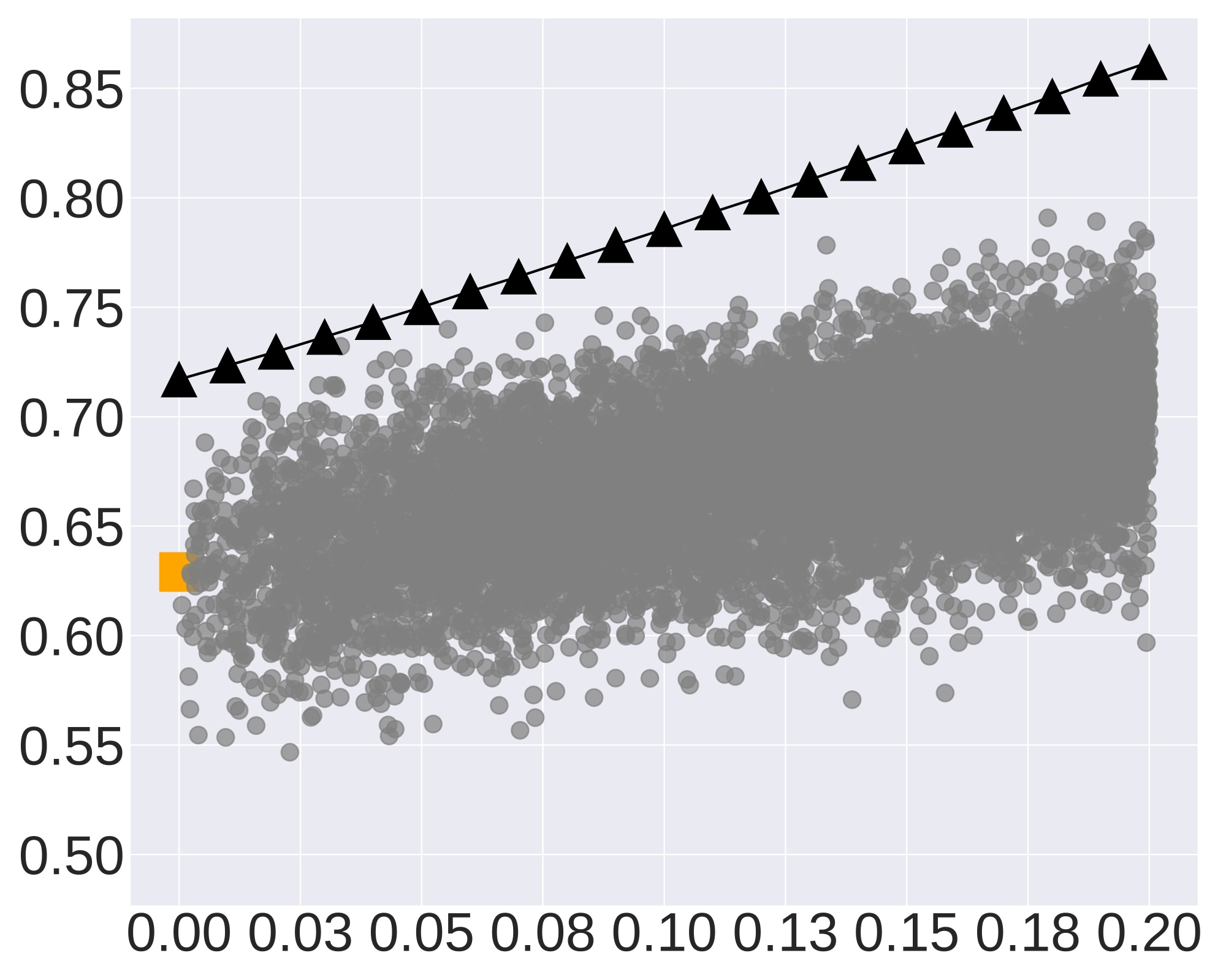
Refer to caption

   Hellinger Distance

 DART

Refer to caption

   Hellinger Distance

 E2E

Refer to caption

   Hellinger Distance

Refer to caption

Figure 12: Conformal generation risk α^ragsubscript^𝛼rag\hat{\alpha}_{\text{rag}} and empirical risks with Nrag=5,λg=20,λs=1.0formulae-sequencesubscript𝑁rag5formulae-sequencesubscript𝜆𝑔20subscript𝜆𝑠1.0N_{\text{rag}}=5,\lambda_{g}=20,\lambda_{s}=1.0 under distribution shifts for Biencoder-SFT.

 AESLC

Refer to caption

   # Generations λgsubscript𝜆𝑔\lambda_{g}

Evaluation Risk

 CommonGen

Refer to caption

   # Generations λgsubscript𝜆𝑔\lambda_{g}

 DART

Refer to caption

   # Generations λgsubscript𝜆𝑔\lambda_{g}

 E2E

Refer to caption

   # Generations λgsubscript𝜆𝑔\lambda_{g}

Refer to caption

Figure 13: Conformal generation risk α^ragsubscript^𝛼rag\hat{\alpha}_{\text{rag}} and simulated empirical risks for different generation set size λgsubscript𝜆𝑔\lambda_{g} and fixed Nrag=5,λs=1.0formulae-sequencesubscript𝑁rag5subscript𝜆𝑠1.0N_{\text{rag}}=5,\lambda_{s}=1.0 for Biencoder-SFT.

 AESLC

Refer to caption

   diversity threshold λssubscript𝜆𝑠\lambda_{s}

Evaluation Risk

 CommonGen

Refer to caption

   diversity threshold λssubscript𝜆𝑠\lambda_{s}

 DART

Refer to caption

   diversity threshold λssubscript𝜆𝑠\lambda_{s}

 E2E

Refer to caption

   diversity threshold λssubscript𝜆𝑠\lambda_{s}

Refer to caption

Figure 14: Conformal generation risk α^ragsubscript^𝛼rag\hat{\alpha}_{\text{rag}} and simulated empirical risks for different diversity threshold λssubscript𝜆𝑠\lambda_{s} with fixed Nrag=5,λg=20formulae-sequencesubscript𝑁rag5subscript𝜆𝑔20N_{\text{rag}}=5,\lambda_{g}=20 for Biencoder-SFT.

J.1 Experiment setup

Datasets

We evaluate C-RAG on four NLP datasets with retrieval augmented generation utilizing an external knowledge base. (1) AESLC: The Annotated Enron Subject Line Corpus (AESLC) dataset (Zhang & Tetreault, 2019) contains a collection of email messages from employees of the Enron Corporation. It contains two primary features: the “email_body“, which is the text of the email body, and the “subject_line“, which is the text of the email subject. The task is to generate the email subject given the email body. (2) The Generative Commonsense Reasoning (CommonGen) dataset (Lin et al., 2019) is a collection of commonsense descriptions, amounting to 79k descriptions over 35k unique concept sets, constructed via crowdsourcing and existing caption corpora. The task is to generate a sentence that uses given concepts in a coherent and commonsense way. (3) The Data Record to Text (DART) dataset (Nan et al., 2020) is a large-scale dataset designed to facilitate the generation of text from structured data records. It comprises 82,191 examples spanning various domains, with each example being a set of Resource Description Framework (RDF) triples derived from data records in tables and tree ontologies of schemas. These are annotated with sentence descriptions that encapsulate all the facts presented in the RDF triplet. (4) The End-to-End Generation (E2E) dataset (Novikova et al., 2017) contains about 50k comments in the restaurant domain. The task is to generate text from meaning representations (MRs), which are structured inputs that describe various aspects of a restaurant. These MRs consist of slots and values that a model needs to convert into natural language descriptions that are coherent and fluent.

External knowledge base: Following (Wang et al., 2023b; Wei et al., 2021; Cheng et al., 2023), we construct the external knowledge base as the union of a total of 30 publicly available datasets from 9 distinct categories with over 6 million documents.

Metrics

For generation tasks, we leverage ROUGE-L to quantify the quality of generations. ROUGE-L measures the longest common subsequence between a candidate generation and reference texts and is typically adopted for generation quality evaluations across the literature (Lin, 2004; Gatt & Krahmer, 2018). A low ROUGE-L implies poor quality generations and accordingly a high generation risk. Therefore, we adopt the risk function as 1ROUGE-L1ROUGE-L1-\text{ROUGE-L} to bound the risk in [0,1]01[0,1]. Note that C-RAG is agnostic to selection of risk functions, and thus, practitioners can specify any function that suits their specific use cases.

Retrieval models

We consider four types of retrieval models. (1) BM25 (Robertson et al., 2009) is a sparse encoding metric used to rank the candidate documents given a query in information retrieval tasks. BM25 scores are linearly weighted combinations of token-level scores and can be analytically formulated as a function of term frequency, inverse document frequency, and length of documents. (2) BAAI general embedding (BAAI/bge) (Zhang et al., 2023a) trains the SOTA embedding model in the MTEB benchmark (Muennighoff et al., 2022) and supports the diverse retrieval augmentation needs of LLMs by a reward formulation based on LLMs’ feedback, the stabilization of knowledge distillation, multi-task fine-tuning with explicit instructions, and homogeneous in-batch negative sampling. (3) OpenAI ada-text-embedding-02 (OpenAI/ada) is a close source text embedding models designed to convert text into high-dimensional vectors, which capture the semantic meaning of the input text and can be used for a variety of tasks, such as text similarity, classification, and clustering. (4) Biencoder-supervised fine-tuning (Biencoder-SFT) (Wang et al., 2023b) is a bi-encoder based dense retriever trained with contrastive loss and hard negative sampling strategies. It iteratively trains the retrieval model with hard negative samples identified by computing similarity scores by the current retrieval model.

Implementation details

We leverage Llama-7b for inference without specification. We perform conformal calibration on validation sets for different NLP datasets and fix the confidence levels 1δ=0.91𝛿0.91-\delta=0.9 across all evaluations. Lastly, we concatenate the retrieved in-context examples and the query sample with line break tokens.

J.2 Conformal risk bounds evaluation

Soundness and tightness of generation risk guarantees in C-RAG. To achieve the generation risk guarantee in Equation 1, C-RAG computes the upper confidence bound of generation risk by Proposition 1, which takes the empirical risk, calibration size and confidence level as input. We evaluate the conformal risks of RAG models αragsubscript𝛼rag\alpha_{\text{rag}} with variations of the number of retrieved examples Nragsubscript𝑁ragN_{\text{rag}} by calibration statistics on the validation set. To validate the soundness and tightness of the risk bounds, we randomly sample multiple test sets from a pool of test samples and compute the empirical risks on the sampled test sets. The sampling protocol is detailed in Algorithm 3 in Section J.2. We provide the results for OpenAI/ada, BM25, BAAI/bge, Biencoder-SFT in Figure 3. The results show that (1) the certified conformal risks αragsubscript𝛼rag\alpha_{\text{rag}} (black up-pointing triangles) are larger than the empirical risks of sampled test sets (grey points) and some empirical risks approach the risk bounds, demonstrating the soundness and tightness of risk bounds in C-RAG, and (2) the conformal risks decrease much as the number of retrieved examples Nragsubscript𝑁ragN_{\text{rag}} increases, which shows the effectiveness of retrieved in-context examples in RAG model and aligns with our theoretical analysis in Theorem 1.

Comparisons of C-RAG risk bounds for SOTA retrieval models. We also compare the conformal risk bounds of C-RAG for different retrieval models, including sparse encoding method BM25, and SOTA dense encoding models BAAI/bge, OpenAI/ada, Biencoder-SFT. The results in Figure 4 show that (1) RAG benefits in achieving a lower conformal risks of generations for different retrieval models, and (2) Biencoder-SFT is the most performant generally since the model is trained in the same domain as the test sets, while OpenAI/ada trained with an open corpus also demonstrates impressive effectiveness and even outperforms Biencoder-SFT on CommonGen dataset.

J.3 Conformal risk bounds evaluations under distribution shifts

Soundness and tightness of distribution-shifted conformal risk bounds in C-RAG. The test user input text can be out of the calibration distribution in practice, which needs correction of the conformal risk bounds considering the distribution drift. We provide the first distribution-shfted conformal risk bounds for general bounded risk functions in Theorem 2. We evaluate the bounds in Equation 6 as a function of the distribution shifting distance measured by Hellinger distance ρ𝜌\rho. To validate the bounds, we also construct various test sets with covariate shift induced by sample weight shifting. Specifically, different weights can be assigned to test samples in the shifted test sets and the Hellinger distance can also be explicitly computed by the original sample weights and shifted sample weights. We provide the detailed procedure in Algorithm 4 in Section J.3. We provide the results of conformal risk bounds and simulated empirical risks with Nrag=15subscript𝑁rag15N_{\text{rag}}=15 in Figures 8, 9 and LABEL:fig:bound_and_simulation_llmr_dist_shft with BM25, BAAI/bge, and Biencoder-SFT. The results demonstrate that (1) the distribution-shifted conformal risk bounds in Theorem 2 is sound and tight for different retrieval models, and (2) the conformal risk bounds increases linearly with the Hellinger distance and are non-trivial for a Hellinger distance up to 0.20.20.2.

Comparisons of C-RAG distribution-shifted risk bounds for SOTA retrieval models. We compare the distribution-drift conformal risk bounds for different retrieval models in Figure 10. The results show that (1) the bounds for different retrieval models increases linearly with a same slope as the Hellinger distance ρ𝜌\rho increases, and (2) Biencoder-SFT and OpenAI/ada demonstrate lower conformal risk bounds for different distances due to a lower initial risk without distribution shifts.

J.4 Conformal risk bounds with multi-dimensional RAG configurations

We already theoretically and empirically demonstrate the effectiveness of retrieved in-context examples quantified by Nragsubscript𝑁ragN_{\text{rag}}. To further improve the conformal risk bounds, we can addtionally consider more RAG parameters such as the number of generations λgsubscript𝜆𝑔\lambda_{g} in the generation set and a similarity threshold λssubscript𝜆𝑠\lambda_{s} to control the diversity of generations as Algorithm 1. We follow the RAG generation protocol in Algorithm 1 and define the risk function as the minimal risks among all candidate generations. We similarly construct random test sets and provide the results on DART and E2E in Figure 7. The results show that (1) the conformal risk bounds for multi-dimensional RAG configurations are still sound and tight, and (2) a larger Nragsubscript𝑁ragN_{\text{rag}} can reduce the conformal risks more sensitively compared to the number of generations λgsubscript𝜆𝑔\lambda_{g}, demonstrating the effectiveness of more retrieved in-context examples. We also fix the number of retrieved examples Nrag=5subscript𝑁rag5N_{\text{rag}}=5 and the diversity threshold λs=1.0subscript𝜆𝑠1.0\lambda_{s}=1.0, and evaluate the certified conformal risk and empirical risk of randomly sampled test set in Figure 13, which demonstrates that although not effective as the number of retrieved examples, a larger generation set size also benefits a low generation risk. Further more, we fix Nrag=5,λg=20,λs=1.0formulae-sequencesubscript𝑁rag5formulae-sequencesubscript𝜆𝑔20subscript𝜆𝑠1.0N_{\text{rag}}=5,\lambda_{g}=20,\lambda_{s}=1.0 and evaluate the risks for different distribution drift distance in Figure 12.

J.5 Valid configurations identification with specified risk levels

In conformal analysis (2) in Section 3.3, given a desired risk level α𝛼\alpha, C-RAG can certify a set of valid configurations Λ^αsubscript^Λ𝛼\hat{\Lambda}_{\alpha} such that any configuration in the set results in a conformal risk below α𝛼\alpha. We use Bonferroni correction for family-wise error rate control and evaluate empirical risks on randomly sampled test sets for the identified valid configurations. We provide the results on DART and ECE datasets in Figure 11. The results demonstrate that (1) the certification is empirically sound since the empirical risks of valid configurations Λ^αsubscript^Λ𝛼\hat{\Lambda}_{\alpha} are always below the desired level α𝛼\alpha, and (2) a large number of retrieved examples Nragsubscript𝑁ragN_{\text{rag}} and a large generation set size λgsubscript𝜆𝑔\lambda_{g} are effective in achieving a low generation risk since the valid configuration set includes the region with a large Nragsubscript𝑁ragN_{\text{rag}} and λgsubscript𝜆𝑔\lambda_{g}. We also individually demonstrate the effectiveness of generation set size λgsubscript𝜆𝑔\lambda_{g} and diversity threshold λssubscript𝜆𝑠\lambda_{s} in Figures 13 and 14.