The Matrix: A Bayesian learning model for LLMs

Abstract

In this paper, we introduce a Bayesian learning model to understand the behavior of Large Language Models (LLMs). We explore the optimization metric of LLMs, which is based on predicting the next token, and develop a novel model grounded in this principle. Our approach involves constructing an ideal generative text model represented by a multinomial transition probability matrix with a prior, and we examine how LLMs approximate this matrix. We discuss the continuity of the mapping between embeddings and multinomial distributions, and present the Dirichlet approximation theorem to approximate any prior. Additionally, we demonstrate how text generation by LLMs aligns with Bayesian learning principles and delve into the implications for in-context learning, specifically explaining why in-context learning emerges in larger models where prompts are considered as samples to be updated. Our findings indicate that the behavior of LLMs is consistent with Bayesian Learning, offering new insights into their functioning and potential applications.

1 Introduction

The advent of LLMs, starting with GPT3 [2], has revolutionized the world of natural language processing, and the introduction of ChatGPT [14] has taken the world by storm. There have been several approaches to try and understand how these models work, and in particular how “few-shot" or “in context learning" works [10, 11, 9], and it is an ongoing pursuit. In our work we look at the workings of an LLM from a novel standpoint, and develop a Bayesian model to explain their behavior. We focus on the optimization metric of next token prediction for these LLMs, and use that to build an abstract probability matrix which is the cornerstone of our model and analysis. We show in our paper that the behavior of LLMs is consistent with Bayesian learning and explain many empirical observations of the LLMs using our model.

1.1 Paper organization and our contributions

We first describe our approach at a high level, and in the rest of the paper get into the details of the approach. We focus on the optimization metric of these LLMs, namely, predict the next token, and develop the model from there on. We first describe the ideal generative text model (Section 2.1), and relate it to its representation of an abstract (and enormous) multinomial transition probability matrix. We argue that the optimization metric results in these LLMs learning to represent this probability matrix during training, and text generation is nothing but picking a multinomial distribution from a specific row of this matrix. This matrix, however is infeasible to be represented by the LLMs, even with billions of parameters, so the LLMs learn to approximate it. Further, the training data is a subset of the entire text in the world, so the learnt matrix is an approximation and reflection of the matrix induced by the training data, rather than the a representation of the ideal matrix. Next (Section 3), we relate the rows of this matrix to the embeddings of the prompt and prove (Theorem 3.1) a result on the continuity of the mapping between the embeddings and the multinomial distribution induced by the embedding. We then prove (Theorem 4.1) that any prior over multinomial distribution can be represented as a finite mixture of Dirichlet distributions. We then argue, and demonstrate (Section 5.2) that text generation by the LLMs is a Bayesian learning mechanism, where the probability distribution generated for the next token prediction is the posterior induced by the prompt as the new evidence, and the pre-trained model as the prior. We further relate the ability of the LLMs to learn completely new tasks, the so called in-context or few shot learning, to the (parameter) size of the LLMs and explain the emergent phenomena that has been observed for different kinds of in context learning. We finally present some implications of our model (Section 6) and conclude with open questions and directions to pursue (Section7). In the next section we start with a model for text generation/occurrence in the real world.

2 Text generation in the real world

2.1 The ideal generative text model

We start with an abstract model of the entire written text/knowledge that exists in the world, which we denote as $\mathcal{S}$. There is a finite vocabulary of the text, which we denote as $\mathcal{M}$, of size $|\mathcal{M}|=m$. Every word occurs with some probability $p_{i}$ in this corpus $\mathcal{S}$, with a multinomial distribution over the vocabulary $\mathcal{M}$, $(p_{1},p_{2},\cdots,p_{i},\cdots,p_{m})$ with a prior $u$. Suppose we pick a word randomly from this distribution, and say this word is “Protein". Now, again there will be a generated multinomial distribution $u(\cdot|\text{``Protein"})$ over the vocabulary $\mathcal{M}$ given that the first words is Protein. We denote this multinomial distribution as U(“Protein"). This multinomial distribution will be sparse (a very small subset of words will follow “Protein" over the vocabulary $\mathcal{M}$), and two words that will likely have a non-negligible probability are “synthesis" and “shake". If we sample the next words according to this multinomial distribution U(“Protein"), we will generate a posterior multinomial distribution U(“Protein synthesis") or U(“Protein shake") etc. The posterior multinomial distribution for U(“Protein synthesis") will be dominated by terms related to biology, whereas the posterior multinomial distribution U(“Protein shake") will be dominated by terms related to exercise and gym. And we keep progressing down this tree, as depicted pictorially in Figure 1.

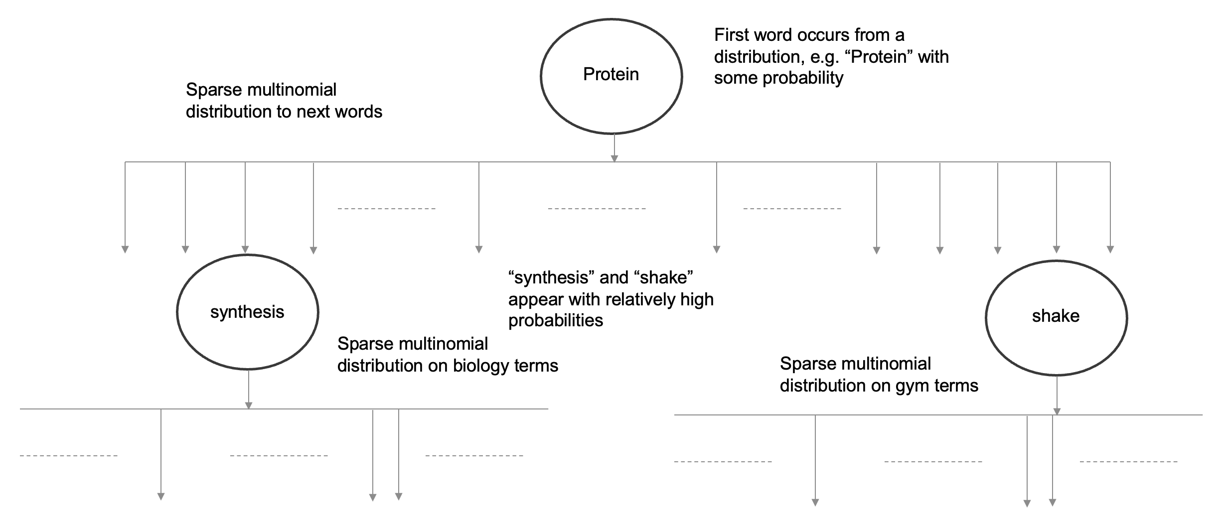
Figure 1: A conceptual model for text in the real world

Now we can view the entire text corpus $\mathcal{S}$ generating different multinomial probabilities for each sequence of words (or “prompts" as they are commonly referred to). If we consider a typical large language model (LLM) like ChatGPT, they will have a vocabulary of say 50,000 tokens (tokens are words/sub-words), and a prompt size that they respond to be about 8000 tokens. This results in a multinomial probability matrix of size $50000\times 50000^{8000}$ as depicted in Figure 2, where each row corresponds to a unique combination of 8000 tokens and each column is a token in the vocabulary of the LLM. This matrix is enormous, more than the number of atoms across all galaxies. Fortunately, it is very sparse in practice as an arbitrary combination of tokens is likely gibberish, and occurs with 0 probability. Even for rows that occur with non-negligible probability, the column entries in that row are also very sparse, since most entries of the multinomial distribution would be zero (“Protein synthesis" is unlikely to be followed by “convolutional networks" etc.). However, even with the row and column sparsity, the size remains beyond the capacity to accurately represent and so practical generative text models are built on several approximations, and we will go over them in the next section. At a fundamental level, LLMs are trying to compactly represent this Probability matrix, and given a prompt, they attempt to recreate the multinomial distribution in the row corresponding to the prompt. Note that these LLMs are trained to “predict the next token" as the objective function. With that objective function, the loss function used during training is the cross entropy loss function. It is straightforward to show that in the ideal scenario, the optimal multinomial distribution that they generate $\hat{u}(\cdot|\text{``Prompt"})$, should match the empirical multinomial distribution $u(\cdot|\text{``Prompt"})$ that exists in the training corpus $\mathcal{S}$, since the cross entropy $H(p,q)$ is minimized when $p\equiv q$. However, as stated earlier, this ideal is impossible to achieve in practice. In the next section we look at how LLMs work, and the approximations that are involved in practical settings.

Figure 2: Probability Matrix

2.2 Real world LLMs

In an abstract sense, Large Language Models (LLMs) work by using a given prompt to locate a specific row in the probability matrix. From this row, they extract a multinomial distribution, which then guides the selection of the next token by sampling from this distribution. As an example, for the prompt “The cat sat on the", the LLM generates a multinomial distribution as shown in Figure 3. The tokens “mat" and “couch" have the highest probabilities, and tokens “courage" or “the" have (extremely) low probabilities. This token is added to the prompt, and the process repeats, with the updated prompt leading to a new row in the matrix, continuing token generation in a sequential manner.

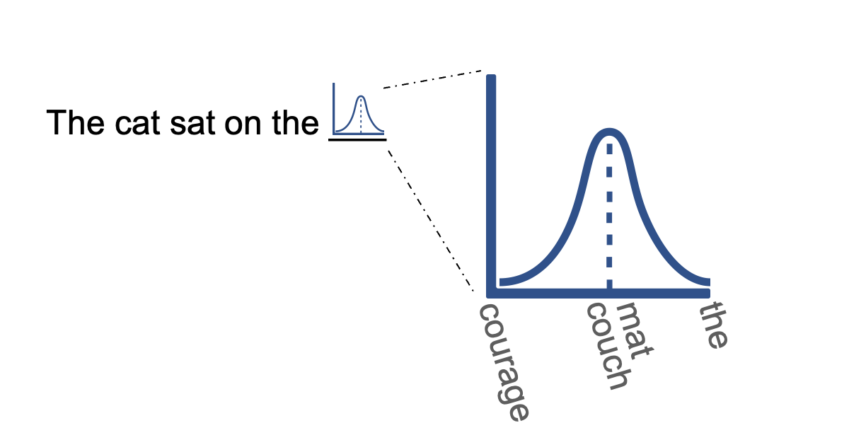
Figure 3: Multinomial distribution produced by an LLM in response to a prompt

The perfect probability matrix contains rows for all the text that is found (or can be generated) in the world, however, LLMs can only create an approximation of it using the training set, which is a subset, $\hat{\mathcal{S}}$, of the full corpus $\mathcal{S}$. The behavior of an LLM depends on the selection of $\hat{\mathcal{S}}$. So the first approximation that affects the performance of the LLMs is the incompleteness of the training set. A second approximation involves the the representation of the matrix that is generated from training on this incomplete set.

Figure 4: Functional blocks of an LLM based generative text system

The other approximation comes from representing text as embeddings. A short primer on how LLMs like gpt use embeddings for representation is as follows: LLMs begin processing text by converting sequences of characters or tokens into a fixed-dimensional space where each unique token is represented by a high-dimensional vector, known as an embedding. This representation captures semantic and syntactic properties of the language, enabling the model to understand the contextual relationships between tokens.

For instance in the transformer  [16] architecture the embeddings serve as the input layer, which employs an attention [1] mechanism to weigh the influence of different parts of the input text when predicting the next token. The attention mechanism allows the model to focus on relevant tokens for each prediction step, regardless of their position in the input sequence, thereby enabling the handling of long-range dependencies and variable-length input. This representation is then used downstream to generate the multinomial output distribution corresponding to the text input, however for our model in this paper we will abstract out the specifics of an architecture like the Transformer, and only assume that the input to the architecture is an embedding vector representing the prompt.

A decomposition of the functional blocks of an LLM based generative text model is shown in Figure  4. Text is entered by the user as a prompt, it is converted into embeddings by the LLM, then the LLM processes the embeddings as an input, produces an output multinomial distribution based on the embeddings and samples the next token from this distribution. The next token is appended to the prompt, converted into embeddings again and the process repeats until the next token picked corresponds to “end of response".

The key to understanding how In-Context learning or in general text generation works is to analyze how the networks respond to prompts and is similar to the question of generalization capabilities of classifiers in deep learning [7]. In the next sections we argue and demonstrate that all text generation in LLMs is consistent with a form of Bayesian learning, and In-Context learning is a special case of that.

3 Embeddings and Approximations

3.1 Preliminaries

In our model, each prompt has the corresponding representation in its embedding. Let $\mathscr{E}$ be the space of embeddings. For example $\mathscr{E}=\mathscr{R}^{r}$. We observe a finite number of embeddings, say $e_{1},...,e_{n}$ and each $e_{i}$ is mapped to a next token multinomial probability vector of the size of the vocabulary $m$, say $({p_{e}}_{i1},...,{p_{e}}_{im})$, ${p_{e}}_{ij}\geq 0,\sum{p_{e}}_{ij}=1$. Let the space of such probability vectors be $\mathscr{P}$. $\mathscr{E}$ is a metric space.

Suppose $T$ maps the embeddings to $\mathscr{P}$ by a convexity preserving transformation. That is, $T(\alpha e_{1}+(1-\alpha)e_{2})=\alpha T(e_{1})+(1-\alpha)T(e_{2})$. Consider the $\mathscr{L}_{p}$ metric for any $p\geq 0$ on $\mathscr{P}$. $T$ is clearly bounded in this metric by $1$.

3.2 Continuity

Theorem 3.1 (Continuity).

If the mapping $T$ is convexity preserving and bounded, then it is continuous.

Proof.

Consider any two points $x$ and $y$ in $\mathscr{E}$. Define $x_{\alpha}=\alpha y+(1-\alpha)x$. This defines a ray from $y$ to $x$. The corresponding $T$ mapping by the convexity preserving property is $\alpha T(y)+(1-\alpha)T(x)$. Clearly as $\alpha\rightarrow 0,\,x_{\alpha}\rightarrow x$ and $T(x_{\alpha})\rightarrow T(x)$ by the boundedness of $T(y)$. So the continuity is established along every ray. Now consider any arbitrary sequence $(x_{n},n=1,2,...)\rightarrow x$, then each of the point is on some ray to $x$. Thus establishing continuity for any sequence. ∎

The above theorem allows us to approximate any new multinomial distribution induced by an unseen embedding with the multinomial distributions induced by known embeddings as long as the operation is linear; for example by the nearest $k-means$ procedure.

Note that while we make this assumption about the convexity preservation mapping of embeddings to the multinomial distribution which leads to our continuity theorem, this property is important for the well-posedness of the posterior distribution in Bayesian statistics with respect to measurement errors, and has been shown in  [5]. Additionally, the convexity preserving property can be viewed as picking one embedding with probability $\alpha$, and the other with probability $1-\alpha$, and the linearity of expectation implies that the associated distributions induced by those embeddings also preserve the same weighting in expectation. Informally, this property leads to “well-behaved" LLMs that don’t have “wild" outputs.

4 Dirichlet approximation

We now show that any prior over multinomial distributions can be approximated as a finite mixture of Dirichlet distributions.

Theorem 4.1 (Dirichlet approximation).

Any distribution over $multinomial$ probabilities $u(p_{1},p_{2},\cdots p_{m})$ which has a continuous bounded density function can be approximated as a finite mixture of Dirichlet distributions.

Proof.

Consider a multinomial distribution on probabilities $P=(p_{1},p_{2},\cdots,p_{m}),\sum p_{i}=1.$ Now consider a fictitious experiment of generating $n$ observations from this multinomial distribution resulting in $x_{i}$ observations in $i^{th}$ category, $i=1,2,\cdot m$. Let $(\hat{P_{n}})=(x_{1},x_{2},\cdots,x_{m})/n)$, be the corresponding empirical probabilities. Then by the strong law of large numbers, $\hat{P_{n}}\rightarrow P\,a.s.$ Then, for any bounded continuous function,

$$E(u((\hat{P_{n}}))\rightarrow u(P)\,\mbox{uniformly in}\,P.\,\mbox{where },$$

$$E(u(\hat{P_{n}})) =\sum_{x_{1},\dots,x_{m}}u\left(\frac{x_{1}}{n},\frac{x_{2}}{n},\dots,\frac{x_{m}}{n}\right)$$

$$\quad\times\frac{\Gamma(n+1)}{\Gamma(x_{1}+1)\cdots\Gamma(x_{m}+1)}\prod_{i}p_{i}^{x_{i}}$$

Now let ${\mathcal{D}}(p|\alpha_{1},\alpha_{2},\dots,\alpha_{m})$ be a the density of an $m$ Dirichlet distribution with parameters $\alpha_{1},\alpha_{2},\dots,\alpha_{m}$. Then, the above can be simplified to show that:

$$E(u(\hat{P_{n}})) =\sum_{x_{1},\dots,x_{m}}u\left(\frac{x_{1}}{n},\frac{x_{2}}{n},\dots,\frac{x_{m}}{n}\right)$$

$$\quad\times\frac{\Gamma(n+1)}{\Gamma(n+m)}\mathcal{D}(p|x_{1}+1,x_{2}+1,\dots,x_{m}+1)$$

$$\quad\rightarrow u(p)$$

However, since $\int u(p)dp=1$, the integral of the middle term above also tends to $1$. Using this fact and normalizing it gives us:

$$\sum_{x_{1},\dots,x_{m}} u^{*}\left(\frac{x_{1}}{n},\frac{x_{2}}{n},\dots,\frac{x_{m}}{n}\right)$$

$$\times\mathcal{D}(p|x_{1}+1,x_{2}+1,\dots,x_{m}+1)\rightarrow u(p)$$

where,

$$u^{*}\left(\frac{x_{1}}{n},\frac{x_{2}}{n},\dots,\frac{x_{m}}{n}\right) =\frac{u\left(\frac{x_{1}}{n},\frac{x_{2}}{n},\dots,\frac{x_{m}}{n}\right)}{\sum_{x_{1},\dots,x_{m}}u\left(\frac{x_{1}}{n},\frac{x_{2}}{n},\dots,\frac{x_{m}}{n}\right)}$$

∎

The theorem is more general with appropriate regularity conditions. The convergence under the above conditions is in $L_{1}$ as well as in Total Variation in $p$ and the posteriors also converge. A special case of this is $Binomial$ distribution with $Beta$ prior, whereby any arbitrary prior for Binomial distribution can be approximated by a mixture of Beta distributions. Similar results apply to the general exponential family and for approximating a random probability measure by the mixtures of Dirichlet Processes [3].

Theorem 4.1 can lead to an efficient design of LLMs by identifying a small "basis set" by which any arbitrary $Multinomial$ distribution can be generated. It can help identify the right training set for a particular task that enables the creation of this basis set. Current practice of training LLMs is to use a mildly curated version of “the Internet" (wikipedia, reddit posts etc.) and a rigorous way to create the training set is needed.

5 Text generation and Bayesian learning

We argue that text generation by LLMs is consistent with a Bayesian learning process. When an LLM is fed a prompt, it goes through two steps. First, whatever current representation it has stored of the matrix, it locates the embeddings “closest" to the the embedding of the prompt, and the approximation via Theorems  3.1 and  4.1 of the multinomial distribution serves as the prior for the Bayesian learning. Next, the embedding of the prompt itself is treated as new evidence (likelihood) and the two are used to compute the posterior which is then used as the multiniomial distribution for the next token prediction. Note that if the prompt is an embedding the LLM has been trained on, then the Bayesian learning simply returns the prior distribution as the posterior (this is also the most efficient learning process during training, to minimize cross entropy loss). When the prompt contains something “new", the posterior adjusts to this new evidence. This process is depicted in Figure  5. How efficiently and accurately the posterior adjusts depends on the size of the LLM, and in the next subsections we show that In-Context learning within LLM models is consistent with Bayesian learning.

Figure 5: Conceptual Bayesian updating of next token multinomial probability

5.1 In Context Learning - Preliminaries

In-Context learning is a technique whereby task-specific responses are generated by giving task specific prompts to a LLM. There are many ways to do it, either by 0 shot or few shot learning. In-Context Learning can be classified in three broad categories according to [18]:

• Regular In Context Learning

• Flipped-Label In-Context Learning

• Semantically Unrelated In-Context Learning (SUIL)

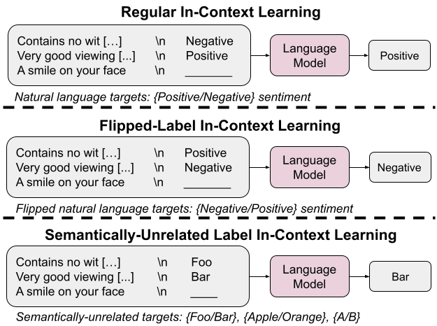
Figure 6: Types of In-Context Learning- from [18]

Basically, compared to the regular In-Context Learning, Flipped-Label In-Context Learning allows LLM prompts to have flipped labels so that the labels are opposite to the pre-trained LLM model. For example in the sentiment analysis task, “positive" is flipped to “negative" while prompting and vice versa. In Semantically Unrelated In-Context Learning (SUIL), “positive" is converted for example to “foo" and “negative" is converted to “bar"; both semantically unrelated in the pre-trained model.

What is surprising is that LLMs are able to deal with these inconsistencies and are able to adapt to the new labels rather quickly depending upon the number of parameters of the LLM. In the following sub-section we introduce the Bayesian paradigm using Dirichlet distributions and show how this behavior of LLM is consistent with the Bayesian Learning.

5.2 Bayesian Learning is In-context learning

We start with the simpler case of SUIL with two labels $A\,B$, where only one label is changed from $A$ to $B$. Since at any stage the auto-generation is done by the $multinomial$ distribution corresponding a row of the matrix, if we were to just consider the occurrence of the labels $A$ and $B$, the corresponding distribution will be a $Binomial(n,p)$ where $n$ is the sample size, and $p$ is the corresponding occurrence probability. For our exposition, besides assuming the occurrence of the labels $A,B$ is $Binomial$, for the Bayesian setting we further assume that it has a $Beta$ prior. The result in this section holds irrespective of this assumption since any prior distribution over $Binomial$ probability can be approximated by mixtures of $Beta$ priors as proven in Theorem 4.1. It also indicates that the entire development can be generalized to $multinomial$ distribution and $Dirichlet$ prior and mixtures of $Dirichlet$ priors when multiple labels are changed.

Recall that if $X\sim Bin(n,p)$ with the prior over $p$, $p\sim Beta(\alpha,\beta)$, and a fixed $n$, then,

$$p|n,x\sim Beta(\alpha+x,\beta+n-x)$$

with the corresponding posterior mean, $E(p|n,x)=(\alpha+x)/(\alpha+\beta+n)$, and the posterior variance $Var(p|x,n)=((\alpha+x)(\beta+n-x))/((\alpha+\beta+n)^{2}(\alpha+\beta+n+1))$ which is $O(n^{2})$. Further, $\alpha+\beta$ can be considered as the prior sample size of $A$ and $B$ , and $\alpha$ is the prior occurrence of $X_{A}$. See the related discussion in [4].

Now consider the most unrestricted case of the SUIL, namely, where the LLM is trained on the label $A$ with rare occurrences of the label $B$.

Consider now the auto-generated response conditional on $A$ occurring according to the training data of the base LLM. Then the training distribution for $A$ and $B$ can be represented as a Binomial distribution; $(p_{A},p_{B}),\,p_{A}+p_{B}=1$ with a prior for ($p_{A},p_{B})$ to be $Beta(\alpha_{A},\beta_{B})$. Since the training data from the LLM is mainly based on the label $A$ with a rare occurrence of $B$, we will have $\alpha_{A}\gg\beta_{B}$. Thus, $E(p_{A}|n=0)=\alpha_{A}/(\alpha_{A}+\beta_{B})\approx 1$ and $E(p_{B}|n=0)=\alpha_{B}/(\alpha_{A}+\beta_{B})\approx 0$. Further, since LLMs are trained on many labels, $\alpha_{A}$ would be relatively small, though much greater than $\beta_{B}$.

Now consider In-Context Learning for SUIL. Here we are replacing $A$ by $B$ in $n$ prompts, thus we have $x_{B}=n$ prompts of $B$ and $x_{A}=0$ prompts of $A$, all other context remaining the same. In this case

$$E(p_{A}|x_{A},x_{B})=\alpha_{A}/(\alpha_{A}+\beta_{B}+n),\,and,$$

$$E(p_{B}|x_{A},x_{B})=(\beta_{B}+n)/(\alpha_{A}+\beta_{B}+n)$$

So, clearly as the number of prompts $n$ for the label $B$ increases, $E(p_{B}|x_{A},x_{B})\rightarrow 1$ and $E(p_{A}|x_{A},x_{B})\rightarrow 0$.

We examine the qualitative behavior of this convergence, in the following table with $\alpha=0.3\,,\beta=0.01$. Here $\alpha_{A}/\beta_{B}=30$. As can be observed, with only three flipped examples, the posterior adjusts to nearly flip the probabilities of the labels from the pre-trained prior.

n	$E(p_{A}|n)$	$E(p_{B}|n)$
0	0.968	0.032
1	0.229	0.771
2	0.13	0.87
3	0.091	0.909

Table 1: Behavior of $E(p_{A}|n),E(p_{A}|n)$ with $n$ prompts and $\alpha=0.3\,\beta=0.01$

A similar behavior persists if $\alpha_{A}\ll n$. Further, to examine the asymptotic behavior consider

$$E(p_{A}|n)/E(p_{A}|n=0)=1/(1+n/(\alpha_{A}+\beta_{B})).$$

This suggests even if $\alpha_{A}\gg\beta_{B}$ resulting $E(p_{B}|n=0)\approx 0$, as long as $(\alpha_{A}+\beta_{B})$ is small, the In-Context Learning even in SUIL case will be very fast.

By analogy similar results hold for other categories of the In-Context Learning and also when multiple labels are being replaced. Finally, since Chain-of-Thought [17] learning is a type of In-Context Learning, the same results apply to it.

[18] empirically shows that the property of the adaptation to the Flipped-label In-Context Learning and SUIL depends upon the size of the model- the larger models learn better than smaller models. The Bayesian Learning also mimics this behavior by increasing $(\alpha_{A}+\beta_{B})$, that is increasing the prior sample size resulting in more peaked distribution around the labels. Table 2 shows with $\alpha=3\,\beta=0.1$. Here $\alpha_{A}/\beta_{B}$ still remains $=30$. Unlike the previous example, the posterior here is slow to adjust, and the probabilities of the two labels remain nearly equal after 3 examples whereas in the previous example they had nearly flipped.

n	$E(p_{A}|n)$	$E(p_{B}|n)$
0	0.968	0.032
1	0.732	0.268
2	0.588	0.412
3	0.492	0.508

Table 2: Behavior of $E(p_{A}|n),E(p_{A}|n)$ with $n$ prompts and $\alpha=3\,\beta=0.1$

This behavior can be intuitively explained since the larger models tend to have many more tokens and parameters, thus during the training they are acquiring more general knowledge scattering the probabilities across many more labels and parameters. This will result in smaller $\alpha_{A}+\beta_{B}$ for any two labels, and our model explains the emergence of In-Context learning with larger models, as observed in  [18] amongst others.

6 Implications of our model

In this section we present some implications of our model, beyond in context learning:

6.1 The importance of embeddings

We show that the performance of Bayesian learning in LLMs depends critically on the performance of the embeddings. Specifically we proved a “lipschitz-like" continuity property based on the assumption of convexity preserving mapping of embeddings to next token multinomial distributions, and a general result on the importance of continuity has been established in [5]. Embeddings are typically learnt as part of the LLM training process, called context-dependent  [15] but can also be independent of it. Our property implies that the embeddings of say words like “love" and “glove" be (sufficiently) far apart so that the semantic meaning is preserved in the mapping to the next token prediction probability distribution. This can be learnt by training purely on language. Sometimes, language models also train on world knowledge, and this implies the embeddings of say “Robert F Kennedy" and “Robert F Kennedy Jr." be far apart. However, mixing a world model with the language model can lead to unpredictable results and this needs to be carefully through through. It may be optimal to train LLMs and embeddings on only language and logic and introduce world models or knowledge primarily via the prompt and let the Bayesian posterior incorporate that knowledge into the generated text (a technique commonly known as retrieval augmented generation or RAG). However this needs to be explored and is part of our future work.

6.2 Chain of thought reasoning

Recently, Chain of Thought (CoT) reasoning [17, 13, 8] has been shown to be an effective way to increase the accuracy of answers from LLMs. This seems a natural consequence of the fact that if the LLMs break a problem into simpler steps, they are likely to have been trained on those simpler steps in some other context, and once the simpler step is generated for the current prompt, the LLM fits the embeddings closest to the steps it was trained earlier, and generates the corresponding multinomial distribution by the Bayesian learning process, as mentioned in Section 5.2. Without a step by step breakdown, it is possible that the LLM has not been trained (sufficiently) on similar inputs and hence the multinomial probability generated may not be accurate and hence Chain of Thought generally outperforms the vanilla prompt.

6.3 Deep Learning Architecture

In our work, we have treated the specific deep learning architecture as a black box that learns to efficiently encode the next token multinomial probabilities associated with embeddings found in the training corpus. The architecture that has dominated the LLM world in the past few years has been the Transformer, however recently structured state space models (SSMs) based models like Mamba  [6] have shown a lot of promise in addressing the computational inefficiencies of the Transformer model. Which architecture is optimal in terms of parameter efficiency or computational efficiency remains an intriguing open problem. From our standpoint, the critical feature of the LLMs is the predict the next token optimization metric coupled with the cross entropy loss during training which remains common across the various neural network architectures.

6.4 Hallucinations

One recurring issue with LLMs is that of hallucinations, where LLMs appear to make up stuff. Given the intended application of LLMs, creative text generation or serving facts, this can be either a feature or a bug. By viewing the LLM as essentially a map between the prompt embedding and the next token multinomial probability, we can reason about the “confidence" the LLM has in a generated answer. In particular, we can look at the entropy of the associated multinomial distribution of the picked token and make claims about hallucinations. In general, a lower entropy indicates a more peaked distribution and higher confidence in the answers. In the appendix we present a result, Theorem 8.2, that can serve as a guide to pick the next token to reduce entropy and increase confidence. A full treatment of the topic is beyond the scope of the current submission but gives a flavor of the kind of analysis possible with our framework. Note that the analysis is valid for any LLM that produces next token predictions, and is not dependent on any of our assumptions of Bayesian learning.

6.5 Large context size

Some LLMs like Claude from Anthropic and GPT4 have started providing extremely large context sizes (100K tokens for Claude, 128K tokens for GPT4). However, experimental evaluations of text generated by these LLMs indicate that the accuracy and recall of these LLMs with larger context is lower, keeping the parameter size constant. This again is explained by our model. If the LLM is attempting a compact representation of the large probability matrix, then going from a context size of 8000 (GPT 3.5) to 128 is an enormous increase in the row size of the matrix (from $50000^{8000}$ to $50000^{128000}$) and it is not surprising that the models are unable to retain the full context, the posterior computation happening over a much larger observable variable. The approximation needed becomes a lot more difficult for the LLMs handle. So while theoretically the LLMs have started accepting large context sizes, it is unlikely that the accuracy demonstrated by the shorter context models will be replicated by the larger context ones, using the same fundamental predict the next token architecture. It is however an interesting avenue to explore.

7 Conclusions

In this paper we present a new model to explain the behavior of Large Language Models. Our frame of reference is an abstract probability matrix, which contains the multinomial probabilities for next token prediction in each row, where the row represents a specific prompt. We then demonstrate that LLM text generation is consistent with a compact representation of this abstract matrix through a combination of embeddings and Bayesian learning. Our model explains (the emergence of) In-Context learning with scale of the LLMs, as also other phenomena like Chain of Thought reasoning and the problem with large context windows. Finally, we outline implications of our model and some directions for future exploration.

Impact Statement

This paper presents work whose goal is to advance the field of generative text models. There are many potential societal consequences of our work, none of which we feel must be specifically highlighted here.

8 Appendix

8.1 Entropy

The following theorem shows that as our prompts strengthens getting to a right answer, then the entropy and cross-entropy decreases. This result uses concepts of majorization and Schur-concavity [12].

8.2 Majorization and Schur-functions

We say $q$ majorizes $p$, i.e., $q\succ p$, if $q_{[1]}\geq p_{[1]}$, $q_{[1]}+q_{[2]}\geq p_{[1]}+p_{[2]}$, $q_{[1]}+...+q_{[i]}\geq p_{[1]}+...+p_{[i]}$ and $q_{[1]}+...+q_{[m]}=p_{[1]}+...+p_{[m]}$, where $p_{[i]}$ is the $i^{th}$ largest value of $(p_{1},...,p_{m})$. In what follows, $p\,and\,q$ are $multinomial$ probability vectors.

Note that if $q\succ p$ then $q$ is more peaked (concentrated) than $p$.

Definition 1 (Schur-convexity/concavity): A function $f$ is Schur-concave (Schur-convex) if it is permutation-invariant and $q\succ p$, then $f(q)\leq f(p)$ ($f(q)\geq f(p)$).

Definition 2 (T-transforms): Given $p$, $q=T_{\epsilon}(p)$ if $q=p$, except for some $i<j$ and some $\epsilon>0$ $q_{[i]}=p_{[i]}+\epsilon,\,and\,q_{[j]}=p_{[j]}-\epsilon$

we note the following results from [12]:

Theorem 8.1.

i) If $q=T_{\epsilon}(p)$, then $q\succ p$; ii) $q\succ p$ if only if there exist a series of T-transforms that transform $p$ in $q$

8.3 Entropy and Cross-Entropy

Given two $multinomial$ probability vectors $p\,\mbox{and}\,q$, recall that the cross-entropy of $q$ w.r.t. $p$ is defined as

$$CE(p,q)=-\sum_{i}p_{i}\log q_{i}=-\log\prod_{i}q_{i}^{p_{i}}$$

Note that $H(p)=CE(p,p)$ is the entropy of $p$ and $CE(p,q)\geq H(p)$

Now we state the main result:

Theorem 8.2 (Entropy and Cross-Entropy Reduction).

i) Entropy, $H$ is a Schur-concave function of $p$
ii) If $p\succ q$, $CE(p,q)$, cross-entropy of $q$ wrt $p$, is a Schur-concave function of $p$
iii) If $q\succ p$, $CE(p,q)$, the cross-entropy of $q$ wrt $p$, is a Schur-convex function of $q$

Proof.

Since the entropy and cross-entropy functions are permutation invariant, for simplifying notations we will assume that $p_{i}=p_{[i]}$ and $q_{i}=q_{[i]}$.

Suppose $q\succ p$, then by Theorem 2, $q$ is obtained by a series of T-transform of $p$. Thus, it is sufficient to prove the results by considering a single T-transform, $q=T_{\epsilon}(p)$, of $p$ where $q_{i}=p_{i}+\epsilon,\,and\,q_{j}=p_{j}-\epsilon,\,$ for some   $i<j$, that is $q\succ p$.

For i)

$$\frac{\partial H}{\partial\epsilon} =-\frac{(p_{i}+\epsilon)}{(p_{i}+\epsilon)}-\log(p_{i}+\epsilon)$$

$$\quad+\frac{p_{j}}{(p_{j}-\epsilon)}+\frac{(p_{i}-\epsilon)}{(p_{i}-\epsilon)}$$

$$\quad+\log(p_{j}-\epsilon)$$

Thus,

$$\operatorname{sign}\left(\frac{\partial H}{\partial\epsilon}\right) =\operatorname{sign}\left[-\log(p_{i})+\log(p_{j})\right]$$

$$\quad\text{which is negative since }p_{i}>p_{j}\text{ proving i)}.$$

For ii),

$$\partial CE(T_{\epsilon}(p),p)/\partial\epsilon=-\log(p_{i})+\log(p_{j})$$

Thus, $\operatorname{sign}(\partial CE(T_{\epsilon}(p),p)/\partial\epsilon=\log(p_{j}/p_{i})<0$ since $p_{j}<p_{i}$, proving ii)

For iii)

$$\partial CE/\partial\epsilon=-p_{i}/(p_{i}+\epsilon)+p_{j}/(p_{j}-\epsilon)$$

Thus,

$$\operatorname{sign}\left(\frac{\partial CE}{\partial\epsilon}\right) =\operatorname{sign}\left[-p_{i}(p_{j}-\epsilon)+p_{j}(p_{i}+\epsilon)\right]$$

$$=\operatorname{sign}\left(p_{i}+p_{j}\right)\cdot\epsilon$$

$$>0\,\text{proving (iii)}$$

∎

This implies that if $q$ is more concentrated then $p$, then entropy decreases. The more confident the LLM is of an answer, the more deterministic is the multinomial distribution, i.e. lower entropy. So picking the next token according to the majorization criterion results in decreasing entropy and more confident answers by the LLM.

References

- [1] Dzmitry Bahdanau, Kyunghyun Cho, and Yoshua Bengio. Neural machine translation by jointly learning to align and translate. In The International Conference on Learning Representations (ICLR), 2015.
- [2] Tom B. Brown, Benjamin Mann, Nick Ryder, Melanie Subbiah, Jared Kaplan, Prafulla Dhariwal, Arvind Neelakantan, Pranav Shyam, Girish Sastry, Amanda Askell, Sandhini Agarwal, Ariel Herbert-Voss, Gretchen Krueger, Tom Henighan, Rewon Child, Aditya Ramesh, Daniel M. Ziegler, Jeffrey Wu, Clemens Winter, Christopher Hesse, Mark Chen, Eric Sigler, Mateusz Litwin, Scott Gray, Benjamin Chess, Jack Clark, Christopher Berner, Sam McCandlish, Alec Radford, Ilya Sutskever, and Dario Amodei. Language models are few-shot learners. CoRR, abs/2005.14165, 2020.
- [3] S. R. Dalal. A note on the adequacy of mixtures of dirichlet processes. Sankhyā: The Indian Journal of Statistics, Series A (1961-2002), 40(2):185–191, 1978.
- [4] S. R. Dalal and W. J. Hall. Approximating priors by mixtures of natural conjugate priors. Journal of the Royal Statistical Society. Series B (Methodological), 45(1):90–97, January 1983.
- [5] Emanuele Dolera and Edoardo Mainini. Lipschitz continuity of probability kernels in the optimal transport framework, 2023.
- [6] Albert Gu and Tri Dao. Mamba: Linear-time sequence modeling with selective state spaces, 2023.
- [7] K. Kawaguchi, Y. Bengio, and L. Kaelbling. Generalization in deep learning. In Mathematical Aspects of Deep Learning, pages 112–148. Cambridge University Press, dec 2022.
- [8] Andrew K. Lampinen, Ishita Dasgupta, Stephanie C.Y. Chan, Kory Matthewson, Michael Henry Tessler, Antonia Creswell, James L. McClelland, Jane X. Wang, and Felix Hill. Can language models learn from explanations in context? arXiv preprint arXiv:2204.02329, 2022.
- [9] Liunian Harold Li, Jack Hessel, Youngjae Yu, Xiang Ren, Kai-Wei Chang, and Yejin Choi. Symbolic chain-of-thought distillation: Small models can also "think" step-by-step. arXiv preprint arXiv:2306.14050, 2023.
- [10] Hunter Lightman, Vineet Kosaraju, Yura Burda, Harri Edwards, Bowen Baker, Teddy Lee, Jan Leike, John Schulman, Ilya Sutskever, and Karl Cobbe. Let’s verify step by step. arXiv preprint arXiv:2305.20050, 2023.
- [11] Bingbin Liu, Jordan T Ash, Surbhi Goel, Akshay Krishnamurthy, and Cyril Zhang. Transformers learn shortcuts to automata. arXiv preprint arXiv:2210.10749, 2022.
- [12] Albert W. Marshall and Ingram Olkin. Theory of Majorization and Its Applications. Academic Press, 1979.
- [13] Sharan Narang, Colin Raffel, Katherine Lee, Adam Roberts, Noah Fiedel, and Karishma Malkan. WT5?! Training text-to-text models to explain their predictions. arXiv preprint arXiv:2004.14546, 2020.
- [14] OpenAI. Chatgpt: Optimizing language models for dialogue. https://www.openai.com/chatgpt, 2023. Accessed: 2023-11-08.
- [15] Matthew E. Peters, Mark Neumann, Mohit Iyyer, Matt Gardner, Christopher Clark, Kenton Lee, and Luke Zettlemoyer. Deep contextualized word representations. In Marilyn Walker, Heng Ji, and Amanda Stent, editors, Proceedings of the 2018 Conference of the North American Chapter of the Association for Computational Linguistics: Human Language Technologies, Volume 1 (Long Papers), pages 2227–2237, New Orleans, Louisiana, June 2018. Association for Computational Linguistics.
- [16] Ashish Vaswani, Noam Shazeer, Niki Parmar, Jakob Uszkoreit, Llion Jones, Aidan N Gomez, Ł ukasz Kaiser, and Illia Polosukhin. Attention is all you need. In I. Guyon, U. Von Luxburg, S. Bengio, H. Wallach, R. Fergus, S. Vishwanathan, and R. Garnett, editors, Advances in Neural Information Processing Systems, volume 30. Curran Associates, Inc., 2017.
- [17] Jason Wei, Xuezhi Wang, Dale Schuurmans, Maarten Bosma, Brian Ichter, Fei Xia, Ed Chi, Quoc Le, and Denny Zhou. Chain-of-thought prompting elicits reasoning in large language models, 2023.
- [18] Jerry Wei, Jason Wei, Yi Tay, Dustin Tran, Albert Webson, Yifeng Lu, Xinyun Chen, Hanxiao Liu, Da Huang, Denny Zhou, and Tengyu Ma. Larger language models do in-context learning differently, 2023.