Is Mamba Capable of In-Context Learning?

Abstract

This work provides empirical evidence that Mamba, a newly proposed selective structured state space model, has similar in-context learning (ICL) capabilities as transformers. We evaluated Mamba on tasks involving simple function approximation as well as more complex natural language processing problems. Our results demonstrate that across both categories of tasks, Mamba matches the performance of transformer models for ICL. Further analysis reveals that like transformers, Mamba appears to solve ICL problems by incrementally optimizing its internal representations. Overall, our work suggests that Mamba can be an efficient alternative to transformers for ICL tasks involving longer input sequences.

1 Introduction

Recent advancements in large-scale neural language modeling (Brown et al., 2020) have demonstrated that Transformer models (Vaswani et al., 2017) exhibit in-context learning (ICL) capabilities: after (self-supervised) pre-training, they can infer how to perform tasks only from input examples without the need for explicit training nor fine-tuning. This ability represents a departure from established in-weights learning of traditional machine learning and has sparked considerable academic interest. In contrast to meta-learning approaches (Hospedales et al., 2021), in transformer models ICL emerges from pre-training: without explicit training on a distribution of tasks and without having any specific inductive bias. Recent studies advanced the understanding of how transformers can implement and learn (variants of) in-context gradient descent when trained on distributions of simple supervised learning tasks, e.g., on linear regression tasks (Von Oswald et al., 2023; Ahn et al., 2023; Bai et al., 2023). Despite such results, whether pre-trained transformers perform in-context gradient descent on more complex tasks remains an ongoing discussion (Shen et al., 2023).

Orthogonal to these investigations into the transformer architecture, recent work proposed deep state space models to overcome limitations of transformers in processing long sequences (Tay et al., 2021), such as S4 (Gu et al., 2021a) or H3 (Gu et al., 2021b). In essence, these models merge elements from recurrent and convolutional networks with state space approaches (Kalman, 1960). However, their success on NLP tasks was limited due to problems handling dense information tasks.

This works conducts an investigation into the ICL capabilities of the recently proposed Mamba architecture (Gu & Dao, 2023), a successor to S4 and H3. Mamba has already shown its potential in different applications beyond NLP, such as (visual) representation learning (Zhu et al., 2024) or image segmentation (Ma et al., 2024). Concurrent to our work, the ICL capabilities of Mamba were investigated on synthetic language learning tasks by Akyürek et al. (2024). Our work is orthogonal to theirs, as we provide ICL results for both regression and NLP tasks, and additionally conduct a probing analysis on the representations at intermediate layers to better understand Mamba’s ICL solution mechanisms (for simple function classes).

Our analysis provides the following contributions to understanding Mamba’s ICL capabilities:

• We demonstrate that Mamba is capable of ICL and performs on-par with transformers in many cases This highlights Mamba as an efficient alternative to transformers for ICL tasks entailing longer sequences. In addition, we find that Mamba outperforms its predecessor S4, and a recent Recurrent Neural Network (RNN) architecture, RWKV (Peng et al., 2023).

• Using a simple probing approach, we provide preliminary insights into the mechanism by which Mamba incrementally solves ICL tasks. We find that the optimization processes exhibited by Mamba bear similarities to those of transformer models.

Outline  We begin by establishing Mamba’s ICL capabilities on simple function classes (Garg et al., 2022) in Section 2, comparing it to a causal transformer model in Section 2.1. Having established that Mamba is capable of ICL, we aim to understand its internal mechanisms to perform ICL in Section 2.2. To this end, we analyze how Mamba incrementally approximates the solution of the in-context task. Finally, we study Mamba’s ICL performance on more complex NLP in-context tasks from Hendel et al. (2023) in Section 3.

2 Investigation of Simple Function Classes

We followed the experimental protocol of Garg et al. (2022): each model is trained on a task distribution and then tested on the same distribution. This process was repeated for 3 regression task distributions, each falling into a specific function class: linear functions, 2-layer ReLU neural networks, and decision trees. Models trained on linear functions were also tested on out-of-distribution (OOD) tasks. Differently from Garg et al. (2022), we also tested the models on tasks with more input examples than seen during training, to test if they can extrapolate to longer inputs. Details on each task distribution are provided in Section A.2.3.

We compare Mamba to a causal transformer model using the GPT2 architecture (Radford et al., 2019), S4 and some baselines specific to each function class (see Section A.2.4). We intentionally compare to S4, a predecessor to Mamba, as it is a linear-time invariant model: its state dynamics are linear and constant through time. In contrast, Mamba is a linear time variant model: its state dynamics can change based on the current input. For architectural details on Mamba see Section A.1. To ensure a fair comparison, the architecture of Mamba and S4 is adjusted to have a comparable number of parameters to the transformer (9.5 M). For further training details we refer to Section A.2.1.

We removed the positional embedding used in the causal transformer by Garg et al. (2022), since we observed that it hinders the transformer’s ability to extrapolate to longer inputs, as also shown by Press et al. (2021). Similar to Müller et al. (2021), we argue this to be more natural in the present setup as the input is actually a set of data points, not a sequence.

To sample the inputs of each training task for linear regression, Garg et al. (2022) used a normal distribution, while we used a skewed Gaussian distribution. Our findings show that this improves robustness w.r.t. OOD tasks of both Mamba and transformers. Formally, we trained on linear functions of the form $F=\{f\,:\,f(x)=w^{T}x,w\in\mathbb{R}^{d}\}$ with input dimension $d=20$. For each training task, we sampled $w$ from an isotropic Gaussian $\mathcal{N}(0,I_{d})$ and $x_{1},\dots,x_{k},x_{k+1}$ from $\mathcal{N}(0,\Sigma)$, where $\Sigma$ is a skewed covariance matrix with its eigenbasis chosen at random and the $i$th eigenvalue proportional to $1/i^{2}$. Following this, we set $y_{i}=w^{T}x_{i}$ and assembled the input prompt $P=(x_{1},y_{1},x_{2},y_{2},...,x_{k},y_{k},x_{k+1})$. We used the mean squared error $\frac{1}{k+1}(\hat{y}_{i}-y_{i})^{2}$ as loss function, where $\hat{y}_{i}$ is the output of the model corresponding to $x_{i}$.

2.1 Analysis of in-distribution and out-of-distribution performance

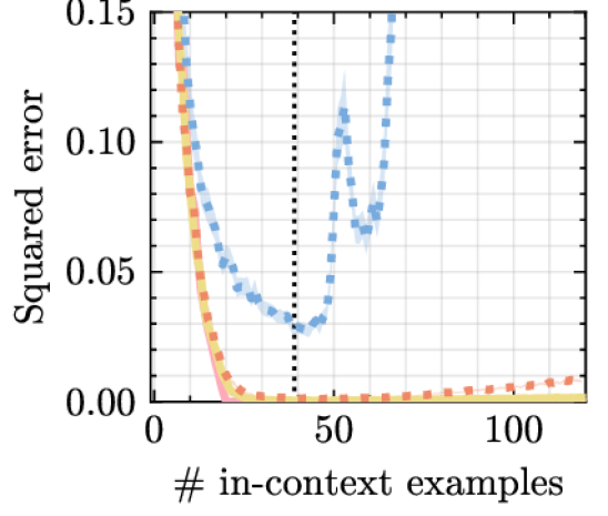
(a) Skewed LR

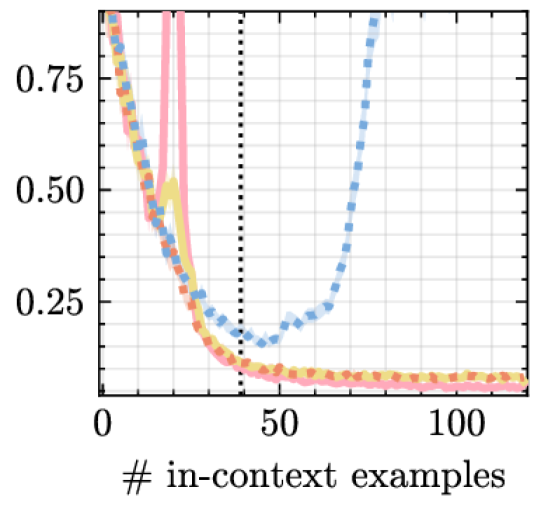
(b) Noisy LR

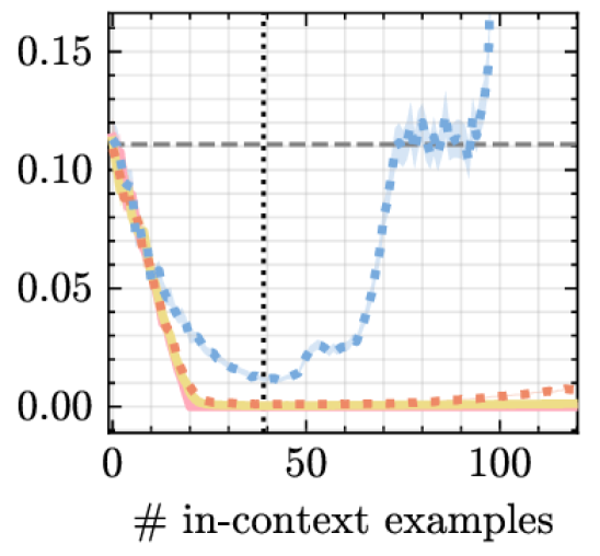
(c) x-scale 0.333

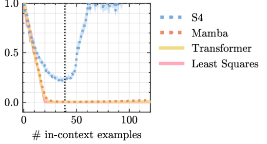
(d) Random quadrants ————–

Figure 1: Comparative visualization of Mamba, S4, and transformer models trained on skewed linear regression and evaluated in-distribution (a) and out-of-distribution (b) - (d). The dotted vertical line indicates the number of in-context examples used for training.

Figure 1 shows our results for models trained on skewed linear regression tasks. Both Mamba and the transformer model are capable to solve the in-distribution and out-of-distributions tasks, while S4 is unable to do so. We find that Mamba’s ICL performance deteriorates more than that of the transformer as the number of in-context examples increases. We hypothesize that S4’s poor ICL performance is due to its linear time invariance. A similar hypothesis was also drawn by Gu & Dao (2023) for the task of selective copying. Besides that, both Mamba and Transformers exhibit input length extrapolation on noisy linear regression: the performance improves with more than 40 in-context examples.

Section A.2.5 provides further results for Mamba and the transformer model on decision trees and 2-layer ReLU neural networks regression tasks perform comparably when evaluated in-distribution (Figures 5(c) and 5(b)), while when trained on non-skewed linear regression tasks they are less robust to OOD tasks (Figure 6), even if they both perform well in-distribution (Figure 5(a)).

2.2 Mechanistic understanding via probing

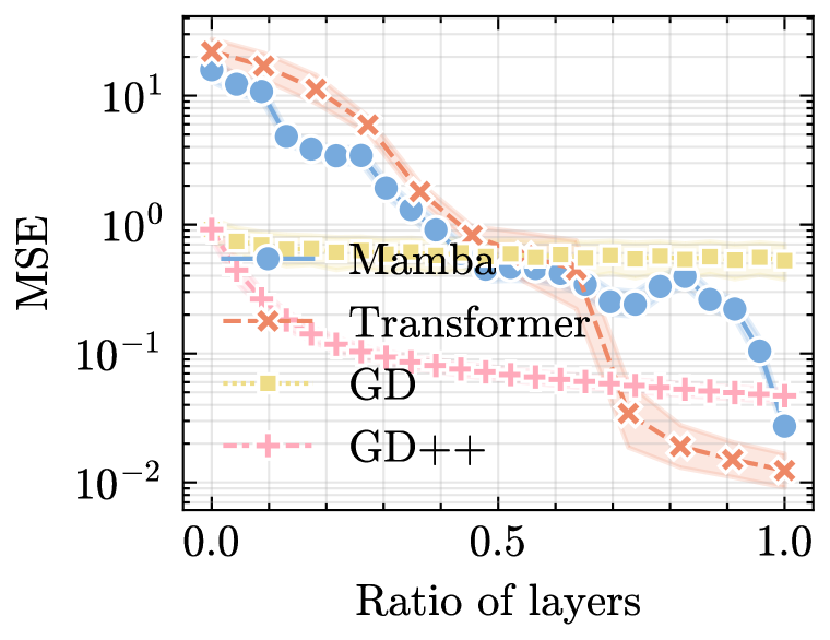
(a) Skewed Linear Regression

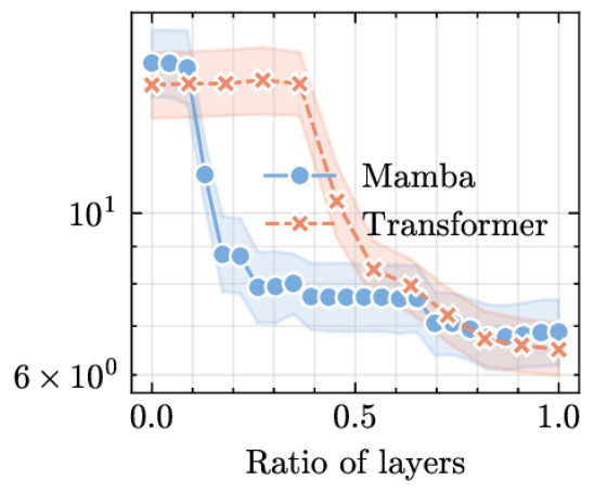
(b) ReLU Neural Network

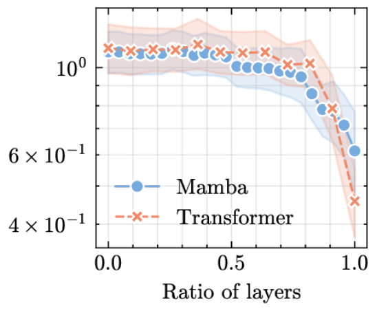
(c) Decision Tree

Figure 2: ICL ’Learning curves’ depicting the iterative optimization performance of Mamba and Transformer models on three regression tasks.

To better understand how the Mamba and transformer models perform ICL, we aim to test if they both employ a solution strategy akin to iterative optimization, i.e., study if they incrementally improve their solutions layer after layer (Von Oswald et al., 2023; Ahn et al., 2023; Bai et al., 2023).

We adopted a probing strategy similar to the one by (Geva et al., 2021) for transformer language models. Differently from other probing strategies like the one by Akyürek et al. (2023), who learn a (non-linear) probe on the high-dimensional intermediate representations, this strategy first passes the intermediate representations through the decoder at the end of transformer model used to map from the embedding to the output space (see Section A.2.6). The decoding procedure of Mamba is similar to the transformer, but includes a layer norm. To account for possible differences in scale and shift, we estimated a linear probing model on the in-context example data using least squares between the predictions and the regression target. We argue this to be a less biased probing strategy, since in our setup it reduces the degrees of freedom of the probe to just $2$ parameters per task: scale and shift.

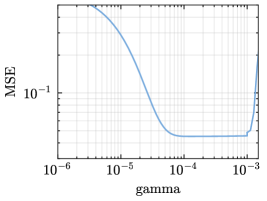
Figure 7: Results for grid search over $\gamma$ for GD++. We optimized $\gamma$ in order to have optimal performance of GD++ at iteration 24 (the same number of iterations reported in Figure 2(a)). We picked a value of

We conducted the probing analysis on transformers and Mamba models trained on skewed linear regression, ReLU neural networks, and decision trees. For skewed linear regression, we additionally compared to Gradient Descent (GD) and GD⁺⁺ as done in Von Oswald et al. (2023). GD⁺⁺ is a version of preconditioned gradient descent in which the data samples undergo a transformation ($x_{i}\leftarrow(I-\gamma XX^{T})x_{i}$) and we tuned $\gamma$ for optimal performance via a grid search (c.f., Figure 7 in Appendix), while the step-size was set for each task to the theoretically optimal value, i.e., as $2/(L+\mu)$, where $L,\mu$ are the largest and smallest eigenvalues of the empirical covariance matrix of the task.color=violet!20,]RG: Is this true?, JS: Yes We ran GD and GD⁺⁺ for 24 iterations to match the 24 layers of our Mamba model.

Figure 2 provides strong evidence to the hypothesis that both Mamba and the transformer employ an iterative solution scheme on the linear regression task, since the log-MSE decreases (almost) linearly. For ReLU neural networks and decision trees, the results are more ambiguous and further investigations are required, since the error decreases more abruptly, albeit sometimes decreasing gradually, and the final error is still relatively high. We also note that intermediate predictions for all three tasks achieve similar MSE. The comparison between GD, GD⁺⁺, Mamba, and the transformer in Figure 2(a) reveals that GD⁺⁺ achieves a performance level similar to Mamba, while GD shows slower convergence also due to the tasks having skewed covariance. Interestingly, the transformer model outperforms GD⁺⁺.

Finally, we compared the scalar scale and shift estimated by the linear probing model for Mamba and transformer in Figure 8 in the Appendix. Interestingly, we find that the linear probing model only makes small adjustments for linear regression and ReLU neural network, with scales close to one and shifts close to zero.

3 Investigation of Simple NLP Tasks

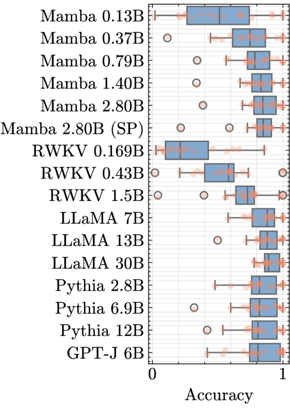
Figure 3: Accuracy of Mamba variants compared to RWKV and other transformer-based models on in-context NLP tasks.

In this section, we evaluated the ICL performance of various pre-trained Mamba language models, with parameter counts from 130 million to 2.8 billion.

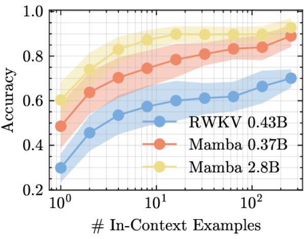
Figure 4: Average task accuracy for increasing context length. Reported are the 5/95% confidence intervals.

The pre-training for all variants was done on the Pile dataset (Gao et al., 2020), while the Mamba 2.8B (SP) checkpoint underwent further fine-tuning on ca. 600 billion tokens from the SlimPajama dataset.

We compared the Mamba variants to another RNN model with linear state dynamics named RWKV (Peng et al., 2023), which was also pre-trained on Pile, and popular transformer-based language models, such as LLama (Touvron et al., 2023), Pythia (Biderman et al., 2023), and GPT-J 6B (Wang & Komatsuzaki, 2021). We did not compare to S4 because we are not aware of S4 models pretrained on Pile.

We followed the experimental protocol of Hendel et al. (2023), which tested 27 NLP tasks spanning a wide range of categories, including algorithmic tasks (e.g., list element extraction), translation (e.g., English to Spanish), linguistic tasks (e.g., singular to plural conversion), and knowledge-based tasks (e.g., identifying country-capital pairs). For evaluation, we used the same datasets as Hendel et al. (2023) except for the algorithmic tasks, which were randomly generated (we use the same generation parameters). We report the mean accuracy over 400 generated test sets per task, each having five in-context examples.

Figure 3 shows that ICL performance improves for all models with increasing number of parameters. Notably, Mamba 2.8B achieves a ICL accuracy close to LLama 7B, and on par with GPT-J and Pythia models. In addition, we find that Mamba consistently outperforms the similarly scalable RWKV at comparable parameter sizes. We provide a detailed table of per-task accuracies in Appendix A.3.

Finally, we find that Mamba scales well with the number of in-context examples; see Figure 4. Particularly, Mamba 0.37B and 2.8B maintain a considerable performance edge over RWKV 0.43B.

4 Conclusions

In this work, we have demonstrated that the recently proposed Mamba architecture is capable of effective ICL across tasks involving simple function approximation as well as more complex natural language processing problems. Our analysis showed that Mamba performs on par with transformer models, while also outperforming the S4 and RWKV baselines. We provide initial evidence that Mamba appears to solve ICL problems by incrementally refining its internal representations in a manner akin to an iterative optimization strategy, as transformer do. Overall, our findings establish Mamba as an efficient and performant alternative to transformers for ICL involving longer input sequences.

5 Acknowledgements

We would like to thank Alma Lindborg, André Biedenkapp and Samuel Müller (alphabetic order) for their constructive feedback in preparation of this paper.

This work was supported in part by the European Union – NextGenerationEUPNRR MUR, EU project 101070617 entitled “European Lighthouse on Secure and Safe AI”, and EU project 101120237 entitled “European Lighthouse of AI for Sustainability”

This work was partially funded by the Deutsche Forschungsgemeinschaft (DFG, German Research Foundation) under grant number 417962828, and the Bundesministerium für Umwelt, Naturschutz, nukleare Sicherheit und Verbraucherschutz (BMUV, German Federal Ministry for the Environment, Nature Conservation, Nuclear Safety and Consumer Protection) based on a resolution of the German Bundestag (67KI2029A)

The authors acknowledge support by the state of Baden-Württemberg through bwHPC and the German Research Foundation (DFG) through grant no INST 39/963-1 FUGG. We acknowledge funding by the European Union (via ERC Consolidator Grant DeepLearning 2.0, grant no. 101045765). Views and opinions expressed are however those of the author(s) only and do not necessarily reflect those of the European Union or the European Research Council. Neither the European Union nor the granting authority can be held responsible for them.

Appendix A Appendix

A.1 Mamba Architecture

The Mamba architecture (Gu & Dao, 2023) is a sequence model that uses Structured State Space Models (SSMs) as its core building block. SSMs are recurrent neural networks with an high-dimensional latent state and linear state dynamics that feature also a “convolutional mode” which allows to parallelize the training training in a way similar to transformer models. Compared to previous SSMs, Mamba primary innovation is the introduction of a selection mechanism that makes the SSM parameters functions of the input, enabling selective propagation of information.

However, this selection mechanism poses a challenge for efficient convolutions. To address this, Mamba leverages a hardware-aware recurrent algorithm that exploits the GPU memory hierarchy, avoiding the need to materialize the full latent states in the GPU high bandwidth memory. Mamba’s architecture is designed to balance the trade-off between efficiency and effectiveness in sequence models by effectively compressing the input context into the latent state through selectivity.

Overall, the latent state in Mamba is updated as follows:

$$h_{t} =\bar{A}(\Delta(x_{t}))h_{t-1}+\bar{B}(x_{t},\Delta(x_{t}))x_{t}\quad,$$

$$y_{t} =\bar{C}(x_{t})h_{t}\quad,$$

where $h_{t}$, $x_{t}$ and $y_{t}$ are the current hidden states, current input and output respectively $\Delta,\bar{A},\bar{B},\bar{C}$ are specific parametric functions learned through backpropagation. See Gu & Dao (2023) for further details on Mamba’s architecture.

Mamba is referred to as linear time variant because $h_{t}$ is a linear function of $h_{t-1}$, but the linear transformation depends on the current input $x_{t}$. In contrast, previous SSM models, such as S4 and H3, were linear time invariant, since $\bar{A}$, $\bar{B}$ and $\bar{C}$ are not dependent on the current input.

A.2 ICL for simple function classes

We follow the experimental setup of Garg et al. (2022) by building on their MIT-Licensed code at https://github.com/dtsip/in-context-learning.

A.2.1 Model parameters

As in Garg et al. (2022), we used a GPT-2 (Radford et al., 2019) model with embedding size 256, 12 layers and 8 heads, resulting in 9.5 million parameters. As mentioned in the main text, we removed the positional embedding to improve the input length extrapolation. We set Mamba’s $D$ parameter to $256$, matching the transformer’s embedding dimension, while we set the number of Mamba’s layers to $24$, doubling the ones of the transformer ($12$). This is done because each Mamba block can be roughly seen as the fusion of a MLP and SSM, and has roughly half the number of parameters of a transformer block, which can be divided into an MLP and an attention part. For a fair comparison, S4 also uses $24$ layers, however we set the embedding size to 435 to match the 10 million parameters of Mamba and the transformer. We note that a similar comparison between S4 and transformer models, also testing for input length extrapolation, was done by  Lee et al. (2023). However, we used models with substantially more parameters (10 million vs. 500 thousand) and transformers without positional encoders.

A.2.2 Training details

We adopted the same experimental setup used for the transformer model by (Garg et al., 2022) for Mamba, the transformer, and S4. At each training step, we computed the loss on a mini-batch of 64 prompts, each corresponding to a task sampled from a task distribution. We used no dropout in our experiments. We adopt a curriculum learning strategy: starting with training points of the lower-dimensional subspace and fewer input examples per prompt, and increasing the dimensionality of the subspace and the number of in-context examples every 2000 steps. For more details on the training, we refer to (Garg et al., 2022, A.2 Training).

For Mamba, we used the same learning rate used by Garg et al. (2022) for the transformer model (which is the only one we tried), which means that both Mamba and the transformer model undergo exactly the same training conditions. For S4 instead, we searched for the optimal learning rate in [1e-5, 1e-4, 1e-3, 1e-2] and selected 1e-3, which we found to achieve the lowest average loss on the query point at the end of training.

A.2.3 Simple task distributions

Below, we describe how tasks are sampled for each task distribution that we considered. Task distributions are the same ones as in Garg et al. (2022).

For each task we first sampled $x_{1},\dots,x_{k},x_{k+1}$ input points Then, for each point we sampled the output $y_{i}$ as a function of $x_{i}\in\mathbb{R}^{d}$, possibly adding noise. Finally, the prompt $P=x_{1},y_{1},\dots,x_{k},y_{k},x_{k+1}$ was passed as input to the model, which can be divided in context $x_{1},y_{1}),\dots,x_{k},y_{k}$, and query point $x_{k+1}$. We now describe how each input-output pair $(x_{i},y_{i})$ is computed for each task for different task distributions. For each task distribution we set $d=20$.

Linear regression

First sample $w\sim\mathcal{N}(0,I_{d})$, then for $i=1,\dots,k+1$ sample $x_{i}\sim\mathcal{N}(0,I)$ and $y_{i}=w^{T}x_{i}$.

Skewed Linear regression (Skewed LR)

First sample $w\sim\mathcal{N}(0,I_{d})$. Then sample a $d\times d$ matrix $A$ from a normal distribution, compute the SVD $A=USV$ and the tranformation $B=U\mathrm{diag}((1,1/4,\dots,1/d^{2}))U^{\top}$. Finally for $i=1,\dots,k+1$ sample $\hat{x}_{i}\sim\mathcal{N}(0,I_{d})$ and compute $x_{i}=B\hat{x}_{i}$ and $y_{i}=w^{T}x_{i}$.

Noisy linear regression (Noisy LR)

First sample $w\sim\mathcal{N}(0,I)$, then for $i=1,\dots,k+1$ sample $x_{i}\sim\mathcal{N}(0,I)$ and $y_{i}=w^{T}x_{i}+\varepsilon_{i}$, with scalar noise $\varepsilon_{i}\sim\mathcal{N}(0,1)$.

Random quadrants

As linear regression, but the sign of each coordinate is randomly sampled, where every in-context example lies in one quadrant, while the query input lies in another.

ReLU neural network

These networks represents functions of the form $f(x)=\sum_{i=1}^{r}\alpha_{i}\sigma(w_{i}^{T}x)$, where $\alpha_{i}\in\mathbb{R}$, $w_{i}\in\mathbb{R}^{d}$ and $\sigma(\cdot)=\max(0,\cdot)$ is the ReLU activation function. To generate a random prompt $P=(x_{1},f(x_{1}),...,x_{k},f(x_{k}),x_{k+1})$, we sample prompt inputs $x_{i}$’s from $N(0,I_{d})$, along with network parameters $\alpha_{i}$’s and $w_{i}$’s from $N(0,2/r)$ and $N(0,I_{d})$ respectively. We set the input dimension $d$ to 20 and the number of the hidden neurons $r$ to 100.

Decision tree

We consider the class of depth 4 decision trees with 20 dimensional inputs. A function $f$ in this class is represented by a full binary tree (with 16 leaf nodes). Each non-leaf node is associated with a coordinate of the input, and each leaf node is associated with a target value. To evaluate $f$ on an input $x$, we traverse the tree starting from the root node. We move to the right child if the coordinate associated with the current node is positive, and move to the left child otherwise (that is, the threshold at each node is 0). The function $f(x)$ is given by the value associated with the leaf node reached at the end. To sample a random prompt $P=(x_{1},f(x_{1}),...,x_{k},f(x_{k}),x_{\text{query}})$, we draw prompt inputs $x_{i}$’s and $x_{\text{query}}$ from $N(0,I_{d})$. The function $f$ corresponds to a tree where the coordinates associated with the non-leaf nodes are drawn uniformly at random from $\{1,\dots,d\}$ and the values associated with the leaf nodes are drawn from $N(0,1)$.

A.2.4 Other baselines

As in Garg et al. (2022), we compared also with task distribution specific baselines, which we will discuss below. We refer to (Garg et al., 2022, Appendix A.3) for more details.

Least Squares

Fits an ordinary least squares estimator to the in-context examples.

n-Nearest neighbor

We average the predictions of the $3$ in-context examples closest in euclidean distance to the query point $x_{k+1}$.

Averaging

It computes the query prediction $\hat{y}_{k+1}=\hat{w}^{\top}x_{k+1}$, with $\hat{w}=\frac{1}{k}\sum_{i=1}^{k}x_{i}y_{i}$.

2-layer NN, GD.

A 2-layer NN with the same number of hidden neurons used in the task distribution, trained on the in-context examples using ADAM.

Greedy tree learning

It learns a decision tree greedily using scikit-learn’s decision tree regressor (Chen & Guestrin, 2016) with default parameters and max_depth equal to 2.

Tree boosting

We use the XGBoost library (Chen & Guestrin, 2016) to learn an ensemble of 50 decision trees with maximum depth 4 and learning rate 0.1.

A.2.5 Additional results

We provide additional results on Mamba and transformers on non-skewed linear regression in Figure 5(a). We show its out-of-distribution performance in Figure 6. As pointed out in the main text, we find that both Mamba and the transformer perform worse out-of-distribution compared to when they are trained on skewed linear regression. Furthermore, Figures 5(b) and 5(c) show that the performance of Mamba and transformers are very similar when trained and tested on decision trees and ReLU neural network tasks.

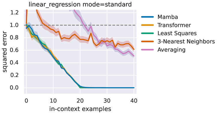
(a) Linear Regression

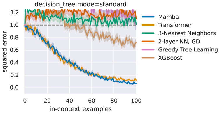
(b) Decision Tree

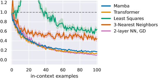
(c) ReLU Neural Network

Figure 5: Mamba compares with transformers when trained and tested on the same simple regression task distributions.

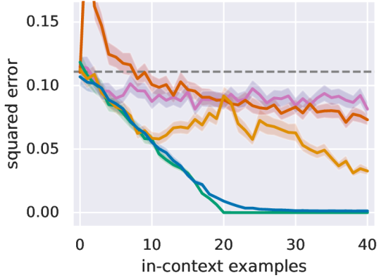
(a) x-scale 0.333

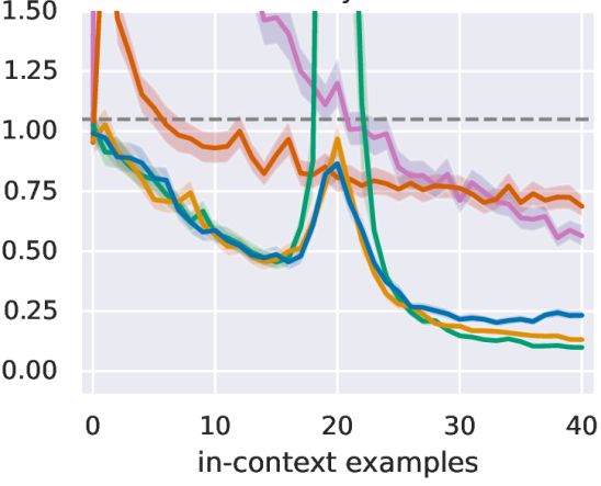
(b) Noisy LR

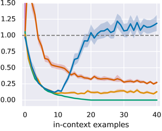
(c) Skewed LR

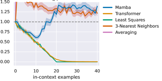
(d) Random Quadrants

Figure 6: OOD Distribution tests for Mamba and Transformer trained on (non-skewed) linear regression data

A.2.6 ICL learning curves

In our experimental setup, we employed a total of 40 in-context examples and evaluated the model on 30 distinct query examples. Each query example was assessed through an independent forward pass, resulting in 30 separate predictions made by processing a batch of 41 samples (in-context plus query) within the model, a method analogous to that described by Garg et al. (2022). Throughout these forward passes, we captured the feature activations (embeddings) from the intermediate layers for analysis. We carried out this analysis for 64 different tasks with 70 total examples each (40 in-context and 30 query examples).

We now describe the probing strategy in detail. Consider the input prompt $(x_{1},y_{1},x_{2},y_{2},...,x_{k},y_{k},x_{k+1})$, let $z_{l,i}$ be the model internal representation of the input token $x_{i}$ at layer $l$, and denote by $\hat{y}_{i}=g(z_{L,i})$ the model prediction for $x_{i}$, where $g$ is the decoder and $L$ is the total number of layers. For each layer $l$ we first obtain intermediate scalar predictions $\tilde{y}_{l,i}=g(z_{l,i})$. Since $g$ is not meant to be used on intermediate representations, we adjust the prediction on the query point $x_{k+1}$ by computing $\hat{y}_{l,k+1}=a_{l}g(z_{l,k+1})+b_{l}$, where the scalar scale and shift parameters $a_{l}$ and $b_{l}$ are obtained by least squares on the input-output pairs $(\tilde{y}_{l,k-n+1},y_{k-n+1}),(\tilde{y}_{l,k},y_{k})$, with $n=10$ and $k=40$. We can then measure the squared error $(\hat{y}_{l,k+1}-y_{k+1})^{2}$ between the intermediate predictions and the target.

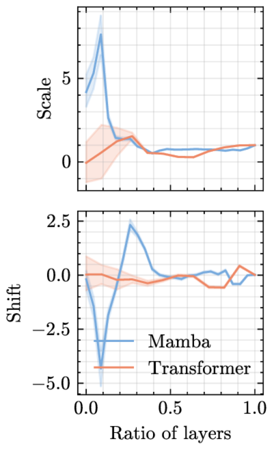
(a) Skewed LR

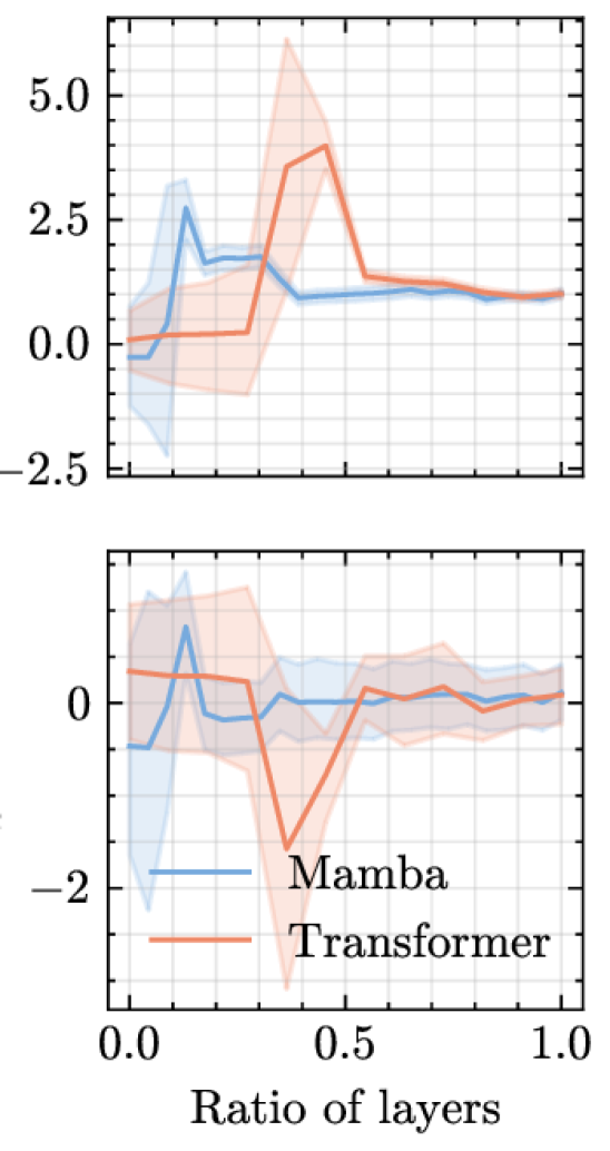
(b) ReLU NN

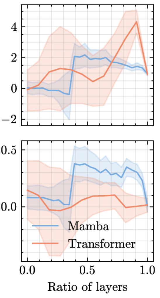
(c) Decision Tree

Figure 8: Estimated scalar scale and shift by the linear probing model used in Section 2.2.

As mentioned above, for constructing the linear model, we selectively used the representation from the in-context examples ranging from the 30th to the 40th. This selective usage was due to the observation that the model’s initial predictions are suboptimal, as evidenced by the performance comparison in Figure 1. By focusing on later samples, we aim to derive a more accurate linear model based on the embeddings corresponding to more refined predictions.

The scale and shift were estimated for each layer and are reported in Figure 8. We note that for skewed linear regression and ReLU neural networks the value for scale approaches 1, and the one for shift approaches 0 relatively quickly.

A.3 ICL for NLP tasks

Table 1: Complete results of the ICL benchmark by Hendel et al. (2023) for all tasks and models. Regular denotes the ICL setting as described in Section 3 and baseline refers to zero-shot performance (i.e. a query without any examples).

		Method	Baseline	Regular
Model	Task type	Task name
GPT-J 6B	Algorithmic	List first	0.30	0.98
		List last	0.24	1.00
		Next letter	0.16	0.86
		Prev letter	0.10	0.42
		To lower	0.00	1.00
		To upper	0.00	1.00
	Knowledge	Country capital	0.19	0.80
		Location continent	0.03	0.70
		Location religion	0.09	0.78
		Person language	0.02	0.82
	Linguistic	Antonyms	0.43	0.78
		Plural singular	0.08	0.98
		Present simple gerund	0.00	0.98
		Present simple past simple	0.02	0.96
	Translation	En es	0.14	0.56
		En fr	0.16	0.54
		Es en	0.06	0.74
		Fr en	0.13	0.76
LLaMA 13B	Algorithmic	List first	0.77	1.00
		List last	0.07	0.92
		Next letter	0.31	0.94
		Prev letter	0.05	0.50
		To lower	0.00	1.00
		To upper	0.00	1.00
	Knowledge	Country capital	0.17	0.86
		Location continent	0.01	0.80
		Location religion	0.10	0.84
		Person language	0.02	0.88
	Linguistic	Antonyms	0.19	0.80
		Plural singular	0.24	0.88
		Present simple gerund	0.00	0.96
		Present simple past simple	0.01	0.98
	Translation	En es	0.05	0.82
		En fr	0.15	0.84
		Es en	0.29	0.88
		Fr en	0.25	0.72
LLaMA 30B	Algorithmic	List first	0.96	1.00
		List last	0.02	0.96
		Next letter	0.30	0.96
		Prev letter	0.02	0.80
		To lower	0.00	1.00
		To upper	0.00	1.00
	Knowledge	Country capital	0.27	0.88
		Location continent	0.01	0.86
		Location religion	0.05	0.88
		Person language	0.01	0.90
	Linguistic	Antonyms	0.37	0.82
		Plural singular	0.21	0.90
		Present simple gerund	0.00	0.98
		Present simple past simple	0.02	1.00
	Translation	En es	0.07	0.78
		En fr	0.10	0.86
		Es en	0.24	0.88
		Fr en	0.20	0.78
LLaMA 7B	Algorithmic	List first	0.87	1.00
		List last	0.03	1.00
		Next letter	0.03	0.88
		Prev letter	0.04	0.58
		To lower	0.00	1.00
		To upper	0.00	1.00
	Knowledge	Country capital	0.28	0.86
		Location continent	0.02	0.72
		Location religion	0.12	0.94
		Person language	0.02	0.78
	Linguistic	Antonyms	0.33	0.76
		Plural singular	0.15	0.88
		Present simple gerund	0.00	0.90
		Present simple past simple	0.02	0.92
	Translation	En es	0.07	0.76
		En fr	0.04	0.88
		Es en	0.21	0.92
		Fr en	0.15	0.70
Mamba 0.13B	Algorithmic	List first	0.66	0.92
		List last	0.02	0.92
		Next letter	0.16	0.76
		Prev letter	0.02	0.02
		To lower	0.00	1.00
		To upper	0.00	1.00
	Knowledge	Country capital	0.08	0.20
		Location continent	0.00	0.55
		Location religion	0.02	0.67
		Person language	0.02	0.48
	Linguistic	Antonyms	0.19	0.30
		Plural singular	0.06	0.44
		Present simple gerund	0.00	0.67
		Present simple past simple	0.02	0.69
	Translation	En es	0.06	0.25
		En fr	0.14	0.37
		Es en	0.09	0.21
		Fr en	0.08	0.25
Mamba 0.37B	Algorithmic	List first	0.09	1.00
		List last	0.02	0.95
		Next letter	0.04	0.87
		Prev letter	0.09	0.12
		To lower	0.00	1.00
		To upper	0.00	1.00
	Knowledge	Country capital	0.10	0.53
		Location continent	0.01	0.69
		Location religion	0.02	0.59
		Person language	0.02	0.75
	Linguistic	Antonyms	0.29	0.67
		Plural singular	0.04	0.74
		Present simple gerund	0.00	0.86
		Present simple past simple	0.00	0.81
	Translation	En es	0.07	0.45
		En fr	0.13	0.48
		Es en	0.06	0.79
		Fr en	0.07	0.74
Mamba 0.79B	Algorithmic	List first	0.76	1.00
		List last	0.03	0.95
		Next letter	0.09	0.88
		Prev letter	0.04	0.34
		To lower	0.00	1.00
		To upper	0.00	1.00
	Knowledge	Country capital	0.18	0.71
		Location continent	0.03	0.73
		Location religion	0.12	0.73
		Person language	0.01	0.79
	Linguistic	Antonyms	0.39	0.76
		Plural singular	0.12	0.86
		Present simple gerund	0.00	0.91
		Present simple past simple	0.00	0.85
	Translation	En es	0.20	0.56
		En fr	0.16	0.58
		Es en	0.18	0.78
		Fr en	0.13	0.75
Mamba 1.40B	Algorithmic	List first	0.68	1.00
		List last	0.03	0.93
		Next letter	0.07	0.81
		Prev letter	0.09	0.34
		To lower	0.00	1.00
		To upper	0.00	1.00
	Knowledge	Country capital	0.20	0.71
		Location continent	0.02	0.76
		Location religion	0.04	0.83
		Person language	0.00	0.83
	Linguistic	Antonyms	0.30	0.77
		Plural singular	0.11	0.86
		Present simple gerund	0.00	0.91
		Present simple past simple	0.00	0.92
	Translation	En es	0.17	0.73
		En fr	0.24	0.67
		Es en	0.07	0.83
		Fr en	0.11	0.78
Mamba 2.80B	Algorithmic	List first	0.69	1.00
		List last	0.13	0.97
		Next letter	0.05	0.93
		Prev letter	0.00	0.39
		To lower	0.00	1.00
		To upper	0.00	1.00
	Knowledge	Country capital	0.20	0.75
		Location continent	0.02	0.82
		Location religion	0.07	0.82
		Person language	0.00	0.86
	Linguistic	Antonyms	0.25	0.77
		Plural singular	0.17	0.90
		Present simple gerund	0.00	0.95
		Present simple past simple	0.00	0.93
	Translation	En es	0.11	0.78
		En fr	0.12	0.69
		Es en	0.05	0.83
		Fr en	0.11	0.78
Mamba 2.80B (SP)	Algorithmic	List first	0.84	1.00
		List last	0.07	0.92
		Next letter	0.12	0.82
		Prev letter	0.02	0.22
		To lower	0.00	1.00
		To upper	0.00	1.00
	Knowledge	Country capital	0.31	0.81
		Location continent	0.04	0.86
		Location religion	0.07	0.87
		Person language	0.03	0.83
	Linguistic	Antonyms	0.34	0.78
		Plural singular	0.11	0.89
		Present simple gerund	0.00	0.90
		Present simple past simple	0.02	0.92
	Translation	En es	0.09	0.73
		En fr	0.09	0.59
		Es en	0.12	0.81
		Fr en	0.11	0.80
Pythia 12B	Algorithmic	List first	0.53	0.96
		List last	0.09	1.00
		Next letter	0.15	0.76
		Prev letter	0.00	0.42
		To lower	0.02	1.00
		To upper	0.00	1.00
	Knowledge	Country capital	0.19	0.82
		Location continent	0.01	0.80
		Location religion	0.07	0.78
		Person language	0.01	0.86
	Linguistic	Antonyms	0.34	0.74
		Plural singular	0.18	0.84
		Present simple gerund	0.00	0.96
		Present simple past simple	0.01	0.94
	Translation	En es	0.10	0.72
		En fr	0.16	0.54
		Es en	0.05	0.80
		Fr en	0.14	0.80
Pythia 2.8B	Algorithmic	List first	0.69	1.00
		List last	0.06	1.00
		Next letter	0.42	0.90
		Prev letter	0.01	0.48
		To lower	0.00	1.00
		To upper	0.00	1.00
	Knowledge	Country capital	0.18	0.76
		Location continent	0.01	0.72
		Location religion	0.08	0.82
		Person language	0.00	0.82
	Linguistic	Antonyms	0.37	0.76
		Plural singular	0.13	0.78
		Present simple gerund	0.00	0.96
		Present simple past simple	0.03	0.92
	Translation	En es	0.10	0.76
		En fr	0.16	0.60
		Es en	0.08	0.82
		Fr en	0.10	0.82
Pythia 6.9B	Algorithmic	List first	0.43	0.98
		List last	0.08	0.98
		Next letter	0.01	0.86
		Prev letter	0.04	0.32
		To lower	0.00	1.00
		To upper	0.00	1.00
	Knowledge	Country capital	0.21	0.82
		Location continent	0.01	0.78
		Location religion	0.10	0.80
		Person language	0.01	0.80
	Linguistic	Antonyms	0.33	0.74
		Plural singular	0.14	0.88
		Present simple gerund	0.00	0.94
		Present simple past simple	0.02	0.96
	Translation	En es	0.11	0.70
		En fr	0.21	0.60
		Es en	0.06	0.82
		Fr en	0.14	0.74
RWKV 0.169B	Algorithmic	List first	0.48	0.46
		List last	0.10	0.19
		Next letter	0.12	0.27
		Prev letter	0.04	0.03
		To lower	0.00	0.57
		To upper	0.00	0.86
	Knowledge	Country capital	0.14	0.09
		Location continent	0.00	0.67
		Location religion	0.03	0.62
		Person language	0.00	0.33
	Linguistic	Antonyms	0.09	0.06
		Plural singular	0.16	0.22
		Present simple gerund	0.00	0.21
		Present simple past simple	0.01	0.14
	Translation	En es	0.14	0.14
		En fr	0.11	0.25
		Es en	0.02	0.09
		Fr en	0.14	0.09
RWKV 0.43B	Algorithmic	List first	0.40	0.73
		List last	0.17	0.48
		Next letter	0.07	0.64
		Prev letter	0.00	0.02
		To lower	0.00	1.00
		To upper	0.00	1.00
	Knowledge	Country capital	0.14	0.34
		Location continent	0.00	0.58
		Location religion	0.10	0.69
		Person language	0.01	0.59
	Linguistic	Antonyms	0.10	0.58
		Plural singular	0.13	0.21
		Present simple gerund	0.00	0.53
		Present simple past simple	0.01	0.59
	Translation	En es	0.04	0.38
		En fr	0.03	0.31
		Es en	0.10	0.58
		Fr en	0.08	0.52
RWKV 1.5B	Algorithmic	List first	0.51	0.97
		List last	0.26	0.78
		Next letter	0.22	0.78
		Prev letter	0.00	0.04
		To lower	0.00	1.00
		To upper	0.00	1.00
	Knowledge	Country capital	0.12	0.40
		Location continent	0.00	0.56
		Location religion	0.02	0.70
		Person language	0.00	0.76
	Linguistic	Antonyms	0.31	0.68
		Plural singular	0.07	0.70
		Present simple gerund	0.00	0.70
		Present simple past simple	0.01	0.79
	Translation	En es	0.21	0.63
		En fr	0.14	0.57
		Es en	0.15	0.78
		Fr en	0.08	0.77

References

- Ahn et al. (2023) Kwangjun Ahn, Xiang Cheng, Hadi Daneshmand, and Suvrit Sra. Transformers learn to implement preconditioned gradient descent for in-context learning. arXiv preprint arXiv:2306.00297, 2023.
- Akyürek et al. (2023) Ekin Akyürek, Dale Schuurmans, Jacob Andreas, Tengyu Ma, and Denny Zhou. What learning algorithm is in-context learning? Investigations with linear models. In The Eleventh International Conference on Learning Representations, 2023.
- Akyürek et al. (2024) Ekin Akyürek, Bailin Wang, Yoon Kim, and Jacob Andreas. In-context language learning: Architectures and Algorithms. arXiv preprint arXiv:2401.12973, 2024.
- Bai et al. (2023) Yu Bai, Fan Chen, Huan Wang, Caiming Xiong, and Song Mei. Transformers as Statisticians: Provable in-context learning with in-context algorithm selection. Advances in neural information processing systems, 2023.
- Biderman et al. (2023) Stella Biderman, Hailey Schoelkopf, Quentin Gregory Anthony, Herbie Bradley, Kyle O’Brien, Eric Hallahan, Mohammad Aflah Khan, Shivanshu Purohit, USVSN Sai Prashanth, Edward Raff, et al. Pythia: A suite for analyzing large language models across training and scaling. In International Conference on Machine Learning, pp. 2397–2430. PMLR, 2023.
- Brown et al. (2020) Tom Brown, Benjamin Mann, Nick Ryder, Melanie Subbiah, Jared D Kaplan, Prafulla Dhariwal, Arvind Neelakantan, Pranav Shyam, Girish Sastry, Amanda Askell, et al. Language models are few-shot learners. Advances in neural information processing systems, 33:1877–1901, 2020.
- Chen & Guestrin (2016) Tianqi Chen and Carlos Guestrin. Xgboost: A scalable tree boosting system. Proceedings of the 22nd ACM SIGKDD International Conference on Knowledge Discovery and Data Mining, 2016.
- Gao et al. (2020) Leo Gao, Stella Biderman, Sid Black, Laurence Golding, Travis Hoppe, Charles Foster, Jason Phang, Horace He, Anish Thite, Noa Nabeshima, et al. The Pile: An 800GB dataset of diverse text for language modeling. arXiv preprint arXiv:2101.00027, 2020.
- Garg et al. (2022) Shivam Garg, Dimitris Tsipras, Percy S Liang, and Gregory Valiant. What can transformers learn in-context? A case study of simple function classes. Advances in Neural Information Processing Systems, 35:30583–30598, 2022.
- Geva et al. (2021) Mor Geva, Roei Schuster, Jonathan Berant, and Omer Levy. Transformer feed-forward layers are key-value memories. In Proceedings of the 2021 Conference on Empirical Methods in Natural Language Processing, pp. 5484–5495, 2021.
- Gu & Dao (2023) Albert Gu and Tri Dao. Mamba: Linear-time sequence modeling with selective state spaces. arXiv preprint arXiv:2312.00752, 2023.
- Gu et al. (2021a) Albert Gu, Karan Goel, and Christopher Re. Efficiently modeling long sequences with structured state spaces. In International Conference on Learning Representations, 2021a.
- Gu et al. (2021b) Albert Gu, Isys Johnson, Karan Goel, Khaled Saab, Tri Dao, Atri Rudra, and Christopher Ré. Combining recurrent, convolutional, and continuous-time models with linear state space layers. Advances in neural information processing systems, 34:572–585, 2021b.
- Hendel et al. (2023) Roee Hendel, Mor Geva, and Amir Globerson. In-context learning creates task vectors. In Findings of the Association for Computational Linguistics: EMNLP 2023, pp. 9318–9333, 2023.
- Hospedales et al. (2021) Timothy Hospedales, Antreas Antoniou, Paul Micaelli, and Amos Storkey. Meta-learning in neural networks: A survey. IEEE transactions on pattern analysis and machine intelligence, 44(9):5149–5169, 2021.
- Kalman (1960) Rudolph Emil Kalman. A new approach to linear filtering and prediction problems. Transactions of the ASME–Journal of Basic Engineering, 82(Series D):35–45, 1960.
- Lee et al. (2023) Ivan Lee, Nan Jiang, and Taylor Berg-Kirkpatrick. Exploring the relationship between model architecture and in-context learning ability. arXiv preprint arXiv:2310.08049, 2023.
- Ma et al. (2024) Jun Ma, Feifei Li, and Bo Wang. U-Mamba: Enhancing long-range dependency for biomedical image segmentation. arXiv preprint arXiv:2401.04722, 2024.
- Müller et al. (2021) Samuel Müller, Noah Hollmann, Sebastian Pineda Arango, Josif Grabocka, and Frank Hutter. Transformers can do bayesian inference. In International Conference on Learning Representations, 2021.
- Peng et al. (2023) Bo Peng, Eric Alcaide, Quentin Anthony, Alon Albalak, Samuel Arcadinho, Huanqi Cao, Xin Cheng, Michael Chung, Matteo Grella, Kranthi Kiran GV, et al. RWKV: Reinventing RNNs for the Transformer Era. arXiv preprint arXiv:2305.13048, 2023.
- Press et al. (2021) Ofir Press, Noah Smith, and Mike Lewis. Train short, test long: Attention with linear biases enables input length extrapolation. In International Conference on Learning Representations, 2021.
- Radford et al. (2019) A. Radford, J. Wu, R. Child, D. Luan, D. Amodei, and I. Sutskever. Language models are unsupervised multitask learners. OpenAI blog, 1(8):9, 2019.
- Shen et al. (2023) Lingfeng Shen, Aayush Mishra, and Daniel Khashabi. Do pretrained transformers really learn in-context by gradient descent? arXiv preprint arXiv:2310.08540, 2023.
- Tay et al. (2021) Yi Tay, Mostafa Dehghani, Samira Abnar, Yikang Shen, Dara Bahri, Philip Pham, Jinfeng Rao, Liu Yang, Sebastian Ruder, and Donald Metzler. Long Range Arena: A Benchmark for Efficient Transformers. In International Conference on Learning Representations, 2021.
- Touvron et al. (2023) Hugo Touvron, Thibaut Lavril, Gautier Izacard, Xavier Martinet, Marie-Anne Lachaux, Timothée Lacroix, Baptiste Rozière, Naman Goyal, Eric Hambro, Faisal Azhar, et al. Llama: Open and efficient foundation language models. arXiv preprint arXiv:2302.13971, 2023.
- Vaswani et al. (2017) Ashish Vaswani, Noam Shazeer, Niki Parmar, Jakob Uszkoreit, Llion Jones, Aidan N Gomez, Ł ukasz Kaiser, and Illia Polosukhin. Attention is all you need. In Advances in Neural Information Processing Systems, volume 30, 2017.
- Von Oswald et al. (2023) Johannes Von Oswald, Eyvind Niklasson, Ettore Randazzo, João Sacramento, Alexander Mordvintsev, Andrey Zhmoginov, and Max Vladymyrov. Transformers learn in-context by gradient descent. In International Conference on Machine Learning, pp. 35151–35174. PMLR, 2023.
- Wang & Komatsuzaki (2021) Ben Wang and Aran Komatsuzaki. GPT-J-6B: A 6 Billion Parameter Autoregressive Language Model. https://github.com/kingoflolz/mesh-transformer-jax, May 2021.
- Zhu et al. (2024) Lianghui Zhu, Bencheng Liao, Qian Zhang, Xinlong Wang, Wenyu Liu, and Xinggang Wang. Vision Mamba: Efficient visual representation learning with bidirectional state space model. arXiv preprint arXiv:2401.09417, 2024.