Holonomy operator for spin connection and spatial scalar curvature operator in loop quantum gravity

Abstract

In this article we propose a new construction of the spatial scalar curvature operator in (1+3)-dimensional LQG based on the twisted geometry. The starting point of the construction is to express the holonomy of the spin connection on a graph in terms of the twisted geometry variables, and we check that this expression reproduces the spin connection in terms of triads in a certain continuum limit. The spatial scalar curvature in terms of twisted geometry is obtained by considering the composition of the holonomy of the spin connection on the loops. With the twisted geometry parametrization of the holonomy-flux phase space, we further express the holonomy of the spin connection and the spatial scalar curvature on a graph in terms of fluxes. Finally, they are promoted as well-defined operators by replacing the fluxes with ordered flux operators.

1 Introduction

Loop quantum gravity (LQG) is a promising approach to non-perturbative and background independent quantum gravity [1, 2, 3, 4]. This theory starts from the Hamiltonian formulation of (1+3)-dimensional general relativity (GR), which is formulated as a Yang-Mills gauge theory, with the Ashtekar-Barbero connection and desitized triads on 3-dimensional spatial slice being the conjugate pairs and Gaussian constraint generating the gauge transformations. The quantum states of this theory are spin-network states, which provide the basic building blocks of the discrete quantum geometry. Also, this quantization framework is extended to all dimensional GR, and it leads to similar kinematical structures which describe the discrete quantum geometry in arbitrary spacetime [5, 6, 7, 8]. Based on classical deparametrized models of gravity, such as gravity coupled to dust fields or scalar fields, the reduced phase space quantization is proposed for LQG [9, 10, 11, 12, 13]. With the dynamical constraints being solved classically and the coupled dust fields or scalar fields being used to parametrize the spacetime coordinates, the reduced phase space quantization has a true physical Hamiltonian instead of a Hamiltonian constraint, and the gauge invariant Hilbert space with respect to the Gaussian constraint in LQG becomes the physical Hilbert space of Dirac observables. Correspondingly, the quantum dynamics is governed by the entire LQG physical Hamiltonian defined on the physical Hilbert space. One of the popular Hamiltonians is given by the Giesel-Thiemann construction [14, 1, 9], where the Hamiltonian constraint is separated into Euclidean and Lorentzian terms. Thiemann’s method is employed to quantize the Lorentzian term in relation to the extrinsic curvature operators [1]. It has been shown that the semiclassical limit of the theory based on the reduced phase space coherent state path integral formulation reproduces classical reduced phase space equation of motions (EOMs) of gravity [15, 16, 17]. Thus, it is semiclassically consistent.

There is another proposal for the Hamiltonian by Alesci-Assanioussi-Lewandowski-Makinen (AALM) [18, 19], which replaces the relatively complicated form of the Lorentzian term with the spatial scalar curvature on the 3-dimensional spatial slice. The spatial scalar curvature itself is a geometric observable characterizing the geometry of the spatial manifold. Additionally, similar formulations are widely used in symmetry-reduced models inspired by LQG, such as standard loop quantum cosmology (LQC) and loop quantum black hole models, leading to singularity resolution and big bounce [20, 21, 22, 23, 24, 25, 26, 27, 28, 29, 30, 31, 32, 33, 34, 35, 36, 37, 38, 39]. Consequently, a scalar curvature operator will play an important role in deriving symmetry-reduced models from the first principle of full LQG. Moreover, this proposal is also considered in all dimensional LQG to avoid the problem that the Euclidean term of Hamiltonian constraint cannot capture the degrees of freedom of the intrinsic curvature [40].

The proposed operator representing the spatial scalar curvature is quantized with Regge calculus techniques on a cellular decomposition of the spatial manifold [41, 42]. However, contrary to the Giesel-Thiemann construction, the continuum limit of such an operator is not straightforward and it is not compatible with the Euclidean part of the Hamiltonian constraint on a fixed graph. The conflict is related to the fact that the Regge calculus relies on a cellular decomposition dual to the graph, and to the fact that the holonomy-flux variables on a fixed graph correspond to twisted geometry instead of Regge geometry [43, 44, 45]. To avoid such a problem, a new quantization of the scalar curvature operator on a cubic graph with regularization of the densitized triad and its covariant derivatives is proposed [46, 47]. However, the operator is only defined on a cubical graph with a relatively complicated formula and has no intuitive discrete geometric interpretation.

The issues encountered in previous works inspire us to establish the spatial scalar curvature operator based on the twisted geometry instead of the Regge geometry. More explicitly, the twisted geometry provides a parametrization of the holonomy-flux phase space, hence the discrete geometry captured by the holonomy-flux variables on a fixed graph is interpreted by the twisted geometry instead of the Regge geometry [43, 44, 45, 48]. In fact, the space of Regge geometry, which is given by imposing the shape-matching condition of the 2-face in the twisted geometry space, is a subspace of the twisted geometry space on the graph dual to a cellular decomposition. Moreover, the Hilbert space spanned by spin network states on the graph is given by quantizing the corresponding holonomy-flux phase space. Therefore, it is reasonable to construct the spatial scalar curvature operator based on the twisted geometry instead of the Regge geometry. This ensures that the corresponding spatial scalar curvature operator acting on the spin network states could represent the correct quantum degrees of freedom of the discrete geometry.

In this paper, we propose a new scalar curvature operator based on the holonomy operators of spin connections. First, we establish the holonomy of the spin connection based on the twisted geometry variables. Correspondingly, the 3-D discrete scalar curvature on a closed graph can be established based on the holonomy of spin connections. We also check that the holonomy of the spin connection and the corresponding spatial discrete scalar curvature on the cubic graph reproduce the continuum spin connection and the 3-D curvature in the continuum limit in a certain coordinate system. Then, note the twisted geometric parameterization of the holonomy-flux phase space, the holonomy of the spin connection and the spatial discrete scalar curvature can be expressed by the fluxes. Finally, up to the operator ordering, they can be promoted as operators by simply replacing the classical fluxes by flux operators.

This paper is organized as follows. In the following section 2 we will review the kinematical structure and the existing treatment of the Hamiltonian constraint in LQG. In particular, this section also serves to introduce the twisted geometry parametrization of the holonomy-flux phase space on a fixed graph. In section 3 we introduce the construction of the holonomy of the spin connection and the spatial scalar curvature on a graph in terms of the twisted geometry variables, and check that these expressions reproduce correct continuum limits for the cubic graph. Then, in section 4, we propose the quantization of these expressions. Finally, in section 5 we summarize and discuss the results with an outlook on the possible next steps of future research.

2 Elements of LQG

2.1 The basic structures

The (1+3)-dimensional Lorentzian LQG is constructed by canonically quantizing GR based on the Yang-Mills phase space with the non-vanishing Poisson bracket[2, 4]

$$\{A_{a}^{i}(x),E^{b}_{j}(y)\}=\kappa\beta\delta_{a}^{b}\delta^{i}_{j}\delta^{(3)}(x-y),$$ (1)

where the configuration and momentum variables are the $su(2)$-valued connection field $A_{a}^{i}$ and the densitized triad field $E^{b}_{j}$ respectively on a 3-dimensional spatial manifold $\Sigma$, $\kappa=8\pi G$ with the gravitational constant $G$, and $\beta$ represent the Babero-Immirze parameter. Here we use $i,j,k,...$ for the internal $su(2)$ index and $a,b,c,...$ for the spatial index. Let $q_{ab}=e_{a}^{i}e_{bi}$ be the spatial metric on $\Sigma$. The densitized triad is related to the triad $e_{i}^{a}$ by $E^{a}_{i}=\sqrt{\det(q)}e^{a}_{i}$, where $\det(q)$ denotes the determinant of $q_{ab}$. The connection can be expressed as $A_{a}^{i}=\Gamma_{a}^{i}+\beta K_{a}^{i}$, where $\Gamma_{a}^{i}$ is the Levi-Civita connection of $e_{a}^{i}$, which is given by [1]

$$\Gamma_{a}^{i}=\frac{1}{2}\epsilon^{ijk}e_{k}^{b}(\partial_{b}e_{a}^{j}-\partial_{a}e_{b}^{j}+e^{c}_{j}e_{al}\partial_{b}e^{l}_{c}).$$ (2)

$K_{a}^{i}$ is related to the extrinsic curvature $K_{ab}$ by $K_{a}^{i}=K_{ab}e^{b}_{j}\delta^{ji}$. The Gaussian constraint which generates gauge transformation is given by

$$\mathcal{G}:=\partial_{a}E^{ai}+A_{aj}E^{a}_{k}\epsilon^{ijk}\approx 0.$$ (3)

Again, the dynamics of LQG can be defined by the physical Hamiltonian which is introduced by the classical deparametrization of GR. In the deparametrization models with certain dust fields, the diffeomorphism and Hamiltonian constraints are solved classically and the dust reference frame provides the physical space-time coordinates, so that the theory is described in terms of Dirac observables [11][12][13]. Then, the physical time evolution is generated by the physical Hamiltonian with respect to the dust fields. More explicitly, the resulting physical Hamiltonian $\mathbf{H}$ can be written as $\mathbf{H}=\int_{\Sigma}dx^{3}h$, where $h=h(\mathcal{C},\mathcal{C}_{a})$ takes different formulations for different deparametrization models. The diffeomorphism constraint $\mathcal{C}_{a}$ and the Hamiltonian constraint $\mathcal{C}$ are given by

$$\mathcal{C}_{a}:=E^{b}_{i}F^{i}_{ab},$$ (4)

and

$$\mathcal{C}:=\frac{E^{a}_{i}E^{b}_{j}}{\sqrt{|\det{(E)}|}}({\epsilon^{ij}}_{k}F^{k}_{ab}-2(1+\beta^{2})K^{i}_{[a}K^{j}_{b]}),$$ (5)

respectively, where $F_{ab}^{i}=\partial_{a}A_{b}^{i}-\partial_{b}A_{a}^{i}+\epsilon_{ijk}A_{a}^{j}A_{b}^{k}$ is the curvature of $A_{a}^{i}$. Equivalently, the Hamiltonian can also be given by [18, 19]

$$\mathcal{C}:=-\frac{1}{\beta^{2}}\frac{E^{a}_{i}E^{b}_{j}}{\sqrt{|\det{(E)}|}}{\epsilon^{ij}}_{k}F^{k}_{ab}-(1+\frac{1}{\beta^{2}})\sqrt{|\det{(E)}|}R\approx 0,$$ (6)

where $\sqrt{|\det{(E)}|}R:=-\sqrt{|\det{(E)}|}R_{ab}^{j}\epsilon_{jkl}e^{ak}e^{bl}$ is the densitized scalar curvature of the spatial metric $q_{ab}$, with $R_{ab}^{j}:=2\partial_{[a}\Gamma_{b]}^{j}+\epsilon^{j}_{\ kl}\Gamma_{a}^{k}\Gamma^{l}_{b}$ [1].

The loop quantization of the $SU(2)$ connection formulation of GR leads to a kinematical Hilbert space $\mathcal{H}$, which can be regarded as a union of the Hilbert spaces $\mathcal{H}_{\gamma}=L^{2}((SU(2))^{|E(\gamma)|},d\mu_{\text{Haar}}^{|E(\gamma)|})$ on all possible graphs $\gamma$, where $|E(\gamma)|$ denotes the number of independent edges of $\gamma$ and $d\mu_{\text{Haar}}$ denotes the product of the Haar measure on $SU(2)$. In this sense, on each given $\gamma$ there is a discrete phase space $(T^{\ast}SU(2))^{|E(\gamma)|}$, which is coordinatized by the basic discrete variables—holonomies and fluxes. The holonomy of $A_{a}^{i}$ along an edge $e\in\gamma$ is defined by

$$h_{e}[A]:=\mathcal{P}\exp(\int_{e}A)=1+\sum_{n=1}^{\infty}\int_{0}^{1}dt_{n}\int_{0}^{t_{n}}dt_{n-1}...\int_{0}^{t_{2}}dt_{1}A(t_{1})...A(t_{n}),$$ (7)

where $A(t)=A_{a}^{i}(t)\dot{e}^{a}(t)\tau_{i}$, and $\tau_{i}=-\frac{\mathbf{i}}{2}\sigma_{i}$ with $\sigma_{i}$ being the Pauli matrices. There are two versions for the gauge covariant flux of $E^{b}_{j}$ through the 2-face dual to edge $e\in\gamma$ [49, 50]. The flux $F^{i}_{e}$ (or denoted by $F^{i}(e)$) in the perspective of source point of $e$ is defined by

$$F^{i}_{e}:=\frac{2}{\beta}\text{tr}\left(\tau^{i}\int_{S_{e}}\epsilon_{abc}h(\rho^{s}_{e}(\sigma))E^{cj}(\sigma)\tau_{j}h(\rho^{s}_{e}(\sigma)^{-1})\right),$$ (8)

where $S_{e}$ is the 2-face in the dual lattice $\gamma^{\ast}$ of $\gamma$, $\rho^{s}(\sigma):[0,1]\rightarrow\Sigma$ is a path connecting the source point $s_{e}\in e$ to $\sigma\in S_{e}$ such that $\rho_{e}^{s}(\sigma):[0,\frac{1}{2}]\rightarrow e$ and $\rho_{e}^{s}(\sigma):[\frac{1}{2},1]\rightarrow S_{e}$. Similarly, the corresponding flux $\tilde{F}^{i}_{e}$ (or denoted by $\tilde{F}^{i}(e)$) in the perspective of target point of $e$ is defined by

$$\tilde{F}^{i}_{e}:=-\frac{2}{\beta}\text{tr}\left(\tau^{i}\int_{S_{e}}\epsilon_{abc}h(\rho^{t}_{e}(\sigma))E^{cj}(\sigma)\tau_{j}h(\rho^{t}_{e}(\sigma)^{-1})\right),$$ (9)

where $\rho^{t}(\sigma):[0,1]\rightarrow\Sigma$ is a path connecting the target point $t_{e}\in e$ to $\sigma\in S_{e}$ such that $\rho_{e}^{t}(\sigma):[0,\frac{1}{2}]\rightarrow e$ and $\rho_{e}^{t}(\sigma):[\frac{1}{2},1]\rightarrow S_{e}$. It is easy to see that one has the relation

$$\tilde{F}^{i}_{e}\tau_{i}=-h_{e}^{-1}{F}^{i}_{e}\tau_{i}h_{e}.$$ (10)

The non-vanishing Poisson brackets among the holonomy and fluxes read

$$\{{{h}}_{e}[{A}],{{F}}^{i}_{e^{\prime}}\}=-\delta_{e,e^{\prime}}{\kappa}\tau^{i}{{h}}_{e}[{A}],\quad\{{{h}}_{e}[{A}],\tilde{{F}}^{i}_{e^{\prime}}\}=\delta_{e,e^{\prime}}{\kappa}{{h}}_{e}[{A}]\tau^{i},$$ (11)

$$\{{{F}}^{i}_{e},{{F}}^{j}_{e^{\prime}}\}=-\delta_{e,e^{\prime}}{\kappa}{\epsilon^{ij}}_{k}{{F}}^{k}_{e^{\prime}},\quad\{\tilde{{F}}^{i}_{e},\tilde{{F}}^{j}_{e^{\prime}}\}=-\delta_{e,e^{\prime}}{\kappa}{\epsilon^{ij}}_{k}\tilde{{F}}^{k}_{e^{\prime}}.$$

The basic operators in $\mathcal{H}_{\gamma}$ is given by promoting the basic discrete variables as operators. The resulting holonomy and flux operators act on cylindrical functions $f_{\gamma}(A)=f_{\gamma}(h_{e_{1}}[A],...,h_{e_{|E(\gamma)|}}[A])$ in $\mathcal{H}_{\gamma}$ as

$$\hat{h}_{e}[A]f_{\gamma}(A)=h_{e}[A]f_{\gamma}(A),$$ (12)

$$\hat{F}^{i}_{e}f_{\gamma}(h_{e_{1}}[A],...,h_{e}[A],...,h_{e_{|E(\gamma)|}}[A]=\mathbf{i}\kappa\hbar\frac{d}{d\lambda}f_{\gamma}\left.\left(h_{e_{1}}[A],...,e^{\lambda\tau^{i}}h_{e}[A],...,h_{e_{|E(\gamma)|}}[A]\right)\right|_{\lambda=0},$$ (13)

$$\hat{\tilde{F}}^{i}_{e}f_{\gamma}(h_{e_{1}}[A],...,h_{e}[A],...,h_{e_{|E(\gamma)|}}[A]=-\mathbf{i}\kappa\hbar\frac{d}{d\lambda}f_{\gamma}\left.\left(h_{e_{1}}[A],...,h_{e}[A]e^{\lambda\tau^{i}},...,h_{e_{|E(\gamma)|}}[A]\right)\right|_{\lambda=0}.$$ (14)

Two spatial geometric operators in $H_{\gamma}$ are worth being mentioned here. The first one is the oriented area operator defined as $\beta\hat{F}^{i}_{e}$ (or $\beta\hat{\tilde{F}}^{i}_{e}$), whose module length $|\beta\hat{F}_{e}|:=\sqrt{\beta^{2}\hat{F}^{i}(e)\hat{F}_{i}(e)}$ represents the area of the 2-face dual to $e$ and direction represents the ingoing normal direction of $S_{e}$ in the perspective of the source (or target) point of $e$. As a remarkable prediction of LQG, the module length of the oriented area operator takes the following discrete spectrum [4],

$$\text{Spec}(|\beta\hat{F}_{e}|)=\{\beta\kappa\hbar\sqrt{j(j+1)}|j\in\frac{\mathbb{N}}{2}\}.$$ (15)

The second important spatial geometric operator is the volume operator of a compact region $D\subset\Sigma$, which is defined as [51]

$$\hat{V}_{D}:=\sum_{v\in V(\gamma)\cap D}\hat{V}_{v}=\sum_{v\in V(\gamma)\cap D}\sqrt{|\hat{Q}_{v}|},$$ (16)

where $V(\gamma)$ denotes the set of vertices of $\gamma$, and

$$\hat{Q}_{v}:=\frac{1}{8}(\beta)^{3}\sum_{\{e_{I},e_{J},e_{K}\}\subset E(\gamma)}^{e_{I}\cap e_{J}\cap e_{K}=v}\epsilon_{ijk}\epsilon^{IJK}\hat{F}^{i}(v,e_{I})\hat{F}^{j}(v,e_{J})\hat{F}^{k}(v,e_{K}),$$ (17)

where $\epsilon^{IJK}=\text{sgn}[\det(e_{I}\wedge e_{J}\wedge e_{K})]$, $\hat{F}^{i}(v,e)=\hat{F}^{i}(e)$ if $s(e)=v$ and $\hat{F}^{i}(v,e)=-\hat{\tilde{F}}^{i}(e)$ if $t(e)=v$.

The Gaussian constraint operator can be well defined in $\mathcal{H}_{\gamma}$ as well as in $\mathcal{H}$, which generates $SU(2)$ gauge transformations of the cylindrical functions. The solution space of the quantum Gaussian constraint is composed by the gauge invariant spin-network states, and it is also the physical Hilbert space in the deparametriztion models of LQG. Correspondingly, the quantum dynamics of LQG is governed by the true physical Hamiltonian operator $\hat{\mathbf{H}}$ [9, 10, 11, 12, 13]. To adapt the further constructions in this article, let us consider the Hamiltonian operator in $\mathcal{H}_{\gamma}$ with $\Gamma$ being a cubic graph. Following the classical expression (5) and the construction of Giesel and Thiemann [14, 9], the quantum Hamiltonian consists of the so-called Euclidean part $\hat{\mathcal{C}}_{E}$ and the Lorentzian part $\hat{\mathcal{C}}_{L}$ as the quantization of $\mathcal{C}$, which reads

$$\hat{\mathcal{C}}=\hat{\mathcal{C}}_{E}+(1+\beta^{2})\hat{\mathcal{C}}_{L}.$$ (18)

For the special model of non-graph-changing and cubic graph $\gamma$, the Euclidean part is defined as

$$\hat{\mathcal{C}}_{E}=\frac{-4}{\mathbf{i}\beta\kappa\hbar}\sum_{v\in\gamma}\sum^{e_{I}\cap e_{J}\cap e_{K}=v}_{e_{I},e_{J},e_{K}\in\gamma}\epsilon^{IJK}\text{tr}(h_{\alpha_{IJ}}h_{e_{K}}[\hat{V}_{v},h^{-1}_{e_{K}}]),$$ (19)

where $e_{I},e_{J},e_{K}$ have been re-oriented to be outgoing at $v$, $\epsilon^{IJK}=\text{sgn}[\det(e_{I}\wedge e_{J}\wedge e_{K})]$, $\alpha_{IJ}$ is the minimal loop around a plaquette containing $e_{I}$ and $e_{J}$ [16, 52], which begins at $v$ via $e_{I}$ and gets back to $v$ through $e_{J}$. With the same notations, the Lorentzian part is given by

$$\hat{\mathcal{C}}_{L}$$

$$= \frac{8}{\mathbf{i}\beta^{7}(\kappa\hbar)^{5}}\sum_{v\in\gamma}\sum^{e_{I}\cap e_{J}\cap e_{K}=v}_{e_{I},e_{J},e_{K}\in\gamma}\epsilon^{IJK}\text{tr}\left([h_{e_{I}},[\hat{V}_{v},\hat{C}_{E}(1)]]h^{-1}_{e_{I}}[h_{e_{J}},[\hat{V}_{v},\hat{C}_{E}(1)]]h^{-1}_{e_{J}}[h_{e_{K}},\hat{V}_{v}]h_{e_{K}}^{-1}\right).$$

Another proposal for the Hamiltonian is given by Alesci-Assanioussi-Lewandowski-Makinen (AALM) based on the classical expression (6), which is constituted by [18, 19]

$$\hat{\mathcal{C}}=-\frac{1}{\beta^{2}}\hat{\mathcal{C}}_{E}-(1+\frac{1}{\beta^{2}})\hat{\tilde{R}},$$ (21)

where the smeared spatial curvature operator $\hat{\tilde{R}}$ is the quantization of the integral

$$\tilde{R}=\int_{\Sigma}dx\sqrt{|\det{(E)}|}R(x).$$ (22)

As we have mentioned in introduction, the previous constructions of the smeared spatial curvature operator $\hat{\tilde{R}}$ encounter kinds of issues [18, 19, 46, 47], so that we would like to consider the twisted-geometry construction of this operator. In next subsection, we will start to introduce the details of twisted geometry parametrization of the holonomy-flux phase space.

2.2 Twisted geometric parametrization of $SU(2)$ holonomy-flux phase space

As mentioned before, quantum theory on a graph $\gamma$ is completely determined by the Hilbert space $\mathcal{H}_{\gamma}$ constructed on $\gamma$ and the basic holonomy and flux operators defined in $\mathcal{H}_{\gamma}$. The inherent holonomy-flux phase space associated with $\gamma$ is coordinatized by classical holonomy and flux variables. The holonomy-flux variables capture the discrete geometry information of the dual lattice of $\gamma$, which can be explained by the so-called twisted geometry [43, 44, 45, 48]. The following is a brief introduction of this parametrization.

From now on we will focus on a graph $\gamma$ whose dual lattice gives a partition of $\sigma$ consisting of 3-dimensional polytopes, and the elementary edge $e\in\gamma$ refers to such kind of edge which passes through only one 2-dimensional face in the dual lattice of $\gamma$. The discrete phase space related to the give graph $\gamma$ is given by $\times_{e\in\gamma}T^{\ast}SU(2)_{e}$, where $e$ is the elementary edges of $\gamma$ and $T^{\ast}SU(2)_{e}\cong(SU(2)\times su(2))_{e}\ni(h_{e},p_{e}^{i})$, with $p_{e}^{i}:=\frac{F_{e}^{i}}{a^{2}}$ being the dimensionless flux and $a$ being a constant with the dimension of length. The space $\times_{e\in\gamma}T^{\ast}SU(2)_{e}$ is equipped with the symplectic 1-form

$$\Theta_{\gamma}=\sum_{e\in\gamma}\text{Tr}(p_{e}^{i}\tau_{i}dh_{e}h_{e}^{-1}),$$ (23)

where $\text{Tr}(XY):=-2\text{tr}_{1/2}(XY)$ with $X,Y\in su(2)$. Without loss of generality, we can first focus on the space $T^{\ast}SU(2)_{e}$ related to one single elementary edge $e\in\gamma$. This space can be parametrized by using the so-called twisted geometry variables

$$(V_{e},\tilde{V}_{e},\xi_{e},\eta_{e})\in P_{e}:=S^{2}_{e}\times S^{2}_{e}\times T^{\ast}S^{1}_{e},$$ (24)

where $\eta_{e}\in\mathbb{R}$, $\xi_{e}\in[-2\pi,2\pi)$, and

$$V_{e}:=V_{e}^{i}\tau_{i},\ \ \ \tilde{V}_{e}:=\tilde{V}^{i}_{e}\tau_{i},$$ (25)

with $S^{2}_{e}$ being the space of unit vectors $V_{e}^{i}$ or $\tilde{V}^{i}_{e}$. To capture the intrinsic curvature, we specify one pair of the $SU(2)$ valued Hopf sections $n_{e}:=n_{e}(V_{e})$ and $\tilde{n}_{e}:=\tilde{n}_{e}(\tilde{V}_{e})$ which satisfies $V^{i}_{e}\tau_{i}=n_{e}\tau_{3}n_{e}^{-1}$ and $\tilde{V}^{i}_{e}\tau_{i}=-\tilde{n}_{e}\tau_{3}\tilde{n}_{e}^{-1}$. Then, the parametrization associated with each edge is given by the map

$$(V_{e},\tilde{V}_{e},\xi_{e},\eta_{e})\mapsto(h_{e},p^{i}_{e})\in T^{\ast}SU(2)_{e}: p^{i}_{e}\tau_{i}=\eta_{e}V_{e}=\eta_{e}n_{e}(V_{e})\tau_{3}n_{e}(V_{e})^{-1}$$

$$h_{e}=n_{e}(V_{e})e^{\xi_{e}\tau_{3}}\tilde{n}_{e}(\tilde{V}_{e})^{-1}.$$

One should note that this map is a two-to-one double cover. In other words, under the map (2.2), the two points $(V_{e},\tilde{V}_{e},\xi_{e},\eta_{e})$ and $(-V_{e},-\tilde{V}_{e},-\xi_{e},-\eta_{e})$ are mapped to the same point $(h_{e},p^{i}_{e})\in T^{\ast}SU(2)_{e}$. Hence, by selecting either branch among the two signs related by a $\mathbb{Z}_{2}$ symmetry, one can establish a bijection map in the region $\eta_{e}\neq 0$. Now we can get back to the discrete phase space of LQG on the whole graph $\gamma$, which is just the Cartesian product of the discrete phase space on every single edge of $\gamma$. The twisted geometry parametrization of the discrete phase space on one copy of the edge can be directly generalized to that of the whole graph $\gamma$, with the twisted geometry parameters $(V_{e},\tilde{V}_{e},\xi_{e},\eta_{e})$ taking the interpretation of the discrete geometry describing the dual lattice of $\gamma$. Let us explain this explicitly as follows. We first note that $\eta_{e}V_{e}$ and $\eta_{e}\tilde{V}_{e}$ represent the area-weighted outward normal vectors of the 2-dimensional face dual to $e$ in the perspective of the source and target points of $e$ respectively, with $\eta_{e}$ being the dimensionless area of the 2-dimensional face dual to $e$. Then, the holonomy $h_{e}=n_{e}(V_{e})e^{\xi_{e}\tau_{3}}\tilde{n}^{-1}_{e}(\tilde{V}_{e})$ rotates the inward normal $-\eta_{e}\tilde{V}_{e}$ of the 2-dimensional dual to $e$ in the perspective of the the target point of $e$, into the outward normal $\eta_{e}{V}_{e}$ of the 2-dimensional face dual to $e$ in the perspective of the source point of $e$ by

$$\tilde{V}_{e}=-h_{e}^{-1}V_{e}h_{e},$$ (27)

wherein $n_{e}(V_{e})$ and $\tilde{n}_{e}(\tilde{V}_{e})$ capture the contribution of intrinsic curvature, and $e^{\xi_{e}\tau_{3}}$ captures the contribution of extrinsic curvature to this rotation. Now, we have the twisted geometry parameter space $P_{\gamma}=\times_{e\in\gamma}P_{e},P_{e}:=S^{2}_{e}\times S^{2}_{e}\times T^{\ast}S^{1}_{e}$ associated to $\gamma$, equipped with the symplectic 1-form

$$\Theta_{P_{\gamma}}=\sum_{e\in\gamma}\eta_{e}\text{Tr}(V_{e}dn_{e}n_{e}^{-1})+\eta_{e}d\xi_{e}+\eta_{e}\text{Tr}(\tilde{V}_{e}d\tilde{n}_{e}\tilde{n}_{e}^{-1}).$$ (28)

It has been checked that the map (2.2) provides an invertible symplectomorphism between the phase space $\times_{e\in\gamma}T^{\ast}SU(2)_{e}$ with symplectic 1-form (23) and $P_{\gamma}$ with symplectic 1-form (28) in the region $\eta_{e}\neq 0$. Then, beginning with the twisted geometry parameter space $P_{\gamma}$, one can proceed the gauge reduction with respect to the discrete Gauss constraint

$$G_{v}:=-\sum_{e,s(e)=v}{p}^{i}_{e}\tau_{i}+\sum_{e,t(e)=v}p^{i}_{e}h_{e}^{-1}\tau_{i}h_{e}=0,$$ (29)

which leads to the reduced phase space

$${H}_{\gamma}:={P}_{\gamma}/\!/SU(2)^{|V(\gamma)|}=\left(\times_{e\in\gamma}T^{\ast}S_{e}^{1}\right)\times\left(\times_{v\in\gamma}\mathfrak{P}_{\vec{\eta}_{v}}\right)$$ (30)

with $|V(\gamma)|$ being the number of the vertices in $\gamma$. The space $\mathfrak{P}_{\vec{\eta}_{v}}$ is the shape space of the 3-dimensional polyhedra dual to $v$ [53, 54], which is given by

$$\mathfrak{P}_{\vec{\eta}_{v}}:=\{(V_{e_{1}},...,V_{e_{n_{v}}})\in\times_{e\in\{e_{v}\}}S^{2}_{e}|G_{v}=0\}/SU(2),$$ (31)

where we re-oriented the edges linked to $v$ to be out-going at $v$ without loss of generality and $\{e_{v}\}$ represents the set of edges beginning at $v$ with $n_{v}$ being the number of elements in $\{e_{v}\}$. It has been shown that the twisted geometry described by the parameters in ${H}_{\gamma}$ is consistent with the Regge geometry on the spatial 3-manifold $\sigma$ if the shape-matching condition of 2-dimensional faces in the gluing process of the 3-dimensional polyhedra is satisfied [53].

3 Holonomy of spin connection and spatial scalar curvature in twisted geometry

3.1 Holonomy of spin connection in terms of twisted geometry

The holonomy $h^{\Gamma}$ of the spin connection in twisted geometry is given by

$$h_{e}^{\Gamma}=n_{e}(V_{e})e^{\zeta_{e}\tau_{3}}\tilde{n}_{e}(\tilde{V}_{e})^{-1},$$ (32)

where the geometric interpretation of $(n_{e}(V_{e}),\tilde{n}_{e}(\tilde{V}_{e}),\zeta_{e})$ is explained in Fig.1. To quantize this holonomy of the spin connection as an operator, we express it explicitly in terms of fluxes.

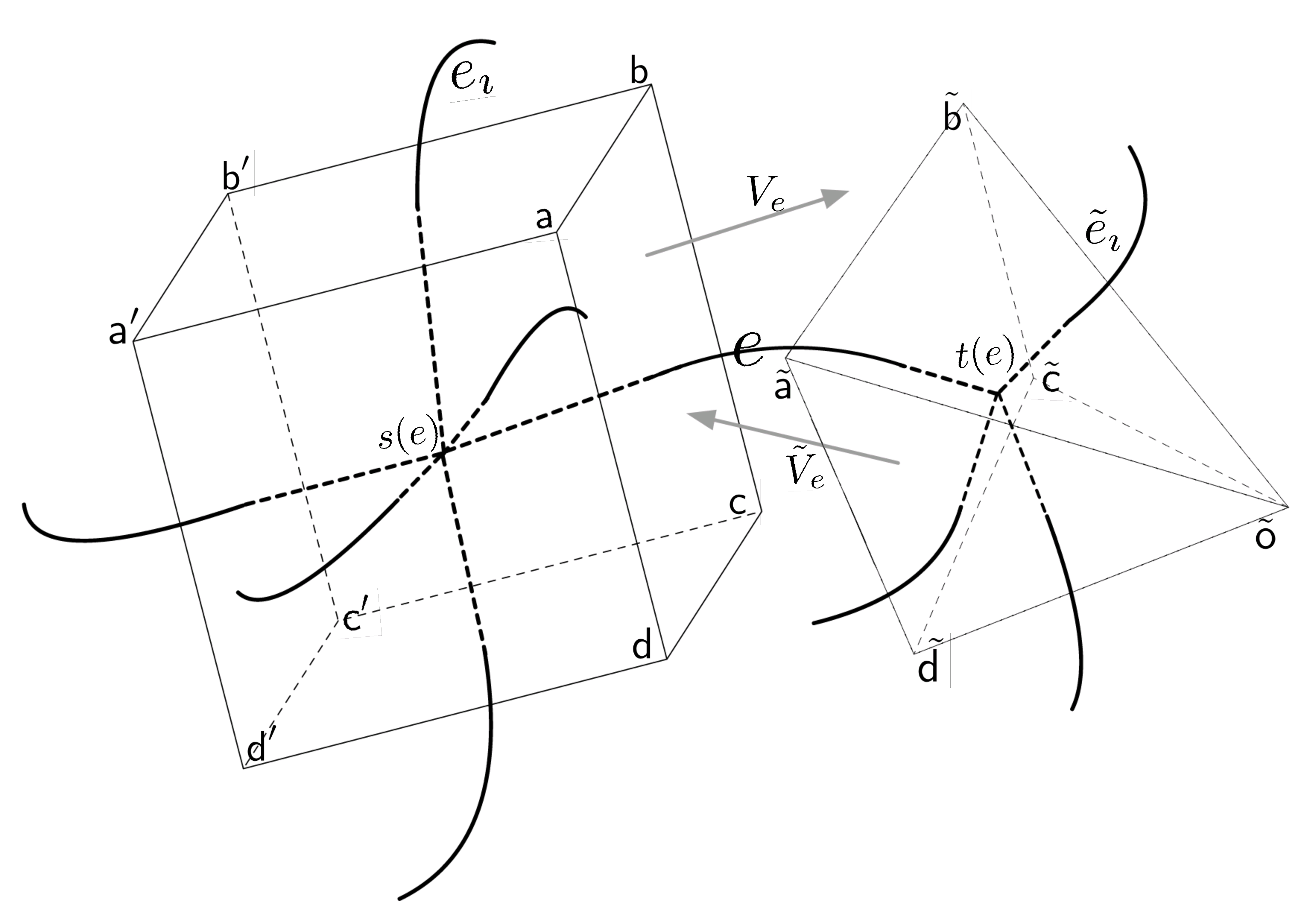
Figure 1: This figure shows the geometric interpretation of each factor in the expression $h_{e}^{\Gamma}=n_{e}(V_{e})e^{\zeta_{e}\tau_{3}}\tilde{n}_{e}(\tilde{V}_{e})^{-1}$. The source point $s(e)$ of edge $e$ is dual to a hexahedron $\textsf{a}\textsf{b}\textsf{c}\textsf{d}\textsf{a}^{\prime}\textsf{b}^{\prime}\textsf{c}^{\prime}\textsf{d}^{\prime}$ and the target point $t(e)$ of edge $e$ is dual to a quadrangular pyramid $\tilde{\textsf{a}}\tilde{\textsf{b}}\tilde{\textsf{c}}\tilde{\textsf{d}}\tilde{\textsf{o}}$, and edge $e$ is dual to the two faces abcd and $\tilde{\textsf{a}}\tilde{\textsf{b}}\tilde{\textsf{c}}\tilde{\textsf{d}}$, with abcd and $\tilde{\textsf{a}}\tilde{\textsf{b}}\tilde{\textsf{c}}\tilde{\textsf{d}}$ belonging to the hexahedron $\textsf{a}\textsf{b}\textsf{c}\textsf{d}\textsf{a}^{\prime}\textsf{b}^{\prime}\textsf{c}^{\prime}\textsf{d}^{\prime}$ and quadrangular pyramid $\tilde{\textsf{a}}\tilde{\textsf{b}}\tilde{\textsf{c}}\tilde{\textsf{d}}\tilde{\textsf{o}}$ respectively. The spin connection holonomy $h_{e}^{\Gamma}=n_{e}(V_{e})e^{\zeta_{e}\tau_{3}}\tilde{n}_{e}(\tilde{V}_{e})^{-1}$ tells us how to glue the hexahedron $\textsf{a}\textsf{b}\textsf{c}\textsf{d}\textsf{a}^{\prime}\textsf{b}^{\prime}\textsf{c}^{\prime}\textsf{d}^{\prime}$ and quadrangular pyramid $\tilde{\textsf{a}}\tilde{\textsf{b}}\tilde{\textsf{c}}\tilde{\textsf{d}}\tilde{\textsf{o}}$ by matching the two faces abcd and $\tilde{a}\tilde{b}\tilde{c}\tilde{d}$. Specifically, $n_{e}(V_{e})^{-1}$ rotates the hexahedron $\textsf{a}\textsf{b}\textsf{c}\textsf{d}\textsf{a}^{\prime}\textsf{b}^{\prime}\textsf{c}^{\prime}\textsf{d}^{\prime}$ to ensure that the outward and unit normal vector $V^{i}_{e}$ of the face abcd equals to the unit vector $\delta_{3}^{i}$, while $\tilde{n}_{e}(\tilde{V}_{e})^{-1}$ rotates the quadrangular pyramid $\tilde{\textsf{a}}\tilde{\textsf{b}}\tilde{\textsf{c}}\tilde{\textsf{d}}\tilde{\textsf{o}}$ to ensure that the outward and unit normal vector $\tilde{V}^{i}_{e}$ of the face $\tilde{\textsf{a}}\tilde{\textsf{b}}\tilde{\textsf{c}}\tilde{\textsf{d}}$ to the unit vector $-\delta_{3}^{i}$. Moreover, with $V_{e}^{i}=-\tilde{V}_{e}^{i}=\delta_{3}^{i}$, $e^{\zeta_{e}\tau_{3}}$ rotates the quadrangular pyramid $\tilde{\textsf{a}}\tilde{\textsf{b}}\tilde{\textsf{c}}\tilde{\textsf{d}}\tilde{\textsf{o}}$ to ensure that an edge of the face $\tilde{\textsf{a}}\tilde{\textsf{b}}\tilde{\textsf{c}}\tilde{\textsf{d}}$ is parallel to its corresponding edge in the face abcd. The two edges from the faces abcd and $\tilde{\textsf{a}}\tilde{\textsf{b}}\tilde{\textsf{c}}\tilde{\textsf{d}}$, which will be parallel to each other with the rotation of $\tilde{\textsf{a}}\tilde{\textsf{b}}\tilde{\textsf{c}}\tilde{\textsf{d}}\tilde{\textsf{o}}$ by $e^{\zeta_{e}\tau_{3}}$, can be determined by choosing a minimal loop containing $e$. For instance, one can chooses the minimal loop $\square_{\imath}$ containing $e$, $e_{\imath}$ and $\tilde{e}_{\imath}$, and then edges $\tilde{\textsf{a}}\tilde{\textsf{b}}$ and ab dual to $\square_{\imath}$ will be parallel to each other with the rotation of $\tilde{\textsf{a}}\tilde{\textsf{b}}\tilde{\textsf{c}}\tilde{\textsf{d}}\tilde{\textsf{o}}$ by $e^{\zeta_{e}\tau_{3}}$. Thus, $e^{\zeta_{e}\tau_{3}}$ is dependent on the choice of the minimal loop containing $e$. If the shape of the faces abcd and $\tilde{\textsf{a}}\tilde{\textsf{b}}\tilde{\textsf{c}}\tilde{\textsf{d}}$ are matched to each other, the twisted geometry on $e$ will be referred as to the shape-matching twisted geometry on $e$. Then, it is easy to see that $e^{\zeta_{e}\tau_{3}}$ is independent of the choice the minimal loop for the shape-matching twisted geometry on $e$.

Notice that $n_{e}(V_{e})$ is a function of $V_{e}=V_{e}^{i}$, which reads

$$n_{e}(V_{e})=\cos(\theta_{e}/2)\mathbb{I}-\mathbf{i}\sin(\theta_{e}/2)\sigma(V_{e}),$$ (33)

where $\cos\theta_{e}:=V_{e}^{3}=V_{e}^{i}\delta_{3}^{j}\delta_{ij}$, $\sigma(V_{e}):=\frac{1}{\sin\theta_{e}}\delta_{3}^{i}V_{e}^{j}\epsilon_{ijk}\sigma^{k}$ with $\sin\theta_{e}=|\delta_{3}^{i}V_{e}^{j}\epsilon_{ijk}|$ and $0\leq\theta_{e}<\pi$. One can further express $n_{e}(V_{e})$ as

$$n_{e}(V_{e})=\sqrt{\frac{1+V_{e}^{3}}{2}}\mathbb{I}-\mathbf{i}\sqrt{\frac{1}{2(1+V_{e}^{3})}}(V_{e}^{1}\sigma^{2}-V_{e}^{2}\sigma^{1}).$$ (34)

and $n_{e}(V_{e})^{-1}$ as

$$n_{e}(V_{e})^{-1}=\cos(\theta_{e}/2)\mathbb{I}+\mathbf{i}\sin(\theta_{e}/2)\sigma(V_{e})=\sqrt{\frac{1+V_{e}^{3}}{2}}\mathbb{I}+\mathbf{i}\sqrt{\frac{1}{2(1+V_{e}^{3})}}(V_{e}^{1}\sigma^{2}-V_{e}^{2}\sigma^{1}).$$ (35)

Similarly, $\tilde{n}_{e}(\tilde{V}_{e})$ is a function of $\tilde{V}_{e}^{\imath}$ given by

$$\tilde{n}_{e}(\tilde{V}_{e})=\cos(\tilde{\theta}_{e}/2)\mathbb{I}+\mathbf{i}\sin(\tilde{\theta}_{e}/2)\sigma(\tilde{V}_{e}),$$ (36)

where $\cos\tilde{\theta}_{e}:=-\tilde{V}_{e}^{3}=-\tilde{V}_{e}^{i}\delta_{3}^{j}\delta_{ij}$, $\sigma(\tilde{V}_{e}):=\frac{1}{\sin\tilde{\theta}_{e}}\delta_{3}^{i}\tilde{V}_{e}^{j}\epsilon_{ijk}\sigma^{k}$ with $\sin\tilde{\theta}_{e}=|\delta_{3}^{i}\tilde{V}_{e}^{j}\epsilon_{ijk}|$ and $0\leq\tilde{\theta}_{e}<\pi$. We also express $\tilde{n}_{e}(\tilde{V}_{e})$ and $\tilde{n}_{e}(\tilde{V}_{e})^{-1}$ as

$$\tilde{n}_{e}(\tilde{V}_{e})=\sqrt{\frac{1-\tilde{V}_{e}^{3}}{2}}\mathbb{I}+\mathbf{i}\sqrt{\frac{1}{2(1-\tilde{V}_{e}^{3})}}(\tilde{V}_{e}^{1}\sigma^{2}-\tilde{V}_{e}^{2}\sigma^{1}),$$ (37)

and

$$\tilde{n}_{e}(\tilde{V}_{e})^{-1}=\sqrt{\frac{1-\tilde{V}_{e}^{3}}{2}}\mathbb{I}-\mathbf{i}\sqrt{\frac{1}{2(1-\tilde{V}_{e}^{3})}}(\tilde{V}_{e}^{1}\sigma^{2}-\tilde{V}_{e}^{2}\sigma^{1}),$$ (38)

respectively.

Now, let us turn to express $e^{\zeta_{e}\tau_{3}}$ in terms of fluxes. Notice that $e^{\zeta_{e}\tau_{3}}$ relies on a minimal loop containing $e$, we can choose the minimal loop $\square_{\imath}$ containing $e$, $e_{\imath}$ and $\tilde{e}_{\imath}$ without loss of generality, see more details in Fig.1. Then, one can define

$$\check{V}_{e_{\imath}}^{i}:=-2\text{tr}(\tau^{i}n_{e}^{-1}\tau_{j}n_{e})\breve{V}_{e_{\imath}}^{j}=\frac{\bar{V}_{e_{\imath}}^{i}-{V}_{e_{\imath}}^{k}V_{e,k}\delta_{3}^{i}}{\sqrt{1-({V}_{e_{\imath}}^{k}V_{e,k})^{2}}}$$ (39)

at the source point of $e$, where $\breve{V}_{e_{\imath}}^{j}:=\frac{{V}_{e_{\imath}}^{j}-{V}_{e_{\imath}}^{k}V_{e,k}V_{e}^{j}}{\sqrt{1-({V}_{e_{\imath}}^{k}V_{e,k})^{2}}}$, $e_{\imath}$ is reoriented to be started at $s(e)$, and

$$\bar{V}_{e_{\imath}}^{i} := -2\text{tr}(\tau^{i}n_{e}^{-1}\tau_{j}n_{e}){V}_{e_{\imath}}^{j}$$

$$= \frac{\delta_{3}^{j}V_{e}^{k}{\epsilon_{jk}}^{i}}{\sin^{2}\theta_{e}}\delta_{3}^{i^{\prime}}V_{e}^{j^{\prime}}\epsilon_{i^{\prime}j^{\prime}k^{\prime}}{V}_{{e}_{\imath}}^{k^{\prime}}+2\delta_{3}^{[i}V_{e}^{j]}{V}_{{e}_{\imath},j}-4\delta_{3}^{[i}V_{e}^{k]}\delta_{kk^{\prime}}\delta_{3}^{[k^{\prime}}V_{e}^{j]}{V}_{{e}_{\imath},j}\frac{\cos\theta_{e}}{\sin^{2}\theta_{e}}$$

$$= \frac{\delta_{3}^{j}V_{e}^{k}{\epsilon_{jk}}^{i}}{1-(V_{e}^{3})^{2}}(V_{e}^{1}{V}_{{e}_{\imath}}^{2}-V_{e}^{2}{V}_{{e}_{\imath}}^{1})+\frac{1-2(V_{e}^{3})^{2}}{1-(V_{e}^{3})^{2}}\delta_{3}^{i}V_{e}^{j}{V}_{{e}_{\imath},j}$$

$$+\frac{V_{e}^{3}}{1-(V_{e}^{3})^{2}}\delta_{3}^{i}V_{e,k^{\prime}}V_{e}^{k^{\prime}}{V}^{3}_{{e}_{\imath}}+\frac{V_{e}^{3}}{1-(V_{e}^{3})^{2}}V_{e}^{i}V_{e}^{j}{V}_{{e}_{\imath},j}-\frac{1}{1-(V_{e}^{3})^{2}}V_{e}^{i}{V}^{3}_{{e}_{\imath}}.$$

Also, let us define

$$\check{V}_{\tilde{e}_{\imath}}^{i}:=-2\text{tr}(\tau^{i}\tilde{n}_{e}^{-1}\tau_{j}\tilde{n}_{e})\breve{V}_{\tilde{e}_{\imath}}^{j}=\frac{\bar{V}_{\tilde{e}_{\imath}}^{i}+{V}_{\tilde{e}_{\imath}}^{k}\tilde{V}_{e,k}\delta_{3}^{i}}{\sqrt{1-({V}_{\tilde{e}_{\imath}}^{k}\tilde{V}_{e,k})^{2}}}$$ (41)

at the target point of $e$, where $\breve{V}_{\tilde{e}_{\imath}}^{j}:=\frac{{V}_{\tilde{e}_{\imath}}^{j}-{V}_{\tilde{e}_{\imath}}^{k}\tilde{V}_{e,k}\tilde{V}_{e}^{j}}{\sqrt{1-({V}_{\tilde{e}_{\imath}}^{k}\tilde{V}_{e,k})^{2}}}$, $\tilde{e}_{\imath}$ is reoriented to be started at $t(e)$, and

$$\bar{V}_{\tilde{e}_{\imath}}^{i} := -2\text{tr}(\tau^{i}\tilde{n}_{e}^{-1}\tau_{j}\tilde{n}_{e}){V}_{\tilde{e}_{\imath}}^{j}$$

$$= \frac{\delta_{3}^{j}\tilde{V}_{e}^{k}{\epsilon_{jk}}^{i}}{\sin^{2}\tilde{\theta}_{e}}\delta_{3}^{i^{\prime}}\tilde{V}_{e}^{j^{\prime}}\epsilon_{i^{\prime}j^{\prime}k^{\prime}}{V}_{\tilde{e}_{\imath}}^{k^{\prime}}-2\delta_{3}^{[i}\tilde{V}_{e}^{j]}{V}_{\tilde{e}_{\imath},j}-4\delta_{3}^{[i}\tilde{V}_{e}^{k]}\delta_{kk^{\prime}}\delta_{3}^{[k^{\prime}}\tilde{V}_{e}^{j]}{V}_{\tilde{e}_{\imath},j}\frac{\cos\tilde{\theta}_{e}}{\sin^{2}\tilde{\theta}_{e}}$$

$$= \frac{\delta_{3}^{j}\tilde{V}_{e}^{k}{\epsilon_{jk}}^{i}}{1-(\tilde{V}_{e}^{3})^{2}}(\tilde{V}_{e}^{1}{V}_{\tilde{e}_{\imath}}^{2}-\tilde{V}_{e}^{2}{V}_{\tilde{e}_{\imath}}^{1})+\frac{2(\tilde{V}_{e}^{3})^{2}-1}{1-(\tilde{V}_{e}^{3})^{2}}\delta_{3}^{i}\tilde{V}_{e}^{j}{V}_{\tilde{e}_{\imath},j}$$

$$-\frac{\tilde{V}_{e}^{3}}{1-(\tilde{V}_{e}^{3})^{2}}\delta_{3}^{i}\tilde{V}_{e}^{k}\tilde{V}_{e,k}{V}_{\tilde{e}_{\imath},3}+\frac{\tilde{V}_{e}^{i}{V}_{\tilde{e}_{\imath}}^{3}}{1-(\tilde{V}_{e}^{3})^{2}}-\frac{\tilde{V}_{e}^{i}\tilde{V}_{e}^{3}}{1-(\tilde{V}_{e}^{3})^{2}}\tilde{V}_{e}^{j}{V}_{\tilde{e}_{\imath},j}.$$

Then, $e^{\zeta_{e}\tau_{3}}$ takes the formulation

$$e^{\zeta_{e}\tau_{3}}=\cos(\zeta_{e}/2)\mathbb{I}-\mathbf{i}\sin(\zeta_{e}/2)\sigma_{3}$$ (43)

with

$$\cos(\zeta_{e}/2)=\sqrt{\frac{1+\cos\zeta_{e}}{2}},\quad\sin(\zeta_{e}/2)=\text{sgn}(\zeta_{e})\sqrt{\frac{1-\cos\zeta_{e}}{2}},$$ (44)

where $\zeta_{e}\in(-\pi,\pi]$, $\cos\zeta_{e}$ and $\text{sgn}(\zeta_{e})$ are given by

$$\cos\zeta_{e}=\check{V}_{\tilde{e}_{\imath}}^{i}\check{V}_{e_{\imath}}^{j}\delta_{ij}=\frac{\bar{V}_{e_{\imath}}^{i}\bar{V}_{\tilde{e}_{\imath}}^{j}\delta_{ij}-{V}_{e_{\imath}}^{k}V_{e,k}\bar{V}_{\tilde{e}_{\imath}}^{3}+{V}_{\tilde{e}_{\imath}}^{k}\tilde{V}_{e,k}\bar{V}_{e_{\imath}}^{3}-{V}_{\tilde{e}_{\imath}}^{k}\tilde{V}_{e,k}{V}_{e_{\imath}}^{l}V_{e,l}}{\sqrt{1-({V}_{e_{\imath}}^{k}V_{e,k})^{2}}\sqrt{1-({V}_{\tilde{e}_{\imath}}^{k}\tilde{V}_{e,k})^{2}}}$$ (45)

and

$$\text{sgn}(\zeta_{e})=\text{sgn}(\epsilon_{ijk}\delta_{3}^{i}\check{V}_{\tilde{e}_{\imath}}^{j}\check{V}_{e_{\imath}}^{k})=\text{sgn}(\epsilon_{ijk}\delta_{3}^{i}\bar{V}_{\tilde{e}_{\imath}}^{j}\bar{V}_{e_{\imath}}^{k})$$ (46)

respectively.

Now, $h_{e}^{\Gamma}$ can be expressed as

$$h_{e}^{\Gamma}=n_{e}(V_{e})e^{\zeta_{e}\tau_{3}}\tilde{n}_{e}(\tilde{V}_{e})^{-1}$$

$$= \left(\sqrt{\frac{1+V_{e}^{3}}{2}}\mathbb{I}-\mathbf{i}\sqrt{\frac{1}{2(1+V_{e}^{3})}}(V_{e}^{1}\sigma^{2}-V_{e}^{2}\sigma^{1})\right)\left(\cos(\zeta_{e}/2)\mathbb{I}-\mathbf{i}\sin(\zeta_{e}/2)\sigma_{3}\right)$$

$$\cdot\left(\sqrt{\frac{1-\tilde{V}_{e}^{3}}{2}}\mathbb{I}-\mathbf{i}\sqrt{\frac{1}{2(1-\tilde{V}_{e}^{3})}}(\tilde{V}_{e}^{1}\sigma^{2}-\tilde{V}_{e}^{2}\sigma^{1})\right)$$

$$= w_{0}(\Gamma_{e})\mathbb{I}+w_{1}(\Gamma_{e})\mathbf{i}\sigma_{1}+w_{2}(\Gamma_{e})\mathbf{i}\sigma_{2}+w_{3}(\Gamma_{e})\mathbf{i}\sigma_{3},$$

where we defined

$$w_{0}(\Gamma_{e}) := -\sin(\zeta_{e}/2)\sqrt{\frac{1}{2(1+V_{e}^{3})}}\sqrt{\frac{1}{2(1-\tilde{V}_{e}^{3})}}(V_{e}^{2}\tilde{V}_{e}^{1}-V_{e}^{1}\tilde{V}_{e}^{2})$$

$$+\cos(\zeta_{e}/2)\Big{(}\sqrt{\frac{1-\tilde{V}_{e}^{3}}{2}}\sqrt{\frac{1+V_{e}^{3}}{2}}-\sqrt{\frac{1}{2(1+V_{e}^{3})}}\sqrt{\frac{1}{2(1-\tilde{V}_{e}^{3})}}(V_{e}^{1}\tilde{V}_{e}^{1}+V_{e}^{2}\tilde{V}_{e}^{2})\Big{)},$$

$$w_{1}(\Gamma_{e}) := \cos(\zeta_{e}/2)\Big{(}\sqrt{\frac{1-\tilde{V}_{e}^{3}}{2}}\sqrt{\frac{1}{2(1+V_{e}^{3})}}V_{e}^{2}+\sqrt{\frac{1+V_{e}^{3}}{2}}\sqrt{\frac{1}{2(1-\tilde{V}_{e}^{3})}}\tilde{V}_{e}^{2}\Big{)}$$

$$+\sin(\zeta_{e}/2)\Big{(}\sqrt{\frac{1+V_{e}^{3}}{2}}\sqrt{\frac{1}{2(1-\tilde{V}_{e}^{3})}}\tilde{V}_{e}^{1}-\sqrt{\frac{1-\tilde{V}_{e}^{3}}{2}}\sqrt{\frac{1}{2(1+V_{e}^{3})}}V_{e}^{1}\Big{)},$$

$$w_{2}(\Gamma_{e}) := -\cos(\zeta_{e}/2)\Big{(}\sqrt{\frac{1+V_{e}^{3}}{2}}\sqrt{\frac{1}{2(1-\tilde{V}_{e}^{3})}}\tilde{V}_{e}^{1}+\sqrt{\frac{1-\tilde{V}_{e}^{3}}{2}}\sqrt{\frac{1}{2(1+V_{e}^{3})}}V_{e}^{1}\Big{)}$$

$$+\sin(\zeta_{e}/2)\Big{(}\sqrt{\frac{1+V_{e}^{3}}{2}}\sqrt{\frac{1}{2(1-\tilde{V}_{e}^{3})}}\tilde{V}_{e}^{2}-\sqrt{\frac{1-\tilde{V}_{e}^{3}}{2}}\sqrt{\frac{1}{2(1+V_{e}^{3})}}V_{e}^{2}\Big{)}$$

and

$$w_{3}(\Gamma_{e}) := -\cos(\zeta_{e}/2)\sqrt{\frac{1}{2(1+V_{e}^{3})}}\sqrt{\frac{1}{2(1-\tilde{V}_{e}^{3})}}(-V_{e}^{2}\tilde{V}_{e}^{1}+V_{e}^{1}\tilde{V}_{e}^{2})$$

$$+\sin(\zeta_{e}/2)\Big{(}-\sqrt{\frac{1-\tilde{V}_{e}^{3}}{2}}\sqrt{\frac{1+V_{e}^{3}}{2}}+\sqrt{\frac{1}{2(1+V_{e}^{3})}}\sqrt{\frac{1}{2(1-\tilde{V}_{e}^{3})}}(-V_{e}^{1}\tilde{V}_{e}^{1}-V_{e}^{2}\tilde{V}_{e}^{2})\Big{)}.$$

It should be noted that the holonomy $h_{e}^{\Gamma}$ of the spin connection given by Eq.(3.1) involves a minimal loop $\square_{\imath}$ containing $e$, $e_{\imath}$ and $\tilde{e}_{\imath}$. Indeed, as shown in Fig.1, if the shapes of the two faces dual to $e$ are matched, we claim that the twisted geometry on $e$ satisfies the shape-matching condition, and then the holonomy $h_{e}^{\Gamma}$ is independent of the choice of the minimal loop $\square_{\imath}$. In general, the twisted geometry cannot ensure that the shape-matching condition holds for every edge, so the holonomy $h_{e}^{\Gamma}$ of the spin connection is expressed with its dependence on a minimal loop containing $e$. In the next subsection we will show that there is a natural choice of the minimal loop for $h_{e}^{\Gamma}$ when it appears in the expression of the discrete spatial scalar curvature.

3.2 Spatial scalar curvature in terms of twisted geometry

The holonomy of the spin connection in terms of flux variables helps us to regularize the densitized scalar curvature $\sqrt{q}R=-\sqrt{q}R_{ab}^{j}\epsilon_{jkl}e^{ak}e^{bl}$ of the spatial metric $q_{ab}$, where $R_{ab}^{j}:=2\partial_{[a}\Gamma_{b]}^{j}+\epsilon^{j}_{\ kl}\Gamma_{a}^{k}\Gamma^{l}_{b}$. Consider a cubic graph $\gamma_{\square}$ with the coordinate length of each elementary edge being given by $\mu$, the integral $\tilde{R}=\int_{\Sigma}dx\sqrt{q}R(x)$ can be given by

$$\tilde{R}=\int_{\Sigma}dx\sqrt{q}R(x)=-\int_{\Sigma}dxR_{ab}^{j}\epsilon_{jkl}\sqrt{q}e^{ak}e^{bl}=\lim_{\mu\to 0}\sum_{v\in\gamma_{\square}}R_{\square_{v}}$$ (52)

with $R_{\square_{v}}$ being given by

$$R_{\square_{v}}=\frac{(\beta a^{2})^{2}}{2}\sum_{\square_{e_{I},e_{J}}}\frac{p^{i}_{e_{I}}p^{j}_{e_{J}}}{V(v)}\epsilon_{ijk}\text{tr}(\tau^{k}h^{\Gamma}_{\square_{e_{I},e_{J}}})$$ (53)

where $\square_{e_{I},e_{J}}$ is a minimal loop containing edges $e_{I}$ and $e_{J}$, which begins at $v$ via $e_{I}$ and gets back to $v$ through $e_{J}$. The second “$=$” in Eq.(52) is from the continuum limit $\sqrt{q}R|_{v}=\lim_{\mu\to 0}\frac{R_{\square_{v}}}{\mu^{3}}$, which will be proven in next subsection. Notice that $\frac{p^{i}_{e_{I}}p^{j}_{e_{J}}}{V(v)}$ contains the inverse volume which complicates the expression. To avoid this problem, one can use Thiemann’s trick

$$\epsilon_{jkl}\sqrt{q}e^{ak}e^{bl}=\epsilon^{abc}e_{cj}=2\epsilon^{abc}\{A_{cj}(x),V(x)\}/(\kappa\beta)$$ (54)

to get another expression of $\tilde{R}$, where $V(x):=\int_{D}dy\sqrt{q}$ with $D\ni x$. We have

$$\tilde{R}=\int_{\Sigma}dx\sqrt{q}R(x)=-\frac{2}{\kappa\beta}\int_{\Sigma}dxR_{ab}^{j}\epsilon^{abc}\{A_{cj}(x),V(x)\}=\lim_{\mu\to 0}\sum_{v\in\gamma_{\square}}R_{\square_{v}}$$ (55)

with

$$R_{\square_{v}}=-\frac{4}{\kappa\beta}\sum_{e_{I},e_{J},e_{K}\in\gamma_{\square}}^{e_{I}\cap e_{J}\cap e_{K}=v}\epsilon^{IJK}\text{tr}(h_{e_{K}}\{h^{-1}_{e_{K}},V(v)\}h^{\Gamma}_{\square_{e_{I},e_{J}}}),$$ (56)

where $e_{I},e_{J},e_{K}$ have been re-oriented to be outgoing at $v$, $\epsilon^{IJK}=\text{sgn}[\det(e_{I}\wedge e_{J}\wedge e_{K})]$, $\square_{e_{I},e_{J}}$ is the minimal loop around a plaquette containing $e_{I}$ and $e_{J}$, which begins at $v$ via $e_{I}$ and gets back to $v$ through $e_{J}$.

3.3 Geometric interpretation of $h_{e}^{\Gamma}$ and $R_{\square_{v}}$ from the continuum limit

3.3.1 Spin connection and scalar curvature in terms of triad

Recall the expression of the spin connection

$$\Gamma_{ajk}=-(\partial_{a}e_{bj}-\Gamma_{ab}^{c}e_{cj})e^{b}_{k},$$ (57)

which can also be expressed in terms of of $e_{a}^{i}$ as

$$\Gamma_{a}^{i}=\frac{1}{2}\epsilon^{ijk}e_{k}^{b}(\partial_{b}e_{aj}-\partial_{a}e_{bj}+e^{c}_{j}e_{al}\partial_{b}e^{l}_{c}),$$ (58)

with $\Gamma_{a}^{i}\epsilon_{ijk}\equiv\Gamma_{ajk}$. Notice that the coordinate components of $\Gamma_{ab}^{c}$ transforms as a connection under the coordinate transformation. Let us introduce a regular coordinate system $\{x_{I}|I\in\{1,2,3\}\}|_{p}$ in a small open neighborhood of point $p$, which satisfies

$$\Gamma_{x_{I}x_{J}}^{c}|_{p}\equiv(\frac{\partial}{\partial x_{I}})^{a}(\frac{\partial}{\partial x_{J}})^{b}\Gamma_{ab}^{c}|_{p}=0,\quad\forall I\neq J.$$ (59)

This regular coordinate system $\{x_{I}|J\in\{1,2,3\}\}|_{p}$ can also be determined in a different way. Notice $\Gamma_{ajk}$ transforms as a connection under the gauge transformation. Then, the regular coordinate system $\{x_{I}|J\in\{1,2,3\}\}|_{p}$ can be determined by requiring

$$\partial_{x_{2}}e_{x_{1}j}|_{p}=\partial_{x_{2}}e_{x_{3}j}|_{p}=\partial_{x_{3}}e_{x_{1}j}|_{p}=\partial_{x_{3}}e_{x_{2}j}|_{p}=\partial_{x_{1}}e_{x_{2}j}|_{p}=\partial_{x_{1}}e_{x_{3}j}|_{p}=0$$ (60)

for the gauge choice

$$\Gamma_{ajk}|_{p}=0.$$ (61)

It is easy to verify that the regular coordinate systems $\{x_{I}|I\in\{1,2,3\}\}|_{p}$ determined by condition (59) or (60) are equivalent to each other, by using the definition of spin connection (57). Moreover, one should notice that once the regular coordinate system is determined by using the conditions (61) and (60), the gauge fixing condition (61) can be released, since the gauge transformation of $\Gamma_{ajk}$ is independent with the coordinate transformation.

Now, we can simplify the expression of $\Gamma_{a}^{i}|_{p}$ in this regular coordinate system $\{x_{I}|I\in\{1,2,3\}\}$ as follows. Denoted by $\Gamma_{x_{I}jk}\equiv(\frac{\partial}{\partial x_{I}})^{a}\Gamma_{ajk}|$. Notice that $\Gamma_{ajk}$ transforms as a connection under the gauge transformation, and thus one can make a gauge transformation which leads

$$\Gamma_{x_{1}jk}|_{p}\mapsto\Gamma_{x_{1}jk}|_{p},\quad\Gamma_{x_{2}jk}|_{p}\mapsto 0,\quad\Gamma_{x_{3}jk}|_{p}\mapsto 0.$$ (62)

Then, it is straightforwardly to get

$$\partial_{x_{2}}e_{x_{1}j}|_{p}=\partial_{x_{2}}e_{x_{3}j}|_{p}=\partial_{x_{3}}e_{x_{1}j}|_{p}=\partial_{x_{3}}e_{x_{2}j}|_{p}=0$$ (63)

by using

$$\Gamma_{x_{I}jk}|_{p}\equiv(\frac{\partial}{\partial x_{I}})^{a}\Gamma_{ajk}|_{p}=-(\partial_{x_{I}}e_{bj}-\Gamma_{x_{I}b}^{c}e_{cj})e^{b}_{k}|_{p},$$ (64)

and the gauge condition (59) and (62). With the two conditions (59) and (62), the expression of $\Gamma_{x_{1}}^{i}|_{p}$ can be simplified as

$$\Gamma_{x_{1}}^{i}|_{p} \equiv (\frac{\partial}{\partial x_{1}})^{a}\Gamma_{a}^{i}|_{p}=\frac{1}{2}\epsilon^{ijk}e_{k}^{b}(\partial_{b}e_{x_{1}j}-\partial_{x_{1}}e_{bj}+e^{c}_{j}e_{x_{1}l}\partial_{b}e^{l}_{c})|_{p}$$

$$= \frac{1}{2}\epsilon^{ijk}(-e_{k}^{x_{2}}\partial_{x_{1}}e_{x_{2}j}-e_{k}^{x_{3}}\partial_{x_{1}}e_{x_{3}j})|_{p}$$

$$+\frac{1}{2}\epsilon^{ijk}e_{k}^{x_{1}}(e^{x_{2}}_{j}e_{x_{1}l}\partial_{x_{1}}e^{l}_{x_{2}})|_{p}+\frac{1}{2}\epsilon^{ijk}e_{k}^{x_{1}}(e^{x_{3}}_{j}e_{x_{1}l}\partial_{x_{1}}e^{l}_{x_{3}})|_{p}$$

by using Eq.(63). Though the expression (3.3.1) of $\Gamma_{x_{1}}^{i}|_{p}$ is given by considering the gauge transformation (62), it is valid for arbitrary gauge choice since the gauge transformation (62) does not change $\Gamma_{x_{1}}^{i}|_{p}$. Similarly, one can give the expression of $\Gamma_{x_{2}}^{i}|_{p}\equiv{\frac{\partial}{\partial x_{2}}}^{a}\Gamma_{a}^{i}|_{p}$ and $\Gamma_{x_{3}}^{i}|_{p}\equiv{\frac{\partial}{\partial x_{3}}}^{a}\Gamma_{a}^{i}|_{p}$ in the regular coordinate system $\{x_{I}|I\in\{1,2,3\}\}$, which read,

$$\Gamma_{x_{2}}^{i}|_{p} \equiv (\frac{\partial}{\partial x_{2}})^{a}\Gamma_{a}^{i}|_{p}=\frac{1}{2}\epsilon^{ijk}e_{k}^{b}(\partial_{b}e_{x_{2}j}-\partial_{x_{2}}e_{bj}+e^{c}_{j}e_{x_{2}l}\partial_{b}e^{l}_{c})|_{p}$$

$$= \frac{1}{2}\epsilon^{ijk}(-e_{k}^{x_{1}}\partial_{x_{2}}e_{x_{1}j}-e_{k}^{x_{3}}\partial_{x_{2}}e_{x_{3}j})|_{p}$$

$$+\frac{1}{2}\epsilon^{ijk}e_{k}^{x_{2}}(e^{x_{1}}_{j}e_{x_{2}l}\partial_{x_{2}}e^{l}_{x_{1}})|_{p}+\frac{1}{2}\epsilon^{ijk}e_{k}^{x_{2}}(e^{x_{3}}_{j}e_{x_{2}l}\partial_{x_{2}}e^{l}_{x_{3}})|_{p}$$

and

$$\Gamma_{x_{3}}^{i}|_{p} \equiv (\frac{\partial}{\partial x_{3}})^{a}\Gamma_{a}^{i}|_{p}=\frac{1}{2}\epsilon^{ijk}e_{k}^{b}(\partial_{b}e_{x_{3}j}-\partial_{x_{3}}e_{bj}+e^{c}_{j}e_{x_{3}l}\partial_{b}e^{l}_{c})|_{p}$$

$$= \frac{1}{2}\epsilon^{ijk}(-e_{k}^{x_{1}}\partial_{x_{3}}e_{x_{1}j}-e_{k}^{x_{2}}\partial_{x_{3}}e_{x_{2}j})|_{p}$$

$$+\frac{1}{2}\epsilon^{ijk}e_{k}^{x_{3}}(e^{x_{2}}_{j}e_{x_{3}l}\partial_{x_{3}}e^{l}_{x_{2}})|_{p}+\frac{1}{2}\epsilon^{ijk}e_{k}^{x_{3}}(e^{x_{1}}_{j}e_{x_{3}l}\partial_{x_{3}}e^{l}_{x_{1}})|_{p}.$$

Let us now consider the scalar curvature $R$ determined by the spatial metric $q_{ab}$. Using the equations (3.3.1),(3.3.1) and (3.3.1), one can try to express $R_{ab}^{j}|_{p}$ based on the triads and their derivatives in the regular coordinate system $\{x_{I}|I\in\{1,2,3\}\}|_{p}$. Note, however, that the derivative $\partial_{x_{K}}\Gamma_{x_{L}}^{j}|_{p}$ of the spin connection, which appears in the expression of $R_{x_{K}x_{L}}^{j}$, contains the information of $\Gamma_{x_{I}}^{j}$ beyond the point $p$, which leads to Eqs. (3.3.1),(3.3.1) and (3.3.1) for $\Gamma_{x_{I}}^{j}$ are not valid for the expression of $R_{x_{K}x_{L}}^{j}$.

To analyze the expression of the derivative $\partial_{x_{K}}\Gamma_{x_{L}}^{j}|_{p}$, consider the point $p^{\epsilon}_{K}$ whose coordinate satisfies $x_{I}(p^{\epsilon}_{K})=x_{I}(p)$ for $I\neq K$ and $x_{K}(p^{\epsilon}_{K})-x_{K}(p)=\epsilon$, where $\epsilon$ is small. Then, we have

$$\partial_{x_{K}}\Gamma_{x_{L}}^{j}|_{p}=\lim_{\epsilon\to 0}\frac{\Gamma_{x_{L}}^{j}|_{p^{\epsilon}_{K}}-\Gamma_{x_{L}}^{j}|_{p}}{\epsilon}.$$ (68)

It should be noted that the expression of $\Gamma_{x_{L}}^{j}|_{p^{\epsilon}_{K}}$ is not directly given by Eqs. (3.3.1), (3.3.1) and (3.3.1) directly, since the regular coordinate system $\{x_{I}|I\in\{1,2,3\}\}|_{p}$ for $p$ may not be a regular coordinate system for $p^{\epsilon}_{K}$. Nevertheless, one can always find a new coordinate system $\{\tilde{x}_{I}\}$ which satisfies that, (i) $\tilde{x}_{I}(p^{\epsilon}_{K})=x_{I}(p^{\epsilon}_{K})$, $\tilde{x}_{I}(p)=x_{I}(p),\forall I$, and (ii) $\Gamma^{\tilde{x}_{I}}_{\tilde{x}_{J}\tilde{x}_{L}}|_{p}=\Gamma^{\tilde{x}_{I}}_{\tilde{x}_{J}\tilde{x}_{L}}|_{p^{\epsilon}_{K}}=0$, $\forall J\neq L$, where $\Gamma^{\tilde{x}_{I}}_{\tilde{x}_{J}\tilde{x}_{L}}\equiv\Gamma^{a}_{bc}(d\tilde{x}_{I})_{a}(\frac{\partial}{\partial\tilde{x}_{J}})^{b}(\frac{\partial}{\partial\tilde{x}_{L}})^{c}$ and it is related to $\Gamma^{{x}_{P}}_{{x}_{M}{x}_{N}}$ by

$$\Gamma^{\tilde{x}_{I}}_{\tilde{x}_{J}\tilde{x}_{L}}=\sum_{M,N,P}\Gamma^{{x}_{P}}_{{x}_{M}{x}_{N}}\frac{\partial x_{M}}{\partial\tilde{x}_{J}}\frac{\partial x_{N}}{\partial\tilde{x}_{L}}\frac{\partial\tilde{x}_{I}}{\partial x_{P}}+\sum_{P}\frac{\partial^{2}x_{P}}{\partial\tilde{x}_{J}\partial\tilde{x}_{L}}\frac{\partial\tilde{x}_{I}}{\partial x_{P}}.$$ (69)

It is easy to see that the coordinate system $\{\tilde{x}_{I}\}$ satisfying above two conditions always exists, since the above two conditions for $\{\tilde{x}_{I}\}$ only involves specific two separate points.

Recalling the definition (59) of the regular coordinate system, it is easy to see that $\{\tilde{x}_{J}|J\in\{1,2,3\}\}|_{p,p^{\epsilon}_{K}}$ is a regular coordinate system for both $p$ and $p^{\epsilon}_{K}$. By taking $K=1,2,3$ step by step and establishing new coordinate system following the above procedures , we finally get a regular coordinate system $\{\tilde{\tilde{\tilde{x}}}_{J}|J\in\{1,2,3\}\}|_{p,p^{\epsilon}_{1},p^{\epsilon}_{2},p^{\epsilon}_{3}}$ for all of the points $p,p^{\epsilon}_{1},p^{\epsilon}_{2}$ and $p^{\epsilon}_{3}$. To simplify our notations, we will still denote by $\{x_{J}|J\in\{1,2,3\}\}|_{p,p^{\epsilon}_{1},p^{\epsilon}_{2},p^{\epsilon}_{3}}$ the regular coordinate system for $p,p^{\epsilon}_{1},p^{\epsilon}_{2}$ and $p^{\epsilon}_{3}$. Then, the expression of $\Gamma_{x_{L}}^{j}|_{p^{\epsilon}_{K}},\forall K$ can be given by Eqs. (3.3.1),(3.3.1) and (3.3.1) directly. Now, the scalar curvature $R$ at point $p$ can be expressed as

$$R|_{p}=-\sum_{K,L}R_{x_{K}x_{L}}^{j}\epsilon_{jmn}e^{x_{K}m}e^{x_{L}n}|_{p}$$ (70)

with

$$R_{x_{K}x_{L}}^{j}|_{p} = \partial_{x_{K}}\Gamma_{x_{L}}^{j}|_{p}-\partial_{x_{L}}\Gamma_{x_{K}}^{j}|_{p}+\epsilon^{j}_{\ mn}\Gamma_{x_{K}}^{m}\Gamma^{n}_{x_{L}}|_{p}$$ (71)

$$= \lim_{\epsilon\to 0}\frac{\Gamma_{x_{L}}^{j}|_{p^{\epsilon}_{K}}-\Gamma_{x_{L}}^{j}|_{p}}{\epsilon}-\lim_{\epsilon\to 0}\frac{\Gamma_{x_{K}}^{j}|_{p^{\epsilon}_{L}}-\Gamma_{x_{K}}^{j}|_{p}}{\epsilon}+\epsilon^{j}_{\ mn}\Gamma_{x_{K}}^{m}\Gamma^{n}_{x_{L}}|_{p}$$ (72)

where we used Eq.(68), $\Gamma_{x_{K}}^{j}|_{p}$, $\Gamma_{x_{L}}^{j}|_{p}$ and $\Gamma_{x_{K}}^{j}|_{p^{\epsilon}_{L}}$, $\Gamma_{x_{L}}^{j}|_{p^{\epsilon}_{K}}$ are given by Eqs. (3.3.1), (3.3.1) and (3.3.1). Notice that the expression (71) of $R_{x_{K}x_{L}}^{j}|_{p}$ relies on the regular coordinate system for both $p$ and the points $p^{\epsilon}_{K}$ near $p$. As we will seen in next subsection, such regular coordinate system appears in the shape-matching twisted geometry on cubic graph naturally, and it is crucial for the recovering of the expression (70) by the continuum limit of the discrete scalar curvature in the twisted geometry.

3.3.2 Continuum limit of $h_{e}^{\Gamma}$ and $R_{\square_{v}}$

Let us consider the continuum limit of the holonomy $h_{e}^{\Gamma}$ of spin connection on the edges in a cubic graph $\gamma_{\square}$, and focus on the configurations of twisted geometry which ensure that the shapes of the two faces dual to each edge are matched to each other. We first adapt the cubic graph $\gamma_{\square}$ to a coordinate system $\{\hat{x}_{I}|I\in\{1,2,3\}\}$, with the coordinate length of each elementary edge ${e}_{I}(v,\pm)$ of $\gamma_{\square}$ being set to $\mu$ and the coordinate basis field satisfying $(\frac{\partial}{\partial\hat{x}_{I}})^{a}=\dot{e}_{I}^{a}(v,\pm)$ on each ${e}_{I}(v,\pm)$, where the notation ${e}_{I}(v,\pm)$ ensures that $v$ is the source point of $e_{I}(v,+)$ and the target point of $e_{I}(v,-)$. For instance, one has $e_{1}=e_{1}(v_{1},+)=e_{1}(v_{2},-)$, $e_{2}=e_{2}(v_{1},-)=e_{2}(v_{3},+)$ and $e_{3}=e_{3}(v_{1},-)$ in figure 2.

Without loss of generality, our discussion will first focus on the single edge $e_{1}$ in figure 2. Then, we can introduce the following notations

$$w_{v_{1},\hat{x}_{1}}^{i}\equiv\overrightarrow{\textsf{a}^{\prime}\textsf{a}},\quad w_{v_{1},\hat{x}_{2}}^{i}\equiv\overrightarrow{\textsf{a}\textsf{d}},\quad w_{v_{1},\hat{x}_{3}}^{i}\equiv\overrightarrow{\textsf{a}\textsf{b}}$$ (73)

and

$$w_{v_{2},\hat{x}_{1}}^{i}\equiv\overrightarrow{\tilde{\textsf{a}}\tilde{\textsf{a}}^{\prime}},\quad w_{v_{2},\hat{x}_{2}}^{i}\equiv\overrightarrow{\tilde{\textsf{a}}\tilde{\textsf{d}}},\quad w_{v_{2},\hat{x}_{3}}^{i}\equiv\overrightarrow{\tilde{\textsf{a}}\tilde{\textsf{b}}}$$ (74)

for the vectors in figure 2. Correspondingly, one can define

$$w^{v_{1},\hat{x}_{1}}_{i}:=\frac{p_{e_{1},i}}{\text{V}(v_{1})},\quad w^{v_{1},\hat{x}_{2}}_{i}:=-\frac{\tilde{p}_{e_{2},i}}{\text{V}(v_{1})},\quad w^{v_{1},\hat{x}_{3}}_{i}:=-\frac{\tilde{p}_{e_{3},i}}{\text{V}(v_{1})}$$ (75)

where $\square_{v_{1}}$ is the hexahedron dual to $v_{1}$, and $\text{V}(v)$ is the volume of $\square_{v}$ defined by

$$\text{V}(v):=\sqrt{|\frac{1}{8}(\beta a^{2})^{3}\sum_{e\cap e^{\prime}\cap e^{\prime\prime}=v}\epsilon_{ijk}\epsilon_{e,e^{\prime},e^{\prime\prime}}p^{i}(v,e)p^{j}(v,e^{\prime})p^{k}(v,e^{\prime\prime})|}$$ (76)

with $\epsilon_{e,e^{\prime},e^{\prime\prime}}=\text{sgn}[\det(e\wedge e^{\prime}\wedge e^{\prime\prime})]$, $p^{i}(v,e)=p_{e}^{i}$ if $s(e)=v$ and $p^{i}(v,e)=-\tilde{p}_{e}^{i}$ if $t(e)=v$.

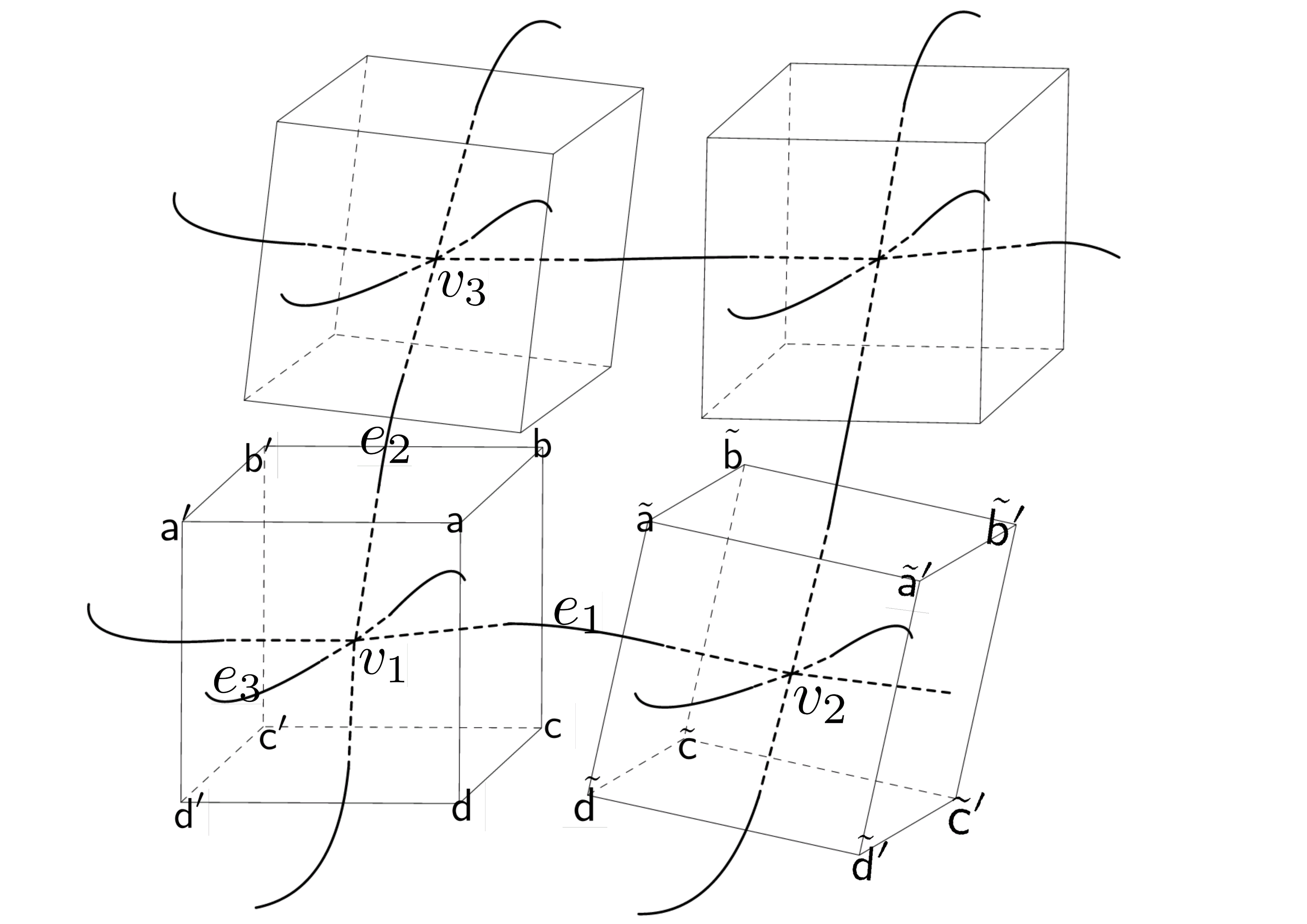
Figure 2: A part of the cubic graph and the dual Polyhedras at each vertices. The edges in the cubic graph have the notations $e_{1}=e_{1}(v_{1},+)=e_{1}(v_{2},-)$, $e_{2}=e_{2}(v_{1},-)=e_{2}(v_{3},+)$ and $e_{3}=e_{3}(v_{1},-)$.

Based on these notations and recall the geometric interpretation of each factor of $h_{e}^{\Gamma}=n_{e}(V_{e})e^{\zeta_{e}\tau_{3}}\tilde{n}_{e}(\tilde{V}_{e})^{-1}$ shown in Fig.1, one can check that the generator of $h_{e_{1}}^{\Gamma}=\exp(\Gamma_{e_{1}}^{i}\tau_{i})$ is given by

$$\Gamma_{e_{1}}^{i} = \frac{1}{2}\epsilon^{ijk}(-w_{k}^{v_{1},\hat{x}_{2}}{(w_{v_{2},\hat{x}_{2}j}-w_{v_{1},\hat{x}_{2}j})}-w_{k}^{v_{1},\hat{x}_{3}}{(w_{v_{2},\hat{x}_{3}j}-w_{v_{1},\hat{x}_{3}j})})(1+\mathcal{O}(\mu))$$

$$+\frac{1}{2}\epsilon^{ijk}w_{k}^{v_{1},\hat{x}_{1}}(w^{v_{1},\hat{x}_{2}}_{j}w_{v_{1},\hat{x}_{1}l}{(w^{l}_{v_{2},\hat{x}_{2}}-w^{l}_{v_{1},\hat{x}_{2}})})(1+\mathcal{O}^{\prime}(\mu))$$

$$+\frac{1}{2}\epsilon^{ijk}w_{k}^{v_{1},\hat{x}_{1}}(w^{v_{1},\hat{x}_{3}}_{j}w_{v_{1},\hat{x}_{1}l}{(w^{l}_{v_{2},\hat{x}_{3}}-w^{l}_{v_{1},\hat{x}_{3}})})(1+\mathcal{O}^{\prime\prime}(\mu))$$

for small $|\Gamma_{e_{1}}^{i}|\propto\mu$ with $\mu$ the lattice length scale. We leave the detailed check in Appendix A. Further, one can check that the spin connection along $e_{1}$ can be given by

$$\Gamma_{\hat{x}_{1}}^{i}|_{v_{1}} = \lim_{\mu\to 0}\frac{\Gamma_{e_{1}}^{i}}{\mu}$$

$$= \frac{1}{2}\epsilon^{ijk}(-e_{k}^{\hat{x}_{2}}\partial_{\hat{x}_{1}}e_{\hat{x}_{2}j}-e_{k}^{\hat{x}_{3}}\partial_{\hat{x}_{1}}e_{\hat{x}_{3}j})|_{v_{1}}$$

$$+\frac{1}{2}\epsilon^{ijk}e_{k}^{\hat{x}_{1}}(e^{\hat{x}_{2}}_{j}e_{\hat{x}_{1}l}\partial_{\hat{x}_{1}}e^{l}_{\hat{x}_{2}})|_{v_{1}}+\frac{1}{2}\epsilon^{ijk}e_{k}^{\hat{x}_{1}}(e^{\hat{x}_{3}}_{j}e_{\hat{x}_{1}l}\partial_{\hat{x}_{1}}e^{l}_{\hat{x}_{3}})|_{v_{1}}$$

by introducing the continuum limit

$$e^{\hat{x}_{I}}_{j}|_{v_{1}}=\lim_{\mu\to 0}(\mu w^{v_{1},\hat{x}_{I}}_{j}),\quad e_{\hat{x}_{I}}^{j}|_{v_{1}}=\lim_{\mu\to 0}\frac{w_{v_{1},\hat{x}_{I}}^{j}}{\mu}$$ (79)

and

$$\partial_{\hat{x}_{1}}e_{\hat{x}_{2}}^{i}|_{v_{1}}=\lim_{\mu\to 0}\frac{(w_{v_{2},\hat{x}_{2}}^{i}-w_{v_{1},\hat{x}_{2}}^{i})}{\mu^{2}},\quad\partial_{\hat{x}_{1}}e_{\hat{x}_{3}}^{i}|_{v_{1}}=\lim_{\mu\to 0}\frac{(w_{v_{2},\hat{x}_{3}}^{i}-w_{v_{1},\hat{x}_{3}}^{i})}{\mu^{2}}.$$ (80)

Finally, by comparing Eqs.(3.3.1) and (3.3.2), one can conclude that the continuum limit of the generator $\Gamma_{e_{1}}^{i}$ of $h_{e}^{\Gamma}$ reproduces the spin connection defined by triad exactly for the cubic graph.

However, it should be noted that Eq.(3.3.1) gives the expression of $\Gamma_{x_{1}}^{i}$ at $p$ based on the regular coordinate system $\{x_{I}\}$. Thus, one must require that $\{\hat{x}_{I}\}$ is also a regular coordinate system in the continuum limit to ensure the consistency of eqs.(3.3.1) and (3.3.2). In fact, for the shape-matching twisted geometry which ensures that the shapes of the two faces dual to each edge are matched to each other, one can immediately get that $\Gamma_{e_{1}}^{i}=0$ leads to $\Gamma_{\hat{x}_{1}}^{i}|_{v_{1}}=0$ and $\partial_{\hat{x}_{1}}e_{\hat{x}_{2}}^{i}=\partial_{\hat{x}_{1}}e_{\hat{x}_{3}}^{i}$ in the limit $\mu\to 0$, and this result can be generalized to $\Gamma_{e_{2}}^{i}=0$ and $\Gamma_{e_{3}}^{i}=0$ directly. Thus, the coordinate system $\{\hat{x}_{I}\}$ considered here is actually a regular coordinate system in the continuum limit for the shape-matched twisted geometry. Finally, one can conclude that the continuum limit of $h_{e}^{\Gamma}$ reproduces the spin connection defined by triad exactly for the cubic graph, at least for the shape-matching twisted geometry.

It is now ready to consider the continuum limit of $R_{\square_{v_{1}}}$ based on the continuum limit of $h_{e}^{\Gamma}$. Recall that the expression (53) of $R_{\square_{v_{1}}}$ is given by

$$R_{\square_{v_{1}}}=\frac{(\beta a^{2})^{2}}{2}\sum_{\square_{e_{I},e_{J}}}\frac{p^{i}_{e_{I}}p^{j}_{e_{J}}}{V(v_{1})}\epsilon_{ijk}\text{tr}(\tau^{k}h^{\Gamma}_{\square_{e_{I},e_{J}}})$$ (81)

on the cubic graph, where $\square_{e_{I},e_{J}}=e_{I}\circ e^{\prime}_{J}\circ e^{\prime}_{I}\circ e_{J}$, $e_{I}=e_{I}(v_{1},+)=e_{I}(v_{2},-),e^{\prime}_{J}=(e_{J}(v_{2},-))^{-1},e^{\prime}_{I}=(e_{I}(v_{3},+))^{-1},e_{J}=e_{J}(v_{1},-)=e_{J}(v_{3},+)$ as shown in Fig. 3, and $h^{\Gamma}_{\square_{e_{I},e_{J}}}=h^{\Gamma}_{e_{I}}h^{\Gamma}_{e^{\prime}_{J}}h^{\Gamma}_{e^{\prime}_{I}}h^{\Gamma}_{e_{J}}$. By using $h^{\Gamma}_{e_{I}}=\exp(\mu\Gamma_{e_{I}}^{i}\tau_{i})$, one can get

$$-2\text{tr}(\tau^{k}h^{\Gamma}_{\square_{e_{I},e_{J}}})=\mu^{2}(\frac{\Gamma^{k}_{e^{\prime}_{I}}+\Gamma^{k}_{e_{I}}}{\mu}+\frac{\Gamma^{k}_{e^{\prime}_{J}}+\Gamma^{k}_{e_{J}}}{\mu}-\epsilon^{k}_{\ mn}\Gamma^{m}_{e_{I}}\Gamma^{n}_{e_{J}})+\mathcal{O}({\mu^{3}}).$$ (82)

Thus, we have

$$\lim_{\mu\to 0}\frac{-2\text{tr}(\tau^{k}h^{\Gamma}_{\square_{e_{I},e_{J}}})}{\mu^{2}}$$

$$= \lim_{\mu\to 0}\frac{\Gamma^{k}_{a}\dot{e}^{\prime a}_{J}|_{v_{2}}+\Gamma^{k}_{b}\dot{e}^{b}_{J}|_{v_{1}}}{\mu}+\lim_{\mu\to 0}\frac{\Gamma^{k}_{a}\dot{e}^{\prime a}_{I}|_{v_{3}}+\Gamma^{k}_{b}\dot{e}^{b}_{I}|_{v}}{\mu}-\epsilon^{k}_{\ mn}\Gamma^{m}_{a}\dot{e}^{a}_{I}\Gamma^{n}_{b}\dot{e}^{b}_{J}|_{v_{1}},$$

where $v_{2}$ is the target point of $e_{I}$ and $v_{3}$ is the source point of $e_{J}$ as shown in Fig.3.

Figure 3: The minimal loop $\square_{e_{I},e_{J}}=e_{I}\circ e^{\prime}_{J}\circ e^{\prime}_{I}\circ e_{J}$ containing edges $e_{I}$ and $e_{J}$, which begins at $v_{1}$ via $e_{I}$ and gets back to $v_{1}$ through $e_{J}$.

Furthermore, by using Eq.(3.3.2), one get

$$\lim_{\mu\to 0}\frac{-2\text{tr}(\tau^{k}h^{\Gamma}_{\square_{e_{I},e_{J}}})}{\mu^{2}} = \lim_{\mu\to 0}\frac{\Gamma^{k}_{\hat{x}_{J}}|_{v_{2}}-\Gamma^{k}_{\hat{x}_{J}}|_{v_{1}}}{\mu}-\lim_{\mu\to 0}\frac{\Gamma^{k}_{\hat{x}_{I}}|_{v_{3}}-\Gamma^{k}_{\hat{x}_{I}}|_{v_{1}}}{\mu}+\epsilon^{k}_{\ mn}\Gamma^{m}_{\hat{x}_{I}}\Gamma^{n}_{\hat{x}_{J}}|_{v_{1}}$$

$$= \partial_{\hat{x}_{I}}\Gamma^{k}_{\hat{x}_{J}}|_{v_{1}}-\partial_{\hat{x}_{J}}\Gamma^{k}_{\hat{x}_{I}}|_{v_{1}}+\epsilon^{k}_{\ mn}\Gamma^{m}_{\hat{x}_{I}}\Gamma^{n}_{\hat{x}_{J}}|_{v_{1}}$$

$$= R_{\hat{x}_{I}\hat{x}_{J}}^{k}|_{v_{1}},$$

where we use Eq.(71) in the third “$=$” and the fact $R_{\hat{x}_{I}\hat{x}_{J}}^{k}|_{v_{1}}:=R_{ab}^{k}\dot{e}_{I}^{a}\dot{e}_{J}^{b}|_{v_{1}}$. Moreover, the continuum limit of the remaining factor $\frac{p^{i}_{e_{I}}p^{j}_{e_{J}}}{V(v_{1})}\epsilon_{ijk}$ in $R_{\square_{v_{1}}}$ is given by

$$\lim_{\mu\to 0}\frac{(\beta a^{2})^{2}}{\mu}\frac{p^{i}_{e_{I}}p^{j}_{e_{J}}}{V(v_{1})}\epsilon_{ijk} = |\det{(e)}|e^{\hat{x}_{I},i}e^{\hat{x}_{J},j}\epsilon_{ijk}|_{v_{1}},$$ (85)

where we used that $\lim_{\mu\to 0}\frac{V_{v_{1}}}{\mu^{3}}=|\det(e)|_{v_{1}}$ and $\lim_{\mu\to 0}\frac{\beta a^{2}p^{i}_{e_{I}}}{\mu^{2}}=|\det{(e)}|\cdot e^{\hat{x}_{I},i}|_{v_{1}}$ with $e^{\hat{x}_{I},i}|_{v_{1}}:=e^{ai}(d\hat{x}_{I})_{a}|_{v_{1}}$. Finally, we have the limit

$$\lim_{\mu\to 0}\frac{R_{\square_{v_{1}}}}{\mu^{3}}=-|\det(e)|\sum_{I,J}e^{\hat{x}_{I},i}e^{\hat{x}_{J},j}R_{\hat{x}_{I}\hat{x}_{J}}^{k}\epsilon_{ijk}|_{v_{1}}$$ (86)

which is the expression of the densitized scalar curvature $|\det(e)|R$ at $v_{1}$ in the regular coordinate system $\{\hat{x}_{I}\}$ exactly. Hence, we conclude that the $R_{\square_{v_{1}}}$ gives correct continuum limit for $\mu\to 0$. Following a similar procedures, one can get the same result for the expression (56) of $R_{\square_{v_{1}}}$.

4 Quantization of the holonomy of spin connection and spatial scalar curvature

The holonomy $h^{\Gamma}$ of the spin connection has been expressed in terms of fluxes by Eqs.(3.1). Its quantization can be given by directly replacing the fluxes with the corresponding flux operators. This can be done step by step as follows. First, let us introduce the notations

$$\Big{(}\sqrt{\hat{Y}}\Big{)}^{-1}:=\sum_{Y\in\mathcal{E}\setminus 0}\sqrt{Y}^{-1}|Y\rangle\langle Y|,$$ (87)

$$\sqrt{\hat{Y}}:=\sum_{Y\in\mathcal{E}}\sqrt{Y}|Y\rangle\langle Y|$$ (88)

and

$$\text{sgn}(\hat{Y}):=\sum_{Y\in\mathcal{E}}\text{sgn}(Y)|Y\rangle\langle Y|,$$ (89)

where $\mathcal{E}$ is the eigen-spectrum of $\hat{Y}$ and $|Y\rangle$ is the eigen-state which corresponding to the eigenvalue $Y$ of $\hat{Y}$ [55, 56]. Then, $V^{i}_{e}=\frac{p_{e}^{i}}{\sqrt{p_{e}^{i}p_{e,i}}}$ and $\tilde{V}^{i}_{e}=\frac{\tilde{p}_{e}^{i}}{\sqrt{\tilde{p}_{e}^{i}\tilde{p}_{e,i}}}$ can be promoted as the operators

$$\hat{V}^{i}_{e}:=\hat{p}_{e}^{i}\Big{(}\sqrt{\hat{p}_{e}^{i}\hat{p}_{e,i}}\Big{)}^{-1}$$ (90)

and

$$\hat{\tilde{V}}^{i}_{e}:=\hat{\tilde{p}}_{e}^{i}\Big{(}\sqrt{\hat{\tilde{p}}_{e}^{i}\hat{\tilde{p}}_{e,i}}\Big{)}^{-1}$$ (91)

respectively. Furthermore, based on Eqs.(90) and (91), one can define the operators

$$\widehat{w_{0}(\Gamma_{e})} := -\frac{\widehat{\sin(\zeta_{e}/2)}}{2}\Big{(}\sqrt{1+\hat{V}_{e}^{3}}\Big{)}^{-1}\Big{(}\sqrt{1-\hat{\tilde{V}}_{e}^{3}}\Big{)}^{-1}(\hat{V}_{e}^{2}\hat{\tilde{V}}_{e}^{1}-\hat{V}_{e}^{1}\hat{\tilde{V}}_{e}^{2})$$

$$+\frac{\widehat{\cos(\zeta_{e}/2)}}{2}\Bigg{(}\sqrt{1-\hat{\tilde{V}}_{e}^{3}}\sqrt{1+\hat{V}_{e}^{3}}-\Big{(}\sqrt{1+\hat{V}_{e}^{3}}\Big{)}^{-1}\Big{(}\sqrt{1-\hat{\tilde{V}}_{e}^{3}}\Big{)}^{-1}(\hat{V}_{e}^{1}\hat{\tilde{V}}_{e}^{1}+\hat{V}_{e}^{2}\hat{\tilde{V}}_{e}^{2})\Bigg{)},$$

$$\widehat{w_{1}(\Gamma_{e})} := \frac{\widehat{\cos(\zeta_{e}/2)}}{2}\Bigg{(}\sqrt{1-\hat{\tilde{V}}_{e}^{3}}\Big{(}\sqrt{1+\hat{V}_{e}^{3}}\Big{)}^{-1}\hat{V}_{e}^{2}+\sqrt{1+\hat{V}_{e}^{3}}\Big{(}\sqrt{1-\hat{\tilde{V}}_{e}^{3}}\Big{)}^{-1}\hat{\tilde{V}}_{e}^{2}\Bigg{)}$$

$$+\frac{\widehat{\sin(\zeta_{e}/2)}}{2}\Bigg{(}\sqrt{1+\hat{V}_{e}^{3}}\Big{(}\sqrt{1-\hat{\tilde{V}}_{e}^{3}}\Big{)}^{-1}\hat{\tilde{V}}_{e}^{1}-\sqrt{1-\hat{\tilde{V}}_{e}^{3}}\Big{(}\sqrt{1+\hat{V}_{e}^{3}}\Big{)}^{-1}\hat{V}_{e}^{1}\Bigg{)},$$

$$\widehat{w_{2}(\Gamma_{e})} := -\frac{\widehat{\cos(\zeta_{e}/2)}}{2}\Bigg{(}\sqrt{1+\hat{V}_{e}^{3}}\Big{(}\sqrt{1-\hat{\tilde{V}}_{e}^{3}}\Big{)}^{-1}\hat{\tilde{V}}_{e}^{1}+\sqrt{1-\hat{\tilde{V}}_{e}^{3}}\Big{(}\sqrt{1+\hat{V}_{e}^{3}}\Big{)}^{-1}\hat{V}_{e}^{1}\Bigg{)}$$

$$+\frac{\widehat{\sin(\zeta_{e}/2)}}{2}\Bigg{(}\sqrt{1+\hat{V}_{e}^{3}}\Big{(}\sqrt{1-\hat{\tilde{V}}_{e}^{3}}\Big{)}^{-1}\hat{\tilde{V}}_{e}^{2}-\sqrt{1-\hat{\tilde{V}}_{e}^{3}}\Big{(}\sqrt{1+\hat{V}_{e}^{3}}\Big{)}^{-1}\hat{V}_{e}^{2}\Bigg{)}$$

and

$$\widehat{w_{3}(\Gamma_{e})} := -\frac{\widehat{\cos(\zeta_{e}/2)}}{2}\Big{(}\sqrt{1+\hat{V}_{e}^{3}}\Big{)}^{-1}\Big{(}\sqrt{1-\hat{\tilde{V}}_{e}^{3}}\Big{)}^{-1}(-\hat{V}_{e}^{2}\hat{\tilde{V}}_{e}^{1}+\hat{V}_{e}^{1}\hat{\tilde{V}}_{e}^{2})$$

$$+\frac{\widehat{\sin(\zeta_{e}/2)}}{2}\Big{(}-\sqrt{1-\hat{\tilde{V}}_{e}^{3}}\sqrt{1+\hat{V}_{e}^{3}}+\Big{(}\sqrt{1+\hat{V}_{e}^{3}}\Big{)}^{-1}\Big{(}\sqrt{1-\hat{\tilde{V}}_{e}^{3}}\Big{)}^{-1}(-\hat{V}_{e}^{1}\hat{\tilde{V}}_{e}^{1}-\hat{V}_{e}^{2}\hat{\tilde{V}}_{e}^{2})\Big{)},$$

with $\widehat{\sin(\zeta_{e}/2)}$ and $\widehat{\cos(\zeta_{e}/2)}$ being respectively defined by

$$\widehat{\sin(\zeta_{e}/2)}:=\sqrt{\frac{1+\widehat{\cos\zeta_{e}}}{2}}$$ (96)

and

$$\widehat{\cos(\zeta_{e}/2)}:=\widehat{\text{sgn}(\zeta_{e})}\sqrt{\frac{1-\widehat{\cos\zeta_{e}}}{2}},$$ (97)

where $\widehat{\cos\zeta_{e}}$ and $\widehat{\text{sgn}(\zeta_{e})}$ are given by

$$\widehat{\cos\zeta_{e}} = \Big{(}\widehat{\bar{V}}_{e_{\imath}}^{i}\widehat{\bar{V}}_{\tilde{e}_{\imath}}^{j}\delta_{ij}-\hat{V}_{e_{\imath}}^{k}\hat{V}_{e,k}\widehat{\bar{V}}_{\tilde{e}_{\imath}}^{3}+\hat{V}_{\tilde{e}_{\imath}}^{k}\hat{\tilde{V}}_{e,k}\widehat{\bar{V}}_{e_{\imath}}^{3}-\hat{V}_{\tilde{e}_{\imath}}^{k}\hat{\tilde{V}}_{e,k}\hat{V}_{e_{\imath}}^{l}\hat{V}_{e,l}\Big{)}$$

$$\cdot\Big{(}\sqrt{1-(\hat{V}_{e_{\imath}}^{k}\hat{V}_{e,k})^{2}}\Big{)}^{-1}\Big{(}\sqrt{1-(\hat{V}_{\tilde{e}_{\imath}}^{k}\hat{\tilde{V}}_{e,k})^{2}}\Big{)}^{-1}$$

and

$$\widehat{\text{sgn}(\zeta_{e})}=\text{sgn}(\epsilon_{ijk}\delta_{3}^{i}\widehat{\bar{V}}_{\tilde{e}_{\imath}}^{j}\widehat{\bar{V}}_{e_{\imath}}^{k})$$ (99)

with

$$\widehat{\bar{V}}_{\tilde{e}_{\imath}}^{i} = \delta_{3}^{j}\hat{\tilde{V}}_{e}^{k}{\epsilon_{jk}}^{i}(\hat{\tilde{V}}_{e}^{1}\hat{V}_{\tilde{e}_{\imath}}^{2}-\hat{\tilde{V}}_{e}^{2}\hat{V}_{\tilde{e}_{\imath}}^{1})\Big{(}1-(\hat{\tilde{V}}_{e}^{3})^{2}\Big{)}^{-1}$$

$$+\Big{(}\big{(}2(\hat{\tilde{V}}_{e}^{3})^{2}-1\big{)}\delta_{3}^{i}\hat{\tilde{V}}_{e}^{j}\hat{V}_{\tilde{e}_{\imath},j}-\hat{\tilde{V}}_{e}^{3}\delta_{3}^{i}\hat{\tilde{V}}_{e}^{k}\hat{\tilde{V}}_{e,k}\hat{V}_{\tilde{e}_{\imath},3}+\hat{\tilde{V}}_{e}^{i}\hat{V}_{\tilde{e}_{\imath}}^{3}-\hat{\tilde{V}}_{e}^{i}\hat{\tilde{V}}_{e}^{3}\hat{\tilde{V}}_{e}^{j}\hat{V}_{\tilde{e}_{\imath},j}\Big{)}\Big{(}1-(\hat{\tilde{V}}_{e}^{3})^{2}\Big{)}^{-1}$$

and

$$\widehat{\bar{V}}_{e_{\imath}}^{i} = \delta_{3}^{j}\hat{V}_{e}^{k}{\epsilon_{jk}}^{i}(\hat{V}_{e}^{1}\hat{V}_{{e}_{\imath}}^{2}-\hat{V}_{e}^{2}\hat{V}_{{e}_{\imath}}^{1})\Big{(}1-(\hat{V}_{e}^{3})^{2}\Big{)}^{-1}$$

$$+\Big{(}\big{(}1-2(\hat{V}_{e}^{3})^{2}\big{)}\delta_{3}^{i}\hat{V}_{e}^{j}\hat{V}_{{e}_{\imath},j}+\hat{V}_{e}^{3}\delta_{3}^{i}\hat{V}_{e,k^{\prime}}\hat{V}_{e}^{k^{\prime}}\hat{V}^{3}_{{e}_{\imath}}+\hat{V}_{e}^{3}\hat{V}_{e}^{i}\hat{V}_{e}^{j}\hat{V}_{{e}_{\imath},j}-\hat{V}_{e}^{i}\hat{V}^{3}_{{e}_{\imath}}\Big{)}\Big{(}1-(\hat{V}_{e}^{3})^{2}\Big{)}^{-1}.$$

Now, recall $h_{e}^{\Gamma}:=w_{0}(\Gamma_{e})\mathbb{I}+w_{1}(\Gamma_{e})\mathbf{i}\sigma_{1}+w_{2}(\Gamma_{e})\mathbf{i}\sigma_{2}+w_{3}(\Gamma_{e})\mathbf{i}\sigma_{3}$ and notice that $w_{0}(\Gamma_{e})$, $w_{1}(\Gamma_{e})$, $w_{2}(\Gamma_{e})$ and $w_{3}(\Gamma_{e})$ are real, the holonomy operator of spin connection can be given by

$$\widehat{h_{e}^{\Gamma}}=\frac{\widehat{w_{0}(\Gamma_{e})}+\widehat{w_{0}(\Gamma_{e})}^{\dagger}}{2}\mathbb{I}+\frac{\widehat{w_{1}(\Gamma_{e})}+\widehat{w_{1}(\Gamma_{e})}^{\dagger}}{2}\mathbf{i}\sigma_{1}+\frac{\widehat{w_{2}(\Gamma_{e})}+\widehat{w_{2}(\Gamma_{e})}^{\dagger}}{2}\mathbf{i}\sigma_{2}+\frac{\widehat{w_{3}(\Gamma_{e})}+\widehat{w_{3}(\Gamma_{e})}^{\dagger}}{2}\mathbf{i}\sigma_{3}.$$ (102)

The quantization of $\tilde{R}$ can be given by substituting the fluxes in (53) with the corresponding flux operators directly. We define

$$\widehat{h^{\Gamma}}_{\square_{e_{I},e_{J}}}:=\widehat{h^{\Gamma}_{e_{I}}}\widehat{h^{\Gamma}_{e^{\prime}_{J}}}\widehat{h^{\Gamma}_{e^{\prime}_{I}}}\widehat{h^{\Gamma}_{e_{J}}},$$ (103)

where $\widehat{h^{\Gamma}_{e_{I}}},\widehat{h^{\Gamma}_{e^{\prime}_{J}}},\widehat{h^{\Gamma}_{e^{\prime}_{I}}},\widehat{h^{\Gamma}_{e_{J}}}$ are defined by Eq.(102) based on the minimal loop ${}_{\square_{e_{I},e_{J}}}$. Then, we can define the spatial curvature operator on cubic graph $\gamma_{\square}$ as

$$\hat{\tilde{R}}:=\sum_{v\in\gamma_{\square}}\hat{R}_{\square_{v}},$$ (104)

where $\hat{R}_{\square_{v}}$ is defined by $\hat{R}_{\square_{v}}:=\frac{1}{2}(\hat{\mathfrak{R}}_{\square_{v}}+\hat{\mathfrak{R}}^{\dagger}_{\square_{v}})$ with

$$\hat{\mathfrak{R}}_{\square_{v}}:=\frac{(\beta a^{2})^{2}}{2}\sum_{\square_{e_{I},e_{J}}}\hat{V}(v)^{-1}\hat{p}^{i}_{e_{I}}\hat{p}^{j}_{e_{J}}\epsilon_{ijk}\text{tr}(\tau^{k}\widehat{h^{\Gamma}}_{\square_{e_{I},e_{J}}}).$$ (105)

Similarly, one can also define $\hat{R}_{\square_{v}}$ based on another regularization expression (56), in which the inverse volume operator is avoided by using e Thiemann’s trick. The corresponding result reads $\hat{R}_{\square_{v}}:=\frac{1}{2}(\hat{\mathfrak{R}}_{\square_{v}}+\hat{\mathfrak{R}}^{\dagger}_{\square_{v}})$ with

$$\hat{\mathfrak{R}}_{\square_{v}}=-\frac{4}{\mathbf{i}\hbar\kappa\beta}\sum_{e_{I},e_{J},e_{K}\in\gamma_{\square}}^{e_{I}\cap e_{J}\cap e_{K}=v}\epsilon^{IJK}\text{tr}(h_{e_{K}}[h^{-1}_{e_{K}},\hat{V}(v)]\widehat{h^{\Gamma}}_{\square_{e_{I},e_{J}}}).$$ (106)

Note that $\hat{\mathfrak{R}}_{\square_{v}}$ is composed purely of flux and holonomy operators, so it and its adjoint $\hat{\mathfrak{R}}^{\dagger}_{\square_{v}}$ are well-defined in the smooth cylindrical function space $\text{Cyl}_{\gamma_{\square}}^{\infty}$ on $\gamma_{\square}$.

5 Conclusion and outlook

A new construction of the spatial scalar curvature operator in (1+3)-dimensional LQG is proposed in this article. Since the previous constructions encounter certain problems, a new strategy for the construction of the spatial scalar curvature operator based on the twisted geometry is considered. More explicitly, the holonomy of the spin connection is expressed in terms of the twisted geometry variables, and it is checked that its generator recovers the spin connection in the case of shape-matching in a certain continuum limit. The spatial scalar curvature in terms of the twisted geometry is given by the composition of the holonomy of the spin connection on the loops. Finally, by using the twisted geometry parametrization of the holonomy-flux phase space and replacing the fluxes with flux operators, the holonomy of the spin connection and the spatial scalar curvature in terms of twisted geometry variables are promoted as well-defined operators.

A few points are worth discussing. First, since there is no shape-matching condition for twisted geometry, the holonomy operator of the spin connection $\widehat{h^{\Gamma}_{e}}$ on $e$ is based on a minimal loop containing $e$, and the choice of such a minimal loop introduces an ambiguity for the construction of $\widehat{h^{\Gamma}_{e}}$. Nevertheless, $\widehat{h^{\Gamma}_{e}}$ always associates a minimal loop when it appears in the spatial scalar curvature operator $\hat{\tilde{R}}$, so this ambiguity automatically disappears in the construction of $\hat{\tilde{R}}$. Moreover, in the cases that this ambiguity can not be avoided automatically, one can consider the averaging over all operators $\widehat{h^{\Gamma}_{e}}$ constructed based on all minimal loops containing $e$, which could be an additional regularization needed to avoid the ambiguity for twisted geometry. It is also hoped that a proper renormalization procedure can remove such ambiguity [57]. Second, note that the holonomy operator of the spin connection is constructed for the graph dual to an arbitrary cellular decomposition of the spatial manifold, although the continuum limit of the holonomy of the spin connection is checked only for the cubic graph. In fact, the cubic graph is special, since it is the one that gives the semiclassical consistent volume, as shown in [58]. Nevertheless, the spatial scalar curvature operator $\hat{\tilde{R}}$ on the cubic graph is also applicable to the graph dual to an arbitrary cellular decomposition, with the loop $\square_{e_{I},e_{J}}$ in the operator $\widehat{h^{\Gamma}}_{\square_{e_{I},e_{J}}}$ being reinterpreted as the minimal loop containing $e_{I},e_{J}$ in the corresponding graph, and the volume operator being defined semi-classically consistent.

Our construction in this article suggests some further research directions. First, we can consider the semi-classical expansion of the expectation value of the spatial curvature operator on the gauge theory coherent states (GCS), as in Refs. [59][60]. The main problem for this consideration is that we do not have a semiclassical expansion for the inverse volume operators currently. Moreover, with Thiemann’s trick there is no longer an inverse volume operator, but the spatial curvature operator still involves the inverse of the functions of flux operator. Thus, the application of the semi-classical expansion based on GCS and Algebraic quantum gravity (AQG) to the spatial curvature operator still needs further researches. Second, similar to the intrinsic curvature, the extrinsic curvature on a graph could also be expressed in terms of the twisted geometry variables [44, 45]. Then, noting that the twisted geometry provides a re-parametrization of the whole holonomy-flux phase space, one can further express the extrinsic curvature on a graph by the holonomy-flux variables. Compared to the previous regularization of the extrinsic curvature, which involves the commutator between the holonomy and the Euclidean term of the Hamiltonian constraint, this idea based on the twisted geometry may provide us with a simpler strategy to regularize the extrinsic curvature. Moreover, this idea may also be used to regularize the Lorentzian term $K^{i}_{[a}K^{j}_{b]}E^{a}_{i}E^{b}_{j}$ in the Hamiltonian constraint. Combining this new idea with the results of this article, one may introduce a new regularization scheme for the full Hamiltonian constraint based on the twisted geometry purely. Third, the Hamiltonian constraint operator which contains this new spatial curvature operator as the Lorentzian term can be used to derive standard LQC from full LQG as in Refs. [61, 15, 62], and derive the corresponding cosmological perturbation theory from full LQG as in Refs. [63, 64]. Besides we can also consider the study of implementation of the $\mu$-bar scheme for this new Lorentzian term, extending the results from [65, 66, 64, 67].

Appendix A Proof of equation (3.3.2)

Let us first separate the longitude and latitude components of $h_{e_{1}}^{\Gamma}$ as $h_{e_{1}}^{\Gamma}=\exp(\Gamma_{e_{1}}^{i}\tau_{i})=\exp(\Gamma_{\text{lon}}^{i}\tau_{i})\exp(\Gamma_{\text{lat}}^{i}\tau_{i})$, where $\exp(\Gamma_{\text{lat}}^{i}\tau_{i})$ rotates the vector $w^{v_{1},\hat{x}^{1}}_{j}$ while $\exp(\Gamma_{\text{lon}}^{i}\tau_{i})$ generates the rotation around the vector $w^{v_{1},\hat{x}^{1}}_{j}$. Define the unit vectors $\tilde{w}_{v_{1},\hat{x}_{2}j}:=\frac{w_{v_{1},\hat{x}_{2}j}}{|w_{v_{1},\hat{x}_{2}}|}$, $\tilde{w}_{v_{1},\hat{x}_{3}j}:=\frac{w_{v_{1},\hat{x}_{3}j}}{|w_{v_{1},\hat{x}_{3}}|}$ and $\tilde{w}^{v_{1},\hat{x}_{1}}_{j}:=\frac{w^{v_{1},\hat{x}_{1}}_{j}}{|w^{v_{1},\hat{x}_{1}}|}$ as in Fig.2, where $|w_{v_{1},\hat{x}_{2}}|$, $|w_{v_{1},\hat{x}_{3}}|$ and $|w^{v_{1},\hat{x}_{1}}|$ are the module length of corresponding vectors. Then, one has

$$\exp(\Gamma_{e_{1}}^{i}\tau_{i}) = \exp(\Gamma_{\text{lon}}^{i}\tau_{i})\exp(\Gamma_{\text{lat}}^{i}\tau_{i})$$

$$= (\mathbb{I}+\theta_{\hat{x}_{2}}\tilde{w}_{v_{1},\hat{x}_{2}j}\tau^{j}+\theta_{\hat{x}_{3}}\tilde{w}_{v_{1},\hat{x}_{3}j}\tau^{j}+\mathcal{O}(\mu^{2}))(\mathbb{I}+\theta_{\hat{x}_{1}}\tilde{w}^{v_{1},\hat{x}_{1}}_{j}\tau^{j}+\mathcal{O}(\mu^{2}))$$

for small $\mu=\max\{\theta_{\hat{x}_{i}}\}\ll 1$, where $\theta_{\hat{x}_{2}}\tilde{w}_{v_{1},\hat{x}_{2}j}\tau^{j}$, $\theta_{\hat{x}_{3}}\tilde{w}_{v_{1},\hat{x}_{3}j}\tau^{j}$ and $\theta_{\hat{x}^{1}}\tilde{w}^{v_{1},\hat{x}_{1}}_{j}\tau^{j}$ are the infinite small generators of the rotations around the vectors $\tilde{w}_{v_{1},\hat{x}_{2}j}$, $\tilde{w}_{v_{1},\hat{x}_{3}j}$ and $\tilde{w}^{v_{1},\hat{x}_{1}}_{j}$. Let us first adapt the rotation of the polyhedra dual to $v_{2}$ in Fig.2 to the generators $\theta_{\hat{x}_{2}}\tilde{w}_{v_{1},\hat{x}_{2}j}\tau^{j}$ at $h_{e_{1}}^{\Gamma}=\mathbb{I}$, one has

$$\theta_{\hat{x}_{2}}\tilde{w}_{v_{1},\hat{x}_{2}}^{i} = \epsilon^{ijk}w_{k}^{v_{1},\hat{x}_{1}}(w^{v_{1},\hat{x}_{3}}_{j}w_{v_{1},\hat{x}_{1}l}(w^{l}_{v_{2},\hat{x}_{3}}-w^{l}_{v_{1},\hat{x}_{3}}))+\mathcal{O}(\mu^{2}),$$ (108)

where we use $w_{v_{2},\hat{x}_{3}j}-w_{v_{1},\hat{x}_{3}j}\simeq\theta_{\hat{x}_{2}}\epsilon_{jkl}\tilde{w}_{v_{1},\hat{x}_{2}}^{k}w_{v_{1},\hat{x}_{3}}^{l}=\theta_{\hat{x}_{2}}\frac{w_{j}^{v_{1},\hat{x}_{1}}}{|{w}_{v_{1},\hat{x}_{2}}|}$ for the generators $\theta_{\hat{x}_{2}}\tilde{w}_{v_{1},\hat{x}_{2}j}\tau^{j}$ and the fact that $w_{j}^{v_{1},\hat{x}_{1}}w^{v_{1},\hat{x}_{1},j}=1$. Similarly, by adapting the rotation of the polyhedra dual to $v_{2}$ in Fig.2 to the generators $\theta_{\hat{x}_{3}}\tilde{w}_{v_{1},\hat{x}_{3}j}\tau^{j}$ and $\theta_{\hat{x}^{1}}\tilde{w}^{v_{1},\hat{x}_{1}}_{j}\tau^{j}$ at $h_{e_{1}}^{\Gamma}=\mathbb{I}$ respectively, one can get

$$\theta_{\hat{x}_{3}}\tilde{w}_{v_{1},\hat{x}_{3}}^{i} = \epsilon^{ijk}w_{k}^{v_{1},\hat{x}_{1}}(w^{v_{1},\hat{x}_{2}}_{j}w_{v_{1},\hat{x}_{1}l}(w^{l}_{v_{2},\hat{x}_{2}}-w^{l}_{v_{1},\hat{x}_{2}}))+\mathcal{O}(\mu^{2})$$ (109)

with $w_{v_{2},\hat{x}_{2}j}-w_{v_{1},\hat{x}_{2}j}\simeq\theta_{\hat{x}_{3}}\epsilon_{jkl}\tilde{w}_{v_{1},\hat{x}_{3}}^{k}w_{v_{1},\hat{x}_{2}}^{l}=-\theta_{\hat{x}_{3}}\frac{w_{j}^{v_{1},\hat{x}_{1}}}{|{w}_{v_{1},\hat{x}_{3}}|}$ for the generators $\theta_{\hat{x}_{3}}\tilde{w}_{v_{1},\hat{x}_{3}j}\tau^{j}$, and

$$\theta_{\hat{x}_{1}}\tilde{w}^{v_{1},\hat{x}_{1}i} = -\epsilon^{ijk}w_{k}^{v_{1},\hat{x}_{3}}(w_{v_{2},\hat{x}_{3}j}-w_{v_{1},\hat{x}_{3}j})$$

$$+\epsilon^{ijk}w_{k}^{v_{1},\hat{x}_{1}}(w^{v_{1},\hat{x}_{2}}_{j}w_{v_{1},\hat{x}_{1}l}(w^{l}_{v_{2},\hat{x}_{2}}-w^{l}_{v_{1},\hat{x}_{2}}))+\mathcal{O}(\mu^{2})$$

$$= -\epsilon^{ijk}w_{k}^{v_{1},\hat{x}_{2}}(w_{v_{2},\hat{x}_{2}j}-w_{v_{1},\hat{x}_{2}j})$$

$$+\epsilon^{ijk}w_{k}^{v_{1},\hat{x}_{1}}(w^{v_{1},\hat{x}_{3}}_{j}w_{v_{1},\hat{x}_{1}l}(w^{l}_{v_{2},\hat{x}_{3}}-w^{l}_{v_{1},\hat{x}_{3}}))+\mathcal{O}(\mu^{2})$$

with $w_{v_{2},\hat{x}_{3}}^{l}-w_{v_{1},\hat{x}_{3}}^{l}\simeq\theta_{\hat{x}^{1}}\epsilon^{jkl}\tilde{w}^{v_{1},\hat{x}_{1}}_{j}w_{v_{1},\hat{x}_{3}k}+\mathcal{O}(\mu^{2})$ and $w^{l}_{v_{2},\hat{x}_{2}}-w^{l}_{v_{1},\hat{x}_{2}}\simeq\theta_{\hat{x}^{1}}\epsilon^{jkl}\tilde{w}^{v_{1},\hat{x}_{1}}_{j}w_{v_{1},\hat{x}_{2}k}$ for the generator $\theta_{\hat{x}^{1}}\tilde{w}^{v_{1},\hat{x}_{1}}_{j}\tau^{j}$. Finally, combine the results of Eqs.(A), (108), (109) and (A), the Eq.(3.3.2) can be verified immediately.

References

- [1] Thomas Thiemann. Modern Canonical Quantum General Relativity. Cambridge University Press, 2007.
- [2] Abhay Ashtekar and Jerzy Lewandowski. Background independent quantum gravity: A Status report. Class. Quant. Grav., 21:R53, 2004.
- [3] Carlo Rovelli and Francesca Vidotto. Covariant Loop Quantum Gravity: An Elementary Introduction to Quantum Gravity and Spinfoam Theory. Cambridge University Press, 2014.
- [4] Muxin Han, M. A. Yongge, and Weiming Huang. Fundamental structure of loop quantum gravity. International Journal of Modern Physics D, 16(09):1397–1474, 2005.
- [5] Norbert Bodendorfer, Thomas Thiemann, and Andreas Thurn. New variables for classical and quantum gravity in all dimensions: I. Hamiltonian analysis. Classical and Quantum Gravity, 30(4):045001, 2013.
- [6] Norbert Bodendorfer, Thomas Thiemann, and Andreas Thurn. New variables for classical and quantum gravity in all dimensions: III. Quantum theory. Classical and Quantum Gravity, 30(4):045003, 2013.
- [7] Gaoping Long, Chun-Yen Lin, and Yongge Ma. Coherent intertwiner solution of simplicity constraint in all dimensional loop quantum gravity. Physical Review D, 100(6):064065, 2019.
- [8] Gaoping Long and Yongge Ma. General geometric operators in all dimensional loop quantum gravity. Phys. Rev. D, 101(8):084032, 2020.
- [9] K. Giesel and T. Thiemann. Algebraic quantum gravity (AQG). IV. Reduced phase space quantisation of loop quantum gravity. Class. Quant. Grav., 27:175009, 2010.
- [10] Thomas Thiemann and Kristina Giesel. Hamiltonian Theory: Dynamics. 3 2023.
- [11] J. David Brown and Karel V. Kuchar. Dust as a standard of space and time in canonical quantum gravity. Phys. Rev. D, 51:5600–5629, 1995.
- [12] Karel V. Kucha and Charles G. Torre. Gaussian reference fluid and interpretation of quantum geometrodynamics. Phys. Rev. D, 43:419–441, Jan 1991.
- [13] Marcin Domagala, Kristina Giesel, Wojciech Kaminski, and Jerzy Lewandowski. Gravity quantized: Loop Quantum Gravity with a Scalar Field. Phys. Rev. D, 82:104038, 2010.
- [14] T. Thiemann. A Length operator for canonical quantum gravity. J. Math. Phys., 39:3372–3392, 1998.
- [15] Muxin Han and Hongguang Liu. Effective Dynamics from Coherent State Path Integral of Full Loop Quantum Gravity. Phys. Rev., D101(4):046003, 2020.
- [16] Muxin Han and Hongguang Liu. Semiclassical limit of new path integral formulation from reduced phase space loop quantum gravity. Phys. Rev. D, 102(2):024083, 2020.
- [17] Gaoping Long and Yongge Ma. Effective dynamics of weak coupling loop quantum gravity. Phys. Rev. D, 105(4):044043, 2022.
- [18] E. Alesci, M. Assanioussi, J. Lewandowski, and I. Makinen. Hamiltonian operator for loop quantum gravity coupled to a scalar field. Phys. Rev., D91(12):124067, 2015.
- [19] Mehdi Assanioussi, Jerzy Lewandowski, and Ilkka Makinen. New scalar constraint operator for loop quantum gravity. Phys. Rev., D92(4):044042, 2015.
- [20] Martin Bojowald. Absence of singularity in loop quantum cosmology. Phys. Rev. Lett., 86:5227–5230, 2001.
- [21] Abhay Ashtekar, Tomasz Pawlowski, and Parampreet Singh. Quantum nature of the big bang. Phys. Rev. Lett., 96:141301, 2006.
- [22] Abhay Ashtekar, Tomasz Pawlowski, and Parampreet Singh. Quantum Nature of the Big Bang: Improved dynamics. Phys. Rev. D, 74:084003, 2006.
- [23] Abhay Ashtekar and Martin Bojowald. Quantum geometry and the Schwarzschild singularity. Class. Quant. Grav., 23:391–411, 2006.
- [24] Leonardo Modesto. Loop quantum black hole. Class. Quant. Grav., 23:5587–5602, 2006.
- [25] Christian G. Boehmer and Kevin Vandersloot. Loop Quantum Dynamics of the Schwarzschild Interior. Phys. Rev. D, 76:104030, 2007.
- [26] Dah-Wei Chiou, Wei-Tou Ni, and Alf Tang. Loop quantization of spherically symmetric midisuperspaces and loop quantum geometry of the maximally extended Schwarzschild spacetime. 12 2012.
- [27] Rodolfo Gambini, Javier Olmedo, and Jorge Pullin. Quantum black holes in Loop Quantum Gravity. Class. Quant. Grav., 31:095009, 2014.
- [28] Alejandro Corichi and Parampreet Singh. Loop quantization of the Schwarzschild interior revisited. Class. Quant. Grav., 33(5):055006, 2016.
- [29] Naresh Dadhich, Anton Joe, and Parampreet Singh. Emergence of the product of constant curvature spaces in loop quantum cosmology. Class. Quant. Grav., 32(18):185006, 2015.
- [30] Javier Olmedo, Sahil Saini, and Parampreet Singh. From black holes to white holes: a quantum gravitational, symmetric bounce. Class. Quant. Grav., 34(22):225011, 2017.
- [31] Abhay Ashtekar, Javier Olmedo, and Parampreet Singh. Quantum Transfiguration of Kruskal Black Holes. Phys. Rev. Lett., 121(24):241301, 2018.
- [32] Jibril Ben Achour, Frédéric Lamy, Hongguang Liu, and Karim Noui. Polymer Schwarzschild black hole: An effective metric. EPL, 123(2):20006, 2018.
- [33] Muxin Han and Hongguang Liu. Improved effective dynamics of loop-quantum-gravity black hole and Nariai limit. Class. Quant. Grav., 39(3):035011, 2022.
- [34] Jarod George Kelly, Robert Santacruz, and Edward Wilson-Ewing. Black hole collapse and bounce in effective loop quantum gravity. 6 2020.
- [35] Muxin Han and Hongguang Liu. Covariant -scheme effective dynamics, mimetic gravity, and non-singular black holes: Applications to spherical symmetric quantum gravity and CGHS model. 12 2022.
- [36] Kristina Giesel, Hongguang Liu, Parampreet Singh, and Stefan Andreas Weigl. Generalized analysis of a dust collapse in effective loop quantum gravity: fate of shocks and covariance. 8 2023.
- [37] Abhay Ashtekar, Javier Olmedo, and Parampreet Singh. Regular black holes from Loop Quantum Gravity. 1 2023.
- [38] Xiangdong Zhang, Gaoping Long, and Yongge Ma. Loop quantum gravity and cosmological constant. Phys. Lett. B, 823:136770, 2021.
- [39] You Ding, Yongge Ma, and Jinsong Yang. Effective scenario of loop quantum cosmology. Phys. Rev. Lett., 102:051301, Feb 2009.
- [40] Gaoping Long and Xiangdong Zhang. Gauge reduction with respect to simplicity constraint in all dimensional loop quantum gravity. Phys. Rev. D, 107(4):046022, 2023.
- [41] Tullio Regge. General relativity without coordinates. Nuovo Cim., 19:558–571, 1961.
- [42] Emanuele Alesci, Mehdi Assanioussi, and Jerzy Lewandowski. Curvature operator for loop quantum gravity. Phys. Rev., D89(12):124017, 2014.
- [43] Carlo Rovelli and Simone Speziale. On the geometry of loop quantum gravity on a graph. Phys. Rev., D82:044018, 2010.
- [44] Laurent Freidel and Simone Speziale. From twistors to twisted geometries. Phys. Rev. D, 82:084041, 2010.
- [45] Gaoping Long and Chun-Yen Lin. Geometric parametrization of SO(D+1) phase space of all dimensional loop quantum gravity. Phys. Rev. D, 103:086016, Apr 2021.
- [46] Jerzy Lewandowski and Ilkka Mäkinen. Scalar curvature operator for models of loop quantum gravity on a cubical graph. Phys. Rev. D, 106(4):046013, 2022.
- [47] Jerzy Lewandowski and Ilkka Mäkinen. Scalar curvature operator for quantum-reduced loop gravity. Phys. Rev. D, 107(12):126017, 2023.
- [48] Gaoping Long. Parametrization of holonomy-flux phase space in the Hamiltonian formulation of gauge field theory with loop quantum gravity as an exemplification. 7 2023.
- [49] Thomas Thiemann. Gauge field theory coherent states (gcs): I. general properties. Classical and Quantum Gravity, 18(11), 2001.
- [50] Cong Zhang, Shicong Song, and Muxin Han. First-Order Quantum Correction in Coherent State Expectation Value of Loop-Quantum-Gravity Hamiltonian. Phys. Rev. D, 105:064008, 2022.
- [51] Abhay Ashtekar and Jerzy Lewandowski. Quantum theory of geometry. 2. Volume operators. Adv. Theor. Math. Phys., 1:388–429, 1998.
- [52] K Giesel and T Thiemann. Algebraic quantum gravity (AQG): I. conceptual setup. Classical and Quantum Gravity, 24(10):2465–2497, apr 2007.
- [53] Eugenio Bianchi, Pietro Doná, and Simone Speziale. Polyhedra in loop quantum gravity. Phys. Rev. D, 83:044035, Feb 2011.
- [54] Gaoping Long and Yongge Ma. Polytopes in all dimensional loop quantum gravity. Eur. Phys. J. C, 82(41), 2022.
- [55] Eugenio Bianchi. The Length operator in Loop Quantum Gravity. Nucl. Phys. B, 807:591–624, 2009.
- [56] Yongge Ma, Chopin Soo, and Jinsong Yang. New length operator for loop quantum gravity. Phys. Rev. D, 81:124026, 2010.
- [57] Thomas Thiemann. Canonical Quantum Gravity, Constructive QFT, and Renormalisation. Front. in Phys., 8:548232, 2020.
- [58] C. Flori and T. Thiemann. Semiclassical analysis of the Loop Quantum Gravity volume operator. I. Flux Coherent States. 12 2008.
- [59] T. Thiemann and O. Winkler. Gauge field theory coherent states (GCS): 3. Ehrenfest theorems. Class. Quant. Grav., 18:4629–4682, 2001.
- [60] K. Giesel and T. Thiemann. Algebraic quantum gravity (AQG). III. Semiclassical perturbation theory. Class. Quant. Grav., 24:2565–2588, 2007.
- [61] Emanuele Alesci and Francesco Cianfrani. Quantum-Reduced Loop Gravity: Cosmology. Phys. Rev. D, 87(8):083521, 2013.
- [62] Marcin Kisielowski. Bouncing Universe in loop quantum gravity: full theory calculation. Class. Quant. Grav., 40(19):195025, 2023.
- [63] Muxin Han, Haida Li, and Hongguang Liu. Manifestly gauge-invariant cosmological perturbation theory from full loop quantum gravity. Phys. Rev. D, 102(12):124002, 2020.
- [64] Muxin Han and Hongguang Liu. Loop quantum gravity on dynamical lattice and improved cosmological effective dynamics with inflaton. Phys. Rev. D, 104(2):024011, 2021.
- [65] Emanuele Alesci and Francesco Cianfrani. Improved regularization from Quantum Reduced Loop Gravity. 4 2016.
- [66] Muxin Han and Hongguang Liu. Improved -scheme effective dynamics of full loop quantum gravity. Phys. Rev. D, 102(6):064061, 2020.
- [67] Kristina Giesel and Hongguang Liu. Dynamically Implementing the -Scheme in Cosmological and Spherically Symmetric Models in an Extended Phase Space Model. Universe, 9(4):176, 2023.