Abstract

In model-based reinforcement learning, most algorithms rely on simulating trajectories from one-step models of the dynamics learned on data. A critical challenge of this approach is the compounding of one-step prediction errors as the length of the trajectory grows. In this paper we tackle this issue by using a multi-step objective to train one-step models. Our objective is a weighted sum of the mean squared error (MSE) loss at various future horizons. We find that this new loss is particularly useful when the data is noisy (additive Gaussian noise in the observations), which is often the case in real-life environments. To support the multi-step loss, first we study its properties in two tractable cases: i) uni-dimensional linear system, and ii) two-parameter non-linear system. Second, we show in a variety of tasks (environments or datasets) that the models learned with this loss achieve a significant improvement in terms of the averaged R2-score on future prediction horizons. Finally, in the pure batch reinforcement learning setting, we demonstrate that one-step models serve as strong baselines when dynamics are deterministic, while multi-step models would be more advantageous in the presence of noise, highlighting the potential of our approach in real-world applications.

1 Introduction

In reinforcement learning (RL) we learn a control agent (or policy) by interacting with a dynamic system (or environment), receiving feedback in the form of rewards. This approach has proven successful in addressing some of the most challenging problems, as evidenced by Silver et al. (2017; 2018); Mnih et al. (2015); Vinyals et al. (2019). However, RL remains largely confined to simulated environments and does not extend to real-world engineering systems. This limitation is, in large part, due to the scarcity of data resulting from operational constraints (physical systems with fixed time steps or safety concerns). Model-based reinforcement learning (MBRL), can potentially narrow the gap between RL and applications thanks to a better sample efficiency.

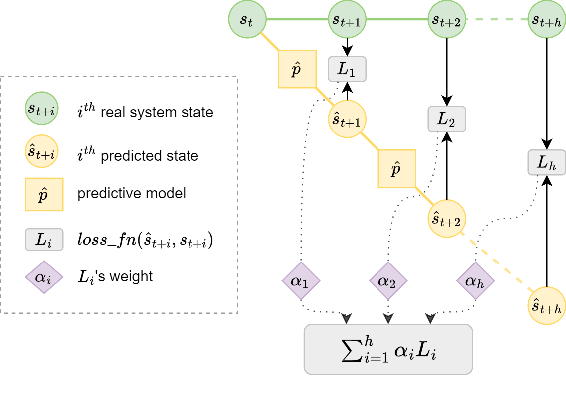
Figure 1: Schematic representation of the multi-step prediction framework using a one-step predictive model $\hat{p}$. The diagram illustrates the iterative prediction of future states $\hat{s}_{t+i}$, the computation of per-horizon losses $L_{i}$ against real system states $s_{t+1}$, and the weighting of these losses $\alpha_{i}$ to optimize the predictive model over a horizon of $h$ steps.

MBRL algorithms alternate between two steps: i) model learning, a supervised learning problem to learn the dynamics of the environment, and ii) policy optimization, where a policy and/or a value function is updated by sampling from the learned dynamics. MBRL is recognized for its sample efficiency, as policy/value learning is conducted (either wholly or partially) from imaginary model rollouts (also referred to as background planning), which are more cost-effective and readily available than rollouts in the true dynamics (Janner et al., 2019). Moreover, a predictive model that performs well out-of-distribution facilitates easy transfer to new tasks or areas not included in the model training dataset (Yu et al., 2020).

While MBRL algorithms have achieved significant success, they are prone to compounding errors when planning over extended horizons (Lambert et al., 2022). This issue arises due to the propagation of one-step errors, leading to highly inaccurate predictions at longer horizons. This can be problematic in real-world applications, as it can result in out-of-distribution states that may violate the physical constraints of the environment, and misguide planning. The root of compounding errors is in the nature of the models used in MBRL. Typically, these are one-step models that predict the next state based on the current state and executed action. Long rollouts are then generated by iteratively applying these models, leading to compounding errors. To tackle this problem, our approach involves adjusting the training objective of these models to focus on optimizing for long-horizon error (Figure 1). This strategy is especially beneficial in presence of additive noise in observations, a context that mirrors real-world scenarios. Indeed, in situations where state perturbations occur due to unavoidable measurement errors or adversarial attacks (Zhang et al., 2021; Sun et al., 2023), aiming to minimize the long-horizon error is advantageous. It enhances the signal-to-noise ratio by incorporating future information, thereby improving the practical effectiveness of the models.

Our key contributions are the following.

• We propose a novel training objective for one-step predictive models consisting in a weighted sum of MSE (Mean Squared Error) losses at several future horizons.

• We use two tractable cases to demonstrate the advantages of our weighted multi-step loss. In a linear system, this loss allows for the identification of minimizers achieving a bias-variance trade-off. In the case of a two-parameter neural network, we show how important the weights are to achieve strong performance across multiple future horizons.

• Finally, we analyze the optimal weight configurations of the multi-step loss and show that models trained with this loss improves over the one-step baseline across diverse environments, datasets, and levels of noise.

2 Preliminaries

The conventional framework used in RL is the finite-horizon Markov decision process (MDP), defined by the tuple $\mathcal{M}=\langle\mathcal{S},\mathcal{A},p,r,\rho_{0},\gamma\rangle$. In this notation, $\mathcal{S}$ is the state space and $\mathcal{A}$ is the action space. The transition dynamics, which could be stochastic, are represented by $p:\mathcal{S}\times\mathcal{A}\leadsto\mathcal{S}$. The reward function is denoted by $r:\mathcal{S}\times\mathcal{A}\rightarrow\mathbb{R}$. The initial state distribution is given by $\rho_{0}$, and the discount factor is represented by $\gamma\in(0,1]$. The objective of RL is to identify a policy $\pi:\mathcal{S}\leadsto\mathcal{A}$. This policy aims at maximizing the expected sum of discounted rewards, denoted as $J(\pi,\mathcal{M}):=\mathbb{E}_{s_{0}\sim\rho_{0},a_{t}\sim\pi,\,s_{t>0}\sim p}[\sum_{t=0}^{H}\gamma^{t}r(s_{t},a_{t})]$, where $H$ represents the horizon of the MDP.

Model-based RL (MBRL) algorithms learn a model of the dynamics of the environment $\hat{p}$ (and sometimes of the reward function $\hat{r}$ as well) in a supervised fashion from data collected when interacting with the real system $p$. The loss function is typically the negative log-likelihood $\mathcal{L}(\mathcal{D};\hat{p})=-\frac{1}{N}\sum_{i=1}^{N}\log\hat{p}(s^{i}_{t+1}|s^{i}_{t},a^{i}_{t})$ for stochastic models or mean squared error (MSE) in the case of deterministic ones. The learned model can subsequently be employed for policy search under the MDP $\widehat{\mathcal{M}}=\langle\mathcal{S},\mathcal{A},\hat{p},r,\rho_{0},\gamma\rangle$. This MDP shares the state and action spaces $\mathcal{S},\mathcal{A}$, and the reward function $r$, with the true MDP $\mathcal{M}$, but uses the dynamics $\hat{p}$ learned from the dataset $\mathcal{D}$. The policy $\hat{\pi}=\mathop{\rm argmax}_{\pi}J(\pi,\widehat{\mathcal{M}})$ learned on $\widehat{\mathcal{M}}$ is not guaranteed to be optimal under $\mathcal{M}$ due to distribution shift and model error.

In this work, we also consider state-perturbed MDPs that fall under the formalism of partially-observed Markov decision process (POMDP). Indeed, a POMDP is defined by the underlying MDP $\langle\mathcal{S},\mathcal{A},p,r,\rho_{0},\gamma\rangle$, in addition to a set of possible observations $\Omega$, and an observation function $f_{o}:\mathcal{S}\times\mathcal{A}\leadsto\Omega$ ( where $o_{t}\sim f_{o}(\cdot|a_{t-1},s_{t})$). In practice, we consider systems with additive Gaussian noise in observations $o_{t}=s_{t}+\epsilon$ where $\epsilon\sim{\cal N}(0,\Sigma)$, which is a special case of a POMDP. This formalism is closely related to state-noisy MDPs (Sun et al., 2023) and state-adversarial MDPs (Zhang et al., 2021) where an attacker engineers the perturbation to intentionally decrease the performance of solvers.

The formal definition of the multi-step loss is given in Section 3. We then present the related work in Section 4. We study the properties of the multi-step loss in Section 5. This is done through two tractable cases: a uni-dimensional linear system in and a two-parameter non-linear system. Finally, the experimental setup and the performance evaluation of the models is discussed in Section 6.

3 The multi-step loss

In MBRL, it is common to use a parametric model $\hat{p}_{\theta}$ that predicts the state one-step ahead $\hat{s}_{t+1}\mathrel{\text{\reflectbox{\char 59\relax}}}\hat{p}_{\theta}(s_{t},a_{t})$. We train this model to optimize the one-step predictive error $L\big{(}s_{t+1},\hat{p}_{\theta}(s_{t},a_{t})\big{)}$ (MSE or NLL for stochastic modeling) in a supervised learning setting. To learn a policy, we use these models for predicting $h$ steps ahead by applying a procedure called rollout.

Definition 3.1.

(Rollout). We generate $\hat{s}_{t+j}\mathrel{\text{\reflectbox{\char 59\relax}}}\hat{p}_{\theta}(\hat{s}_{t+j-1},a_{t+j-1})$ recursively for $j=1,\ldots,h$, to collect a trajectory $\tau=(s_{0},a_{0},\hat{s}_{1},a_{1},...,\hat{s}_{j},a_{j},...)$, where $(a_{t},\ldots,a_{t+h-1})={\bm{a}}_{t:t+h-1}={\bm{a}}_{\tau}$ is either a fixed action sequence generated by planning or sampled from a policy $a_{t+j}\mathrel{\text{\reflectbox{\char 59\relax}}}\pi(s_{t+j})$ for $j=1,\ldots,h$, on the fly.

Formally, let

$$\hat{s}_{t} =s_{t}$$

$$\hat{s}_{t+j-1} \mathrel{\text{\reflectbox{\char 59\relax}}}\hat{p}_{\theta}(\hat{s}_{t+j-2},a_{t+j-2})$$

$$\hat{p}_{\theta}^{j}(s_{t},{\bm{a}}_{t:t+j-1}) =\hat{p}_{\theta}\big{(}\hat{s}_{t+j-1},a_{t+j-1}\big{)}\hskip 5.69046pt\text{ for }j=1,\ldots,h$$

Using $\hat{p}_{\theta}^{h}(s_{t},{\bm{a}}_{t:t+h-1})$ to estimate $s_{t+h}$ is problematic for two reasons:

• A distribution mismatch occurs between the inputs that the model was trained on ($s_{t+1}\mathrel{\text{\reflectbox{\char 59\relax}}}p(s_{t},a_{t})$) and the inputs the model is being evaluated on ($\hat{s}_{t+1}\mathrel{\text{\reflectbox{\char 59\relax}}}\hat{p}_{\theta}(s_{t},a_{t})$Talvitie (2014; 2017).

• The predictive error (and the modeled uncertainty in the case of stochastic models) will propagate through the successive model calls, leading to compounding errors (Lambert et al., 2022; Talvitie, 2014; Venkatraman et al., 2015).

To mitigate these issues, we study models that, given the full action sequence ${\bm{a}}_{t:t+h-1}$, learn to predict the state $s_{t+h}$ by recursively predicting the intermediate states $s_{t+j}$, for $j=1,\ldots,h$. We address this problem through the use of a weighted multi-step loss that accounts for the predictive error at different future horizons.

Definition 3.2.

(Weighted multi-step loss). Given horizon-dependent weights ${\bm{\alpha}}=(\alpha_{1},\ldots,\alpha_{h})$ with $\sum_{i=1}^{h}\alpha_{i}=1$, a one-step loss function $L$, an initial state $s_{t}$, an action sequence ${\bm{a}}_{\tau}={\bm{a}}_{t:t+h-1}$, and the real (ground truth) visited states ${\bm{s}}_{\tau}={\bm{s}}_{t+1:t+h}$, we define the weighted multi-step loss as

$$L^{h}_{\bm{\alpha}}\big{(}{\bm{s}}_{\tau},\hat{p}_{\theta}(s_{t},{\bm{a}}_{\tau})\big{)}=\\ \sum_{j=1}^{h}\alpha_{j}L\big{(}s_{t+j},\hat{p}_{\theta}^{j}(s_{t},{\bm{a}}_{t:t+j-1})\big{)}.$$

The dependency of $L^{h}_{\bm{\alpha}}$ on $h$ is omitted in the rest of the paper when $h$ is clear from the context. Furthermore, the loss $L$ used in the multi-step loss $L_{\bm{\alpha}}$ will always be the MSE.

Algorithm 1 shows the training procedure of multi-step models. We emphasize that unlike popular methods in the existing literature (teacher forcing (Williams & Zipser, 1989), hallucinated replay Talvitie (2014) and data-as-demonstrator Venkatraman et al. (2015)), which consists in augmenting the training data with predicted states, our method consists in back-propagating the gradient of the loss through the successive compositions of the model $\hat{p}_{\theta}$ figuring in $L_{\bm{\alpha}}$.

Algorithm 1 Training a model using the multi-step loss

  Input: model $\hat{p}_{\theta}$, trajectory $\tau=(s_{t+i},a_{t+i})_{i=0}^{h}$, loss function $L$, horizon $h$, normalized weights $\{\alpha_{i}\}_{i=1}^{h}$

  Initialize the loss $l=0$

  $s=s_{t}$

  for $i=0$ to $h-1$ do

     Sample from the model $\hat{s}_{t+i+1}\mathrel{\text{\reflectbox{\char 59\relax}}}\hat{p}_{\theta}(s,a_{t+i})$

     Update the loss $l\mathrel{+}=\alpha_{i}\cdot L(\hat{s}_{t+i+1},s_{t+i+1})$

     $s=\hat{s}_{t+i+1}$

  end for

  Update $\theta$ using a gradient step minimizing $l$

4 Related Work

The premises of multi-step dynamics modeling can be tracked back to early work about temporal abstraction (Sutton et al., 1999; Precup et al., 1998) and mixture of timescale models in tabular MDPs (Precup & Sutton, 1997; Singh, 1992; Sutton & Pinette, 1985; Sutton, 1995). These works study fixed-horizon models that learn an abstract dynamics mapping from initial states to the states $j$ steps ahead. A different approach consists in optimizing the multi-step prediction error of single-step models that are used recursively, which we study here. This approach has been studied for recurrent neural networks (RNNs) and is referred to as teacher forcing (Lamb et al., 2016; Bengio et al., 2015; Huszár, 2015; Pineda, 1988; Williams & Zipser, 1989). The idea consists in augmenting the training data with predicted states. More recent works have built on this idea (Abbeel et al., 2005; Talvitie, 2014; 2017; Venkatraman et al., 2015). These methods, albeit optimizing for future prediction errors, assume the independence of the intermediate predictions on the model parameters, making them more of a data augmentation technique than a proper optimization of multi-step errors.

The closest works to ours which also consider the intermediate predictions to be dependent on the model parameters are Lutter et al. (2021), Byravan et al. (2021) and Xu et al. (2018). These works all use an equally-weighted multi-step loss whereas we emphasize on the need of having a weighted multi-step loss. Nagabandi et al. (2018) only use an equally-weighted multi-step loss for validation, which is also common in the time series literature (Tanaka et al., 1995; Fraedrich & Rückert, 1998; McNames, 2002; Ben Taieb & Bontempi, 2012; Ben Taieb et al., 2012; Chandra et al., 2021). Lutter et al. (2021) and Xu et al. (2018) find that only small horizons ($h=2,3,5$) yield an improvement over the baseline, which we suggest is due to using equal weights in the multi-step loss. Byravan et al. (2021) successfully use $h=10$ with equal weights in the context of model-predictive control (MPC). However, they consider it as a fixed design choice and might have tailored their approach accordingly. To the best of our knowledge we are the first work highlighting the importance of the weighting mechanism in balancing the multi-step errors. Futhermore, we particularly stress the importance of having a weighted multi-step loss for state-noisy MDPs and study the impact of the noise level. We believed that such a setting is still under-studied event though previous model-free methods have been proposed (Hess et al., 2023; Sun et al., 2023; Zhang et al., 2021; Pattanaik et al., 2017) and a very recent work (Noa, 2023) presents a model-based approach using diffusion models.

5 Understanding the multi-step loss: two case studies

5.1 Uni-dimensional linear system

The first case consists in studying the solutions of the multi-step loss for $h=2$ in the case of an uncontrolled linear (discrete) dynamical system with additive Gaussian noise, and a linear model. With such a simple formulation, we benefit from the fact that the optimization is tractable and closed-form solutions can be obtained for each ${\bm{\alpha}}\in[0,1]$. We start by defining the system and the model.

Definition 5.1.

(Uni-dimensional linear system with additive Gaussian noise). For an initial state $s_{0}\in{\mathbb{R}}$ and an unknown parameter $\theta_{true}\in(-1,1)$ (for stability) we define the transition function and observations as

$$s_{t+1} =\theta_{true}\cdot s_{t}$$

$$o_{t+1} =s_{t+1}+\epsilon_{t+1}\text{ with }\epsilon_{t+1}\sim{\cal N}(0,\sigma^{2})\text{ and }\sigma\in{\mathbb{R}}$$

Definition 5.2.

(Linear model). For an initial state $s_{0}\in{\mathbb{R}}$ and a parameter $\theta\in{\mathbb{R}}$ that we learn by minimizing the multi-step loss for $h=2$, we define the linear model as $\hat{s}_{t+1}=\hat{p}_{\theta}(s_{t})=\theta\cdot s_{t}$

In this setup, the multi-step loss for $h=2$ boils down to a polynomial in the model’s parameter $\theta$:

$$L_{\alpha}\big{(}{\bm{o}}_{\tau},\hat{p}_{\theta}(s_{t})\big{)}=\\ \alpha(\theta s_{t}-o_{t+1})^{2}+(1-\alpha)(\theta^{2}s_{t}-o_{t+2})^{2}$$

where ${\bm{o}}_{\tau}=(o_{t+1},o_{t+2})$. The aim of our study is to analyze the statistical properties of $\hat{\theta}(\alpha)\in\mathop{\rm argmin}_{\theta}L_{\alpha}\big{(}{\bm{o}}_{\tau},\hat{p}_{\theta}(s_{t})\big{)}$ for different values of $\alpha$ and different values of the observational noise scale $\sigma$.

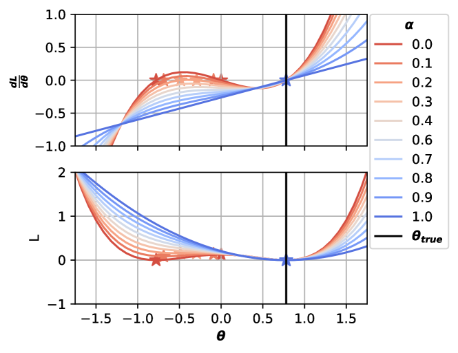
Figure 2: The loss function and its derivative for different values of $\theta$ and $\alpha$, in absence of noise ($\sigma=0$). In this figure, $\theta_{true}$ is fixed to a randomly selected value, $\theta_{true}=0.78$. The roots of the derivative are highlighted with stars.

Figure 2 shows the loss function curve and its critical points for different values of $\alpha$. The minimizers $\hat{\theta}(\alpha)$ can be obtained by solving the polynomial equation $dL_{\alpha}/d\theta=0$. When $\alpha\in(0,1)$, we compute the roots of the cubic polynomial equation using Cardano’s formulas. These latter include at least one real root ($\alpha\geq 0.3$ in Figure 2) and two (potentially real) conjugate complex roots ($\alpha<0.3$ in Figure 2).

In the rest of the experiments, we fix a dataset of initial states ${\cal S}_{0}$ and sample $K$ times a two-step transition, yielding a dataset ${\cal D}={({\cal S}_{0},{\cal O}^{j}_{1},{\cal O}^{j}_{2})_{j=1,\ldots,K}}$. This dataset showcases different realizations of the observational noise, which is sampled i.i.d. from a Gaussian distribution ${\cal N}(0,\sigma^{2})$.

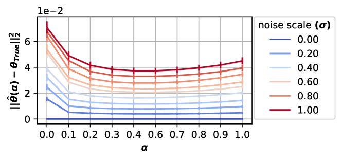
Figure 3: The distance between the true parameters and the optimal parameters for different values of $\alpha$ and noise scales.

We then compare the distance between the minimizers of the loss function with different values of $\alpha$ and the true parameter $\theta_{true}$. When there is more than one root, we assume access to the sign of $\theta_{true}$ so that we can choose the correct estimator $\hat{\theta}(\alpha)$. Figure 3 shows that as the noise increases, the vanilla MSE loss estimator ($\alpha=1$) is not the best estimator with respect to the distance to the true parameter $\theta_{true}$. Interestingly, the best solution is obtained for $\alpha\in(0,1)$.

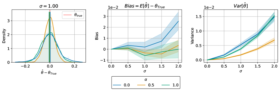
Figure 4: The left panel shows the density distribution of $\hat{\theta}-\theta_{true}$ for a fixed $\sigma$ of 1.0. The middle panel delineates the bias of the estimator, defined as $E[\hat{\theta}]-\theta_{true}$, across varying levels of $\sigma$, and weights $\alpha\in\{0,0.5,1\}$ indicated by color. The right panel presents the variance of the estimator, $Var[\hat{\theta}]$, as a function of $\sigma$ for the same set of $\alpha$ values. The shaded regions represent the 95% bootstrap confidence intervals across ten $\theta_{true}$ values and 100 Monte Carlo simulations.

To understand the observed results, we compute the closed-form solutions of the multi-step loss in the case of $\alpha=0$ and $\alpha=1$:

Proposition 5.3.

($\alpha=1$). Given a transition $(s_{t}\neq 0,o_{t+1})$ from the linear system and a linear model with parameter $\theta$, the minimizer of the $\alpha=1$ multi-step loss can be computed as:

$$\hat{\theta}_{1}=\frac{o_{t+1}}{s_{t}}=\theta_{true}+\frac{\epsilon_{t+1}}{s_{t}}$$

Proposition 5.4.

($\alpha=0$). Given a transition $(s_{t}\neq 0,o_{t+1},o_{t+2})$ from the linear system, a linear model with parameter $\theta$, the sign of the true parameter (for instance $\theta_{true}>0$), and assuming its existence ($\frac{o_{t+2}}{s_{t}}>0$), the minimizer of the $\alpha=0$ multi-step MSE loss can be computed as:

$$\hat{\theta}_{0}=\sqrt{\frac{o_{t+2}}{s_{t}}}=\sqrt{\theta_{true}^{2}+\frac{\epsilon_{t+2}}{s_{t}}}$$

Remark 5.5.

For ease of notation in Proposition 5.3 and Proposition 5.4, we compute the solutions given only one transition $(s_{t},o_{t+1},o_{t+2})$. In practice, one minimizes the empirical risk based on a training dataset of size $N$: ${\cal D}=\{(s_{i,t},o_{i,t+1},o_{i,t+2})\}_{i=1:N}$, in which case the closed-form solutions become:

$$\begin{cases}\hat{\theta}_{1}=\theta_{true}+\frac{\sum_{i=1}^{N}\epsilon_{i,t+1}}{\sum_{i=1}^{N}s_{i,t}}\\ \hat{\theta}_{0}=\sqrt{\theta_{true}^{2}+\frac{\sum_{i=1}^{N}\epsilon_{i,t+2}s_{i,t}}{\sum_{i=1}^{N}s_{i,t}^{2}}}\end{cases}$$

On the one hand, we observe that while $\hat{\theta}_{1}$ is an unbiased estimator of $\theta_{true}$ ($E_{\epsilon_{t+1}\sim{\cal N}(0,\sigma^{2})}[\hat{\theta}_{1}]=\theta_{true}$), its variance grows linearly with the noise scale: ${\rm Var}_{\epsilon_{t+1}\sim{\cal N}(0,\sigma^{2})}[\hat{\theta}_{1}]=\frac{\sigma^{2}}{s_{t}^{2}}$. On the other hand, $\hat{\theta}_{0}$ is a potentially biased estimator, but with a smaller variance if $\theta_{true}\gg 1$ ($\frac{\epsilon_{t+2}}{4\theta_{true}^{2}s_{t}^{2}}\approx 0$). In this case we can use a first-order Taylor expansion to approximate ${\rm Var}[\hat{\theta}_{0}]={\rm Var}_{\epsilon_{t+2}\sim{\cal N}(0,\sigma^{2})}[\hat{\theta}_{0}]$:

$${\rm Var}[\hat{\theta}_{0}] ={\rm Var}\big{[}\sqrt{\theta_{true}^{2}+\frac{\epsilon_{t+2}}{s_{t}}}\big{]}$$

$$\approx\theta_{true}^{2}{\rm Var}\big{[}1+\frac{\epsilon_{t+2}}{2\theta_{true}^{2}s_{t}}\big{]}=\frac{\sigma^{2}}{4\theta_{true}^{2}s_{t}^{2}}$$

$$\leq{\rm Var}[\hat{\theta}_{1}]$$

For intermediate models ($\alpha\in(0,1)$), and in general when the conditions of the last result do not necessarily hold, we use Monte Carlo simulations to compare the variance of $\hat{\theta}_{\alpha\in\{0,0.5,1\}}$. Figure 4 shows the variance reduction brought by the multi-step loss when $\alpha=0.5$. It is also noticeable that, up to the noise scales considered in this experiment, $\alpha=0$ generates a large bias (which matches the theoretical insights), while no significant bias is observed for the estimator with $\alpha=0.5$. We conclude that in the case of a noisy linear system, the multi-step MSE loss minimizer with $\alpha=0.5$ is a statistical estimator that (empirically) has a smaller variance and a comparable bias to the one-step loss minimizer. It is worth noticing that when the noise is non-zero the best solution for the one-step MSE is obtained for $\alpha\in(0,1)$ and not $\alpha=1$ (which corresponds to optimizing exactly the one-step MSE).

In this linear case, we had access to closed-form solutions. However, Figure 2 shows that choosing the multi-step MSE loss as an optimization objective introduces additional critical points where a gradient-based optimization algorithm might get stuck. We now empirically study the optimization process in the case of a two-parameter neural network.

5.2 Two-parameter non-linear system

As an attempt to get closer to a realistic MBRL setup where neural networks are used for dynamics learning, we study a non-linear dynamical system using a two-parameters neural network model:

Definition 5.6.

(Two-parameter non-linear system with additive Gaussian noise). For an initial state $s_{0}\in{\mathbb{R}}$ and unknown parameters ${\bm{\theta}}^{true}=(\theta_{1}^{true},\theta_{2}^{true})\in{\mathbb{R}}^{2}$ we define the transition function and observations as

$$s_{t+1} =\theta_{1}^{true}\cdot sigmoid(\theta_{2}^{true}\cdot s_{t})$$

$$o_{t+1} =s_{t+1}+\epsilon_{t+1}\text{ with }\epsilon_{t+1}\mathrel{\text{\reflectbox{\char 59\relax}}}{\cal N}(0,\sigma^{2})\text{ and }\sigma\in{\mathbb{R}}$$

Definition 5.7.

(Two-parameters neural network model). A single-neuron two-layer (without bias) neural network. We denote its parameters ${\bm{\theta}}=(\theta_{1},\theta_{2})\in{\mathbb{R}}^{2}$:

$$\hat{s}_{t+1} =\hat{p}(s_{t})=\theta_{1}\cdot sigmoid(\theta_{2}\cdot s_{t})$$

To get a broader idea about the optimization challenges in this setup, we show the loss landscape for different values of $\alpha$ and noise scales $\sigma$ in Section D.2.1. Regarding the gradient-based optimization, we compare the solution reached after training in terms of the one-step and two-step validation MSE losses (the details of the experiment are given in Section D.2.2).

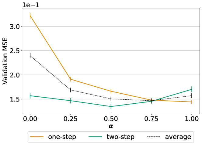
Figure 5: The validation one-step MSE $L_{1}$ (in yellow), the validation two-step MSE $L_{0}$ (in green) and the average of these two MSEs (dashed black line) for different values of $\alpha$. The error bars represent the 95% bootstrap confidence intervals across 2 optimizers, 3 initialization distributions, 10 initial points, 3 noise levels, and 10 Monte Carlo simulations.

Figure 5 shows that even in the presence of noise, compared to the linear case, the best value of $\alpha$ for the one-step MSE is $\alpha=1$. This can be explained by the use of lower levels of noise in the simulations than the linear case. The intermediate models obtained for $\alpha\in\{0.25,0.5,0.75\}$ represent a trade-off between the one-step and two-step MSEs. The average of the two MSEs, which we use in the experiment section to assess the overall quality of our models over a range of horizons, achieves its minimum for $\alpha=0.75$. Notice that the validation losses are only used for evaluation, and do not match the training loss which depends on $\alpha$.

6 Experiments & results

In this section, we evaluate the performance of models trained with the multi-step loss $L_{{\bm{\alpha}}}$ for different values of the horizon $h$ and different noise levels of the dynamics. We first describe the multi-step loss hyperparameters: the horizon $h$ and the weights ${\bm{\alpha}}$. For the evaluation of the models we consider both a static and a dynamic setup. The static evaluation denotes the evaluation of dynamics models in terms of predictive error in held-out test datasets. For the dynamic evaluation we will consider the offline MBRL setting (Levine et al., 2020) where the goal is to learn a policy from a given dataset without interacting further with the environment. The evaluation is done on three classical RL environments (Cartpole swing-up, Swimmer and Halfcheetah) and various datasets (eight in total) collected with different behavior policies (random, medium, full_replay and mixed_replay) on these environments. The details of these tasks are provided in Appendix A. For all these tasks, we use the same neural network model for $\hat{p}_{\theta}$. Implementation details for the model are given in Appendix B.

6.1 Hyperparameters of the multi-step loss

The multi-step loss depends on the following hyperparameters: the loss horizon $h$ and the corresponding weights $\{\alpha_{i}\}_{i=1}^{h}$.

6.1.1 The horizon $h$

The horizon of the loss is the maximal prediction horizon considered in the loss. Typically, in this paper we consider $h\in\{2,3,4,10\}$ for the multi-step loss and $h=1$ for the single-step baseline.

6.1.2 The weights $\alpha$

For a horizon $h$, the weights ${\bm{\alpha}}$ live in the $(h-1)$-dimensional probability simplex, which means that the search space is $(0,1)^{h-1}$. As the MSE has been shown to grow exponentially with the horizon when applying one-step models recursively (Theorem 1 of Venkatraman et al. (2015)) we choose an exponentially parameterized profile for the weights. The objective is to give each MSE term the same importance when we optimize the MSE loss. Given a weighted multi-step loss $L_{\bm{\alpha}}$ with horizon $h$, weights ${\bm{\alpha}}$, and $\beta>0$, the exponentially parameterized weights are defined as:

$$\alpha_{i}=\underbrace{(\frac{1-\beta}{1-\beta^{h+1}})}_{\text{normalization constant}}\cdot\beta^{i}\hskip 8.5359pt\text{for }i\in\{1,\ldots,h\}.$$

Applying this exponential parametrization of the weights, we further reduce the search space dimension. In our experiments, we still consider values greater than 1 in the grid, values corresponding to an increase of the weights over the horizon. This approach is used to analyze whether certain settings would benefit from focusing on large horizons.

6.2 Static evaluation with the R2 metric

The commonly used metrics for the static evaluation are the standard mean squared error (MSE) or the explained variance (R2) which we prefer over the MSE because it is normalized and can be aggregated over multiple dimensions. In our attempt to reduce compounding errors in MBRL, we are especially interested in the long-term predictive error of models. For each horizon $h$, the error is computed by considering all the sub-trajectories of size $h$ from the test dataset. The predictions are computed by calling the model recursively $h$ times (using the ground truth actions of the sub-trajectories) and the average R2 score at horizon $h$, $\text{R2}(h)$, averaged over the sub-trajectories is reported: given a dataset ${\cal D}=\{(s_{i,t},a_{i,t},s_{i,t+1},\ldots)\}_{i=1,\ldots,N}$, a predictive model $\hat{p}_{\theta}$, for $h=1,\ldots,H$:

$$\text{R2}(h)=\frac{1}{d_{s}}\sum_{j=1}^{d_{s}}1-\frac{\frac{1}{N}\sum_{i=1}^{N}\left(s^{j}_{i,t+h}-\hat{p}_{\theta}^{h}(s_{i,t},{\bm{a}}_{i,t:t+h})^{j}\right)^{2}}{\frac{1}{N}\sum_{i=1}^{N}\left(s^{j}_{i,t+h}-\bar{s}^{j}_{t+h}\right)^{2}}.$$

We also report the average R2 score, $\overline{R2}(H)$, over all prediction horizons from $1$ to $H$.

$$\overline{R2}(H)=\frac{1}{H}\sum_{h=1}^{H}\text{R2}(h).$$

For the weights of the loss we perform a grid search over $\beta$ values, selecting the value giving the best $\overline{R2}(H)$ averaged over 3 cross-validation folds.

Figure 6: The series of bar plots display the relative improvement with respect to the $h=1$ baseline, in the test $\overline{R2}(50)$ metric for various environments, and datasets. Performance is evaluated over loss horizons $h$ with the relative improvement measured on a logarithmic scale. The relative noise scale, ranging from 0.0 to 0.05, is color-coded and represents a ratio of the range of the state space, for each dataset. The error bars indicate the 95% confidence intervals ($\text{mean}\pm 1.96\cdot\text{standard error}$) obtained with the three cross-validation folds.

Figure 6 shows the relative improvement in percentage over the one-step model of the $\overline{R2}(50)$ metric for the different datasets (the absolute values of the metric and the full $R2(h)$ curves are shown in Section D.3). For most of the datasets (all the Cartpole and Swimmer datasets, and Halfcheetah random and medium_replay) the benefit of using the multi-step loss when there is noise is clear and for most of them (all the Cartpole datasets, Swimmer random and Halfcheetah random) the larger the noise the higher the benefit. The impact of the horizon $h$ of the loss is less clear although for some datasets increasing the horizon $h$ as the noise increases also helps. This result is more mitigated on Halfcheetah medium which we suggest is due to the optimization process converging to sub-optimal solutions. We also note that even if the multi-step loss is using $h=10$, because of the weights, the multi-step loss could finally be close to the multi-step losses obtained with $h=2$, 3 or 4, which would mean that a smaller horizon is sufficient. This is an advantage of our flexible multi-step loss that can adapt its horizon thanks to the selection of the best weights

We now study the best weights obtained for each multi-step loss ($h=2$, 3, 4, and 10) and each noise scale. First, we observe from Table 1 that compared to what is usually done in the literature, the best weights are not uniform. Second, we also notice an increase of the parameter $\beta$ with the noise scale. This finding supports the idea that multi-step models are increasingly needed when incorporating information from the future is crucial to achieve better performance. We also discuss the effective horizon obtained with the weights in Section D.3.2.

Table 1: Best $\beta$ values found with a grid search for each horizon and each noise scale. The values are averaged over the eight datasets.

	horizon $h$
	2	3	4	10
$\sigma$ (%)	$\beta$
0	0.81	0.45	0.41	0.46
1	0.56	0.76	0.51	0.47
2	0.86	0.72	0.78	0.54
3	0.67	1.21	0.81	0.50
4	0.74	1.01	0.74	0.55
5	1.33	0.83	0.97	0.51

6.3 Dynamic evaluation: offline MBRL

We consider the offline setting where given a set of $N$ trajectories $\mathcal{D}=\{(s_{t}^{i},a_{t}^{i},s_{t+1}^{i},\ldots)\}_{i=1}^{N}$, the goal is to learn a policy maximizing the return in a single shot, without further interacting with the environment.

We consider a Dyna-style agent that learns a parametric model of the policy based on data generated from the learned dynamics model $\hat{p}_{\theta}$. Specifically, we train a Soft Actor-Critic (SAC) (Haarnoja et al., 2018) with short rollouts on the model a la MBPO Janner et al. (2019), a popular MBRL algorithm. We then rely on model predictive control (MPC) at decision-time where the action search is guided by the SAC policy. The details of this agent are given in Section A.3.

The experiments are run on the Cartpole mixed_replay dataset without noise (noise scale of $1\%$). The reason is that the range of episode returns spanned by this dataset makes us hope that it is possible to learn a model that is good enough to learn a successful policy (for which episode returns are higher than 800). The distribution of the returns on the random and full replay datasets makes it more challenging to learn a successful policy. The goal here is not to study a new offline MBRL algorithm, avoiding unknown regions of the state-action space, but studying the improvement that can be obtained with the multi-step loss when varying the horizon $h$. Finally, in order to isolate the effect of dynamics learning, we assume that the reward function is a known deterministic function of the observations.

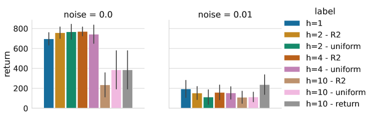
Figure 7: Returns of the agents trained on multi-step models in the Cartpole mixed_replay task. The error bars indicate the 95% confidence intervals ($\text{mean}\pm 1.96\cdot\text{standard error}$).

As it is acknowledged that static evaluation metrics may not always align with the final return of agents (see for instance (Lambert et al., 2021)) we also include the performance of the models trained on the 10-step loss with weights tuned to maximize the return, using the same grid search as for the R2.

Without noise.

Figure 7 shows the return obtained by the different models on the Cartpole mixed_replay task. Against a strong baseline ($h=1$) with a near 700 return, it is observed that the multi-step models exhibit marginally superior performance, especially for $h$ values of 2 and 4. However, this trend is not maintained for $h=10$, indicating that larger horizons may not be beneficial in this context. Additionally, the study compares these outcomes with those obtained using uniform weights, a common approach in most related research. As depicted in Figure 7, the returns for uniform weight variants at $h$ values of 2 and 4 are comparable to those of the models selected based on the $\overline{R2}(50)$ metric. While uniform weights help the $h=10$ model reach a better return, it remains sub-optimal with respect to the baseline. These findings confirm a common result in the literature (Lutter et al., 2021; Xu et al., 2018), stating that the multi-step loss is only useful for small values of $h$.

With noise.

In the presence of noise, we observe that the performance of all models, including the baseline, significantly decreases. Notably, the optimal multi-step models do not demonstrate any improvement in this setting, a finding that also holds true for the variant with uniform weights. We found that $\beta=0.3$ maximizes the return for the 10-step loss and leads to a marginal improvement over the baseline model. This finding challenges the common practice of using uniform weights in related research, suggesting that a more tailored approach is necessary for each specific task. We believe that a better hyperparameter search for the multi-step loss weights could lead to better performance of the corresponding multi-step models.

7 Conclusion

In this paper, we introduce a weighted multi-step loss that leads to models exhibiting significant improvements in the average R2 score over future horizons in various datasets derived from popular RL environments with noisy dynamics. These outcomes align with our analysis of two tractable scenarios: models optimized for the multi-step loss outperform those focused on minimizing the one-step loss in the presence of noise. The insights from dynamic evaluation present a more complex picture. Specifically, we found that in absence of noise, the multi-step loss slightly improved the return of an already strong one-step baseline. However, a noticeable improvement in the noisy scenario would require an extensive search for optimal hyperparameters, including the weights and, implicitly, the prediction horizon.

Appendix

Appendix A The evaluation setup

A.1 Environments

Figure 10: The environments: Cartpole swing-up, Swimmer and Halfcheetah.

In the present study, we examine three distinct environments within the scope of continuous control reinforcement learning, as delineated in Figure 10, each exhibiting varying degrees of complexity. The complexity of a given environment is primarily determined by the dimension of the state space $d_{s}$, and the dimension of the action space $d_{a}$. Notably, Cartpole swing-up is a classic problem in the field where the task is to swing up a pole starting downwards, and balance it upright. The other considered tasks are Swimmer and Halfcheetah, which are two locomotion tasks, aiming at maximizing the velocity of a virtual robot along a given axis. Swimmer incorporates fluid dynamics with the goal of learning an agent that controls a multi-jointed snake moving through water. On the other hand, Halfcheetah simulates a two-leg Cheetah with the goal of making it run as fast as possible. For the latter environments, we use the implementation of OpenAI Gym (Brockman et al., 2016), and the implementation of Deepmind Control (Tassa et al., 2018) for Cartpole. Both libraries are based on the Mujoco physics simulator (Todorov et al., 2012). A detailed description of these environments is provided in Table 2.

Table 2: The environments characteristics. $d_{s}$: the dimension of the state space, $d_{a}$: the dimension of the action space, $x_{t}$: position along the $x$-axis, $\dot{x}_{t}$: velocity along the $x$-axis, $\|a_{t}\|_{2}^{2}$: the action $a_{t}$ magnitude, $\theta$: the angle of the pole (only for Cartpole).

environment	$d_{s}$	$d_{a}$	task horizon	reward function
Cartpole swing-up	5	1	1000	$\frac{1+\cos\theta_{t}}{2}\times\frac{1+e^{-0.25\log(10)x_{t}^{2}}}{2}\times\left(1-\frac{a_{t}^{2}}{5}\right)\times\frac{1+e^{-0.04\log(10){\dot{x}_{t}}^{2}}}{2}$
Swimmer	8	2	1000	$\dot{x}_{t}-0.0001\times\|a_{t}\|_{2}^{2}$
Halfcheetah	17	6	1000	$\dot{x}_{t}-0.1\times\|a_{t}\|_{2}^{2}$

A.2 Datasets

In this section, we introduce the different datasets that are used to evaluate the multi-step models. These datasets are collected using some behavior policies that are unknown to the models.

Table 3 illustrates the features of datasets across the three environments: Cartpole Swing-up, Swimmer, and Halfcheetah. These environments vary in dataset size and behavioral policies. In the Cartpole Swing-up setting, each of the three datasets (random, mixed_replay, and full_replay) includes 50 episodes, which are split into training, validation, and testing subsets. The and full_replay depict complete learning trajectories of an unstable model and a state-of-the-art (sota) model-based Soft Actor-Critic (SAC) respectively (Janner et al., 2019), and integrated with shooting-based planning Section A.3. For the Swimmer environment, both the random and full_replay datasets consist of 50 episodes each. The random dataset is derived from a random policy, whereas the full_replay dataset is generated using a model-based SAC with planning. For both the Cartpole Swing-up and Swimmer environments, the datasets were self-collected due to the absence of a unified benchmark that includes datasets from both tasks.

Table 3: The datasets characteristics. mf: model-free, mb: model-based, random $\rightarrow\pi$: all episodes collected to learn the policy $\pi$. The datasets size is given in episodes (of 1000 steps each).

environment	dataset	size (train/valid/test)	behavior policy
Cartpole swing-up	random	50 (36/4/10)	random policy
	mixed_replay	50 (36/4/10)	random $\rightarrow$ unstable mb SAC + planning
	full_replay	50 (36/4/10)	random $\rightarrow$ mb SAC + planning
Swimmer	random	50 (36/4/10)	random policy
	mixed_replay	50 (36/4/10)	random $\rightarrow$ unstable mb SAC + planning
Halfcheetah	random (D4RL)	100 (76/4/20)	random policy
	medium (D4RL)	100 (76/4/20)	mf sac at half convergence
	medium_replay (D4RL)	200 (156/4/40)	random $\rightarrow$ mf sac at half convergence

To enhance our understanding of the differences among these datasets, we present the distribution of returns for each dataset in Figure 11. It is important to note that the variance in returns within a dataset serves as an indicator of the extent of the state space covered by that dataset. Specifically, datasets collected using a fixed policy exhibit a notably narrow distribution, predominantly concentrated around their mean values, as exemplified by the Halfcheetah random and medium datasets. This characteristic of the datasets significantly influences the out-of-distribution generalization error in offline MBRL, which represents a major challenge in this context.

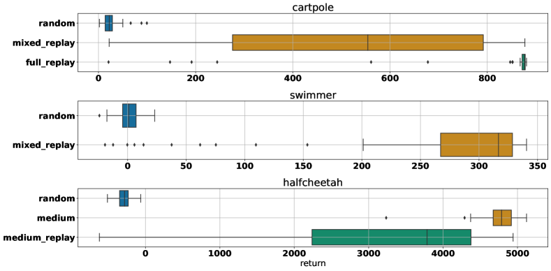
Figure 11: A comparison of the distribution of returns across the considered datasets.

A.3 Agent: SAC + planning

Soft Actor-Critic (SAC) (Haarnoja et al., 2018) is an off-policy algorithm that incorporates the maximum entropy framework, which encourages exploration by seeking to maximize the entropy of the policy in addition to the expected return. SAC uses a deep neural network to approximate the policy (actor) and the value functions (critics), employing two Q-value functions to mitigate positive bias in the policy improvement step typical of off-policy algorithms. This approach helps in learning more stable and effective policies for complex environments, making SAC particularly suitable for tasks with high-dimensional, continuous action spaces.

In addition to Dyna-style training of the SAC agent on the learned model with short rollouts a la MBPO (Janner et al., 2019), we use Model Predictive Control (MPC). MPC is the process of using the model recursively to plan and select the action sequence that maximizes the expected cumulative reward over a planning horizon $H$. The set of $K$ (population size) action sequences $\{(a^{k}_{t:t+H})_{k\in\{1,\dots,K\}}\}$ is usually generated by an evolutionary algorithm, e.g. Cross Entropy Method (CEM) (Chua et al., 2018). In this study, the pre-trained SAC guides the MPC process by generating candidate action sequences from the learned stochastic policy.

Appendix B Implementation details

For all the models, we use a neural network composed of a common number of hidden layers and two output heads (with Tanh activation functions) for the mean and standard deviation of the learned probabilistic dynamics (The standard deviation is fixed when we want to use the MSE loss). We use batch normalization (Ioffe & Szegedy, 2015), Dropout layers (Srivastava et al., 2014) ($p=10\%$), and set the learning rate of the Adam optimizer (Kingma & Ba, 2015) to $0.001$, the batch size to $64$, the number of common layers to $2$, and the number of hidden units to $256$ based on a hyperparameter search executed using the RAMP framework (Kégl et al., 2018). The evaluation metric of the hyperparameter optimization is the aggregated one-step validation R2 score across all the offline datasets. The neural networks are trained to predict the difference between the next state and the current state $\Delta_{t+1}=s_{t+1}-s_{t}$. More precisely, the baseline consists in the single-step model trained to predict the difference $\Delta_{t+1}$ using the one-step MSE. The other multi-step models, take their own predictions as input to predict the difference $\Delta_{t+h}=s_{t+h}-\hat{s}_{t+h-1}$ at horizon $h$

For the offline RL experiments, we use SAC agents from the StableBaselines3 open-source library (Raffin et al., 2021) while keeping its default hyperparameters. In the offline setting, we train the SAC agents for $500,000$ steps on a fixed model by generating short rollouts of length 100 from states of the the dataset selected uniformly at random. At evaluation time, the MPC planning is done by sampling $500$ action sequences from the SAC policy, and rolling out short rollouts of horizon $20$ for return computation. This return is then bootstrapped with the value function learned by SAC.

Appendix C Probabilistic interpretation

So far we have only considered deterministic models that directly learn to predict the next observation. However, it is very common in the literature to use probabilistic models that learn to predict the parameters of a dist ribution over the next observations (Chua et al., 2018; Janner et al., 2019; Nagabandi et al., 2018; Kégl et al., 2021), rather than a point estimate. Probabilistic models are useful because they enable uncertainty estimation, which can represent finite-sample fitting errors (epistemic uncertainty) and/or the intrinsic uncertainty in the environment dynamics (aleatory uncertainty).

In the probabilistic case, we represent $\hat{p}_{\theta}$ as a Gaussian over the next state

$$\hat{p}_{\theta}\big{(}s_{t+1}|s_{t},a_{t}\big{)}={\cal N}\big{(}s_{t+1}|\hat{\mu}_{\theta}(s_{t},a_{t}),\hat{\sigma}_{\theta}(s_{t},a_{t})\big{)},$$

where the parameters $(\hat{\mu}_{\theta},\hat{\sigma}_{\theta})$ are the output of the neural network. The loss function to train the probabilistic model on a transition$(s_{t},a_{t},s_{t+1})$ is the negative log-likelihood $L\big{(}s_{t+1},\hat{p}_{\theta}(\cdot|s_{t},a_{t})\big{)}=-\log\hat{p}_{\theta}(s_{t+1}|s_{t},a_{t})$.

Using this formulation, the $j^{th}$-horizon negative log-likelihood loss is

$$L\big{(}s_{t+j},\hat{p}_{\theta}^{j}(s_{t},{\bm{a}}_{t:t+j})\big{)} =-\log\hat{p}^{j}_{\theta}(s_{t+j}|s_{t},{\bm{a}}_{t:t+j})$$

$$=-\log{\cal N}\big{(}s_{t+j}|\hat{\mu}^{j}_{\theta}(s_{t},{\bm{a}}_{t:t+j}),\hat{\sigma}^{j}_{\theta}(s_{t},{\bm{a}}_{t:t+j})\big{)}.$$

Instead of the direct next prediction, the parameters of the distribution $\big{(}\hat{\mu}^{j}_{\theta}(s_{t},{\bm{a}}_{t:t+j}),\hat{\sigma}^{j}_{\theta}(s_{t},{\bm{a}}_{t:t+j})\big{)}$ represent the output of the model after $j$ recursive calls using the ground truth actions ${\bm{a}}_{t:t+j}$. From this definition, we can obtain the weighted multi-step MSE loss by solving a Maximum (joint) Likelihood Estimation (MLE) problem:

Proposition C.1.

(Multi-step MSE loss as MLE). Under the assumption of the conditional independence on $(s_{t},{\bm{a}}_{t:t+h})$, the weighted multi-step MSE loss can be recovered from the negative log-likelihood of the joint distribution of $(s_{t+1},\ldots,s_{t+h})={\bm{s}}_{t+1:t+h}$:

$$L\big{(}{\bm{s}}_{t+1:t+h},\hat{p}_{\theta}^{1:h}(s_{t},{\bm{a}}_{t:t+h})\big{)} =-\log\hat{p}^{1:h}_{\theta}({\bm{s}}_{t+1:t+h}|s_{t},{\bm{a}}_{t:t+h})$$

$$=-\log\Pi_{j=1}^{h}\hat{p}^{j}_{\theta}(s_{t+j}|s_{t},{\bm{a}}_{t:t+j})$$

$$=\underbrace{\sum_{j=1}^{h}\log\hat{\sigma}^{j}_{\theta}}_{\text{regularization}}+\underbrace{\sum_{j=1}^{h}\underbrace{\frac{1}{2(\hat{\sigma}^{j}_{\theta})^{2}}}_{\alpha_{j}}(s_{t+j}-\hat{\mu}^{j}_{\theta})^{2}}_{L_{\bm{\alpha}}}+\underbrace{C}_{constant}$$

with $\hat{\mu}^{j}_{\theta}=\hat{\mu}^{j}_{\theta}(s_{t},{\bm{a}}_{t:t+j})$ and $\hat{\sigma}^{j}_{\theta}=\hat{\sigma}^{j}_{\theta}(s_{t},{\bm{a}}_{t:t+j})$.

Remark C.2.

Proposition C.1 states the result in the case of uni-dimensional state spaces. While this is considered for simplicity, we can straight-forwardly generalize to the multi-variate case with the inverse of the covariance matrix as weight $\alpha_{j}=-\frac{1}{2}\hat{\Sigma}_{\theta}^{-1}$.

Can we automatically learn the weights using the MLE formulation in Proposition C.1?

To answer this question, we train a probabilistic model $\hat{p}_{\theta}$ to minimize the Negative Log-Likelihood (NLL) loss shown at Proposition C.1. When computing the multi-step loss at training time, the predicted states are obtained by sampling from the learned distribution using the reparametrization trick $\hat{s}_{t+j}=\hat{\mu}^{j}_{\theta}(s_{t},{\bm{a}}_{t:t+j})+\hat{\sigma}^{j}_{\theta}(s_{t},{\bm{a}}_{t:t+j})\cdot\xi$ where $\xi\sim{\cal N}(0,{\bm{I}})$. We refer to this as stoch-astic sampling, as opposed to det-erministic sampling that refers to MSE-based models where $\hat{s}_{t+j}=\hat{\mu}^{j}_{\theta}(s_{t},{\bm{a}}_{t:t+j})$.

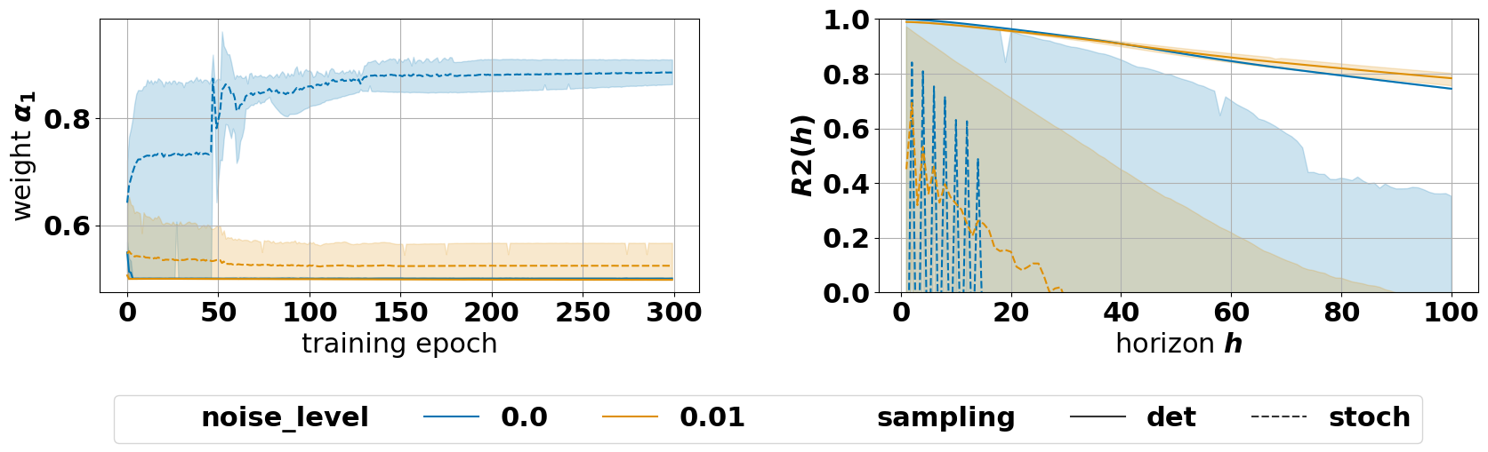
Figure 12: The left panel shows the normalized learned weights of a stochastic model trained using the $h=2$ multi-step loss. Basically, $\alpha_{1}=\frac{\frac{1}{|{\cal D}_{train}|}\sum_{{\cal D}_{train}}\frac{1}{2(\hat{\sigma}^{1}_{\theta})^{2}}}{\frac{1}{|{\cal D}_{train}|}\sum_{{\cal D}_{train}}\frac{1}{2(\hat{\sigma}^{1}_{\theta})^{2}}+\frac{1}{|{\cal D}_{train}|}\sum_{{\cal D}_{train}}\frac{1}{2\hat{(}{\sigma}^{2}_{\theta})^{2}}}$ and $\alpha_{2}=1-\alpha_{1}$. The right panel shows the $R2(h)$ curves on a held-out test dataset from the Cartpole swing-up random task.

Interestingly, we find that the stoch model automatically learns to put more weight on $h=1$ in absence of noise, while learning to balance the weights at $1\%$ noise (Figure 12). In the same dataset (Cartpole-Random with respectively $0\%$ and $1\%$ noise scale), we have found for the $h=2$ MSE-based model that the optimal weights were obtained by respectively $\beta=0.1$ ($\alpha_{1}=0.9$ and $\alpha_{2}=0.1$) and $\beta=2.0$ ($\alpha_{1}=0.33$ and $\alpha_{2}=0.66$). This result shows the potential of the MLE formulation to learn the correct weight profile depending on the intrinsic noise on the training data, which is captured through the learned variance.

In practice, the stoch model fails to predict accurately at future horizons (Figure 12), which is the reason why we don’t adopt this formulation in the main paper. We suspect that the model is underestimating the variance, leading to inaccurate predictions during inference and resulting in divergent trajectories. This issue stems from inadequate uncertainty propagation during the generation of rollouts from the stochastic model. In fact, accurate uncertainty quantification over future horizons necessitates the generation of multiple trajectories and the subsequent measurement of variance at the $j$-th horizon. We leave the exploration of this promising direction to future work.

Appendix D Additional experiments & results

D.1 Uni-dimensional linear system

D.1.1 Comparison with the data augmentation variant

To further understand the multi-step loss, we propose to reconduct the bias-variance analysis in Section 5.1 with a data augmentation variant that consists in training the $\alpha=1.0$ model (baseline) on an augmented dataset: ${\cal D}_{aug}=\{{\cal S}_{0},{\cal O}_{1}\}$, with the next states being $y=\{{\cal O}_{1},{\cal O}_{2}\}$.

Indeed, one may argue that the variance reduction gained by using the $\alpha=0.5$ multi-step loss is due to sampling the noise twice (both through ${\cal O}_{1}$, and ${\cal O}_{2}$), while the vanilla model only sees one realization of the noise through ${\cal O}_{1}$.

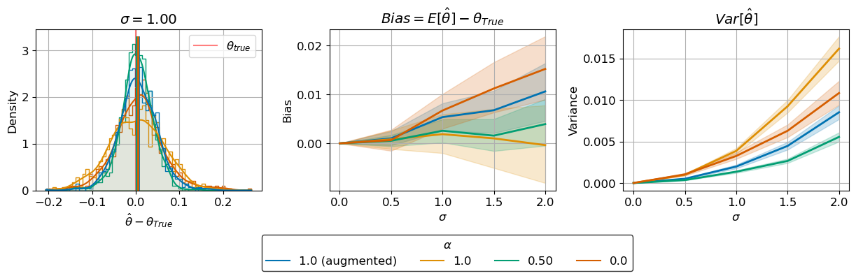
Figure 13: The left panel shows the density distribution of $\hat{\theta}-\theta_{true}$ for a fixed $\sigma$ of 1.0. The middle panel delineates the bias of the estimator, defined as $E[\hat{\theta}]-\theta_{true}$, across varying levels of $\sigma$, and weights $\alpha\in\{0,0.5,1\}$, in addition to the augmented variant of the $\alpha=1.0$ model. The right panel presents the variance of the estimator, $Var[\hat{\theta}]$, as a function of $\sigma$ for the same set of $\alpha$ values. The shaded regions represent the 95% bootstrap confidence intervals across 10 $\theta_{true}$ values, and 100 Monte-Carlo simulations.

As suggested by the previous reasoning, Figure 13 shows that indeed augmenting the training data of the baseline model reduces its variance, yet the multi-step model with $\alpha=0.5$ remains the optimal in terms of variance. Interestingly, we notice that the bias increases for the data-augmented model, this is due to the noise appearing in the inputs now, which changes the closed-form solutions derived in Section 5.1 and the estimator is no longer unbiased. We conclude on the optimality of the multi-step even in the data augmented case.

D.1.2 Analogy to noise reduction by averaging

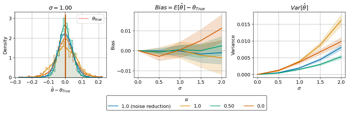
Figure 14: Similar to Figure 13, in addition to the noise reduction variant of the $\alpha=1.0$ model.

One way to increase the signal-to-noise ratio (SNR) is averaging (Ng & Goldberger, 2010; van Drongelen, 2007). It consists in sampling the same noisy event $k$ times, and observing a noise reduction in the average by a factor of $\sqrt{k}$. Although we have no guarantees about the factor of noise reduction observed when we use the multi-step loss, we hypothesize that the observed improvement is similar to that of noise reduction by averaging.

To test this hypothesis, we reconduct the bias-variance analysis in Section 5.1 and Section D.1.1 with a noise reduction variant that consists in training the $\alpha=1.0$ model (baseline) on a modified dataset: ${\cal D}_{reduc}=\{{\cal S}_{0}\}$, with the next states being $y=\{\frac{{\cal O}_{1}+{\cal O}^{\prime}_{1}}{2}\}$, where ${\cal O}_{1}$ and ${\cal O}^{\prime}_{1}$ are two realizations of the noisy next transitions. As illustrated in Figure 14, the noise reduction approach applied to the $h=1$ model demonstrated a significant reduction in variance while maintaining unbiasedness, a result that is supported by theoretical justification. Nonetheless, it is important to note that the multi-step model with $\alpha=0.5$ continues to display a lower variance, albeit with a marginally increased bias.

D.2 Two-parameter Non-linear system

D.2.1 The loss landscape and approximate global minima

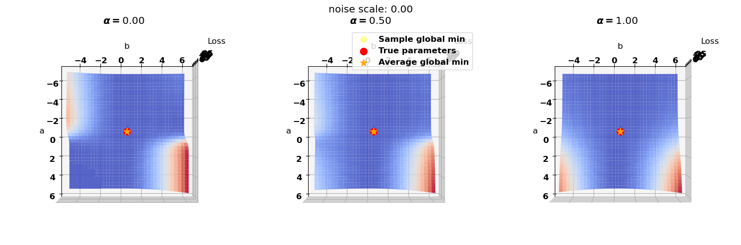
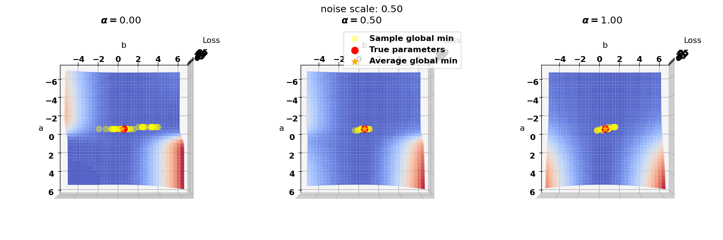
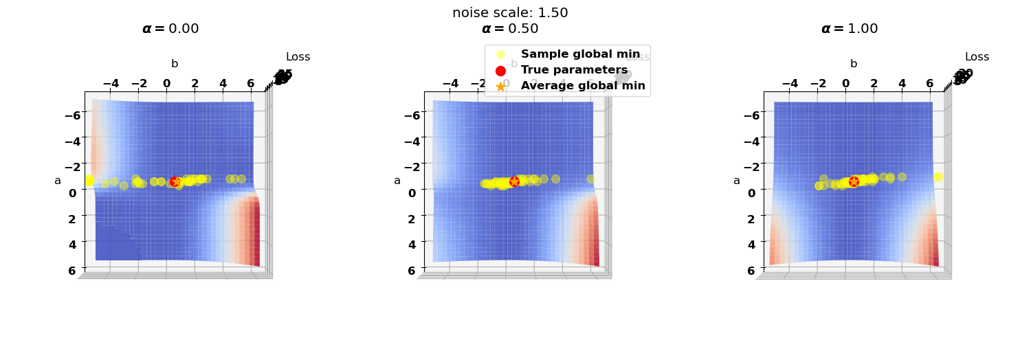
Figure 15: This figure illustrates the impact of noise on the optimization of a multi-step MSE loss function by displaying loss landscapes at varying noise levels and alpha ($\alpha$) values. The true parameters ($\theta^{true}$) are marked with red dots. Each row represents a different level of noise, with yellow dots indicating individual instances of global minima and orange stars denoting their average.

In the non-linear case, the problem of computing the minimizers of the loss function is intractable. To build an understanding about the optimization challenges in this setup, we tried to replicate the same analysis we did in the linear case, visualizing the loss landscape and its approximate global minima Figure 15.

The global minima in Figure 15 were determined by evaluating the loss function across a finely meshed grid surrounding the true parameters $\theta^{true}$. This process was carried out for ten distinct sets of future observations at varying noise levels. The resulting data include the average loss surface, individual instances of global minima (indicated by yellow dots) and their mean (shown as an orange star). In absence of noise, all global minima are aligned with $\theta^{true}$, serving as a preliminary validation of the multi-step loss’s consistency. However, as the noise level increases, the challenge of optimizing the two-step MSE loss becomes more and more apparent, evidenced by an increasing number of minimum points diverging from the true parameters. In contrast, the model with an intermediate value of $\alpha=0.5$ either matched or outperformed the baseline model ($\alpha=1$) in terms of the proximity of the global minima to the true parameters. Consequently, in this basic non-linear scenario, it is evident that the multi-step loss does not introduce significant optimization difficulties at lower $\alpha$ values.

D.2.2 Details of the experiment in Section 5.2

The goal of the experiment in Section 5.2 is to assess the solutions of the multi-step MSE loss after training. Indeed, the intractability of the optimization problem forces to only analyze the solution after a gradient-based optimization procedure, all while integrating counfounding factors of this latter. The confounding factors that influence the outcome of the optimization incude: the optimizer, the initial points distribution, the learning rate, among others.

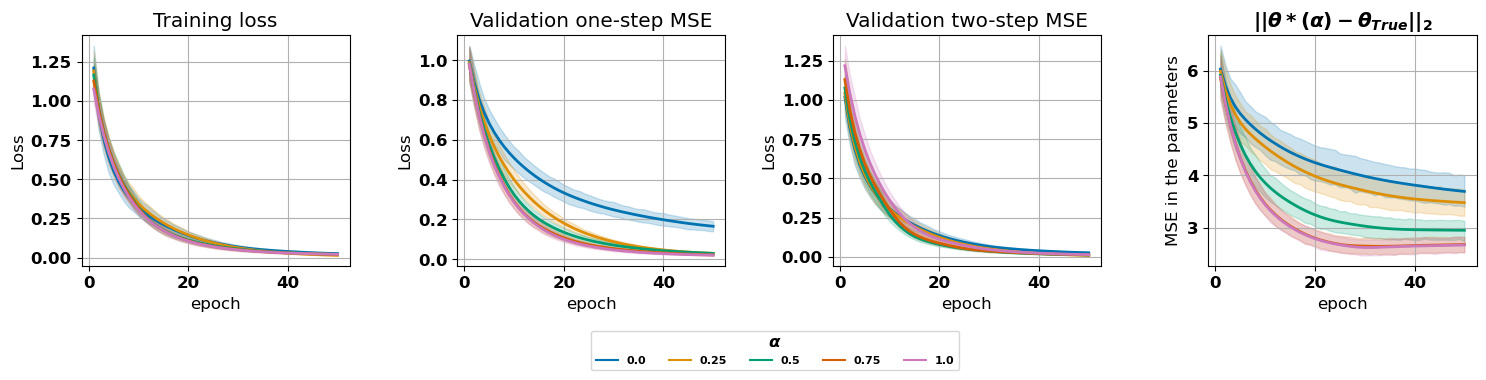
Figure 16: The three left panels show the training, the one-step, and the two-step validation losses across 50 training epochs. The right panel show the evolution of the distance of the NN parameters to the system parameters during training.

In this study we generate $10$ Monte-Carlo simulations for each of: $10$ randomly sampled initial points, $3$ initialization distributions (default, uniform, Xavier_uniform), $2$ optimizers (Adam, SGD), $3$ noise levels ($0\%$, $20\%$, and $40\%$), 5 different values of the multi-step loss parameter $\alpha\in\{0,0.25,0.5,0.75,1\}$. For each of these experiments, we train the neural network to minimize the multi-step MSE loss $L_{\alpha}$ for $60$ epochs. We report and analyze the validation losses and proximity to the true parameters in Figure 5, Section 5.2.

Figure 16 shows the per-epoch training and validation loss curves, in addition to the MSE between the model parameters and the true parameters.

D.3 Static evaluation

D.3.1 $\overline{R2}(100)$ table

The static evaluation has been conducted by training models on the multi-step loss for different values of $h\in\{2,3,4,10\}$ and $\beta\in\{0.1,0.3,0.5,0.75,1.0,1.5,2.0,3.0,5.0,20.0\}$. Table 4 shows the corresponding test $\overline{R2}(100)$ scores and their standard deviations after the symbol $\pm$. For each horizon $h$, we show the best value of the $\beta$ parameter, as it’s different across environments, datasets, and noise scales.

Environment	Dataset	Noise scale	One-step	Multi-step
				h=2 $[\beta]$	h=3 $[\beta]$	h=4 $[\beta]$	h=10 $[\beta]$
Cartpole swing-up	random	0	972 +- 4	975 +- 1 [0.1]	977 +- 2 [0.3]	980 +- 1 [0.1]	986 +- 1 [0.75]
		0.01	864 +- 5	930 +- 1 [2.0]	950 +- 2 [2.0]	946 +- 3 [1.0]	954 +- 4 [0.75]
		0.02	508 +- 16	690 +- 15 [2.0]	769 +- 7 [2.0]	812 +- 7 [1.5]	836 +- 7 [0.75]
	mixed_replay	0	812 +- 106	915 +- 22 [0.75]	921 +- 32 [2.0]	925 +- 24 [0.5]	931 +- 20 [0.75]
		0.01	541 +- 51	574 +- 26 [0.1]	659 +- 44 [3.0]	653 +- 51 [1.5]	679 +- 38 [0.75]
		0.02	428 +- 9	335 +- 4 [2.0]	459 +- 71 [0.75]	481 +- 12 [1.0]	457 +- 38 [0.75]
	full_replay	0	705 +- 52	828 +- 6 [2.0]	843 +- 42 [2.0]	858 +- 32 [0.75]	880 +- 21 [0.5]
		0.01	714 +- 7	709 +- 10 [0.1]	718 +- 6 [1.5]	722 +- 33 [0.75]	683 +- 32 [0.1]
		0.02	530 +- 14	551 +- 34 [0.1]	527 +- 21 [1.5]	530 +- 46 [0.1]	541 +- 24 [0.1]
Swimmer	random	0	983 +- 1	974 +- 3 [0.1]	978 +- 0 [0.1]	975 +- 1 [0.1]	974 +- 2 [0.1]
		0.01	934 +- 6	941 +- 0 [0.1]	941 +- 2 [0.1]	942 +- 1 [0.5]	943 +- 2 [0.5]
		0.02	865 +- 14	869 +- 17 [0.1]	880 +- 8 [0.5]	892 +- 4 [0.5]	891 +- 4 [0.5]
	mixed_replay	0	609 +- 46	680 +- 184 [20.0]	734 +- 18 [20.0]	875 +- 25 [3.0]	735 +- 120 [0.75]
		0.01	874 +- 14	904 +- 16 [0.5]	901 +- 16 [3.0]	936 +- 5 [0.1]	920 +- 8 [0.75]
		0.02	850 +- 13	893 +- 8 [1.0]	878 +- 6 [0.3]	886 +- 4 [1.0]	883 +- 8 [0.75]
Halfcheetah	random	0	755 +- 3	746 +- 7 [0.1]	775 +- 3 [0.1]	765 +- 9 [0.5]	766 +- 5 [0.3]
		0.01	737 +- 4	732 +- 27 [0.1]	756 +- 9 [0.1]	763 +- 6 [0.1]	725 +- 5 [0.5]
		0.02	704 +- 3	711 +- 17 [0.1]	709 +- 23 [0.1]	701 +- 3 [0.5]	731 +- 0 [0.3]
	medium	0	516 +- 19	268 +- 51 [0.1]	547 +- 10 [0.3]	562 +- 63 [0.3]	640 +- 13 [0.3]
		0.01	691 +- 11	634 +- 20 [0.1]	674 +- 28 [0.1]	695 +- 3 [0.1]	710 +- 4 [0.1]
		0.02	718 +- 4	422 +- 242 [0.1]	675 +- 15 [0.1]	690 +- 1 [0.1]	702 +- 13 [0.1]
	medium_replay	0	541 +- 54	446 +- 70 [3.0]	589 +- 15 [0.75]	632 +- 7 [0.75]	771 +- 12 [0.5]
		0.01	709 +- 12	725 +- 4 [0.1]	737 +- 7 [0.1]	737 +- 16 [0.1]	773 +- 9 [0.3]
		0.02	687 +- 26	723 +- 16 [0.1]	731 +- 6 [0.1]	765 +- 18 [0.3]	750 +- 7 [0.3]

Table 4: $\overline{R2}(100)$ for different environments, datasets, and noise scales. We highlight entries that have significantly larger score. In addition, to the mean ${}^{p}m$ standard deviation of the reported metric, the table also shows the best $\beta$ selected for each loss horizon $h$.

D.3.2 The weight profile and the effective horizon

We can define the effective horizon $h_{e}$ that reflects the prediction horizon at which we effectively optimize the prediction error: given a weighted multi-step loss $L_{\bm{\alpha}}$ with nominal horizon $h$ and weights ${\bm{\alpha}}$, the effective horizon $h_{e}$ is defined as $h_{e}=\sum_{i=1}^{h}\alpha_{i}\cdot i$.

For a given model trained using the multi-step loss, the optimal effective horizon is an indication of the time scale needed for optimal performance. However, models that have a different nominal horizon $h$ and the same effective horizon $h_{e}$ do not necessarily have the same performance. Precisely, the loss with the larger nominal horizon is setting small weights on the furthest horizons, which has a direct impact on the loss landscape and consequently on the optimization process.

Table 5 shows the optimal effective horizon $h_{e}$, and the exponentially parametrized weight profiles (characterized by the decay parameter $\beta$), for different values of the horizon $h$ and the noise scale $\sigma$.

Table 5: Best $h_{e}(\beta)$ values found with a grid search for each horizon and each noise scale. The values are averaged over the eight datasets.

	horizon $h$
	2	3	4	10
$\sigma$ (%)	$h_{e}\hskip 2.84544pt(\beta)$
0.0	1.30 (0.81)	1.48 (0.45)	1.58 (0.41)	2.09 (0.46)
0.01	1.26 (0.56)	1.65 (0.76)	1.74 (0.51)	2.23 (0.47)
0.02	1.36 (0.86)	1.65 (0.72)	2.08 (0.78)	2.72 (0.54)
0.03	1.33 (0.67)	1.95 (1.21)	2.13 (0.81)	2.33 (0.50)
0.04	1.40 (0.74)	1.88 (1.01)	2.02 (0.74)	2.49 (0.55)
0.05	1.49 (1.33)	1.76 (0.83)	2.28 (0.97)	2.22 (0.51)

The main insight of Table 5 is that regardless of the nominal horizon $h$, the effective horizon $h_{e}$ (and equivalently the decay parameter $\beta$) increases with the noise scale. This finding supports the idea that multi-step models are increasingly needed when incorporating information from the future is crucial to achieve noise reduction. As discussed in the previous experiment, the results are highly dependent on the task (environment/dataset), while in Table 5 we aggregate the results across tasks, and still observe the increasing trend.

Another important result highlighted in Table 5 is the upper bound on the effective horizon ($h_{e}$ does not go beyond $2.52$), even when the nominal horizon is large (e.g 10). This suggests that while putting weight on future horizons error does help the model, it is not beneficial to fully optimize for these horizons. Indeed, the additional components of the multi-step MSE loss act as a regularizer to the one-step loss, rather than a completely different training objective.

D.3.3 $R2(h)$ curves

In this section, we show the full $R2(h)$ curves for all environments / datasets.

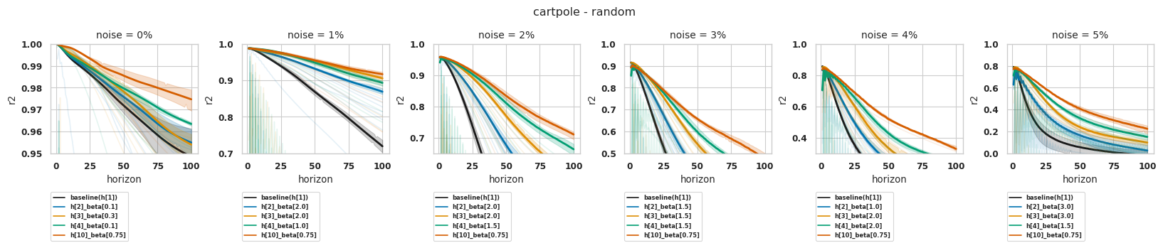
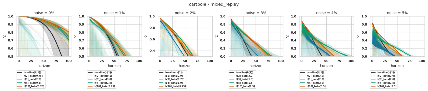
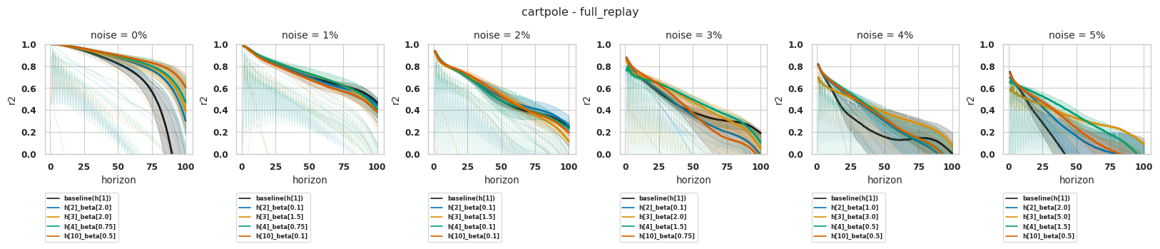
Figure 17: Cartpole.

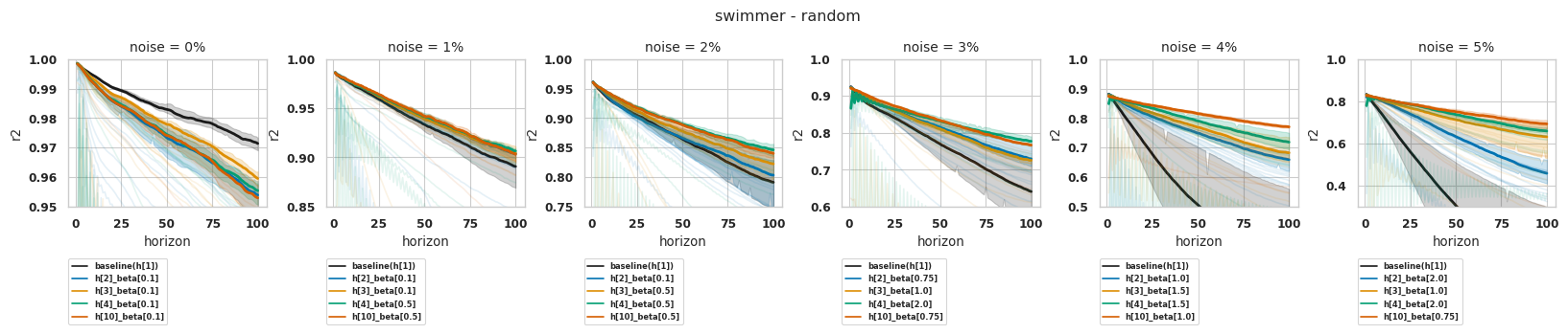
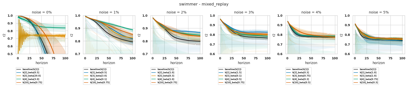
Figure 18: Swimmer.

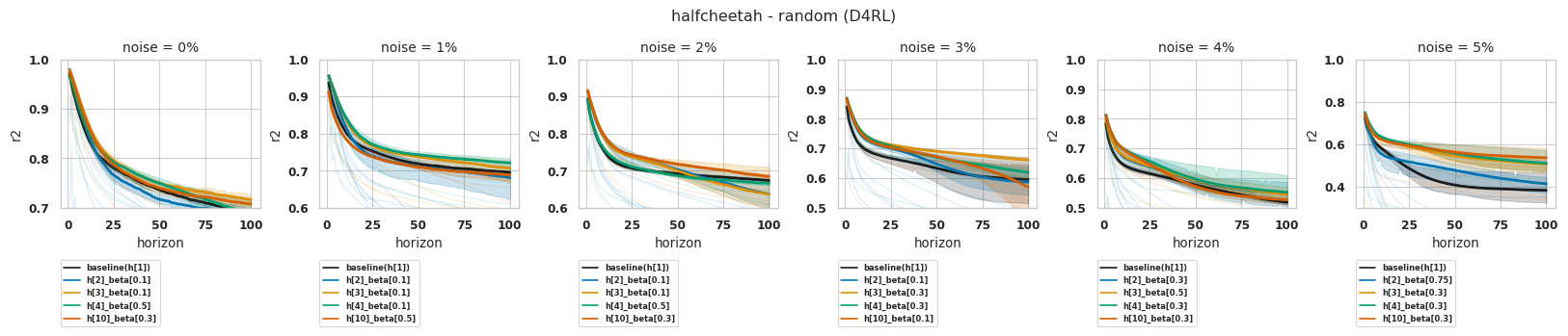
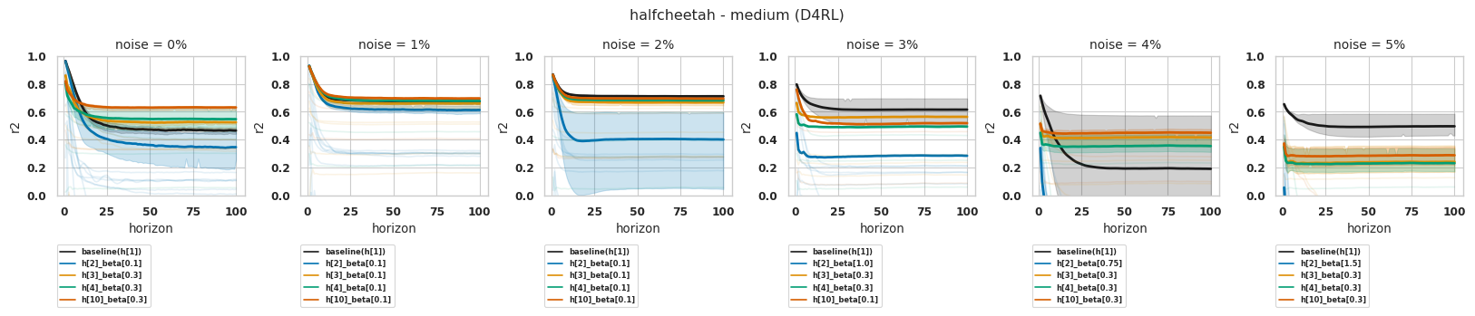
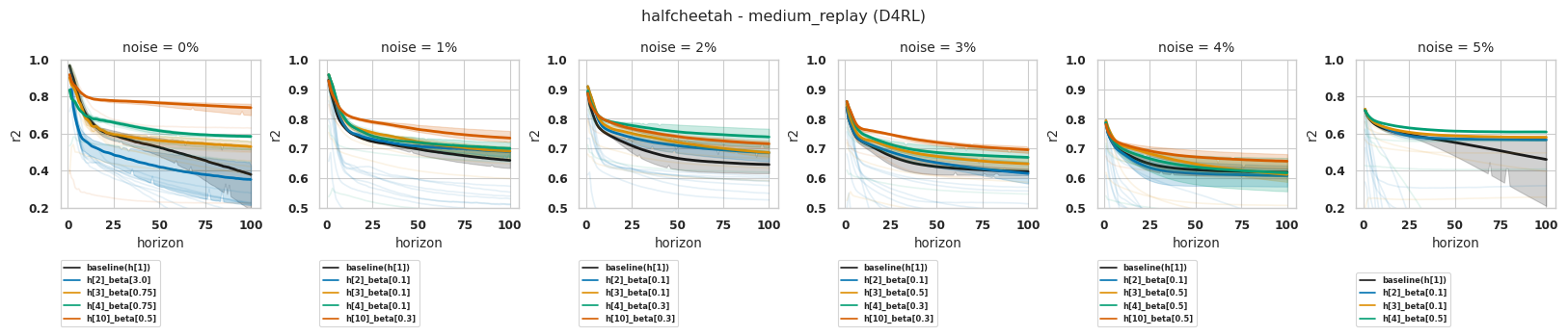
Figure 19: Halfcheetah.

References

- Noa (2023) DMBP: Diffusion model based predictor for robust offline reinforcement learning against state observation perturbations. October 2023. URL https://openreview.net/forum?id=ZULjcYLWKe.
- Abbeel et al. (2005) Abbeel, P., Ganapathi, V., and Ng, A. Learning vehicular dynamics, with application to modeling helicopters. Advances in Neural Information Processing Systems, 18, 2005. URL https://proceedings.neurips.cc/paper/2005/hash/09b69adcd7cbae914c6204984097d2da-Abstract.html. Read.
- Ben Taieb & Bontempi (2012) Ben Taieb, S. and Bontempi, G. Recursive Multi-step Time Series Forecasting by Perturbing Data, January 2012. URL https://ieeexplore.ieee.org/abstract/document/6137274.
- Ben Taieb et al. (2012) Ben Taieb, S., Bontempi, G., Atiya, A. F., and Sorjamaa, A. A review and comparison of strategies for multi-step ahead time series forecasting based on the NN5 forecasting competition. Expert Systems with Applications, 39(8):7067–7083, June 2012. ISSN 0957-4174. doi: 10.1016/j.eswa.2012.01.039. URL https://www.sciencedirect.com/science/article/pii/S0957417412000528.
- Bengio et al. (2015) Bengio, S., Vinyals, O., Jaitly, N., and Shazeer, N. Scheduled Sampling for Sequence Prediction with Recurrent Neural Networks, September 2015. URL http://arxiv.org/abs/1506.03099.
- Brockman et al. (2016) Brockman, G., Cheung, V., Pettersson, L., Schneider, J., Schulman, J., Tang, J., and Zaremba, W. OpenAI gym, 2016.
- Byravan et al. (2021) Byravan, A., Hasenclever, L., Trochim, P., Mirza, M., Ialongo, A. D., Tassa, Y., Springenberg, J. T., Abdolmaleki, A., Heess, N., Merel, J., and Riedmiller, M. A. Evaluating model-based planning and planner amortization for continuous control. CoRR, abs/2110.03363, 2021. URL https://arxiv.org/abs/2110.03363.
- Chandra et al. (2021) Chandra, R., Goyal, S., and Gupta, R. Evaluation of deep learning models for multi-step ahead time series prediction. IEEE Access, 9:83105–83123, 2021. ISSN 2169-3536. doi: 10.1109/ACCESS.2021.3085085. URL http://arxiv.org/abs/2103.14250. arXiv:2103.14250 [cs].
- Chua et al. (2018) Chua, K., Calandra, R., McAllister, R., and Levine, S. Deep reinforcement learning in a handful of trials using probabilistic dynamics models. In Advances in Neural Information Processing Systems 31, pp. 4754–4765. Curran Associates, Inc., 2018.
- Fraedrich & Rückert (1998) Fraedrich, K. and Rückert, B. Metric adaption for analog forecasting. Physica A: Statistical Mechanics and its Applications, 253(1):379–393, 1998. ISSN 0378-4371. doi: https://doi.org/10.1016/S0378-4371(97)00668-7. URL https://www.sciencedirect.com/science/article/pii/S0378437197006687.
- Haarnoja et al. (2018) Haarnoja, T., Zhou, A., Abbeel, P., and Levine, S. Soft Actor-Critic: Off-Policy Maximum Entropy Deep Reinforcement Learning with a Stochastic Actor. In Dy, J. and Krause, A. (eds.), Proceedings of the 35th International Conference on Machine Learning, volume 80 of Proceedings of Machine Learning Research, pp. 1861–1870. PMLR, 10–15 Jul 2018.
- Hess et al. (2023) Hess, F., Monfared, Z., Brenner, M., and Durstewitz, D. Generalized Teacher Forcing for Learning Chaotic Dynamics, October 2023. URL http://arxiv.org/abs/2306.04406. arXiv:2306.04406 [nlin].
- Huszár (2015) Huszár, F. How (not) to Train your Generative Model: Scheduled Sampling, Likelihood, Adversary?, November 2015. URL http://arxiv.org/abs/1511.05101.
- Ioffe & Szegedy (2015) Ioffe, S. and Szegedy, C. Batch normalization: Accelerating deep network training by reducing internal covariate shift. In Proceedings of the 32nd International Conference on International Conference on Machine Learning - Volume 37, ICML’15, pp. 448–456. JMLR.org, 2015.
- Janner et al. (2019) Janner, M., Fu, J., Zhang, M., and Levine, S. When to trust your model: Model-based policy optimization. In Wallach, H., Larochelle, H., Beygelzimer, A., d'Alché-Buc, F., Fox, E., and Garnett, R. (eds.), Advances in Neural Information Processing Systems, volume 32. Curran Associates, Inc., 2019.
- Kégl et al. (2018) Kégl, B., Boucaud, A., Cherti, M., Kazakci, A., Gramfort, A., Lemaitre, G., den Bossche, J. V., Benbouzid, D., and Marini, C. The RAMP framework: from reproducibility to transparency in the design and optimization of scientific workflows. In ICML workshop on Reproducibility in Machine Learning, 2018.
- Kégl et al. (2021) Kégl, B., Hurtado, G., and Thomas, A. Model-based micro-data reinforcement learning: what are the crucial model properties and which model to choose? In International Conference on Learning Representations, 2021. URL https://openreview.net/forum?id=p5uylG94S68.
- Kingma & Ba (2015) Kingma, D. P. and Ba, J. Adam: A method for stochastic optimization. In Bengio, Y. and LeCun, Y. (eds.), 3rd International Conference on Learning Representations, ICLR 2015, San Diego, CA, USA, May 7-9, 2015, Conference Track Proceedings, 2015. URL http://arxiv.org/abs/1412.6980.
- Lamb et al. (2016) Lamb, A. M., ALIAS PARTH GOYAL, A. G., Zhang, Y., Zhang, S., Courville, A. C., and Bengio, Y. Professor Forcing: A New Algorithm for Training Recurrent Networks. In Advances in Neural Information Processing Systems, volume 29. Curran Associates, Inc., 2016. URL https://proceedings.neurips.cc/paper_files/paper/2016/hash/16026d60ff9b54410b3435b403afd226-Abstract.html.
- Lambert et al. (2021) Lambert, N., Amos, B., Yadan, O., and Calandra, R. Objective mismatch in model-based reinforcement learning, 2021.
- Lambert et al. (2022) Lambert, N., Pister, K., and Calandra, R. Investigating Compounding Prediction Errors in Learned Dynamics Models, March 2022. URL http://arxiv.org/abs/2203.09637. arXiv:2203.09637 [cs].
- Levine et al. (2020) Levine, S., Kumar, A., Tucker, G., and Fu, J. Offline reinforcement learning: Tutorial, review, and perspectives on open problems. arXiv preprint arXiv:2005.01643, 2020.
- Lutter et al. (2021) Lutter, M., Hasenclever, L., Byravan, A., Dulac-Arnold, G., Trochim, P., Heess, N., Merel, J., and Tassa, Y. Learning Dynamics Models for Model Predictive Agents, September 2021. URL http://arxiv.org/abs/2109.14311.
- McNames (2002) McNames, J. Local averaging optimization for chaotic time series prediction. Neurocomputing, 48(1):279–297, 2002. ISSN 0925-2312. doi: https://doi.org/10.1016/S0925-2312(01)00647-6. URL https://www.sciencedirect.com/science/article/pii/S0925231201006476.
- Mnih et al. (2015) Mnih, V., Kavukcuoglu, K., Silver, D., Rusu, A. A., Veness, J., Bellemare, M. G., Graves, A., Riedmiller, M., Fidjeland, A. K., Ostrovski, G., Petersen, S., Beattie, C., Sadik, A., Antonoglou, I., King, H., Kumaran, D., Wierstra, D., Legg, S., and Hassabis, D. Human-level control through deep reinforcement learning. Nature, 518(7540):529–533, 2015.
- Nagabandi et al. (2018) Nagabandi, A., Kahn, G., Fearing, R. S., and Levine, S. Neural network dynamics for model-based deep reinforcement learning with model-free fine-tuning. In 2018 IEEE International Conference on Robotics and Automation, ICRA 2018, pp. 7559–7566. IEEE, 2018.
- Ng & Goldberger (2010) Ng, J. and Goldberger, J. J. Signal Averaging for Noise Reduction, pp. 69–77. Springer London, London, 2010. ISBN 978-1-84882-515-4. doi: 10.1007/978-1-84882-515-4˙7. URL https://doi.org/10.1007/978-1-84882-515-4_7.
- Pattanaik et al. (2017) Pattanaik, A., Tang, Z., Liu, S., Bommannan, G., and Chowdhary, G. Robust Deep Reinforcement Learning with Adversarial Attacks, December 2017. URL http://arxiv.org/abs/1712.03632. arXiv:1712.03632 [cs].
- Pineda (1988) Pineda, F. J. Dynamics and architecture for neural computation. Journal of Complexity, 4(3):216–245, September 1988. ISSN 0885-064X. doi: 10.1016/0885-064X(88)90021-0. URL https://www.sciencedirect.com/science/article/pii/0885064X88900210.
- Precup & Sutton (1997) Precup, D. and Sutton, R. S. Multi-time Models for Temporally Abstract Planning. In Advances in Neural Information Processing Systems, volume 10. MIT Press, 1997. URL https://proceedings.neurips.cc/paper_files/paper/1997/hash/a9be4c2a4041cadbf9d61ae16dd1389e-Abstract.html.
- Precup et al. (1998) Precup, D., Sutton, R. S., and Singh, S. Theoretical results on reinforcement learning with temporally abstract options. In Nédellec, C. and Rouveirol, C. (eds.), Machine Learning: ECML-98, Lecture Notes in Computer Science, pp. 382–393, Berlin, Heidelberg, 1998. Springer. ISBN 978-3-540-69781-7. doi: 10.1007/BFb0026709.
- Raffin et al. (2021) Raffin, A., Hill, A., Gleave, A., Kanervisto, A., Ernestus, M., and Dormann, N. Stable-baselines3: Reliable reinforcement learning implementations. Journal of Machine Learning Research, 22(268):1–8, 2021. URL http://jmlr.org/papers/v22/20-1364.html.
- Silver et al. (2017) Silver, D., Hubert, T., Schrittwieser, J., Antonoglou, I., Lai, M., Guez, A., Lanctot, M., Sifre, L., Kumaran, D., Graepel, T., Lillicrap, T., Simonyan, K., and Hassabis, D. Mastering chess and shogi by self-play with a general reinforcement learning algorithm, 2017.
- Silver et al. (2018) Silver, D., Hubert, T., Schrittwieser, J., Antonoglou, I., Lai, M., Guez, A., Lanctot, M., Sifre, L., Kumaran, D., Graepel, T., Lillicrap, T., Simonyan, K., and Hassabis, D. A general reinforcement learning algorithm that masters Chess, Shogi, and Go through self-play. Science, 362(6419):1140–1144, 2018. ISSN 0036-8075. doi: 10.1126/science.aar6404.
- Singh (1992) Singh, S. P. Scaling Reinforcement Learning Algorithms by Learning Variable Temporal Resolution Models. In Sleeman, D. and Edwards, P. (eds.), Machine Learning Proceedings 1992, pp. 406–415. Morgan Kaufmann, San Francisco (CA), January 1992. ISBN 978-1-55860-247-2. doi: 10.1016/B978-1-55860-247-2.50058-9. URL https://www.sciencedirect.com/science/article/pii/B9781558602472500589.
- Srivastava et al. (2014) Srivastava, N., Hinton, G., Krizhevsky, A., Sutskever, I., and Salakhutdinov, R. Dropout: A simple way to prevent neural networks from overfitting. Journal of Machine Learning Research, 15(56):1929–1958, 2014. URL http://jmlr.org/papers/v15/srivastava14a.html.
- Sun et al. (2023) Sun, K., Zhao, Y., Jui, S., and Kong, L. Exploring the Training Robustness of Distributional Reinforcement Learning against Noisy State Observations, June 2023. URL http://arxiv.org/abs/2109.08776. arXiv:2109.08776 [cs].
- Sutton (1995) Sutton, R. S. TD Models: Modeling the World at a Mixture of Time Scales. In Prieditis, A. and Russell, S. (eds.), Machine Learning Proceedings 1995, pp. 531–539. Morgan Kaufmann, San Francisco (CA), January 1995. ISBN 978-1-55860-377-6. doi: 10.1016/B978-1-55860-377-6.50072-4. URL https://www.sciencedirect.com/science/article/pii/B9781558603776500724.
- Sutton & Pinette (1985) Sutton, R. S. and Pinette, B. The learning of world models by connectionist networks, 1985.
- Sutton et al. (1999) Sutton, R. S., Precup, D., and Singh, S. Between MDPs and semi-MDPs: A framework for temporal abstraction in reinforcement learning. Artificial Intelligence, 112(1):181–211, August 1999. ISSN 0004-3702. doi: 10.1016/S0004-3702(99)00052-1. URL https://www.sciencedirect.com/science/article/pii/S0004370299000521.
- Talvitie (2014) Talvitie, E. Model Regularization for Stable Sample Rollouts. 2014.
- Talvitie (2017) Talvitie, E. Self-Correcting Models for Model-Based Reinforcement Learning. Proceedings of the AAAI Conference on Artificial Intelligence, 31(1), February 2017. ISSN 2374-3468, 2159-5399. doi: 10.1609/aaai.v31i1.10850. URL https://ojs.aaai.org/index.php/AAAI/article/view/10850.
- Tanaka et al. (1995) Tanaka, N., Okamoto, H., and Naito, M. N. M. An optimal metric for predicting chaotic time series. Japanese Journal of Applied Physics, 34(1R):388, jan 1995. doi: 10.1143/JJAP.34.388. URL https://dx.doi.org/10.1143/JJAP.34.388.
- Tassa et al. (2018) Tassa, Y., Doron, Y., Muldal, A., Erez, T., Li, Y., de Las Casas, D., Budden, D., Abdolmaleki, A., Merel, J., Lefrancq, A., Lillicrap, T. P., and Riedmiller, M. A. Deepmind control suite. CoRR, abs/1801.00690, 2018. URL http://arxiv.org/abs/1801.00690.
- Todorov et al. (2012) Todorov, E., Erez, T., and Tassa, Y. Mujoco: A physics engine for model-based control. In 2012 IEEE/RSJ International Conference on Intelligent Robots and Systems, pp. 5026–5033, 2012. doi: 10.1109/IROS.2012.6386109.
- van Drongelen (2007) van Drongelen, W. 4 - signal averaging. In van Drongelen, W. (ed.), Signal Processing for Neuroscientists, pp. 55–70. Academic Press, Burlington, 2007. ISBN 978-0-12-370867-0. doi: https://doi.org/10.1016/B978-012370867-0/50004-8. URL https://www.sciencedirect.com/science/article/pii/B9780123708670500048.
- Venkatraman et al. (2015) Venkatraman, A., Hebert, M., and Bagnell, J. Improving Multi-Step Prediction of Learned Time Series Models. Proceedings of the AAAI Conference on Artificial Intelligence, 29(1), February 2015. ISSN 2374-3468, 2159-5399. doi: 10.1609/aaai.v29i1.9590. URL https://ojs.aaai.org/index.php/AAAI/article/view/9590.
- Vinyals et al. (2019) Vinyals, O., Babuschkin, I., Czarnecki, W. M., Mathieu, M., Dudzik, A., Chung, J., Choi, D. H., Powell, R., Ewalds, T., Georgiev, P., Oh, J., Horgan, D., Kroiss, M., Danihelka, I., Huang, A., Sifre, L., Cai, T., Agapiou, J. P., Jaderberg, M., Vezhnevets, A. S., Leblond, R., Pohlen, T., Dalibard, V., Budden, D., Sulsky, Y., Molloy, J., Paine, T. L., Gulcehre, C., Wang, Z., Pfaff, T., Wu, Y., Ring, R., Yogatama, D., Wünsch, D., McKinney, K., Smith, O., Schaul, T., Lillicrap, T. P., Kavukcuoglu, K., Hassabis, D., Apps, C., and Silver, D. Grandmaster level in starcraft ii using multi-agent reinforcement learning. Nature, pp. 1–5, 2019.
- Williams & Zipser (1989) Williams, R. J. and Zipser, D. A Learning Algorithm for Continually Running Fully Recurrent Neural Networks. Neural Computation, 1(2):270–280, June 1989. ISSN 0899-7667. doi: 10.1162/neco.1989.1.2.270. URL https://ieeexplore.ieee.org/document/6795228. Conference Name: Neural Computation.
- Xu et al. (2018) Xu, H., Li, Y., Tian, Y., Darrell, T., and Ma, T. Algorithmic framework for model-based reinforcement learning with theoretical guarantees. CoRR, abs/1807.03858, 2018. URL http://arxiv.org/abs/1807.03858.
- Yu et al. (2020) Yu, T., Thomas, G., Yu, L., Ermon, S., Zou, J. Y., Levine, S., Finn, C., and Ma, T. Mopo: Model-based offline policy optimization. In Larochelle, H., Ranzato, M., Hadsell, R., Balcan, M., and Lin, H. (eds.), Advances in Neural Information Processing Systems, volume 33, pp. 14129–14142. Curran Associates, Inc., 2020. URL https://proceedings.neurips.cc/paper/2020/file/a322852ce0df73e204b7e67cbbef0d0a-Paper.pdf.
- Zhang et al. (2021) Zhang, H., Chen, H., Xiao, C., Li, B., Liu, M., Boning, D., and Hsieh, C.-J. Robust Deep Reinforcement Learning against Adversarial Perturbations on State Observations, July 2021. URL http://arxiv.org/abs/2003.08938. arXiv:2003.08938 [cs, stat].