Enhancing Neural Subset Selection: Integrating Background Information into Set Representations

Abstract

Learning neural subset selection tasks, such as compound selection in AI-aided drug discovery, have become increasingly pivotal across diverse applications. The existing methodologies in the field primarily concentrate on constructing models that capture the relationship between utility function values and subsets within their respective supersets. However, these approaches tend to overlook the valuable information contained within the superset when utilizing neural networks to model set functions. In this work, we address this oversight by adopting a probabilistic perspective. Our theoretical findings demonstrate that when the target value is conditioned on both the input set and subset, it is essential to incorporate an invariant sufficient statistic of the superset into the subset of interest for effective learning. This ensures that the output value remains invariant to permutations of the subset and its corresponding superset, enabling identification of the specific superset from which the subset originated. Motivated by these insights, we propose a simple yet effective information aggregation module designed to merge the representations of subsets and supersets from a permutation invariance perspective. Comprehensive empirical evaluations across diverse tasks and datasets validate the enhanced efficacy of our approach over conventional methods, underscoring the practicality and potency of our proposed strategies in real-world contexts.

1 Introduction

The prediction of set-valued outputs plays a crucial role in various real-world applications. For instance, anomaly detection involves identifying outliers from a majority of data (Zhang et al., 2020), and compound selection in drug discovery aims to extract the most effective compounds from a given compound database (Gimeno et al., 2019). In these applications, there exists an implicit learning of a set function (Rezatofighi et al., 2017; Zaheer et al., 2017) that quantifies the utility of a given set input, where the highest utility value corresponds to the most desirable set output.

More formally, let’s consider the compound selection task: given a compound database $V$, the goal is to select a subset of compounds $S^{*}\subseteq V$ that exhibit the highest utility. This utility can be modeled by a parameterized utility function $F_{\theta}(S;V)$, and the optimization criteria can be expressed as:

$$S^{*}=\operatorname*{arg\,max}_{S\in 2^{V}}F_{\theta}(S;V).$$ (1)

One straightforward method is to explicitly model the utility by learning $U=F_{\theta}(S;V)$ using supervised data in the form of $\{(S_{i},V_{i}),U_{i}\}_{i=1}^{N},$ where $U_{i}$ represents the true utility value of subset $S_{i}$ given $V_{i}$. However, this training approach becomes prohibitively expensive due to the need for constructing a large amount of supervision signals (Balcan & Harvey, 2018).

To address this limitation, another way is to solve Eq.1 with an implicit learning approach from a probabilistic perspective. Specifically, it is required to utilize data in the form of $\{(V_{i},S_{i}^{*})\}_{i=1}^{N}$, where $S_{i}^{*}$ represents the optimal subset corresponding to $V_{i}$. The goal is to estimate $\theta$ such that Eq. 1 holds for all possible $(V_{i},S_{i})$. During practical training, with limited data ${(S_{i}^{*},V_{i})}_{i=1}^{N}$ sampled from the underlying data distribution $P(S,V)$, the empirical log likelihood $\sum_{i=1}^{N}[\log p_{\theta}(S^{*}|V)]$ is maximized among all data pairs $\{S,V\},$ where $p_{\theta}(S|V)\propto F_{\theta}(S;V)$ for all $S\in 2^{V}$. To achieve this objective, Ou et al. (2022) proposed to use a variational distribution $q(Y|S,V)$ to approximate the distribution of $P(S|V)$ within the variational inference framework, where $Y\in[0,1]^{|V|}$ represents a set of $|V|$ independent Bernoulli distributions, representing the odds or probabilities of selecting element $i$ in an output subset $S.$ (More details can be found in Appendix LABEL:sec:app:objective.) Thus, the main challenge lies in characterizing the structure of neural networks capable of modeling hierarchical permutation invariant conditional distributions. These distributions should remain unchanged under any permutation of elements in $S$ and $V$ while capturing the interaction between them.

However, the lack of guiding principles for designing a framework to learn the permutation invariant conditional distribution $P(Y|S,V)$ or $F(S,V)$ has been a challenge in the literature. A commonly used approach in the literature involves employing an encoder to generate feature vectors for each element in $V$. These vectors are then fed into DeepSets (Zaheer et al., 2017), using the corresponding supervised subset $S$, to learn the permutation invariant set function $F(S)$. However, this procedure might overlook the interplay between $S$ and $V$, thereby reducing the expressive power of models. See Figure 1 for an illustrative depiction of this concept.

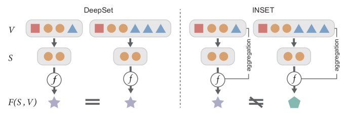
Figure 1: (Left): The DeepSet-style models only focus on processing the subset $S$. (Right): In contrast, INSET not only identifies the subset $S$ but also takes the identification of $V$ into account, which parameterizes the information that $S$ is a subset of $V$ during the training process.

To address these challenges, our research focuses on the aggregation of background information from the superset $V$ into the subset $S$ from a symmetric perspective. Initially, we describe the symmetry group of $(S,V)$ during neural subset selection, as outlined in Section 3.2. Specifically, the subset $S$ is required to fulfill permutation symmetry, while the superset $V$ needs to satisfy a corresponding symmetry group within the nested sets scheme. We denote this hierarchical symmetry of $(S,V)$ as $\mathcal{G}$. Subsequently, we theoretically investigate the connection between functional symmetry and probabilistic symmetry within $F(S,V)$ and $P(Y|S,V)$, indicating that the conditional distribution can be utilized to construct a neural network that processes the invariant sufficient representation of $(S,V)$ with respect to $\mathcal{G}$. These representations, defined in Section 3.3, are proven to satisfy Sufficiency and Adequacy, which means such representations retain the information of the prediction $Y$ while disregarding the order of the elements in $S$ or $V$. Building upon the above theoretical results, we propose an interpretable and powerful model called INSET (Invariant Representation of Subsets) for neural subset selection in Section 3.4. INSET incorporates an information aggregation step between the invariant sufficient representations of $S$ and $V$, as illustrated in Figure 1. This ensures that the model’s output can approximate the relationship between $Y$ and $(S,V)$ while being unaffected by the transformations of $\mathcal{G}$. Furthermore, in contrast to previous works that often disregard the information embedded within the set $V$, our exceptional model (INSET) excels in identifying the superset $V$ from which the subset $S$ originates.

In summary, we makes the following contributions. Firstly, we approach neural set selection from a symmetric perspective and establish the connection between functional symmetry and probabilistic symmetry in $P(Y|S,V)$, which enables us to characterize the model structure. Secondly, we introduce INSET, an effective and interpretable approach model for neural subset selection. Lastly, we empirically validate the effectiveness of INSET through comprehensive experiments on diverse datasets, encompassing tasks such as product recommendation, set anomaly detection, and compound selection, achieving up to $23\%$ improvement in Mean Jaccard Coefficient (MJC) evaluated on the set anomaly detection task.

2 Related Work

Encoding Interactions for Set Representations. Designing network architectures for set-structured input has emerged as a highly popular research topic. Several prominent works, including those (Ravanbakhsh et al., 2017; Edwards & Storkey, 2016; Zaheer et al., 2017; Qi et al., 2017a; Horn et al., 2020; Bloem-Reddy & Teh, 2020) have focused on constructing permutation equivariant models using standard feed-forward neural networks. These models demonstrate the ability to universally approximate continuous permutation-invariant functions through the utilization of set-pooling layers. However, existing approaches solely address the representation learning at the set level and overlook interactions within sub-levels, such as those between elements and subsets.

Motivated by this limitation, subsequent studies have proposed methods to incorporate richer interactions when modeling invariant set functions for different tasks. For instance, (Lee et al., 2019b) introduced the use of self-attention mechanisms to process elements within input sets, naturally capturing pairwise interactions. Murphy et al. (2018) proposed Janossy pooling as a means to encode higher-order interactions within the pooling operation. Further improvements have been proposed by (Kim, 2021; Li et al., 2020), among others. Additionally, Bruno et al. (2021); Willette et al. (2022) developed techniques to ensure Mini-Batch Consistency in set encoding, enabling the provable equivalence between mini-batch encodings and full set encodings by leveraging interactions. These studies emphasize the significance of incorporating interactions between different components.

Information-Sharing in Neural Networks. In addition to set learning tasks, the interaction between different components holds significance across various data types and neural networks. Recent years have witnessed the development of several deep neural network-based methods that explore hierarchical structures. For Convolutional Neural Networks (CNNs), various hierarchical modules have been proposed by Deng et al. (2014); Murthy et al. (2016); Xiao et al. (2014); Chen et al. (2020); Ren et al. (2020; 2019) to address different image-related tasks. In the context of graph-based tasks, (Defferrard et al., 2016; Cangea et al., 2018; Gao & Ji, 2019; Ying et al., 2018b; Huang et al., 2019; Ying et al., 2018a; Jin et al., 2020; Han et al., 2022), and others have put forth different methods to learn hierarchical representations. The focus of these works lies in capturing local information effectively and integrating it with global information.

However, the above works ignore the symmetry and expressive power in designing models. Motivated by this, Maron et al. (2020); Wang et al. (2020) proposed how to design linear equivariant and invariant layers for learning hierarchical symmetries to handle per-element symmetries. Moreover, there are some works proposed for different tasks considering symmetry and hierarchical structure, e.g., (Han et al., 2022; Ganea et al., 2022). Our method differs from previous work by focusing on generating a subset $S\in V$ as the final output, rather than output the entire set $V$. Besides, INSET embraces a probabilistic perspective, aligning with the nature of the Optimal Subset (OS) oracle.

3 Method

3.1 Background

Let’s consider the ground set composed of $n$ elements, denoted as $x_{i}$, i.e., $V=\{x_{1},x_{2},...,x_{n}\}$. In order to facilitate the proposition of Property 3.1, we describe $V$ as a collection of several disjoint subsets, specifically $V=\{S_{1},\dots,S_{m}\}$, where $S_{i}\in\mathbb{R}^{n_{i}\times d}$. Here, $n_{i}$ represents the size of subset $S_{i}$, and each element $x_{i}\in{\mathcal{X}}$ is represented by a $d$-dimensional tensor. It is worth noting that, without loss of generality, we can treat $S_{i}$ as individual elements, i.e., $n_{i}=1$. As an example of neural subset selection, the task involves encoding subsets $S_{i}$ into representative vectors to predict the corresponding function value $Y\in{\mathcal{Y}}$, as discussed in the introduction section. Existing methods such as (Zaheer et al., 2017) and (Ou et al., 2022) directly select $S_{i}$ from the encoding embeddings of all elements in $V$, and then input $S_{i}$ into feed-forward networks. However, these methods approximate the function $F(S_{i},V)$ using only the explicit subsets $S_{i}$, which can be suboptimal since the function also relies on information from the ground set $V$. Furthermore, this approach leads to a conditional distribution $P(Y|S)$ instead of the desired $P(Y|S,V)$. Throughout this study, we assume that all random variables take values in standard Borel spaces, and all introduced maps are measurable.

In this section, we introduce a principled approach for encoding subset representations that leverages background information from the entire input set $V$ to achieve better performance. Additionally, our theoretical results naturally align with the task of neural subset selection in OS Oracle, as they focus on investigating the probabilistic relationship between $Y$ and $(S,Y),$ which also establishes a connection between the conditional distribution and the functional representation of both $S$ and $V$. By linking the functional representation to the conditional distribution, our results also provide insights into constructing a neural network that effectively approximates the desired function $F(S,V)$.

3.2 The Symmetric Information from Supersets

When considering the invariant representation of $S$ alone, we can directly utilize DeepSets with a max-pooling operation. However, incorporating background information from $V$ into the representations poses the challenge of determining the appropriate inductive bias for the modeling process. One straightforward approach is to assume the existence of two permutation groups that act independently on $V$ and $S$. However, this assumption is impractical since $S$ is a part of $V$. If we transform $S$, the corresponding adjustments should also be made to $V$. From the perspective of the interaction between subsets and supersets, a natural consideration is to view the supersets as a nested set of sets, i.e., $V=S_{1}\cup S_{2}\cup\dots\cup S_{m},$ where $S_{i}\cap S_{j}=\emptyset$ if $i\neq j$. In this perspective, the symmetric properties will become more evident.

We assume the presence of an outer permutation $\pi_{m}\in\mathbb{S}_{m}$ that maps indices of the subsets to new indices, resulting in a reordering of the subsets within $V$. Furthermore, within each subset $S_{i}$, there exists a permutation group denoted by $h_{i}\in{\mathcal{H}}_{i}$, which captures the possible rearrangements of elements within that specific subset. Each element of $h_{i}$ represents a distinct permutation on the elements of $S_{i}$. The symmetry of nested sets of sets, referred to as ${\mathcal{R}}$, can be defined as the wreath product of the symmetric group $\mathbb{S}_{m}$ (representing outer permutations on the $m$ subsets) and the direct product of the permutation groups associated with each subset (${\mathcal{G}}_{1}\times{\mathcal{G}}_{2}\times\dots\times{\mathcal{G}}_{m}$). Formally, ${\mathcal{R}}=S_{m}\wr({\mathcal{G}}_{1}\times{\mathcal{G}}_{2}\times\dots\times{\mathcal{G}}_{m})$. Therefore, for any transformation $r\in{\mathcal{R}}$ acting on $V$, there must exist a corresponding $h\in{\mathcal{H}}$ acting on $S$. Keeping this in mind, we define the conditional distribution $P(Y|S,V)$ to adhere to the following property:

Property 3.1.

Let $S\in{\mathcal{S}},V\in{\mathcal{V}}$ and $Y\in{\mathcal{Y}},$ where ${\mathcal{H}}$ and ${\mathcal{R}}$ act on ${\mathcal{S}}$ and ${\mathcal{V}},$ respectively. Then, the conditional distribution $P(Y|S,V)$ of $Y$ give $(S,V)$ is said to be invariant under a group ${\mathcal{H}}$ and ${\mathcal{R}}$ if and only if:

$$P(Y\mid S,V)=P(Y\mid g\cdot(S,V))=P(Y\mid h\cdot S,r\cdot V)\quad\text{for any }h\in{\mathcal{H}}\quad\text{and}\quad r\in{\mathcal{R}}\;.$$

In this context, we denote the composite group $\mathcal{G}={\mathcal{H}}\times{\mathcal{R}}$, which acts on the product space $S\times V$. We have now clarified the specific inductive bias that should be considered when characterizing neural networks. In the subsequent subsection, we will delve into the exploration of constructing neural networks that fulfill this property.

3.3 Invariant Sufficient Representation

Functional and probabilistic notions of symmetries represent two different approaches to achieving the same goal: a principled framework for constructing models from symmetry considerations. To characterize the precise structure of the neural network satisfying Property 3.1, we need to use a technical tool, that transfers a conditional probability distribution $P(Y|S,V)$ into a representation of $Y$ as a function of statics of $(S,V)$ and random noise, i.e., $f(\xi,M(S,V))$. Here, $M$ are maps, which are based on the idea that a statistic may contain all the information that is needed for an inferential procedure. There are mainly two terms as Sufficiency and Adequacy. The ideas go hand-in-hand with notions of symmetry: while invariance describes information that is irrelevant, sufficiency and adequacy describe the information that is relevant.

There are various methods to describe sufficiency and adequacy, which are equivalent under some constraints. For convenience and completeness, we follow the concept from (Halmos & Savage, 1949; Bloem-Reddy & Teh, 2020). We begin by defining the sufficient statistic as follows, where ${\mathcal{B}}_{{\mathcal{X}}}$ represents the Borel $\sigma$-algebra of ${\mathcal{X}}$:

Definition 3.2.

Assume $M:{\mathcal{S}}\times{\mathcal{V}}\to{\mathcal{M}}$ a measurable map and there is a Markov kernel $k:{\mathcal{B}}_{{\mathcal{X}}}\times{\mathcal{S}}\times{\mathcal{V}}\to\mathbb{R}_{+}$ such that for all $X\in{\mathcal{X}}$ and $m\in{\mathcal{M}}$, $P({\,\vbox{\hbox{\scalebox{0.75}{$\bullet$}}}\,}\mid M(S,V)=m)=k({\,\vbox{\hbox{\scalebox{0.75}{$\bullet$}}}\,},m)$. Then $M$ is a sufficient statistic for $P(S,V).$

This definition characterizes the information pertaining to the distribution of $(S,V)$. More specifically, it signifies that there exists a single Markov kernel that yields the same conditional distribution of $(S,V)$ conditioned on $M(S,V)=m$, regardless of the distribution $P(S,V)$. It is important to note that if $S\nsubseteq V$, the corresponding value of $M(S,V)$ would be zero, which is an invalid case. When examining the distribution of $Y$ conditioned on $S$ and $V$, an additional definition is required:

Definition 3.3.

Let $M:{\mathcal{S}}\times{\mathcal{V}}\to{\mathcal{M}}$ be a measurable map and assume $M$ is sufficient for $P(S,V)$. If for all $s\in{\mathcal{S}},$ $v\in{\mathcal{V}}$ and $y\in{\mathcal{Y}},$

$$P(Y\in{\,\vbox{\hbox{\scalebox{0.75}{$\bullet$}}}\,}\mid S=s,V=v)=P(Y\in{\,\vbox{\hbox{\scalebox{0.75}{$\bullet$}}}\,}\mid M(S,V)=m)\,.$$ (2)

Then, $M$ serves as an adequate statistic of $(S,V)$ for $Y$, and also acts as the sufficient statistic.

Actually, Equation (2) is equivalent to conditional independence of $Y$ and $(S,V)$, given $M(S,V),$ i.e., $Y{\perp\!\!\!\perp}_{M(X)}X,$ This is also called $M$ d-separates $(S,V)$ and $Y.$ In other words, if our goal is to approximate the invariant conditional distribution $P(Y|S,V)$, we can first seek an invariant representation of $(S,V)$ under $\mathcal{G}$, which also acts as an adequate statistic for $(S,V)$ with respect to $Y$. Consequently, modeling the relationship between $(S,V)$ and $Y$ directly is equivalent to learning the relationship between $M(S,V)$ and $Y$, which naturally satisfies Property 3.1.

With the given definitions, it becomes evident that we can discover an invariant representation of $(S,V)$ with respect to the symmetric groups $\mathcal{G}$. This representation is referred to as the Invariant Sufficient Representation, signifying that an invariant effective representation should eliminate the information influenced by the actions of $\mathcal{G}$, while preserving the remaining information regarding its distribution. This concept is also referred to as Maximal Invariant in some previous literature, such as (Kallenberg et al., 2017; Bloem-Reddy & Teh, 2020).

Definition 3.4.

(Invariant Sufficient Representation) For a group $\mathcal{G}$ of actions on any $(s,v)\in{\mathcal{S}}\times{\mathcal{V}}$ , we say $M:{\mathcal{S}}\times{\mathcal{V}}\to{\mathcal{M}}$ is a invariant sufficient representation for space ${\mathcal{S}}\times{\mathcal{V}}$, if it satisfies: If $M(s_{1},v_{1})=M(s_{2},v_{2})$, then $(s_{2},v_{2})=g\cdot(s_{1},v_{1})$ for some $g\in\mathcal{G}$; otherwise, there is no such $g$ that satisfies $(s_{2},v_{2})=g\cdot(s_{1},v_{1})$.

Clearly, the invariant sufficient representation $M$ serves as the sufficient statistic for $(S,V)$. Furthermore, if the conditional distribution $P(Y|S,V)$ is invariant to transformations induced by the group $\mathcal{G}$, we can establish that $M(S,V)$ is an adequate statistic for $(S,V)$, as stated in Corollary 3.6. In other words, $M(S,V)$ can be considered to encompass all the relevant information for predicting the label given $(S,V)$ while eliminating the redundant information about $\mathcal{G}$. Hence, we can construct models that learn the relationship between $M(S,V)$ and $Y$, ultimately resulting in an invariant function $Y=f(S,V)$ under the group $\mathcal{G}$. From a probabilistic standpoint, this implies that $P(Y|S,V)=P(Y|M(S,V))$.

3.4 Characterizing the Model Structure

Hence, by computing the invariant sufficient representations of $(S,V)$, we can construct a $\mathcal{G}$-invariant layer. This idea can give rise to the following theorem:

Theorem 3.5.

Consider a measurable group $\mathcal{G}$ acting on ${\mathcal{S}}\times{\mathcal{V}}$. Suppose we select an invariant sufficient representation denoted as $M:{\mathcal{S}}\times{\mathcal{V}}\to{\mathcal{M}}$. In this case, $P(Y|S,V)$ satisfies Property 3.1 if and only if there exists a measurable function denoted as $f:[0,1]\times{\mathcal{S}}\times{\mathcal{V}}\to{\mathcal{Y}}$ such that the following equation holds:

$$(S,V,Y)=_{\text{\rm a.s.}}\big{(}S,V,f(\xi,M(S,V))\big{)}\quad\text{where }\xi\sim\text{\rm Unif}[0,1]\text{ and }\xi{\perp\!\!\!\perp}(S,V);.$$ (3)

In this context, the variable $\xi$ represents generic noise, which can be disregarded when focusing solely on the model structure rather than the complete training framework (Bloem-Reddy & Teh, 2020; Ou et al., 2022). Consequently, the theorem highlights the necessity of characterizing the neural networks in the form of $f(M(S,V))$. Moreover, Theorem 3.5 implies that the invariant sufficient representation $M(S,V)$ also serves as an adequate statistic. This can be illustrated as follows:

$$P(Y\in{\,\vbox{\hbox{\scalebox{0.75}{$\bullet$}}}\,}|S=s,V=v)=P(Y\in{\,\vbox{\hbox{\scalebox{0.75}{$\bullet$}}}\,}|S=s,V=v,M(S,V)=m)=P(Y\in{\,\vbox{\hbox{\scalebox{0.75}{$\bullet$}}}\,}|M(S,V)=m).$$

To provide additional precision and clarity, we present the following corollary, which demonstrates that $M(S,V)$ is an adequate statistic of $(S,V)$ for $Y.$

Corollary 3.6.

Let $\mathcal{G}$ be a compact group acting measurably on standard Borel spaces $S\times V$, and let ${\mathcal{M}}$ be another Borel space. Then Any invariant sufficient representation $M:{\mathcal{S}}\times{\mathcal{V}}\to{\mathcal{M}}$ under $\mathcal{G}$ is an adequate statistic of $(S,V)$ for $Y.$

3.5 Implementation

In theory, invariant sufficient representations can be computed by selecting a representative element for each orbit under the group $\mathcal{G}$. However, this approach is impractical due to the high dimensions of the input space and the potentially enormous number of orbits. Instead, in practice, a neural network can be employed to approximate this process and generate the desired representations (Zaheer et al., 2017; Bloem-Reddy & Teh, 2020), particularly in tasks involving sets or set-like structures.

However, the approach to approximating such a representation for $(S,V)$ under $\mathcal{G}$ remains unclear. To simplify the problem, we can divide the task of finding the invariant sufficient representation of $S$ and $V$ under $H$ and $R$, respectively, as defined in Section 3.2. This concept is guaranteed by the following proposition:

Proposition 3.7.

Assuming that $M_{s}:\mathcal{S}\to\mathcal{S}_{1}$ and $M_{v}:\mathcal{V}\to\mathcal{V}_{1}$ serve as invariant sufficient representations for $S$ and $V$ with respect to $H$ and $R$, respectively, then there exist maps $f:\mathcal{S}_{1}\times\mathcal{V}_{1}\to\mathcal{M}$ that establish the invariant sufficient representation of $M$.

Proposition 3.7 specifically states that we can construct the invariant sufficient representations for $S$ and $V$ individually, as they are comparatively easier to construct compared to $M(S,V)$. In the work of (Bloem-Reddy & Teh, 2020), it is demonstrated that for $S$ under $H$, the empirical measure $M_{s}(S)=\sum_{s_{i}\in S}\delta(s_{i})$ can be chosen as a suitable invariant sufficient representation. Here, $\delta(s_{i})$ represents an atom of unit mass located at $s_{i}$, such as one-hot embeddings. Additionally, leveraging the proposition established by Zaheer et al. (2017), we can employ $\rho\sum_{s\in S}\phi(s)$ to approximate the empirical measure. This approximation offers a practical and effective approach to constructing the invariant sufficient representation.

Proposition 3.8.

If $f$ is a valid permutation invariant function on $S$, it can be approximated arbitrarily close in the form of $f(S)=\rho\left(\sum_{s\in S}\phi(s)\right)$, for suitable transformations $\phi$ and $\rho$.

During the implementation, an encoder $\phi$ is utilized to generate embeddings for each element. For example, when dealing with sets of images, ResNet can be employed as the encoder. On the other hand, $\rho$ can represent various feedforward networks, such as fully connected layers combined with nonlinear activation functions. Similarly, for the symmetric group ${\mathcal{R}}$ acting on $V$, Maron et al. (2020) has demonstrated that the universal approximators of the invariant sufficient representations are $\sum_{S\in V}\sum_{s\in S}\phi(s)$, which is equivalent to $\sum_{x_{j}\in V}\phi(x_{j})$. Hence, for neural subset selection tasks, when considering a specific subset $S\in V$, The neural network construction is outlined as follows:

$$\theta(S,V)=\sigma\bigg{(}\theta_{1}(\sum_{i=1}^{n_{i}}\phi(x_{i}))+\theta_{2}\bigg{(}\sum_{i=1}^{n}\phi(x_{j})\bigg{)}\bigg{)},$$ (4)

Here, the feed-forward modules $\theta_{1}$ and $\theta_{2}$ are accompanied by a non-linear activation layer denoted by $\sigma$. Intuitively, the inherent simplicity of the structure enables us to utilize the DeepSet module to process all elements in $V$ and integrate them with the invariant sufficient representations of $S.$ In Appendix LABEL:sec:app:cost, we provided an illustration of such a structure in Figure LABEL:fig:structure and a description of DeepSet. In practice, there are different ways to integrate the representation of $V$ into the representation of $S$, such as concatenation (Qi et al., 2017a) or addition (Maron et al., 2020). Although this idea is straightforward, in the following section, we will demonstrate how this modification significantly enhances the performance of baseline methods. Notably, this idea has been empirically utilized in previous works, such as (Qi et al., 2017a; b). However, we propose it from a probabilistic invariant perspective. A corresponding equivariant framework was also introduced in Wang et al. (2020), which complements our results in the development of deep equivariant neural networks.

4 Experiments

The proposed methods are assessed across multiple tasks, including product recommendation, set anomaly detection, and compound selection. To ensure robustness, all experiments are repeated five times using different random seeds, and the means and standard deviations of the results are reported. For additional experimental details and settings, we provide comprehensive information in Appendix LABEL:sec:app:exp.

Evaluations. The main goal of the following tasks is to predict the corresponding $S^{\star}$ given $V.$ Therefore, we evaluate the methods using the mean Jaccard coefficient (MJC) metric. Specifically, for each data sample $(S^{\star},V)$ if the model’s prediction is $S^{\prime},$ then the Jaccard coefficient is given as: $JC(S^{\star},S^{\prime})=\frac{|S^{\star}\cap S^{\prime}|}{|S^{\star}\cup S^{\prime}|}.$ Therefore, the MJC is computed by averaging JC metric over all samples in the test set.

Baselines. To show our method can achieve better performance on real applications, we compare it with the following methods:

• Random. The results are calculated based on random estimates, which provide a measure of how challenging the tasks are.

• PGM (Tschiatschek et al., 2018). PGM is a probabilistic greedy model (PGM) solves optimization Problem 1 with a differentiable extension of greedy maximization algorithm. Further detailed information can be found in Appendix LABEL:sec:app:pgm.

• DeepSet (Zaheer et al., 2017). Here, we use DeepSet as a baseline by predicting the probability of which instance should be in $S^{\star},$ i.e., learn an invariant permutation mapping $2^{V}\mapsto[0,1]^{|V|}$. It serves as the backbone in EquiVSet to learn set functions, and can also be employed as a baseline.

• Set Transformer (Lee et al., 2019a). Set Transformer, compared with DeepSet, goes beyond by incorporating the self-attention mechanism to account for pairwise interactions among elements. This will make models to capture dependencies and relationships between different elements.

• EquiVSet (Ou et al., 2022). EquiVSet uses an energy-based model (EBM) to construct the set mass function $P(S|V)$ from a probabilistic perspective, i.e, they mainly focus on learning a distribution $P(S|V)$ monotonically growing with the utility function $F(S,V).$ This requires to learn a conditional distribution $P(Y|S,V)$ as approximation distribution. Actually, their framework is to approximate symmetric $F(S)$ instead of symmetric $F(S,V),$ and they use DeepSet as their backbone.

Table 1: Product recommendation results on all categories.

Categories	Random	PGM	DeepSet	Set Transformer	EquiVSet	INSET
Toys	0.083	0.441 $\pm$ 0.004	0.421 $\pm$ 0.005	0.625 $\pm$ 0.020	0.684 $\pm$ 0.004	0.769 $\pm$ 0.005
Furniture	0.065	0.175 $\pm$ 0.007	0.168 $\pm$ 0.002	0.176 $\pm$ 0.008	0.162 $\pm$ 0.020	0.169 $\pm$ 0.050
Gear	0.077	0.471 $\pm$ 0.004	0.379 $\pm$ 0.005	0.647 $\pm$ 0.006	0.725 $\pm$ 0.011	0.808 $\pm$ 0.012
Carseats	0.066	0.230 $\pm$ 0.010	0.212 $\pm$ 0.008	0.220 $\pm$ 0.010	0.223 $\pm$ 0.019	0.231 $\pm$ 0.034
Bath	0.076	0.564 $\pm$ 0.008	0.418 $\pm$ 0.007	0.716 $\pm$ 0.005	0.764 $\pm$ 0.020	0.862 $\pm$ 0.005
Health	0.076	0.449 $\pm$ 0.002	0.452 $\pm$ 0.001	0.690 $\pm$ 0.010	0.705 $\pm$ 0.009	0.812 $\pm$ 0.005
Diaper	0.084	0.580 $\pm$ 0.009	0.451 $\pm$ 0.003	0.789 $\pm$ 0.005	0.828 $\pm$ 0.007	0.880 $\pm$ 0.007
Bedding	0.079	0.480 $\pm$ 0.006	0.481 $\pm$ 0.002	0.760 $\pm$ 0.020	0.762 $\pm$ 0.005	0.857 $\pm$ 0.010
Safety	0.065	0.250 $\pm$ 0.006	0.221 $\pm$ 0.004	0.234 $\pm$ 0.009	0.230 $\pm$ 0.030	0.238 $\pm$ 0.015
Feeding	0.093	0.560 $\pm$ 0.008	0.428 $\pm$ 0.002	0.753 $\pm$ 0.006	0.819 $\pm$ 0.009	0.885 $\pm$ 0.005
Apparel	0.090	0.533 $\pm$ 0.005	0.508 $\pm$ 0.004	0.680 $\pm$ 0.020	0.764 $\pm$ 0.005	0.837 $\pm$ 0.003
Media	0.094	0.441 $\pm$ 0.009	0.426 $\pm$ 0.004	0.530 $\pm$ 0.020	0.554 $\pm$ 0.005	0.620 $\pm$ 0.023

4.1 Product Recommendation

The task requires models to recommend the most interested subset for a customer given 30 products in a category. We use the dataset (Gillenwater et al., 2014) from the Amazon baby registry for this experiment, which includes many product subsets chosen by various customers. Amazon classifies each item on a baby registry as being under one of several categories, such as “Health” and “Feeding”. Moreover, each product is encoded into a 768-dimensional vector by the pre-trained BERT model based on its textual description. Table 1 reports the performance of all the models across different categories. Out of the twelve cases evaluated, INSET performs best in ten of them, except for Furniture and Safety tasks. The discrepancy in performance can be attributed to the fact that our method is built upon the EquiVSet framework, with the main modification being the model structure for modeling $F(S,V)$. Consequently, when EquiVSet performs poorly, it also affects the performance of INSET. Nonetheless, it is worth noting that INSET consistently outperforms EquiVSet and achieves significantly better results than other baselines in the majority of cases. The margin of improvement is substantial, demonstrating the effectiveness and superiority of INSET.

4.2 Set Anomaly Detection

We conduct set anomaly detection tasks on three real-world datasets: the double MNIST (Sun, 2019), the CelebA (Liu et al., 2015b) and the F-MNIST (Xiao et al., 2017). Each dataset is divided into the training, validation, and test sets with sizes of 10,000, 1,000, and 1,000, respectively. For each dataset, we randomly sample $n\in\{2,3,4\}$ images as the OS oracle $S^{*}.$ The setting is followed by (Zaheer et al., 2017; Ou et al., 2022). Let’s take CelebA as an example. In this case, the objective is to identify anomalous faces within each set solely through visual observation, without any access to attribute values. The CelebA dataset comprises 202,599 face images, each annotated with 40 boolean attributes. When constructing sets, for every ground set $V$, we randomly choose n images from the dataset to form the OS Oracle $S^{*}$, ensuring that none of the selected images contain any of the two attributes. Additionally, it is ensured that no individual person’s face appears in both the training and test sets. Regarding Table 2, it is evident that our model demonstrates a substantial performance advantage over all the baselines. Specifically, in the case of Double MNIST, our model shows a remarkable improvement of 23% compared to EquiVSet, which itself exhibits the best performance among all the baselines considered. This significant margin of improvement highlights the superior capabilities of our model in tackling the given task.

Table 2: Set anomaly detection and compound selection results

	Anomaly Detection			Compound selection
	Double MNIST	CelebA	F-MNIST	PDBBind	BindingDB
Random	0.0816	0.2187	0.193	0.099	0.009
PGM	0.300 $\pm$ 0.010	0.481 $\pm$ 0.006	0.540 $\pm$ 0.020	0.910 $\pm$ 0.010	0.690 $\pm$ 0.020
DeepSet	0.111 $\pm$ 0.003	0.440 $\pm$ 0.006	0.490 $\pm$ 0.020	0.901 $\pm$ 0.011	0.710 $\pm$ 0.020
Set Transformer	0.512 $\pm$ 0.005	0.527 $\pm$ 0.008	0.581 $\pm$ 0.010	0.919 $\pm$ 0.015	0.715 $\pm$ 0.010
EquiVSet	0.575 $\pm$ 0.018	0.549 $\pm$ 0.005	0.650 $\pm$ 0.010	0.924 $\pm$ 0.011	0.721 $\pm$ 0.009
INSET	0.707 $\pm$ 0.010	0.580 $\pm$ 0.012	0.721 $\pm$ 0.021	0.935 $\pm$ 0.008	0.734 $\pm$ 0.010

4.3 Compound Selection in AI-aided Drug Discovery

The screening of compounds with diverse biological activities and satisfactory ADME (absorption, distribution, metabolism, and excretion) properties is a crucial stage in drug discovery tasks (Li et al., 2021; Ji et al., 2022; Gimeno et al., 2019). Consequently, virtual screening is often a sequential filtering procedure with numerous necessary filters, such as selecting diverse subsets from the highly active compounds first and then removing compounds that are harmful for ADME. After several filtering stages, we reach the optimal compound subset. However, it is hard for neural networks to learn the full screening process due to a lack of intermediate supervision signals, which can be very expensive or impossible to obtain due to the pharmacy’s protection policy. Therefore, the models are supposed to learn this complicated selection process in an end-to-end manner, i.e., models will predict $S^{*}$ only given the optimal subset supervision signals without knowing the intermediate process. However, this is out of the scope of this paper, since the task is much more complex and requires extra knowledge, and thus we leave it as future work.

Table 3: Ablation Studies on CelebA with different parameters

	MJC	Parameters
Random	0.2187	-
EquiVSet	0.549$\pm$0.005	1782680
EquiVSet (v1)	0.554$\pm$0.007	2045080
EquiVSet (v2)	0.560$\pm$0.005	3421592
INSET	0.580$\pm$0.012	2162181

To simulate the process, we only apply one filter: high bioactivity to acquire the optimal subset of compound selection following (Ou et al., 2022). We conduct experiments using the following datasets: PDBBind (Liu et al., 2015a) and BindingDB (Liu et al., 2007). Table 2 shows that our method performs better than the baselines and significantly outperform the random guess, especially on the BindingDB dataset. Different from the previous tasks, the performance of these methods is closer to each other. That is because the structure of complexes (the elements in a set) can provide much information for this task. Thus, the model could predict the activity value of complexes well without considering the interactions between the optimal subset and the complementary. However, our method can still achieve more satisfactory results than the other methods.

4.4 Computation Cost

The main difference between INSET and EquiVSet is the additional information-sharing module to incorporate the representations of $V$. A possible concern is that the better performance of INSET might come from the extra parameters instead of our framework proposed. To address this concern, we conducted experiments on CelebA datasets. We add an additional convolution layer in the encoders to improve the capacity of EquiVSet. According to the location and size, we propose two variants of EquiVSet, details can be found in the appendix. We report the performance of models with different model sizes in Table 3. It is evident that INSET surpasses all the variants of EquiVSet, clearly demonstrating superior performance. Notably, the improvement achieved through the parameters is considerably less significant when compared to the substantial improvement resulting from the information aggregation process. This highlights the crucial role of information aggregation in driving the overall performance enhancement of INSET.

4.5 Performance versus Training Epochs

In addition to the notable improvement in the final MJC achieved by INSET, we have also observed that incorporating more information from the superset leads to enhanced training speed and better overall performance. To illustrate this, we present two figures depicting the validation performance against the number of training epochs for the Toys and Diaper datasets. It is evident that INSET achieves favorable performance in fewer training epochs. For instance, on the Toy dataset, INSET reaches the best performance of EquiVSet, at approximately epoch 18. Furthermore, around epoch 25, INSET approaches its optimal performance, while EquiVSet and Set Transformer attain their best performance around epoch 40. This highlights the efficiency and effectiveness of INSET in achieving competitive results within a shorter training time.

5 Conclusion

In this study, we have identified a significant limitation in subset encoding methods, such as neural subset selection, where the output is either the subset itself or a function value associated with the subset. By incorporating the concept of permutation invariance, we reformulate this problem as the modeling of a conditional distribution $P(Y|S,V)$ that adheres to Property 3.1. Our theoretical analysis further reveals that to accomplish this objective, it is essential to construct a neural network based on the invariant sufficient representation of both $S$ and $V$. In response, we introduce INSET, a highly accurate and theoretical-driven approach for neural subset selection, which also consistently outperforms previous methods according to empirical evaluations.

Limitations and Future Work. INSET is a simple yet effective method in terms of implementation, indicating that there is still potential for further improvement by integrating additional information, such as pairwise interactions between elements. Furthermore, our theoretical analysis is not limited to set-based tasks; it can be applied to more general scenarios with expanded definitions and theoretical contributions. We acknowledge that these potential enhancements and extensions are left as future work, offering opportunities for further exploration and development.

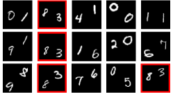
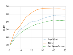
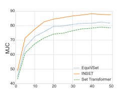
Figure 2: Left: A sample from the Double MNIST dataset, comprising $|S^{*}|$ images displaying the same digit (indicated by the red box). Right: The two figures on the right display the validation performance plotted against the number of epochs for Toys and Diaper datasets, respectively. The x-axis represents the epochs.

References

- Balcan & Harvey (2018) Maria-Florina Balcan and Nicholas J. A. Harvey. Submodular functions: Learnability, structure, and optimization. SIAM J. Comput., 47(3):703–754, 2018.
- Bloem-Reddy & Teh (2020) Benjamin Bloem-Reddy and Yee Whye Teh. Probabilistic symmetries and invariant neural networks. J. Mach. Learn. Res., 21:90:1–90:61, 2020.
- Bruno et al. (2021) Andreis Bruno, Jeffrey Willette, Juho Lee, and Sung Ju Hwang. Mini-batch consistent slot set encoder for scalable set encoding. Advances in Neural Information Processing Systems, 34:21365–21374, 2021.
- Cangea et al. (2018) Cătălina Cangea, Petar Veličković, Nikola Jovanović, Thomas Kipf, and Pietro Liò. Towards sparse hierarchical graph classifiers. arXiv preprint arXiv:1811.01287, 2018.
- Chen et al. (2020) Cen Chen, Xiaofeng Zou, Zeng Zeng, Zhongyao Cheng, Le Zhang, and Steven CH Hoi. Exploring structural knowledge for automated visual inspection of moving trains. IEEE transactions on cybernetics, 2020.
- Defferrard et al. (2016) Michaël Defferrard, Xavier Bresson, and Pierre Vandergheynst. Convolutional neural networks on graphs with fast localized spectral filtering. Advances in neural information processing systems, 29:3844–3852, 2016.
- Deng et al. (2014) Jia Deng, Nan Ding, Yangqing Jia, Andrea Frome, Kevin Murphy, Samy Bengio, Yuan Li, Hartmut Neven, and Hartwig Adam. Large-scale object classification using label relation graphs. In European conference on computer vision, pp. 48–64. Springer, 2014.
- Edwards & Storkey (2016) Harrison Edwards and Amos Storkey. Towards a neural statistician. arXiv preprint arXiv:1606.02185, 2016.
- Ganea et al. (2022) Octavian-Eugen Ganea, Xinyuan Huang, Charlotte Bunne, Yatao Bian, Regina Barzilay, Tommi S. Jaakkola, and Andreas Krause. Independent SE(3)-equivariant models for end-to-end rigid protein docking. In International Conference on Learning Representations, 2022.
- Gao & Ji (2019) Hongyang Gao and Shuiwang Ji. Graph u-nets. In international conference on machine learning, pp. 2083–2092. PMLR, 2019.
- Gillenwater et al. (2014) Jennifer Gillenwater, Alex Kulesza, Emily B. Fox, and Benjamin Taskar. Expectation-maximization for learning determinantal point processes. In Advances in Neural Information Processing Systems 27: Annual Conference on Neural Information Processing Systems 2014, December 8-13 2014, Montreal, Quebec, Canada, pp. 3149–3157, 2014.
- Gimeno et al. (2019) Aleix Gimeno, María José Ojeda-Montes, Sarah Tomás-Hernández, Adrià Cereto-Massagué, Raúl Beltrán-Debón, Miquel Mulero, Gerard Pujadas, and Santiago Garcia-Vallvé. The light and dark sides of virtual screening: what is there to know? International journal of molecular sciences, 20(6):1375, 2019.
- Halmos & Savage (1949) Paul R Halmos and Leonard J Savage. Application of the radon-nikodym theorem to the theory of sufficient statistics. The Annals of Mathematical Statistics, 20(2):225–241, 1949.
- Han et al. (2022) Jiaqi Han, Yu Rong, Tingyang Xu, Fuchun Sun, and Wenbing Huang. Equivariant graph hierarchy-based neural networks. arXiv preprint arXiv:2202.10643, 2022.
- Horn et al. (2020) Max Horn, Michael Moor, Christian Bock, Bastian Rieck, and Karsten Borgwardt. Set functions for time series. In Hal Daumé III and Aarti Singh (eds.), Proceedings of the 37th International Conference on Machine Learning, volume 119 of Proceedings of Machine Learning Research, pp. 4353–4363. PMLR, 13–18 Jul 2020.
- Huang et al. (2019) Jingjia Huang, Zhangheng Li, Nannan Li, Shan Liu, and Ge Li. Attpool: Towards hierarchical feature representation in graph convolutional networks via attention mechanism. In 2019 IEEE/CVF International Conference on Computer Vision (ICCV), pp. 6479–6488, 2019.
- Ji et al. (2022) Yuanfeng Ji, Lu Zhang, Jiaxiang Wu, Bingzhe Wu, Long-Kai Huang, Tingyang Xu, Yu Rong, Lanqing Li, Jie Ren, Ding Xue, Houtim Lai, Shaoyong Xu, Jing Feng, Wei Liu, Ping Luo, Shuigeng Zhou, Junzhou Huang, Peilin Zhao, and Yatao Bian. Drugood: Out-of-distribution (OOD) dataset curator and benchmark for ai-aided drug discovery - A focus on affinity prediction problems with noise annotations. CoRR, abs/2201.09637, 2022.
- Jin et al. (2020) Wengong Jin, Regina Barzilay, and Tommi Jaakkola. Hierarchical generation of molecular graphs using structural motifs. In International conference on machine learning, pp. 4839–4848. PMLR, 2020.
- Kallenberg et al. (2017) Olav Kallenberg et al. Random measures, theory and applications, volume 1. Springer, 2017.
- Kim (2021) Minyoung Kim. Differentiable expectation-maximization for set representation learning. In International Conference on Learning Representations, 2021.
- Lee et al. (2019a) Juho Lee, Yoonho Lee, Jungtaek Kim, Adam Kosiorek, Seungjin Choi, and Yee Whye Teh. Set transformer: A framework for attention-based permutation-invariant neural networks. In International conference on machine learning, pp. 3744–3753. PMLR, 2019a.
- Lee et al. (2019b) Juho Lee, Yoonho Lee, Jungtaek Kim, Adam R. Kosiorek, Seungjin Choi, and Yee Whye Teh. Set transformer: A framework for attention-based permutation-invariant neural networks. In Proceedings of the 36th International Conference on Machine Learning, ICML 2019, 9-15 June 2019, Long Beach, California, USA, volume 97 of Proceedings of Machine Learning Research, pp. 3744–3753. PMLR, 2019b.
- Li et al. (2021) Shuangli Li, Jingbo Zhou, Tong Xu, Liang Huang, Fan Wang, Haoyi Xiong, Weili Huang, Dejing Dou, and Hui Xiong. Structure-aware interactive graph neural networks for the prediction of protein-ligand binding affinity. In KDD ’21: The 27th ACM SIGKDD Conference on Knowledge Discovery and Data Mining, Virtual Event, Singapore, August 14-18, 2021, pp. 975–985. ACM, 2021.
- Li et al. (2020) Yang Li, Haidong Yi, Christopher Bender, Siyuan Shan, and Junier B Oliva. Exchangeable neural ode for set modeling. Advances in Neural Information Processing Systems, 33:6936–6946, 2020.
- Liu et al. (2007) Tiqing Liu, Yuhmei Lin, Xin Wen, Robert N Jorissen, and Michael K Gilson. Bindingdb: a web-accessible database of experimentally determined protein–ligand binding affinities. Nucleic acids research, 35(suppl_1):D198–D201, 2007.
- Liu et al. (2015a) Zhihai Liu, Yan Li, Li Han, Jie Li, Jie Liu, Zhixiong Zhao, Wei Nie, Yuchen Liu, and Renxiao Wang. Pdb-wide collection of binding data: current status of the pdbbind database. Bioinformatics, 31(3):405–412, 2015a.
- Liu et al. (2015b) Ziwei Liu, Ping Luo, Xiaogang Wang, and Xiaoou Tang. Deep learning face attributes in the wild. In Proceedings of the IEEE international conference on computer vision, pp. 3730–3738, 2015b.
- Maron et al. (2020) Haggai Maron, Or Litany, Gal Chechik, and Ethan Fetaya. On learning sets of symmetric elements. In Proceedings of the 37th International Conference on Machine Learning, ICML 2020, 13-18 July 2020, Virtual Event, volume 119 of Proceedings of Machine Learning Research, pp. 6734–6744. PMLR, 2020.
- Murphy et al. (2018) Ryan L Murphy, Balasubramaniam Srinivasan, Vinayak Rao, and Bruno Ribeiro. Janossy pooling: Learning deep permutation-invariant functions for variable-size inputs. arXiv preprint arXiv:1811.01900, 2018.
- Murthy et al. (2016) Venkatesh N Murthy, Vivek Singh, Terrence Chen, R Manmatha, and Dorin Comaniciu. Deep decision network for multi-class image classification. In Proceedings of the IEEE conference on computer vision and pattern recognition, pp. 2240–2248, 2016.
- Ou et al. (2022) Zijing Ou, Tingyang Xu, Qinliang Su, Yingzhen Li, Peilin Zhao, and Yatao Bian. Learning neural set functions under the optimal subset oracle. NeurIPS, 2022.
- Qi et al. (2017a) Charles Ruizhongtai Qi, Hao Su, Kaichun Mo, and Leonidas J. Guibas. Pointnet: Deep learning on point sets for 3d classification and segmentation. In 2017 IEEE Conference on Computer Vision and Pattern Recognition, CVPR 2017, Honolulu, HI, USA, July 21-26, 2017, pp. 77–85. IEEE Computer Society, 2017a.
- Qi et al. (2017b) Charles Ruizhongtai Qi, Li Yi, Hao Su, and Leonidas J. Guibas. Pointnet++: Deep hierarchical feature learning on point sets in a metric space. In Advances in Neural Information Processing Systems 30: Annual Conference on Neural Information Processing Systems 2017, December 4-9, 2017, Long Beach, CA, USA, pp. 5099–5108, 2017b.
- Ravanbakhsh et al. (2017) Siamak Ravanbakhsh, Jeff Schneider, and Barnabas Poczos. Equivariance through parameter-sharing. In International conference on machine learning, pp. 2892–2901. PMLR, 2017.
- Ren et al. (2019) Lei Ren, Xuejun Cheng, Xiaokang Wang, Jin Cui, and Lin Zhang. Multi-scale dense gate recurrent unit networks for bearing remaining useful life prediction. Future generation computer systems, 94:601–609, 2019.
- Ren et al. (2020) Lei Ren, Yuxin Liu, Xiaokang Wang, Jinhu Lü, and M Jamal Deen. Cloud–edge-based lightweight temporal convolutional networks for remaining useful life prediction in iiot. IEEE Internet of Things Journal, 8(16):12578–12587, 2020.
- Rezatofighi et al. (2017) S Hamid Rezatofighi, Vijay Kumar BG, Anton Milan, Ehsan Abbasnejad, Anthony Dick, and Ian Reid. Deepsetnet: Predicting sets with deep neural networks. In 2017 IEEE International Conference on Computer Vision (ICCV), pp. 5257–5266. IEEE, 2017.
- Sun (2019) Shao-Hua Sun. Multi-digit mnist for few-shot learning, 2019.
- Tschiatschek et al. (2018) Sebastian Tschiatschek, Aytunc Sahin, and Andreas Krause. Differentiable submodular maximization. arXiv preprint arXiv:1803.01785, 2018.
- Wang et al. (2020) Renhao Wang, Marjan Albooyeh, and Siamak Ravanbakhsh. Equivariant networks for hierarchical structures. In H. Larochelle, M. Ranzato, R. Hadsell, M.F. Balcan, and H. Lin (eds.), Advances in Neural Information Processing Systems, volume 33, pp. 13806–13817. Curran Associates, Inc., 2020.
- Willette et al. (2022) Jeffrey Willette, Andreis Bruno, Juho Lee, and Sung Ju Hwang. Universal mini-batch consistency for set encoding functions. arXiv preprint arXiv:2208.12401, 2022.
- Xiao et al. (2017) Han Xiao, Kashif Rasul, and Roland Vollgraf. Fashion-mnist: a novel image dataset for benchmarking machine learning algorithms. arXiv preprint arXiv:1708.07747, 2017.
- Xiao et al. (2014) Tianjun Xiao, Jiaxing Zhang, Kuiyuan Yang, Yuxin Peng, and Zheng Zhang. Error-driven incremental learning in deep convolutional neural network for large-scale image classification. In Proceedings of the 22nd ACM international conference on Multimedia, pp. 177–186, 2014.
- Ying et al. (2018a) Zhitao Ying, Jiaxuan You, Christopher Morris, Xiang Ren, Will Hamilton, and Jure Leskovec. Hierarchical graph representation learning with differentiable pooling. In S. Bengio, H. Wallach, H. Larochelle, K. Grauman, N. Cesa-Bianchi, and R. Garnett (eds.), Advances in Neural Information Processing Systems, volume 31. Curran Associates, Inc., 2018a.
- Ying et al. (2018b) Zhitao Ying, Jiaxuan You, Christopher Morris, Xiang Ren, Will Hamilton, and Jure Leskovec. Hierarchical graph representation learning with differentiable pooling. Advances in neural information processing systems, 31, 2018b.
- Zaheer et al. (2017) Manzil Zaheer, Satwik Kottur, Siamak Ravanbakhsh, Barnabás Póczos, Ruslan Salakhutdinov, and Alexander J. Smola. Deep sets. In Advances in Neural Information Processing Systems 30: Annual Conference on Neural Information Processing Systems 2017, December 4-9, 2017, Long Beach, CA, USA, pp. 3391–3401, 2017.
- Zhang et al. (2020) David W Zhang, Gertjan J Burghouts, and Cees GM Snoek. Set prediction without imposing structure as conditional density estimation. arXiv preprint arXiv:2010.04109, 2020.