Revivals, or the Talbot effect, for the Airy equation

Abstract.

We study Dirichlet-type problems for the simplest third-order linear dispersive PDE, commonly called the Airy equation. Such problems have not been extensively studied, perhaps due to the complexity of the spectral structure of the spatial operator. Our specific interest is to determine whether the peculiar phenomenon of revivals, also known as Talbot effect, is supported by these boundary conditions, which for third order problems are not reducible to periodic ones. We prove that this is the case only for a very special choice of the boundary conditions, for which a new type of weak cusp revival phenomenon has been recently discovered [3]. We also give some new results on the functional class of the solution for other cases.

In memory of Vassilis Dougalis, a wonderful teacher and dear friend

1. Introduction

The phenomenon of revivals in linear dispersive periodic problems, originally named Talbot effect and also known as dispersive quantisation, has been thoroughly studied in the periodic setting, and is by now well-understood, both from a theoretical and from an experimental point of view. An accepted working definition of this phenomenon states that at specific values of the time variable, called rational times, and only at these times, the solution is a linear superposition of a finite number of translated copies of the initial datum. This behaviour is particularly striking when the initial profile has jump discontinuities, as these jumps then propagate in the solution at rational times, while at any other time, jump discontinuities in the initial datum generate a fractal solution profile. For a recent review and bibliography, see [25].

The focus of this paper is the case when the boundary conditions are not periodic. The particular case we study is the Airy equation posed on a finite interval, which we always specify as the interval $(0,1)$:

$$u_{t}+u_{xxx}=0\qquad x\in(0,1),\;0<t<\infty,$$

(1) $$u(\cdot,0)=u_{0},\quad u_{0}\in\operatorname{L}^{2}(0,1), x\in(0,1).$$

$$3\mbox{ boundary conditions at }x=0\mbox{ and }x=1,\quad\; t>0.$$

The case of periodic boundary conditions was first studied in [18], and can also be seen as a particular example of the general theory given in [8]. In this case, both the revival property and its dual phenomenon of fractalisation hold. However, perturbing even slightly the periodicity of the problem can destroy the support for any form of revivals. For example, if the boundary conditions are quasi-periodic, namely of the form

(2) $$\partial_{x}^{k}u(0,t)={\rm e}^{i\theta\pi}\partial_{x}^{k}u(1,t),\qquad k=0,1,2,\quad t>0,\quad\theta\in{\mathbb{R}},$$

the revival property holds only if $\theta\in\mathbb{Q}$, see [4, 9]. This is in marked contrast with the case of second order linear dispersive PDEs, when the quasi-periodic boundary problem can be reduced to a periodic one and therefore always supports the revival property.

Another natural class of boundary conditions, at least for second order problems, is defined by the requirement that the solution vanish at the endpoints. For second order problems, these conditions are called homogeneous Dirichlet boundary conditions, and the resulting boundary value problem can be formulated as a problem periodic on a larger interval, hence it always supports revivals.

This paper is concerned with the “Dirichlet” problem for the Airy equation. Since the equation is of third order, it is necessary to prescribe three boundary conditions, therefore the usual Dirichlet boundary conditions $u(0,t)=u(1,t)=0$ must be complemented with a third condition. We will call the resulting problem of Dirichlet-type, and the question we address is whether such a problem supports revivals in the third-order case, in particular for the Airy equation. Here we study specifically the problem determined by the boundary conditions

(3) $$u(0,t)=u(1,t)=0,\quad u_{x}(1,t)=\beta u_{x}(0,t),\qquad t>0,\quad\beta\in{\mathbb{R}}.$$

As we argue below, without loss of generality we can restrict attention to the case $\beta\in[0,1]$. We then show the following:

• For $\beta=0$, we conjecture that the problem does not support any form of revivals.

• For $0<\beta<1$, we prove that the problem does not support any form of revivals, indeed, we prove that the solution is of class $\operatorname{C}^{\infty}[0,1]$ for any initial datum in $\operatorname{L}^{2}(0,1)$.

• For $\beta=1$, the problem supports weak cusp revivals, as is proved in [3]. This means that the solution at the appropriate rational times can be expressed as the sum of two functions: a continuous function, and a function which is a linear superposition of a finite number of translated copies of the initial datum and of the periodic Hilbert transform of the initial datum.

The notion of weak revival was first proposed in [4], while cusp revivals were first described in [5] and then defined in greater generality in [3], where the case $\beta=1$ is studied in detail. This means that the solution revives any initial jump discontinuity, at the appropriate rational times, as finitely many jumps and logarithmic cusps. The cusps are generated by the periodic Hilbert transform of a function that encodes the initial jump discontinuities.

Other examples of non-periodic problems are studied in [19, 10].

2. Dirichlet-type boundary value problems for the Airy equation

We consider the time evolution equation associated with the third-order operator

$$T_{\beta}=(-i\partial_{x})^{3}:{\mathcal{D}_{\beta}}\longrightarrow\operatorname{L}^{2}(0,1),\qquad\beta\in{\mathbb{R}},$$

where

(4) $${\mathcal{D}_{\beta}}=\{v\in H^{3}(0,1):\;v(0)=v(1)=0,\;v_{x}(1)=\beta v_{x}(0)\}.$$

Noting that formally $u_{xxx}=-iT_{\beta}u$, we associate to this operator the following Dirichlet-type boundary value problem for the function $u(x,t)$:

$$u_{t}+u_{xxx}=0\quad x\in(0,1),\;0<t<\infty,$$

(5) $$u(0,t)=u(1,t)=0,\quad u_{x}(1,t)=\beta u_{x}(0,t)\quad 0<t<\tau,$$

$$u(\cdot,0)=u_{0},\quad u_{0}\in\operatorname{L}^{2}(0,1), x\in(0,1).$$

The well-posedness of the problem in $\operatorname{L}^{2}(0,1)$ for $\beta\neq 0$, follows from general results in spectral theory, see [7]. In the case $\beta=0$, for which no eigenfunction basis exists, this problem is studied in [22].

Functional estimates and the range of $\beta$

The real parameter $\beta$ gives the coupling of the values of first derivative at the end points of the interval. The cases of particular interest are $\beta=0$, $0<\beta<1$ and $\beta=1$, which we consider separately. If $\beta=0$, the third boundary condition is $u_{x}(1,t)=0$, and there is no coupling. If $0<\beta<1$ the boundary conditions are coupling, but in general the problem is not self-adjoint and indeed the associated eigenvalues are complex. If $\beta=1$, so that $u_{x}(1,t)=u_{x}(0,t)$, the problem is self-adjoint [3]. We will review these three cases, that illustrate the possible behaviour of any well-posed Dirichlet-type problem for this third order PDE.

Assume the equation admits a classical solution $u(x,t)$. Multiplying the equation by $2u$, we find after a formal integration by parts that

(6) $$\|u(x,t)\|^{2}_{\operatorname{L}^{2}(0,1)}=\|u_{0}(x)\|^{2}_{\operatorname{L}^{2}(0,1)}-(1-\beta)\int_{0}^{t}u_{x}^{2}(0,s)ds.$$

Hence, if $\beta>1$,

$$\|u(x,t)\|^{2}_{\operatorname{L}^{2}(0,1)}\geq\|u_{0}(x)\|^{2}_{\operatorname{L}^{2}(0,1)},$$

and the $\operatorname{L}^{2}$ norm of the solution is not necessarily bounded as a function of $t$, hence the problem may be ill-posed.

Hence we assume that $\beta\leq 1$. In this case, as is easily verified, both $T_{\beta}$ and its adjoint $T_{\beta}^{*}$ are dissipative, namely

$$\langle T_{\beta}f,f\rangle\leq 0,\quad\langle T_{\beta}^{*}f,f\rangle\leq 0\qquad\forall f\in\operatorname{L}^{2}(0,1),$$

and the associated boundary value problem (5) admits a unique solution in $\operatorname{L}^{2}(0,1)$ [2].

This problem, specifically in operator-theoretic terms, has been studied in detail in [22]. The study of the adjoint operator $T_{\beta}^{\star}$ is equivalent to reversing the direction of time and mapping $\beta\mapsto 1/\beta$, i.e. in this case to considering the PDE $u_{t}-u_{xxx}=0$. Because of this identification, it is enough to consider $\beta\in[0,1]$.

The spectral structure of $T_{\beta}$

Despite the formal similarity of the two problems obtained by choosing $\beta=0$ or $\beta\neq 0$, the respective spectral structure is fundamentally different. Indeed, it can be shown that for the case $\beta=0$, although the operator $T_{\beta}$ has infinitely many discrete eigenvalues, the associated eigenfunctions do not form an unconditional basis, and that there is no generalised Fourier series representation for the solution of this problem [14, 21, 22].

On the other hand, if $0<\beta\leq 1$, there is an infinite family of discrete complex eigenvalues, and the associated eigenfunctions and their adjoints form a complete biorthogonal basis. Hence it is possible to represent the solution of the boundary value problem as a generalised Fourier series.

The case $\beta=1$ is the only one resulting in a self-adjoint problem, for which the eigenvalues are purely real. On the basis of this spectral structure, we distinguish three separate cases:

• $0<\beta<1$: there is a generalised Fourier series representation for the solution, but we prove that no revival property holds;

• $\beta=0$: there is no generalised Fourier series representation for the solution, and we conjecture that no revival property holds;

• $\beta=1$: there is a generalised Fourier series representation for the solution, and a weak revival property holds, as proved in [3].

The case $0<\beta<1$

For the case of the operator $T_{\beta}$, with $0<\beta<1$, it is easy to establish a regularising estimate, exactly as done in [2] for the case that $\beta=0$.

Proposition 1.

Let $u_{0}\in\operatorname{L}^{2}(0,1)$ be given. For all $t\geq 0$, the solution of $u_{t}=iT_{\beta}u$ with $u(x,0)=u_{0}(x)$ satisfies

(7) $$\|u(\cdot,t)\|_{\operatorname{L}^{2}(0,1)}^{2}\leq\|u_{0}\|_{\operatorname{L}^{2}(0,1)}^{2},$$

(8) $$\int_{0}^{t}u^{2}_{x}(0,s)ds\leq\frac{1}{1-\beta}\|u_{0}\|_{\operatorname{L}^{2}(0,1)}^{2},$$

(9) $$\int_{0}^{1}xu^{2}(x,t)dx+3\int_{0}^{t}\int_{0}^{1}u_{x}^{2}(x,s)dxds\leq\frac{1}{1-\beta}\|u_{0}\|_{\operatorname{L}^{2}(0,1)}^{2}.$$

Proof.

Assuming that $u$ is a strong solution (a limiting argument, as in [2] then gives the result for weak solutions), integration of $uu_{t}=-uu_{xxx}$ with the given boundary conditions yields (6), and, since $\beta<1$, this identity implies the two bounds (7) and (8).

On the other hand, integration by parts of $xuu_{t}=-xuu_{xxx}$ using the given boundary conditions gives

$$\int_{0}^{1}xu^{2}(x,t)dx +3\int_{0}^{t}\int_{0}^{1}u^{2}_{x}(x,s)dxds=\int_{0}^{1}xu_{0}^{2}(x)dx+\beta\int_{0}^{t}u_{x}^{2}(0,s)ds$$

$$\leq\int_{0}^{1}xu_{0}^{2}(x)dx+\frac{\beta}{1-\beta}\int_{0}^{1}u_{0}^{2}(x)dx\leq\frac{1}{1-\beta}\|u_{0}\|^{2}_{\operatorname{L}^{2}(0,1)},$$

which is (9). ∎

Together, these estimates imply that the function

$$t\to\|u(\cdot,t)\|_{H^{1}(0,1)}$$

is in $\operatorname{L}^{2}(0,t)$, so that for almost all $t>0$, $u(\cdot,t)\in H^{1}(0,1)$. It follows that the solution admits a weak first derivative.

Heuristically, fractalisation is a necessary consequence of the revival of initial discontinuities at every rational value of the time, see [17]. Therefore, if the problem supported a form of revival, it would also present the dual property of fractalisation. This property would imply that the solution is nowhere differentiable, which cannot be the case given that $u(\cdot,t)\in H^{1}(0,1)$ for almost all $t>0$. This leads to the conjecture that the revival property does not hold for the boundary value problem corresponding to any value $\beta$ with $0<\beta<1$.

Using the spectral structure of the problem, we strengthen this heuristic conclusion considerably. Indeed, we prove in Theorem 1 that, for any integrable initial datum, the solution is actually of class $\operatorname{C}^{\infty}$, for all $t>0$. This excludes any possibility of revivals.

Spectral structure

If $\beta\neq 0$, the operator is associated to a biorthogonal basis for $\operatorname{L}^{2}(0,1)$, composed of the eigenfunctions of $T_{\beta}$ and those of the adjoint $T_{\beta}^{\star}$ [7, 14]. Hence we can study the generalised Fourier series representation of the solution with a view to verify the conjecture that the revival property does not hold in this case.

As shown in [21], the eigenvalues are given by $k_{n}^{3}$, where the $k_{n}$’s are the zeros of

$$\Delta(k)=\beta[{\rm e}^{-ik}+\alpha{\rm e}^{-i\alpha k}+\alpha^{2}{\rm e}^{-i\alpha^{2}k}]+{\rm e}^{ik}+\alpha{\rm e}^{i\alpha k}+\alpha^{2}{\rm e}^{i\alpha^{2}k},\quad\alpha={\rm e}^{2\pi i/3}.$$

While this transcendental equation cannot be solved exactly, the position of finitely many $k_{n}$ can be found numerically using an algorithm based on the argument principle. For example, if $\beta=10^{-6}$, then the first few lie at the crosses in figure 1.

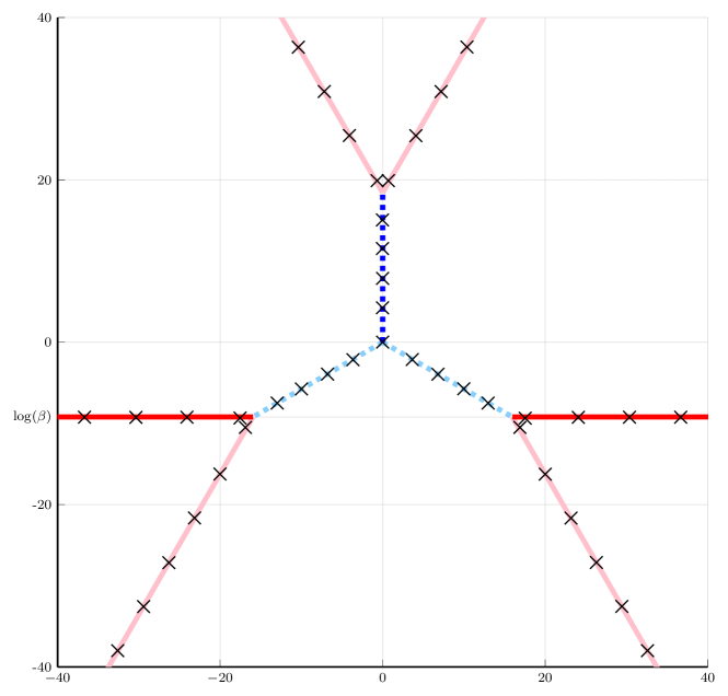
Figure 1. The zeros of $\Delta$ for $\beta=10^{-6}$. Also shown are line segments and rays along which the zeros lie, approximately.

It appears that they lie approximately along the dashed blue line segment and the solid red rays, and their lighter colored rotations about the origin by $2\pi/3$, $4\pi/3$. The rotational symmetry is immediately confirmed by the identity $\Delta(\alpha k)=\alpha^{2}\Delta(k)$, and implies that we only need to characterise the location of the solid red horizontal rays and dashed blue vertical line segment. To this end, consider $k$ with $\operatorname{Re}(k)\gg\lvert\operatorname{Im}(k)\rvert$, and observe that the dominant terms in $\Delta(k)$ are $\beta\alpha e^{-i\alpha k}$ and $\alpha^{2}e^{i\alpha^{2}k}$, while all other terms are $\mathcal{O}(1)$ in $\operatorname{Re}(k)$. Imposing that the leading order terms approximately cancel requires that $k_{n}\approx\left(2n-\frac{1}{3}\right)\pi+i\log(\beta)$ for $n\to\infty$. The existence of zeros close to $-\left(2n-\frac{1}{3}\right)\pi+i\log(\beta)$ is similarly justified. The zeros close to the dashed blue line segment arise when $\beta$ is very small so that, for $\lvert k\rvert$ not too large, the terms in $\Delta(k)$ with factor $\beta$ are negligible. Using the same kind of asymptotic argument as above, choosing a region of $\mathbb{C}$ such that two terms dominate the remaining one and requiring that those leading order terms cancel, we find that there is a finite number of zeros around $i\left(2n-1\right)\frac{\pi}{\sqrt{3}}$, for $n$ positive but not too large. Note that, although $0$ is a zero of $\Delta$, it is not the cube root of an eigenvalue, because no quadratic expression satisfies the boundary conditions.

The above arguments show that on the horizontal (red) rays,

(10) $$k_{n}=\kappa_{n}+i\log\beta+\epsilon_{n}, \qquad\mbox{where, as }|n|\to\infty,$$

$$\kappa_{n}=\pi\left(2n-\frac{\operatorname{sgn}(n)}{3}\right), \qquad\epsilon_{n}=\mathcal{O}\left(e^{-\sqrt{3}\pi\lvert n\rvert}\right).$$

The corresponding eigenfunctions are given by

(11) $$X_{n}=\sum_{j=0}^{2}e^{-i\alpha^{j}k_{n}x}(e^{-i\alpha^{j+1}k_{n}}-e^{-i\alpha^{j+2}k_{n}}).$$

It is not difficult to show that the adjoint operator has eigenvalues $k_{n}^{\star}=\overline{k_{n}}$ and eigenfunctions $X_{n}^{\star}$ given by the same formula as above for $X_{n}$ but with $k_{n}^{\star}$ replacing $k_{n}$.

General solution formula

We can express the solution of this boundary value problem as a generalised Fourier series, namely

(12) $$u(x,t)=\sum_{n}e^{-ik_{n}^{3}t}X_{n}(x)\frac{\langle u_{0},X_{n}^{\star}\rangle}{\langle X_{n},X_{n}^{\star}\rangle}.$$

We can now prove the following regularity result for the solution, which in particular confirms that no revival property can be supported by boundary value problems in this class.

Theorem 1.

Suppose $u_{0}\in\operatorname{L}^{2}(0,1)$. Then, for all $t>0$, the solution $u$ of the problem (5) with $0<\beta<1$ satisfies $u({}\cdot{},t)\in\operatorname{C}^{\infty}[0,1]$.

Proof.

Using the formula (11) for the eigenfunctions, we can compute

$$\left\langle X_{n},X_{n}^{\star}\right\rangle \hskip 40.00006pt=\sum_{j,r=0}^{2}\int_{0}^{1}e^{-i\alpha^{j}k_{n}x}\overline{e^{-i\alpha^{r}\overline{k_{n}}x}}dx\left(e^{-i\alpha^{j+1}k_{n}}-e^{-i\alpha^{j+2}k_{n}}\right)\overline{\left(e^{-i\alpha^{r+1}\overline{k_{n}}}-e^{-i\alpha^{r+2}\overline{k_{n}}}\right)}$$

$$=\sum_{j=0}^{2}\left(e^{-i\alpha^{j+1}k_{n}}-e^{-i\alpha^{j+2}k_{n}}\right)\left(e^{i\alpha^{j+2}k_{n}}-e^{i\alpha^{j+1}k_{n}}\right)$$

$$\hskip 10.00002pt+\sum_{\begin{subarray}{c}j,r=0:\\ \alpha^{j}\neq\alpha^{-r}\end{subarray}}^{2}\left[\frac{e^{-ik_{n}(\alpha^{j}-\alpha^{-r})}-1}{-ik_{n}(\alpha^{j}-\alpha^{-r})}\right]\left(e^{-i\alpha^{j+1}k_{n}}-e^{-i\alpha^{j+2}k_{n}}\right)\left(e^{i\alpha^{-(r+1)}k_{n}}-e^{i\alpha^{-(r+2)}k_{n}}\right).$$

Recalling expression (10) for the asymptotic behaviour of the eigenvalues, we find that the first sum, as $n\to\pm\infty$, is $e^{\sqrt{3}\lvert k_{n}\rvert}+\mathcal{O}(e^{\sqrt{3}\pi\lvert n\rvert})$.

The terms in the second sum each take one of the forms

$$\frac{e^{-ik_{n}(\alpha^{\ell}-\alpha^{m})}}{-ik_{n}(\alpha^{j}-\alpha^{-r})},\qquad\frac{e^{-ik_{n}(\alpha^{j}(1+\alpha^{\ell})-\alpha^{-r}(1+\alpha^{m}))}}{-ik_{n}(\alpha^{j}-\alpha^{-r})},$$

for $\ell,m\in\{0,1,2\}$ in the first form and $\ell,m\in\{1,2\}$ in the second form. Therefore, these terms are all dominated by the leading order term from the first sum. In summary, we obtain

$$\left\langle X_{n},X_{n}^{\star}\right\rangle=e^{\sqrt{3}\lvert k_{n}\rvert}+\mathcal{O}\left(\frac{e^{2\sqrt{3}\pi\lvert n\rvert}}{n}\right).$$

By Hölder’s inequality,

$$\langle u_{0},X_{n}^{\star}\rangle\leq\left\lVert u_{0}\right\rVert_{\operatorname{L}^{1}(0,1)}\left\lVert X_{n}^{\star}\right\rVert_{\operatorname{L}^{\infty}(0,1)}\lesssim\left\lVert u_{0}\right\rVert_{\operatorname{L}^{1}(0,1)}e^{\frac{\sqrt{3}}{2}\lvert\kappa_{n}\rvert},$$

with constant uniform in $n$. Therefore

$$\left\lVert\frac{\left\langle u_{0},X_{N}^{\star}\right\rangle}{\left\langle X_{n},X_{n}^{\star}\right\rangle}X_{n}\right\rVert_{\operatorname{L}^{\infty}(0,1)}$$

is bounded as $n\to\pm\infty$ and, for the $m$-th derivative, we obtain

$$\left\lVert\frac{\left\langle u_{0},X_{N}^{\star}\right\rangle}{\left\langle X_{n},X_{n}^{\star}\right\rangle}X_{n}^{(m)}\right\rVert_{\operatorname{L}^{\infty}(0,1)}=\mathcal{O}\left(n^{m}\right).$$

On the other hand, computing the imaginary part yields

$$\operatorname{Im}(k_{n}^{3}) =\operatorname{Im}\left(\kappa_{n}^{3}+3i\log(\beta)\kappa_{n}^{2}-3[\log(\beta)]^{2}\kappa_{n}-i[\log(\beta)]^{3}+\mathcal{O}\left(n^{2}e^{-\sqrt{3}\pi n}\right)\right)$$

$$=3i\log(\beta)\kappa_{n}^{2}+\mathcal{O}(1).$$

It follows that

$$e^{-ik_{n}^{3}t}=\mathcal{O}\left(e^{3\kappa_{n}^{2}t\log(\beta)}\right)$$

and, since $t\log(\beta)<0$ for $0<\beta<1$, this factor is decaying exponentially. Hence, for all $t>0$, the series in equation (12) for $u(x,t)$ converges absolutely uniformly in $x\in[0,1]$, and so do its term-by-term spatial derivatives. From the fact that $X_{n}\in\operatorname{C}^{\infty}[0,1]$, it follows that, for all $t>0$, $u({}\cdot{},t)\in\operatorname{C}^{\infty}[0,1]$. ∎

The case $\beta=0$

For this case, we know that the operator has infinitely many real eigenvalues, but that the eigenfunctions do not form a basis for the associated $\operatorname{L}^{2}$ space [22].

This boundary value problem was studied in [2], where the version of Proposition 1 for $\beta=0$ is proved. When the initial datum is in the domain of the operator, $u_{0}\in{\mathcal{D}_{0}}$, there exist a unique classical solution $u\in\operatorname{C}([0,\infty);H^{3}(0,1))\cap\operatorname{C}^{1}([0,\infty);\operatorname{L}^{2}(0,1))$ of the boundary value problem. When $u_{0}\in\operatorname{L}^{2}(0,1)$, there is a unique solution in the same class.

The estimates (7)-(9) with $\beta=0$ imply that the function

$$t\to\|u(\cdot,t)\|_{H^{1}(0,1)}$$

is in $\operatorname{L}^{2}(0,t)$, so that for almost all $t>0$, $u(\cdot,t)\in H^{1}(0,1)$ and the solution admits a weak first derivative. The heuristic argument presented after Proposition 1 points to the conclusion that there can be no fractalisation for any $u_{0}\in\operatorname{L}^{2}(0,1)$. Hence we arrive at the following conjecture.

Conjecture 1.

We conjecture that the revival property does not hold for the boundary value problem corresponding to $\beta=0$.

A proof of this conjecture might be possible by analysing the explicit structure of the explicit contour integral representation as derived by the unified transform method of Fokas [1, 6, 11, 12]. Using this transform, it can be shown that the boundary value problem corresponding to $\beta=0$, for a smooth $u_{0}$, has a unique solution $u(x,t)$, and that solution admits the explicit contour integral representation

$$u(x,t)=\frac{1}{2\pi}\int_{\mathbb{R}}{\rm e}^{ikx+ik^{3}t}\widehat{u_{0}}(k)dk\\ +\left\{\int_{\Gamma^{+}}{\rm e}^{ikx+ik^{3}t}\frac{\zeta^{+}(k)}{\Delta(k)}dk+\int_{\Gamma^{-}}{\rm e}^{ik(x-1)+ik^{3}t}\frac{\zeta^{-}(k)}{\Delta(k)}dk\right\}.$$

In this expression, $\Gamma^{\pm}$ are contours in ${\mathbb{C}}^{\pm}$, defined as the lines where the exponential ${\rm e}^{ik^{3}t}$ is purely oscillatory. The function $\widehat{u_{0}}(k)$ denotes the Fourier transform of $u_{0}$ on $[0,1]$, and $\zeta^{\pm}(k)$, $\Delta(k)$ are functions of $k$ only, fully determined by the initial datum $u_{0}$. The zeros of $\Delta$ are the cube roots of the eigenvalues of the spatial differential operator, and it can be shown that they are not on the integration contours. Hence the integrands in the last two integrals are analytic functions on the contours, and the integrals are well defined.

This integral representation is not equivalent to a discrete generalised Fourier series, and for $u_{0}\in\operatorname{L}^{2}(0,1)$ it would be necessary to prove its validity. While this goes beyond the scope of the present paper, we expect that the explicit asymptotic analysis of the integrand, in the spirit of the proof of Theorem 1, would yield a proof of the conjecture.

Remark 1.

The property of fractalisation does not imply the validity of revivals. Indeed, the quasi-periodic problem for the Airy equation mentioned above, with boundary conditions as in expression (2) and $\theta\notin\mathbb{Q}$, has solution with fractal dimension greater than 1 for all rational times, while the revival property does not seem to be supported for any other family of times. A more precise characterisation of the latter particular instance of fractalisation remains an interesting open problem.

The case $\beta=1$

In this case, we need to analyse the spectral structure of the operator

$$T_{1}=-i\partial_{x}^{3}:{\mathcal{D}_{1}}\longrightarrow\operatorname{L}^{2}(0,1).$$

It follows from general spectral theory that $A$ is self-adjoint, hence that $iA$ is the generator of a $C_{0}$ one-parameter semigroup. This guarantees, for any $u_{0}\in\operatorname{L}^{2}(0,1)$, the existence of a unique solution $u(x,t)\in\operatorname{C}([0,\infty);\operatorname{L}^{2}(0,1))$ of the associated boundary value problem (5).

If $u_{0}\in{\mathcal{D}_{1}}$, then $u$ is a strong solution: $u\in{\mathcal{D}_{1}}$ and

$$u\in C([0,\infty);H^{3}(0,1))\cap\operatorname{C}^{1}([0,\infty);\operatorname{L}^{2}(0,1)).$$

We are interested in the case when $u_{0}$ has some jumps discontinuities, but is otherwise smooth. While this is the case of most interest, the theorem below is proved in [3] for a more general class of initial data.

Theorem 2.

Assume that $u_{0}\in\operatorname{BV}[0,1]$ is real-valued, has singular part equal to zero and that it has only finitely many discontinuities. Assume in addition that $u_{0}$ satisfies a Hölder condition at $x=0$ and $x=1$.

Then, the solution of the boundary value problem (5), with $\beta=1$, admits the representation

$$u(x,t)=U_{\mathcal{R}}(x,t)+U_{\mathcal{C}}(x,t),\qquad x\in(0,1),\;t>0,$$

where

$U_{\mathcal{C}}({}\cdot{},t)\in\operatorname{C}(0,1)$ for all $t\in{\mathbb{R}}$, and

(13) $$U_{\mathcal{R}}(x,t)=\sum_{n=1}^{\infty}2\operatorname{Re}\left[\widehat{G_{u_{0}}}(n){\rm e}^{i(2n-\frac{1}{3})^{3}\pi^{3}t}{\rm e}^{i(2n-\frac{1}{3})\pi x}\right],$$

where

At any time of the form $t=\frac{p}{\pi^{2}q}$, with $p,q\in{\mathbb{N}}$ coprime, the function $U_{\mathcal{R}}(x,t)$ can be written as

(14) $$U_{\mathcal{R}}\left(x,\frac{p}{q\pi^{2}}\right)=\operatorname{Re}\left\{{\rm e}^{-i\frac{\pi}{27}\left(9x+\frac{p}{q}\right)}[L_{1}(x)+iL_{2}(x)-L_{3}]\right\},$$

where

$$L_{1}(x) =\sum_{k=0}^{q-1}d_{k}^{p,q}G_{u_{0}}\left(x+\frac{p}{3q}-\frac{k}{q}\right),$$

$$L_{2}(x) =\sum_{k=0}^{q-1}d_{k}^{p,q}[{\mathcal{H}}G_{u_{0}}]\left(x+\frac{p}{3q}-\frac{k}{q}\right),$$

$$L_{3} =\int_{0}^{1}G_{u_{0}}(y)\mathrm{d}y,$$

$\mathcal{H}$ denotes the $1$-periodic Hilbert transform, and

(15) $$d_{k}^{p,q}=\frac{1}{q}\sum_{m=0}^{q-1}{\rm e}^{2\pi i\left(mk+\left[4m^{3}-2m^{2}\right]p\right)/q}.$$

The conclusion of this theorem is that, up to a continuous perturbation, the solution of (5) with $\beta=1$ at rational times $t=\frac{p}{\pi^{2}q}$ is given by a finite superposition of copies of the initial datum and of the 1-periodic Hilbert transform of the initial datum. Since the periodic Hilbert transform maps every jump discontinuity to a logarithmic cusp, the profile of the solution at rational times, when the initial datum has jump discontinuities, is the superposition of a continuous function with a finite number of jumps and logarithmic cusps, namely it has the weak cusp revival property discussed in [3].

Numerical simulations

We used Julia to plot the solution, approximated by the truncated eigenfunction series. In the $\beta=1$ case, because the problem is selfadjoint, we used the ApproxFun package [20] to compute the eigenvalues and eigenfunctions directly and evaluate the inner products in the solution representation. When $0<\beta<1$, we instead calculate the $k_{n}$ as roots of $\Delta$, then use expression (11) for the eigenfunctions. For $k_{n}$ close to $0$, we use the Julia implementation [13] of the GRPF algorithm [15, 16], based on the argument principle and, for $\lvert k_{n}\rvert\gg 0$, we use the leading order asymptotic term in the expression for $k_{n}$ given in equation (10). We use the first 614 eigenvalues for the selfadjoint problem where $\beta=1$ and the first 120 for problems with $0<\beta<1$.

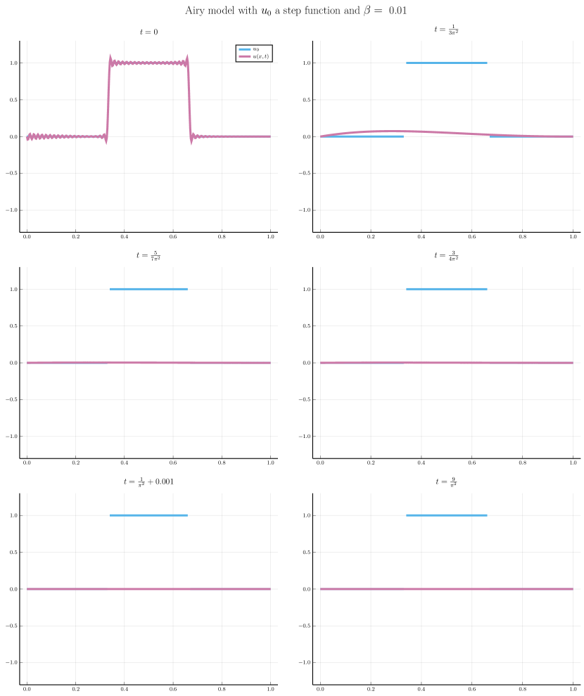
Figure 2.

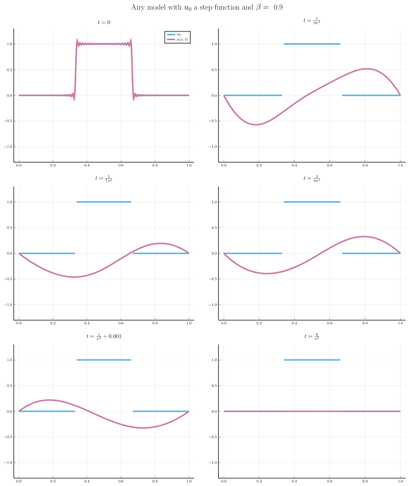
Figure 3.

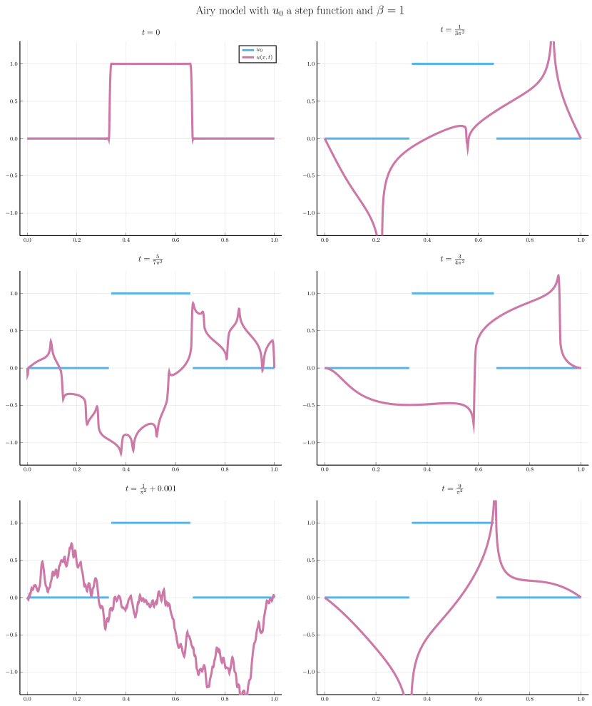
Figure 4.

We present plots of the solution starting from a piecewise constant initial datum for both cases. Specifically, in these plots the initial datum is the function

$$u_{0}(x)=\begin{cases}1&\frac{1}{3}<x<\frac{2}{3},\\ 0&\mbox{otherwise}.\end{cases}$$

The plots for $\beta=0.01$ and $\beta=0.9$ clearly show the solution starting from this discontinuous initial datum to be smooth (and decaying) at all positive times. The plots for $\beta=1$ show the cusps (which are infinite logarithmic cusps, though they are shown as finite by the graphic interface) generated by the discontinuities at rational times, and the fractalisation phenomenon at the generic time $\displaystyle{t=\frac{1}{\pi^{2}}+0.001}$.

References

- [1] S. A. Aitzhan, S. Bhandari, and D. A. Smith, Fokas diagonalization of piecewise constant coefficient linear differential operators on finite intervals and networks, Acta Appl. Math. 177 (2022), no. 2, 1–66.
- [2] Jerry L Bona, Shu Ming Sun, and Bing-Yu Zhang, A nonhomogeneous boundary-value problem for the Korteweg–de Vries equation posed on a finite domain, Communications in Partial Differential Equations 28 (2003), no. 7–8, 1391–1436.
- [3] L. Boulton, G Farmakis, B. Pelloni, and D.A. Smith, Jumps and cusps: Talbot effect in non-periodic dispersive pdes, preprint, 2024.
- [4] Lyonell Boulton, George Farmakis, and Beatrice Pelloni, Beyond periodic revivals for linear dispersive PDEs, Proceedings of the Royal Society A 477 (2021), no. 2251, 20210241.
- [5] Lyonell Boulton, Peter J. Olver, Beatrice Pelloni, and David A. Smith, New revival phenomena for linear integro–differential equations, Studies in Applied Mathematics 147 (2021), no. 4, 1209–1239.
- [6] Bernard Deconinck, Thomas Trogdon, and Vishal Vasan, The method of fokas for solving linear partial differential equations, SIAM Review 56 (2014), no. 1, 159–186.
- [7] N Dunford and J T Schwartz, Linear operators, part II spectral theory self adjoint operators in hilbert spaces, Wiley Interscience, 1963.
- [8] M Burak Erdoğan and Nikolaos Tzirakis, Dispersive partial differential equations. wellposedness and applications, vol. 86, London Mathematical Society Student Texts. Cambridge University Press, Cambridge, 2016.
- [9] G Farmakis, Revivals in time-evolution quasi-periodic problems, arXiv preprint, 2311.02780, 2023.
- [10] George Farmakis, Jing Kang, Peter J Olver, Changzheng Qu, and Zihan Yin, New revival phenomena for bidirectional dispersive hyperbolic equations, arXiv preprint arXiv:2309.14890.
- [11] AS Fokas and Beatrice Pelloni, A transform method for linear evolution pdes on a finite interval, IMA journal of applied mathematics 70 (2005), no. 4, 564–587.
- [12] AS Fokas and David A Smith, Evolution pdes and augmented eigenfunctions. finite interval, Advances in Differential Equations 21 (2016), no. 7/8, 735–766.
- [13] Forrest Gasdia, RootsAndPoles.jl: Global complex roots and poles finding in the Julia programming language, 2019.
- [14] Dunham Jackson, Expansion problems with irregular boundary conditions, Proceedings of the American Academy of Arts and Sciences 51.
- [15] Piotr Kowalczyk, Complex root finding algorithm based on delaunay triangulation, ACM Trans. Math. Softw. 41 (2015), no. 3.
- [16] by same author, Global complex roots and poles finding algorithm based on phase analysis for propagation and radiation problems, IEEE Transactions on Antennas and Propagation 66 (2018), no. 12, 7198–7205.
- [17] Kenneth DT-R McLaughlin and Nigel JE Pitt, On ringing effects near jump discontinuities for periodic solutions to dispersive partial differential equations, arXiv preprint arXiv:1107.1571 (2011).
- [18] Peter J Olver, Dispersive quantization, The American Mathematical Monthly 117 (2010), no. 7, 599–610.
- [19] Peter J Olver, Natalie E Sheils, and David A Smith, Revivals and fractalisation in the linear free space Schrödinger equation, Quarterly of Applied Mathematics 78 (2020), no. 2, 161–192.
- [20] Sheehan Olver and Alex Townsend, A practical framework for infinite-dimensional linear algebra, Proceedings of the 1st Workshop for High Performance Technical Computing in Dynamic Languages – HPTCDL ‘14, IEEE, 2014.
- [21] Beatrice Pelloni, The spectral representation of two-point boundary-value problems for third-order linear evolution partial differential equations, Proceedings of the Royal Society A: Mathematical, Physical and Engineering Sciences 461 (2005), no. 2061, 2965–2984.
- [22] Beatrice Pelloni and David A Smith, Spectral theory of some non-selfadjoint linear differential operators, Proceedings of the Royal Society A: Mathematical, Physical and Engineering Sciences 469 (2013), no. 2154, 20130019.
- [23] David A. Smith, Well-posed two-point initial-boundary value problems with arbitrary boundary conditions, 152 (2012), 473–496.
- [24] by same author, Well-posedness and conditioning of 3rd and higher order two-point initial-boundary value problems, arXiv:1212.5466, 2012.
- [25] by same author, Revivals and fractalization, Dynamical System Web (2020), 1–8.