Design Space Exploration for Particle Detector Read-out Implementations in Matlab and Simulink on the Example of the SHiP SBT

Abstract

On a very fundamental level, particle detectors share similar requirements for their read-out chain. This is reflected in the way that typical read-out solutions are developed, where a previous design is taken and modified to fit some changes in requirements. One of the two common approaches is the current-based read-out, where the waveform of the sensor output is sampled in order to later extract information from there. This approach is used in many detector applications using scintillation based detectors, including PET.
With this contribution, we will introduce how we use Matlab in order to simulate the read-out electronics of particle detectors. We developed this simulation approach as a base for our ongoing development of software-defined read-out ASICs that cover the requirements of a variety of particle detector types. Simulink was chosen as a base for our developments as it allows simulation of mixed-signal systems and comes with built-in toolkits to aid in developments of such systems.
With our approach, we want to take a new look at how we approach designing such a read-out, with a focus on digital signal processing close to the sensor, making use of known signal characteristics and modern methods of communications engineering. We are taking into account the time profile of an event, the bandwidth-limiting properties of the sensor and attached electronics, digitization stages and finally the parameterization of approaches for digital processing of the signal. We will show how we are applying the design approach to the development of a read-out for the proposed SHiP SBT detector, which is a scintillation based detector relying on SiPMs sensors, using this as an example for our modelling approach and show preliminary results.
Given the similarity in principle, the modelling approach could easily be modified for PET systems, allowing studies of the read-out chain to possibly gain in overall performance.

Data acquisition concepts; Digital Signal Processing (DSP); Front-end electronics for detector readout; Optical detector readout concepts; Simulation methods and programs; Software architectures (event data models, frameworks and databases) skip=5pt

1 Motivation

Fundamentally, particle detectors are not much different from each other. They deliver a current pulse that is the result of the detector response to the incident energy, folded with the electrical characteristics of the sensor and read-out electronics. In order to get a high-performance read-out, the complete system needs to be well understood. A common approach to develop an understanding of a complex system is to build a model of the system and test the model against real life observations. This approach is often taken in particle physics, using the power of modern computers to simulate the behavior of the whole detector and read-out system. In a detector chain, every domain has its own custom tooling for such modelling. The characteristics of an event in the individual channel are typically modelled with tools such as Geant4 [1], that simulate the particles’ behavior in the active material of the detector. The electrical characteristics of the sensor and peripheral electronics and their signal shaping effects are modelled using a derivative of SPICE, an established system for circuit simulations. The digital post-processing of such signals finally can be modelled with the tools we already use for digital design, e.g., Vivado or Cadence. All those tools are highly complex and reside within their own domain, only used by the experts that work on the particular subsystem. In order to derive requirements for our ASIC implementations, we want to be able to study the signals and signal processing of a system using a common tool chain. We have chosen Matlab/Simulink to implement a custom approach for studying the mixed-signal processing in particle detectors. In the following, we will provide a brief look into how we approach the modelling and how we are applying it to our developments for a real detector prototype.

2 Simulation of Particle Detector Read-Out in Matlab and Simulink

2.1 Overview

Matlab and Simulink are standard tools in engineering for simulation of complex control systems and mixed-signal systems, making it a reliable tool for our developments. In section 2.2 we will briefly describe how we separated the modelling domains and evaluate their implementations individually. The performance of the simulations will be then discussed in 2.4. In section 3.3 the Simulink model for the Search for Hidden Particles (SHiP) Surrounding Background Tagger (SBT) Detector will be discussed as a good example for both the modelling approach and performance and to show results achieved, which will be discussed in section 3.4.

2.2 Modelling Domains

Our approach requires modelling effort on multiple fronts. We have to model the input signal into the active part of the detector, which in this context is referred to as event modelling. Further, the response of the active part to incoming signal quanta has to be modelled, we call this the sensor modelling. The output of this sensor model is the detector signal current, that is processed by analog electronics, then digitized and further processed by digital signal processing means. Those we will refer to as analog and digital processing models.

Event and Sensor Modelling:

The input to the Simulink model is reflecting the time characteristics of the detector event. For the simulations performed in the context of this publication we have prepared results from Geant4 simulations, which can be loaded into Matlab, where we can add effects from the sensor, alike the dark counts of a Silicon Photo Multiplier (SiPM) in a Monte-Carlo fashion.

Simulink Transient Modelling:

Simulink is a tool that allows transient simulations of complex models [2]. It allows co-simulation of continuous and discrete time systems, making it a good match for simulating both the analog and the digital domain of the signal processing chain for a particle detector. Our models typically are made up of a continuous time part, that models the behavior of analog electronics and a discrete time system, that is an implementation of the digital domain logic in Matlab. Using the HDL Coder toolbox, we will be able to deploy our digital logic onto an FPGA for testing purposes [3].

Analog Modelling:

The analog domain of our model includes both the sensor response to in-coming particles and the analog signal processing, including pre-amplifiers and additional filtering that might be performed for signal shaping. In practice, the model complexity and accuracy can be chosen by the user, as the developed software does not rely on a specific model structure. As will be discussed later, we mainly resorted to using Laplace domain representation (system transfer functions) for expressing and solving the equations of the electrical systems. We took this approach, as it is a simple way of modelling continuous time signals and is well-supported in Simulink. Other possibilities would involve custom models or usage of the Simscape Electrical toolbox.

Digital Modelling:

We can either work with z-transform transfer functions or use any of the provided discrete time blocks from Simulink libraries for modeling the digital domain. This way we can simulate digital filters, perform mathematical operations on the signal or apply other kinds of transformations. Simulink supports multi-rate digital systems, allowing the user to take advantage of faster simulations by reducing the sample rate of subsystems by parallelization of data.

2.3 Simulation Control

Simulink models can be controlled by Matlab on a run to run basis, using Simulink.SimulationInput objects. With those, the parameters of a model can be set and inputs can be provided. The framework we developed for this purpose provides functions to automatically create simulation objects and arrange them in a way to allow fast simulations of large datasets.

2.4 Simulation Performance

For evaluation, we ran 10,000 simulations on an Intel NUC9i7QNX with a 6 Core i7-9750H and 64 GB RAM. In the context of this evaluation, we use the model we developed for simulation in the SHiP SBT application context. The model contains sub-models for the complete analog chain, a model of an on-FPGA SRAM for data buffering, including read and write logic and multiple feature extraction algorithms. Each simulation covers $1\text{\,}\mathrm{\SIUnitSymbolMicro s}$ of simulated detector signal and contains a single detector event. The time per simulation is shown in figure 3.

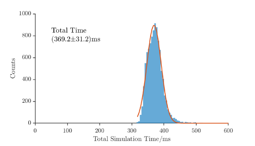
[t]0.49 [t]0.49

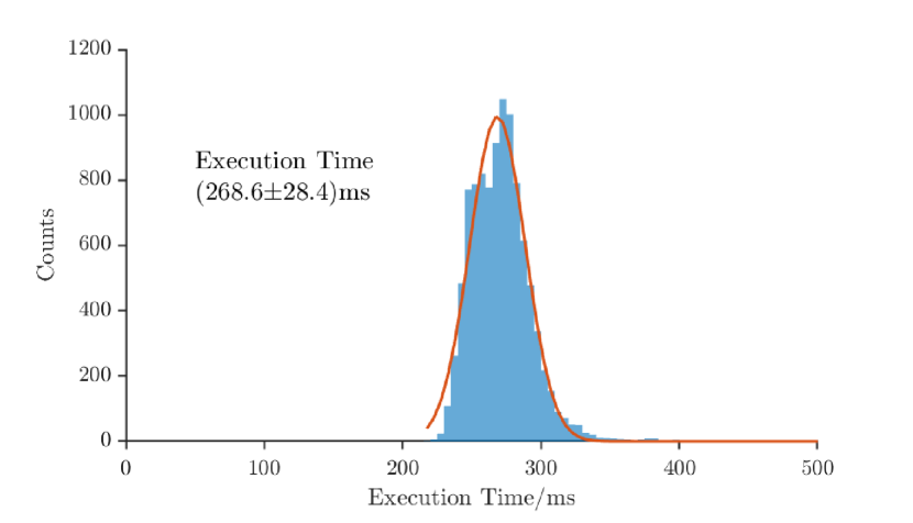
Figure 1: Total time per simulation, including simulation setup and teardown.

Figure 2: Time taken per simulation, without any pre- or post-processing functions.

Figure 3: Time performance of simulations using our software.

We utilize all cores for parallel simulation, making the overall run time even shorter. As can be seen from the displayed data, the average simulation takes about $380\text{\,}\mathrm{ms}$, including approximately $100\text{\,}\mathrm{ms}$ for model setup and tear down functions. The result shows only about $75\text{\,}\mathrm{\char 37\relax}$ time utilization for the actual simulation, making longer multi event, or more complex simulations an attractive option, in order to optimize for time performance.

3 Application to the SHiP SBT Detector

In order to demonstrate the accuracy and usefulness of the above introduced software, we choose to apply the approach to an ongoing detector development. We choose the SHiP SBT as a suitable application. The SHiP experiment is a particle physics experiment proposed for the ECN3 beam dump facility of the SPS at CERN [4, 5], where the SBT sub-detector serves as a background detector for the large vacuum decay vessel, that makes up the main part of the detector. [6].

3.1 SHiP SBT Detector Introduction

The detector features a long vacuum decay volume for possible hidden particles to decay with a longer baseline. To track possible intrusions into the decay volume, that could influence the measurements of the downstream detectors, the decay vessel is surrounded by the SHiP SBT, a scintillation detector, consisting of large steel tanks filled with a liquid scintillator. The individual steel tanks are equipped with Wavelength-shifting Optical Modules, which shift the light they absorb in wavelength and emit it into a light guide. The light guide is mounted to a PCB that hosts a ring of SiPMs, which read the light from the WOM tubes. The ring is made up from 40 individual Hamamtsu s14160-3050HS [7] silicon photomultipliers. For readout purposes, five SiPMs are connected in parallel to form a single read-out channel [5, 6]. The primary target of the SBT detector development is proof of interaction. Secondary targets are qualifying the deposited energy and a position resolution as high as possible. By combining the information of neighboring cells, hopefully the trajectory of a particle can be determined. The characteristics of photons measured by the SiPMs is largely dependent on the liquid scintillator used, the geometry, and reflectivity of the inner tank walls and photo conversion and collection probabilities of the WOM and SiPM.

3.2 SHiP SBT Event Model

Given the dependencies on tank geometry and scintillator properties, the simulation of the events is a task that is best left to specialized tools such as Geant4. For the purpose of this work, we are using the Geant4 model code that was written for the studies of a one-cell prototype detector [8]. It takes into account various detector characteristics, such as scintillation spectra and decay times of the liquid scintillator, wall reflectivity, absorption- and emission spectra of the wavelength shifting layer, the WOM transmission, and the wavelength dependent sensitivity of the SiPMs. We have performed Geant4 simulations, each containing a single event, with muons of different energies, ranging from $100\text{\,}\mathrm{MeV}$ to $10\text{\,}\mathrm{GeV}$ penetrating the detector box perpendicular to the large face at different positions. You can see the hit positions and box layout in figure 4. While we certainly not cover the whole range of possible events expected in operation of the SHiP SBT sub-detector, the data obtained this way will be suitable as an initial gauge for the usability and reliability of our software.

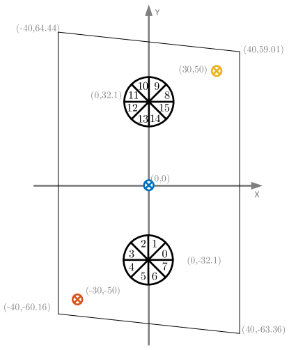
Figure 4: Sketched view of a SHiP SBT detector cell, with the WOM positions and SiPM groups indicated by the cake sliced circles, the numbers in the slices indicate the SiPM groups. The simulated beam positions are indicated by the crossed circles. All coordinates in centimeter, depiction not to scale.

From the Geant4 simulation data, we can derive some fundamental limits for the performance of the detector. As can be seen in figure 7, the arrival time of the first photon varies by approximately $0.7\text{\,}\mathrm{ns}$ on SiPM group 0. We observe a comparable fluctuation on all groups. Combining the groups yield a significantly better timing fluctuation of approximately $0.3\text{\,}\mathrm{ns}$. This sets the boundary for the achievable time resolution accordingly. Given the relatively high amount of dark counts present in SiPMs, triggering of the first photon is unlikely, and we will only be able to achieve a worse time resolution. For the photon number resolution, shown in figure 7, the photon number has a fluctuation of $\pm 20\text{\,}\mathrm{\char 37\relax}$, limiting the achievable photon number estimator resolution accordingly.

[t]0.49 [t]0.49

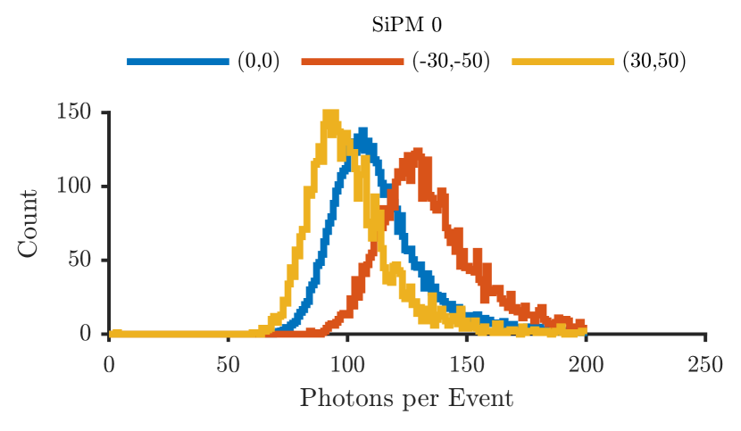
Figure 5: Arrival Time Distribution for the first photon of an event at SiPM Group 0. The individual distributions show a standard deviation on the arrival time of $0.7\text{\,}\mathrm{ns}$ with only a small deviation between the hit positions. The mean arrival time shows a strong dependence on the hit position, as can be expected.

Figure 6: Photon number distributions for photons collected on SiPM Group 0 per event. The individual distributions show a FWHM over mean of $40\text{\,}\mathrm{\char 37\relax}$. Also, we observe a distance dependent trend in the mean number of photons, while the total number of photons is roughly similar.

Figure 7: Time and photon number resolution for the SHiP SBT one cell prototype, derived from Geant4 simulations.

3.3 Simulink Model of a single Detector Channel

Using the output generated with Geant4, we can now use them as a basis for the simulations in our framework. We add dark counts to the simulated event photons in Matlab, with an adjustable dark count rate, the implementation is similar to [9]. In Simulink, we have to emulate the response of a SiPM to incoming photons. For this, we employ a modelling approach similar to [10] and [11], where the modelling of SiPMs in the context of the SHiP SBT has already been discussed. We use the equivalent circuit, as shown in figure 10. We add an idealized model of our front-end electronics to this, so we can account for the shaping effects of the coupling circuitry. The amplifier and coupling components are displayed in figure 10.

[c]0.60 [c]0.39

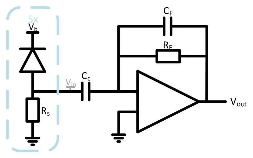
Figure 8: SiPM equivalent circuit model from [10].

Figure 9: SiPM connected to a trans-impedance front-end.

Figure 10: Equivalent circuitry as used for modelling purposes. For the SHiP SBT single channel model, we use five SiPM structures (highlighted in yellow) in parallel.

In figure 10, the distinction between firing and passive cells of a SiPM is made. For a SiPM with quenching impedance $R_{q}$ and $C_{q}$ and the cell capacity $C_{d}$, for $N$ total cells and $N_{f}$ fired cells, the fired cells contribute $R_{1}=\frac{R_{q}}{N_{f}}$, $C_{1}=C_{q}N_{f}$ and $C_{2}=C_{d}N_{f}$. The passive cells $R_{3}=\frac{R_{q}}{N-N_{f}}$, $C_{3}=C_{q}\left(N-N_{f}\right)$ and $C_{4}=C_{d}\left(N-N_{f}\right)$. In figure 10, we have added the coupling components $R_{s}$ and $C_{c}$ that we plan to add in the signal path. We simulate an ideal amplifier, with the frequency limiting pole provided by the feedback structure. The following equations were used to derive our models: I_d+s C_2 (V_1-V_3)+V1R1+s C_1 V_1&=0
s C_4 (V_2-V_3)+V2R3+s C_3 V_2=0
I_d+s C_2 (V_1-V_3)+s C_4 (V_2-V_3)-C_5 V_3=s+V3R6+s C_c V_3
Z_in= 1s Cc; Z_F= 11RF+s CF; ZFVinZin+ZF+ZinVoutZin+ZF=0; V_in=V_3 We can plug the solutions for $V_{3}$ and $V_{out}$ into a Simulink transfer function block and thus simulate the analog electronics. We performed a proxy verification by comparing the simulation results from Simulink to the SPICE model from [10] in figure 11.

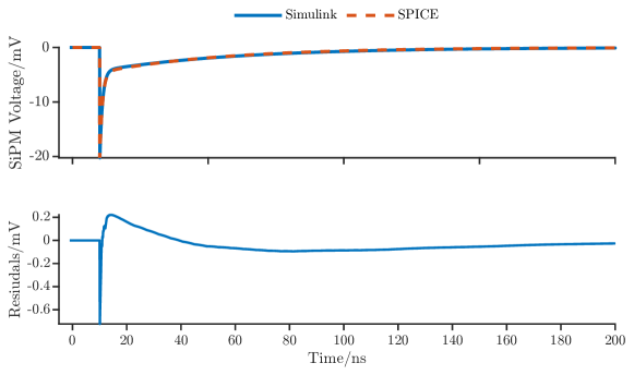
Figure 11: Comparison of SiPM signals captured with the SPICE model from [10] and our implementation in Simulink. Residuals are derived from a linear interpolation. The observed high residual at the leading edge of the Pulse is caused by the difference in step size between the signals.

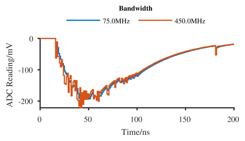
[t]0.465 [t]0.49

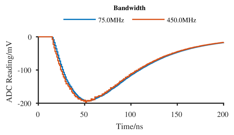
Figure 12: Example waveforms from simulations for different bandwidths.

Figure 13: Mean of waveforms for 100 runs vs. bandwidth.

Figure 14: Waveforms as obtained from our simulation model. In figure 14 we see, how higher bandwidths lead to the fast SiPM components becoming prominent and contributing large spikes to the signal, that could potentially reduce resolution. The slower base pulse, is the light curve of the liquid scintillator.

We can use Simulink to model various properties of an ADC, from basic parameters such as ADC bit resolution up to intrinsic non-linearities. The ADC output is then used to test different DSP methods on their performance. For the purpose of this paper, we tested a few basic approaches. The most common approach for timing and triggering, is to apply a threshold comparison to the signal, recording the time of threshold crossing as the signal timestamp. It is typically implemented using a fast comparator and a TDC. In this context, we simulate a digital threshold as a baseline algorithm for triggering and timing, as we plan to implement the read-out only using an ADC. As will be shown, an implementation with a fast comparator will not be beneficial. Parallel to that, we looked at a simple integration. Integration of the Signal Current is an estimator for the total charge created in a detector, and thus for the total deposited energy. Or in the case of the SHiP SBT the total number of photons collected. As a baseline, we will integrate the signal in the digital domain, by summing up all samples over threshold, which should yield a good estimator for the photon number. We also looked into sampling the peak of the signal, and we recorded the signals Time over Threshold (ToT), which can both serve as a photon number estimator, but also work as a good filter parameter for filtering noise triggers.

3.4 Simulation Results

We have looked into multiple parameter influences in order to narrow down the parameter space for a possible ASIC implementation. For each simulation run, we simulate a single model parameterization with $\mathrm{1}\mathrm{0}\mathrm{,}\mathrm{0}\mathrm{0}\mathrm{0}$ different events, taken from our Geant4 data sets. We have kept a trans-impedance of $500\text{\,}\mathrm{\SIUnitSymbolOhm}$ and an ADC dynamic range of -0.30.3, and fixed the SiPM parameters according to [10]. In total, we simulated 7.2 million detector events. For the initial simulations we have used the event data from the central hit position, see 4, and $1\text{\,}\mathrm{GeV}$ muons, reading data from SiPM group 0. We will later repeat simulations using different hit positions, energies and SiPMs in order to verify the initial simulations. To gain an overview of critical parameters, we performed a broad sweep of different combinations. From the simulated events, we obtained approximately 15.7 million total triggers from the electronics models. In order to reduce the unwanted triggers on noise or single photons, we looked at the distribution of the integral estimator, as can be seen in figure 17. The graph shows a histogram of the triggers obtained from simulation, for all cases in blue and for all noiseless simulations in yellow, showing a large pedestal of noise triggers with an integral smaller than $-5\text{\,}\mathrm{V}\times\mathrm{n}\mathrm{s}$.

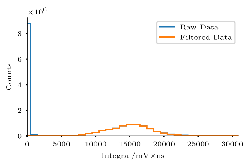
[t]0.465 [t]0.49

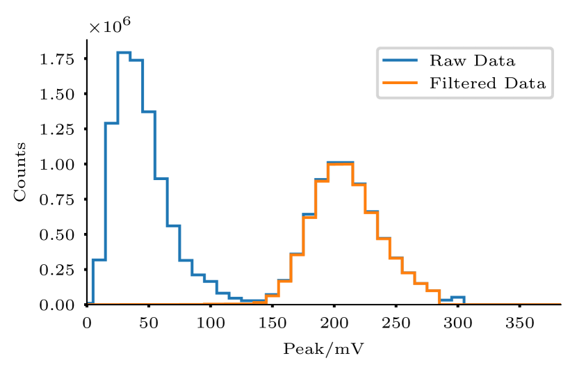
Figure 15: The distribution of the integral estimation.

Figure 16: The distribution of the peak estimator.

Figure 17: Distributions of the integral and peak estimators from our simulations. The low peak and integral regions are caused by noise triggers. A small, yet significant number of entries piled-up above $300\text{\,}\mathrm{mV}$ peak are caused by the limited dynamic range of the ADC, reaching saturation. High noise settings are the main cause for those entries.

In figure 17 you can see the distribution of signal peak estimations. As can be observed, the distribution is clipped at $300\text{\,}\mathrm{mV}$, which is the set input range limit that we set in simulation. The behavior was mainly caused by a high RMS noise setting, though also a small fraction of real events were affected. For a hardware implementation, we will need to choose a higher dynamic range to mitigate, or choose a lower trans-impedance. From the distributions of observed parameters, we choose some cut conditions to eliminate triggers that were likely caused by noise. For further analysis we only regarded data, where the integral estimation was larger than $5000\text{\,}\mathrm{m}\mathrm{V}\times\mathrm{n}\mathrm{s}$, the peak estimation was smaller-equal than $290\text{\,}\mathrm{mV}$ and the time-over-threshold was larger than $25\text{\,}\mathrm{ns}$. This left a dataset of 6.7 million triggers that we took into account for our analysis. For analysis, we extracted the parameterizations that formed the largest group along one parameter and fitted appropriate distribution functions to the histograms of the observables for each parameter step. We extracted the mean and standard deviation, as well as the uncertainty of the fit. A selection of our data is shown in figures 24 and 27. In figures 24 and 24 we show how the distribution width of the first timestamp is affected by the sampling rate and the front-end bandwidth. The influence of the ADC sample rate seems to be small, unfortunately the spread of the individual fit results is large, which can be expected, as the actual time binning with a sample rate of $1\text{\,}\mathrm{GHz}$ is limited to $1\text{\,}\mathrm{ns}$.
The influence of the front-end bandwidth, as shown in figure 24, shows the same issue especially for low bandwidths smaller than, $100\text{\,}\mathrm{MHz}$. As we expected, we observe a degradation of the time resolution with increasing bandwidth, as the influence of the high frequency components of the SiPM signals become more dominant than the slower underlying scintillator light curve. Parallel to that, figures 24 and 24, show the behavior of the relative integral resolution. The integral resolution overall seems to be less sensitive to changes in the sample rate and shows a small improvement with increased bandwidth. We have observed a negligible influence of the ADC bit resolution on both timestamp and integral resolution. In figures 24 and 24 the dependence on the trigger threshold is depicted. A clear dependence on the trigger threshold is obvious for both observables. In the timestamp domain, we see a jump below $25\text{\,}\mathrm{mV}$, which stems from the trigger now being sensitive to individual photons, with the single photon signal peaking at about $20\text{\,}\mathrm{mV}$, as shown in figure 11. We also observe two steps at approximately $-30\text{\,}\mathrm{mV}$ and $-60\text{\,}\mathrm{mV}$ that we can not fully explain yet. From the plots, we can conclude, that the trigger threshold should be chosen as low as possible. However, choosing a threshold to close to the single photon peak, would increase the amount of triggers, hence a compromise has to be made. More investigations, including the effect of a high dark-count rate, have to be performed here.

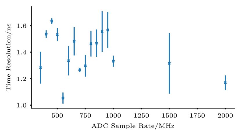
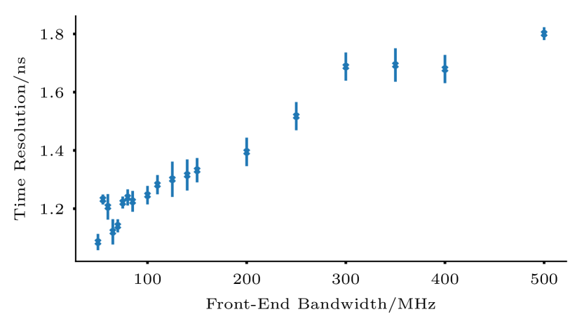
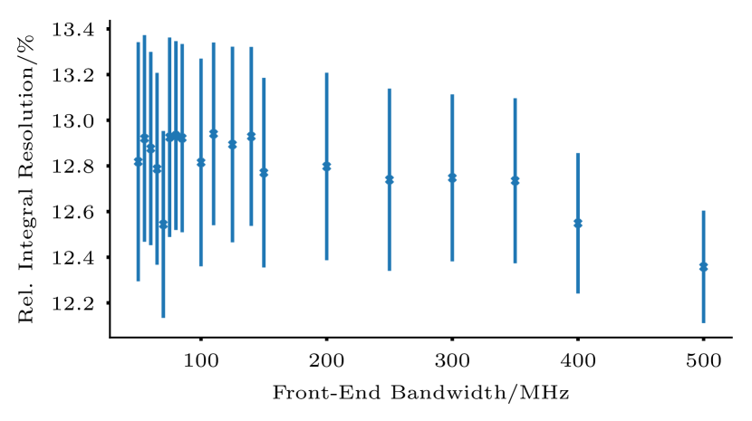
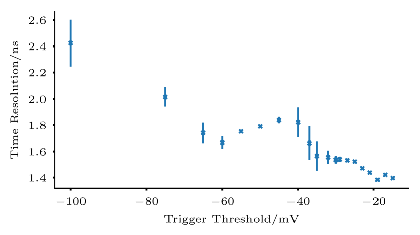
[c] [c]0.49 [c]0.49 [c] [c]0.49 [c]0.49 [c] [c]0.49 [c]0.49

Figure 18: Time resolution vs. sampling rate.

Figure 19: Integral resolution vs. sampling rate.

Parameterization: Bandwidth$=$ $150\text{\,}\mathrm{MHz}$; Trigger threshold $=$ $-30\text{\,}\mathrm{mV}$; ADC resolution $=$ $10\text{\,}\mathrm{b}\mathrm{i}\mathrm{t}$.

Figure 20: Time resolution vs. bandwidth.

Figure 21: Integral resolution vs. bandwidth.

Parameterization: Sample rate$=$ $1\text{\,}\mathrm{GHz}$; Trigger threshold $=$ $-30\text{\,}\mathrm{mV}$; ADC resolution $=$ $10\text{\,}\mathrm{b}\mathrm{i}\mathrm{t}$.

Figure 22: Time resolution vs. trigger threshold.

Figure 23: Integral resolution vs. trigger threshold.

Parameterization: Sample rate$=$ $400\text{\,}\mathrm{MHz}$; Bandwidth $=$ $150\text{\,}\mathrm{MHz}$; ADC resolution $=$ $10\text{\,}\mathrm{b}\mathrm{i}\mathrm{t}$.

Figure 24: Influence of different parameters on the estimated timestamp and integral, regarding only cases where no noise was present in the system. The error bars denote the variation introduced by the different parameterizations that were simulated. Only noiseless cases with no dark counts were regarded for the plots.

We also looked at the influence of RMS noise, as shown in figures 27 and 27. We used band-limited white noise by adding it to front-end output. Both time and integral resolution show the expected degradation of resolution with increasing noise, as can be seen in figure 27 and 27.

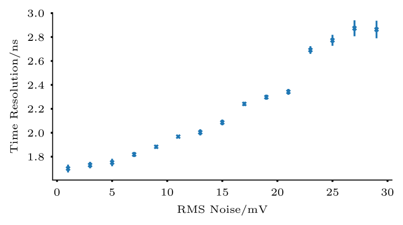
[c]0.49 [c]0.49

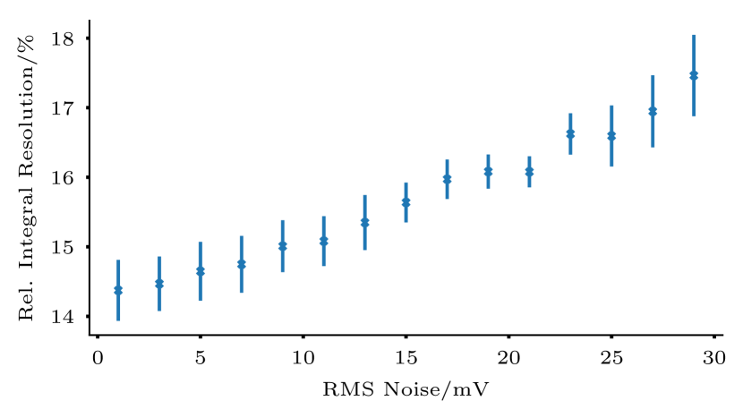
Figure 25: Time resolution vs. RMS Noise.

Figure 26: Integral resolution vs. RMS Noise.

Figure 27: Influence of the RMS noise on time and integral resolution, normalized by the applied trigger threshold.

4 Conclusion and Outlook

Our approach is capable of performing numerous simulations in a relatively short time frame, allowing to study a system across multiple parameters. We showed that we can produce sensible data, that can be used to make predictions for possible hardware implementations. In the future, we will use our software for the development of possible techniques and algorithms that could help with the improvement of the performance of the read-out for the SHiP SBT detector. Especially the time resolution, could potentially be improved using a suitable interpolation approach, similar to [12]. We plan to verify our simulations with live measurements on a SHiP SBT detector cell in 2024. Given our detector agnostic implementations, we can easily develop models for a PET detector and use the same software to perform design space explorations for a PET read-out system. We want to thank our collaborators from the SHiP Collaboration for the support of this work. Espacially we thank Andrii Kotenko and Vladyslav Orlov for important contributions to the Geant4 Model of the SBT detector cell.

References

- [1] S. Agostinelli, J. Allison, K. Amako, J. Apostolakis, H. Araujo, P. Arce et al., Geant4—a simulation toolkit, Nuclear Instruments and Methods in Physics Research Section A: Accelerators, Spectrometers, Detectors and Associated Equipment 506 (2003) 250.
- [2] The MathWorks Inc., “MATLAB Version: 9.12.0.2039608 (R2022a) Update 5.” The MathWorks Inc., 2022.
- [3] The MathWorks Inc., “HDL Coder Toolbox.” The MathWorks Inc., 2022.
- [4] W. Bonivento, A. Boyarsky, H. Dijkstra, U. Egede, M. Ferro-Luzzi, B. Goddard et al., Proposal to Search for Heavy Neutral Leptons at the SPS, Oct., 2013. 10.48550/arXiv.1310.1762.
- [5] C. Ahdida, A. Akmete, R. Albanese, J. Alt, A. Alexandrov, A. Anokhina et al., The SHiP experiment at the proposed CERN SPS Beam Dump Facility, The European Physical Journal C 82 (2022) 486.
- [6] J. Alt, M. Böhles, A. Brignoli, A. Conaboy, P. Deucher, C. Eckardt et al., Performance of a First Full-Size WOM-Based Liquid Scintillator Detector Cell as Prototype for the SHiP Surrounding Background Tagger, Nov., 2023.
- [7] Hamamatsu Photonics, MPPC S14160-3050HS Silicon Photo Multiplier, June, 2020.
- [8] F. Lyons, “GitHub - fairlyons/ship_wom_testbeam at 4cells.”
- [9] J. Pulko, F. R. Schneider, A. Velroyen, D. Renker and S. I. Ziegler, A Monte-Carlo model of a SiPM coupled to a scintillating crystal, Journal of Instrumentation 7 (2012) P02009.
- [10] J. Grieshaber, Calculation and Simulation of Silicon Photomultiplier Signals, bachelor Thesis, Albert-Ludwigs-Universität Freiburg, Freiburg, Feb., 2022.
- [11] F. Villa, Y. Zou, A. Dalla Mora, A. Tosi and F. Zappa, SPICE Electrical Models and Simulations of Silicon Photomultipliers, IEEE Transactions on Nuclear Science 62 (2015) 1950.
- [12] L. Jokhovets, A. Erven, C. Grewing, M. Herzkamp, P. Kulessa, H. Ohm et al., Improved Rise Approximation Method for Pulse Arrival Timing, IEEE Transactions on Nuclear Science 66 (2019) 1942.