Optimal sampling for stochastic and natural gradient descent

Abstract

We consider the problem of optimising the expected value of a loss functional over a nonlinear model class of functions, assuming that we have only access to realisations of the gradient of the loss. This is a classical task in statistics, machine learning and physics-informed machine learning. A straightforward solution is to replace the exact objective with a Monte Carlo estimate before employing standard first-order methods like gradient descent, which yields the classical stochastic gradient descent method. But replacing the true objective with an estimate ensues a “generalisation error”. Rigorous bounds for this error typically require strong compactness and Lipschitz continuity assumptions while providing a very slow decay with sample size. We propose a different optimisation strategy relying on a natural gradient descent in which the true gradient is approximated in local linearisations of the model class via (quasi-)projections based on optimal sampling methods. Under classical assumptions on the loss and the nonlinear model class, we prove that this scheme converges almost surely monotonically to a stationary point of the true objective and we provide convergence rates.

Keywords  natural gradient, optimisation on manifolds, active learning, weighted least-squares method, optimal sampling, importance sampling, risk minimisation, convergence rates

AMS subject classifications   49M15, 93E24, 68T07, 90C30, 60H30

1 Introduction

Let $\mathcal{X}$ be a set equipped with a probability measure $\rho$ and $\mathcal{H}:=\mathcal{H}(\mathcal{X},\rho)$ be a Hilbert space of functions defined on $\mathcal{X}$, equipped with the norm $\|\cdot\|$. Given a loss function $\ell:\mathcal{H}\times\mathcal{X}\to\mathbb{R}$, we consider the optimisation problem

$$\min_{v\in\mathcal{M}}\mathcal{L}(v),\qquad\mathcal{L}(v):=\int\ell(v;x)\,\mathrm{d}\rho(x)=\mathbb{E}_{x\sim\rho}[\ell(v;x)]$$ (1)

where $\mathcal{M}\subseteq\mathcal{H}$ is a possibly nonlinear model class and $\mathcal{L}$ is the risk or expected loss. When computing the integral is infeasible, a common approach is to replace the exact risk with an empirical risk (that is, a Monte Carlo estimate of the risk) before employing a standard optimisation scheme. However, using an estimated risk instead of the true risk can result in a “generalisation error”. Rigorous bounds for this error usually require compactness of $\mathcal{M}$ and Lipschitz continuity of $\mathcal{L}$ and provide a very slow decay with increasing sample size [12]. This slow decay is unfavourable in settings where high accuracy is required, or sample generation (or acquisition) is costly. Moreover, a plain sampling from $\rho$ can lead to a bad condition number of the resulting empirical risk [11] and consequently introduces numerical instabilities in optimisation algorithms.

1.1 Methodology and motivation

To address these issues, we propose a new iterative algorithm that performs successive corrections in local linearisations of $\mathcal{M}$. To be specific, we define a filtered probability space $(\Omega,\Sigma,\mathbb{P},(\mathcal{F}_{t})_{t\geq 0})$, with $\mathcal{F}_{t}$ depending on the iterates up to step $t$, and assume that at every step $t\in\mathbb{N}$, there exists an $\mathcal{F}_{t}$-measurable linear space $\mathcal{T}_{t}$ of dimension $d_{t}$ that approximates $\mathcal{M}$ locally around the current iterate $u_{t}$. Typically, for a parametrised model class $\mathcal{M}=\{F(\theta):\theta\in\mathbb{R}^{d}\}$, where $F:\mathbb{R}^{d}\to\mathcal{H}$ is differentiable, the space $\mathcal{T}_{t}$ around $u_{t}=F(\theta_{t})$ can be taken as the linear span of functions $\partial_{k}F(\theta_{t})$, $k=1,\ldots,d$, or a subset of these functions. If $\mathcal{L}$ admits a Fréchet derivative at $u_{t}$, we can define the gradient $\nabla\mathcal{L}(u_{t}):=g_{t}\in\mathcal{H}$ as the Riesz representative of the Fréchet derivative. Then, we can introduce an estimator $P_{t}^{n}$ of the $\mathcal{H}$-orthogonal projector $P_{t}\colon\mathcal{H}\to\mathcal{T}_{t}$, using evaluations of functions at points $x^{t}_{1},\ldots,x^{t}_{n}$, and perform a linear update $\bar{u}_{t+1}:=u_{t}-s_{t}P_{t}^{n}g_{t}$ with step size $s_{t}$ in the direction of the approximate projection of the negative gradient $-P_{t}^{n}g_{t}$. This yields the intermediate iterate $\bar{u}_{t+1}$. Since the $\bar{u}_{t+1}$ is not guaranteed to lie in the original model class $\mathcal{M}$, we perform a retraction (or recompression) step $u_{t+1}:=R_{t}(\bar{u}_{t+1})$, where $R_{t}:\mathcal{H}\to\mathcal{M}$ is an $\mathcal{F}_{t}$-measurable map that pushes $\bar{u}_{t+1}$ back to the model class $\mathcal{M}$ with a controllable error in the risk $\mathcal{L}$. The proposed algorithm can thus be presented as

$$\bar{u}_{t+1} :=u_{t}-s_{t}P_{t}^{n}g_{t},\qquad g_{t}:=\nabla\mathcal{L}(u_{t}),$$ (2)

$$u_{t+1} :=R_{t}(\bar{u}_{t+1}),$$

whereas we refer to Figure 1 for a graphical illustration. To control the variance of the iterates, we propose to estimate the orthogonal projection $P_{t}$ using optimal sampling methods, generalising the approach from [11]. The algorithm can be seen as a natural gradient descent (NGD) on manifold, using an empirical estimate of the orthogonal projection. With the projection $P_{t}^{n}g_{t}$ defined in terms of point evaluations of the gradient $g_{t}(x^{t}_{1}),\ldots,g_{t}(x^{t}_{n})$, the resulting algorithm can also be interpreted as a variant of stochastic gradient descent (SGD), using a batch of $n$ samples at each step.

Figure 1: Illustration of the proposed algorithm: based on an iterate $u_{t}\in\mathcal{M}$ and the choice of a linear space $\mathcal{T}_{t}$, an approximation $P_{t}^{n}g_{t}\in\mathcal{T}_{t}$ of the true gradient $g_{t}$ is first obtained via a random operator $P_{t}^{n}$. Then an update $\bar{u}_{t+1}=u_{t}-s_{t}P_{t}^{n}g_{t}$ is obtained given a step size $s_{t}$. Then, the next iterate $u_{t+1}\in\mathcal{M}$ is obtained through application of the retraction map $R_{t}$.

Performing a retraction with a projected gradient is a standard procedure in iterative methods with nonlinear model classes. However, since empirical (quasi-)projections have been thoroughly investigated, estimating the operator $P_{t}$ instead of the risk $\mathcal{L}$ allows for a refined analysis and improved convergence rates. The proposed first-order optimisation scheme can achieve the theoretically best approximation rates for deterministic gradient descent with retraction.

1.2 Contributions

We analyse the convergence of algorithm (2) to a minimiser or stationary point of the true risk $\mathcal{L}$ (not an empirical estimate) over the model class $\mathcal{M}$, possibly yielding theoretical bounds for the generalisation error. To provide qualitative theoretical guarantees for convergence, we do not consider line search methods for adaptive step size selection and assume that the step size $s_{t}$ is $\mathcal{F}_{t}$-measurable. We reason that a stable algorithmwould require a line search method with certified error bounds, which in turn requires estimating the risk $\mathcal{L}$ with guaranteed accuracy. This would command an a priori variance bound, which seems an implausible assumption in practice.

Our approach contrasts with many classical SGD approaches in two ways.

1. We define the risk as a functional on a (potentially infinite-dimensional) Hilbert space $\mathcal{H}$ and ensure that the descent direction is close to the gradient of $\mathcal{L}$ in $\mathcal{H}$. This allows us to consider the optimisation not over a parameter space but the corresponding model class of functions $\mathcal{M}=\{F(\theta):\theta\in\mathbb{R}^{d}\}$. This brings the advantage that Lipschitz smoothness and (strong) convexity parameters of the function $\mathcal{L}$ are often known exactly while, at the same time, being prohibitively large or inaccessible for the combined parameter-to-risk map $\theta\mapsto\mathcal{L}(F(\theta))$. Direct access to the smoothness and convexity parameters also means that the hyper-parameters (like step size) are easy to choose, and parameter tuning should not be required.

2. We assume that we have control over the sample generation process and adopt the viewpoint of active learning. An optimal sampling procedure ensures that the gradient is estimated with minimal and bounded variance. This results, in general, in a faster and more monotone convergence, as illustrated in Figure 7 in section 6.

The presentation in equation (2) provides a general framework for analysing stochastic gradient descent-type algorithms such as SGD and NGD. In particular, we provide (to the best of our knowledge) the first proof of convergence for NGD in this general setting. The convergence rates of our algorithms in different settings are presented in Table 1.

To do this, we consider a general class of estimates $P_{t}^{n}$ of the orthogonal projection $P_{t}$. Particular instances encompass least squares projections and quasi-projections, and we discuss the relevance of optimal sampling to reduce their variance. We show that under certain assumptions on the risk $\mathcal{L}$ and the sequences of operators $P_{t}^{n}$, step sizes $s_{t}$ and retractions $R_{t}$, the resulting optimisation scheme converges almost surely to a stationary point of the true risk.

We prove convergence of the proposed algorithm under the standard $L$-Lipschitz-smoothness ($L$-smoothness) and $\lambda$-Polyak–Łojasiewicz ($\lambda$-PL) assumptions. In particular, Theorem 4.3 provides non-asymptotic convergence bounds in expectation when both $L$-smoothness and $\lambda$-PL are satisfied. Almost sure asymptotic convergence is demonstrated in Theorem 4.11 under $L$-smoothness and in Corollaries 4.13 and 4.16 under a strong form of the $\lambda$-PL assumption. An overview of the corresponding convergence rates is provided in Table 1. Finally, we consider the convergence under the general $\lambda$-PL condition in Theorem 4.19.

		rates
assumptions		GD	best-case (ours)	worst-case (ours)	SGD
(B) + (LS) + (CR)		$\mathcal{O}(t^{-1})$ [10, 8]	$\mathcal{O}(t^{-1+\varepsilon})$ [eq. (35)]	$\mathcal{O}(t^{-1/2+\varepsilon})$ [eq. (36)]	$\mathcal{O}(t^{-1/2+\varepsilon})$ [34]
(LS) + (SPL) + (CR)		$\mathcal{O}(a^{t})$ [10, 8]	$\mathcal{O}(a^{t})$ [eq. (39)]	$\mathcal{O}(t^{1-2\varepsilon})$ [eq. (45)]	$\mathcal{O}(t^{1-2\varepsilon})$ [34]

Table 1: Almost sure convergence rates for different algorithms with $\varepsilon\in(0,\tfrac{1}{2})$ and $a\in(0,1)$ depending on the chosen step size. The required assumptions can be found in the linked references and equations.

1.3 Related work

The analysis of SGD algorithms in the case $\mathcal{M}=\mathcal{H}=\mathbb{R}^{d},d\in\mathbb{N}$, relies classically on the ABC condition,

$$\mathbb{E}\left[\|\widehat{\nabla\mathcal{L}(u)}\|^{2}\right]\leq A(\mathcal{L}(u)-\mathcal{L}_{\mathrm{min}})+B\|\nabla\mathcal{L}(u)\|^{2}+C,$$

where $\widehat{\nabla\mathcal{L}(u)}$ is an unbiased estimate of the gradient $\nabla\mathcal{L}(u)$ and $\mathcal{L}_{\mathrm{min}}$ is the infimum of $\mathcal{L}$ on $\mathcal{H}$. This condition is presented in [30] as “the weakest assumption” for analysing SGD in the non-convex setting. The parameter $C$ in the ABC condition captures the variance of the stochastic gradient and critically influences the convergence rate. In the best case ($C=0$), the resulting algorithm exhibits the same convergence rate as classical gradient descent (GD). In the typical case ($C>0$), however, the algorithm follows the classical SGD rates. Our work can be seen as a refined analysis of SGD, focusing on the constants $B$ and $C$ of the ABC condition.

In the preceding section, we have discussed how two adaptations of the classical SGD scheme are particularly relevant to guarantee convergence with a uniform rate:

1. working in the ambient function space $\mathcal{H}$ and using a controlled empirical (quasi-)projection ensures that the descent direction is close to an $\mathcal{H}$-orthogonal projection of the gradient of $\mathcal{L}$ in $\mathcal{H}$,

2. an optimal sampling procedure ensures that the gradient’s projection is estimated with bounded and close to minimal variance for a given sampling budget.

When expressed in the parameter space for a nonlinear model class, the optimisation scheme (2) can be seen as a Newton-like algorithm, which is known in the machine learning community as natural gradient descent (NGD) [37, 40, 38, 6]. The idea of choosing problem-adapted samples is well-known as importance sampling and has been explored for learning neural networks [9, 1, 2]. However, in general, there is no efficient importance sampling strategy for estimating a risk functional simultaneously for all functions from a highly nonlinear set $\mathcal{M}$ (see, e.g., the negative results for low-rank tensor networks in [20]). For this reason, we adopt an adaptive approach using successive updates in linear spaces, for which optimal sampling distributions have been rediscovered recently [11] and can be computed explicitly.

Recent years have seen a lot of active developments in the field of optimal weighted least squares projections [11, 15]. Using the least squares projection $P_{t}^{n}$ as an estimate of $P_{t}$ allows (up to possible conditioned sampling) to satisfy a quasi-optimality property in expectation [24], i.e. for all $v\in\mathcal{H},$

$$\mathbb{E}\left[{\|v-{P}^{n}_{t}v\|^{2}}\right] \leq\left(1+c\tfrac{d_{t}}{n}\right){\|v-P_{t}v\|^{2}}$$ (3)

for some constant $c$. When $P_{t}^{n}$ is a quasi-projection instead of a least-squares projection, we obtain for any $v\in\mathcal{H}$ an unbiased estimation $P_{t}^{n}v$ of the orthogonal projection $P_{t}v$. As a consequence of Lemma B.2, this estimator satisfies

$$\mathbb{E}\left[\|v-P_{t}^{n}v\|^{2}\right]\leq(1+\tfrac{d_{t}}{n})\|v-P_{t}v\|^{2}+\tfrac{d_{t}-1}{n}\|P_{t}v\|^{2}.$$ (4)

In particular, the quasi-projection does not guarantee quasi-optimality. The reader might thus be surprised that a quasi-projection yields comparable results to an optimally weighted least squares projection, when the latter clearly seems superior to the former. The flaw in this argument lies in comparing only a single step of the algorithm. Corollary 4.9 shows that both procedures perform similarly when multiple steps are taken. Using a least squares projection based on volume-rescaled sampling [14, 39] presents both advantages, i.e. the corresponding empirical projection is unbiased and achieves quasi-optimality in expectation.

Our work is on the same line as the two recent works [1, 2], where the practical relevance of optimal sampling in machine learning is demonstrated. Our theoretical results indicate that it is beneficial to extend the works mentioned above to cure some theoretical illnesses in learning with neural networks:

1. Both works linearise the network only in the last layer, resulting in samples that are optimal only for updating this last layer. However, changes in earlier layers are even more significant since the following part of the network amplifies errors in these layers.

2. Both works use a random sample for the orthogonalisation step. This was already proposed in [15], where it was also discussed that the worst-case bounds for the number of samples needed for a stable orthogonalisation may be infeasible. This may arguably happen for a model class as complicated as neural networks.

3. The samples are not drawn according to the optimal distribution but are subsampled from a larger i.i.d. sample from $\rho$. The approximation with respect to this subsample can thus not be better than the approximation using the full sample.

We finally touch on the topic of step size selection for first-order optimisation methods with stochastic descent directions. A naïve, constant choice of step sizes can already lead to oscillations around the local minima in the deterministic setting. This problem is only exacerbated by a non-vanishing variance of the gradient estimator. Although adaptive step size selection strategies, such as exact or backtracking line search, can circumvent this issue in the deterministic case, they can not be applied straightforwardly in the stochastic setting. Different stochastic step size selection methods have been proposed in the literature, some of which we list below.

• Trust region methods for functions with noisy function and gradient evaluation are investigated in [43]. Assuming $\mathcal{H}=\mathbb{R}^{d}$ and the error of the function estimates $\hat{\mathcal{L}}(u_{t})$ and gradient estimate $\hat{g}_{t}$ are almost surely uniformly bounded by $\varepsilon>0$, it is shown in [43] that the iterates accumulate in critical sets and that iterates of gradients $\{\|\hat{g}_{t}\|\leq\mathcal{O}(\varepsilon+\sqrt{\varepsilon})\}$. This generalises the fact that critical points are accumulation points of gradient descent and is similar in spirit to our discussion in Remark 4.2.

• Step sizes that are defined based on the history of previous gradient estimates are commonly used in machine learning (cf. the concept of gradient diversity in [48]). For the application of AdaGrad in $\mathcal{H}=\mathbb{R}^{d}$ it is shown in [33], that such a strategy results in the convergence rate $\mathbb{E}[\min_{t=1,\ldots,T}\|g_{t}\|^{1-2\varepsilon}]\in\mathcal{O}(T^{-1/4+\varepsilon})$ for $\varepsilon\in(0,\tfrac{1}{2})$ for certain non-convex objectives $\mathcal{L}$.

• Extensions of the classical Polyak step size rule to the stochastic setting have been considered e.g. in [36].

• A classical approach is to choose a deterministic step size sequence satisfying the Robbins–Monro condition a priori.

1.4 Outline

The remainder of this work is organised as follows. Section 2 introduces different estimators of the orthogonal projection and provides bias and variance bounds that are necessary for our analysis. The assumptions for our propositions are summarised and discussed in section 3. We state our convergence theory in section 4, where section 4.1 covers convergence in expectation and section 4.2 covers almost sure convergence. The topic of step size selection is briefly discussed in section 5. Finally, section 6 discusses the assumptions and illustrates the theoretical results for linear problems on bounded and unbounded domains in section 6.1 and 6.2, respectively, and for shallow neural networks in section 6.3. These examples also vindicate the expense that comes with optimal sampling and empirical (quasi-)projections.

2 Estimators of orthogonal projections

This section is devoted to the explicit construction of estimators $P_{t}^{n}$ of the $\mathcal{H}$-orthogonal projection $P_{t}\colon\mathcal{H}\to\mathcal{T}_{t}$ onto a given space $\mathcal{T}_{t}$ at step $t$ of our algorithm. These estimators use $n$ samples $x^{t}_{1},\ldots,x^{t}_{n}$, drawn from a suitable distribution on $\mathcal{X}$ that depends on $\mathcal{T}_{t}$ and are independent from the $\sigma$-algebra $\mathcal{F}_{t}$, generated by the samples $\{(x^{\tau}_{1},\ldots,x^{\tau}_{n}):1\leq\tau<t\}$ and $u_{0}$. The iterate $u_{t}$ is $\mathcal{F}_{t}$-measurable and therefore $g_{t}$ is also $\mathcal{F}_{t}$-measurable by the Doob –Dynkin lemma. We also assume that the space $\mathcal{T}_{t}$ is $\mathcal{F}_{t}$-measurable, as is the case when $\mathcal{T}_{t}$ is a linearization of $\mathcal{M}$ at $u_{t}$.

In what follows, we restrict ourselves to a Hilbert space $\mathcal{H}=\mathcal{H}(\mathcal{X},\rho)$ equipped with the scalar product

$$(u,v)=\int(L_{x}u)^{\intercal}(L_{x}v)\,\mathrm{d}{\rho(x)},$$ (5)

for a suitable family of linear operators $\{L_{x}:\mathcal{H}\to\mathbb{R}^{l}\}_{x\in\mathcal{X}}$, $l\in\mathbb{N}$. Two prominent examples of this setting are the following.

1. The Lebesgue space $L^{2}(\mathcal{X},\rho)$ corresponds to the Hilbert space $\mathcal{H}$ with the choice $L_{x}v:=v(x)$.

2. The Sobolev space $H^{1}(\mathcal{X},\rho)$ corresponds to the Hilbert space $\mathcal{H}$ with the choice $L_{x}v:=\begin{pmatrix}v(x)\\ \nabla v(x)\end{pmatrix}$.

The first example is a classical $L^{2}$ regression setting, while the second example is a natural setting for the solution of a class of partial differential equations using physics-informed learning. Given an orthonormal basis $\{b_{k}\}_{k=1}^{d_{t}}$ of $\mathcal{T}_{t}$, the projection $P_{t}g_{t}$ of $g_{t}\in\mathcal{H}$ onto the subspace $\mathcal{T}_{t}$ can be written as

$$P_{t}g_{t}=\sum_{k=1}^{d_{t}}\eta_{k}b_{k}\qquad\text{with}\qquad\eta_{k}:=(g_{t},b_{k}).$$ (6)

We now introduce four different estimators $\hat{P}_{t}^{n}$ of $P_{t}$, that correspond to different estimators of $\eta_{k}$ for $k=1,\ldots,d_{t}$. They all satisfy bias and variance bounds of the form

$$\mathbb{E}\left[(g_{t},P_{t}^{n}g_{t})\,\big{|}\,\mathcal{F}_{t}\right] \geq c_{\mathrm{bias},1}\|P_{t}g_{t}\|^{2}-c_{\mathrm{bias},2}\|P_{t}g_{t}\|\|(I-P_{t})g_{t}\|$$ (7)

$$\mathbb{E}\left[\|P_{t}^{n}g_{t}\|^{2}\,\big{|}\,\mathcal{F}_{t}\right] \leq c_{\mathrm{var},1}\|P_{t}g_{t}\|^{2}+c_{\mathrm{var},2}\|(I-P_{t})g_{t}\|^{2},$$

with non-negative constants $c_{\mathrm{bias},1/2}$ and $c_{\mathrm{var},1/2}$ and where the conditional expectation is taken over the samples $x^{t}_{1},\ldots,x^{t}_{n}$.

2.1 Non-projection

In the following, we consider a fixed step $t\in\mathbb{N}$ and define $\operatorname{supp}(\mathcal{T}_{t}):=\bigcup_{v\in\mathcal{T}_{t}}\operatorname{supp}(\|L_{\raisebox{0.0pt}{\,$\bullet$}\,}v\|)$. To estimate the integral in (5), we introduce a sampling measure $\mu_{t}$ and weight function $w_{t}$ such that

$$w_{t}\,\mathrm{d}{\mu_{t}}=\,\mathrm{d}{\rho}\qquad\text{on}\qquad\operatorname{supp}(\mathcal{T}_{t}).$$ (8)

An unbiased estimate of the inner product $(u,v)$ can then be defined as

$$(u,v)_{n}:=\frac{1}{n}\sum_{i=1}^{n}w_{t}(x_{i})(L_{x_{i}}u)^{\intercal}(L_{x_{i}}v),$$

where the $x_{1},\ldots,x_{n}$ are i.i.d. samples from $\mu_{t}$.

Assume that $\mathcal{B}_{t}:=\{\varphi_{k}\}_{k=1}^{d}$ with $d\geq d_{t}$ forms a generating system of $\mathcal{T}_{t}$. Then an approximation of $g\in\mathcal{H}$ with respect to the system $\mathcal{B}_{t}$ is given by

$$P_{t}^{n}g:=\sum_{k=1}^{d}\hat{\zeta}_{k}\varphi_{k}\qquad\text{with}\qquad\hat{\zeta}_{k}:=(g,\varphi_{k})_{n}.$$ (9)

It is easy to see that $P_{t}^{n}$ is not a projection. Moreover, when $\mathcal{B}_{t}$ is not an orthonormal basis, this is not an unbiased estimate of the orthogonal projection $\bm{P_{t}}$. It is nevertheless important to study this operator because its use in (2) yields the standard SGD method when $\mathcal{H}=L^{2}(\mathcal{X},\rho)$ and $\ell(v;x)=\tilde{\ell}(v(x);x)$ with $\tilde{\ell}(\cdot;x):\mathbb{R}\to\mathbb{R}$ satisfies certain regularity assumptions. To see this, recall that SGD approximates $\mathcal{L}(v)$ by

$$\mathcal{L}_{n}(v):=\frac{1}{n}\sum_{i=1}^{n}\ell(v;x_{i})=\frac{1}{n}\sum_{i=1}^{n}\tilde{\ell}(v(x_{i});x_{i}),$$

where the $x_{i}$ are samples from $\rho$, and $w_{t}=1$. Now assume that $\mathcal{M}=\{F(\theta):\theta\in\mathbb{R}^{d}\}$ with a differentiable parametrisation map $F:\mathbb{R}^{d}\to\mathcal{H}$. Denoting by $\theta_{t}\in\mathbb{R}^{d}$ the parameter’s value of $u_{t}=F(\theta_{t})$, we can define $\varphi_{k}=\partial_{k}F(\theta_{t})$ and $\mathcal{T}_{t}:=\operatorname{span}\{\varphi_{k}:1\leq k\leq d\}$. SGD then uses the chain rule $D_{\theta}\mathcal{L}_{n}(F(\theta))=D_{v}\mathcal{L}_{n}(F(\theta))\circ D_{\theta}F(\theta)$ to compute the gradient

$$(\nabla_{\theta}\mathcal{L}_{n}(F(\theta)),e_{k})=\langle D_{v}\mathcal{L}_{n}(F(\theta)),\langle D_{\theta}v(\theta),e_{k}\rangle\rangle=\langle D_{v}\mathcal{L}_{n}(F(\theta)),\varphi_{k}\rangle.$$

Recall that the Fréchet derivative of $\mathcal{L}_{n}$ in $\mathcal{H}=L^{2}(\mathcal{X},\rho)$ is given by

$$\langle D_{v}\mathcal{L}_{n}(v),\varphi_{k}\rangle=\frac{1}{n}\sum_{i=1}^{n}\tilde{\ell}^{\prime}(v(x_{i});x_{i})\varphi_{k}(x_{i})=(\tilde{\ell}^{\prime}(v(\raisebox{0.0pt}{\,$\bullet$}\,);\raisebox{0.0pt}{\,$\bullet$}\,),\varphi_{k})_{n}.$$

On the other hand, by Leibniz’s integral rule (Proposition A.1), it holds for sufficiently regular loss functions that $\nabla_{v}\mathcal{L}(v)=\tilde{\ell}^{\prime}(v(\raisebox{0.0pt}{\,$\bullet$}\,);\raisebox{0.0pt}{\,$\bullet$}\,)$. Hence, if the loss is sufficiently regular and $\mathcal{H}=L^{2}(\mathcal{X},\rho)$, we can write the gradient of SGD as

$$(\nabla_{\theta}\mathcal{L}_{n}(F(\theta)),e_{k})=(\nabla_{v}\mathcal{L}(F(\theta)),\varphi_{k})_{n}=\hat{\zeta}_{k},\qquad\text{i.e.}\qquad\hat{\zeta}=\nabla_{\theta}\mathcal{L}_{n}(F(\theta)).$$ (10)

The following lemma bounds the bias and variance of $P_{t}^{n}$, and its proof can be found in appendix B.

Lemma 2.1.

Assume that $x_{1},\ldots,x_{n}$ are i.i.d. samples from $\mu_{t}$ given $\mathcal{F}_{t}$. Let $G\in\mathbb{R}^{d\times d}$ such that $G_{kl}:=(\varphi_{k},\varphi_{l})$ and let $\lambda_{*}(G)$ and $\lambda^{*}(G)$ denote the smallest positive and the largest eigenvalue of $G$, respectively. Moreover, let $\mathfrak{K}_{t}(x):=\lambda^{*}\left(\sum_{k=1}^{d_{t}}(L_{x}b_{k})(L_{x}b_{k})^{\intercal}\right)$ and $k_{t}:=\|w_{t}\mathfrak{K}_{t}\|_{L^{\infty}(\rho)}$. Then, the operator $P_{t}^{n}$ defined in equation (9) satisfies (7) with constants

$$c_{\mathrm{bias},1}=\lambda_{*}(G),\qquad c_{\mathrm{bias},2}=0,\qquad c_{\mathrm{var},1}=\tfrac{\lambda^{*}(G)^{2}(n-1)+\lambda^{*}(G)k_{t}}{n}\qquad\text{and}\qquad c_{\mathrm{var},2}=\tfrac{\lambda^{*}(G)k_{t}}{n}.$$

These bounds are tight.

2.2 Quasi-projection

From Lemma 2.1, it is clear that the system $\mathcal{B}_{t}$ has to be chosen meticulously in order for the bias and variance terms to remain bounded. This is addressed in the present section, where $\mathcal{B}_{t}$ is chosen as an orthonormal basis, entirely removing the dependence on the condition number of the Gramian matrix, which is equal to identity.

Consider a fixed step $t\in\mathbb{N}$ and assume that $\mathcal{B}_{t}:=\{b_{k}\}_{k=1}^{d_{t}}$ forms an $\mathcal{H}$-orthonormal basis of $\mathcal{T}_{t}$. Hence $G_{kl}:=(b_{k},b_{l})=\delta_{kl}$. Then the quasi-projection of $g\in\mathcal{H}$ with respect to the basis $\mathcal{B}_{t}$ is given by

$$P_{t}^{n}g:=\sum_{k=1}^{d_{t}}\hat{\eta}_{k}b_{k}\qquad\text{with}\qquad\hat{\eta}_{k}:=(g,b_{k})_{n}.$$ (11)

Although this is still not a projection, it is an unbiased estimate of the real projection $P_{t}$, defined in (6). The relevance of this operator stems from its connection to natural gradient descent. Suppose that $\mathcal{M}=\{v=F(\theta):\theta\in\mathbb{R}^{d}\}$ and $\mathcal{T}_{t}:=\operatorname{span}\{\varphi_{k}:1\leq k\leq d\}$ with $\varphi_{k}:=\partial_{k}F(\theta)$. Define the Gramian matrix $H_{kl}:=(\varphi_{k},\varphi_{l})$ and suppose that $b=H^{+}\varphi$ is an orthonormal basis for $\mathcal{T}_{t}$. Then, we can write

$$\eta=H^{+}\zeta\quad\text{with}\quad\zeta_{k}=(g,\varphi_{k})\quad\qquad\text{and}\qquad\quad\hat{\eta}=H^{+}\hat{\zeta}\quad\text{with}\quad\hat{\zeta}_{k}=(g,\varphi_{k})_{n}.$$ (12)

The quasi-projection’s coefficients $\hat{\eta}$ are hence an estimate of the orthogonal projection’s coefficients $\eta$, where $\zeta$ is replaced by the Monte Carlo estimate $\hat{\zeta}$. This demonstrates that the algorithm presented in equation (2) can be seen as a natural gradient descent, as defined in [40].

Even though $P_{t}^{n}g$ technically depends on the choice of basis $\mathcal{B}_{t}$, this dependence is irrelevant in the subsequent analysis. Indeed, for every valid choice of $\mathcal{B}_{t}$ the following estimate holds.

Lemma 2.2.

Assume that $x_{1},\ldots,x_{n}$ are i.i.d. samples from $\mu_{t}$ given $\mathcal{F}_{t}$. Let $\mathfrak{K}_{t}(x):=\lambda^{*}\left(\sum_{k=1}^{d_{t}}(L_{x}b_{k})(L_{x}b_{k})^{\intercal}\right)$ and $k_{t}:=\|w_{t}\mathfrak{K}_{t}\|_{L^{\infty}(\rho)}$. Then the operator $P_{t}^{n}$ defined in equation (11) satisfies (7) with constants

$$c_{\mathrm{bias},1}=1,\qquad c_{\mathrm{bias},2}=0,\qquad c_{\mathrm{var},1}=\tfrac{n-1+k_{t}}{n}\qquad\text{and}\qquad c_{\mathrm{var},2}=\tfrac{k_{t}}{n}.$$

These bounds are tight.

Proof.

Follows from Lemma 2.1, since $G=I$. ∎

Although the dependence on $G$ is removed by the specific choice of an orthonormal basis, the bias and variance bounds still depend on $k_{t}$. This constant depends on the space $\mathcal{T}_{t}$ and may be unbounded. Consider, for example, a space $\mathcal{T}_{t}$ of univariate polynomials with degree $d_{t}-1$ in $\mathcal{H}=L^{2}(\rho)$. Then, we have the following two bounds:

1. $k_{t}=d_{t}^{2}$, if $w_{t}\equiv 1$ and $\rho$ is the uniform measure on $\mathcal{X}:=[-1,1]$,

2. $k_{t}=\infty$, if $w_{t}\equiv 1$ and $\rho$ is the standard Gaussian measure on $\mathcal{X}:=\mathbb{R}$.

This demonstrates that it is crucial to control $k_{t}$ during the optimisation, which requires choosing a suitable sampling measure $\mu_{t}$ or corresponding weight function $w_{t}$. Theorem 3.1 in [45] shows that the weight function $w_{t}$ that minimises $k_{t}:=\|w_{t}\mathfrak{K}_{t}\|_{L^{\infty}(\rho)}$ is given by

$$w_{t}=\|\mathfrak{K}_{t}\|_{L^{1}(\rho)}\mathfrak{K}_{t}^{-1}.$$

The subsequent lemma provides a formula for $\mathfrak{K}_{t}$ and the easier-to-compute surrogate $\tilde{\mathfrak{K}}_{t}^{-1}$. Both choices, $w_{t}=\|\mathfrak{K}_{t}\|_{L^{1}(\rho)}\mathfrak{K}_{t}^{-1}$ and $w_{t}=\|\tilde{\mathfrak{K}}_{t}\|_{L^{1}(\rho)}\tilde{\mathfrak{K}}_{t}^{-1}$, guarantee $k_{t}\leq d_{t}$ and coincide when $l=1$. The corresponding sampling is referred to as generalised Christoffel sampling.

Lemma 2.3.

Let $\{b_{k}\}_{k=1}^{d_{t}}$ be an $\mathcal{H}$-orthonormal basis for the $d_{t}$-dimensional subspace $\mathcal{T}_{t}\subseteq\mathcal{H}$. Recall that

$$\mathfrak{K}_{t}(x):=\lambda^{*}\left(\sum_{k=1}^{d_{t}}(L_{x}b_{k})(L_{x}b_{k})^{\intercal}\right)$$

and denote by

$$\mathfrak{K}_{\mathcal{T}_{t}}(x):=\sup_{v\in\mathcal{T}_{t}}\frac{\|L_{x}v\|_{2}^{2}}{\|v\|}$$

the generalised inverse Christoffel function (or variation function, cf. [45]). It holds $\mathfrak{K}_{t}=\mathfrak{K}_{\mathcal{T}_{t}}$. Moreover, define

$$\tilde{\mathfrak{K}}_{t}(x):=\operatorname{trace}\left(\sum_{k=1}^{d_{t}}(L_{x}b_{k})(L_{x}b_{k})^{\intercal}\right)=\sum_{k=1}^{d_{t}}\|L_{x}b_{k}\|_{2}^{2}.$$

It holds $\mathfrak{K}_{t}\leq\tilde{\mathfrak{K}}_{t}$, with equality if $l=1$ in (5). Moreover, it holds that $\|\tilde{\mathfrak{K}}_{t}\|_{L^{1}(\rho)}=\int\tilde{\mathfrak{K}}_{t}\,\mathrm{d}{\rho}=d_{t}$.

A proof of this lemma can be found in appendix C.

Remark 2.4.

(Gradient dependent important sampling) Lemma B.2, which is used to prove Lemma 2.2, provides the even tighter variance bound

$$\frac{1}{n}\int w_{t}(x)\mathfrak{K}_{t}(x)\|L_{x}g\|_{2}^{2}\,\mathrm{d}{\rho(x)}\leq\tfrac{1}{n}\|w_{t}\mathfrak{K}_{t}\|_{L^{\infty}(\rho)}\|g\|^{2}=\tfrac{k_{t}}{n}\|g\|^{2}.$$ (13)

Choosing the weight function $w_{t}$ to minimise the upper bound $k_{t}=\|w_{t}\mathfrak{K}_{t}\|_{L^{\infty}(\rho)}$ instead of the left-hand side in (13) is thus not optimal and ignores the relation of $w_{t}$ to the current gradient $g$. A notable example follows from the bound

$$\frac{1}{n}\int w_{t}(x)\mathfrak{K}_{t}(x)\|L_{x}g\|_{2}^{2}\,\mathrm{d}{\rho(x)}\leq\frac{1}{n}\int\mathfrak{K}_{t}(x)\,\mathrm{d}{\rho(x)}\sup_{x\in\mathcal{X}}w(x)\|L_{x}g\|_{2}^{2}=\frac{k_{t}}{n}\sup_{x\in\mathcal{X}}w_{t}(x)\|L_{x}g\|_{2}^{2}.$$

If we can explicitly bound $\|L_{x}g\|_{2}^{2}$, we can adapt the weight function to the current gradient. For instance, if the model class is compact and $\|L_{x}g\|_{2}\leq C\|g\|$ is uniformly bounded for all $x\in\mathcal{X}$ and all gradients $g$, the right-hand side is also uniformly bounded, and the bias remains bounded during optimisation. This shows that stochastic gradient descent can converge even without optimal sampling, as commonly performed in practice.

Remark 2.5.

Depending on the model class, sampling from the associated optimal sampling measure $\mu_{t}$ at step $t$ can be a nontrivial problem since $\mathfrak{K}_{t}$ (or $\tilde{\mathfrak{K}}_{t}$) can be non-smooth and extremely multimodal. For linear spaces with advantageous structure, however, sampling can rely on existing results [11, 15, 4, 18, 3]. Also, for tree tensor networks, the optimal sampling density admits a representation as a tree tensor network, and marginalisation can be performed with efficient tensor algebra, which allows for an efficient sequential sampling [25, Appendix]. For general model classes, the optimal sampling density can be approximated by covering arguments [45].

2.3 Least squares projection

The preceding section shows that a quasi-projection with optimal sampling yields an estimator with bounded bias and variance constants. However, it is not a projection, which is desirable to guarantee stability. For this reason, we now consider a weighted least squares projection based on the generalised Christoffel sampling introduced in the previous section. This projection is based on i.i.d. samples and is a slight modification of the quasi-projection. We define the empirical Gramian $\hat{G}_{kl}:=(b_{k},b_{l})_{n}$ as well as $\hat{\eta}_{k}:=(g,b_{k})_{n}$. Then the least squares projection of $g\in\mathcal{H}$ onto $\mathcal{T}_{t}$ is given by

$$P_{t}^{n}g:=\sum_{k=1}^{d}\hat{\vphantom{\rule{1.0pt}{6.14584pt}}\smash{\hat{\eta}}}_{k}b_{k}\qquad\text{with}\qquad\hat{\vphantom{\rule{1.0pt}{6.14584pt}}\smash{\hat{\eta}}}:=\hat{G}^{+}\hat{\eta}.$$ (14)

Note that since $P_{t}^{n}$ is indeed a projection, it does not depend on the specific choice of basis $\mathcal{B}_{t}$. In particular, the computation of the projection no longer requires knowledge of an orthonormal basis. However, this comes at the cost that $\bm{P_{t}^{n}}$ is not an unbiased estimate of $\bm{P_{t}}$. At this point, we want to point out the similarity of this estimate to the quasi-projection in (12). In contrast to the quasi-projection’s coefficients $\hat{\eta}$, not only $\zeta$ is replaced by the Monte Carlo estimate $\hat{\zeta}$, but the Gramian $G$ is estimated as well. This provides a different interpretation of equation (2) as a natural gradient descent, as defined in [40].

Although replacing the exact Gramian with an estimate may ensue an error, the size of this error is of the same order as the error that is ensued by replacing $\zeta$ by $\hat{\zeta}$. Moreover, if an orthonormal basis is used (i.e. $G=I$) and if the samples are drawn optimally, it can be shown [11] that

$$\mathbb{P}\left[\|I-\hat{G}\|\leq\delta\right]\leq 2d_{t}\exp(-\tfrac{\delta^{2}n}{2d_{t}}).$$

In this case, the estimated Gramian is close to the true Gramian with high probability, and quasi-projection and projection do not differ significantly. Since the quantity $\|I-\hat{G}\|$ essentially controls the quality of the estimate, it is reasonable to draw the sample points not from $\mu_{t}$ but to add an additional conditioning step that ensures stability, i.e. to condition the sample points on the event

$$\mathcal{S}_{\delta}:=\{\|I-\hat{G}\|\leq\delta\}.$$ (15)

This also allows the use of subsampling methods to reduce the number of samples further  [24, 16, 5].

Remark 2.6.

Note that although an orthonormal basis is no longer required to compute the least squares projection, it is still required in all currently known methods to compute an exact sample from $\mu_{t}$. This is a known problem and the focus of current research.

Lemma 2.7.

Let $\delta\in(0,1)$ and $x_{1},\ldots,x_{n}\sim\mu_{t}$ be i.i.d. samples from $\mu_{t}$ given $\mathcal{F}_{t}$ and conditioned to satisfy the event $\mathcal{S}_{\delta}$, with $\mathbb{P}(\mathcal{S}_{\delta}\,|\,\mathcal{F}_{t})=p_{\mathcal{S}_{\delta}}>0$. Let $\mathfrak{K}_{t}(x):=\lambda^{*}\left(\sum_{k=1}^{d_{t}}(L_{x}b_{k})(L_{x}b_{k})^{\intercal}\right)$ and $k_{t}:=\|w_{t}\mathfrak{K}_{t}\|_{L^{\infty}(\rho)}$. Then, the operator $P_{t}^{n}$ defined in equation (14) satisfies (7) with bias and variance constants

$$c_{\mathrm{bias},1}=1,\qquad c_{\mathrm{bias},2}=\tfrac{\sqrt{k_{t}}}{(1-\delta)\sqrt{p_{\mathcal{S}_{\delta}}n}},\qquad c_{\mathrm{var},1}=\tfrac{1}{(1-\delta)^{2}p_{\mathcal{S}_{\delta}}}\tfrac{n-1+k_{t}}{n}\qquad\text{and}\qquad c_{\mathrm{var},2}=\tfrac{1}{(1-\delta)^{2}p_{\mathcal{S}_{\delta}}}\tfrac{k_{t}}{n}.$$

The proof of this lemma can be found in appendix D.

Remark 2.8.

Note that both the projection and quasi-projection require knowledge of an orthonormal basis. If this basis is not known a priori, a single step of either the projection or quasi-projection requires ${O}(d_{t}^{3})$ operations and is significantly more expensive than a simple SGD step, which requires ${O}(d_{t})$ operations. This difference is aggravated by the cost of the optimal sampling scheme compared to the generation of samples from the reference measure $\rho$. However, Lemma 2.1 implies that the convergence rate of SGD depends on the condition number of the Gramian matrix $\kappa(G)$ and on $k_{t}$, which may both grow uncontrollably during optimisation. We accept this tradeoff of more expensive steps in favour of controlling these two constants and, thereby, the convergence rate in the true risk $\mathcal{L}$.

2.4 Least squares projection with determinantal point process and volume sampling

Despite all the advantages that the least squares projection brings, it also suffers from a severe disadvantage, namely that $c_{\mathrm{bias},2}>0$, which makes the estimate not well-suited for iterative procedures, as will be discussed in Remark 4.2. When $\mathcal{H}=L^{2}(\rho)$, this problem is solved by a weighted least squares projection $P_{t}^{n}$ based on volume-rescaled sampling [14]. As before, let $\{b_{k}\}_{k=1}^{d_{t}}$ be an $L^{2}(\rho)$-orthonormal basis of $\mathcal{T}_{t}$ and denote by $b(x)=(b_{j}(x))_{j=1}^{d_{t}}\in\mathbb{R}^{d_{t}}$ the vector of all basis functions. Let $\mu_{t}=w_{t}^{-1}\rho$ be the optimal measure for the i.i.d. setting, with $w_{t}(x)^{-1}=\frac{1}{d_{t}}\|b(x)\|_{2}^{2}$. Given a set of points $\bm{x}:=(x_{1},\ldots,x_{n})\in\mathcal{X}^{n}$, we consider the weighted least-squares projection associated with the empirical inner product

$$(u,v)_{n}=\frac{1}{n}\sum_{i=1}^{n}w_{t}(x_{i})u(x_{i})v(x_{i}).$$

The points $\bm{x}:=(x_{1},\ldots,x_{n})$ are drawn from the volume-rescaled distribution $\gamma_{n}^{\mu_{t}}$ defined by

$$\,\mathrm{d}{\gamma_{n}^{\mu_{t}}(\bm{x})}=\frac{n^{d_{t}}(n-d_{t})!}{n!}\det(\hat{G}(\bm{x}))\,\mathrm{d}{\mu_{t}^{\otimes n}(\bm{x})},$$

where $\hat{G}(\bm{x})$ is the empirical Gramian matrix $\hat{G}(\bm{x})_{k,l}=(b_{k},b_{l})_{n}$ and $\mu_{t}^{\otimes n}$ denotes the product measure on $\mathcal{X}^{n}$. This distribution tends to favour a high likelihood with respect to the optimal sampling measure $\mu_{t}^{\otimes n}$ in the i.i.d. setting and a high value of the determinant of the empirical Gramian matrix. For $n=d_{t}$, $\gamma_{d_{t}}^{\mu_{t}}$ corresponds to a projection determinantal point process (DPP) with distribution

$$\,\mathrm{d}{\gamma_{d_{t}}(\bm{x})}=\frac{1}{d_{t}!}\det(B(\bm{x})^{T}B(\bm{x}))\,\mathrm{d}{\rho^{\otimes d_{t}}(\bm{x})}$$

with $B(\bm{x})_{i,j}=b_{j}(x_{i})$. Whenever two selected features $b(x_{i})$ and $b(x_{k})$ are equal for $i\neq k$, the matrix $B(\bm{x})$ becomes singular and the density of $\gamma_{d_{t}}$ vanishes. This introduces a repulsion between the points. For $n>d_{t}$, a sample from $\gamma_{d_{t}}^{\mu_{t}}$ is composed (up to a random permutation) by $d_{t}$ points $x_{1},\ldots,x_{d_{t}}$ drawn from the DPP distribution $\gamma_{d_{t}}$, and $n-d_{t}$ i.i.d. points $x_{d_{t}+1},\ldots x_{n}$ drawn from the measure $\mu_{t}$ (see [14, Theorem 2.7] or [39, Theorem 4.7]).

Given a sample from $\gamma^{\mu_{t}}_{n}$, we have the remarkable result that the least-squares projection $P_{t}^{n}$ is an unbiased estimate of $P_{t}$ (see [14, Theorem 3.1] and [39, Theorem 4.13]) and that we have a control on the variance [39, Theorem 4.14]. We recall these results in the following Lemma.

Lemma 2.9.

Let $\delta\in(0,1)$ and $\zeta>0$ and suppose that $n\geq\max\{2d_{t}+2,4d_{t}\delta^{-2}\log(\zeta^{-1}d_{t}^{2}n)\}$ sample points $x_{1},\ldots,x_{n}$ are drawn from $\gamma^{\mu_{t}}_{n}$ given $\mathcal{F}_{t}$. Then the weighted least-squares projection $P_{t}^{n}$ satisfies (7) with bias and variance constants

$$c_{\mathrm{bias},1}=1,\qquad c_{\mathrm{bias},2}=0,\qquad c_{\mathrm{var},1}=c_{\mathrm{var},2}+4(1-\delta)^{-2}\qquad\text{and}\qquad c_{\mathrm{var},2}=4\frac{d_{t}}{n}(1-\delta)^{-2}+\zeta.$$

For the choice $\zeta=\tfrac{d_{t}}{n}$, we obtain $c_{\mathrm{var},2}=\frac{d_{t}}{n}(1+4(1-\delta)^{-2})$.

Note that, in contrast to the least squares projection in Section 2.3, the bias and variance bounds in Lemma 2.9 hold without the need to condition on the stability event (15).

3 Assumptions

To analyse the convergence of the presented algorithm, we define

$$\mathcal{L}_{\mathrm{min}}:=\operatorname*{inf\vphantom{\sup}}\limits_{u\in\mathcal{H}}\mathcal{L}(u),\qquad\text{and}\qquad\mathcal{L}_{\mathrm{min},\mathcal{M}}:=\operatorname*{inf\vphantom{\sup}}\limits_{u\in\mathcal{M}}\mathcal{L}(u).$$

For a given $u\in\mathcal{M}$, let $\mathcal{T}_{u}$ be the linear space defined by the algorithm at the point $u$, $P_{u}$ be the $\mathcal{H}$-orthogonal projection onto $\mathcal{T}_{u}$, $P_{u}^{n}$ an empirical estimator of $P_{u}$ and $R_{u}$ be the retraction map at $u$. We assume, depending on the concrete setting, that some of the following properties are satisfied.

• Boundedness from below: It holds that $\mathcal{L}_{\mathrm{min},\mathcal{M}}\in\mathbb{R}$ is finite and thus for all $u\in\mathcal{M}$

  $$\mathcal{L}_{\mathrm{min},\mathcal{M}}\leq\mathcal{L}(u).$$ (B)

• (Restricted) $L$-smoothness: There exists $L>0$ such that for all $u\in\mathcal{M}$ and $g\in\mathcal{T}_{u}$

  $$\mathcal{L}(u+g)\leq\mathcal{L}(u)+(\nabla\mathcal{L}(u),g)+\frac{L}{2}\|g\|^{2}.$$ (LS)

• $\lambda$-Polyak-Łojasiewicz: There exists $\lambda>0$ such that for all $u\in\mathcal{M}$

  $$\|\nabla\mathcal{L}(u)\|^{2}\geq 2\lambda(\mathcal{L}(u)-\mathcal{L}_{\mathrm{min}}).$$ (PL)

• Strong $\lambda$-Polyak-Łojasiewicz: There exists $\lambda>0$ such that for all $u\in\mathcal{M}$

  $$\|P_{u}\nabla\mathcal{L}(u)\|^{2}\geq 2\lambda(\mathcal{L}(u)-\mathcal{L}_{\mathrm{min},\mathcal{M}}).$$ (SPL)

• Controlled retraction error: There exists a constant $C_{\mathrm{R}}>0$ such that for any $u\in\mathcal{M}$ and $g\in\mathcal{T}_{u}$ and all $\beta>0$ we have a retraction $R_{u}:\mathcal{H}\to\mathcal{M}$ satisfying

  $$\mathcal{L}(R_{u}(u+g))\leq\mathcal{L}(u+g)+\frac{C_{\mathrm{R}}}{2}\|g\|^{2}+\beta.$$ (CR)

• Bounded bias and variance of $P_{u}^{n}$: For all $u\in\mathcal{M}$ and any $g\in\mathcal{H}$, it holds that

  $$\mathbb{E}\left[(g,P_{u}^{n}g)\right] \geq c_{\mathrm{bias},1}\|P_{u}g\|^{2}-c_{\mathrm{bias},2}\|P_{u}g\|\|(I-P_{u})g\|$$ (BBV)

  $$\mathbb{E}\left[\|P_{u}^{n}g\|^{2}\right] \leq c_{\mathrm{var},1}\|P_{u}g\|^{2}+c_{\mathrm{var},2}\|(I-P_{u})g\|^{2}.$$

Assumptions (B), (LS) and (PL) are standard assumptions from optimisation theory, with assumption (B) being a necessary condition for the existence of a minimum. The $L$-smoothness condition (LS) is a standard assumption in the analysis of first-order (deterministic) optimisation algorithms. In the first-order optimisation setting, the $\lambda$-Polyak-Łojasiewicz condition (PL) (cf. [29]) is often used to show linear convergence. It is implied by strong convexity but is strictly weaker, allowing for multiple global minimisers as long as any stationary point is a global minimiser. Strong convexity, in turn, is often considered because every function is strongly convex locally around its non-degenerate minima. This means that related theorems give at least convergence results in the neighbourhood of such minima.

Condition (SPL) is a stronger version of (PL) and simplifies the analysis in this manuscript. A sufficient condition for (SPL) is provided in the following Lemma 3.1, which generalises the relation between (PL) and strong convexity to the case of manifolds. It relies on the geodesic convexity of $\mathcal{M}$, which generalises the concept of convexity to Riemannian manifolds, and a related strong convexity assumption on $\mathcal{L}$. Geodesically convex Riemannian manifolds include any compact Riemannian manifold or any connected and complete Riemannian manifold by the Hopf–Rinow Theorem. Connected and complete Riemannian manifold include, for example Euclidean and hyperbolic spaces, the positive orthant $\mathbb{R}_{+}^{n}$, spheres, the Stiefel manifold $\operatorname{St}(n,p)$ for $p<n$, the rotation group $\operatorname{SO}(n)$, set of positive definite matrices and hierarchical low-rank tensor formats such as the tensor train format and the hierarchical Tucker format with fixed rank. Geodesic convexity of the function $\mathcal{L}$ is more difficult to prove, as it depends not only on the function $\mathcal{L}$ but also on the manifold $\mathcal{M}$. In contrast to classical convexity, these assumptions are not easy to verify in the non-Euclidean setting and often only give local convergence guarantees around non-degenerate stationary points. Moreover, the case of geodesically convex functions $\mathcal{L}$ on Riemannian manifolds that are compact is not interesting because $\mathcal{L}$ is necessarily constant on connected components of compact manifolds[8, Corollary 11.10]. An extensive list of examples for applications of geodesically convex optimisation is provided in [8, Section 11]. The proof of the next Lemma, along with the definition of geodesic convexity, can be found in Appendix G.

Lemma 3.1.

Suppose that $\mathcal{M}\subseteq\mathcal{H}$ is a geodesically convex Riemannian submanifold of $\mathcal{H}$ and let $\mathcal{T}_{t}=\mathbb{T}_{u_{t}}\mathcal{M}$ be the tangent space of $\mathcal{M}$ at $u_{t}$. Furthermore assume that $\mathcal{L}_{\mathrm{min},\mathcal{M}}\in\mathbb{R}$ is attained in $\mathcal{M}$. If $\mathcal{L}:\mathcal{M}\to\mathbb{R}$ is $\lambda$-strongly geodesically convex on $\mathcal{M}$, then (SPL) is satisfied.

To understand assumption (CR), first consider the condition

$$\mathcal{L}(R_{u}(u+g))\leq\mathcal{L}(u+g)+\frac{C_{\mathrm{R}}}{2}\|g\|^{2}.$$ (16)

Although this condition is non-standard and not easy to guarantee a priori, it enters naturally into our theory because it ensures that the error of the retraction is of higher order (i.e. $\mathcal{O}(\|g\|^{2})$) than the progress of the linear step (which is of order $\mathcal{O}(\|g\|)$). The controlled retraction error assumption (CR) is a weaker form of the above condition, which allows for an additional perturbation $\beta$.

To motivate for when this is satisfied, let us first consider the abstract setting where the model class $\mathcal{M}$ is a manifold with bounded curvature. To formalise this, we utilise the concept of reach. First introduced by Federer [21], the local reach $\operatorname{rch}(A,v)$ of a set $A\subseteq\mathcal{V}$ at a point $v\in A$ is the largest number such that any point at distance less than $\operatorname{rch}(A,v)$ from $v$ has a unique nearest point in $A$.

Definition 3.2.

For any subset $A\subseteq\mathcal{V}$, let $P_{A}:\mathcal{V}\to A$ be the best approximation operator $P_{A}v:=\operatorname*{arg\,min}_{a\in A}\|v-a\|$ and denote by $\operatorname{dom}(P_{A})$ the domain on which it is uniquely defined. Then $\operatorname{rch}(A,v):=\sup\{r\geq 0:B(v,r)\subseteq\operatorname{dom}(P_{A})\}$.

Intuitively, if the local reach $\operatorname{rch}(A,v)$ of a set $A$ is larger than $R>0$ at every point $v\in A$, then a ball of radius $R$ can roll freely around $A$ without ever getting stuck [13]. Moreover, if $A$ is a differentiable manifold, then the rolling ball interpretation of the reach also provides a measure of the curvature for $A$ that generalises the concept of an osculating circle for planar curves. The subsequent statement, which is part of Proposition 13 in [45], can be used to provide conditions on when equation (16) is satisfied.

Proposition 3.3.

Let $\mathcal{M}$ be a manifold, $v\in\mathcal{M}$ and assume that $R:=\operatorname{rch}(\mathcal{M},v)>0$. Moreover, let $\mathcal{T}_{v}$ denote the tangent space of $\mathcal{M}$ at $v$. Then there exists $0<r^{\star}\leq R$ such that for all $r\in(0,r^{\star})$ and every $g\in\mathcal{T}_{v}$ with $\|g\|\leq r$ there exists $\tilde{v}\in\mathcal{M}$ such that $\|\tilde{v}-v\|\leq r$ and $\|\tilde{v}-(v+g)\|\leq\frac{\|g\|^{2}}{2R}$.

Now, suppose that the model class $\mathcal{M}$ is relative compact and that the reach of $\mathcal{M}$ is uniformly bounded from below by $R>0$. Since $\mathcal{L}$ is $L$-smooth, we can assume that it is locally Lipschitz continuous, i.e. that for every radius $r$ there exists a constant $\mathrm{Lip}(r)$ such that for all $v,w\in\mathcal{H}$ with $\|v-w\|\leq r$

$$|\mathcal{L}(v)-\mathcal{L}(w)|\leq\mathrm{Lip}(r)\|v-w\|.$$ (17)

Since $\mathcal{M}$ is compact, Weierstrass’s theorem guarantees that a uniform upper bound $\overline{\mathrm{Lip}}$ for $\mathrm{Lip}_{t}$ can be found. This means that $\mathcal{L}$ is Lipschitz continuous on $\mathcal{M}$ with Lipschitz constant $\overline{\mathrm{Lip}}$. Now, when the steps are small enough, Proposition 3.3 ensures that we can find a retraction $R_{v}$ such that

$$\lvert\mathcal{L}(R_{v}(v+g))-\mathcal{L}(v+g)\rvert\leq\overline{\mathrm{Lip}}\|R_{v}(v+g)-(v+g)\|\leq\frac{\overline{\mathrm{Lip}}}{2R}\|g\|^{2}.$$

A similar argument is used in Section 6.3 to derive a step size rule for the optimisation of shallow neural networks.

Remark 3.4.

Compactness of $\mathcal{M}$ may not necessarily be required. We can often argue that the algorithm remains in a certain sublevel set of the loss $\mathcal{L}$ with high probability. Hence, if the sublevel sets of $\mathcal{L}$ are compact, $\mathcal{L}$ is Lipschitz continuous on these sublevel sets.

Proposition 3.3 provides a natural way to define the retraction $R_{v}(v+g)$ as the projection of $v+g$ onto $\mathcal{M}$. For the model class of low-rank tensors of order $D\in\mathbb{N}$, the exact projection is NP-hard to compute, but a quasi-optimal projection is provided by the HSVD [23] and satisfies $\|R^{\mathrm{HSVD}}_{v}(v+g)-(v+g)\|\leq\sqrt{D}\|R_{v}(v+g)-(v+g)\|$. This gives a computable retraction satisfying

$$\mathcal{L}(R^{\mathrm{HSVD}}_{v}(v+g))\leq\mathcal{L}(v+g)+\frac{\overline{\mathrm{Lip}}\sqrt{D}}{2R}\|g\|^{2},$$

where $R$ depends on the singular values of the tensor $v$. Since computing the retraction $R_{v}$ may be very costly, it is often interesting to approximate its exact value by stochastic or iterative methods with a controllable error. This is the purpose of the $\beta$ term in assumption (CR). Finally, let us also mention two trivial cases in which (CR) is satisfied with $C_{\mathrm{R}}=0$ and $\beta=0$.

1. $\mathcal{M}=\mathcal{T}_{v}$ for all $v\in\mathcal{M}$ is a linear space and $R_{v}$ is the identity.

2. $\mathcal{M}$ is a tensor network (not necessarily a manifold!), and $\mathcal{T}_{v}\subseteq\mathcal{M}$ is the linear space spanned by altering only one of the component tensors. Then $R_{v}$ can be chosen as the identity. This is the case for all alternating algorithms on tensor networks.

Finally, note that most of our theorems do not require $\beta$ to be deterministic but only that the sequence $(\mathbb{E}\left[\beta_{t}\mid\mathcal{F}_{t}\right])_{t\geq 1}$, where $\beta_{t}$ denotes the value of $\beta$ at step $t$ of the algorithm, satisfies certain $\ell^{p}$-summability conditions.

The condition (BBV) is natural in the discussion of stochastic gradient descent type algorithms and characterises the bias and variance of the empirical (quasi-)projection operators (7), as discussed in Section 2.

We discuss the validity of these assumptions on three examples in Section 6.

4 Convergence theory

Theorem 4.1.

Assume that the loss function satisfies assumptions (LS) and (CR) with a $t$-dependent perturbation $\beta_{t}\geq 0$ and that the projection estimate satisfies assumption (BBV). Then at step $t\geq 0$ it holds that

$$\mathbb{E}[\mathcal{L}(u_{t+1})\,|\,\mathcal{F}_{t}] \leq\mathcal{L}(u_{t}) -(c_{\mathrm{bias},1}s_{t}-s_{t}^{2}\tfrac{L+C_{\mathrm{R}}}{2}c_{\mathrm{var},1})\|P_{t}g_{t}\|^{2}$$ (18)

$$+s_{t}c_{\mathrm{bias},2}\|P_{t}g_{t}\|\|(I-P_{t})g_{t}\|$$ (19)

$$+s_{t}^{2}\tfrac{L+C_{\mathrm{R}}}{2}c_{\mathrm{var},2}\|(I-P_{t})g_{t}\|^{2}$$ (20)

$$+\beta_{t}.$$ (21)

Proof.

Recall that $u_{t+1}=R_{u_{t}}(\bar{u}_{t+1})$ and $\bar{u}_{t+1}=u_{t}-s_{t}P_{t}^{n}g_{t}$ with $g_{t}=\nabla\mathcal{L}(u_{t})$. By assumption (CR), it holds that

$$\mathbb{E}\left[\mathcal{L}(u_{t+1})\mid\mathcal{F}_{t}\right] =\mathbb{E}\left[\mathcal{L}(R_{t}(\bar{u}_{t+1}))\mid\mathcal{F}_{t}\right]\leq\mathbb{E}\left[\mathcal{L}(\bar{u}_{t+1})\mid\mathcal{F}_{t}\right]+\beta_{t}.$$ (22)

To bound the first term, we conclude from assumption (LS) that

$$\mathbb{E}\left[\mathcal{L}(\bar{u}_{t+1})\mid\mathcal{F}_{t}\right] =\mathbb{E}\left[\mathcal{L}(u_{t}-s_{t}P^{n}_{t}g_{t})\mid\mathcal{F}_{t}\right]$$ (23)

$$\leq\mathcal{L}(u_{t})-s_{t}\mathbb{E}\left[(g_{t},P^{n}_{t}g_{t})\mid\mathcal{F}_{t}\right]+s_{t}^{2}\tfrac{L+C_{\mathrm{R}}}{2}\mathbb{E}\left[\|P^{n}_{t}g_{t}\|^{2}\mid\mathcal{F}_{t}\right].$$ (24)

Combining equations (22) and (24) and employing assumption (BBV) yields the desired estimate. ∎

Remark 4.2.

Theorem 4.1 illustrates the advantage of an unbiased projection over biased projections in the general setting. To guarantee descent, the expression

$$-(c_{\mathrm{bias},1}s_{t}-s_{t}^{2}\tfrac{L+C_{\mathrm{R}}}{2}c_{\mathrm{var},1})\|P_{t}g_{t}\|^{2}+s_{t}c_{\mathrm{bias},2}\|P_{t}g_{t}\|\|(I-P_{t})g_{t}\|+s_{t}^{2}\tfrac{L+C_{\mathrm{R}}}{2}c_{\mathrm{var},2}\|(I-P_{t})g_{t}\|^{2}+\beta_{t}$$ (25)

$$= -s_{t}\left(c_{\mathrm{bias},1}\|P_{t}g_{t}\|^{2}-c_{\mathrm{bias},2}\|P_{t}g_{t}\|\|(I-P_{t})g_{t}\|\right)+s_{t}^{2}\tfrac{L+C_{\mathrm{R}}}{2}\left(c_{\mathrm{var},1}\|P_{t}g_{t}\|^{2}+c_{var,2}\|(I-P_{t})g_{t}\|^{2}\right)+\beta_{t}$$ (26)

needs to be negative. If $c_{\mathrm{bias},2}=0$ and $\beta_{t}=\beta_{t}(s_{t})\in o(s_{t})$, we can always find $s_{t}>0$ such that this is the case. However, if $c_{\mathrm{bias},2}>0$, then there may exist a step $t$ such that $\frac{c_{\mathrm{bias},2}}{c_{\mathrm{bias},1}}\geq\frac{\|P_{t}g_{t}\|}{\|(I-P_{t})g_{t}\|}$. In particular, this is the case when $u_{t}$ is close to a stationary point in $\mathcal{M}$ which is not stationary in $\mathcal{H}$. In this situation, there exists no step size $s_{t}>0$ for which we can guarantee descent.

A special situation occurs for the least squares risk $\mathcal{L}(v):=\tfrac{1}{2}\|u-v\|^{2}$. In this case, we can rewrite the fraction

$$\frac{\|P_{t}g_{t}\|^{2}}{\|(I-P_{t})g_{t}\|^{2}}=\frac{\|u_{t}-P_{t}u\|^{2}}{\|u-P_{t}u\|^{2}}.$$

Hence, $\frac{c_{\mathrm{bias},2}}{c_{\mathrm{bias},1}}\geq\frac{\|P_{t}g_{t}\|}{\|(I-P_{t})g_{t}\|}$ is equivalent to the fact that

$$\|u-u_{t}\|^{2}=\|u-P_{t}u\|^{2}+\|u_{t}-P_{t}u\|^{2}\leq\|u-P_{t}u\|^{2}+\tfrac{c_{\mathrm{bias},2}}{c_{\mathrm{bias},1}}\|u-P_{t}u\|^{2}=(1+\tfrac{c_{\mathrm{bias},2}}{c_{\mathrm{bias},1}})\|u-P_{t}u\|^{2}.$$ (27)

If (27) is satisfied, we can not find a step size that guarantees descent. This has a clear interpretation when $u_{t}\in\mathcal{T}_{t}$, as is typically the case for conic model classes $\mathcal{M}$. If the current iterate $u_{t}$ is already a quasi-best approximation of $u$ in $\mathcal{T}_{t}$ with constant $(1+\frac{c_{\mathrm{bias},2}}{c_{\mathrm{bias},1}})$, we can not find a step size to reduce the error further. Moreover, since convergence to a stationary point necessitates $P_{t}g_{t}$ vanishing, the condition $\frac{c_{\mathrm{bias},2}}{c_{\mathrm{bias},1}}\geq\frac{\|P_{t}g_{t}\|}{\|(I-P_{t})g_{t}\|}$ must be satisfied eventually in the non-recovery setting $u\not\in\mathcal{M}$. Convergence to a stationary point is thus impossible.

Note, however, that this quasi-optimality is already a sufficient error control in most practical applications, and convergence to a stationary point may not be required. In this spirit, one could consider a relaxed definition of a stationary point, where the norm of the projected gradient is not zero but bounded by the norm of the orthogonal complement.

4.1 Convergence in expectation

As discussed in Remark 4.2, convergence to a stationary point generally can not be guaranteed when $c_{\mathrm{bias},2}\neq 0$. Since we want to prove convergence to a stationary point, we henceforth assume that $c_{\mathrm{bias},2}=0$, which is satisfied for the operators from Sections 2.1, 2.2 and 2.4.

Theorem 4.3.

Assume that the loss function satisfies assumptions (LS) and (SPL) with constants $L,\lambda>0$ and (CR) holds with $C_{\mathrm{R}}>0$ and a sequence $\beta\in\ell^{1}$. Moreover, assume that the projection estimate satisfies assumption (BBV) with $c_{\mathrm{bias},2}=0$. Define the descent factor $\sigma_{t}$ and contraction factor $a_{t}$ by

$$\sigma_{t}:=c_{\mathrm{bias},1}s_{t}-s_{t}^{2}\tfrac{L+C_{\mathrm{R}}}{2}c_{\mathrm{var},1}\qquad\text{and}\qquad a_{t}:=1-2\lambda\sigma_{t}$$

and assume that $s_{t}$ is $\mathcal{F}_{1}$-measureable and chosen such that $a_{t}\in(0,1)$ and

$$s_{t}^{2}\tfrac{L+C_{\mathrm{R}}}{2}c_{\mathrm{var},2}\|(I-P_{t})g_{t}\|^{2}+\beta_{t}\leq\xi_{t}$$

for some $\mathcal{F}_{1}$-measureable sequence $\xi_{t}$. Then, for $T\in\mathbb{N}$ it holds

$$\mathbb{E}\left[\mathcal{L}(u_{T+1})-\mathcal{L}_{\mathrm{min},\mathcal{M}}\mid\mathcal{F}_{1}\right]\leq\left(\prod_{t=1}^{T}a_{t}\right)\mathbb{E}\left[\mathcal{L}(u_{1})-\mathcal{L}_{\mathrm{min},\mathcal{M}}\mid\mathcal{F}_{1}\right]+\bar{\xi}_{T},$$

where $\bar{\xi}_{0}:=0$ and $\bar{\xi}_{t+1}:=\xi_{t+1}+a_{t+1}\bar{\xi}_{t}$.

Proof.

Define $X_{t}:=\mathcal{L}(u_{t})-\mathcal{L}_{\mathrm{min},\mathcal{M}}$. Then, Theorem 4.1 and (SPL) provide the relation

$$\mathbb{E}\left[X_{t+1}\mid\mathcal{F}_{t}\right] \leq a_{t}X_{t}+\xi_{t}.$$

To solve this recurrence relation, we define $A_{t+1}:=\prod\limits_{k=1}^{t}a_{k}$ with $A_{1}:=1$. Since $s_{t}$ is $\mathcal{F}_{1}$ measurable, $A_{t}^{-1}$ is $\mathcal{F}_{t}$ measurable for all $t\geq 1$ and it follows that

$$A_{t+1}^{-1}\left(\mathbb{E}\left[X_{t+1}\mid\mathcal{F}_{t}\right]-a_{t}X_{t}\right)=\mathbb{E}\left[A_{t+1}^{-1}X_{t+1}-A_{t}^{-1}X_{t}\mid\mathcal{F}_{t}\right]\leq A_{t+1}^{-1}\xi_{t}.$$

Defining $Y_{t}:=A_{t}^{-1}X_{t}$, we can thus write $\mathbb{E}\left[Y_{t+1}-Y_{t}\mid\mathcal{F}_{t}\right]\leq A_{t+1}^{-1}\xi_{t}$ and summing over all $t=1,\ldots,T$ yields

$$\mathbb{E}\left[Y_{T+1}-Y_{1}\mid\mathcal{F}_{1}\right]=\sum_{t=1}^{T}\mathbb{E}\left[Y_{t+1}-Y_{t}\mid\mathcal{F}_{1}\right]=\sum_{t=1}^{T}\mathbb{E}\left[\mathbb{E}\left[Y_{t+1}-Y_{t}\mid\mathcal{F}_{t}\right]\mid\mathcal{F}_{1}\right]\leq\sum_{t=1}^{T}\mathbb{E}[A_{t+1}^{-1}\xi_{t}\mid\mathcal{F}_{1}]=\sum_{t=1}^{T}A_{t+1}^{-1}\xi_{t}.$$

Resubstituting $Y_{t}=A_{t}^{-1}X_{t}$ and using $A_{1}=1$, we finally obtain the claim

$$\mathbb{E}\left[X_{T+1}\mid\mathcal{F}_{1}\right] =A_{T+1}\mathbb{E}\left[A_{T+1}^{-1}X_{T+1}\mid\mathcal{F}_{1}\right]\leq A_{T+1}\mathbb{E}[X_{1}\mid\mathcal{F}_{1}]+\sum_{t=1}^{T}A_{T+1}A_{t+1}^{-1}\xi_{t}=A_{T+1}\mathbb{E}[X_{1}\mid\mathcal{F}_{1}]+\bar{\xi}_{T}.\qed$$ (28)

Corollary 4.4.

Theorem 4.3 implies descent with high probability via Markov’s inequality.

Remark 4.5.

Let $s_{\mathrm{opt}}:=\frac{c_{\mathrm{bias},1}}{Lc_{\mathrm{var},1}}=\arg\max_{s}\sigma_{t}(s)$. Then, the condition $a_{t}\in(0,1)$ in Theorem 4.3 is equivalent to

$$0<s_{t}<\begin{cases}s_{\mathrm{opt}}-\sqrt{s_{\mathrm{opt}}^{2}-\frac{1}{L\lambda c_{\mathrm{var},1}}},&s_{\mathrm{opt}}^{2}-\frac{1}{L\lambda c_{\mathrm{var},1}}\geq 0,\\ 2s_{\mathrm{opt}},&\text{otherwise}.\end{cases}$$ (29)

If $s_{t}$ converges to zero, this condition will be satisfied for some $t$ large enough.

Corollary 4.6 (Sub-linear convergence in expectation).

Assume that the loss function satisfies assumptions (LS) and (SPL) with constants $L,\lambda>0$ and (CR) holds with $C_{\mathrm{R}}>0$ and a sequence $\beta_{t}\in\mathcal{O}(t^{-s})$ for some $s>1$. Moreover, suppose that the projection estimate satisfies assumption (BBV) with $c_{\mathrm{bias},2}=0$. Assume that $\|(I-P_{t})g_{t}\|\leq C$ remains uniformly bounded and

$$s_{t}:=c_{0}t^{-1}$$

with $p=\min\{2,s\}$ and $c_{0}\geq\tfrac{p-1}{2\lambda c_{\mathrm{bias},1}}$. Then, for any $0<\varepsilon<p$ we obtain a convergence rate of

$$\mathbb{E}\left[\mathcal{L}(u_{t+1})-\mathcal{L}_{\mathrm{min},\mathcal{M}}\right]\in\mathcal{O}(t^{\varepsilon+1-p}).$$

Proof.

By the choice of $s_{t}$, it holds that

$$s_{t}^{2}\tfrac{L+C_{\mathrm{R}}}{2}c_{\mathrm{var},2}\|(I-P_{t})g_{t}\|^{2}+\beta_{t}\leq c_{0}\tfrac{L+C_{\mathrm{R}}}{2}c_{\mathrm{var},2}C^{2}t^{-2}+\beta_{t}=:\xi_{t},$$

with $\xi_{t}\in\mathcal{O}(t^{-p})$ and $p=\min\{2,s\}$. Applying Theorem 4.3 yields the bound

$$\mathbb{E}\left[\mathcal{L}(u_{T+1})-\mathcal{L}_{\mathrm{min},\mathcal{M}}\mid\mathcal{F}_{1}\right]\leq\left(\prod_{t=1}^{T}a_{t}\right)\mathbb{E}\left[\mathcal{L}(u_{1})-\mathcal{L}_{\mathrm{min},\mathcal{M}}\mid\mathcal{F}_{1}\right]+\bar{\xi}_{T},$$

with $\bar{\xi}_{0}:=0$ and $\bar{\xi}_{t+1}:=\xi_{t+1}+a_{t+1}\bar{\xi}_{t}$ and a contraction factor

$$a_{t}=1-2\lambda c_{\mathrm{bias},1}c_{0}t^{-1}+2\lambda\tfrac{L+C_{\mathrm{R}}}{2}c_{\mathrm{var},1}c_{0}^{2}t^{-2}=:1-c_{1}t^{-1}+c_{2}t^{-2}.$$

Let $\varepsilon$ be fixed and observe that the preceding equation implies that there exists $t_{0}>0$ such that for all $t>t_{0}$

$$1-c_{1}t^{-1}\leq a_{t}\leq 1-(c_{1}-\varepsilon)t^{-1}.$$ (30)

Since for any $c>0$, redefining $t_{0}:=\max\{t_{0},\lfloor c\rfloor+1\}$ it holds that

$$\lim_{T\to\infty}\left(\prod\limits_{t=t_{0}}^{T}1-ct^{-1}\right)T^{c}=\frac{\Gamma(t_{0})}{\Gamma(t_{0}-c)}\in(0,\infty),$$

we conclude from (30) that $T^{-c_{1}}\lesssim\prod_{t=1}^{T}a_{t}\lesssim T^{\varepsilon-c_{1}}$. This implies

$$\bar{\xi}_{T}=\sum_{t=1}^{T}\left(\prod_{k=t}^{T-1}a_{k}\right)\xi_{t}=\sum_{t=1}^{T}\frac{\prod_{k=1}^{T-1}a_{k}}{\prod_{k=1}^{t-1}a_{k}}\xi_{t}\lesssim(T-1)^{\varepsilon-c_{1}}\sum_{t=1}^{T}\left(t-1\right)^{c_{1}}\xi_{t}.$$

Since $\xi_{t}\in\mathcal{O}(t^{-p})$, we conclude

$$\bar{\xi}_{T}\lesssim(T-1)^{\varepsilon-c_{1}}\sum_{t=1}^{T}\left(t-1\right)^{c_{1}}t^{-p}\leq(T-1)^{\varepsilon-c_{1}}\int_{1}^{T}t^{c_{1}-p}\,\mathrm{d}{t}=\frac{T^{\varepsilon-p+1}-(T-1)^{\varepsilon-c_{1}}}{c_{1}-p+1}.$$ (31)

The choice $c_{0}\geq\tfrac{p-1}{2\lambda c_{\mathrm{bias},1}}$ implies $c_{1}=2\lambda c_{\mathrm{bias},1}c_{0}\geq p-1$ and $c_{1}-p+1\geq 0$. This yields $\prod_{t=1}^{T}a_{t}\in\mathcal{O}(T^{\varepsilon-p+1})$ and $\bar{\xi}_{T}\in\mathcal{O}(T^{\varepsilon-p+1})$. ∎

Remark 4.7.

Note that the product $\prod_{t=1}^{T}1-ct^{-\alpha}$ only converges to zero in the limit $T\to\infty$ when $\alpha\in[0,1]$. This gives the constraint $s_{t}\not\in\ell^{1}$ in the preceding corollary, a condition that is classical in step size design of deterministic gradient descent.

Assuming a non-vanishing orthogonal complement $c\leq\|(I-P_{t})g_{t}\|\leq C$, Theorem 4.3 can only guarantee convergence up to the bias term $\bar{\xi}_{t}$ with $\xi_{t}\gtrsim Cs_{t}^{2}$. In this sense, the choice $s_{t}\propto t^{-1}$ is optimal because it maximises the decay of this error under the constraint $s_{t}\not\in\ell^{1}$ given by Remark 4.7. Given the optimal choice $s_{t}\propto t^{-1}$, Corollary 4.6 implies that the convergence rate is dominated by the decay rate $s$ of the retraction error sequence $\beta_{t}\in\mathcal{O}(t^{-s})$, when $s\in(1,2)$. On the other hand, if the retraction errors decay faster, i.e. $\beta_{t}\in\mathcal{O}(t^{-s})$ for $s\geq 2$, Corollary 4.6 provides asymptotic convergence of order $t^{-1+\epsilon}$ in expectation.

Corollary 4.8 (Exponential convergence in expectation).

Assume that the loss function satisfies assumptions (LS) and (SPL) with constants $L,\lambda>0$ and (CR) holds with $C_{\mathrm{R}}>0$ and a sequence $\beta_{t}\in\mathcal{O}(b^{t})$ for some $b\in(0,1)$. Moreover, suppose that the projection estimate satisfies assumption (BBV) with $c_{\mathrm{bias},2}=0$ and that $\|(I-P_{t})g_{t}\|=0$. If the step size is chosen optimally as $s_{t}:\equiv\tfrac{c_{\mathrm{bias},1}}{(L+C_{\mathrm{R}})c_{\mathrm{var},1}}$ and if $a:=(1-2\tfrac{\lambda c_{\mathrm{bias},1}}{(L+C_{\mathrm{R}})c_{\mathrm{var},1}})\in(0,1)$ we obtain the exponential convergence

$$\mathbb{E}\left[\mathcal{L}(u_{T+1})-\mathcal{L}_{\mathrm{min},\mathcal{M}}\mid\mathcal{F}_{1}\right]\in\begin{cases}\mathcal{O}(a^{T}+b^{T}),&a\neq b,\\ \mathcal{O}(Ta^{T}),&a=b.\end{cases}$$

Proof.

By assumption, we have

$$s_{t}^{2}\tfrac{L+C_{\mathrm{R}}}{2}c_{\mathrm{var},2}\|(I-P_{t})g_{t}\|^{2}+\beta_{t}=\beta_{t}\lesssim b^{t}.$$

Taking $\xi_{t}=\beta_{t}$ and applying Theorem 4.3 yields the bound

$$\mathbb{E}\left[\mathcal{L}(u_{T+1})-\mathcal{L}_{\mathrm{min},\mathcal{M}}\mid\mathcal{F}_{1}\right]\leq\left(\prod_{t=1}^{T}a_{t}\right)\mathbb{E}\left[\mathcal{L}(u_{1})-\mathcal{L}_{\mathrm{min},\mathcal{M}}\mid\mathcal{F}_{1}\right]+\bar{\xi}_{T}$$ (32)

with $\bar{\xi}_{0}:=0$ and $\bar{\xi}_{t+1}:=\xi_{t+1}+a_{t+1}\bar{\xi}_{t}$. The factor $a_{t}=1-2\lambda\sigma_{t}$ is minimal when $\sigma_{t}>0$ is maximal and $\sigma_{t}=c_{\mathrm{bias},1}s_{t}-s_{t}^{2}\tfrac{L+C_{\mathrm{R}}}{2}c_{\mathrm{var},1}$ is maximised for $s_{t}=\tfrac{c_{\mathrm{bias},1}}{(L+C_{\mathrm{R}})c_{\mathrm{var},1}}$. Since $a\equiv a_{t}$ is constant, $\prod_{t=1}^{T}a_{t}=a^{T}$. If $a\neq b$, then

$$\bar{\xi}_{T}=\sum_{t=1}^{T}a^{T-t}\xi_{t}\lesssim\sum_{t=1}^{T}a^{T-t}b^{t}=a^{T}\sum_{t=1}^{T}(b/a)^{t}=\frac{1}{a/b-1}(a^{T}-b^{T})$$

else

$$\bar{\xi}_{T}=\sum_{t=1}^{T}a^{T-t}\xi_{t}\lesssim\sum_{t=1}^{T}a^{T-t}b^{t}=a^{T}\sum_{t=1}^{T}(b/a)^{t}\leq Ta^{T}.$$

Using these upper bounds to estimate (32) yields the result. ∎

Consider the same scenario as in Corollary 4.8 but assume that $\beta\in\Theta(t^{-s})$ for some $s\geq 1$ would yield to an estimate of the form

$$T^{-s}\lesssim\bar{\xi}_{T}\leq\sum_{t=1}^{T}a^{T-t}\xi_{t}\lesssim\sum_{t=1}^{T}a^{T-t}t^{-s}=a^{T-1}+\sum_{t=2}^{T}a^{T-t}t^{-s}\leq a^{T-1}+\sum_{t=2}^{T}t^{-s}\leq a^{T-1}+\int_{1}^{T}t^{-s}\,\mathrm{d}{t}\lesssim a^{T}+T^{1-s}.$$

Hence, we obtain faster convergence compared to Corollary 4.6 without the presence of $\epsilon$ and, moreover, faster convergence even in the setting $s\geq 2$. Although it is difficult to bound $\bar{\xi}_{t}$ in general, we find for $s=1$ that $\bar{\xi}_{t}\in\mathcal{O}(t^{-s})$. Before concluding this section, we present an interesting corollary of Theorem 4.3 in the situation of a linear model class $\mathcal{M}$ and an approximative projection given by the quasi-projection from section 2.2.

Corollary 4.9.

Consider the least squares loss $\mathcal{L}(v):=\tfrac{1}{2}\|u-v\|^{2}$ for $u\in\mathcal{H}$ on a $d$-dimensional linear model class $\mathcal{M}$ and $\mathcal{T}_{t}=\mathcal{M}$ with $R_{t}\equiv I$, the identity operator. Moreover, suppose that $P_{t}$ satisfies the bias and variance bounds of the quasi-projection operator from Lemma 2.2. Suppose that $u_{1}=0$, $n=c(d-1)\in\mathbb{N}$ for some constant $c\geq\tfrac{1}{d-1}$ and that the step size is chosen optimally. Then, for every $\varepsilon>0$, the perturbed relative error bound

$$\mathbb{E}\left[\frac{\|u-u_{t}\|^{2}}{\|u\|^{2}}\right]\leq(1+\tfrac{1}{1+c}\tfrac{d}{d-1})\frac{\|u-P_{t}u\|^{2}}{\|u\|^{2}}+\varepsilon$$

is satisfied after $t=\tfrac{\ln(2\varepsilon^{-1})}{\ln(1+c)}$ iterations.

Proof.

Since all assumptions of Theorem 4.3 are fulfilled, the loss iterates satisfy

$$\mathbb{E}\left[\mathcal{L}(u_{\tau+1})-\mathcal{L}_{\mathrm{min},\mathcal{M}}\mid\mathcal{F}_{1}\right]\leq\left(\prod_{t=1}^{\tau}a_{t}\right)\mathbb{E}\left[\mathcal{L}(u_{1})-\mathcal{L}_{\mathrm{min},\mathcal{M}}\mid\mathcal{F}_{1}\right]+\bar{\xi}_{\tau},$$ (33)

where $\bar{\xi}_{0}:=0$, $\bar{\xi}_{t+1}:=\xi_{t+1}+a_{t+1}\bar{\xi}_{t}$ and $\xi_{t}:=s_{t}^{2}\tfrac{L+C_{\mathrm{R}}}{2}c_{\mathrm{var},2}\|(I-P_{t})g_{t}\|^{2}+\beta_{t}$. Note that $\beta_{t}\equiv C_{\mathrm{R}}=0$ since $R_{t}$ is the identity. The factor $a_{t}=1-2\lambda\sigma_{t}$ is minimal when $\sigma_{t}>0$ is maximal and $\sigma_{t}=c_{\mathrm{bias},1}s_{t}-s_{t}^{2}\tfrac{L}{2}\tfrac{n+d-1}{n}$ is maximised for $s_{t}=\tfrac{1}{L}\tfrac{n}{n+d-1}$, where we have already used the bounds for $c_{\mathrm{bias},1}$ and $c_{\mathrm{var},1}$ from Lemma 2.2. Since $L=\lambda=1$, choosing the optimal step size and $n=c(d-1)$ yields

$$a_{t}=1-\tfrac{n}{n+d-1}=\tfrac{d-1}{n+d-1}=\tfrac{1}{1+c}\qquad\text{and}\qquad\xi_{t}=\tfrac{nd}{2(n+d-1)^{2}}\|(I-P)g_{t}\|^{2}=\tfrac{a_{t}^{2}}{2}\tfrac{cd}{d-1}\|(I-P)g_{t}\|^{2},$$

again, using the bounds for $c_{\mathrm{bias},2}$ and $c_{\mathrm{var},2}$ from Lemma 2.2. Before substituting these values into equation (33) it is convenient to simplify the expressions further. For this, note that $\|(I-P_{t})g_{t}\|=\|u-P_{t}u\|$ and $\mathcal{L}(u_{t})-\mathcal{L}_{\mathrm{min},\mathcal{M}}=\tfrac{1}{2}\|P_{t}u-u_{t}\|^{2}$. With the choice $u_{1}=0$, equation (33) thus implies

$$\mathbb{E}\left[\|P_{t}u-u_{t}\|^{2}\right]\leq 2\left(a_{t}^{t}\|P_{t}u\|^{2}+\tfrac{1-a_{t}^{t}}{1-a_{t}}\tfrac{a_{t}^{2}}{2}\tfrac{cd}{d-1}\|u-P_{t}u\|^{2}\right)\leq 2(1+c)^{-t}\|P_{t}u\|^{2}+\tfrac{1}{c(1+c)}\tfrac{cd}{d-1}\|u-P_{t}u\|^{2}.$$

Finally, recall that $\|u-u_{t}\|^{2}=\|u-P_{t}u\|^{2}+\|P_{t}u-u_{t}\|^{2}$ and thus

$$\mathbb{E}\left[\frac{\|u-u_{t}\|^{2}}{\|u\|^{2}}\right]\leq(1+\tfrac{1}{1+c}\tfrac{d}{d-1})\frac{\|u-P_{t}u\|^{2}}{\|u\|^{2}}+2(1+c)^{-t}.$$

The perturbation $2(1+c)^{-t}$ deceeds the bound $\varepsilon$ after $t=\tfrac{\ln(2\varepsilon^{-1})}{\ln(1+c)}$ steps. ∎

The preceding corollary provides a perturbed relative error bound. For $c=1$ we reach machine precision $\varepsilon=2^{-53}$ (for the IEEE $64$ bit floating point standard) after $t_{\mathrm{max}}=54$ iterations. This means that at most $N\leq 54(d-1)$ sample points are required to achieve the same relative quasi-best approximation error as the boosted least squares approximation [24]

$$\mathbb{E}\left[\frac{\|u-\hat{P}^{n}u\|^{2}}{\|u\|^{2}}\right]\lesssim\frac{\|u-Pu\|^{2}}{\|u\|^{2}}.$$

This seems to indicate that the classical logarithmic factor, which is required in optimally weighted least squares projection (i.e. $\mathbb{E}\left[\|u-u_{t}\|\right]\lesssim\|u-P_{t}u\|^{2}$ requires $N\gtrsim d_{t}\ln(d_{t})$) is not present here. However, if we require the perturbation to be of the same order as the error, i.e. $\varepsilon=\frac{\|u-P_{t}u\|^{2}}{\|u\|^{2}}$ we obtain the same logarithmic factor again. In particular, if $\|u-Pu\|\lesssim d^{-\alpha}$ for some $\alpha>0$, we require $t=\frac{\ln(2\varepsilon^{-1})}{\ln(1+c)}$ many steps with $n=c(d-1)$ sample points each. This means that the total number of samples is bounded by $N\lesssim c(d-1)\frac{\ln(d)}{\ln(1+c)}\in\Theta(d\ln(d))$. In particular, the presented algorithm remains optimal in expectation only up to a logarithmic factor. Optimal bounds are provided in [17], and bounds that can be achieved without optimal sampling can be found in [32]. Also note that another method which kills the logarithmic factor by multi-level optimal sampling in certain situations has been introduced in [31].

Another interesting point is that, in contrast to projections, quasi-projections do not require $c>1$. Indeed, the results are also valid for the minimal choice $c=\tfrac{1}{d-1}$ (i.e. $n=1$). Intuitively, one would expect this to increase convergence speed since every new sample point can benefit from the most recent gradient information. And indeed, it can be shown that the convergence rate in Corollary 4.9 is maximised for $n=1$.

4.2 Almost sure convergence

In practice, a descent with a probability smaller than $1$ might be unsatisfactory. We, therefore, prove almost sure convergence of the descent method in the subsequent section. To this end, we assume for the sake of simplicity that $c_{\mathrm{bias},1}=1$. This is not imperative to prove the subsequent results, but it simplifies the notation and is satisfied for the quasi-projection and the volume sampling-based least squares projection in Sections 2.2 and 2.4, respectively. The results of this section rely on the following fundamental proposition.

Proposition 4.10.

(Robbins and Siegmund, 1971, [42]) Let $X_{t},Y_{t}$ and $Z_{t}$ be three sequences of random variables that are adapted to a filtration $(\mathcal{F}_{t})$. Let $(\gamma_{t})$ be a sequence of nonnegative real numbers such that $\prod\limits_{t=1}^{\infty}(1+\gamma_{t})<\infty$. Suppose the following conditions hold:

1. $X_{t},Y_{t}$ and $Z_{t}$ are non-negative for all $t\geq 1.$

2. $\mathbb{E}[Y_{t+1}\mid\mathcal{F}_{t}]\leq(1+\gamma_{t})Y_{t}-X_{t}+Z_{t}$ for all $t\geq 1$.

3. $(Z_{t})\in\ell^{1}$ almost surely.

Then, $X_{t}\in\ell^{1}$ almost surely and $Y_{t}$ converges almost surely.

This requires us to assume $\beta\in\ell^{1}$ almost surely and $c_{\mathrm{bias},2,t}=0$, because both terms enter into the $Z_{t}$ term in Proposition 4.10 during the proofs.

4.2.1 Almost sure convergence under assumption (LS)

Theorem 4.1 provides conditions on the step size and sample size under which a single step of the descent scheme (2) reduces the loss. Notably, the descent depends on the part of the gradient that is not captured by the local linearisation, i.e. $\|(I-P_{t})g_{t}\|$. This makes intuitive sense since an empirical estimate must depend on the function $g_{t}$ and can not just depend on the unknown projection $P_{t}g_{t}$. This has profound implications. If the sequence of iterates (2) converges to a point $u_{\infty}$ with $P_{u_{\infty}}\nabla\mathcal{L}(u_{\infty})=0$ but $\nabla\mathcal{L}(u_{\infty})\neq 0$, then there exists a constant such that $\|(I-P_{t})g_{t}\|\geq c>0$. Inserting this into the equation (21) and taking the limit $\|P_{t}g_{t}\|\to 0$ yields the asymptotic descent bound

$$\mathbb{E}[\mathcal{L}(u_{t+1})\,|\,\mathcal{F}_{t}]\leq\mathcal{L}(u_{t})+s_{t}^{2}\tfrac{L+C_{\mathrm{R}}}{2}c_{\mathrm{var},2}c^{2}+\beta_{t}.$$

This means that the step size sequence $s_{t}$ must converge to zero to ensure convergence to a stationary point. The subsequent theorem uses this intuition to prove that a sequence of iterates almost surely converges to a stationary point when the step size sequence satisfies certain summability conditions.

Theorem 4.11.

Assume that the loss function satisfies assumptions (B), (LS) and (CR) and that for every current step $t\geq 0$ the $x_{1},\ldots,x_{n}$ are i.i.d. samples drawn from $\mu_{t}$ given $\mathcal{F}_{t}$. Moreover, let $\xi_{t}\in\ell^{1}$ and assume that the steps size sequence satisfies

$$s_{t}^{2}\tfrac{L+C_{\mathrm{R}}}{2}c_{\mathrm{var},2}\|(I-P_{t})g_{t}\|^{2}+\beta_{t}\leq\xi_{t}\qquad\text{and}\qquad s_{t}\leq\bar{s}:=\tfrac{1}{L+C_{\mathrm{R}}}\tfrac{c_{\mathrm{bias},1}}{c_{\mathrm{var},1}}.$$

Then it holds almost surely that

$$\min_{t=1,\ldots,\tau}\|P_{t}g_{t}\|\lesssim\left(\sum_{t=1}^{\tau}\sigma_{t}\right)^{-1/2}\qquad\text{with}\qquad\sigma_{t}:=c_{\mathrm{bias},1}s_{t}-s_{t}^{2}\tfrac{L+C_{\mathrm{R}}}{2}c_{\mathrm{var},1}.$$

Moreover, if $(s_{t})\not\in\ell^{1}$, then zero is an accumulation point of the sequence $(\|P_{t}g_{t}\|)$ and if $s_{t}\geq s^{*}>0$, the sequence $(\|P_{t}g_{t}\|)$ converges to zero.

Proof.

The proof of this theorem is inspired by the proof of Theorem 1 in [34]. Define $\eta_{t}:=\|P_{t}g_{t}\|^{2}$ and recall that Theorem 4.1 implies

$$\mathbb{E}[\mathcal{L}(u_{t+1})-\mathcal{L}_{\mathrm{min}}\,|\,\mathcal{F}_{t}]\leq(\mathcal{L}(u_{t})-\mathcal{L}_{\mathrm{min}})-\sigma_{t}\eta_{t}+\xi_{t}.$$ (34)

Since $Y_{t}:=\mathcal{L}(u_{t})-\mathcal{L}_{\mathrm{min}}\geq 0$ by assumption (B), $X_{t}:=\sigma_{t}\eta_{t}\geq 0$ by the choice of $s_{t}$ and $0\leq\xi\in\ell^{1}$ by definition, Proposition 4.10 implies that $\eta\in\ell^{1}_{\sigma}$ almost surely. The weighted version of Stechkin’s lemma [46] now implies

$$\min_{t=1,\ldots,\tau}\|P_{t}g_{t}\|=\left(\min_{t=1,\ldots,\tau}\eta_{t}\right)^{1/2}\leq\left(\sum_{t=1}^{\tau}\sigma_{t}\right)^{-1/2}\|\eta\|_{\ell^{1}_{\sigma}}^{1/2}.$$

To show the last two assertions, recall that $\sigma_{t}=s_{t}-\tfrac{s_{t}^{2}}{2\bar{s}}$. Since the step sizes have to satisfy $s_{t}\leq\bar{s}$, it holds that $\sigma_{t}\geq\tfrac{s_{t}}{2}$. So if $s\not\in\ell^{1}$, then also $\sigma\not\in\ell^{1}$ and we can conclude that

$$\lim_{\tau\to\infty}\min_{t=1,\ldots,\tau}\|P_{t}g_{t}\|=0.$$

This means, that zero is an accumulation point of the sequence $\|P_{t}g_{t}\|$. If moreover $s_{t}\geq s^{*}>0$, then $\sigma_{t}\geq\tfrac{s_{t}}{2}\geq\tfrac{s^{*}}{2}=:\sigma^{*}$. In this case $\eta\in\ell^{1}_{\sigma}\subseteq\ell^{1}_{\sigma^{*}}=\ell^{1}$ and $\eta$ must converge to zero. ∎

In the preceding theorem, we have seen convergence if the step size sequence satisfies certain bounds that depend on the value of $\|(I-P_{t})g_{t}\|$ and $\beta_{t}$. In the best case of $\|(I-P_{t})g_{t}\|=\beta_{t}=0$, the step size can be chosen constant, and the rate of convergence is of order

$$\min_{t=1,\ldots,\tau}\|P_{t}g_{t}\|^{2}\lesssim\frac{1}{\tau^{1-\varepsilon}},$$ (35)

which is, up to $\varepsilon$, the rate of convergence of the deterministic gradient descent algorithm. In the worst-case setting $\|(I-P_{t})g_{t}\|+\beta_{t}\geq c>0$, Theorem 4.11 requires the classical Robbins–Monro step size condition $s\in\ell^{2}$ and $s\not\in\ell^{1}$. If we choose $s_{t}:=\tfrac{1}{t^{1/2+\varepsilon}}$ for some $\varepsilon\in(0,\tfrac{1}{2})$, we obtain a rate of convergence of

$$\min_{t=1,\ldots,\tau}\|P_{t}g_{t}\|^{2}\lesssim\frac{1}{\tau^{1/2-\varepsilon}}.$$ (36)

This is the same rate of convergence as is known for classical stochastic gradient descent [34]. Besides these two extreme cases, Theorem 4.11 also provides conditions for the intermediate case $\|(I-P_{t})g_{t}\|\to 0$.

4.2.2 Almost sure convergence under assumption (SPL)

We have seen in equations (35) and (36) that the proposed algorithm can already yield a faster rate of convergence than SGD in the setting of $L$-smooth loss functions. This motivates our investigation of the rate of convergence under the additional assumptions (SPL) and (PL). The remainder of this section is devoted to investigating the algorithm in this setting.

Theorem 4.12.

Assume that the loss function satisfies assumptions  (B), (LS), (SPL) and (CR) with constants $L,\lambda$ and $C_{\mathrm{R}}$, respectively. Assume further that for the current step $t\geq 0$, the points $x_{1},\ldots,x_{n}$ are i.i.d. samples from $\mu_{t}$ given $\mathcal{F}_{t}$. Define the constants

$$\sigma_{t}:=c_{\mathrm{bias},1}s_{t}-s_{t}^{2}\tfrac{L+C_{\mathrm{R}}}{2}c_{\mathrm{var},1}\qquad\text{and}\qquad a_{t}:=\left(1-2\lambda\sigma_{t}\right).$$

If $\sigma_{t}>0$, then

$$\mathbb{E}\left[\mathcal{L}(u_{t+1})-\mathcal{L}_{\mathrm{min},\mathcal{M}}\,|\,\mathcal{F}_{t}\right]\leq a_{t}\left(\mathcal{L}(u_{t})-\mathcal{L}_{\mathrm{min},\mathcal{M}}\right)+s_{t}^{2}\tfrac{L+C_{\mathrm{R}}}{2}c_{\mathrm{var},2}\|(I-P_{t})g_{t}\|^{2}+\beta_{t}.$$

Moreover, let $\xi_{t}\in\ell^{1}$ and assume that the steps size sequence satisfies

$$s_{t}^{2}\tfrac{L+C_{\mathrm{R}}}{2}c_{\mathrm{var},2}\|(I-P_{t})g_{t}\|^{2}+\beta_{t}\leq\xi_{t}.$$

Then for any sequence $\chi_{t}\geq 0$ that satisfies $a_{t}\chi_{t+1}\leq\chi_{t}$ for all $t\geq T$, $T\in\mathbb{N}$ and $\chi_{t+1}\xi_{t}\in\ell^{1}$, it holds almost surely that

$$\mathcal{L}(u_{t})-\mathcal{L}_{\mathrm{min},\mathcal{M}}\lesssim\chi_{t}^{-1}.$$

Proof.

Using Theorem 4.1 and subtracting $\mathcal{L}_{\mathrm{min},\mathcal{M}}$ we obtain

$$\mathbb{E}[\mathcal{L}(u_{t+1})-\mathcal{L}_{\mathrm{min},\mathcal{M}}\,|\,\mathcal{F}_{t}] \leq(\mathcal{L}(u_{t})-\mathcal{L}_{\mathrm{min},\mathcal{M}})-\left(c_{\mathrm{bias},1}s_{t}-s_{t}^{2}\tfrac{L+C_{\mathrm{R}}}{2}c_{\mathrm{var},1}\right)\|P_{t}g_{t}\|^{2}+s_{t}^{2}\tfrac{L+C_{\mathrm{R}}}{2}c_{\mathrm{var},2}\|(I-P_{t})g_{t}\|^{2}$$ (37)

$$=(\mathcal{L}(u_{t})-\mathcal{L}_{\mathrm{min},\mathcal{M}})-\sigma_{t}\|P_{t}g_{t}\|^{2}+s_{t}^{2}\tfrac{L+C_{\mathrm{R}}}{2}c_{\mathrm{var},2}\|(I-P_{t})g_{t}\|^{2}$$ (38)

and employing assumption (SPL) yields the first claim

$$\mathbb{E}[\mathcal{L}(u_{t+1})-\mathcal{L}_{\mathrm{min},\mathcal{M}}\,|\,\mathcal{F}_{t}] \leq(\mathcal{L}(u_{t})-\mathcal{L}_{\mathrm{min},\mathcal{M}})-2\lambda\sigma_{t}(\mathcal{L}(u_{t})-\mathcal{L}_{\mathrm{min},\mathcal{M}})+s_{t}^{2}\tfrac{L+C_{\mathrm{R}}}{2}c_{\mathrm{var},2}\|(I-P_{t})g_{t}\|^{2}$$

$$\leq a_{t}(\mathcal{L}(u_{t})-\mathcal{L}_{\mathrm{min},\mathcal{M}})+\xi_{t}.$$

Now define $\tilde{Y}_{t}:=\mathcal{L}(u_{t+1})-\mathcal{L}_{\mathrm{min},\mathcal{M}}$. Since $\chi_{t}$ is non-negative and deterministic, it holds

$$\mathbb{E}\left[\tilde{Y}_{t+1}\mid\mathcal{F}_{t}\right]\leq a_{t}\tilde{Y}_{t}+\xi_{t}\quad \Rightarrow\quad\mathbb{E}\left[\chi_{t+1}\tilde{Y}_{t+1}\mid\mathcal{F}_{t}\right]\leq\chi_{t+1}a_{t}\tilde{Y}_{t}+\chi_{t+1}\xi_{t}\leq\chi_{t}\tilde{Y}_{t}+\chi_{t+1}\xi_{t}$$

We now define $Y_{t-T}:=\chi_{t}\tilde{Y}_{t}$ and $Z_{t-T}:=\chi_{t+1}\xi_{t}$. Since $(Z_{t})_{t=0}^{\infty}\in\ell^{1}$ by assumption and $(Y_{t})_{t=0}^{\infty}$ and $(Z_{t})_{t=0}^{\infty}$ are non-negative by definition, application of Proposition 4.10 with the choice $X_{t}\equiv 0$ and $\gamma_{t}\equiv 0$ yields convergence of $Y_{t-T}=\chi_{t}\tilde{Y}_{t}$ almost surely. Consequently, $\tilde{Y}_{t}\in\mathcal{O}(\chi_{t}^{-1})$ almost surely. ∎

As in Theorem 4.11, the rate of convergence in Theorem 4.12 depends on the value of $\|(I-P_{t})g_{t}\|$. It thus makes sense to consider the best case scenario $\lim_{t\to\infty}\|(I-P_{t})g_{t}\|=0$ as well as the worst case scenario $\|(I-P_{t})g_{t}\|\geq c>0$. For the best case scenario we can show the following result.

Corollary 4.13 (Exponential convergence).

Assume that the loss function satisfies assumptions (LS), (SPL) and (CR) with constants $L,\lambda$ and $C_{\mathrm{R}}$ and $\beta_{t}\equiv 0$, respectively. Assume further, that for the current step $t\geq 0$ the $x_{1},\ldots,x_{n}$ are i.i.d. samples from $\mu_{t}$ given $\mathcal{F}_{t}$. Assume that $\|(I-P_{t})g_{t}\|\leq c\|P_{t}g_{t}\|$ for some $c\geq 0$ and let $s_{t}\equiv\bar{s}$ such that $\sigma=c_{\mathrm{bias},1}\bar{s}-\bar{s}^{2}\tfrac{L+C_{\mathrm{R}}}{2}(c_{\mathrm{var},1}+cc_{\mathrm{var},2})>0$ and $a=1-2\lambda\sigma<1$. Then almost surely

$$\mathcal{L}(u_{t})-\mathcal{L}_{\mathrm{min},\mathcal{M}}\leq a^{t}.$$ (39)

Proof.

Recalling the proof of Theorem 4.12 and the definition of $\sigma_{t}$ and employing assumption (SPL) we analogously obtain

$$\mathbb{E}[\mathcal{L}(u_{t+1})-\mathcal{L}_{\mathrm{min},\mathcal{M}}\,|\,\mathcal{F}_{t}] \leq(\mathcal{L}(u_{t})-\mathcal{L}_{\mathrm{min},\mathcal{M}})-\sigma_{t}\|P_{t}g_{t}\|^{2}+s_{t}^{2}\tfrac{L+C_{\mathrm{R}}}{2}c_{\mathrm{var},2}\|(I-P_{t})g_{t}\|^{2}$$ (40)

$$\leq(\mathcal{L}(u_{t})-\mathcal{L}_{\mathrm{min},\mathcal{M}})-\sigma_{t}\|P_{t}g_{t}\|^{2}+s_{t}^{2}\tfrac{L+C_{\mathrm{R}}}{2}cc_{\mathrm{var},2}\|P_{t}g_{t}\|^{2}$$ (41)

$$=(\mathcal{L}(u_{t})-\mathcal{L}_{\mathrm{min},\mathcal{M}})-\sigma\|P_{t}g_{t}\|^{2}.$$ (42)

$$\leq(\mathcal{L}(u_{t})-\mathcal{L}_{\mathrm{min},\mathcal{M}})-2\lambda\sigma(\mathcal{L}(u_{t})-\mathcal{L}_{\mathrm{min},\mathcal{M}})$$ (43)

$$=a(\mathcal{L}(u_{t})-\mathcal{L}_{\mathrm{min},\mathcal{M}}).$$ (44)

Now for $\tilde{Y}_{t}:=\mathcal{L}(u_{t+1})-\mathcal{L}_{\mathrm{min},\mathcal{M}}$ and $\chi_{t}=a^{-t}$ it follows

$$\mathbb{E}\left[\tilde{Y}_{t+1}\mid\mathcal{F}_{t}\right]\leq a_{t}\tilde{Y}_{t}\quad \Rightarrow\quad\mathbb{E}\left[\chi_{t+1}\tilde{Y}_{t+1}\mid\mathcal{F}_{t}\right]\leq\chi_{t}\tilde{Y}_{t}.$$

We now define $Y_{t-T}:=\chi_{t}\tilde{Y}_{t}$. Application of Proposition 4.10 with the choice $X_{t}\equiv 0$, $\gamma_{t}\equiv 0$ and $Z_{t}\equiv 0$ yields convergence of $\tilde{Y}_{t}\in\mathcal{O}(\chi_{t}^{-1})=\mathcal{O}(a^{t})$ almost surely. ∎

Remark 4.14.

The statement of Corollary 4.13 remains true, although in modified form, under the weaker assumption that $\beta_{t}$ decays exponentially. We conjecture that

$$\mathcal{L}(u_{t})-\mathcal{L}_{\mathrm{min},\mathcal{M}}\lesssim a^{t}+\beta_{t}.$$

The situation of Corollary 4.13 applies in two particular cases where $\lim_{t\to\infty}\|(I-P_{t})g_{t}\|=0$.

In the first case, the best-case scenario $\|(I-P_{t})g_{t}\|=0$, we can choose $c=0$ in Corollary 4.13. In the second case, we consider a model class $\mathcal{M}$ with uniformly positive reach $R:=\operatorname*{inf\vphantom{\sup}}_{v\in\mathcal{M}}\operatorname{rch}(\mathcal{M},v)>0$. In this setting, we can prove the subsequent Lemma 4.15 in Appendix E.

Lemma 4.15.

Suppose that $\mathcal{M}$ is a differentiable manifold and that $\mathcal{T}_{v}$ is the tangent space of $\mathcal{M}$ at $v\in\mathcal{M}$. Assume moreover, that its reach $R_{v}:=\operatorname{rch}(\mathcal{M},v)>0$ is positive. Let $u\in\mathcal{M}$ and consider the cost functional $\mathcal{L}(v):=\tfrac{1}{2}\|u-v\|^{2}$. Then it holds for all $v\in\mathcal{M}$ with $\|u-v\|\leq r\leq R_{v}$ that

$$\frac{\|(I-P_{v})g\|}{\|P_{v}g\|}\leq\frac{r}{R_{v}},$$

where $g:=\nabla\mathcal{L}(v)=v-u$.

Under the preconditions of the preceding lemma, we can choose $c=\frac{r}{R_{\mathcal{M}}}$ in Corollary 4.13.

We now investigate the worst case scenario $\|(I-P_{t})g_{t}\|\geq c>0$ and obtain the following result.

Corollary 4.16 (Sublinear convergence).

Assume that the loss function satisfies assumptions (LS), (SPL) and (CR) with constants $L,\lambda$ and $C_{\mathrm{R}}$, respectively. Assume further that for the current step $t\geq 0$, the $x_{1},\ldots,x_{n}$ are i.i.d. samples drawn from $\mu_{t}$ given $\mathcal{F}_{t}$. Choose $\delta\in(0,\tfrac{1}{2})$ and $s_{t}\in\mathcal{O}(t^{\delta-1})$ as well as $\beta_{t}\in\mathcal{O}(t^{2\delta-2})$. Assume $\|(I-P_{t})g_{t}\|\in\ell^{\infty}$ almost surely. For any $\epsilon\in(2\delta,1)$ it then holds almost surely that

$$\mathcal{L}(u_{t})-\mathcal{L}_{\mathrm{min},\mathcal{M}}\in\mathcal{O}(t^{-1+\epsilon}).$$ (45)

Proof.

We want to apply Theorem 4.12 with $\chi_{t}=t^{1-\epsilon}$. For this, observe that large enough $t$

$$\sigma_{t}=c_{\mathrm{bias},1}s_{t}-s_{t}^{2}\tfrac{L+C_{\mathrm{R}}}{2}c_{\mathrm{var},1}>0\quad\text{and}\quad a_{t}=1-2\lambda\sigma_{t}<1.$$

To show that $\chi_{t+1}\xi_{t}\in\ell^{1}$, observe that $\xi_{t}\asymp s_{t}^{2}+\beta_{t}\in\mathcal{O}(t^{2\delta-2})$ and thus $\chi_{t+1}\xi_{t}\in\mathcal{O}((t+1)^{1-\varepsilon}t^{2\delta-2})$. Since

$$(t+1)^{1-\epsilon}t^{2\delta-2}\leq 2^{1-\epsilon}t^{1-\epsilon+2\delta-2}\in\mathcal{O}(t^{2\delta-\epsilon-1}),$$

and $\varepsilon>2\delta$ by definition, it holds that $\chi_{t+1}\xi_{t}\in\ell^{1}$.

Finally, we need to show the condition $a_{t}\chi_{t+1}\leq\chi_{t}$ for some $t\geq T$. For this we follow the proof of Lemma 1 from [34], which relies on the basic inequality

$$(t+1)^{1-\epsilon}\leq t^{1-\epsilon}+(1-\epsilon)t^{-\epsilon}.$$

To see this define $g(x)=x^{1-\epsilon}$ and observe that the derivative $g^{\prime}(x)=(1-\epsilon)x^{-\epsilon}$ is decreasing. Hence, by the mean value theorem, there exists $y\in(t,t+1)$ such that

$$(t+1)^{1-\epsilon}-t^{1-\epsilon}=g^{\prime}(y)\leq g^{\prime}(t)=(1-\epsilon)t^{-\epsilon}.$$

Now observe that $a_{t}=(1+\beta t^{2\delta-2}-\alpha t^{\delta-1})$ with $\alpha=2\lambda$ and $\beta=2\lambda\tfrac{L+C_{\mathrm{R}}}{2}(1-\tfrac{1}{n})$. We thus know that asymptotically

$$a_{t}\chi_{t+1} =(1+\beta t^{2\delta-2}-\alpha t^{\delta-1})(t+1)^{1-\epsilon}$$ (46)

$$\leq(1+\beta t^{2\delta-2}-\alpha t^{\delta-1})(t^{1-\epsilon}+(1-\epsilon)t^{-\epsilon})$$ (47)

$$\asymp(1-\alpha t^{\delta-1})t^{1-\epsilon}$$ (48)

$$\leq t^{1-\epsilon}$$ (49)

$$=\chi_{t}.$$ (50)

This means, that there exists $T>0$ such that $a_{t}\chi_{t+1}\leq\chi_{t}$ for all $t\geq T$. Hence, we obtain $\mathcal{L}(u_{t})-\mathcal{L}_{\text{min},\mathcal{M}}\in\mathcal{O}(\chi_{t}^{-1})=\mathcal{O}(t^{\epsilon-1})$. ∎

In the best case setting, Corollary 4.13 implies that a constant step size yields the exponential rate of convergence which is known from the deterministic gradient descent setting. In the worst-case setting, Corollary 4.16 guarantees that the step size sequence $s_{t}\in\mathcal{O}(t^{\delta-1})$ still yields convergence for all $\delta\in(0,\tfrac{1}{2})$. The resulting algebraic rate of convergence is the same rate that is known for classical SGD for strongly convex functions. Notably, the step size sequence still has to satisfy the Robbins–Monro conditions $s\in\ell^{2}$ and $s\not\in\ell^{1}$. However, in contrast to Theorem 4.11, where the optimal convergence rate is obtained when the step sizes decrease with the slowest rate $s_{t}\in\mathcal{O}(t^{-1/2})$, Corollary 4.16 suggests that the rate of convergence is maximised when the step size approaches $\mathcal{O}(t^{-1})$. This is due to the fact that under assumption (CR) Theorem 4.12 guarantees an exponential convergence that is perturbed by the empirical projection and retraction errors. Decreasing the step size as quickly as possible ensures that the empirical projection error decreases as quickly as possible. The retraction error $\beta_{t}$ then has to be bounded accordingly.

Remark 4.17.

For least squares, we can take the best of the two bounds (36) and (45). For the step size sequence $s_{t}:=t^{-1+\varepsilon}$ with $\varepsilon\in(0,\tfrac{1}{2})$, this yields

$$\min_{t=1,\ldots,\tau}\{\mathcal{L}(u_{t})-\mathcal{L}_{\mathrm{min},\mathcal{M}}\}\leq\begin{cases}\tau^{-1+2\varepsilon},&\varepsilon\in(0,\tfrac{1}{3}),\\ \tau^{-\varepsilon},&\varepsilon\leq(\tfrac{1}{3},\tfrac{1}{2}).\end{cases}$$

In particular, this shows that the convergence rate can not be worse than $\min_{t=1,\ldots,\tau}\mathcal{L}(u_{t})-\mathcal{L}_{\mathrm{min},\mathcal{M}}\leq\tau^{-1/3}$.

Remark 4.18.

In the almost sure setting, the presented algorithm can achieve near-optimal minimax rates for standard smoothness classes when the quasi-projection with optimal sampling (cf. Section 2.2) is used. To see this, consider a Hilbert spaces $\mathcal{V}\subseteq\mathcal{H}:=L^{2}(\mathcal{X})$ and suppose that there exists a sequence of subspaces $\mathcal{V}_{d}\subseteq\mathcal{V}$, indexed by their dimension, such that

$$\|u-P_{\mathcal{V}_{d}}u\|\lesssim d^{-\alpha}.$$

Moreover, consider the least squares loss $\mathcal{L}(v):=\tfrac{1}{2}\|u-v\|^{2}$ for some $u\in\mathcal{V}$ on the model class $\mathcal{M}:=\mathcal{V}$. For the linear space $\mathcal{T}_{t}$, choose the $d$-dimensional space $\mathcal{V}_{d}$. Drawing the sample points optimally and choosing $n_{t}=d$ constant, means that $c_{\mathrm{var},1}=\frac{2d-1}{d}\leq 2$ and $c_{\mathrm{var},2}=\frac{d}{d}=1$ and therefore $\sigma_{t}$ and $a_{t}$ in Corollary 4.16 only depend on $s_{t}$. This means that, under the assumption $\|(I-P_{t})g_{t}\|\in\ell^{\infty}$, the corollary can be applied with $s_{t}\in\mathcal{O}(t^{\delta-1})$ yielding the bound

$$\|u-u_{t}\|^{2}\lesssim d^{-2\alpha}+t^{-1+\varepsilon},$$ (51)

where $\delta\in(0,\tfrac{1}{2})$ and $\varepsilon\in(2\delta,1)$ can be chosen arbitrarily small. For the sake of simplicity, we ignore the $\varepsilon$ and $\delta$ exponents in the following. To equilibrate both terms in (51), we need a number of steps $t=d^{2\alpha}$. The total number of samples after $t$ steps is given by $N_{t}=tn_{t}$ with $n_{t}=d=t^{1/2\alpha}$. This means that $N_{t}=t^{1+1/2\alpha}$ and, consequently, $t^{-1}=N^{-2\alpha/(2\alpha+1)}$. The resulting algorithm thus exhibits the rate

$$\|u-u_{t}\|^{2}\lesssim N_{t}^{-2\alpha/(2\alpha+1)}.$$

Concerning the condition, $\|(I-P_{t})g_{t}\|\in\ell^{\infty}$ we note that $g_{t}=u_{t}-u$ and thus $\|(I-P_{t})g_{t}\|=\|u-P_{t}u\|\leq\|u\|$ is uniformly bounded.

For the Sobolev spaces $H^{k}([0,1]^{D})$ and the mixed Sobolev spaces $H^{k,\mathrm{mix}}([0,1]^{D})$, the resulting rates in $L^{2}$-norm (ignoring log terms) are

$$N_{t}^{-2k/(2k+D)}\qquad\text{and}\qquad N_{t}^{-2k/(2k+1)},$$

respectively. These rates are minimax-optimal [19, 22, 44] (ignoring log terms), and it is therefore not necessary to adapt the sample to the current gradient $g$ as discussed in Remark 2.4.

4.2.3 Almost sure convergence under assumption (PL)

Although Theorem 4.12 ensures almost sure convergence, the strong assumption (SPL) may not be easy to verify in practice since the condition additional depends on the model class $\mathcal{M}$. Hence, we use this section to briefly discuss almost sure convergence under the weaker (PL) assumption.

Theorem 4.19.

Assume that the loss function satisfies assumptions (B), (LS), (PL) and (CR) with $\beta_{t}\equiv 0$. Assume further that for the current step $t\geq 0$, the $x_{1},\ldots,x_{n}$ are i.i.d. samples from $\mu_{t}$ given $\mathcal{F}_{t}$. Define the constants

$$\kappa_{t}:=\frac{\|g_{t}\|^{2}}{\|P_{t}g_{t}\|^{2}},\qquad\tilde{\sigma}_{t}:=c_{\mathrm{bias},1}s_{t}-s_{t}^{2}\tfrac{L+C_{\mathrm{R}}}{2}(c_{\mathrm{var},1}+c_{\mathrm{var},2}(\kappa_{t}-1))\qquad\text{and}\qquad a_{t}:=1-2\lambda\tfrac{\tilde{\sigma}_{t}}{\kappa_{t}}.$$

If $\kappa_{t}\in[1,\infty)$ is finite and $\tilde{\sigma}_{t}>0$, then

$$\mathbb{E}\left[\mathcal{L}(u_{t+1})-\mathcal{L}_{\mathrm{min}}\,|\,\mathcal{F}_{t}\right]\leq a_{t}\left(\mathcal{L}(u_{t})-\mathcal{L}_{\mathrm{min}}\right).$$

Moreover, if $a_{t}\leq\bar{a}<b<1$ for all $t$, then the descent scheme (2) converges almost surely with an exponential rate of

$$\mathcal{L}(u_{t})-\mathcal{L}_{\mathrm{min}}\lesssim b^{t}.$$

Proof.

Using Theorem 4.1 with $c_{\mathrm{bias},2}=0$ and $\beta_{t}\equiv 0$ and subtracting $\mathcal{L}_{\mathrm{min}}$ we obtain

$$\mathbb{E}[\mathcal{L}(u_{t+1})-\mathcal{L}_{\mathrm{min}}\,|\,\mathcal{F}_{t}] \leq(\mathcal{L}(u_{t})-\mathcal{L}_{\mathrm{min}}) -(c_{\mathrm{bias},1}s_{t}-s_{t}^{2}\tfrac{L+C_{\mathrm{R}}}{2}c_{\mathrm{var},1})\|P_{t}g_{t}\|^{2}$$ (52)

$$+s_{t}^{2}\tfrac{L+C_{\mathrm{R}}}{2}c_{\mathrm{var},2}\|(I-P_{t})g_{t}\|^{2}.$$ (53)

Substituting $\|(I-P_{t})g_{t}\|^{2}=\|g_{t}\|^{2}-\|P_{t}g_{t}\|^{2}=(\kappa_{t}-1)\|P_{t}g_{t}\|^{2}$ and $\|P_{t}g_{t}\|^{2}=\frac{1}{\kappa_{t}}\|g_{t}\|^{2}$, we obtain

$$\mathbb{E}[\mathcal{L}(u_{t+1})-\mathcal{L}_{\mathrm{min}}\,|\,\mathcal{F}_{t}] \leq(\mathcal{L}(u_{t})-\mathcal{L}_{\mathrm{min}}) -(c_{\mathrm{bias},1}s_{t}-s_{t}^{2}\tfrac{L+C_{\mathrm{R}}}{2}c_{\mathrm{var},1})\tfrac{1}{\kappa_{t}}\|g_{t}\|^{2}$$ (54)

$$+s_{t}^{2}\tfrac{L+C_{\mathrm{R}}}{2}c_{\mathrm{var},2}\tfrac{\kappa_{t}-1}{\kappa_{t}}\|g_{t}\|^{2}$$ (55)

$$\leq(\mathcal{L}(u_{t})-\mathcal{L}_{\mathrm{min}}) -\left(c_{\mathrm{bias},1}s_{t}-s_{t}^{2}\tfrac{L+C_{\mathrm{R}}}{2}(c_{\mathrm{var},1}+c_{\mathrm{var},2}(\kappa_{t}-1))\right)\tfrac{1}{\kappa_{t}}\|g_{t}\|^{2}$$ (56)

$$\leq(\mathcal{L}(u_{t})-\mathcal{L}_{\mathrm{min}}) -\tfrac{\tilde{\sigma}_{t}}{\kappa_{t}}\|g_{t}\|^{2}.$$ (57)

Finally, employing assumption (PL) yields the result

$$\mathbb{E}[\mathcal{L}(u_{t+1})-\mathcal{L}_{\mathrm{min}}\,|\,\mathcal{F}_{t}] \leq(\mathcal{L}(u_{t})-\mathcal{L}_{\mathrm{min}})-\frac{\tilde{\sigma}_{t}}{\kappa_{t}}\|g_{t}\|^{2}$$

$$\leq(\mathcal{L}(u_{t})-\mathcal{L}_{\mathrm{min}})-2\lambda\frac{\tilde{\sigma}_{t}}{\kappa_{t}}(\mathcal{L}(u_{t})-\mathcal{L}_{\mathrm{min}})$$

$$=a_{t}(\mathcal{L}(u_{t+1})-\mathcal{L}_{\mathrm{min}}).$$

To prove the assertion about almost sure exponential convergence, we lean heavily on the proof of Lemma 1 from [34]. We define $Y_{t}:=\mathcal{L}(u_{t})-\mathcal{L}_{\mathrm{min}}$ and recall that

$$\mathbb{E}\left[Y_{t+1}\,\big{|}\,\mathcal{F}_{t}\right]\leq aY_{t}.$$

Now define $c:=\frac{a}{b}\in(0,1)$ and $\hat{Y}_{t}:=b^{-t}Y_{t}$ and observe that

$$\mathbb{E}\left[b^{-(t+1)}Y_{t+1}\,\big{|}\,\mathcal{F}_{t}\right]\leq b^{-(t+1)}aY_{t}=cb^{-t}Y_{t}\qquad\Leftrightarrow\qquad\mathbb{E}\left[\hat{Y}_{t+1}\,\big{|}\,\mathcal{F}_{t}\right]\leq c\hat{Y}_{t}=\hat{Y}_{t}-(1-c)\hat{Y}_{t}.$$

By Proposition 4.10, it holds that $(1-c)\sum_{t=1}^{\infty}\hat{Y}_{t}<\infty$ a.s. and hence $(Y_{t})_{t\in\mathbb{N}}\in\ell^{1}_{\gamma}$ with $\gamma_{t}:=b^{-t}$. The weighted Stechkin inequality [46, Lemma 15] hence implies $Y_{t}\lesssim\gamma_{t}^{-1}=b^{t}$. ∎

Remark 4.20.

The preceding theorem could be generalised to $\beta_{t}\neq 0$ in which case $\mathcal{L}(u_{t})-\mathcal{L}_{\mathrm{min}}\lesssim\max\{b^{t},\beta_{t}t^{\varepsilon}\}$ for arbitrarily small $\varepsilon$.

The exponential convergence in Theorem 4.19 relies on the uniform bound $a_{t}\leq\bar{a}<1$, which induces constraints on the step size $s_{t}$ and the value of $\kappa_{t}$. An easy algebraic manipulation reveals that these constraints can only be satisfied when

$$\kappa_{t}\leq\bar{\kappa}<\infty$$

is uniformly bounded. For a fixed point $u_{t}$, the value of $\kappa_{t}$ is a deterministic quantity measuring how close $u_{t}$ lies to a suboptimal stationary point. The assumption $\kappa_{t}\leq\bar{\kappa}<\infty$ is hence a deterministic condition on the model class $\mathcal{M}$ and the loss $\mathcal{L}$ and implies that we can not get stuck in a stationary point in $\mathcal{M}$ that is not also stationary in $\mathcal{H}$. Conversely, the fact that the condition $\kappa_{t}\leq\bar{\kappa}$ prohibits convergence to suboptimal local minima also implies that it can only be satisfied for a short sequence of steps $t_{0}\leq t\leq t_{1}$ or in the recovery setting, i.e. when $\|(I-P_{t})g_{t}\|\to 0$. In fact, Lemma 4.15 provides sufficient conditions for $\kappa_{t}$ to remain bounded in the least squares recovery setting.

Remark 4.21.

Since the rate of convergence depends on the ratio $\kappa_{t}=\frac{\|g_{t}\|^{2}}{\|P_{t}g_{t}\|^{2}}$, it may be favourable to enlarge the model class when $\kappa_{t}$ becomes too large. This, however, lies out of the scope of the present manuscript.

5 Discussion on step size

The analysis in this manuscript relies on the choice of deterministic predefined sequences of step sizes and is motivated that a properly defined empirical projection will be close to the true projection, resulting in an algorithm that behaves close to the deterministic Riemannian gradient descent method.For this reason, it is interesting to see if we obtain similar requirements on the step size sequence as in the deterministic case. Our results confirm this intuition in many cases.

As in the deterministic setting, an a priori choice of step sizes may not be optimal. If, for example, the assumptions of Corollary 4.13 are satisfied, but an algebraically decaying step size sequence is selected, Corollary 4.16 can only guarantee an algebraic rate of convergence, while a constant step size would yield the exponential rate of Corollary 4.13.

However, the treatment of deterministic step sizes simplifies the analysis fundamentally. Otherwise, if the step size is adapted to the current iteration step (and thus a random variable), the estimates in Theorem 4.1 must be adapted. Moreover, to allow usage of the a priori bias and variance bounds known for many projectors, the step size should be chosen stochastically independent of the empirical projectors $P_{t}^{n}$. A simple idea would hence be to use two different, independent realisations of the empirical projection: $\tilde{P}_{t}^{n}g_{t}$ and $P_{t}^{n}g_{t}$. The first is used to find an adaptive step size $s_{t}=s_{t}(\tilde{P}_{t}^{n})$ via a line search method, while the second is used to perform the update step and compute the new iterate.

Under the conditions of Theorem 4.1, this would yield a descent estimate of the form

$$\mathbb{E}\left[\mathcal{L}(\bar{u}_{t+1})\mid\mathcal{F}_{t}\right] =\mathbb{E}\left[\mathcal{L}(u_{t}-s_{t}P^{n}_{t}g_{t})\mid\mathcal{F}_{t}\right]$$ (58)

$$\leq\mathcal{L}(u_{t})-\mathbb{E}\left[s_{t}(g_{t},P^{n}_{t}g_{t})\mid\mathcal{F}_{t}\right]+\tfrac{L+C_{\mathrm{R}}}{2}\mathbb{E}\left[s_{t}^{2}\|P^{n}_{t}g_{t}\|^{2}\mid\mathcal{F}_{t}\right]$$ (59)

$$=\mathcal{L}(u_{t})-\mathbb{E}\left[s_{t}\mid\mathcal{F}_{t}\right]\mathbb{E}\left[(g_{t},P^{n}_{t}g_{t})\mid\mathcal{F}_{t}\right]+\tfrac{L+C_{\mathrm{R}}}{2}\mathbb{E}\left[s_{t}^{2}\mid\mathcal{F}_{t}\right]\mathbb{E}\left[\|P^{n}_{t}g_{t}\|^{2}\mid\mathcal{F}_{t}\right],$$ (60)

which depends on the first and second moments of $s_{t}$.

A (stochastic) step size using a line search strategy is impaired by noisy evaluations of the risk functional, for which exact evaluation is assumed to be inaccessible. In order to reduce the level of perturbation, a possibly infeasible large sample size $n$ is required, which requires evaluations of $\ell$ or its gradient accordingly.

Overall, this motivates the choice of deterministic sequences of step sizes for both a controlled number of samples and, thus, function evaluation required and a priori known convergence rates.

6 Examples

Consider the Hilbert space $\mathcal{H}:=L^{2}(\rho)$, where $\rho$ is either the uniform measure $\rho=\mathcal{U}(\mathcal{X})$ on the interval $\mathcal{X}=[-1,1]$ or the standard Gaussian measure $\mathcal{N}(0,1)$ on $\mathbb{R}$. We want to minimise the least squares loss

$$\mathcal{L}(v):=\tfrac{1}{2}\|u-v\|^{2}$$

for some $u\in\mathcal{H}$. For this loss, $\mathcal{L}_{\mathrm{min}}=0$, the Lipschitz smoothness constant $L=1$ and the (weak) Polyak-Łojasiewicz constant $\lambda=1$.

6.1 Linear approximation on compact domains

This subsection considers the uniform distribution on $\mathcal{X}=[-1,1]$. We aim to approximate the target function $u(x)=\exp(x)$ on the linear space $\mathcal{V}$ of polynomials of degree less than $2$ and choose for $\mathcal{B}_{t}$ the first $3$ Legendre polynomials. We choose $\mathcal{M}=\mathcal{V}$ and $\mathcal{T}_{t}\equiv\mathcal{V}$ as well as $R_{t}(v):=v$. Here $\mathcal{L}_{\mathrm{min},\mathcal{M}}\approx 3.6\cdot 10^{-4}$. Moreover, the strong Polyak-Łojasiewicz property holds with $\lambda=1$ and the retraction error is controlled by $C_{\mathrm{R}}=0$ for any $r>0$.

Although it does not make much sense to consider iterative algorithms in a linear setting because we could solve the least-squares problem directly, we use this simple setting to showcase the theoretical predictions and compare the behaviour of different sampling strategies and projection operators without the distraction of local critical points of non-linear model classes. The plots in this section show $\mathcal{L}(u_{t})-\mathcal{L}_{\mathrm{min},\mathcal{M}}$.

6.1.1 Sublinear convergence for unbiased projections

For the empirical operator $P_{t}^{n}$, we choose the unbiased quasi-projection defined in (11). The sublinear rates of convergence that are predicted in Corollary 4.16 are displayed for $n=1$ and $s_{t}:=\tfrac{2}{9}t^{\varepsilon-1}$ with $\varepsilon=0.1$ in Figure 2. We observe a faster pre-asymptotic rate in the case of optimal sampling transitioning to the asymptotic sublinear rate at $t=10^{3}$.

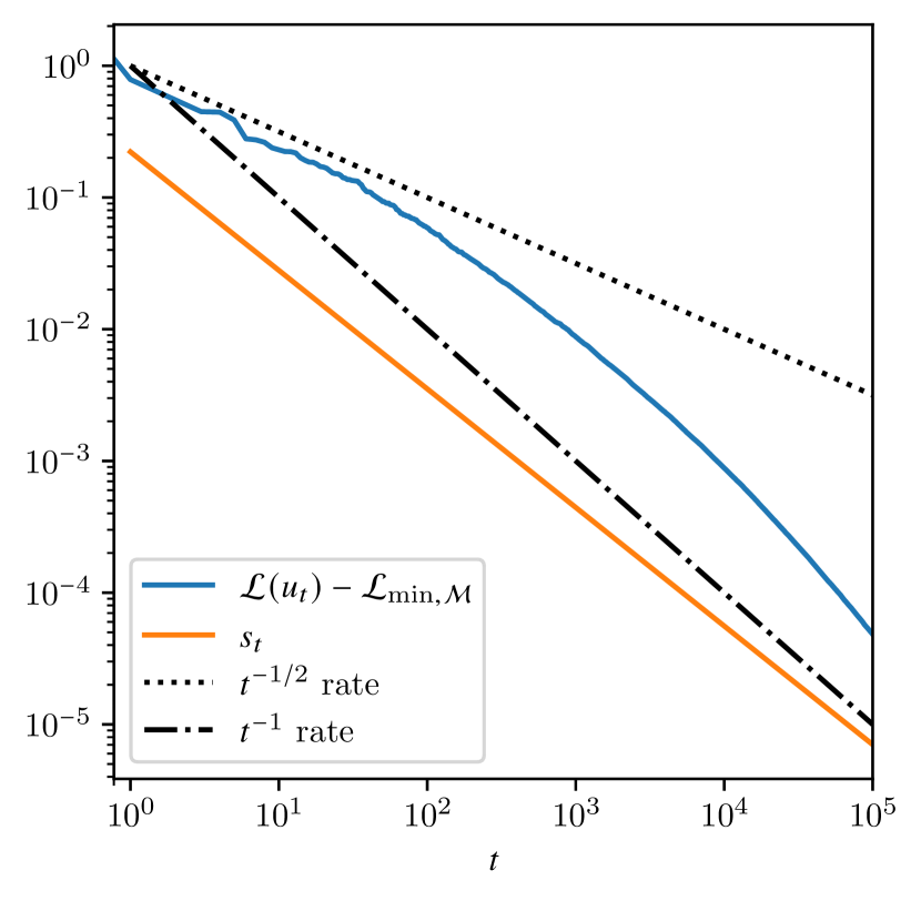
(a) Uniform sampling

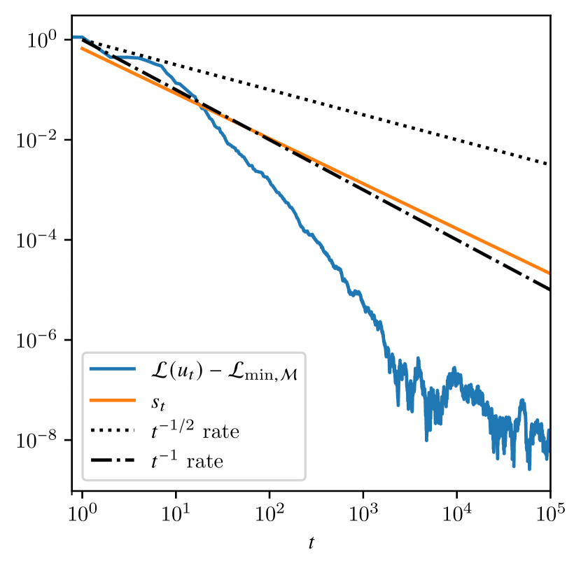
(b) Optimal sampling

Figure 2: Loss error $\mathcal{L}(u_{t})-\mathcal{L}_{\mathrm{min},\mathcal{M}}$, plotted against the number of steps

6.1.2 Exponential convergence for unbiased projections

We consider again the unbiased quasi-projection defined in (11). Corollary 4.9 guarantees that choosing the step size optimally yields exponential convergence up to a fixed precision (in expectation). Figure 3 demonstrates this for the choice $n=1$ and the resulting step size $s_{t}\equiv\tfrac{1}{9}$. We can see a stagnation of the loss in the regime of $\mathcal{L}_{\mathrm{min},\mathcal{M}}$ originating from the use of a constant step size. Since the orthogonal complement $\|(I-P_{t})g_{t}\|$ does not vanish, neither Corollary 4.13 nor Corollary 4.16 apply, and we can not expect convergence.

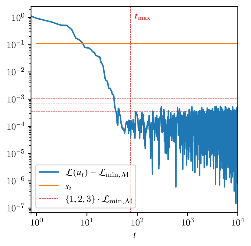
(a) Uniform sampling

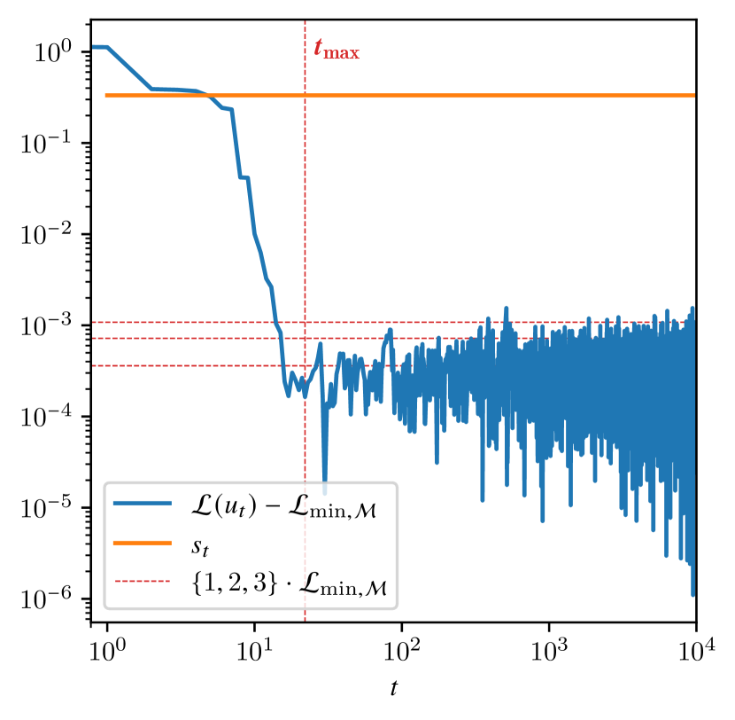
(b) Optimal sampling

Figure 3: Loss error $\mathcal{L}(u_{t})-\mathcal{L}_{\mathrm{min},\mathcal{M}}$, plotted against the number of steps

Since we know that the best approximation error will be attained in expectation after $t_{\mathrm{max}}=22$ steps, we could then switch from the constant step $s_{t}=\tfrac{1}{9}$ to the step size sequence $s_{t}=\tfrac{2}{9}t^{\varepsilon-1}$, guaranteeing sublinear convergence. Figure 4 demonstrates this.

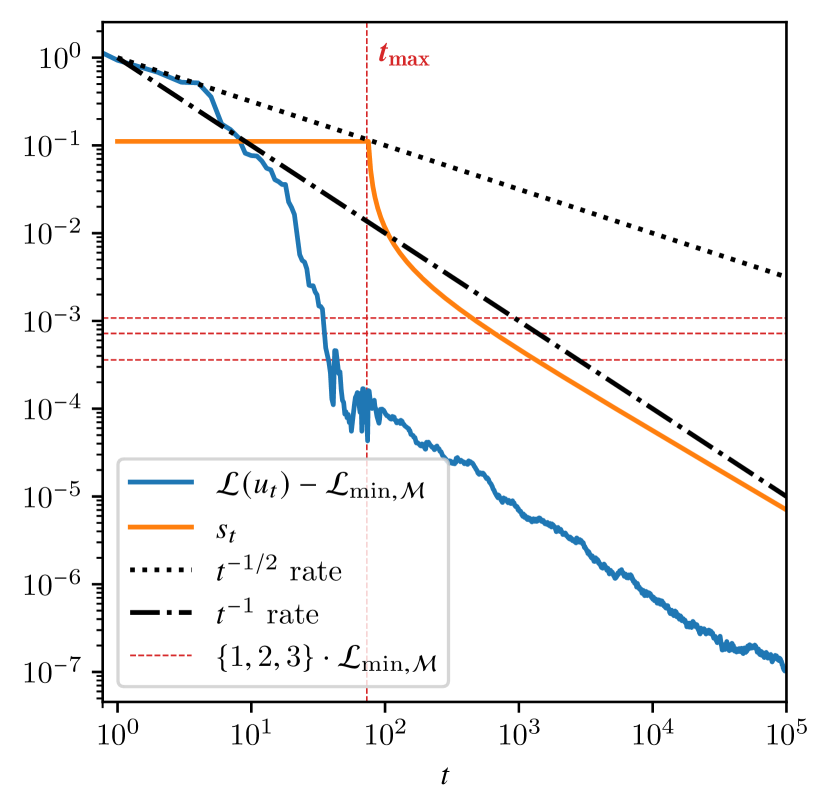
(a) Uniform sampling

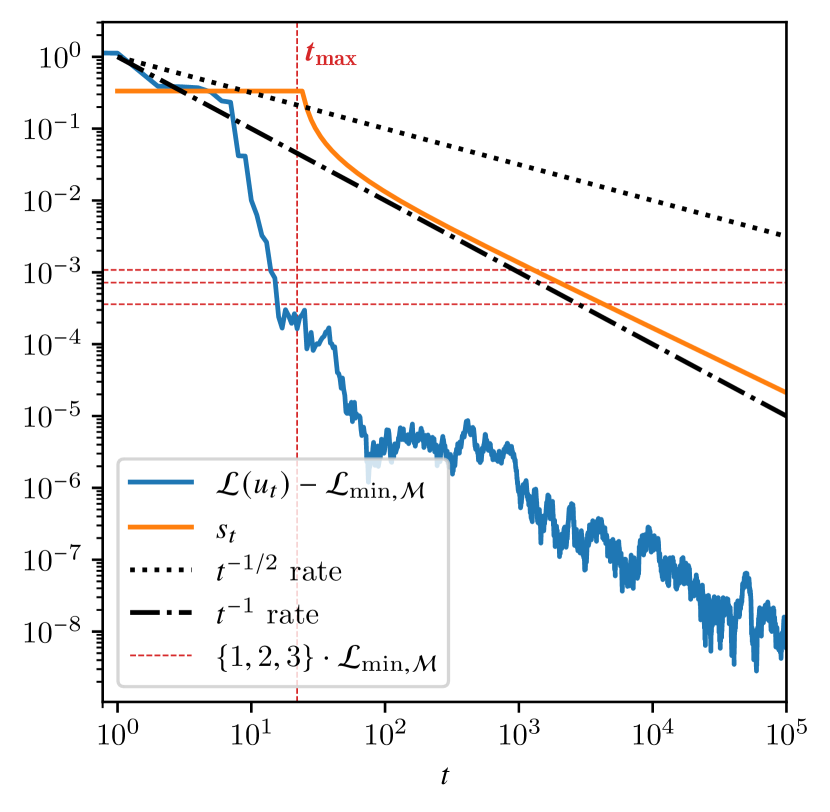
(b) Optimal sampling

Figure 4: Loss error $\mathcal{L}(u_{t})-\mathcal{L}_{\mathrm{min},\mathcal{M}}$, plotted against the number of steps

6.1.3 Convergence for biased projectors

In this section, we consider two different types of projectors

1. stable quasi-projections (11) and

2. least squares projections (14).

The samples are drawn as to guarantee the stability condition (15). To do this, we use conditional sampling with an oversampling factor of $2$, i.e. $n=2d_{t}=6$. This makes the least squares projection well-defined and numerically stable. However, it also induces a bias. As discussed in Remark 4.2, this will produce an algorithm that converges up to the bias (27). This can be rewritten as

$$\mathcal{L}(u_{t})-\mathcal{L}_{\mathrm{min},\mathcal{M}}\leq c_{\mathrm{bias},2}^{2}\mathcal{L}_{\mathrm{min},\mathcal{M}},$$ (61)

which is demonstrated in Figure 5. Note that while the bias introduced in the conditional stable quasi-projection and the least square projection leads to stagnation, as illustrated in Figure 5, the developed quasi-projection strategy (without conditioning) does not stagnate (cf. Figures 2 and 4).

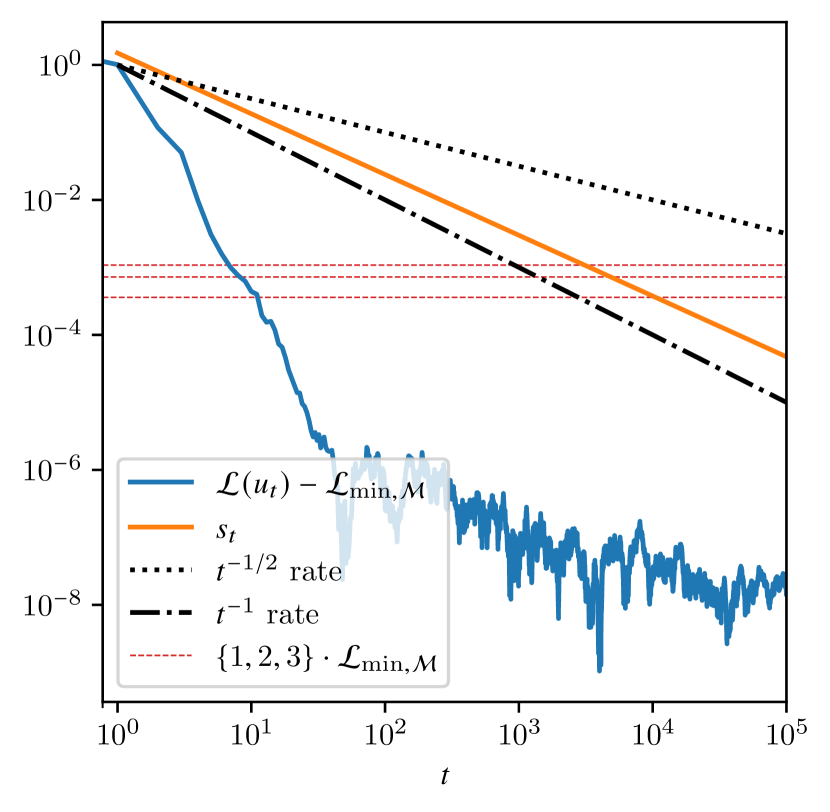
(a) Conditionally stable quasi-projection

(b) Least squares projection

Figure 5: Loss error $\mathcal{L}(u_{t})-\mathcal{L}_{\mathrm{min},\mathcal{M}}$, plotted against the number of steps

Since the empirical Gramian is close to the identity, we would expect both the projection and the quasi-projection to be close to the orthogonal projection. In this case, we could use the deterministically optimal step size $s_{t}\equiv 1$ and achieve convergence in a single iteration. This is demonstrated for four levels of stability in Figure 6.

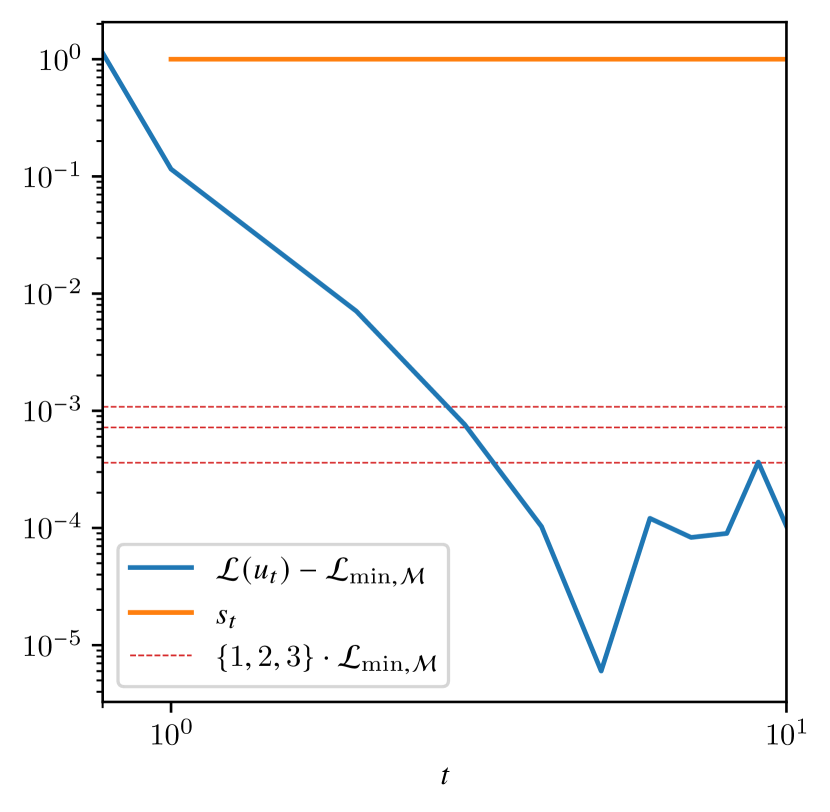
(a) Quasi-projection, $\delta=\tfrac{1}{2}$

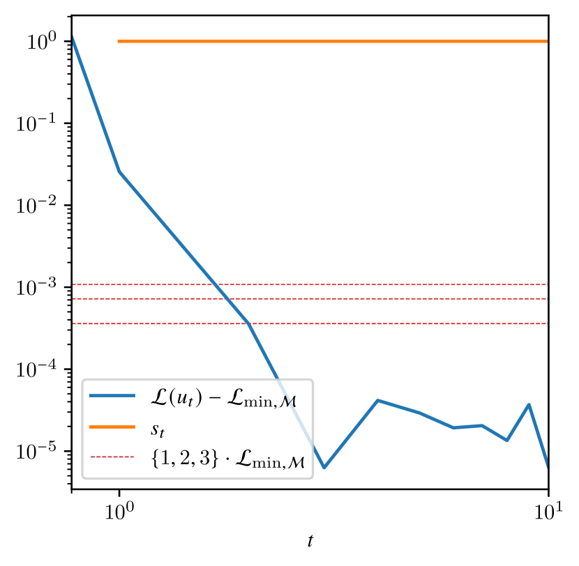
(b) Quasi-projection, $\delta=\tfrac{1}{4}$

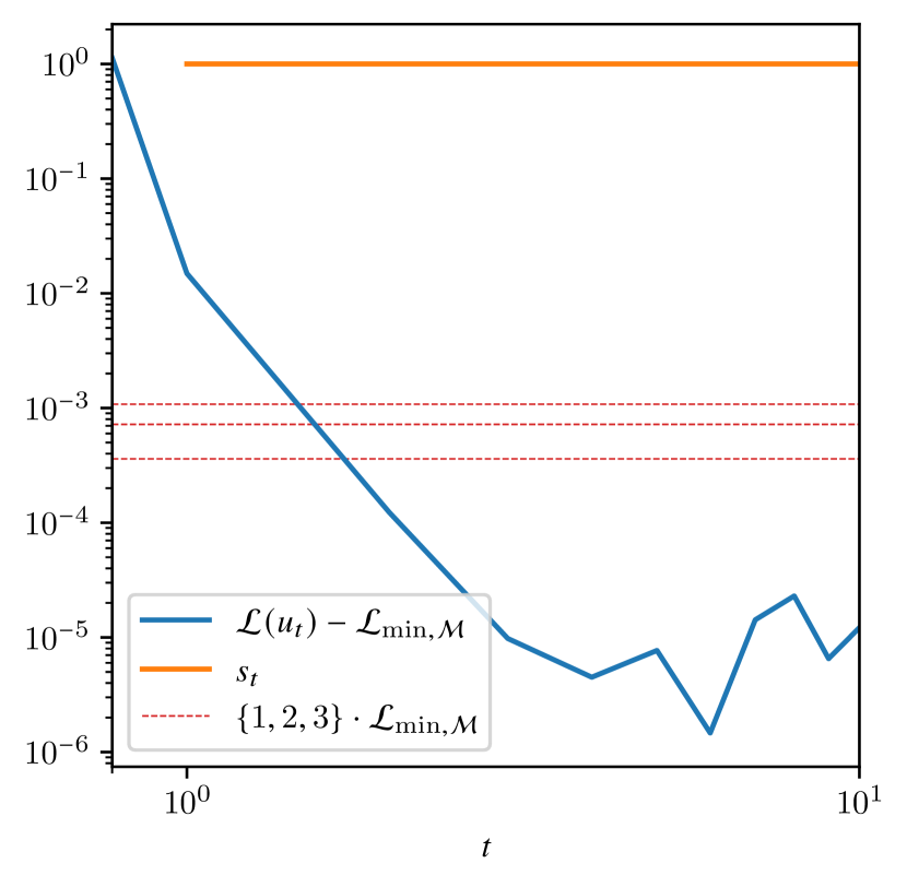
(c) Quasi-projection, $\delta=\tfrac{1}{8}$

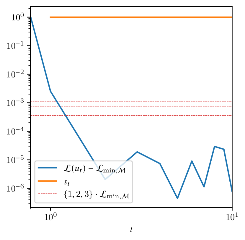
(d) Quasi-projection, $\delta=\tfrac{1}{16}$

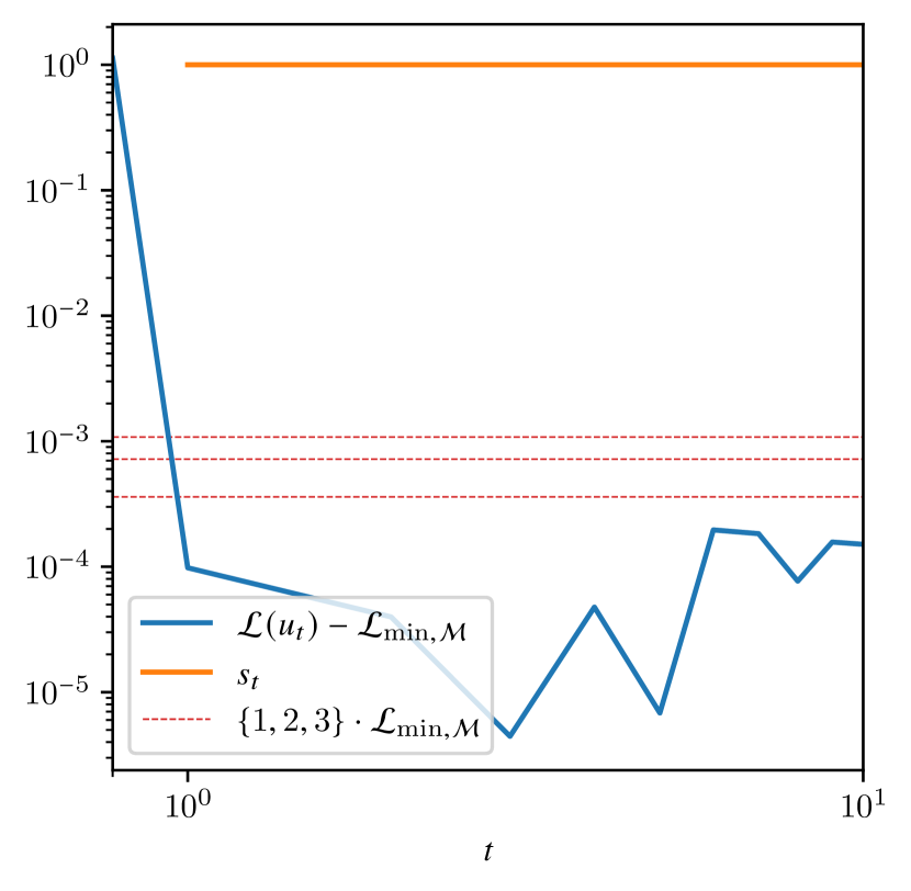
(e) LS projection, $\delta=\tfrac{1}{2}$

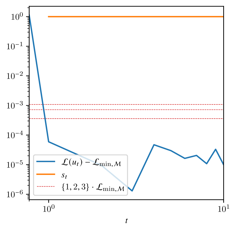
(f) LS projection, $\delta=\tfrac{1}{4}$

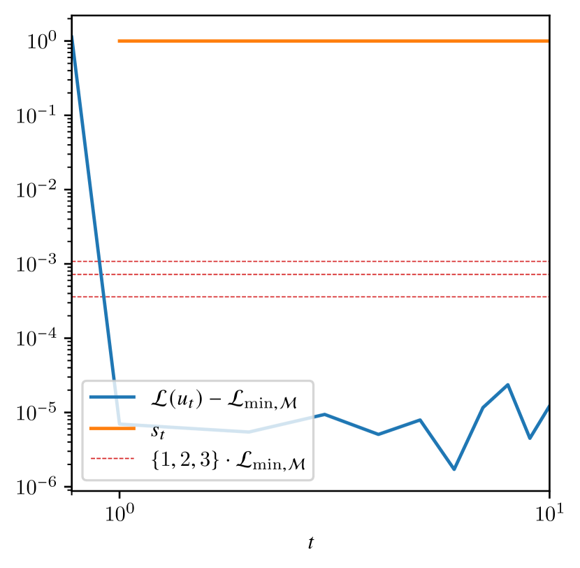
(g) LS projection, $\delta=\tfrac{1}{8}$

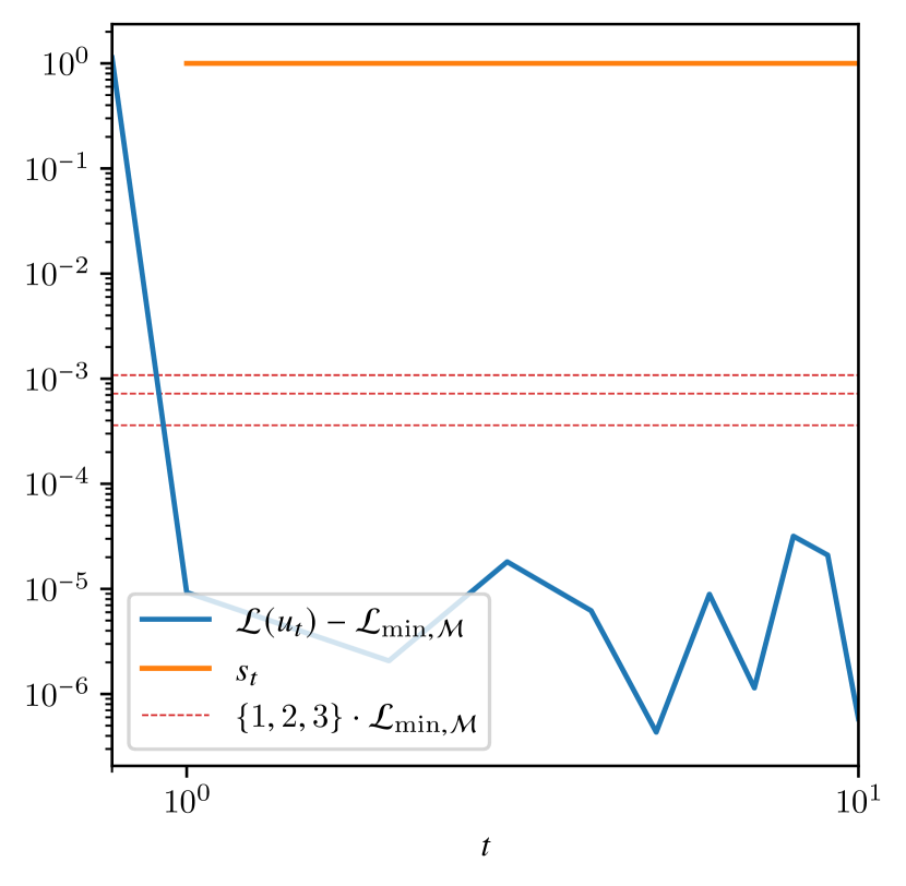
(h) LS projection, $\delta=\tfrac{1}{16}$

Figure 6: Loss error $\mathcal{L}(u_{t})-\mathcal{L}_{\mathrm{min},\mathcal{M}}$, plotted against the number of steps

6.2 Linear approximation on unbounded domains

This subsection considers for $\rho$ the Gaussian distribution on $\mathbb{R}$. We again aim to approximate the target function $u(x)=\exp(x)$. The linear space $\mathcal{V}$ is the space of polynomials of degree less than $6$, and we choose for $\mathcal{B}_{t}$ the first $7$ Hermite polynomials. We choose $\mathcal{M}=\mathcal{V}$ and $\mathcal{T}_{t}\equiv\mathcal{V}$ as well as $R_{t}(v):=v$. Here $\mathcal{L}_{\mathrm{min},\mathcal{M}}\approx 3.1\cdot 10^{-4}$. As before, the strong Polyak-Łojasiewicz property holds with $\lambda=1$ and the retraction error is controlled by $C_{\mathrm{R}}=0$ for any $r>0$. For the empirical operator $P_{t}^{n}$, we choose the unbiased quasi-projection defined in (11). However, as discussed in section 2.2, the variance constant $k_{t}$ is unbounded when the weight function is chosen constant ($w_{t}\equiv 1$). Figure 7 contrasts the uncontrolled behaviour of unweighted SGD with the sublinear convergence rate guaranteed for the optimal weight function in Corollary 4.16.

This section also highlights another very important aspect of SGD. People might think that the Gramian $G$ may be well estimated by Monte Carlo just because the sought function $u$ is smooth. As illustrated in Figure 7, this is by no means the case! We have to use optimal sampling in order to promote stability of the stochastic gradient.

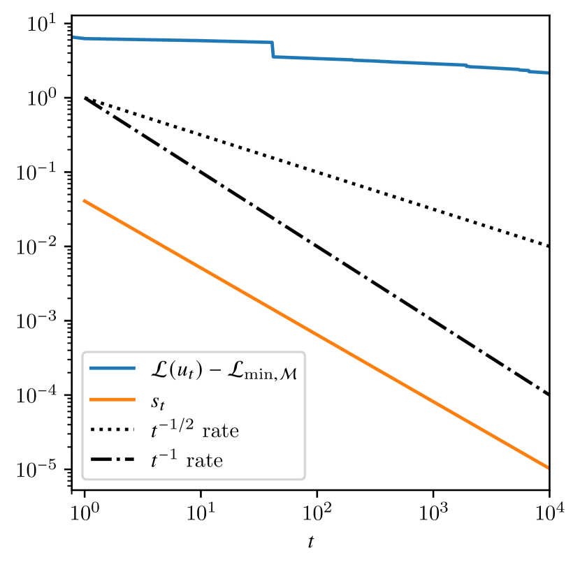
(a) Gaussian sampling, $n=1$

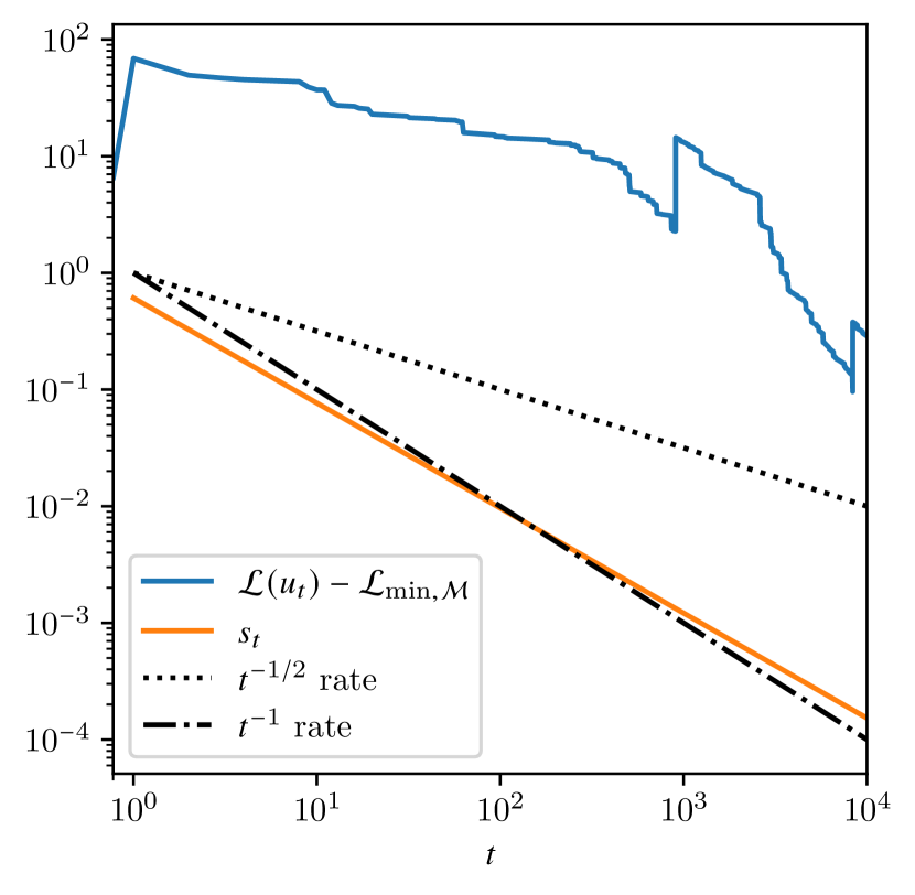
(b) Gaussian sampling, $n=21$

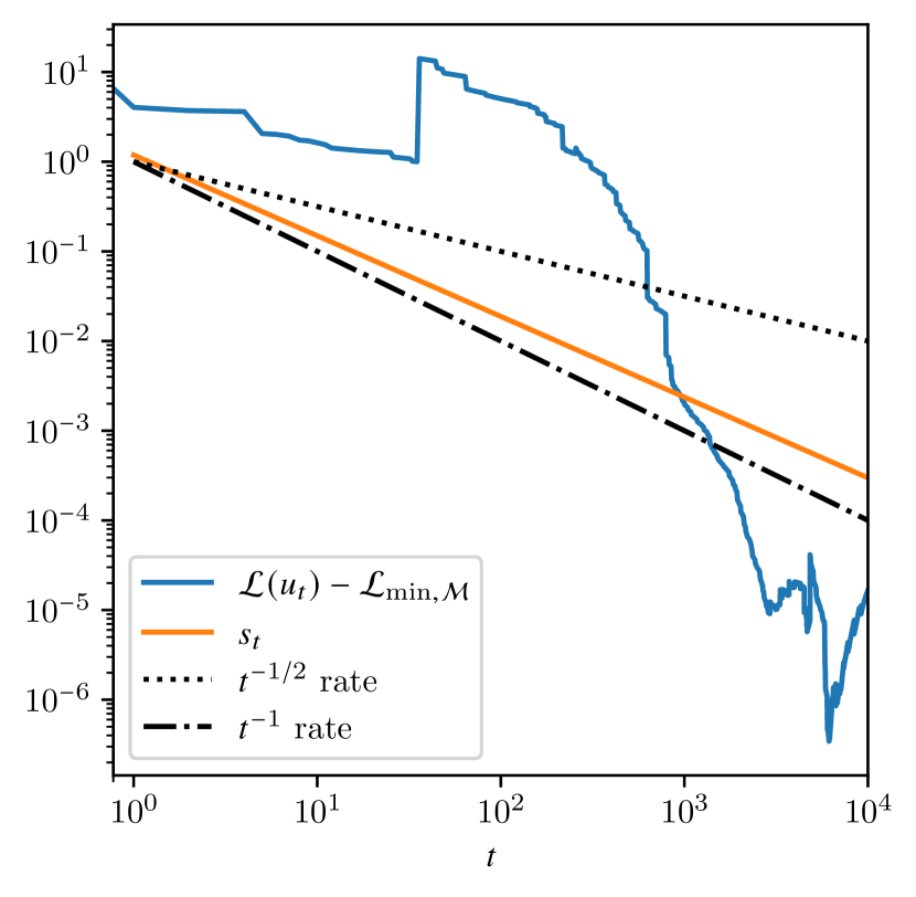
(c) Gaussian sampling, $n=70$

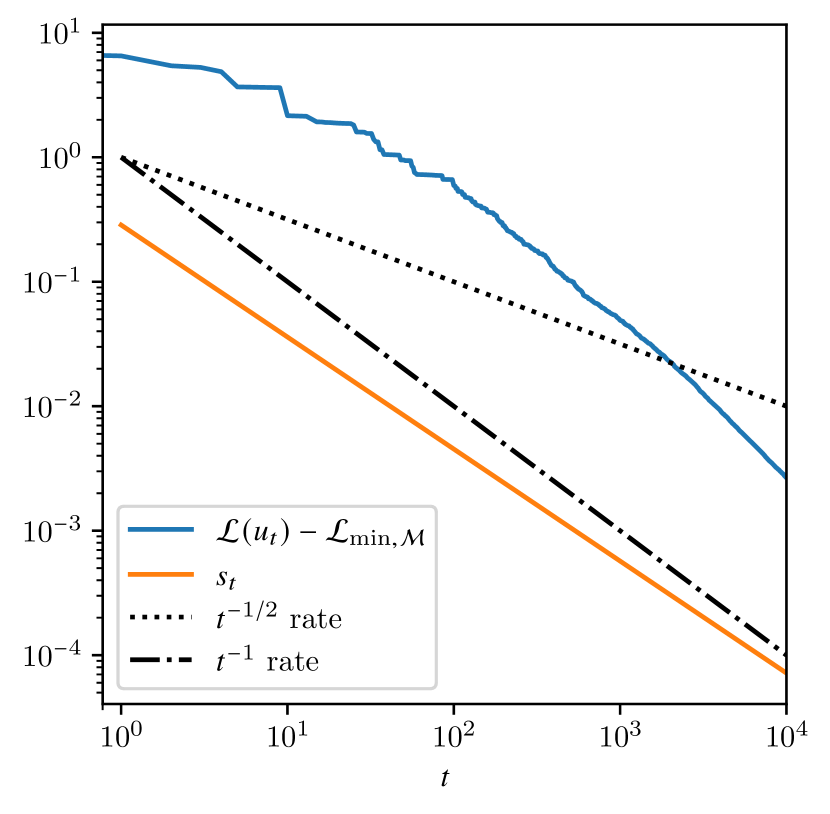
(d) Optimal sampling, $n=1$

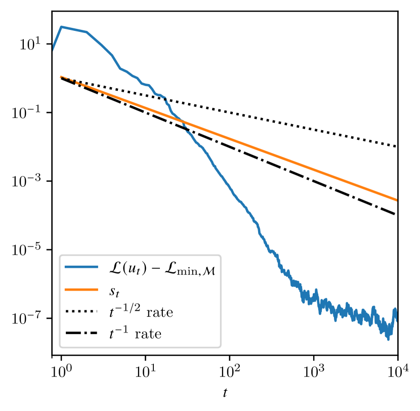
(e) Optimal sampling, $n=7$

Figure 7: Loss error $\mathcal{L}(u_{t})-\mathcal{L}_{\mathrm{min},\mathcal{M}}$, plotted against the number of steps

6.3 Shallow neural networks

As a final example, we consider model classes of shallow neural networks. For a differentiable activation function $\sigma\colon\mathbb{R}\to\mathbb{R}$, we define the shallow network $\Phi_{\theta}\colon\mathcal{X}=\mathbb{R}^{n}\to\mathbb{R}$ of width $m\in\mathbb{N}$ and with parameters $\theta:=(A_{1},b_{1},A_{0},b_{0})\in\Theta:=\mathbb{R}^{1\times m}\times\mathbb{R}\times\mathbb{R}^{m\times n}\times\mathbb{R}^{m}$ by

$$\Phi_{(A_{1},b_{1},A_{0},b_{0})}(x)=A_{1}\sigma(A_{0}x+b_{0})+b_{1}.$$

As a model class, we thus define

$$\mathcal{M}:=\{\Phi_{\theta}\,:\,\theta\in\Theta\}.$$

Some basic properties of this function class are presented in appendix F. We present these properties for general $n\in\mathbb{N}$ to showcase the applicability of our theory in the broader setting. However, for the sake of simplicity and ease of implementation, we restrict the experiments to the case $n=1$.

For the linearisations, we choose $\mathcal{T}_{t}=\mathcal{T}_{\Phi_{\theta_{t}}}$, as defined in appendix F.

Since $u_{t}$ can be represented in the parameter space and $P_{t}^{n}g_{t}$ is associated with a correction in the parameter space, we can define the retraction operator $R_{t}$ as a simple update in the parameter space, as it is usually performed when learning neural networks.

To see that this retraction satisfies assumption (CR), recall that $u_{t+1}=R_{t}(\bar{u}_{t+1})$ and $\bar{u}_{t+1}=u_{t}-s_{t}P_{t}^{n}g_{t}$ with $g_{t}=\nabla\mathcal{L}(u_{t})$. Since $\mathcal{L}$ is $L$-smooth, we can assume that it is locally Lipschitz continuous, i.e. that for every radius $r$ there exists a constant $\mathrm{Lip}_{t}(r)$ such that for all $v,w\in\mathcal{H}$ with $\|v-w\|\leq r$

$$|\mathcal{L}(v)-\mathcal{L}(w)|\leq\mathrm{Lip}_{t}(r)\|v-w\|.$$ (62)

A general formula for the local Lipschitz constant $\mathrm{Lip}_{t}(r)$ of the $L$-smooth loss $\mathcal{L}$ is provided in the subsequent Lemma 6.1 and depends on the knowledge of $\|\nabla\mathcal{L}(v)\|$.

Lemma 6.1.

Let $v$ fixed, then for any $r>0$ it holds that $\mathrm{Lip}_{t}(r)\leq\|\nabla\mathcal{L}(v)\|+Lr$.

Proof.

Suppose that $v,w\in\mathcal{H}$ satisfy $\|v-w\|\leq r$ and let $f:[0,1]\to\mathbb{R}$ be defined by $f(t)=\mathcal{L}(\gamma(t))$ with $\gamma(t)=tv+(1-t)w$. The mean value theorem guarantees that there exists $\eta\in(0,1)$ such that

$$\lvert\mathcal{L}(v)-\mathcal{L}(w)\rvert=\lvert f(1)-f(0)\rvert=f^{\prime}(\eta)=(\nabla\mathcal{L}(\gamma(\eta)),v-w)\leq\|\nabla\mathcal{L}(\gamma(\eta))\|\|v-w\|.$$

Since $\mathcal{L}$ is $L$-smooth, the reverse triangle inequality implies $\|\nabla\mathcal{L}(\gamma(\eta))\|\leq\|\nabla\mathcal{L}(v)\|+L\|v-\gamma(\eta)\|\leq\|\nabla\mathcal{L}(v)\|+Lr$. This implies

$$\lvert\mathcal{L}(v)-\mathcal{L}(w)\rvert \leq(\|\nabla\mathcal{L}(v)\|+Lr)\|v-w\|.\qed$$ (63)

Since for the least squares functional $\|\nabla\mathcal{L}(v)\|=\sqrt{2\mathcal{L}(v)}$, we can estimate this constant by a cumulative mean or an exponentially weighted moving average. Inserting $v=u_{t+1}$ and $w=\bar{u}_{t+1}$ into equation (62) and using Lemma 6.1, we can write

$$|\mathcal{L}(u_{t+1})-\mathcal{L}(\bar{u}_{t+1})|\leq\mathrm{Lip}_{t}(\|u_{t+1}-\bar{u}_{t+1}\|)\|u_{t+1}-\bar{u}_{t+1}\|=(\sqrt{2\mathcal{L}(\bar{u}_{t+1})}+\|u_{t+1}-\bar{u}_{t+1}\|)\|u_{t+1}-\bar{u}_{t+1}\|.$$ (64)

Since $\mathcal{L}(\bar{u}_{t+1})\leq\mathcal{L}(u_{t})$ with high probability and since $\mathcal{L}(u_{t})=\tfrac{1}{2}\|u-u_{t}\|^{2}\approx\tfrac{1}{2}\|u-u_{t}\|_{n}^{2}$, we define the estimate

$$\lambda_{t}:=\frac{1}{2}\|u-u_{t}\|_{n}^{2},$$

where the initial value $\lambda_{0}$ has to be estimated once for the initial guess. With this estimate, with high probability, we have

$$|\mathcal{L}(u_{t+1})-\mathcal{L}(\bar{u}_{t+1})|\leq(\sqrt{2\lambda_{t}}+\varepsilon(s))\varepsilon(s),$$ (65)

where $\varepsilon(s):=\|u_{t+1}-\bar{u}_{t+1}\|=\|R(u_{t}+sP_{t}^{n}g_{t})-(u_{t}+sP^{n}_{t}g_{t})\|$ is the retraction error for step size $s$. Another choice for $\lambda_{t}$ is to take a moving average like $\lambda_{t}=\frac{1}{2}\lambda_{t-1}+\frac{1}{4}\|u-u_{t}\|_{n}^{2}$ to reduce the variance of the estimate $\lambda_{t}$ of $\mathcal{L}(u_{t})$. Note that since $u_{t+1}$ and $\bar{u}_{t+1}$ are shallow neural networks, the norm $\varepsilon(s)$ can be computed analytically. Assumption (CR) is hence satisfied with $C_{\mathrm{R}}=0$ and

$$\beta_{t}(s):=\mathrm{Lip}_{t}(\sqrt{2\lambda_{t}}+\varepsilon(s))\varepsilon(s).$$

With this interpretation, we can choose the step size $s_{t}$ as to maximise the descent factor $\sigma$ while satisfying a given bound on this bias term $\beta_{t}(s_{t})\leq\beta_{t}$ for an a priori chosen sequence $\beta_{t}$. Note, however, that in this case, the resulting step size $s_{t}$ is no longer adapted to the filtration $\mathcal{F}_{t}$ (since it depends on the update direction $P_{t}^{n}g_{t}$) and that the bound $\beta_{t}(s_{t})\leq\beta_{t}$ gives a bound for the step size. This means that $\beta_{t}$ must not decrease too quickly as we need $s\not\in\ell^{1}$. Under certain regularity assumptions of $\theta\mapsto\Phi_{\theta}$, this gives the condition $\beta_{t}\not\in\ell^{2}$, such as $\beta_{t}=s_{\mathrm{opt}}t^{-1/2}$.

As a final adaptation to increase the convergence rate, we argue that the retraction error $\beta_{t}(s_{t})$ should always be smaller than the current loss estimate $\lambda_{t}$ and hence define

$$\beta_{t}:=\min\{\lambda_{t},s_{\mathrm{opt}}t^{-1/2}\}.$$ (66)

Experiments

In the following, we list some plots for the approximation of $u(x):=\sin(2\pi x)$ on the interval $[-1,1]$ by a shallow neural network of width $m=20$. The activation function is the RePU $\sigma(x):=\max\{x,0\}^{2}$ and the linear spaces are chosen as described above ($\mathcal{T}_{t}:=\mathcal{T}_{\Phi_{\theta_{t}}}$). All experiments use $n=10m=200$ sample points per step. Recall that $s_{\mathrm{opt}}$ is the optimal (linear) step size and maximises $\sigma(\raisebox{0.0pt}{\,$\bullet$}\,,0)$. The following experiments were performed.

1. $P_{t}^{n}$ is the least squares projection with optimal sampling and stability constant $\delta=\tfrac{1}{2}$. The step size is chosen such that $\beta_{t}(s_{t})\leq\beta_{t}$ with $\beta_{t}$ defined as in (66). The results are presented in Figure 8.

2. $P_{t}^{n}$ is the least squares projection with optimal sampling and stability constant $\delta=\tfrac{1}{2}$. The step size is chosen as $s_{t}:=s_{\mathrm{opt}}t^{-1/2}$. The results are presented in Figure 9.

3. $P_{t}^{n}$ is the quasi-projection with optimal sampling and without conditioning. The step size is chosen such that $\beta_{t}(s_{t})\leq\beta_{t}$ with $\beta_{t}$ defined as in (66). The results are presented in Figure 10.

4. We compare these to a standard SGD. $P_{t}^{n}$ is the non-projection with uniform sampling. The step size is chosen as $s_{t}:=s_{\mathrm{opt}}t^{-1/2}$. The results are presented in Figure 11.

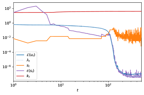
Figure 8: Loss $\mathcal{L}(u_{t})$ for NGD with optimal sampling, least squares projection and adaptive step sizes, plotted against the number of steps

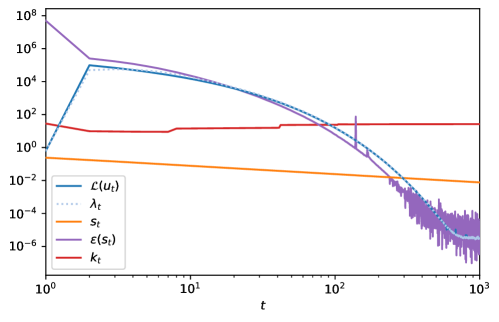
Figure 9: Loss $\mathcal{L}(u_{t})$ for NGD with optimal sampling, least squares projection and deterministically decreasing step sizes, plotted against the number of steps

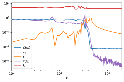
Figure 10: Loss $\mathcal{L}(u_{t})$ for NGD with optimal sampling, quasi-projection and adaptive step sizes, plotted against the number of steps

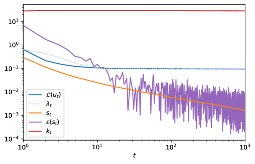
Figure 11: Loss $\mathcal{L}(u_{t})$ for SGD with uniform sampling and deterministically decreasing step sizes, plotted against the number of steps

7 Conclusion and Outlook

This work analyses a natural gradient descent-type algorithm where the descent directions are defined in terms of empirical estimates of the projected gradients. The consideration of potentially nonlinear model classes within the minimisation problem leads to the introduction of a retraction operator. We discuss several projection estimators based on optimal sampling strategies that satisfy certain bias and variance bounds. In particular, we show these bounds for quasi-projections, least squares projections and their extension based on determinantal point processes. The bias and variance bounds for the projection estimator, a control on the retraction error, as well as the Lipschitz-smoothness and (strong) Polyak-Łojasiewicz conditions then enter the convergence analysis. This results in convergence rates in (conditional) expectation and almost surely. Under the assumption of a classic Polyak-Łojasiewicz condition on the loss functional, we prove that the convergence depends on the ratio of the norms of the gradient and its projection. This ratio could be controlled by adaptive model class enrichment, which will be discussed for particular model classes, such as low-rank tensor formats, in a forthcoming work. Numerical experiments confirm the theoretical findings for least square problems based on linear model classes on bounded and unbounded domains and shallow neural networks.

Appendix A Leibniz integral rule

Proposition A.1 (Leibniz integral rule).

Let $\mathcal{V}$ be a Banach space and $(\mathcal{X},\Sigma,\rho)$ be a measure space. Suppose that $\ell:\mathcal{V}\times\mathcal{X}\to\mathbb{R}$ satisfies the following conditions:

1. The function $\ell(v;\raisebox{0.0pt}{\,$\bullet$}\,):\mathcal{X}\to\mathbb{R}$ is Lebesgue integrable for each $v\in\mathcal{V}$.

2. The function $\ell(\raisebox{0.0pt}{\,$\bullet$}\,;x):\mathcal{V}\to\mathbb{R}$ is Fréchet differentiable for almost all $x\in\mathcal{X}$.

3. There exists a Lebesgue integrable function $\alpha:\mathcal{X}\to\mathbb{R}$ such that $\|D_{v}\ell(v;x)\|_{\mathcal{V}^{*}}\leq\alpha(x)$ for all $v\in\mathcal{V}$ and almost all $x\in\mathcal{X}$.

Then, for all $v\in\mathcal{V}$ and $h\in\mathcal{V}$.

$$\left\langle D_{v}\left(\int\ell(v;x)\,\mathrm{d}{\rho(x)}\right),h\right\rangle=\int\langle D_{v}\ell(v;x)h\rangle\,\mathrm{d}{\rho(x)}.$$ (67)

Proof.

See [28]. ∎

Corollary A.2.

Consider a loss function

$$\mathcal{L}(v):=\int\ell(v;x)\,\mathrm{d}{\rho(x)}$$

with $\ell$ satisfying the conditions of Proposition A.1 and $\ell(v;x)=\tilde{\ell}(v(x);x)$ with $\tilde{\ell}:\mathbb{R}\times\mathcal{X}\to\mathbb{R}$. Let $\tilde{\ell}^{\prime}$ denote the derivative of $\ell^{\prime}$ with respect to its first argument. Then the gradient of $\mathcal{L}$ in $L^{2}(\rho)$ is given by

$$\nabla_{v}\mathcal{L}(v)=\tilde{\ell}^{\prime}(v(\raisebox{0.0pt}{\,$\bullet$}\,);\raisebox{0.0pt}{\,$\bullet$}\,).$$

Proof.

By Proposition A.1, it holds for any $v,h\in L^{2}(\rho)$, that

$$(\nabla_{v}\mathcal{L}(v),h) =\langle D_{v}\mathcal{L}(v),h\rangle=\int\langle D_{v}\ell(v;x),h\rangle\,\mathrm{d}{\rho(x)}=\int\tilde{\ell}^{\prime}(v(x);x)h(x)\,\mathrm{d}{\rho(x)}=(\tilde{\ell}^{\prime}(v(\raisebox{0.0pt}{\,$\bullet$}\,);\raisebox{0.0pt}{\,$\bullet$}\,),h).\qed$$ (68)

Appendix B Non- and quasi-projection

In this section, we let $\mathcal{B}_{t}=\{b_{1},...,b_{d}\}$ be a generating system of the $\mathcal{F}_{t}$-measurable space $\mathcal{T}_{t}$ of dimension $d_{t}\leq d$. We let $G\in\mathbb{R}^{d\times d}$ be the corresponding Gramian matrix, with $G_{kl}:=(b_{k},b_{l})$. When $\mathcal{B}_{t}$ is an orthonormal basis, which is the case for quasi-projection, we have $d=d_{t}$ and $G$ is equal to the identity matrix. We let $\lambda_{*}(G)$ denote the smallest strictly positive eigenvalue of $G$, and $\lambda^{*}(G)$ denote the largest eigenvalue of $G$. The subsequent lemmas are generalisations of the basic results from [11] and [45].

Lemma B.1.

Assume that $x_{1},\ldots,x_{n}$ are i.i.d. samples from $\mu_{t}$ given $\mathcal{F}_{t}$ and let $P_{t}^{n}$ the non-projection or quasi-projection defined in (9) or (11) respectively. Then, it holds for any $g\in\mathcal{H}$ that

$$\mathbb{E}\left[(g,P_{t}^{n}g)\mid\mathcal{F}_{t}\right] \geq\lambda_{*}(G)\|P_{t}g\|^{2}.$$ (69)

This bound is tight, and equality holds when $G$ is the identity matrix.

Proof.

Using linearity, we can compute

$$\mathbb{E}\left[P^{n}_{t}g\,\big{|}\,\mathcal{F}_{t}\right]=\mathbb{E}\left[\sum_{k=1}^{d}(g,b_{k})_{n}b_{k}\,\Bigg{|}\,\mathcal{F}_{t}\right]=\sum_{k=1}^{d}\mathbb{E}\left[(g,b_{k})_{n}\,\big{|}\,\mathcal{F}_{t}\right]b_{k}=\sum_{k=1}^{d}(g,b_{k})b_{k}.$$ (70)

Now let $\eta,\theta\in\mathbb{R}^{d}$ be defined by $\eta_{k}:=(g,b_{k})$ and $\theta:=G^{+}\eta$, with $G^{+}$ the Moore-Penrose pseudo-inverse of $G$, and observe that

$$\mathbb{E}\left[P_{t}^{n}g\mid\mathcal{F}_{t}\right]=\sum_{k=1}^{d}\eta_{k}b_{k}\qquad\text{while}\qquad P_{t}g=\sum_{k=1}^{d}\theta_{k}b_{k}.$$

This means that

$$\mathbb{E}\left[(g,P_{t}^{n}g)\mid\mathcal{F}_{t}\right]=(P_{t}g,\mathbb{E}\left[P_{t}^{n}g\mid\mathcal{F}_{t}\right])=\sum_{k,l=1}^{d}\eta_{k}\theta_{k}(b_{k},b_{l})=\theta^{\intercal}G\eta=\eta^{\intercal}G^{+}G\eta.$$

Let $G=U\Lambda U^{\intercal}$ be the compact spectral decomposition with $U\in\mathbb{R}^{d\times r}$ and $\Lambda\in\mathbb{R}^{r\times r}$ and let $\lambda_{*}:=\min\operatorname{diag}(\Lambda)=\lambda_{*}(G)>0$. Then $G^{+}=U\Lambda^{-1}U^{\intercal}$ and

$$\eta^{\intercal}G^{+}G\eta =\eta^{\intercal}UU^{\intercal}\eta\geq\lambda_{*}\eta^{\intercal}U\Lambda^{-1}U^{\intercal}\eta=\lambda_{*}\eta^{\intercal}G^{+}\eta=\lambda_{*}\eta^{\intercal}G^{+}GG^{+}\eta=\lambda_{*}\theta^{\intercal}G\theta=\lambda_{*}\|P_{t}g\|^{2}.\qed$$ (71)

Lemma B.2.

Assume that $x_{1},\ldots,x_{n}$ are i.i.d. samples from $\mu_{t}$ given $\mathcal{F}_{t}$ and let $P_{t}^{n}$ be the non-projection or quasi-projection defined in (9) or (11) respectively. Define $G_{kl}:=(b_{k},b_{l})$ and let $\lambda^{*}(G)$ denote the largest eigenvalue of $G$. Moreover, let $\mathfrak{K}_{t}(x):=\lambda^{*}\left(\sum_{k=1}^{d_{t}}(L_{x}b_{k})(L_{x}b_{k})^{\intercal}\right)$ and $k_{t}:=\|w\mathfrak{K}_{t}\|_{L^{\infty}(\rho)}$. Then, it holds for any $g\in\mathcal{H}$ that

$$\mathbb{E}\left[\|P_{t}^{n}g\|^{2}\,\big{|}\,\mathcal{F}_{t}\right]\leq\Big{(}1-\frac{1}{n}\Big{)}\|P_{t}g\|^{2}+\frac{d_{t}}{n}\|g\|^{2},$$ (72)

and

$$\mathbb{E}\left[\|P_{t}^{n}g\|^{2}\,\big{|}\,\mathcal{F}_{t}\right] \leq\Big{(}1-\frac{1}{n}\Big{)}\lambda^{*}(G)^{2}\|P_{t}g\|^{2}+\frac{\lambda^{*}(G)}{n}\int w(x)\mathfrak{K}(x)\|L_{x}g\|_{2}^{2}\,\mathrm{d}{\rho(x)}$$ (73)

$$\leq\Big{(}1-\frac{1}{n}\Big{)}\lambda^{*}(G)^{2}\|P_{t}g\|^{2}+\frac{\lambda^{*}(G)k_{t}}{n}\|g\|^{2}.$$ (74)

This bound is tight, and equality holds when $G$ is the identity matrix.

Proof.

Let $\eta^{n},\eta,\theta\in\mathbb{R}^{d}$ be defined by $\eta_{k}^{n}:=(g,b_{k})_{n}$, $\eta_{k}:=(g,b_{k})$ and $\theta:=G^{+}\eta$ and recall that

$$\|P_{t}^{n}g\|^{2}=(\eta^{n})^{\intercal}G\eta^{n}\leq\lambda^{*}(G)\|\eta^{n}\|_{2}^{2}\qquad\text{and}\qquad\|\eta\|_{2}^{2}\leq\lambda^{*}(G)(\eta^{\intercal}G^{+}\eta)=\lambda^{*}(G)(\theta^{\intercal}G\theta)=\lambda^{*}(G)\|P_{t}g\|^{2}.$$

We start by considering a single term of the sum $\|\eta^{n}\|_{2}^{2}=\sum_{k=1}^{d}(g,b_{k})_{n}^{2}$. It holds that

$$\mathbb{E}\left[(g,b_{k})_{n}^{2}\,\big{|}\,\mathcal{F}_{t}\right] =\frac{1}{n^{2}}\sum_{i,j=1}^{n}\mathbb{E}\left[w(x_{i})(L_{x_{i}}g)^{\intercal}(L_{x_{i}}b_{k})w(x_{j})(L_{x_{j}}g)^{\intercal}(L_{x_{j}}b_{k})\,\big{|}\,\mathcal{F}_{t}\right]$$ (75)

$$=\begin{multlined}\frac{1}{n^{2}}\sum_{i\neq j=1}^{n}\mathbb{E}\left[w(x_{i})(L_{x_{i}}g)^{\intercal}(L_{x_{i}}b_{k})\,\big{|}\,\mathcal{F}_{t}\right]\mathbb{E}\left[w(x_{j})(L_{x_{j}}g)^{\intercal}(L_{x_{j}}b_{k})\,\big{|}\,\mathcal{F}_{t}\right]\\ +\frac{1}{n^{2}}\sum_{i=1}^{n}\mathbb{E}\left[\left(w(x_{i})(L_{x_{i}}g)^{\intercal}(L_{x_{i}}b_{k})\right)^{2}\,\big{|}\,\mathcal{F}_{t}\right]\end{multlined}\frac{1}{n^{2}}\sum_{i\neq j=1}^{n}\mathbb{E}\left[w(x_{i})(L_{x_{i}}g)^{\intercal}(L_{x_{i}}b_{k})\,\big{|}\,\mathcal{F}_{t}\right]\mathbb{E}\left[w(x_{j})(L_{x_{j}}g)^{\intercal}(L_{x_{j}}b_{k})\,\big{|}\,\mathcal{F}_{t}\right]\\ +\frac{1}{n^{2}}\sum_{i=1}^{n}\mathbb{E}\left[\left(w(x_{i})(L_{x_{i}}g)^{\intercal}(L_{x_{i}}b_{k})\right)^{2}\,\big{|}\,\mathcal{F}_{t}\right]$$ (78)

$$=\frac{n(n-1)}{n^{2}}(g,b_{k})^{2}+\frac{1}{n}\int w(x)(L_{x}g)^{\intercal}(L_{x}b_{k})(L_{x}b_{k})^{\intercal}(L_{x}g)\,\mathrm{d}{\rho(x)},$$ (79)

where the final equality follows from (8). Summing this over $k$ yields

$$\mathbb{E}\left[\|\eta^{n}\|_{2}^{2}\,\big{|}\,\mathcal{F}_{t}\right] =\left(1-\frac{1}{n}\right)\|\eta\|_{2}^{2}+\frac{1}{n}\int w(x)(L_{x}g)^{\intercal}\left(\sum_{k=1}^{d}(L_{x}b_{k})(L_{x}b_{k})^{\intercal}\right)(L_{x}g)\,\mathrm{d}{\rho(x)}$$ (80)

$$\leq\left(1-\frac{1}{n}\right)\|\eta\|_{2}^{2}+\frac{1}{n}\int w(x)\mathfrak{K}(x)\|L_{x}g\|^{2}\,\mathrm{d}{\rho(x)}$$ (81)

$$\leq\left(1-\frac{1}{n}\right)\lambda^{*}(G)\|P_{t}g\|^{2}+\frac{k_{t}}{n}\|g\|^{2},$$ (82)

which ends the proof. ∎

Lemma B.3.

Assume that $x_{1},\ldots,x_{n}$ are i.i.d. samples from $\mu_{t}$ given $\mathcal{F}_{t}$. Let $\mathfrak{K}_{t}(x):=\lambda^{*}\left(\sum_{k=1}^{d}(L_{x}b_{k})(L_{x}b_{k})^{\intercal}\right)$ and $k_{t}:=\|w\mathfrak{K}_{t}\|_{L^{\infty}(\rho)}$. Then, the operator $P_{t}^{n}$ defined in equation (9) satisfies (7) with bias and variance constants

$$c_{\mathrm{bias},1} =\lambda_{*}(G), c_{\mathrm{var},1} =\tfrac{\lambda^{*}(G)^{2}(n-1)+\lambda^{*}(G)k_{t}}{n},$$ (83)

$$c_{\mathrm{bias},2} =0, c_{\mathrm{var},2} =\tfrac{\lambda^{*}(G)k_{t}}{n}.$$ (84)

These bounds are tight.

Proof.

The two bounds $c_{\mathrm{bias},1}=\lambda_{*}(G)$ and $c_{\mathrm{bias},2}=0$ follow directly from Lemma B.1 and Lemma B.2 implies

$$\mathbb{E}\left[\|P_{t}^{n}g\|^{2}\,\big{|}\,\mathcal{F}_{t}\right] \leq\Big{(}1-\frac{1}{n}\Big{)}\lambda^{*}(G)^{2}\|P_{t}g\|^{2}+\frac{\lambda^{*}(G)k_{t}}{n}\|g\|^{2}$$ (85)

$$=\frac{\lambda^{*}(G)^{2}(n-1)+\lambda^{*}(G)k_{t}}{n}\|P_{t}g\|^{2}+\frac{\lambda^{*}(G)k_{t}}{n}\|(I-P_{t})g\|^{2}.\qed$$ (86)

Appendix C Optimal sampling

Lemma C.1.

Let $\{b_{k}\}_{k=1}^{d_{t}}$ be an $\mathcal{H}$-orthonormal basis for the $d_{t}$-dimensional subspace $\mathcal{T}_{t}\subseteq\mathcal{H}$. Let

$$\mathfrak{K}_{t}(x):=\lambda^{*}\left(\sum_{k=1}^{d_{t}}(L_{x}b_{k})(L_{x}b_{k})^{\intercal}\right)$$

and denote by

$$\mathfrak{K}_{\mathcal{T}_{t}}(x):=\sup_{v\in\mathcal{T}_{t}}\frac{\|L_{x}v\|_{2}^{2}}{\|v\|}$$

the generalised inverse Christoffel function (cf. [45]). It holds $\mathfrak{K}_{t}=\mathfrak{K}_{\mathcal{T}_{t}}$. Moreover, define

$$\tilde{\mathfrak{K}}_{t}(x):=\mathrm{trace}\left(\sum_{k=1}^{d_{t}}(L_{x}b_{k})(L_{x}b_{k})^{\intercal}\right).$$

It holds $\mathfrak{K}_{t}\leq\tilde{\mathfrak{K}}_{t}$, with equality if $l=1$ in (5). Moreover, it holds that $\|\tilde{\mathfrak{K}}_{t}\|_{L^{1}(\rho)}=\int\tilde{\mathfrak{K}}_{t}\,\mathrm{d}{\rho}=d_{t}.$

Proof.

Let $B_{x}\in\mathbb{R}^{l\times d_{t}}$ be the matrix with entries $[B_{x}]_{jk}=(L_{x}b_{k})_{j}$. To show the first claim, we compute

$$\mathfrak{K}_{\mathcal{T}_{t}}(x):=\sup_{\begin{subarray}{c}v\in\mathcal{T}_{t}\\ \|v\|=1\end{subarray}}\|L_{x}v\|_{2}^{2}=\sup_{\begin{subarray}{c}\bm{v}\in\mathbb{R}^{d_{t}}\\ \|\bm{v}\|_{2}=1\end{subarray}}\bm{v}^{\intercal}B_{x}^{\intercal}B_{x}\bm{v}=\lambda^{*}(B_{x}^{\intercal}B_{x})=\|B_{x}\|_{2}^{2}=\|B_{x}^{\intercal}\|_{2}^{2}=\lambda^{*}(B_{x}B_{x}^{\intercal})$$

and observe that

$$\mathfrak{K}_{t}(x)=\lambda^{*}\left(\sum_{k=1}^{d_{t}}(L_{x}b_{k})(L_{x}b_{k})^{\intercal}\right)=\lambda^{*}\left(B_{x}B_{x}^{\intercal}\right).$$

The second claim $\mathfrak{K}_{t}(x)\leq\tilde{\mathfrak{K}}_{t}(x)$ is trivial while the last claim follows from

$$\int\tilde{\mathfrak{K}}_{t}\,\mathrm{d}{\rho} =\int\operatorname{trace}(B_{x}^{\intercal}B_{x})\,\mathrm{d}{\rho(x)}=\operatorname{trace}\left(\int B_{x}^{\intercal}B_{x}\,\mathrm{d}{\rho(x)}\right)=\operatorname{trace}\left(I_{d_{t}}\right)=d_{t}.\qed$$ (87)

Appendix D Least squares projection

Lemma D.1.

Let $\delta\in(0,1)$ and assume that $x_{1},\ldots,x_{n}$ are i.i.d. samples from $\mu_{t}$ given $\mathcal{F}_{t}$, conditioned to satisfy the event $\mathcal{S}_{\delta}=[\|I-\hat{G}\|_{2}\leq\delta]$. Moreover, assume the the probability of the event $\mathcal{S}_{\delta}$ is positive $\mathbb{P}(S_{\delta}\,|\,\mathcal{F}_{t})=p_{\mathcal{S}_{\delta}}>0$ and let $\mathfrak{K}_{t}(x):=\lambda^{*}\left(\sum_{k=1}^{d_{t}}(L_{x}b_{k})(L_{x}b_{k})^{\intercal}\right)$ and $k_{t}:=\|w\mathfrak{K}_{t}\|_{L^{\infty}(\rho)}$. Then, the operator $P_{t}^{n}$ defined in equation (14) satisfies (7) with bias and variance constants

$$c_{\mathrm{bias},1}=1,\qquad c_{\mathrm{bias},2}=\tfrac{\sqrt{k_{t}}}{(1-\delta)\sqrt{p_{\mathcal{S}_{\delta}}n}},\qquad c_{\mathrm{var},1}=\tfrac{1}{(1-\delta)^{2}p_{\mathcal{S}_{\delta}}}\tfrac{n-1+k_{t}}{n}\qquad\text{and}\qquad c_{\mathrm{var},2}=\tfrac{1}{(1-\delta)^{2}p_{\mathcal{S}_{\delta}}}\tfrac{k_{t}}{n}.$$

Proof.

Conditioned on this event, the empirical Gramian is invertible and

$$\|P_{t}^{n}g\|=\|\hat{G}^{-1}\hat{\zeta}\|_{2}\leq\|\hat{G}^{-1}\|_{2}\|{\hat{\zeta}}\|_{2}\leq\frac{1}{1-\delta}\|\hat{\zeta}\|_{2}.$$ (88)

Since the random variable $\|\hat{\zeta}\|_{2}^{2}$ is non-negative and $\mathbb{P}[\|I-\hat{G}\|\leq\delta]\geq p_{\mathcal{S}_{\delta}}$ by assumption, it holds that

$$\mathbb{E}\left[\|\hat{\zeta}\|_{2}^{2}\,\big{|}\,\mathcal{F}_{t},\mathcal{S}_{\delta}\right]\leq\frac{\mathbb{E}\left[\|\hat{\zeta}\|_{2}^{2}\,\big{|}\,\mathcal{F}_{t}\right]}{p_{\mathcal{S}_{\delta}}}=\frac{1}{p_{\mathcal{S}_{\delta}}}\sum_{k=1}^{d_{t}}\mathbb{E}\left[(g,b_{k})_{n}^{2}\,\big{|}\,\mathcal{F}_{t}\right].$$ (89)

The last term is the norm of the quasi-projection and is bounded by Lemma B.2. This leads to the variance bound

$$\mathbb{E}\left[\|P_{t}^{n}g\|^{2}\,\big{|}\,\mathcal{F}_{t},\mathcal{S}_{\delta}\right]\leq\frac{1}{(1-\delta)^{2}p_{\mathcal{S}_{\delta}}}\left((1-\tfrac{1}{n})\|P_{t}g\|^{2}+\tfrac{k_{t}}{n}\|g\|^{2}\right).$$ (90)

To bound the bias terms, we start by applying Jensen’s inequality to the variance term above to obtain

$$\mathbb{E}\left[\|P_{t}^{n}g\|\,\big{|}\,\mathcal{F}_{t},\mathcal{S}_{\delta}\right]\leq\mathbb{E}\left[\|P_{t}^{n}g\|^{2}\,\big{|}\,\mathcal{F}_{t},\mathcal{S}_{\delta}\right]^{1/2}\leq\frac{1}{(1-\delta)\sqrt{p_{\mathcal{S}_{\delta}}}}\left((1-\tfrac{1}{n})\|P_{t}g\|^{2}+\tfrac{k_{t}}{n}\|g\|^{2}\right)^{1/2}.$$ (91)

Now let $g^{\perp}:=(I-P_{t})g$ and observe that

$$(g,P_{t}^{n}g)=(g,P_{t}g)+(g,(P_{t}^{n}-P_{t})g)=\|P_{t}g\|^{2}+(g,P_{t}^{n}g^{\perp}),$$ (92)

where the inner product can be bounded via Cauchy–Schwarz inequality by

$$\lvert(g,P_{t}^{n}g^{\perp})\rvert=\lvert(P_{t}g,P_{t}^{n}g^{\perp})\rvert\leq\|P_{t}g\|\|P_{t}^{n}g^{\perp}\|.$$ (93)

Combining the last three equations yields

$$\mathbb{E}\left[(g,P_{t}^{n}g)\,\big{|}\,\mathcal{F}_{t},\mathcal{S}_{\delta}\right] \geq\|P_{t}g\|^{2}-\tfrac{\sqrt{k_{t}}}{(1-\delta)\sqrt{p_{\mathcal{S}_{\delta}}n}}\|P_{t}g\|\|(I-P_{t})g\|.\qed$$ (94)

Appendix E Bound for $\kappa$ in the setting of recovery

The proof of this result relies on the subsequent basic proposition.

Proposition E.1 (Federer [21]).

Suppose that $\mathcal{M}$ is a manifold and that $\mathcal{T}_{v}$ is the tangent space of $\mathcal{M}$ at $v\in\mathcal{M}$. Assume moreover, that $R_{v}:=\operatorname{rch}(\mathcal{M},v)>0$. Then, if $u\in\mathcal{M}$ and $g=v-u$ it holds that

$$\|g-P_{v}g\|\leq\frac{\|g\|^{2}}{2R_{v}}.$$

A simple, geometric proof of this result can be found in [7, Theorem 7.8 (2)] and [45, Appendix B].

Lemma E.2.

Suppose that $\mathcal{M}$ is a differentiable manifold and that $\mathcal{T}_{v}$ is the tangent space of $\mathcal{M}$ at $v\in\mathcal{M}$. Assume moreover, that its reach $R_{v}:=\operatorname{rch}(\mathcal{M},v)>0$. Let $u\in\mathcal{M}$ and consider the risk functional $\mathcal{L}(v):=\tfrac{1}{2}\|u-v\|^{2}$. Then it holds for all $v\in\mathcal{M}$ with $\|u-v\|\leq r\leq R_{v}$ that

$$\frac{\|(I-P_{v})g\|}{\|P_{v}g\|}\leq\frac{r}{R_{v}},$$

where $g:=\nabla\mathcal{L}(v)=v-u$.

Proof.

Recall that by Proposition E.1

$$\|(I-P_{v})g\|\leq\frac{\|g\|^{2}}{2R_{v}}.$$ (95)

Since $\|g\|^{2}=\|P_{v}g\|^{2}+\|(I-P_{v})g\|^{2}$ and $\|(I-P_{v})g\|\leq\|g\|\leq r$, we can write

$$\|(I-P_{v})g\|\leq\frac{\|g\|^{2}}{2R_{v}}=\frac{\|P_{v}g\|^{2}+\|(I-P_{v})g\|^{2}}{2R_{v}}\leq\frac{\|P_{v}g\|^{2}}{2R_{v}}+\frac{\|(I-P_{v})g\|r}{2R_{v}}$$ (96)

and, consequently,

$$\|(I-P_{v})g\|\leq\frac{\|P_{v}g\|^{2}}{2R_{v}-r}\leq\frac{\|P_{v}g\|^{2}}{R_{v}}.$$ (97)

This yields the bound $\frac{\|(I-P_{v})g\|}{\|P_{v}g\|}\leq\frac{\|P_{v}g\|}{R_{v}}\leq\frac{r}{R_{v}}$ and concludes the proof. ∎

Appendix F Shallow neural networks

F.1 Addition

It is well-known that the sum of two shallow neural networks $\Phi_{\theta}$ and $\Phi_{\theta^{\prime}}$ of width $w$ can be represented as another shallow neural network of width $2w$. To see this, observe that

$$\Phi_{(A_{1},b_{1},A_{0},b_{0})}(x)+\Phi_{(A_{1}^{\prime},b_{1}^{\prime},A_{0}^{\prime},b_{0}^{\prime})}(x) =A_{1}\sigma(A_{0}x+b_{0})+b_{1}+A_{1}^{\prime}\sigma(A_{0}^{\prime}x+b_{0}^{\prime})+b_{1}^{\prime}$$ (98)

$$=\underbrace{\begin{bmatrix}A_{1}&A_{1}^{\prime}\end{bmatrix}}_{\eqqcolon A_{1}^{\prime\prime}}\sigma\Bigg{(}\underbrace{\begin{bmatrix}A_{0}\\ A_{0}^{\prime}\end{bmatrix}}_{\eqqcolon A_{0}^{\prime\prime}}x+\underbrace{\begin{bmatrix}b_{0}\\ b_{0}^{\prime}\end{bmatrix}}_{\eqqcolon b_{0}^{\prime\prime}}\Bigg{)}+\underbrace{(b_{1}+b_{1}^{\prime})}_{\eqqcolon b_{1}^{\prime\prime}}$$ (99)

$$=\Phi_{(A_{1}^{\prime\prime},b_{1}^{\prime\prime},A_{0}^{\prime\prime},b_{0}^{\prime\prime})}.$$ (100)

Defining the binary operation $\boxplus$ accordingly, we can thus write $\Phi_{\theta}+\Phi_{\theta^{\prime}}=\Phi_{\theta\boxplus\theta^{\prime}}$.

F.2 Inner products

Denote by $A_{k*}$ the $k$^th row of the matrix $A$ and observe that the $L^{2}(\rho)$-inner product of two shallow neural networks is given by

$$(\Phi_{\theta},\Phi_{\theta^{\prime}})=\begin{multlined}\sum_{k=1}^{m}\sum_{l=1}^{m^{\prime}}A_{1,1k}A^{\prime}_{1,1l}\left(\sigma(A_{0,k*}x+b_{0,k}),\sigma(A_{0,l*}^{\prime}x+b_{0,l}^{\prime})\right)\\ +\sum_{k=1}^{m}A_{1,1k}b^{\prime}_{1}\left(\sigma(\vphantom{A_{0}^{\prime}}A_{0,k*}x+b_{0,k}),1\right)\\ +\sum_{l=1}^{m^{\prime}}b_{1}A^{\prime}_{1,1l}\left(\sigma(A_{0,l*}^{\prime}x+b_{0,l}^{\prime}),1\right).\end{multlined}\sum_{k=1}^{m}\sum_{l=1}^{m^{\prime}}A_{1,1k}A^{\prime}_{1,1l}\left(\sigma(A_{0,k*}x+b_{0,k}),\sigma(A_{0,l*}^{\prime}x+b_{0,l}^{\prime})\right)\\ +\sum_{k=1}^{m}A_{1,1k}b^{\prime}_{1}\left(\sigma(\vphantom{A_{0}^{\prime}}A_{0,k*}x+b_{0,k}),1\right)\\ +\sum_{l=1}^{m^{\prime}}b_{1}A^{\prime}_{1,1l}\left(\sigma(A_{0,l*}^{\prime}x+b_{0,l}^{\prime}),1\right).$$

To compute $(\Phi_{\theta},\Phi_{\theta^{\prime}})$, it hence suffices to compute inner products of the form $\left(\sigma(\alpha^{\intercal}x+\beta),\sigma(\alpha^{\prime\intercal}x+\beta^{\prime})\right)$ and $\left(\sigma(\vphantom{\alpha^{\prime}}\alpha^{\intercal}x+\beta),1\right)$ for given $\alpha,\alpha^{\prime}\in\mathbb{R}^{n}$ and $\beta,\beta^{\prime}\in\mathbb{R}$.

Since the function $\sigma(\alpha^{\intercal}x+\beta)$ varies only in the direction of $\alpha$ and is constant in its orthogonal complement, the inner product $\left(\sigma(\vphantom{\alpha^{\prime}}\alpha^{\intercal}x+\beta),1\right)$ can be recast as a one-dimensional integration problem after a suitable transform of coordinates. Similarly, the product $\sigma(\alpha^{\intercal}x+\beta)\sigma(\alpha^{\prime\intercal}x+\beta^{\prime})$ only varies in the two-dimensional subspace $\operatorname{span}(\alpha,\alpha^{\prime})$ and can thereby be recast as a two-dimensional integration problem.

This allows the computation of norms and distances between shallow neural networks as well as the computation of Gramians of bases of spaces of neural networks. We can then use these Gramians to find orthonormal bases, compute least squares projections and draw optimal samples.

One-dimensional integrals

If $\rho$ is the uniform measure on a convex polytope $\Sigma$ and $\sigma$ is the logistic sigmoid $\sigma(x):=(1+\exp(-x))^{-1}$, explicit formulae for the one-dimensional integrals $\left(\sigma(\alpha^{\intercal}x+\beta),1\right)$ are derived in [35]. Although we believe these formulae can be extended to the two-dimensional integrals, we will consider a simpler example in the following.

Let $\rho$ denote the probability density function of the standard Gaussian measure on $\mathbb{R}^{d}$ for $d\in\mathbb{N}$ chosen appropriately according to context. Note that for any $\alpha\in\mathbb{R}^{n}$ and $\beta\in\mathbb{R}$, we can find an orthogonal matrix $Q\in\mathbb{R}^{n\times n}$, such that $Qe_{1}\propto\alpha$. Therefore, the change-of-variables formula then implies

$$\int_{\mathbb{R}^{n}}\sigma(\alpha^{\intercal}y+\beta)\rho(y)\,\mathrm{d}{y} =\int_{\mathbb{R}^{n}}\sigma(\alpha^{\intercal}Qx+\beta)\rho(Qx)\,\mathrm{d}{x}$$ (101)

$$=\int_{\mathbb{R}}\sigma(\|\alpha\|_{2}x_{1}+\beta)\left(\int_{\mathbb{R}^{n-1}}\rho(Qx)\,\mathrm{d}{(x_{2},\ldots,x_{n})}\right)\,\mathrm{d}{x_{1}}$$ (102)

$$=\int_{\mathbb{R}}\sigma(\|\alpha\|_{2}x_{1}+\beta)\rho(x_{1})\,\mathrm{d}{x_{1}}.$$ (103)

This integral is computable by classical one-dimensional quadrature rules such as Gauß–Hermite quadrature.

Two-dimensional integrals

Let again $\rho$ denote the probability density function of the standard Gaussian measure on $\mathbb{R}^{d}$ for any $d\in\mathbb{N}$ and let $\alpha,\alpha^{\prime}\in\mathbb{R}^{n}$ and $\beta,\beta^{\prime}\in\mathbb{R}$. We can assume that $\alpha$ and $\alpha^{\prime}$ are linearly independent since if this is not the case, we are in the setting of one-dimensional integrals. Under this assumption, we can find an orthogonal matrix $Q\in\mathbb{R}^{n\times n}$, such that $Qe_{1}\propto\alpha$ and $Qe_{2}\propto\alpha^{\prime}-\frac{(\alpha^{\prime},\alpha)}{\|\alpha\|_{2}^{2}}\alpha$. Defining $\gamma_{1}:=\alpha^{\prime\intercal}Qe_{1}$ and $\gamma_{2}:=\alpha^{\prime\intercal}Qe_{2}$, we can again employ the change-of-variables formula to obtain

$$\int_{\mathbb{R}^{n}}\sigma(\alpha^{\intercal}y+\beta)\sigma(\alpha^{\prime\intercal}y+\beta^{\prime})\rho(y)\,\mathrm{d}{y} =\int_{\mathbb{R}^{n}}\sigma(\alpha^{\intercal}Qx+\beta)\sigma(\alpha^{\prime\intercal}Qx+\beta^{\prime})\rho(Qx)\,\mathrm{d}{x}$$ (104)

$$=\begin{multlined}\int_{\mathbb{R}^{2}}\sigma(\|\alpha\|_{2}x_{1}+\beta)\sigma(\gamma_{1}x_{1}+\gamma_{2}x_{2}+\beta^{\prime})\\ \cdot\left(\int_{\mathbb{R}^{n-2}}\rho(Qx)\,\mathrm{d}{(x_{3},\ldots,x_{n})}\right)\,\mathrm{d}{(x_{1},x_{2})}\end{multlined}\int_{\mathbb{R}^{2}}\sigma(\|\alpha\|_{2}x_{1}+\beta)\sigma(\gamma_{1}x_{1}+\gamma_{2}x_{2}+\beta^{\prime})\\ \cdot\left(\int_{\mathbb{R}^{n-2}}\rho(Qx)\,\mathrm{d}{(x_{3},\ldots,x_{n})}\right)\,\mathrm{d}{(x_{1},x_{2})}$$ (107)

$$=\int_{\mathbb{R}^{2}}\sigma(\|\alpha\|_{2}x_{1}+\beta)\sigma(\gamma_{1}x_{1}+\gamma_{2}x_{2}+\beta^{\prime})\rho(x_{1},x_{2})\,\mathrm{d}{(x_{1},x_{2})}.$$ (108)

This integral can be computed by classical two-dimensional Gauß–Hermite quadrature.

F.3 Local linearisation

Analogously to the definition of the tangent space of embedded manifolds, one can define the local linearisation of $\mathcal{M}$ around the network $\Phi_{\theta}$ as

$$\mathcal{T}_{\Phi_{\theta}}:=\operatorname{span}\{\partial_{\theta_{j}}\Phi_{\theta}\,:\,j=1,\ldots,d\},$$

where $\theta\in\mathbb{R}^{1\times m}\times\mathbb{R}\times\mathbb{R}^{m\times n}\times\mathbb{R}^{m}$ is identified with its vectorisation $\operatorname{vec}(\theta)\in\mathbb{R}^{d}$ with $d={m(n+2)+1}$. Since the space $\mathcal{T}_{\Phi_{\theta}}$ is spanned by the partial derivatives

$$\partial_{A_{1,1j}}\Phi_{(A_{1},b_{1},A_{0},b_{0})} =\sigma(A_{0}x+b_{0})_{j},$$ (109)

$$\partial_{b_{1}}\Phi_{(A_{1},b_{1},A_{0},b_{0})} =1,$$ (110)

$$\partial_{A_{0,ij}}\Phi_{(A_{1},b_{1},A_{0},b_{0})} =A_{1,1i}\sigma^{\prime}(A_{0}x+b_{0})_{i}x_{j},$$ (111)

$$\partial_{b_{0,i}}\Phi_{(A_{1},b_{1},A_{0},b_{0})} =A_{1,1i}\sigma^{\prime}(A_{0}x+b_{0})_{i},$$ (112)

it is at most $d$-dimensional and contains $\Phi_{\theta}$. Note, however, that the important derivative $\partial_{A_{0,ij}}\Phi_{(A_{1},b_{1},A_{0},b_{0})}$ can not be expressed directly as a neural network. This is relevant because we want to compute the Gramian according to the theory presented in the previous section. (Note that $\partial_{b_{0,i}}\Phi_{(A_{1},b_{1},A_{0},b_{0})}$ is not a problem because it still exhibits the ridge-structure that is necessary for efficient integration.)

There are two ways to bypass this problem.

1. In the Gaussian setting, we can use the Gaussian integration by parts formula (also known as Isserlis’ theorem or Wick’s probability theorem) to get rid of the additional $x_{j}$-factor.

2. We can approximate the function $\partial_{A_{0,ij}}\Phi_{(A_{1},b_{1},A_{0},b_{0})}$ by a shallow neural network. A straightforward way to do this is to replace the differential with a finite difference approximation with step size $h>0$.

For the sake of simplicity, we choose to opt for the second option. We define the elementary matrices $(E_{ij})_{kl}:=\delta_{ik}\delta_{jl}$ and propose to approximate

$$\partial_{A_{0,ij}}\Phi_{(A_{1},b_{1},A_{0},b_{0})} \approx\tfrac{A_{1,1i}}{h}\left[\sigma((A_{0}+E_{ij}h)x+b_{0})_{i}-\sigma(A_{0}x+b_{0})_{i}\right]$$ (113)

$$\partial_{b_{0,i}}\Phi_{(A_{1},b_{1},A_{0},b_{0})} \approx\tfrac{A_{1,1i}}{h}\left[\sigma(A_{0}x+(b_{0}+e_{i}h))_{i}-\sigma(A_{0}x+b_{0})_{i}\right].$$ (114)

The corresponding linearisation space can then be written as

$$\mathcal{T}_{\Phi_{\theta}}^{h}:=\ \operatorname{span}\left\{\sigma(A_{0}x+b_{0})_{j}\,:\,j=1,\ldots,m\right\}$$ (115)

$$+\ \operatorname{span}\left\{1\right\}$$ (116)

$$+\ \operatorname{span}\left\{\sigma((A_{0}+E_{ij}h)x+b_{0})_{i}\,:\,i=1,\ldots,n,\ j=1,\ldots,m\right\}$$ (117)

$$+\ \operatorname{span}\left\{\sigma(A_{0}x+(b_{0}+e_{j}h))_{i}\,:\,j=1,\ldots,m\right\}.$$ (118)

F.4 Optimal sampling

Let $\{\phi_{j}\}_{j=1,\ldots,d}$ be a generating system of the space $\mathcal{T}_{t}$. Given the Gramian $G$ of this generating system, we can compute an orthonormal basis $\{\psi_{k}\}_{k=1,\ldots,r}$ with $r\leq d$ and

$$\psi_{k}:=\sum_{j=1}^{d}c_{kj}\phi_{j}.$$

Recall that the optimal sampling density of the space $\operatorname{span}\{\psi_{k}\}_{k=1,\ldots,r}$ is given by

$$p(x):=\frac{1}{r}\sum_{k=1}^{r}p_{k}(x)\qquad\text{with}\qquad p_{k}(x):=\psi_{k}^{2}(x)\rho(x).$$

To draw samples from this distribution, we can employ a combination of mixture sampling and sequential conditional sampling. First, we draw an index $k\in[r]$ uniformly at random. Then, we draw a sample from $p_{k}$ by decomposing

$$p_{k}(x)=p_{k}(x_{n}\mid x_{n-1},\ldots,x_{1})\cdots p_{k}(x_{2}\mid x_{1})p_{k}(x_{1}).$$

To compute the marginals, observe that

$$p_{k}(x_{l}\mid x_{l-1},\ldots,x_{1}) =\int\psi_{k}^{2}(x)\rho(x)\,\mathrm{d}{(x_{n},\ldots,x_{l+1})}$$ (119)

$$=\int\left(\sum_{j=1}^{d}c_{kj}\phi_{j}(x)\right)^{2}\rho(x)\,\mathrm{d}{(x_{n},\ldots,x_{l+1})}$$ (120)

$$=\sum_{i,j=1}^{d}c_{ki}c_{kj}\int\phi_{i}(x)\phi_{j}(x)\rho(x)\,\mathrm{d}{(x_{n},\ldots,x_{l+1})}$$ (121)

is a sum of (parametric in $x_{l},\ldots,x_{1}$) two-dimensional integrals, as discussed above. This can be implemented in an efficient, parallelised fashion, taking arrays of sample points $x_{l-1},\ldots,x_{1}\in\mathbb{R}^{N}$ and of evaluation points $x_{l}\in\mathbb{R}^{D}$ and returning the matrix of probabilities $p_{k}(x_{l}\mid x_{l-1},\ldots,x_{1})\in\mathbb{R}^{D\times N}$. This allows us to approximate the (one-dimensional) cumulative distribution function of $p_{k}(x_{l}\mid x_{l-1},\ldots,x_{1})$, which can be used for inverse transform sampling of $x_{l}$.

Appendix G The strong Polyak–Łojasiewicz condition

Definition G.1.

A manifold $\mathcal{M}$ is called geodesically convex if for every two points $v,w\in\mathcal{M}$ there exists a unique geodesic that connects $v$ and $w$.

Definition G.2.

Let $\mathcal{M}$ be geodesically convex. A parameterisation of this geodesic $\gamma_{vw}:[0,T_{vw}]\to\mathcal{M}$ is said to have unit speed if at every point $t\in(0,T_{vw})$ the derivative $\dot{\gamma}(t)\in\mathbb{T}_{\gamma(t)}\mathcal{M}$ satisfies

$$\|\dot{\gamma}(t)\|_{\mathcal{H}}=1,$$

where we identify the bounded linear map $d_{t}\gamma\in\mathcal{L}(\mathbb{R},\mathbb{T}_{\gamma(t)}\mathcal{M})$ with $\dot{\gamma}(t)\in\mathbb{T}_{\gamma(t)}\mathcal{M}$.

Definition G.3.

Let $\mathcal{M}$ be geodesically convex and $\mathcal{L}:\mathcal{M}\to\mathbb{R}$. $\mathcal{L}$ is called $\lambda$-strongly geodesically convex on $\mathcal{M}$, if for every two points $v,w\in\mathcal{M}$ and corresponding unit-speed parameterised geodesic $\gamma_{vw}$, the function $\mathcal{L}\circ\gamma_{vw}:[0,T_{vw}]\to\mathbb{R}$ is $\lambda$-strongly convex in the conventional sense.

Lemma G.4.

Suppose that $\mathcal{M}\subseteq\mathcal{H}$ is a geodesically convex Riemannian submanifold of $\mathcal{H}$ without boundary and let $T_{t}=\mathbb{T}_{u_{t}}\mathcal{M}$ be the tangent space of $\mathcal{M}$ at $u_{t}$. Furthermore assume that $\mathcal{L}_{\mathrm{min},\mathcal{M}}\in\mathbb{R}$ is attained in $\mathcal{M}$. If $\mathcal{L}:\mathcal{M}\to\mathbb{R}$ is $\lambda$-strongly geodesically convex on $\mathcal{M}$, then (SPL) is satisfied.

Proof.

To prove the assertion, let $u\in\mathcal{M}$ be arbitrary and denote by $u_{\mathrm{min},\mathcal{M}}$ the minimum of $\mathcal{L}$ in $\mathcal{M}$. Let $\gamma:=\gamma_{uu_{\mathrm{min},\mathcal{M}}}$ be the unit-speed parameterisation of the geodesic from $u$ to $u_{\mathrm{min},\mathcal{M}}$ and define the function $g:=\mathcal{L}\circ\gamma:[0,T]\to\mathbb{R}$ with $T:=T_{uu_{\mathrm{min},\mathcal{M}}}$. When $\mathcal{L}$ is $\lambda$-strongly geodesically convex on $\mathcal{M}$, then

$$g(t)\geq g(s)+\dot{g}(s)(t-s)+\tfrac{\lambda}{2}(t-s)^{2}$$ (122)

for any $t\in[0,T]$ and $s\in(0,T)$. We now minimise both sides of this equation with respect to $t$. For the left-hand side, this immediately yields $g(T)=\mathcal{L}_{\mathrm{\min},\mathcal{M}}$. To minimise the right-hand side, we compute the first-order necessary optimality condition

$$\dot{g}(s)+\lambda(t-s)=0.$$

Solving this equation for $t$ yields $t=s-\tfrac{1}{\lambda}\dot{g}(s)$. Since minimisation preserves the inequality in equation (122), we can substitute the optimal values that we obtained for each side back into (122). This yields

$$\mathcal{L}_{\mathrm{min},\mathcal{M}}\geq g(s)-\tfrac{1}{\lambda}\dot{g}(s)^{2}+\tfrac{1}{2\lambda}\dot{g}(s)^{2}=g(s)-\tfrac{1}{2\lambda}\dot{g}(s)^{2}.$$ (123)

Let $P_{\dot{\gamma}(s)}$ denote the $\mathcal{H}$-orthogonal projection onto $\operatorname{span}\{\dot{\gamma}(s)\}\subseteq\mathbb{T}_{u}\mathcal{M}$. Since $\gamma$ is a unit-speed parameterisation, the chain rule implies that

$$\dot{g}(s)^{2}=\left(\mathcal{R}(d_{\gamma(s)}\mathcal{L}\circ d_{s}\gamma)\right)^{2}=(\nabla\mathcal{L}(\gamma(s)),\dot{\gamma}(s))_{\mathcal{H}}^{2}=\|P_{\dot{\gamma}(s)}\nabla\mathcal{L}(\gamma(s))\|_{\mathcal{H}}^{2}\leq\|P_{\mathbb{T}_{u}\mathcal{M}}\nabla\mathcal{L}(\gamma(s))\|_{\mathcal{H}}^{2},$$

where $\mathcal{R}(d_{\gamma(s)}\mathcal{L}\circ d_{s}\gamma)\in\mathbb{R}$ denotes the Riesz representative of the bounded linear map $d_{\gamma(s)}\mathcal{L}\circ d_{s}\gamma\in\mathcal{L}(\mathbb{R},\mathbb{R})$. Substituting this bound into equation (123) and taking the limit $s\to 0$ proves the claim. ∎

References

- [1] B. Adcock, J. M. Cardenas, and N. Dexter. CAS4DL: Christoffel adaptive sampling for function approximation via deep learning, 2022.
- [2] B. Adcock, J. M. Cardenas, and N. Dexter. CS4ML: A general framework for active learning with arbitrary data based on Christoffel functions, 2023.
- [3] B. Adcock, J. M. Cardenas, N. Dexter, and S. Moraga. Towards Optimal Sampling for Learning Sparse Approximations in High Dimensions, page 9–77. Springer International Publishing, 2022.
- [4] B. Arras, M. Bachmayr, and A. Cohen. Sequential sampling for optimal weighted least squares approximations in hierarchical spaces. SIAM Journal on Mathematics of Data Science, 1(1):189–207, 01 2019.
- [5] F. Bartel, M. Schäfer, and T. Ullrich. Constructive subsampling of finite frames with applications in optimal function recovery. Applied and Computational Harmonic Analysis, 65:209–248, 2023.
- [6] A. Bernacchia, M. Lengyel, and G. Hennequin. Exact natural gradient in deep linear networks and its application to the nonlinear case. In S. Bengio, H. Wallach, H. Larochelle, K. Grauman, N. Cesa-Bianchi, and R. Garnett, editors, Advances in Neural Information Processing Systems, volume 31. Curran Associates, Inc., 2018.
- [7] J.-D. Boissonnat, F. Chazal, and M. Yvinec. Geometric and Topological Inference. Cambridge University Press, 09 2018. Cambridge Texts in Applied Mathematics.
- [8] N. Boumal. An introduction to optimization on smooth manifolds. Cambridge University Press, Cambridge, England, 03 2023.
- [9] J. Bruna, B. Peherstorfer, and E. Vanden-Eijnden. Neural Galerkin schemes with active learning for high-dimensional evolution equations. J. Comput. Phys., 496:112588, Jan. 2024.
- [10] S. Bubeck. Convex optimization: Algorithms and complexity. Foundations and Trends® in Machine Learning, 8(3–4):231–357, 2015.
- [11] A. Cohen and G. Migliorati. Optimal weighted least-squares methods. The SMAI journal of computational mathematics, 3:181–203, 2017.
- [12] F. Cucker and D. X. Zhou. Learning Theory: An Approximation Theory Viewpoint. Cambridge University Press, Mar. 2007.
- [13] A. Cuevas, R. Fraiman, and B. Pateiro-López. On statistical properties of sets fulfilling rolling-type conditions. Advances in Applied Probability, 44(2):311–329, 2012.
- [14] M. Dereziński, M. K. Warmuth, and D. Hsu. Unbiased estimators for random design regression. The Journal of Machine Learning Research, 23(1):7539–7584, 2022.
- [15] M. Dolbeault and A. Cohen. Optimal sampling and christoffel functions on general domains. Constructive Approximation, 56(1):121–163, 11 2021.
- [16] M. Dolbeault and A. Cohen. Optimal pointwise sampling for L2 approximation. Journal of Complexity, 68:101602, 2022.
- [17] M. Dolbeault, D. Krieg, and M. Ullrich. A sharp upper bound for sampling numbers in L2. Applied and Computational Harmonic Analysis, 63:113–134, Mar. 2023.
- [18] S. Dolgov, K. Anaya-Izquierdo, C. Fox, and R. Scheichl. Approximation and sampling of multivariate probability distributions in the tensor train decomposition. Statistics and Computing, 30(3):603–625, 11 2019.
- [19] D. L. Donoho and I. M. Johnstone. Minimax estimation via wavelet shrinkage. Ann. Stat., 26(3):879–921, June 1998.
- [20] M. Eigel, R. Schneider, and P. Trunschke. Convergence bounds for empirical nonlinear least-squares. ESAIM: Mathematical Modelling and Numerical Analysis, 56(1):79–104, 2022.
- [21] H. Federer. Curvature measures. Transactions of the American Mathematical Society, 93(3):418–491, 1959.
- [22] E. Giné and R. Nickl. Mathematical foundations of infinite-dimensional statistical models. Number 40 in Cambridge Series in Statistical and Probabilistic Mathematics. Cambridge University Press, 2016.
- [23] L. Grasedyck. Hierarchical singular value decomposition of tensors. SIAM J. Matrix Anal. Appl., 31:2029–2054, 2010.
- [24] C. Haberstich, A. Nouy, and G. Perrin. Boosted optimal weighted least-squares. Mathematics of Computation, 91(335):1281–1315, 2022.
- [25] C. Haberstich, A. Nouy, and G. Perrin. Active learning of tree tensor networks using optimal least squares. SIAM/ASA Journal on Uncertainty Quantification, 11(3):848–876, 2023.
- [26] C. R. Harris, K. J. Millman, S. J. van der Walt, R. Gommers, P. Virtanen, D. Cournapeau, E. Wieser, J. Taylor, S. Berg, N. J. Smith, R. Kern, M. Picus, S. Hoyer, M. H. van Kerkwijk, M. Brett, A. Haldane, J. F. del Río, M. Wiebe, P. Peterson, P. Gérard-Marchant, K. Sheppard, T. Reddy, W. Weckesser, H. Abbasi, C. Gohlke, and T. E. Oliphant. Array programming with NumPy. Nature, 585(7825):357–362, 09 2020.
- [27] J. D. Hunter. Matplotlib: A 2d graphics environment. Computing in Science & Engineering, 9(3):90–95, 2007.
- [28] O. Kammar. A note on fréchet diffrentiation under lebesgue integrals. https://www.cs.ox.ac.uk/people/ohad.kammar/notes/kammar-a-note-on-frechet-differentiation-under-lebesgue-integrals.pdf, 2016.
- [29] H. Karimi, J. Nutini, and M. Schmidt. Linear convergence of gradient and proximal-gradient methods under the Polyak-łojasiewicz condition. In Machine Learning and Knowledge Discovery in Databases: European Conference, ECML PKDD 2016, Riva del Garda, Italy, September 19-23, 2016, Proceedings, Part I 16, pages 795–811. Springer, 2016.
- [30] A. Khaled and P. Richtárik. Better theory for SGD in the nonconvex world. arXiv preprint arXiv:2002.03329, 2020.
- [31] D. Krieg. Optimal monte carlo methods for -approximation. Constructive Approximation, 49(2):385–403, 04 2018.
- [32] D. Krieg and M. Sonnleitner. Random points are optimal for the approximation of Sobolev functions. IMA Journal of Numerical Analysis, Mar. 2023.
- [33] X. Li and F. Orabona. On the convergence of stochastic gradient descent with adaptive stepsizes. In The 22nd international conference on artificial intelligence and statistics, pages 983–992. PMLR, 2019.
- [34] J. Liu and Y. Yuan. On almost sure convergence rates of stochastic gradient methods, 2022.
- [35] S. Lloyd, R. A. Irani, and M. Ahmadi. Using neural networks for fast numerical integration and optimization. IEEE Access, 8:84519–84531, 2020.
- [36] N. Loizou, S. Vaswani, I. H. Laradji, and S. Lacoste-Julien. Stochastic Polyak step-size for SGD: An adaptive learning rate for fast convergence. In International Conference on Artificial Intelligence and Statistics, pages 1306–1314. PMLR, 2021.
- [37] J. Martens. New insights and perspectives on the natural gradient method. Journal of Machine Learning Research, 21(146):1–76, 2020.
- [38] J. Müller and M. Zeinhofer. Achieving high accuracy with PINNs via energy natural gradient descent. In International Conference on Machine Learning, pages 25471–25485. PMLR, 2023.
- [39] A. Nouy and B. Michel. Weighted least-squares approximation with determinantal point processes and generalized volume sampling, 2023.
- [40] L. Nurbekyan, W. Lei, and Y. Yang. Efficient natural gradient descent methods for large-scale PDE-based optimization problems, 2023.
- [41] A. Rannen-Triki, M. Berman, V. Kolmogorov, and M. B. Blaschko. Function norms for neural networks. In 2019 IEEE/CVF International Conference on Computer Vision Workshop (ICCVW), pages 748–752, 2019.
- [42] H. Robbins and D. Siegmund. A CONVERGENCE THEOREM FOR NON NEGATIVE ALMOST SUPERMARTINGALES AND SOME APPLICATIONS, page 233–257. Elsevier, 1971.
- [43] S. Sun and J. Nocedal. A trust region method for the optimization of noisy functions. arXiv preprint arXiv:2201.00973, 2022.
- [44] T. Suzuki. Adaptivity of Deep ReLU Network for Learning in Besov and Mixed Smooth Besov Spaces: Optimal Rate and Curse of Dimensionality. In International Conference on Learning Representations, 2019.
- [45] P. Trunschke. Convergence bounds for local least squares approximation, 2023.
- [46] P. Trunschke, A. Nouy, and M. Eigel. Weighted sparsity and sparse tensor networks for least squares approximation, 2023.
- [47] P. Virtanen, R. Gommers, T. E. Oliphant, M. Haberland, T. Reddy, D. Cournapeau, E. Burovski, P. Peterson, W. Weckesser, J. Bright, S. J. van der Walt, M. Brett, J. Wilson, K. J. Millman, N. Mayorov, A. R. J. Nelson, E. Jones, R. Kern, E. Larson, C. J. Carey, İ. Polat, Y. Feng, E. W. Moore, J. VanderPlas, D. Laxalde, J. Perktold, R. Cimrman, I. Henriksen, E. A. Quintero, C. R. Harris, A. M. Archibald, A. H. Ribeiro, F. Pedregosa, P. van Mulbregt, and SciPy 1.0 Contributors. SciPy 1.0: Fundamental Algorithms for Scientific Computing in Python. Nature Methods, 17:261–272, 2020.
- [48] D. Yin, A. Pananjady, M. Lam, D. Papailiopoulos, K. Ramchandran, and P. Bartlett. Gradient diversity: A key ingredient for scalable distributed learning. In International Conference on Artificial Intelligence and Statistics, pages 1998–2007. PMLR, 2018.