The $\theta$-dependence of the Yang–Mills spectrum from analytic continuation

Abstract

We study the $\theta$-dependence of the string tension and of the lightest glueball mass in four-dimensional $\mathrm{SU}(N)$ Yang–Mills theories. More precisely, we focus on the coefficients parametrizing the $\mathcal{O}(\theta^{2})$ dependence of these quantities, which we investigate by means of numerical simulations of the lattice-discretized theory, carried out using imaginary values of the $\theta$ parameter. We provide controlled continuum extrapolations of such coefficients in the $N=3$ case, and we report the results obtained on two fairly fine lattice spacings for $N=6$.

1 Introduction

One of the most interesting features that emerges when studying the non-perturbative regime of quantum field theories (QFTs) is their $\theta$-dependence: peculiar terms exist (the so called $\theta$-terms) which, when added to the action, do not modify the classical equations of motion, and yet change the physical properties of the theory. The existence of $\theta$-terms is related to the topological features of the gauge group and to the space-time dimensionality Coleman:1985rnk ; Jackiw:1979ur , so $\theta$-dependence is not present in all QFTs. Nevertheless, several interesting QFTs display a nontrivial $\theta$-dependence, ranging from Quantum Chromo-Dynamics (QCD) and four-dimensional $\mathrm{SU}(N)$ Yang–Mills theories  Coleman:1985rnk ; Gross:1980br ; Schafer:1996wv , to two-dimensional models like the $\mathrm{CP}^{N-1}$ models DAdda:1978vbw ; Witten:1978bc and U($N$) Yang–Mills theories Kovacs:1995nn ; Bonati:2019ylr ; Bonati:2019olo (and even elementary quantum mechanical models Jackiw:1979ur ; Gaiotto:2017yup ; Bonati:2017woi ).

The vacuum energy (or the free energy, at finite temperature) is the physical observable whose $\theta$-dependence has been investigated more thoroughly. The functional form of the vacuum energy in QCD can be estimated either analytically in the chiral limit DiVecchia:1980yfw ; diCortona:2015ldu or perturbatively at the semi-classical level in the very high-temperature regime Gross:1980br ; Schafer:1996wv ; Boccaletti:2020mxu . In the generic finite temperature case (or away from the chiral limit), the coefficients of the Taylor’s expansion of the free energy in powers of $\theta^{2}$ can only be obtained through numerical simulations of the lattice regularized theory Bonati:2015vqz ; Petreczky:2016vrs ; Frison:2016vuc ; Borsanyi:2016ksw ; Bonati:2018blm ; Burger:2018fvb ; Chen:2022fid ; Athenodorou:2022aay . In the four-dimensional $\mathrm{SU}(N)$ Yang–Mills case, lattice simulations are the main tool to study the $\theta$-dependence of the vacuum (or free) energy, and several lattice studies have been devoted to investigating different aspects of this subject Alles:1996nm ; Alles:1997qe ; DelDebbio:2004ns ; DelDebbio:2002xa ; DElia:2003zne ; Lucini:2004yh ; Giusti:2007tu ; Vicari:2008jw ; Panagopoulos:2011rb ; Bonati:2013tt ; Ce:2015qha ; Ce:2016awn ; Berkowitz:2015aua ; Borsanyi:2015cka ; Bonati:2015sqt ; Bonati:2016tvi ; Bonati:2018rfg ; Bonati:2019kmf . The large-$N$ limit is particulary interesting as in this limit (at zero temperature), $\theta$-dependence is a key ingredient in the Witten–Veneziano solution of the $\mathrm{U}(1)_{\mathrm{A}}$ problem Witten:1979vv ; Veneziano:1979ec , and some general $N$-scaling behaviors are theoretically expected Witten:1980sp . In two-dimensional $\mathrm{CP}^{N-1}$ models, analytical predictions are available in the large-$N$ limit for the coefficients of the Taylor expansion in $\theta^{2}$ of the vacuum energy DAdda:1978vbw ; Campostrini:1991kv ; DelDebbio:2006yuf ; Rossi:2016uce ; Bonati:2016tvi , which are nicely supported by numerical data Vicari:1992jy ; Bonanno:2018xtd ; Berni:2019bch ; Bonati:2019olo ; Bonati:2019ylr . Finally, for two-dimensional $\mathrm{U}(N)$ Yang–Mills theories we have complete analytic control of the $\theta$-dependence of the vacuum energy Kovacs:1995nn ; Bonati:2019ylr ; Bonati:2019olo .

In this work we investigate an aspect of $\theta$-dependence that has received far less attention: the $\theta$-dependence of the spectrum of the theory. In QCD, close to the chiral limit, it is easy to derive the $\theta$-dependence of the mass of the pseudo-Nambu–Goldstone bosons associated to the spontaneous breaking of chiral symmetry diCortona:2015ldu ; away from the chiral limit, we have once again to resort to lattice simulations. This is the case also for four-dimensional pure-gauge theories, which are however much simpler to simulate than QCD. For this reason here we focus on the case of four-dimensional $\mathrm{SU}(N)$ Yang–Mills theories, whose Euclidean Lagrangian density is given by

$$\mathcal{L}_{\mathrm{YM}}(\theta) = \frac{1}{2g^{2}}\mathrm{Tr}\left\{G_{\mu\nu}(x)G_{\mu\nu}(x)\right\}+i\theta q(x)~{},$$ (1)

where

$$q(x) = \frac{1}{32\pi^{2}}\varepsilon_{\mu\nu\rho\sigma}\mathrm{Tr}\left\{G_{\mu\nu}(x)G_{\rho\sigma}(x)\right\}~{},$$ (2)

and we investigate the $\theta$-dependence of the string tension $\sigma$ and of the lightest glueball mass $m_{\mathrm{G}}$. Analytical computations can be performed in two-dimensional $\mathrm{U}(N)$ Yang–Mills models, which however do not seem to provide much insight on the physics of their four-dimensional counterparts, since there is no $\theta$-dependence at all in the spectrum of these two-dimensional models in the continuum (see App. A).

At $\theta=0$ the $0^{++}$ glueball is known to be the lightest one Lucini:2004my ; Athenodorou:2020ani ; Athenodorou:2021qvs ; Vadacchino:2023vnc . At $\theta\neq 0$, spatial parity is explicitly broken, and cannot be used as a quantum number for glueball states. The latter are thus only characterized by their spin and charge conjugation quantum numbers. For this reason, we denote by $m_{\mathrm{G}}$ the mass of the lightest glueball state, i.e., the one that tends to the $0^{++}$ glueball in the $\theta\to 0$ limit. Note that, since in our study we only investigate the small-$\theta$ regime, we can a priori exclude the possibility of a level crossing between different states.

Using the invariance under parity of the $\theta=0$ theory, we can parameterize the leading order $\theta$-dependence of the string tension and of the lightest glueball mass by the constants $s_{2}$ and $m_{2}$, defined as follows:

$$\sigma(\theta) = \sigma\left[1+s_{2}\theta^{2}+\mathcal{O}(\theta^{4})\right]\,,$$ (3)

$$m_{\mathrm{G}}(\theta) = m_{0^{++}}\left[1+m_{2}\theta^{2}+\mathcal{O}(\theta^{4})\right]\,,$$ (4)

where $\sigma$ and $m_{0^{++}}$ stand for the string tension and the lightest glueball mass computed at $\theta=0$, respectively. To the best of our knowledge, the only study in which an estimate of $m_{2}$ and $s_{2}$ was attempted is Ref. DelDebbio:2006yuf , where their values have been obtained from the computation, at vanishing $\theta$, of the three-points correlation functions between the torelon or glueball interpolating operator and the square of the topological charge. As the calculation of these correlation functions is challenging, only results of limited accuracy could be obtained in Ref. DelDebbio:2006yuf .

In this work we adopt an alternative approach, performing simulations at imaginary values of $\theta$ Panagopoulos:2011rb . We can then obtain $\sigma(i\theta_{I})$ and $m_{\mathrm{G}}(i\theta_{I})$ directly for different values of $\theta_{I}\in\mathbb{R}$, using the same standard algorithms used for computations of the spectrum at $\theta=0$, and estimate $s_{2}$ and $m_{2}$ from their small $\theta_{I}$ behavior.

Although this approach avoids the complications involved in the evaluation of a three-point correlation function, the computation of $s_{2}$ and $m_{2}$ remains non-trivial, especially for large values of $N$, where two main difficulties arise. The first is the rapid increase of the integrated auto-correlation time of the topological modes in simulations when approaching the continuum limit Alles:1996vn ; DelDebbio:2004xh ; Schaefer:2010hu (often referred to as the topological freezing problem), which becomes much stronger in the large-$N$ limit. To address this problem, we employ the Parallel Tempering on Boundary Conditions (PTBC) algorithm  Hasenbusch:2017unr , which has been shown to perform very well in four-dimensional $\mathrm{SU}(N)$ gauge theories Bonanno:2020hht . The second is that, as can be seen by using standard large-$N$ arguments DelDebbio:2006yuf , $s_{2}$ and $m_{2}$ are expected to scale as $1/N^{2}$. Hence they are generically expected to have small values, and to have a worsening of their signal to noise ratio when the value of $N$ is increased.

As a final remark, we note that a reliable estimate of the coefficients $s_{2}$ and $m_{2}$ is not only important from a theoretical point of view, but is also directly useful in numerical simulations. As shown in Brower:2003yx ; Aoki:2007ka , these coefficients describe the systematical error that would be introduced by estimating the spectrum from simulations at fixed topological charge $Q$. If $M$ is the mass of a state and $M^{(Q)}$ is its estimate at fixed topological charge $Q$, then

$$\frac{M^{(Q)}-M}{M}\approx\frac{M_{2}}{2\chi V}\ ,$$ (5)

where $M_{2}$ is once again defined by $M(\theta)=M(1+M_{2}\theta^{2}+\cdots)$, $\chi$ is the topological susceptibility and $V$ the space-time volume. The coefficient $m_{2}$ can thus be used to impose an upper bound on the finite size effects introduced by a fixed topological background in the computation of the $m_{0^{++}}$ glueball mass.

This paper is organized as follows: in Sec. 2 we present our numerical setup, discussing the discretization adopted, the update algorithm and the procedure used to evaluate $\sigma$ and $m_{\mathrm{G}}$; in Sec. 3 we present our numerical results for the coefficients $m_{2}$ and $s_{2}$ parametrizing the $\theta$ dependence of the string tension and of the lightest glueball state, discussing separately the cases $N=3$ and $N=6$; finally, in Sec. 4 we draw our conclusions and discuss some open problems. Two appendices report the analytic computations performed in two dimensional $\mathrm{U}(N)$ models and the tables with the raw numerical data of the four-dimensional $\mathrm{SU}(N)$ cases.

2 Numerical setup

2.1 Lattice discretization and simulation details

We discretize the $\mathrm{SU}(N)$ pure Yang–Mills theory at $\theta=0$ on an isotropic hypercubic lattice with $L^{4}$ sites using the standard Wilson action:

$$S_{\mathrm{W}}=-\frac{\beta}{N}\sum_{x,\mu>\nu}\Re\,\mathrm{Tr}\left[\Pi_{\mu\nu}(x)\right],$$ (6)

where $\Pi_{\mu\nu}(x)=U_{\mu}(x)U^{\dagger}_{\nu}(x+a\hat{\mu})U_{\mu}(x+a\hat{\mu})U_{\nu}(x)$ is the plaquette in position $x$ oriented along the directions $\mu\nu$, $a$ is the lattice spacing, and $\beta$ is the inverse lattice bare coupling. For the discretization of the topological charge we adopt the standard clover discretization

$$Q_{\mathrm{clov}}=\frac{1}{2^{9}\pi^{2}}\sum_{\mu\nu\rho\sigma=\pm 1}^{\pm 4}\varepsilon_{\mu\nu\rho\sigma}\mathrm{Tr}\left[\Pi_{\mu\nu}(x)\Pi_{\rho\sigma}(x)\right]\ ,$$ (7)

in which $\varepsilon_{\mu\nu\rho\sigma}$ coincides with the standard completely anti-symmetric tensor for positive values of the indices, and its extension to negative values of the indices is uniquely fixed by $\varepsilon_{(-\mu)\nu\rho\sigma}=-\varepsilon_{\mu\nu\rho\sigma}$ and anti-symmetry. This definition ensures that $Q_{\mathrm{clov}}$ is odd under a lattice parity transformation. The action used to generate gauge configurations is thus

$$S_{L}(\theta_{L})=S_{\mathrm{W}}-\theta_{L}Q_{\mathrm{clov}},$$ (8)

where the lattice parameter $\theta_{L}$ is related to the physical $\theta$ angle by $-i\theta=Z_{Q}\theta_{L}$, and $Z_{Q}$ is the (finite) renormalization constant of the lattice topological charge Campostrini:1988cy $Q=Z_{Q}Q_{\mathrm{clov}}$.

To estimate the numerical value of the renormalization constant $Z_{Q}$ it is convenient to use smoothing algorithms Berg:1981nw ; Iwasaki:1983bv ; Itoh:1984pr ; Teper:1985rb ; Ilgenfritz:1985dz ; APE:1987ehd ; Campostrini:1989dh ; Alles:2000sc ; Morningstar:2003gk ; Luscher:2009eq ; Luscher:2010iy , which dampen the short-scale fluctuations while leaving the global topology of the configurations unaltered. All smoothing algorithms have been shown to be equivalent for this purpose Alles:2000sc ; Bonati:2014tqa ; Alexandrou:2015yba , and in this work we adopt cooling to define an integer-valued topological charge by using DelDebbio:2002xa

$$Q=\mathrm{round}\{\alpha\,Q_{\mathrm{clov}}^{(\mathrm{cool})}\}\ ,$$ (9)

with $\alpha$ determined by the first nontrivial (i.e., $1<\alpha<2$) minimum of

$$\braket{(\alpha Q_{\mathrm{clov}}^{(\mathrm{cool})}-\mathrm{round}\{\alpha\,Q_{\mathrm{clov}}^{(\mathrm{cool})}\})^{2}}\ .$$ (10)

In this way we can determine the renormalization constant using Panagopoulos:2011rb

$$Z_{Q}=\frac{\braket{QQ_{\mathrm{clov}}}}{\braket{Q^{2}}}\ .$$ (11)

Since the dependence of $Z_{Q}$ on the number $n_{\mathrm{cool}}$ of cooling steps used to smooth the configurations is only very mild, reaching a plateau for $n_{\mathrm{cool}}\sim 10-15$ for all the $\beta$ values studied, we define $Q$ using $n_{\mathrm{cool}}=20$.

Simulations at imaginary values of the $\theta$ angle are by now recognized as a cost-effective technique to study $\theta$-dependence on the lattice, as they have been shown to typically outperform simulations carried out at $\theta=0$ Bhanot:1984rx ; Azcoiti:2002vk ; Alles:2007br ; Imachi:2006qq ; Aoki:2008gv ; Panagopoulos:2011rb ; Alles:2014tta ; DElia:2012pvq ; DElia:2013uaf ; Bonati:2015sqt ; Bonati:2016tvi ; Bonati:2018rfg ; Bonati:2019kmf ; Bonanno:2018xtd ; Berni:2019bch ; Bonanno:2020hht ; Bonanno:2023hhp . This is especially true whenever $\theta=0$ simulations would require the computation of higher-order (i.e., larger than two) correlators or susceptibilities, whose order can be effectively reduced by performing simulations with an external source, then studying the dependence of the results on the source strength. To determine the coefficients $s_{2}$ and $m_{2}$ at $\theta=0$ would require the computation of three point functions, see Ref. DelDebbio:2006yuf , while using simulations at $\theta\neq 0$ we can estimate $\sigma(\theta)$ and $m_{\mathrm{G}}(\theta)$ as usual, from two-point functions. The values of $s_{2}$ and $m_{2}$ are then determined from the behavior of $\sigma(\theta)$ and $m_{\mathrm{G}}(\theta)$ for small $\theta$ values. It should be clear that, in this way, we are reducing the statistical errors. However, we have to pay attention not to introduce systematic ones, related to the determination of the $\mathcal{O}(\theta^{2})$ behavior of the observables for $\theta\approx 0$. More details about the computation of $\sigma(\theta)$ and $m_{\mathrm{G}}(\theta)$ are provided in the next subsection.

For simulations at $N=3$, we rely on the standard local updating algorithms usually employed in pure-gauge simulations. More precisely, we adopt a 4:1 mixture of over-relaxation Creutz:1987xi and heat-bath Creutz:1980zw ; Kennedy:1985nu algorithms. For $N=6$, instead, due to the severe topological freezing experienced by standard local algorithms already at coarse lattice spacing, we adopt the Parallel Tempering on Boundary Conditions (PTBC) algorithm, proposed for two-dimensional $\mathrm{CP}^{N-1}$ models in Ref. Hasenbusch:2017unr . This algorithm has indeed been shown to dramatically reduce the auto-correlation time of the topological change both in two-dimensional models Hasenbusch:2017unr ; Berni:2019bch ; Bonanno:2022hmz and in four-dimensional Yang–Mills theories Bonanno:2020hht ; Bonanno:2022yjr ; DasilvaGolan:2023cjw ; Bonanno:2023hhp .

In a few words, in the PTBC algorithm $N_{r}$ replicas of the lattice theory in Eq. (8) are simulated simultaneously. Each replica differs from the others only by the boundary conditions imposed on a small sub-region of the lattice, called the defect; these boundary conditions depend on a single parameter, which is used to interpolate between periodic and open boundary conditions. In this way a single replica has periodic boundary conditions, another single replica has open boundary conditions, and the intermediate $N_{r}-2$ replicas have “mixed” boundary conditions, i.e., boundary conditions which interpolate between the two previous ones. The state of each replica is updated using heat-bath and over-relaxation local updates, and configuration swaps between different replicas are proposed during the MC evolution. These are accepted or rejected using a Metropolis step. This algorithm allows to exploit the fast decorrelation of $Q$ achieved with open boundaries Luscher:2011kk , avoiding at the same time the difficulties related to the lack of translation invariance associated with the presence of open boundaries. For more details on the implementation of this algorithm we refer the reader to Ref. Bonanno:2020hht , where exactly the same setup adopted here was used.

2.2 Extraction of glueball and torelon masses

The starting point to evaluate the torelon mass, needed to extract the string tension, and the lightest glueball mass is the selection of a variational basis of zero-momentum-projected interpolating operators $\mathcal{O}_{i}$. Each $\mathcal{O}_{i}$ is a (sum of) gauge invariant single-trace operators of fat-links, built by applying blocking and smearing algorithms to the lattice link variables BERG1983109 ; APE:1987ehd ; TEPER1987345 ; Teper:1998te ; Lucini:2001ej ; Lucini:2004my ; Blossier:2009kd ; Lucini:2010nv ; Bennett:2020qtj ; Athenodorou:2020ani ; Athenodorou:2021qvs . For the computation of the lightest glueball mass we employ 4-, 6- and 8-link operators in the $\mathrm{A}_{1}$ representation of the octahedral group, using a total of 160 operators. To evaluate the torelon mass we use instead 5 operators, built in terms of products of fat-links winding around the time direction once.

As noted before, the only discrete symmetry that can be used to classify the states for non-vanishing values of $\theta$ is the charge conjugation C, since parity is not conserved. For this reason, it would be natural to use a variational basis containing definite $\mathrm{C}$ only operators, without any projection on definite $\mathrm{P}$ representations. However, since we are just interested in the properties of the ground state at small $\theta$ values, we can safely use the same standard procedure adopted at $\theta=0$, i.e., use operators with definite parity. We have indeed verified that the extraction of the lowest glueball and torelon mass does not pose particular challenges and is always characterized by large enough overlaps ($A_{\mathrm{G}}>0.9$, with $A_{\mathrm{G}}$ the squared modulus of the matrix element between the ground state of the selected channel and the vacuum).

The optimal interpolating operator $\mathcal{O}=\sum_{i}v_{i}\mathcal{O}_{i}$ for the ground state of the selected channel (i.e., the operator with the largest value of $A_{\mathrm{G}}=|\langle 0|\mathcal{O}|\mathrm{G}\rangle|^{2}$, with $|\mathrm{G}\rangle$ denoting the ground state) is the one whose weights $v_{i}$ correspond to the components of the eigenvector of the Generalized Eigenvalue Problem (GEVP)

$$C_{ij}(t)v_{j}=\lambda(t,t_{0})C_{ij}(t_{0})v_{j},\qquad C_{ij}(t)\equiv\frac{1}{aL}\sum_{t^{\prime}}\braket{\mathcal{O}_{i}(t-t^{\prime})\mathcal{O}_{j}(t^{\prime})}$$ (12)

associated to the largest eigenvalue $\overline{\lambda}$ (we typically used $t_{0}/a=1$, performing also some checks using $t_{0}/a=2$). If we denote by $\bar{v}_{i}$ the components of this eigenvector, the optimal correlator can be written as

$$\overline{C}_{\mathrm{G}}(t)=C_{ij}(t)\overline{v}_{i}\overline{v}_{j}.$$ (13)

The mass of the ground state is then obtained by fitting the functional form

$$\overline{C}_{\mathrm{G}}(t)=A_{\mathrm{G}}\left[\exp\{-m_{\mathrm{G}}t\}+\exp\{-m_{\mathrm{G}}(aL-t)\}\right]$$ (14)

in a range where the $t$-dependent effective mass

$$am_{\mathrm{G}}^{(\mathrm{eff})}(t)=-\log\left[\frac{\overline{C}_{\mathrm{G}}(t+a)}{\overline{C}_{\mathrm{G}}(t)}\right]$$ (15)

exhibits a pleateau as a function of the time separation $t$. Final errors on $am_{\mathrm{G}}$ were estimated by means of a standard binned jack-knife analysis.

3 Numerical results

3.1 Results for the $\mathrm{SU}(3)$ Yang–Mills theory

For $N=3$ we performed simulations for 5 different values of the inverse lattice bare coupling $\beta$, corresponding to lattice spacings ranging from $\sim 0.1$ fm to $\sim 0.05$ fm. The lattice size $L$ was chosen large enough to have $aL\sqrt{\sigma}\gtrsim 3.5$, in which case finite lattice size effects are expected to be negligible to our level of precision, see, e.g., Ref. Bonati:2015sqt . As a further check that finite size effects are indeed negligible, we compare our estimates of $m_{0^{++}}/\sqrt{\sigma}$ at $\theta=0$ with the results of Ref. Athenodorou:2020ani , which have been obtained using larger lattices (with $aL\sqrt{\sigma}\sim 4-5$), finding perfect agreement.

Using the method described in Sec. 2.2, we computed the lightest glueball mass $m_{\mathrm{G}}$ and the torelon ground state mass $m_{\mathrm{tor}}$ for several values of the lattice parameter $\theta_{L}$. For each value of $\beta$ and $\theta_{L}$ we gathered a statistics of about $\mathcal{O}(60\text{k})$ thermalized configurations, separated from each other by 10 updating steps (1 step = 1 heat-bath and 4 over-relaxation sweeps of the whole lattice). The string tension is extracted from the torelon ground state mass $m_{\mathrm{tor}}$ by the usual formula deForcrand:1984wzs :

$$a^{2}\sigma(\theta)=\frac{am_{\mathrm{tor}}(\theta)}{L}+\frac{\pi}{3L^{2}},$$ (16)

and we explicitly verified that consistent results for $s_{2}$ (but not for $\sigma(\theta)$) are obtained by using simply $a^{2}\sigma(\theta)=am_{\mathrm{tor}}(\theta)/L$. The estimates of $m_{\mathrm{G}}(\theta_{L})$ and $\sigma(\theta_{L})$ thus obtained for all the probed values of $\beta$ and $\theta_{L}$ are reported for reference in App. B.

The dependence of the lightest glueball mass and of the string tension on $\theta_{L}$ can be parameterized, at leading order in $\theta_{L}$, as (see Eq. (3)):

$$m_{\mathrm{G}}(\theta_{L}) =m_{0^{++}}\left[1-\left(m_{2}Z_{Q}^{2}\right)\theta_{L}^{2}+\mathcal{O}(\theta_{L}^{4})\right],$$ (17)

$$\sigma(\theta_{L}) =\sigma\left[1-\left(s_{2}Z_{Q}^{2}\right)\theta_{L}^{2}+\mathcal{O}(\theta_{L}^{4})\right],$$

where the relation $\theta^{2}=-Z_{Q}^{2}\theta_{L}^{2}$ has been used, and $Z_{Q}$ is the finite renormalization constant introduced in Sec. 2.1. The numerical value of $Z_{Q}$ depends on $\beta$, and we used the values reported in Ref. Bonati:2015sqt in all but one case, namely $\beta=6.00$, in which case $Z_{Q}$ has been estimated anew by using Eq. (11) on data at $\theta=0$ (as in Ref. Bonati:2015sqt ).

To extract the values of $m_{2}$ and $s_{2}$ we performed a best fit of our data for $am_{\mathrm{G}}(\theta_{L})$ and $a^{2}\sigma(\theta_{L})$ using the fit function

$$f(\theta_{L})=A_{1}[1+A_{2}\theta_{L}^{2}+\mathcal{O}(\theta_{L}^{4})]\ ,$$ (18)

where $A_{1}$ and $A_{2}$ are fit parameters. Examples of these fits are displayed in Fig. 1, from which it can be clearly seen that our data are perfectly described by the leading $\mathcal{O}(\theta_{L}^{2})$ behavior. To exclude the presence of systematical errors induced by the higher-order $O(\theta_{L}^{4})$ terms, we performed several fits, varying the upper limit of the fit range. When lowering the upper limit of the fit range, the errors on the optimal fit parameters increase, but their central values remain well consistent with those obtained by using the full available range, as can be seen from the example shown in Fig. 1. For this reason we report the results obtained by fitting all the available $\theta_{L}$ values.

Our estimates of $m_{2}$ and $s_{2}$ for $N=3$ are summarized in Tab. 1. For comparison, in Ref. DelDebbio:2006yuf the values of $s_{2}$ and $m_{2}$ were estimated by using simulations at $\theta=0$, where $s_{2}=-0.077(15)$ and $m_{2}=-0.07(4)$ were obtained at $\beta=6.00$. Bearing in mind that the methods employed for these results are very different, they appear to be in reasonable agreement. Moreover, they are based on a roughly equivalent statistics, which shows that the improvement in accuracy is a benefit of the computational strategy used in the present work.

Since $s_{2}<0$ the string tension increases when using simulations at imaginary $\theta$, hence we do not expect to observe significant finite-size effects at $\theta_{L}\neq 0$. As a further check of the absence of finite-size effects we compared our results for the ratio $m_{0^{++}}/\sqrt{\sigma}$ (extracted from a fit of Eq. (18)) with those obtained in Ref. Athenodorou:2020ani using significantly larger volumes. The comparison between these results is displayed in Fig. 2, from which it is clear that they are perfectly consistent with each other. In particular, assuming just $\mathcal{O}(a^{2})$ corrections, we get the continuum limit

$$\frac{m_{0^{++}}}{\sqrt{\sigma}}=3.398(25)\ ,$$ (19)

to be compared with $m_{0^{++}}/\sqrt{\sigma}=3.405(21)$ reported in Ref. Athenodorou:2020ani .

$L$	$\beta$	$Z_{Q}$	$am_{0^{++}}$	$m_{2}$	$a^{2}\sigma$	$s_{2}$
16	5.95	0.12398(31)*	0.7461(45)	-0.0247(28)	0.05577(12)	-0.0426(11)
18	6.00	0.13554(39)	0.6937(44)	-0.0190(31)	0.04669(16)	-0.0419(20)
18	6.07	0.15062(62)*	0.6220(35)	-0.0248(33)	0.037079(89)	-0.0375(12)
22	6.20	0.1778(13)*	0.5213(55)	-0.0172(34)	0.02463(12)	-0.0363(20)
30	6.40	0.2083(29)*	0.3965(22)	-0.0118(16)	0.014135(46)	-0.0295(10)

Table 1: Summary of the results obtained for $N=3$. The values of $Z_{Q}$ denoted by an asterisk are from Ref. Bonati:2015sqt , while the value for $\beta=6.00$ has been computed anew in this work.

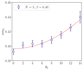
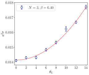
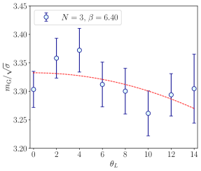
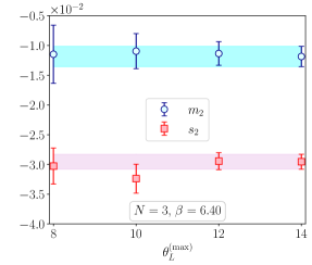
Figure 1: Results for $N=3$ with $\beta=6.40$. Examples of fits performed by using the functional form Eq. (18) for several quantities: (top left panel) the lightest glueball mass $am_{\mathrm{G}}$, (top right panel) the string tension $a^{2}\sigma$, (bottom left panel) the ratio $m_{\mathrm{G}}/\sqrt{\sigma}$. In the bottom right panel we show the dependence of the estimates of $m_{2}$ and $s_{2}$ on the upper limit of the fit range $\theta_{L}^{(\max)}$.

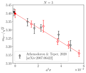
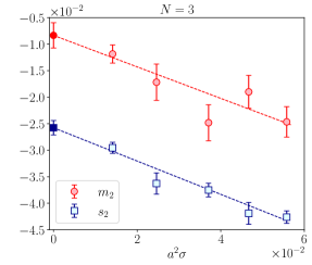
Figure 2: Left panel: continuum scaling of our $N=3$ results for $m_{0^{++}}/\sqrt{\sigma}$, compared with data reported in Ref. Athenodorou:2020ani . The dashed line is the result of a best fit of our data assuming $\mathcal{O}(a^{2})$ scaling corrections. Right panel: continuum scaling of our $N=3$ results for $m_{2}$ and $s_{2}$ and their continuum extrapolation assuming $\mathcal{O}(a^{2})$ scaling corrections.

The continuum extrapolations of $m_{2}$ and $s_{2}$ are displayed in Fig. 2. These results are obviously consistent with the presence of just the leading $\mathcal{O}(a^{2})$ finite-$a$ corrections. We thus obtain the continuum extrapolated values

$$m_{2}=-0.0083(23),\qquad\mathrm{(continuum\ extrapolated)},$$ (20)

$$s_{2}=-0.0258(14),\qquad\mathrm{(continuum\ extrapolated)}.$$ (21)

Remarkably, the continuum extrapolated value of $s_{2}$ is quite close to twice $m_{2}$, which means that the dimensionless ratio $m_{\mathrm{G}}(\theta)/\sqrt{\sigma(\theta)}$ is almost independent of $\theta$. If we define $g_{2}$ by the equation

$$\frac{m_{\mathrm{G}}(\theta)}{\sqrt{\sigma(\theta)}}=\frac{m_{0^{++}}}{\sqrt{\sigma}}[1+g_{2}\theta^{2}+\mathcal{O}(\theta^{4})],$$ (22)

we indeed have the continuum result:

$$g_{2}=m_{2}-\frac{s_{2}}{2}=0.0046(24),\qquad\mathrm{(continuum\ extrapolated)}.$$ (23)

That the ratio $m_{\mathrm{G}}(\theta)/\sqrt{\sigma(\theta)}$ is quite insensitive to the value of $\theta$ is also true at finite lattice spacing, as can be appreciated from the data reported in Tab. 1 and from the example displayed in Fig. 1.

Although we are not aware of any physical argument implying the vanishing of $g_{2}$, this result could suggest that all dimensionless quantities are independent of $\theta$. Such a strong statement can be however shown to be false. In Ref. DElia:2012pvq (see also DElia:2013uaf ; Bonanno:2023hhp ), the $\theta$-dependence of the $\mathrm{SU}(3)$ deconfinement critical temperature $T_{c}$ was studied, and it was concluded that

$$T_{c}(\theta)=T_{c}[1-R\theta^{2}+\mathcal{O}(\theta^{4})],$$ (24)

where $T_{c}$ is the $\theta=0$ critical temperature and

$$R=0.0178(5).$$ (25)

This can be recast in units of $\sqrt{\sigma(\theta)}$ as:

$$\frac{T_{c}(\theta)}{\sqrt{\sigma(\theta)}}=\frac{T_{c}}{\sqrt{\sigma}}[1-t_{2}\theta^{2}+\mathcal{O}(\theta^{4})],$$ (26)

with (using Eq. (21))

$$t_{2}=R+\frac{s_{2}}{2}=0.0049(9),$$ (27)

which is definitely different from zero.

3.2 Results for the $\mathrm{SU}(6)$ Yang–Mills theory

The general strategy adopted at $N=6$ is the same as for the case $N=3$. However, obtaining precise results in this case has proven to be a much more challenging task. We thus focused on just two values of the bare inverse lattice coupling, namely $\beta=25.056$ and $\beta=25.452$, corresponding to quite fine lattice spacings. Obviously, using estimates at only two values of the lattice spacing prevents us from performing a reliable continuum extrapolation in this case.

The use of the PTBC algorithm was instrumental in reducing the auto-correlation time of Monte Carlo simulations. In particular, for the two values of $\beta$ considered in this work, the PTBC algorithm allows to reduce the integrated auto-correlation time of the topological modes (at constant CPU time) by a factor of $\sim 20$ for $\beta=25.056$ Bonanno:2020hht , and by a factor of $\sim 60$ for $\beta=25.452$ Bonanno:2022yjr . In simulations performed at inverse coupling $\beta=25.056$ we produced and stored $\mathcal{O}(20\text{k})$ thermalized configurations at $\theta=0$ and $\mathcal{O}(13\text{k})$ configuration for each non-zero $\theta$ value, while for simulations at inverse coupling $\beta=25.452$ we produced and stored $\mathcal{O}(5\text{k})$ thermalized configurations for each non-zero value of $\theta$ (for $\theta=0$ we used results from a previous study, see Ref. Bonanno:2022yjr ). In all cases, measurements were performed every $10$ parallel tempering steps, using the same setup already adopted in Refs. Bonanno:2020hht ; Bonanno:2022yjr , to which we refer for more details.

Our results at $N=6$ for $m_{2}$ and $s_{2}$ are summarized in Tab. 2, while all raw data for $m_{\mathrm{G}}(\theta_{L})$ and $\sigma(\theta_{L})$ can be found in App. B. As it is clear from data in Tab. 2, and from the example shown in Fig. 3, the $\theta$ dependence of $m_{\mathrm{G}}(\theta)$ and $\sigma(\theta)$ is much milder at $N=6$ than it is at $N=3$. In particular, we can only provide upper bounds for $m_{2}$. This behavior is compatible with the expectation that $m_{2}$ and $s_{2}$ are suppressed in the large-$N$ limit.

The accuracy of the data collected at $N=6$ is not sufficient to directly test the expected DelDebbio:2006yuf $1/N^{2}$ behavior of $m_{2}$ and $s_{2}$. However, our data are definitely consistent with this scaling law, as can be appreciated from Fig. 4, where $N^{2}m_{2}$ and $N^{2}s_{2}$ are plotted together for $N=3$, $6$ as a function of $\sigma a^{2}$. To describe the large-$N$ behavior we can define the parameters $\bar{s}_{2}$ and $\bar{m}_{2}$ by:

$$s_{2}\simeq\bar{s}_{2}/N^{2}+\mathcal{O}(N^{-4})\ ,\quad m_{2}\simeq\bar{m}_{2}/N^{2}+\mathcal{O}(N^{-4})~{}.$$ (28)

Assuming the leading order large-$N$ scaling to be accurate already for $N\geq 3$, as is the case for other $\mathcal{O}(\theta^{2})$ quantities Bonanno:2020hht ; Bonanno:2023hhp , we can estimate these parameters using the results obtained for $N=3$:

$$\bar{s}_{2}\simeq-0.23(1)\ ,\quad\bar{m}_{2}\simeq-0.075(20)\ .$$ (29)

$L$	$\beta$	$Z_{Q}$	$am_{0^{++}}$	$m_{2}$	$a^{2}\sigma$	$s_{2}$
14	25.056	0.12053(88)*	0.7369(75)	-0.0004(55)	0.06278(27)	-0.0117(21)
16	25.452	0.13834(46)	0.6297(64)	-0.0088(64)	0.04467(25)	-0.0084(26)

Table 2: Summary of the results obtained for $N=6$. The value of $Z_{Q}$ denoted by an asterisk is from Ref. Bonanno:2020hht , while the value for $\beta=25.452$ has been computed anew in this work.

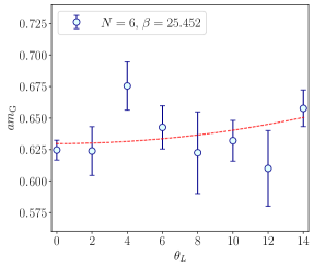
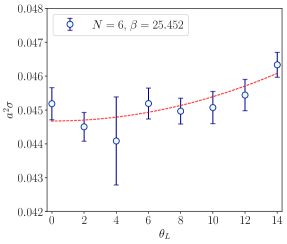
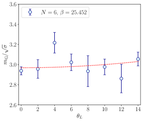
Figure 3: Results for $N=6$ with $\beta=25.452$. Examples of fits performed by using the functional form Eq. (18) for several quantities: (top left panel) the lightest glueball mass $am_{\mathrm{G}}$, (top right panel) the string tension $a^{2}\sigma$, (bottom panel) the ratio $m_{\mathrm{G}}/\sqrt{\sigma}$.

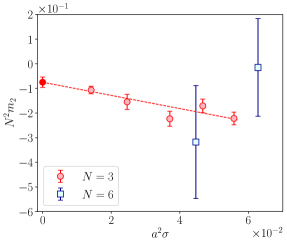
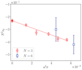
Figure 4: Continuum scaling of $N^{2}m_{2}$ and $N^{2}s_{2}$ for $N=3$ and $N=6$.

4 Conclusions

In this paper we presented a novel investigation of the $\theta$-dependence of the spectrum of four-dimensional $\mathrm{SU}(N)$ Yang–Mills theories. In particular, we focused on the leading order $\mathcal{O}(\theta^{2})$ dependence of the string tension $\sigma(\theta)$ and of the lightest glueball state $m_{\mathrm{G}}(\theta)$, and estimated the value of the parameters $s_{2}$ and $m_{2}$ defined in Eq. (3). The present study has been carried out by means of lattice simulations performed at imaginary values of the topological $\theta$-angle, using the so called analytic continuation approach. This approach proved to be extremely effective in reducing statistical uncertainties with respect to the previously adopted Taylor expansion method.

Our main results have been obtained for the $N=3$ theory, for which we were able to perform a controlled continuum extrapolation of $m_{2}$ and $s_{2}$, with the results:

$$m_{2}(N=3) = -0.0083(23),$$ (30)

$$s_{2}(N=3) = -0.0258(14).$$ (31)

The case $N=6$ was much more challenging, as expected a priori. Larger auto-correlation times make numerical simulations particularly demanding. Moreover, the values of $m_{2}$ and $s_{2}$ at $N=6$ are expected (by large-$N$ scaling) to be suppressed by a factor $\approx 4$ with respect to their value at $N=3$. To address the first problem we used the Parallel Tempering on Boundary Conditions algorithm, and yet the best we could do was to estimate the values of $m_{2}$ and $s_{2}$ for only two values of the lattice spacing, although two quite fine ones.

Due to the limited accuracy of the results at $N=6$, we cannot perform a stringent test of the expected $\mathcal{O}(N^{-2})$ behavior of $m_{2}$ and $s_{2}$. However, our data are definitely consistent with this expectation. Based on our previous experiences with $\mathcal{O}(\theta^{2})$ corrections (see, e.g., Refs. Bonanno:2020hht ; Bonanno:2023hhp ), it is natural to expect the large-$N$ scaling of $m_{2}$ and $s_{2}$ to be well approximated by the leading $\mathcal{O}(N^{-2})$ behavior already for $N=3$; using this assumption we get for the coefficients $\bar{s}_{2}$ and $\bar{m}_{2}$ defined in Eq. (28) the estimates

$$\bar{s}_{2}\simeq-0.23(1)\ ,\quad\bar{m}_{2}\simeq-0.075(20)\ .$$ (32)

As noted in the introduction, the parameters $m_{2}$ and $s_{2}$, which parameterize the leading order $\theta$-dependence of the spectrum, also parameterize the way in which the lightest glueball mass and the string tension are affected by the topological freezing, i.e., the systematics induced by using for their estimation an ensemble of gauge configurations with fixed topological charge. Such a quantitative information is very useful. Indeed, given the very fast growth of the integrated auto-correlation time of the topological charge as the continuum limit is approached, it is quite common to perform simulations at fixed $Q=0$ with large-$N$ gauge groups. Using our results in Eq. (32) and the general formula Eq. (5), it is possible to estimate the bias induced by using a fixed topological background. It turns out that already modestly large volumes are sufficient to have a negligible bias: considering for example the case $N=3$, in which case $\chi^{1/4}$ is roughly equal to $1\text{ fm}^{-1}$ (see, e.g., Bonanno:2023ple ), we have

$$\frac{\Delta m_{0^{++}}}{m_{0^{++}}}\Bigg{|}_{N=3}\approx\frac{m_{2}}{2\chi V}\approx-0.08\%$$ (33)

for $V\simeq(1.5\text{ fm})^{4}$. Using larger values of $N$ this estimate becomes drastically more favorable, since the topological susceptibility changes only slightly (see, e.g., Refs. Bonati:2016tvi ; Ce:2016awn ; Bonanno:2020hht ), while $m_{2}$ scales as $1/N^{2}$. These estimates constitute an independent confirmation of the results obtained in Ref. Bonanno:2022yjr , with the advantage of providing a quantitative upper bound to the accuracy that can be achieved when using simulations at fixed topological sector.

The results presented in this paper can be extended quite naturally in several different ways. One possibility is to accurately investigate $s_{2}$ and $m_{2}$ for $N>3$, in order to quantitatively asses the $N$ dependence of these coefficients. From the previous discussion it should be clear that this is not an easy task, and some ideas are required to further improve the signal-to-noise ratio. A second possibility is to study the excited glueball spectrum. In particular, it would be very interesting to understand (both theoretically and numerically) how the $\mathcal{O}(\theta^{2})$ correction to the mass depends on the state considered. Indeed, these corrections can not be all independent from each other, since they are indirectly related to the $\theta$-dependence of the free energy in the confined phase. This can be easily understood by using hadron resonance gas models like, e.g., those discussed in Caselle:2015tza ; Trotti:2022knd , where it was shown that a determination of the glueball masses is sufficient to obtain quantitatively accurate estimates of thermodynamical quantities. Finally, it would be very interesting to study models in which $s_{2}$ and $m_{2}$ or, more generally, the $\theta$-dependence of the spectrum, can be investigated analytically (and is non-trivial). Two-dimensional $\mathrm{CP}^{N-1}$ models are natural candidates.

Appendix

Appendix A Two-dimensional $\mathrm{U}(N)$ Yang–Mills theories

Two-dimensional Yang–Mills theories are particularly simple to investigate in the thermodynamic limit: neglecting boundary conditions, we can fix $U_{1}(x)=1$ on all the sites and $U_{2}(x)=1$ along a single line at constant $x_{1}$. In this way it is simple to show, using the invariance properties of the Haar measure, that link integrals can be traded for plaquette integrals and the theory reduces to a single-plaquette model Gross:1980he .

Using for the topological charge density the definition Bonati:2019ylr

$$q(x)=\frac{1}{2\pi}\mathrm{arg}\det(\Pi_{12}(x))\ ,$$ (34)

where $\Pi_{12}(x)$ denotes the plaquette in position $x$, the string tension at inverse ’t Hooft lattice coupling $\lambda=\beta/(2N^{2})$ can be written as Gross:1980he

$$\sigma(N,\lambda,\theta) =-\log\left(\frac{1}{Z_{1p}(N,\lambda,\theta)}\int\mathrm{d}W\frac{1}{N}\mathrm{tr}(W)e^{N\lambda\mathrm{tr}(W+W^{{\dagger}})+\frac{\theta}{2\pi}\mathrm{tr}\log(W)}\right)$$ (35)

$$=-\log\left(\frac{1}{2N^{2}}\frac{\mathrm{d}}{\mathrm{d}\lambda}\log Z_{1p}(N,\lambda,\theta)\right)\ ,$$

where $\mathrm{d}W$ is the Haar measure on U($N$) and

$$Z_{1p}(N,\lambda,\theta)=\int\mathrm{d}We^{N\lambda\mathrm{tr}(W+W^{{\dagger}})+\frac{\theta}{2\pi}\mathrm{tr}\log(W)}\ .$$ (36)

It is also simple to show that the connected correlator of two plaquette identically vanishes whenever the two plaquettes are not coincident, hence no finite glueball mass can be defined.

Using the Weyl form of the Haar measure for class functions, it is possible to rewrite, using manipulations completely analogous to those used in Gross:1980he ; Bars:1979xb , the single-plaquette partition function as a $N\times N$ determinant Bonati:2019ylr

$$Z_{1p}(N,\lambda,\theta)=\det\left(\mathcal{I}_{i-j+\frac{\theta}{2\pi}}(2N\lambda)\right)\ ,\quad i,j=1,\ldots N\ ,$$ (37)

where the functions $\mathcal{I}_{\nu}(x)$ are defined by

$$\mathcal{I}_{\nu}(x)=\frac{1}{2\pi}\int_{-\pi}^{\pi}e^{i\nu\phi}e^{x\cos\phi}\mathrm{d}\phi\ .$$ (38)

We thus have (for $k,j=1,\ldots,N$)

$$Z_{1p}(N,\lambda,\theta)=\int\mathrm{det}\left[e^{i\phi_{j}(k-j)}\right]e^{i\frac{\theta}{2\pi}\sum_{j}\phi_{j}}e^{2N\lambda\sum_{j}\cos\phi_{j}}\prod\frac{\mathrm{d}\phi_{j}}{2\pi}\ ,$$ (39)

and to study the leading behavior in the limit $\lambda\to\infty$ it is sufficient to replace $\cos\phi_{j}$ by $1-\frac{1}{2}\phi_{j}^{2}$ in the exponentials, obtaining

$$Z_{1p}(N,\lambda\gg 1,\theta)=\left(\frac{e^{2\lambda N}}{\sqrt{4\pi\lambda N}}\right)^{N}\det\left[e^{-\frac{1}{4N\lambda}\left(k-j+\frac{\theta}{2\pi}\right)^{2}}\right]\ .$$ (40)

By using the multi-linearity of the determinant we can rewrite this expression as follows

$$Z_{1p}(N,\lambda\gg 1,\theta) =\left(\frac{e^{2\lambda N}}{\sqrt{4\pi\lambda N}}\right)^{N}\det\left[e^{-\frac{1}{4N\lambda}\left(k-j\right)^{2}}\right]\exp\left\{-\frac{1}{4\lambda}\left(\frac{\theta}{2\pi}\right)^{2}\right\}=$$ (41)

$$=Z_{1p}(N,\lambda\gg 1,\theta=0)\exp\left\{-\frac{1}{4\lambda}\left(\frac{\theta}{2\pi}\right)^{2}\right\}\ ,$$

where

$$Z_{1p}(N,\lambda\gg 1,\theta=0)=\left(\frac{e^{2\lambda N}}{\sqrt{4\pi\lambda N}}\right)^{N}e^{-\frac{1}{2\lambda N}\sum_{k=1}^{N}k^{2}}\det\left[e^{-\frac{jk}{2N\lambda}}\right]\ ,$$ (42)

and the remaining determinant can be related to a Vandermonde determinant. Using these expressions in Eq. (35) we see that for $\lambda\gg 1$ we have

$$\frac{\mathrm{d}}{\mathrm{d}\lambda}\log Z_{1p}(N,\lambda\gg 1,\theta=0)=2N^{2}-\frac{N}{2\lambda}+o(\lambda^{-1})\ ,$$ (43)

and to reliably estimate subleading terms we should go beyond the leading order expansion of Eq. (37). The $\theta\neq 0$ contribution is the subleading $N$-independent correction $\frac{\theta^{2}}{16\pi^{2}\lambda^{2}}$, hence the continuum string tension does not depend on $\theta$.

Appendix B Raw data for four-dimensional $\mathrm{SU}(3)$ and $\mathrm{SU}(6)$ Yang–Mills theories

In this appendix we collect all the results obtained for $am_{\mathrm{G}}(\theta_{L})$ and $a^{2}\sigma(\theta_{L})$ at the different values of the inverse lattice coupling $\beta$ for $N=3$ (Tab. 3) and $N=6$ (Tab. 4).

$L$	$\beta$	$\theta_{L}$	$am_{\mathrm{G}}$	$a^{2}\sigma$
16	5.95	0	0.7487(62)	0.05576(19)
		2	0.7409(15)	0.05478(43)
		4	0.7560(15)	0.05652(23)
		6	0.7473(14)	0.05718(20)
		8	0.7589(72)	0.05816(45)
		10	0.804(16)	0.05961(23)
		12	0.7892(71)	0.06097(22)
		14	0.7922(77)	0.06283(24)
		16	0.8231(76)	0.06515(26)

$L$	$\beta$	$\theta_{L}$	$am_{\mathrm{G}}$	$a^{2}\sigma$
18	6.00	0	0.6865(61)	0.04659(31)
		5	0.7008(65)	0.04757(17)
		8	0.744(12)	0.04930(19)
		10	0.7190(67)	0.05014(19)
		12	0.7301(62)	0.05155(21)
		14	0.7364(64)	0.05475(46)

$L$	$\beta$	$\theta_{L}$	$am_{\mathrm{G}}$	$a^{2}\sigma$
18	6.07	0	0.6261(45)	0.03710(11)
		5	0.6296(55)	0.03787(14)
		8	0.6417(55)	0.03898(24)
		10	0.6495(57)	0.04027(14)
		12	0.676(11)	0.04149(15)
		14	0.707(11)	0.04357(28)

$L$	$\beta$	$\theta_{L}$	$am_{\mathrm{G}}$	$a^{2}\sigma$
22	6.20	0	0.5187(78)	0.02425(23)
		5	0.5312(78)	0.02543(15)
		8	0.5410(85)	0.02653(10)
		10	0.5482(83)	0.02760(29)
		12	0.5576(92)	0.02839(30)
		14	0.5792(98)	0.03036(20)

$L$	$\beta$	$\theta_{L}$	$am_{\mathrm{G}}$	$a^{2}\sigma$
30	6.40	0	0.3923(36)	0.014104(80)
		2	0.4014(40)	0.014297(87)
		4	0.4033(44)	0.014304(93)
		6	0.4033(46)	0.014837(97)
		8	0.4084(48)	0.015314(97)
		10	0.4154(46)	0.01622(16)
		12	0.4254(47)	0.016680(83)
		14	0.4397(79)	0.01770(13)

Table 3: Summary of all obtained results for $N=3$.

$L$	$\beta$	$\theta_{L}$	$am_{\mathrm{G}}$	$a^{2}\sigma$
14	25.056	0	0.748(11)	0.06137(77)
		2	0.757(27)	0.06351(44)
		4	0.761(27)	0.06307(44)
		6	0.717(15)	0.06261(97)
		8	0.725(13)	0.06241(99)
		10	0.679(25)	0.06256(95)
		12	0.811(31)	0.06426(50)
		14	0.742(13)	0.06559(47)
		16	0.735(16)	0.06530(45)

$L$	$\beta$	$\theta_{L}$	$am_{\mathrm{G}}$	$a^{2}\sigma$
16	25.452	0	0.6246(78)	0.04518(48)
		2	0.624(19)	0.04450(43)
		4	0.676(19)	0.0441(13)
		6	0.643(17)	0.04519(46)
		8	0.622(32)	0.04496(38)
		10	0.632(16)	0.04507(48)
		12	0.610(30)	0.04544(46)
		14	0.658(15)	0.04633(37)

Table 4: Summary of all obtained results for $N=6$.

References

- (1) S. Coleman, Aspects of Symmetry: Selected Erice Lectures. Cambridge University Press, Cambridge, U.K., 1985.
- (2) R. Jackiw, Introduction to the Yang-Mills Quantum Theory, Rev. Mod. Phys. 52 (1980) 661.
- (3) D. J. Gross, R. D. Pisarski and L. G. Yaffe, QCD and Instantons at Finite Temperature, Rev. Mod. Phys. 53 (1981) 43.
- (4) T. Schäfer and E. V. Shuryak, Instantons in QCD, Rev. Mod. Phys. 70 (1998) 323 [hep-ph/9610451].
- (5) A. D’Adda, M. Lüscher and P. Di Vecchia, A Expandable Series of Nonlinear Sigma Models with Instantons, Nucl. Phys. B 146 (1978) 63.
- (6) E. Witten, Instantons, the Quark Model, and the Expansion, Nucl. Phys. B 149 (1979) 285.
- (7) T. G. Kovacs, E. T. Tomboulis and Z. Schram, Topology on the lattice: 2-d Yang-Mills theories with a theta term, Nucl. Phys. B 454 (1995) 45 [hep-th/9505005].
- (8) C. Bonati and P. Rossi, Topological susceptibility of two-dimensional gauge theories, Phys. Rev. D 99 (2019) 054503 [1901.09830].
- (9) C. Bonati and P. Rossi, Topological effects in continuum two-dimensional gauge theories, Phys. Rev. D 100 (2019) 054502 [1908.07476].
- (10) D. Gaiotto, A. Kapustin, Z. Komargodski and N. Seiberg, Theta, Time Reversal, and Temperature, JHEP 05 (2017) 091 [1703.00501].
- (11) C. Bonati and M. D’Elia, Topological critical slowing down: variations on a toy model, Phys. Rev. E 98 (2018) 013308 [1709.10034].
- (12) P. Di Vecchia and G. Veneziano, Chiral Dynamics in the Large Limit, Nucl. Phys. B 171 (1980) 253.
- (13) G. Grilli di Cortona, E. Hardy, J. Pardo Vega and G. Villadoro, The QCD axion, precisely, JHEP 01 (2016) 034 [1511.02867].
- (14) A. Boccaletti and D. Nogradi, The semi-classical approximation at high temperature revisited, JHEP 03 (2020) 045 [2001.03383].
- (15) C. Bonati, M. D’Elia, M. Mariti, G. Martinelli, M. Mesiti, F. Negro et al., Axion phenomenology and -dependence from lattice QCD, JHEP 03 (2016) 155 [1512.06746].
- (16) P. Petreczky, H.-P. Schadler and S. Sharma, The topological susceptibility in finite temperature QCD and axion cosmology, Phys. Lett. B 762 (2016) 498 [1606.03145].
- (17) J. Frison, R. Kitano, H. Matsufuru, S. Mori and N. Yamada, Topological susceptibility at high temperature on the lattice, JHEP 09 (2016) 021 [1606.07175].
- (18) S. Borsanyi et al., Calculation of the axion mass based on high-temperature lattice quantum chromodynamics, Nature 539 (2016) 69 [1606.07494].
- (19) C. Bonati, M. D’Elia, G. Martinelli, F. Negro, F. Sanfilippo and A. Todaro, Topology in full QCD at high temperature: a multicanonical approach, JHEP 11 (2018) 170 [1807.07954].
- (20) F. Burger, E.-M. Ilgenfritz, M. P. Lombardo and A. Trunin, Chiral observables and topology in hot QCD with two families of quarks, Phys. Rev. D 98 (2018) 094501 [1805.06001].
- (21) TWQCD collaboration, Y.-C. Chen, T.-W. Chiu and T.-H. Hsieh, Topological susceptibility in finite temperature QCD with physical (u/d,s,c) domain-wall quarks, Phys. Rev. D 106 (2022) 074501 [2204.01556].
- (22) A. Athenodorou, C. Bonanno, C. Bonati, G. Clemente, F. D’Angelo, M. D’Elia et al., Topological susceptibility of Nf = 2 + 1 QCD from staggered fermions spectral projectors at high temperatures, JHEP 10 (2022) 197 [2208.08921].
- (23) B. Alles, M. D’Elia and A. Di Giacomo, Topological susceptibility at zero and finite T in SU(3) Yang-Mills theory, Nucl. Phys. B 494 (1997) 281 [hep-lat/9605013].
- (24) B. Alles, M. D’Elia and A. Di Giacomo, Topology at zero and finite in Yang–Mills theory, Phys. Lett. B 412 (1997) 119 [hep-lat/9706016].
- (25) L. Del Debbio, L. Giusti and C. Pica, Topological susceptibility in the gauge theory, Phys. Rev. Lett. 94 (2005) 032003 [hep-th/0407052].
- (26) L. Del Debbio, H. Panagopoulos and E. Vicari, dependence of gauge theories, JHEP 08 (2002) 044 [hep-th/0204125].
- (27) M. D’Elia, Field theoretical approach to the study of theta dependence in Yang-Mills theories on the lattice, Nucl. Phys. B 661 (2003) 139 [hep-lat/0302007].
- (28) B. Lucini, M. Teper and U. Wenger, Topology of gauge theories at and , Nucl. Phys. B 715 (2005) 461 [hep-lat/0401028].
- (29) L. Giusti, S. Petrarca and B. Taglienti, dependence of the vacuum energy in the gauge theory from the lattice, Phys. Rev. D 76 (2007) 094510 [0705.2352].
- (30) E. Vicari and H. Panagopoulos, dependence of gauge theories in the presence of a topological term, Phys. Rept. 470 (2009) 93 [0803.1593].
- (31) H. Panagopoulos and E. Vicari, The gauge theory with an imaginary term, JHEP 11 (2011) 119 [1109.6815].
- (32) C. Bonati, M. D’Elia, H. Panagopoulos and E. Vicari, Change of Dependence in Gauge Theories Across the Deconfinement Transition, Phys. Rev. Lett. 110 (2013) 252003 [1301.7640].
- (33) M. Cè, C. Consonni, G. P. Engel and L. Giusti, Non-Gaussianities in the topological charge distribution of the Yang–Mills theory, Phys. Rev. D 92 (2015) 074502 [1506.06052].
- (34) M. Cè, M. Garcia Vera, L. Giusti and S. Schaefer, The topological susceptibility in the large- limit of SU() Yang-Mills theory, Phys. Lett. B 762 (2016) 232 [1607.05939].
- (35) E. Berkowitz, M. I. Buchoff and E. Rinaldi, Lattice QCD input for axion cosmology, Phys. Rev. D 92 (2015) 034507 [1505.07455].
- (36) S. Borsanyi, M. Dierigl, Z. Fodor, S. Katz, S. Mages, D. Nogradi et al., Axion cosmology, lattice QCD and the dilute instanton gas, Phys. Lett. B 752 (2016) 175 [1508.06917].
- (37) C. Bonati, M. D’Elia and A. Scapellato, dependence in Yang-Mills theory from analytic continuation, Phys. Rev. D 93 (2016) 025028 [1512.01544].
- (38) C. Bonati, M. D’Elia, P. Rossi and E. Vicari, dependence of 4D gauge theories in the large- limit, Phys. Rev. D 94 (2016) 085017 [1607.06360].
- (39) C. Bonati, M. Cardinali and M. D’Elia, dependence in trace deformed Yang-Mills theory: a lattice study, Phys. Rev. D 98 (2018) 054508 [1807.06558].
- (40) C. Bonati, M. Cardinali, M. D’Elia and F. Mazziotti, -dependence and center symmetry in Yang-Mills theories, Phys. Rev. D 101 (2020) 034508 [1912.02662].
- (41) E. Witten, Current Algebra Theorems for the Goldstone Boson, Nucl. Phys. B 156 (1979) 269.
- (42) G. Veneziano, Without Instantons, Nucl. Phys. B 159 (1979) 213.
- (43) E. Witten, Large Chiral Dynamics, Annals Phys. 128 (1980) 363.
- (44) M. Campostrini and P. Rossi, expansion of the topological susceptibility in the models, Phys. Lett. B 272 (1991) 305.
- (45) L. Del Debbio, G. M. Manca, H. Panagopoulos, A. Skouroupathis and E. Vicari, -dependence of the spectrum of gauge theories, JHEP 06 (2006) 005 [hep-th/0603041].
- (46) P. Rossi, Effective Lagrangian of models in the large limit, Phys. Rev. D D94 (2016) 045013 [1606.07252].
- (47) E. Vicari, Monte Carlo simulation of lattice models at large , Phys. Lett. B 309 (1993) 139 [hep-lat/9209025].
- (48) C. Bonanno, C. Bonati and M. D’Elia, Topological properties of models in the large- limit, JHEP 01 (2019) 003 [1807.11357].
- (49) M. Berni, C. Bonanno and M. D’Elia, Large- expansion and -dependence of models beyond the leading order, Phys. Rev. D 100 (2019) 114509 [1911.03384].
- (50) B. Lucini, M. Teper and U. Wenger, Glueballs and -strings in gauge theories: Calculations with improved operators, JHEP 06 (2004) 012 [hep-lat/0404008].
- (51) A. Athenodorou and M. Teper, The glueball spectrum of SU(3) gauge theory in 3 + 1 dimensions, JHEP 11 (2020) 172 [2007.06422].
- (52) A. Athenodorou and M. Teper, SU(N) gauge theories in 3+1 dimensions: glueball spectrum, string tensions and topology, JHEP 12 (2021) 082 [2106.00364].
- (53) D. Vadacchino, A review on Glueball hunting, 2305.04869.
- (54) B. Alles, G. Boyd, M. D’Elia, A. Di Giacomo and E. Vicari, Hybrid Monte Carlo and topological modes of full QCD, Phys. Lett. B 389 (1996) 107 [hep-lat/9607049].
- (55) L. Del Debbio, G. M. Manca and E. Vicari, Critical slowing down of topological modes, Phys. Lett. B 594 (2004) 315 [hep-lat/0403001].
- (56) ALPHA collaboration, S. Schaefer, R. Sommer and F. Virotta, Critical slowing down and error analysis in lattice QCD simulations, Nucl. Phys. B 845 (2011) 93 [1009.5228].
- (57) M. Hasenbusch, Fighting topological freezing in the two-dimensional model, Phys. Rev. D 96 (2017) 054504 [1706.04443].
- (58) C. Bonanno, C. Bonati and M. D’Elia, Large- Yang-Mills theories with milder topological freezing, JHEP 03 (2021) 111 [2012.14000].
- (59) R. Brower, S. Chandrasekharan, J. W. Negele and U. J. Wiese, QCD at fixed topology, Phys. Lett. B 560 (2003) 64 [hep-lat/0302005].
- (60) S. Aoki, H. Fukaya, S. Hashimoto and T. Onogi, Finite volume QCD at fixed topological charge, Phys. Rev. D 76 (2007) 054508 [0707.0396].
- (61) M. Campostrini, A. Di Giacomo and H. Panagopoulos, The Topological Susceptibility on the Lattice, Phys. Lett. B 212 (1988) 206.
- (62) B. Berg, Dislocations and Topological Background in the Lattice Model, Phys. Lett. B 104 (1981) 475.
- (63) Y. Iwasaki and T. Yoshie, Instantons and Topological Charge in Lattice Gauge Theory, Phys. Lett. B 131 (1983) 159.
- (64) S. Itoh, Y. Iwasaki and T. Yoshie, Stability of Instantons on the Lattice and the Renormalized Trajectory, Phys. Lett. B 147 (1984) 141.
- (65) M. Teper, Instantons in the Quantized Vacuum: A Lattice Monte Carlo Investigation, Phys. Lett. B 162 (1985) 357.
- (66) E.-M. Ilgenfritz, M. Laursen, G. Schierholz, M. Müller-Preussker and H. Schiller, First Evidence for the Existence of Instantons in the Quantized Lattice Vacuum, Nucl. Phys. B 268 (1986) 693.
- (67) APE collaboration, M. Albanese et al., Glueball Masses and String Tension in Lattice QCD, Phys. Lett. B 192 (1987) 163.
- (68) M. Campostrini, A. Di Giacomo, H. Panagopoulos and E. Vicari, Topological Charge, Renormalization and Cooling on the Lattice, Nucl. Phys. B 329 (1990) 683.
- (69) B. Alles, L. Cosmai, M. D’Elia and A. Papa, Topology in models on the lattice: A Critical comparison of different cooling techniques, Phys. Rev. D 62 (2000) 094507 [hep-lat/0001027].
- (70) C. Morningstar and M. J. Peardon, Analytic smearing of SU(3) link variables in lattice QCD, Phys. Rev. D 69 (2004) 054501 [hep-lat/0311018].
- (71) M. Lüscher, Trivializing maps, the Wilson flow and the HMC algorithm, Commun. Math. Phys. 293 (2010) 899 [0907.5491].
- (72) M. Lüscher, Properties and uses of the Wilson flow in lattice QCD, JHEP 08 (2010) 071 [1006.4518].
- (73) C. Bonati and M. D’Elia, Comparison of the gradient flow with cooling in pure gauge theory, Phys. Rev. D D89 (2014) 105005 [1401.2441].
- (74) C. Alexandrou, A. Athenodorou and K. Jansen, Topological charge using cooling and the gradient flow, Phys. Rev. D 92 (2015) 125014 [1509.04259].
- (75) G. Bhanot and F. David, The Phases of the Model for Imaginary , Nucl. Phys. B 251 (1985) 127.
- (76) V. Azcoiti, G. Di Carlo, A. Galante and V. Laliena, New proposal for numerical simulations of theta vacuum - like systems, Phys. Rev. Lett. 89 (2002) 141601 [hep-lat/0203017].
- (77) B. Alles and A. Papa, Mass gap in the non-linear sigma model with a term, Phys. Rev. D 77 (2008) 056008 [0711.1496].
- (78) M. Imachi, M. Kambayashi, Y. Shinno and H. Yoneyama, The -term, model and the inversion approach in the imaginary- method, Prog. Theor. Phys. 116 (2006) 181.
- (79) S. Aoki, R. Horsley, T. Izubuchi, Y. Nakamura, D. Pleiter, P. E. L. Rakow et al., The Electric dipole moment of the nucleon from simulations at imaginary vacuum angle theta, 0808.1428.
- (80) B. Alles, M. Giordano and A. Papa, Behavior near of the mass gap in the two-dimensional non-linear sigma model, Phys. Rev. B 90 (2014) 184421 [1409.1704].
- (81) M. D’Elia and F. Negro, dependence of the deconfinement temperature in Yang–Mills theories, Phys. Rev. Lett. 109 (2012) 072001 [1205.0538].
- (82) M. D’Elia and F. Negro, Phase diagram of Yang-Mills theories in the presence of a term, Phys. Rev. D 88 (2013) 034503 [1306.2919].
- (83) C. Bonanno, M. D’Elia and L. Verzichelli, The -dependence of the critical temperature at large , 2312.12202.
- (84) M. Creutz, Overrelaxation and Monte Carlo Simulation, Phys. Rev. D 36 (1987) 515.
- (85) M. Creutz, Monte Carlo Study of Quantized Gauge Theory, Phys. Rev. D 21 (1980) 2308.
- (86) A. D. Kennedy and B. J. Pendleton, Improved Heat Bath Method for Monte Carlo Calculations in Lattice Gauge Theories, Phys. Lett. B 156 (1985) 393.
- (87) C. Bonanno, Lattice determination of the topological susceptibility slope of CPN-1 models at large , Phys. Rev. D 107 (2023) 014514 [2212.02330].
- (88) C. Bonanno, M. D’Elia, B. Lucini and D. Vadacchino, Towards glueball masses of large-N SU(N) pure-gauge theories without topological freezing, Phys. Lett. B 833 (2022) 137281 [2205.06190].
- (89) J. L. Dasilva Golán, C. Bonanno, M. D’Elia, M. García Pérez and A. Giorgieri, The twisted gradient flow strong coupling with parallel tempering on boundary conditions, PoS LATTICE2023 (2024) 354 [2312.09212].
- (90) M. Lüscher and S. Schaefer, Lattice QCD without topology barriers, JHEP 07 (2011) 036 [1105.4749].
- (91) B. Berg and A. Billoire, Glueball spectroscopy in su() lattice gauge theory (i), Nuclear Physics B 221 (1983) 109.
- (92) M. Teper, An improved method for lattice glueball calculations, Physics Letters B 183 (1987) 345.
- (93) M. J. Teper, SU() gauge theories in -dimensions, Phys. Rev. D 59 (1999) 014512 [hep-lat/9804008].
- (94) B. Lucini and M. Teper, gauge theories in four-dimensions: Exploring the approach to , JHEP 06 (2001) 050 [hep-lat/0103027].
- (95) B. Blossier, M. Della Morte, G. von Hippel, T. Mendes and R. Sommer, On the generalized eigenvalue method for energies and matrix elements in lattice field theory, JHEP 04 (2009) 094 [0902.1265].
- (96) B. Lucini, A. Rago and E. Rinaldi, Glueball masses in the large- limit, JHEP 08 (2010) 119 [1007.3879].
- (97) E. Bennett, J. Holligan, D. K. Hong, J.-W. Lee, C. J. D. Lin, B. Lucini et al., Glueballs and strings in Yang-Mills theories, Phys. Rev. D 103 (2021) 054509 [2010.15781].
- (98) P. de Forcrand, G. Schierholz, H. Schneider and M. Teper, The String and Its Tension in SU(3) Lattice Gauge Theory: Towards Definitive Results, Phys. Lett. B 160 (1985) 137.
- (99) C. Bonanno, The topological susceptibility slope of the pure-gauge Yang–Mills theory, JHEP 01 (2024) 116 [2311.06646].
- (100) M. Caselle, A. Nada and M. Panero, Hagedorn spectrum and thermodynamics of SU(2) and SU(3) Yang-Mills theories, JHEP 07 (2015) 143 [1505.01106].
- (101) E. Trotti, S. Jafarzade and F. Giacosa, Thermodynamics of the glueball resonance gas, Eur. Phys. J. C 83 (2023) 390 [2212.03272].
- (102) D. J. Gross and E. Witten, Possible Third Order Phase Transition in the Large N Lattice Gauge Theory, Phys. Rev. D 21 (1980) 446.
- (103) I. Bars and F. Green, Complete Integration of U () Lattice Gauge Theory in a Large Limit, Phys. Rev. D 20 (1979) 3311.