Mixed Noise and Posterior Estimation with Conditional DeepGEM

Abstract

Motivated by indirect measurements and applications from nanometrology with a mixed noise model, we develop a novel algorithm for jointly estimating the posterior and the noise parameters in Bayesian inverse problems. We propose to solve the problem by an expectation maximization (EM) algorithm. Based on the current noise parameters, we learn in the E-step a conditional normalizing flow that approximates the posterior. In the M-step, we propose to find the noise parameter updates again by an EM algorithm, which has analytical formulas. We compare the training of the conditional normalizing flow with the forward and reverse KL, and show that our model is able to incorporate information from many measurements, unlike previous approaches.

1 Introduction

In numerous healthcare and other contemporary applications, the variables of primary interest are obtained through indirect measurements, such as in the case of Magnetic Resonance Imaging (MRI) and Computed Tomography (CT). For some of these applications, the reliability of the results is of particular importance. The accuracy and trustworthiness of the outcomes obtained through indirect measurements are significantly influenced by two critical factors: the degree of uncertainty associated with the measuring instrument and the appropriateness of the (forward) model used for the reconstruction of the parameters of interest (measurand). In this paper, we consider Bayesian inversion to obtain the measurand from signals measured by the instrument and a noise model that mimics both the instrument noise and the error of the forward model. Within this framework, we developed an extension of the expectation maximization (EM) algorithm that is able to handle a Bayesian inversion with a measurement noise model. As a result, we obtain the posterior distribution for the parameters of interest (distribution of the measurand), which is a measure of the reliability of the measurement results. To demonstrate the applicability and effectiveness we apply the algorithm to two real examples in nanometrology, i.e. EUV Scatteroemtry. The key focus of the work is the development of a noise-adapted posterior sampler based on DeepGEM [21], which can incorporate information from several measurements simultaneously.

In this context we consider Bayesian inverse problems

$$Y_{\theta}=F(X)+\eta_{\theta},$$ (1)

with a possibly nonlinear forward operator $F\colon\mathbb{R}^{d}\to\mathbb{R}^{n}$ and a random noise variable $\eta_{\theta}$ which depends on an unknown parameter $\theta$ and on $F(X)$. Note, $Y$ describes the signals of the instrument whereas $X$ are the parameters of interest. The posterior (parameter distribution) $P_{X|Y_{\theta}=y}$ for observations $y$ will ultimately depend on these parameters $\theta$, as the likelihood $P_{Y_{\theta}|X=x}$ depends on them. Therefore, we aim to estimate the parameter $\theta$ from observations $y_{i}$, $i=1,...,N$, where $N$ is possibly small. There exists plenty of literature on estimating the standard deviation $\sigma$ within the Gaussian noise model $\eta_{\theta}=\eta_{\sigma}\sim\mathcal{N}(0,\sigma^{2}I_{n})$. However, motivated by applications in nanometrology [27], we are interested in a mixture of additive and multiplicative Gaussian noise of the form

$$\eta_{\theta}=\eta_{(a,b)}=\eta_{1}+\eta_{2},\quad\eta_{1}\sim\mathcal{N}(0,a^{2}),\;\eta_{2}\sim\mathcal{N}\big{(}0,b^{2}\text{diag}(F(x)^{2})\big{)},$$ (2)

where $F(x)=(F_{i}(x))_{i=1}^{n}$. For convenience we assume that the instrument noise as well as the model error can be described by the simple Ansatz made here. In general different noise models may appear in the applications. The noise model Eq.(2) was used in several previous studies in optics [26, 27, 28, 52] and analyzed in [18]. A similar noise model appears in analytical chemistry [51] and the study of gene expression arrays [50].

The standard approach for parameter estimation is maximum likelihood estimation. That is, we choose $\theta$ as the minimizer of the negative log likelihood function

$$\mathcal{L}(\theta)=\frac{1}{N}\sum_{i=1}^{N}\log(p_{\theta}(y_{i})),$$

where $p_{\theta}$ is the probability density function of $Y_{\theta}$. However, in our case this function involves a high-dimensional integral of the form $\int_{x}p_{Y_{\theta}|X=x}(y)dP_{X}(x)$ which is intractable to compute. As a remedy, we exploit expectation maximization (EM) algorithms which were introduced in [15], see also [9] for an overview and [45, 46] for applications for parameter estimation in inverse problems. The basic idea is to iteratively compute the posterior distribution $P_{X|Y_{\theta^{(r)}}=y_{i}}$ for a current estimate $\theta^{(r)}$ of $\theta$ and then updating this estimate to $\theta^{(r+1)}$ based on this posterior distribution. Here, the computation of $P_{X|Y_{\theta^{(r)}}=y_{i}}$ is called E-step, while the update of $\theta$ is called M-step. Intuitively, this corresponds to the idea that the distribution of $F(X)$ is approximately concentrated on a lower-dimensional manifold and consequently the distance of the $y_{i}$ to this manifold contains the information of the noise parameters $\theta$.

Recently, Gao et al. [21] proposed to solve the E-step by a normalizing flow (NF) [17] using the reverse/backward Kullback-Leibler (KL) divergence as loss function. For the M-step, they apply a stochastic gradient ascent algorithm. Note that in general the same procedure can be applied to estimate parameters of the forward operator instead of the noise level, see [37]. This approach has several drawbacks. The model needs to be retrained for every new observations $y$ and cannot profit from many observations that follow the same error parameters. Furthermore, the reverse KL is known to be mode-seeking. That is, it tends to recover only one mode of multimodal distributions, which incorporates a significant approximation error, see the discussions in [23, 43, 60] for more details.

Contributions

First, we propose to use the NF conditional normalizing flows [6, 59] in the E-step. This allows the incorporation of several measurements from the same error model and to solve the inverse problem for all measurements simultaneously. Fortunately, the forward KL can be used as loss function for training the conditional NFs which makes the method mode seeking. Second, we propose an inner EM algorithm for solving the M-step more efficiently. For our special noise model (2), we deduce analytic expressions for E- and M-steps of this inner algorithm. The performance of our approach will be demonstrated on two applications from nanooptics. In particular, we we propose a conditional version of DeepGEM and benchmark it against forward conditional DeepGEM, where the reverse KL is replaced by a forward KL.

Organization

We start in Section 2 by recalling the general EM algorithm. Then, in Section 3, we construct the E- and M-step for our application. That is, we show how conditional normalizing flows can be incorporated into the E-step and describe how the M-step can be solved for our noise model with an “inner” EM algorithm which steps can given in a closed analytical form. Some of the technical computations are postponed to Appendix A. We test our algorithms on two nanooptics problems, which is done in section 4. Finally, conclusions are drawn in Section 5.

2 EM Algorithm

In this section, we introduce the EM algorithm as a maximization-maximization algorithm of an evidence lower bound. A general introduction into the EM algorithm can be found, e.g., in [9].

Let $\{Y_{\theta}\mathrel{\mathop{\ordinarycolon}}\theta\in\Theta\}$ be a family of $n$-dimensional random variables having probability density functions $p_{\theta}$, $\theta\in\Theta$. Given i.i.d. samples $y_{1},...,y_{N}\in\mathbb{R}^{n}$ from $Y_{\theta^{*}}$ for some unknown $\theta^{*}$, we want approximate $\theta^{*}$ by computing the maximum log-likelihood estimator

$$\hat{\theta}=\operatorname*{arg\,max}_{\theta\in\Theta}\mathcal{L}(\theta),\quad\mathcal{L}(\theta)\coloneqq\frac{1}{N}\sum_{i=1}^{N}\log(p_{\theta}(y_{i})).$$

In the literature, the term $\log(p_{\theta}(y))$ is also called evidence of $y$ under $\theta$. As in many applications it is hard to maximize $\mathcal{L}$, we introduce an absolute continuous $d$-dimensional auxiliary random variable $X$ such that the joint density $p_{X,Y_{\theta}}$ exists and is easy to evaluate. Then, it holds by the law of total probability and Jensen’s inequality, for any probability density function $q$ on $\mathbb{R}^{d}$, that

$$\log(p_{\theta}(y)) =\log\Big{(}\int_{\mathbb{R}^{d}}p_{X,Y_{\theta}}(x,y)\mathrm{d}x\Big{)}=\log\Big{(}\int_{\mathbb{R}^{d}}\frac{p_{X,Y_{\theta}}(x,y)}{q(x)}q(x)\mathrm{d}x\Big{)}$$ (3)

$$\geq\int_{\mathbb{R}^{d}}\log\Big{(}\frac{p_{X,Y_{\theta}}(x,y)}{q(x)}\Big{)}q(x)\mathrm{d}x\eqqcolon\mathcal{F}(q,\theta|y).$$ (4)

We call the random variable $X$ the hidden variable and the expression $\mathcal{F}(q,\theta|y)$ the evidence lower bound (ELBO). Now, instead of maximizing the log-likelihood function directly, the EM algorithm is a maximization-maximization algorithm for the ELBO, i.e., starting with an initial estimate $\theta^{(0)}$, it consists of the following two steps:

E-step: $$\qquad q_{i}^{(r+1)}=\operatorname*{arg\,max}_{q\in\mathrm{pdf}(d)}\mathcal{F}(q,\theta^{(r)}|y_{i}),\quad i=1,...,N$$ (5)

M-step: $$\qquad\theta^{(r+1)}=\operatorname*{arg\,max}_{\theta\in\Theta}\sum_{i=1}^{N}\mathcal{F}(q_{i}^{(r+1)},\theta|y_{i}),$$ (6)

where $\mathrm{pdf}$ is the space of $d$-dimensional probability density functions.

The E-step (5) can be solved based on the following standard lemma which can be found, e.g., in [8, Section 9.4]. For convenience, we provide the simple proof. Recall that the Kullback-Leibler (KL) divergence of two probability measures $P,Q$ with densities $p,q$ is defined by

$$\text{KL}(P,Q)\coloneqq\int_{\mathbb{R}^{d}}p(x)\log\frac{p(x)}{q(x)}\,\mathrm{d}x,$$

if $P$ is absolutely continuous with respect to $Q$, and $\text{KL}(P,Q)=+\infty$ otherwise. Further, we use the convention $0\log 0=0$.

Lemma 1.

Let $X\in\mathbb{R}^{d}$ be a absolute continuous random variable and let $Q$ be an absolutely continuous measure on $\mathbb{R}^{d}$ with probability density function $q$. Then it holds, for any $y\in\mathbb{R}^{n}$, that

$$\log(p_{\theta}(y))-\mathcal{F}(q,\theta|y)=\mathrm{KL}(Q,P_{X|Y_{\theta}=y}).$$

Proof.

By definition of the conditional distribution, we have

$$\quad\log(p_{\theta}(y))-\mathcal{F}(q,\theta|y)$$

$$=\log(p_{\theta}(y))-\int_{\mathbb{R}^{d}}q(x)\log\Big{(}\frac{p_{X|Y_{\theta}=y}(x)p_{\theta}(y)}{q(x)}\Big{)}\mathrm{d}x$$

$$=\log(p_{\theta}(y))-\int_{\mathbb{R}^{d}}q(x)\log(p_{\theta}(y))\mathrm{d}x+\int_{\mathbb{R}^{d}}q(x)\log\Big{(}\frac{q(x)}{p_{X|Y_{\theta}=y}(x)}\Big{)}\mathrm{d}x$$

$$=\log(p_{\theta}(y))-\log(p_{\theta}(y))+\mathrm{KL}(Q,P_{X|Y_{\theta}=y})=\mathrm{KL}(Q,P_{X|Y_{\theta}=y}).$$

∎

As the KL divergence $\mathrm{KL}(Q,P)$ is minimal if and only if $Q=P$, the lemma implies that the solutions $q_{i}$ of the E-step (5) are given explicitly by

$$\text{E-step:}\qquad q_{i}^{(r+1)}=p_{X|Y_{\theta^{(r)}}=y_{i}},\quad i=1,...,N.$$ (7)

For solving the M-step (6), we decompose the ELBO as

$$\mathcal{F}(q,\theta|y)=\mathbb{E}_{x\sim q}[\log(p_{X,Y_{\theta}}(x,y))]-\mathbb{E}_{x\sim q}[\log(q(x))].$$ (8)

Note, that only the first summand depends on $\theta$. Using this decomposition and the explicit form (7) of the $q_{i}$ in the M-step, we obtain the classical EM algorithm as proposed in [15]:

$$\text{M-step:}\qquad\theta^{(r+1)}=\operatorname*{arg\,max}_{\theta\in\Theta}\mathcal{Q}(\theta,\theta^{(r)}),$$ (9)

$$\text{E-step:}\qquad\mathcal{Q}(\theta,\theta^{(r)}) =\sum_{i=1}^{N}\mathbb{E}_{x\sim P_{X|Y_{\theta^{(r)}}=y_{i}}}[\log(p_{X,Y_{\theta}}(x,y_{i}))]$$ (10)

A convergence analysis of the EM algorithm based on Kullback Leibler proximal point algorithms was done in [12, 13]. In particular, we obtain the following convergence properties.

Proposition 2.

Let the sequence $(q^{(r)},\theta^{(r)})$ be generated by the EM algorithm. Then, the following holds true.

1. The sequence of ELBO-values $(\mathcal{F}(q^{(r)},\theta^{(r)}))_{r}$ is monotone increasing.

2. The sequence of likelihood values $\mathcal{L}(\theta^{(r)})$ is monotone increasing.

Remark 3 (Generalized EM algorithms).

Several papers propose so-called generalized EM algorithms [30, 38, 41, 47]. The key idea of these generalizations is to replace the maximization steps (5) and (6) by increase steps. More precisely, in each iteration the values $q_{i}^{(r+1)}$ and $\theta^{(r+1)}$ are chosen such that

$$\mathcal{F}(q_{i}^{(r+1)},\theta^{(r)}|y)\geq\mathcal{F}(q_{i}^{(r)},\theta^{(r)}|y),\quad\sum_{i=1}^{N}\mathcal{F}(q_{i}^{(r+1)},\theta^{(r+1)}|y)\geq\sum_{i=1}^{N}\mathcal{F}(q_{i}^{(r+1)},\theta^{(r)}|y).$$

Using such increase steps, generalized EM algorithms often achieve simpler and faster steps, than the original EM algorithm even though they might require more steps until convergence. By construction, part (i) of Proposition 2 remains for generalized EM algorithms, while part (ii) is not longer proved for certain of these algorithms.

3 Parameter Estimation in Bayesian Inverse Problems

Now we consider the inverse problem (1), where we assume that $X$ has density $p_{X}$. Given $N$ observations $y_{1},...,y_{N}$ of $Y_{\theta}$, we aim to determine the parameter $\theta$. We will derive an EM algorithm for this problem, where the hidden variable is given by the ground truth random variable $X$. In particular, we will deal with the noise model (2). Here the parameter $\theta=(a,b)$ can be updated in the M-step analytically.

3.1 E-Step: Conditional NFs

As we have seen in (7), the E-step corresponds to finding the posterior densities

$$p_{X|Y_{\theta^{(r)}}=y_{i}}=\operatorname*{arg\,min}_{q}\mathcal{F}(q,\theta^{(r)}|y_{i}),\quad i=1,\ldots,N$$

for given $\theta^{(r)}$. We propose to approximate these posteriors by conditional NFs. This extends the so-called DeepGEM from [21] to the conditional case. We will see that our approach brings the forward KL instead of the reverse KL into the play which has several advantages, see Remark 4.

A conditional NF is a mapping $\mathcal{T}_{\phi}\colon\mathbb{R}^{n}\times\mathbb{R}^{d}\to\mathbb{R}^{d}$ depending on some parameters $\phi$ such that $\mathcal{T}_{\phi}(y,\cdot)$ is invertible for any $y\in\mathbb{R}^{n}$. In this paper, $\mathcal{T}_{\phi}$ is a neural network. There were several architectures for NFs proposed in the literature. They include GLOW [35], real NVP [17], invertible ResNets [7, 11, 29] and autoregressive Flows [14, 19, 32, 48]. They were extended to the conditional setting in [6, 16, 24, 36, 59]. The parameters $\phi$ are learned such that

$$P_{Z}\circ T_{\phi}(y_{i},\cdot)^{-1}={\mathcal{T}_{\phi}(y_{i},\cdot)}_{\#}P_{Z}\approx P_{X|Y_{\theta^{(r)}}=y_{i}}$$

for all $i=1,...,N$, where $P_{Z}$ is some latent distribution, usually a standard Gaussian one. Once we have learned the conditional NF $\mathcal{T}_{\phi}$ for an appropriate parameter $\theta$ this provides us with a desired approximation of the posterior. In other words, given $y\in\mathbb{R}^{n}$, we can sample $z$ from $Z$ and produce a sample from $P_{X|Y=y}$ by $\mathcal{T}_{\phi}(y,z)$.

Now we could learn the conditional NF $\mathcal{T}_{\phi}$ by minimizing the loss function

$$\mathcal{J}_{\text{reverse}}(\phi)=\sum_{i=1}^{N}\mathcal{F}(p_{\mathcal{T}_{\phi}(y_{i},\cdot)_{\#}P_{Z}},\theta^{(r)}|y_{i})\propto\sum_{i=1}^{N}\mathrm{KL}(\mathcal{T}_{\phi}(y_{i},\cdot)_{\#}P_{Z},P_{X|Y_{\theta}=y_{i}}),$$

where the last relation follows from Lemma 1 and “$\propto$” indicates equality up to a constant. In literature, this loss function is known as reverse or backward KL loss function. Applying the change of variable formula for push-forward measures and Bayes’s formula this can be rewritten as

$$\mathcal{J}_{\text{reverse}}(\phi) \propto\sum_{i=1}^{N}\mathrm{KL}(P_{Z},\mathcal{T}_{\phi}(y_{i},\cdot)^{-1}_{\#}P_{X|Y_{\theta^{(r)}}=y_{i}})$$

$$\propto-\sum_{i=1}^{N}\mathbb{E}_{z\sim P_{Z}}\big{[}\log(p_{Y_{\theta^{(r)}}|X=\mathcal{T}_{\phi}(y_{i},z)}(y_{i}))+\log(p_{X}(\mathcal{T}_{\phi}(y_{i},z)))$$

$$\qquad+\log(|\mathrm{det}(\nabla_{z}\mathcal{T}_{\phi}(y_{i},z))|)\big{]},$$

see [1, 2, 36] for a detailed explanation and applications. In order to evaluate these terms we have to be able to evaluate the prior density $p_{X}$ as well as the conditional densities $p_{Y_{\theta^{(r)}}|X=x}(y)$, which contains the forward operator and the noise model for given parameters $\theta^{(r)}$. Unfortunately, it is known from the literature that the reverse KL is prone to mode collapse, see [43]. That is, in the case that $P_{X|Y_{\theta}=y_{i}}$ is multimodal, it tends to generate only samples from one of the modes.

As a remedy, we interchange the arguments in the KL divergence in $\mathcal{J}_{\text{reverse}}$ and replace the sum over the $y_{i}$ by the expectation over $P_{Y_{\theta^{(r)}}}$. Then, we arrive at the so-called forward KL loss function

$$\mathcal{J}_{\text{forward}}(\phi) =\mathbb{E}_{y\sim P_{Y_{\theta^{(r)}}}}\big{[}\mathrm{KL}(P_{X|Y_{\theta^{(r)}}=y},\mathcal{T}_{\phi}(y,\cdot)_{\#}P_{Z})\big{]}$$ (11)

$$=\mathbb{E}_{y\sim P_{Y_{\theta^{(r)}}}}\Big{[}\mathbb{E}_{x\sim P_{X|Y_{\theta^{(r)}}=y}}\big{[}\log\Big{(}\frac{p_{X|Y_{\theta^{(r)}}=y}(x)}{p_{\mathcal{T}_{\phi}(y,\cdot)_{\#}P_{Z}}(x)}\Big{)}\big{]}\Big{]}$$ (12)

$$\propto-\mathbb{E}_{(x,y)\sim P_{X,Y_{\theta^{(r)}}}}\big{[}\log(p_{Z}(\mathcal{T}_{\phi}(y,\cdot)^{-1}(x)))+\log|\mathrm{det}(\nabla\mathcal{T}_{\phi}(y,\cdot)^{-1}(x))|\big{]}.$$ (13)

To compute these terms we need samples $(\tilde{x}_{j},\tilde{y}_{j})$, $j=1,...,\tilde{N}$ from the joint distribution $P_{X,Y_{\theta^{(r)}}}$. Note that such samples can be generated from just knowing the $\tilde{x}_{j}$ by evaluating the forward operator and the noise model. In this setting, we do not need access to the prior density $p_{X}$ or the conditional densities $p_{Y_{\theta^{(r)}}|X=x}$.

Remark 4 (Forward versus Reverse KL).

Note that in the case that $\mathcal{T}_{\phi}$ is an universal approximator, we have for both loss functions that the optimal parameters $\hat{\phi}$ fulfill $\mathcal{T}_{\hat{\phi}}(y_{i},\cdot)_{\#}P_{Z}=P_{X|Y_{\theta^{(r)}}=y_{i}}$. This is important, as we propose to replace the reverse KL in the E-step by the forward KL. Moreover, the assumptions for training and the approximation properties differ. For the reverse KL, we have to be able to evaluate the density $p_{X}$ of the prior distribution, while the forward KL needs samples from $P_{X}$. In practice it depends on the problem which assumption is more realistic. On the other hand, the forward KL loss function is not that prone to mode collapse.

3.2 M-Step: Inner EM for Mixed Noise Model

By (9), the M-step is given by

$$\theta^{(r+1)} =\operatorname*{arg\,max}_{\theta}\sum_{i=1}^{N}\mathbb{E}_{x\sim P_{X|Y_{\theta^{(r)}}=y_{i}}}[\log(p_{X,Y_{\theta}}(x,y_{i}))].$$ (14)

Unfortunately, to the best of our knowledge, an analytic solution of (14) is not available. Therefore, we discretize the expectation in (14) by

$$\theta^{(r+1)}=\operatorname*{arg\,max}_{\theta}\sum_{i=1}^{N}\sum_{k=1}^{M}\log(p_{X,Y_{\theta}}(x_{i}^{k},y_{i}))$$ (15)

where the $x_{i}^{k}$, $k=1,...,M$ are sampled from $P_{X|Y_{\theta^{(r)}}=y_{i}}$. This can be solved by various iterative methods, e.g., by a stochastic gradient algorithm [34] as done in [21].

For our special noise model (2) with $\theta=(a,b)$, we propose to use again an EM algorithm, since both the E- and M-step of the “inner” EM can be computed analytically. This will be shown in following paragraphs. We use that for this noise model

$$p_{Y_{\theta}|X=x}(y)=\mathcal{N}(y|F(x),a^{2}I_{n}+b^{2}\mathrm{diag}(F(x))).$$

For simplicity, we assume that we have only $M=1$ samples. The case $M>1$ can be reduced to this case by considering $M$ copies of $y_{i}$. In our EM algorithm for (15) we use $V_{\theta}\sim a\mathcal{N}(0,1)$ as hidden variable, which corresponds to the “additive part” of the noise.

Inner E-step

We have to compute the conditional distribution $P_{V_{\theta}|(X,Y_{\theta})=(x,y)}$. Using Bayes’ formula, we obtain

$$\log(p_{V_{\theta}|(X,Y_{\theta})=(x,y)}(v))\propto \log(p_{Y_{\theta}|V_{\theta}=v,X=x}(y))+\log(p_{V_{\theta}|X=x}(v))$$ (16)

$$\propto \sum_{j=1}^{n}-\frac{(y_{j}-F_{j}(x)-v_{j})^{2}}{2b^{2}F_{j}(x)^{2}}-\frac{v_{j}^{2}}{2a^{2}}$$ (17)

$$\propto \log\Big{(}\mathcal{N}\Big{(}v\Big{|}\tfrac{a^{2}(y-F(x))}{a^{2}+b^{2}F(x)^{2}},\mathrm{diag}\big{(}\tfrac{a^{2}b^{2}F(x)^{2}}{a^{2}+b^{2}F(x)^{2}}\big{)}\Big{)}\Big{)},$$ (18)

where the quotients in the last line are understood componentwise and "$\propto$" indicates, that we have equality up to an additive constant independent of $v$. Consequently, the conditional distribution $P_{V_{\theta}|(X,Y_{\theta})=(x,y)}$ is given by

$$P_{V_{\theta}|(X,Y_{\theta})=(x,y)}=\mathcal{N}\Big{(}\tfrac{a^{2}(y-F(x))}{a^{2}+b^{2}F(x)^{2}},\mathrm{diag}\big{(}\tfrac{a^{2}b^{2}F(x)^{2}}{a^{2}+b^{2}F(x)^{2}}\big{)}\Big{)}.$$

Inner M-step:

We will just outline the final result. The quite technical is deferred to Appendix A, where The M-step can be rewritten as

$$\theta^{(r+1)}=\operatorname*{arg\,max}_{\theta=(a,b)\in\mathbb{R}^{2}_{\geq 0}}A_{1}(b)+A_{2}(a),$$

where

$$A_{1}(b)=\frac{1}{2b^{2}}c_{1}^{(r)}-nN\log(b)+\mathrm{const},\quad A_{2}(a)=\frac{1}{2a^{2}}c_{2}^{(r)}-nN\log(a)+\mathrm{const},$$

with

$$c_{1}^{(r)} =-\sum_{i=1}^{N}\sum_{j=1}^{n}\frac{\frac{1}{N}(y_{ij}-F_{j}(x_{i}))^{2}(b^{(r)})^{4}F_{j}(x_{i})^{2}}{((a^{(r)})^{2}+(b^{(r)}F_{j}(x_{i}))^{2})^{2}}+\frac{\frac{1}{N}(a^{(r)}b^{(r)})^{2}}{(a^{(r)})^{2}+(b^{(r)}F_{j}(x_{i}))^{2}}$$ (19)

$$c_{2}^{(r)} =-\sum_{i=1}^{N}\frac{1}{N}\bigg{(}\sum_{j=1}^{n}\Big{(}\frac{(a^{(r)})^{2}(y_{ij}-F_{j}(x_{i}))}{(a^{(r)})^{2}+(b^{(r)})^{2}F_{j}(x_{i})^{2}}\Big{)}^{2}+\frac{(a^{(r)}b^{(r)}F_{j}(x_{i}))^{2}}{(a^{(r)})^{2}+(b^{(r)}F_{j}(x_{i}))^{2}}\bigg{)},$$ (20)

and $y_{i}=(y_{i1},...,y_{in})$ and $F=(F_{1},...,F_{n})\colon\mathbb{R}^{d}\to\mathbb{R}^{n}$. By setting the derivatives of $A_{1}$ and $A_{2}$ to zero, this is equivalent to

$$a^{(r+1)}=-\frac{c_{2}^{(r)}}{nN},\qquad b^{(r+1)}=-\frac{c_{1}^{(r)}}{nN},$$

which are the update rules we will use.

3.3 Resulting Algorithm

The summary of the two nested algorithms can be seen in Algorithm 1. Here both the E-steps and the M-steps are not run for 1 iteration, but several. In particular the analytical M-step is cheap, and therefore it is intuitive to make use of this. For the E-step we take usually 10 steps to perform posterior updates. The initialization of $a,b$ are done in such a way that we approximate the posterior distribution “from above”. This is important so that the observed measurements are included in the distribution $P_{Y_{\theta}}$, which is similar to the logdet schedule proposed in [56].

Algorithm 1 EM Algorithm Mixed Noise estimation via CNFs

Input: $y_{1},...,y_{N}\in\mathbb{R}^{n}$, conditional normalizing flow $\mathcal{T}$ and initial estimate $a^{(0)},b^{(0)}$, number of $x$ in total $K=2000\geq N$.

for $r=0,1,...,R$ do

     E-Step:

     for $p=0,1,...,P$ do update $\mathcal{T}$ according to

$$\operatorname*{arg\,min}_{\phi}\mathbb{E}_{y\sim P_{Y_{\theta}}}[\mathrm{KL}(p_{X|Y_{\theta}=y},p_{\mathcal{T}_{\phi}(y,\cdot)_{\#}P_{Z}})]\qquad\text{(reverse KL)}$$

         or

$$\operatorname*{arg\,min}_{\phi}\mathbb{E}_{y\sim P_{Y_{\theta}}}[\mathrm{KL}(p_{\mathcal{T}_{\phi}(y,\cdot)_{\#}P_{Z}},p_{X|Y_{\theta}=y})]\qquad\text{(forward KL)}$$

         via a gradient descent method where $\theta=(a^{r},b^{r}).$

     end for

     Repeat $\tilde{y}=(y_{1},..,y_{1},...,y_{N},...y_{N})\in\mathbb{R}^{K,}$.

     Sample $x_{i}\sim\mathcal{T}(\tilde{y}_{i},z_{i})$ for standard normal $z_{i}$.

     M-Step:

     for $l=0,1,..,L$ do

$$c_{1}^{(r,l)} =-\sum_{i=1}^{K}\sum_{j=1}^{n}\frac{\frac{1}{K}(y_{ij}-F_{j}(x_{i}))^{2}(b^{(r)})^{4}F_{j}(x_{i})^{2}}{((a^{(r)})^{2}+(b^{(r)}F_{j}(x_{i}))^{2})^{2}}+\frac{\frac{1}{K}(a^{(r)}b^{(r)})^{2}}{(a^{(r)})^{2}+(b^{(r)}F_{j}(x_{i}))^{2}}$$ (21)

$$c_{2}^{(r,l)} =-\sum_{i=1}^{K}\frac{1}{K}\bigg{(}\sum_{j=1}^{n}\Big{(}\frac{(a^{(r)})^{2}(y_{ij}-F_{j}(x_{i}))}{(a^{(r)})^{2}+(b^{(r)})^{2}F_{j}(x_{i})^{2}}\Big{)}^{2}+\frac{(a^{(r)}b^{(r)}F_{j}(x_{i}))^{2}}{(a^{(r)})^{2}+(b^{(r)}F_{j}(x_{i}))^{2}}\bigg{)}.$$ (22)

         Update $(a^{(r,l)})^{2}=-\frac{c_{2}^{(r,l)}}{nK},\qquad(b^{(r,l)})^{2}=-\frac{c_{1}^{(r,l)}}{nK}$

     end for

     Set $(a^{(r+1)})^{2}=(a^{(r,L)})^{2},\qquad(b^{(r+1)})^{2}=(b^{(r,L)})^{2}$

end for

4 Experiments

We will benchmark our algorithm on two problems from nanooptics, the first one being low-dimensional and the second one harder and more recent. The first was introduced in [26, 27] and the second one is new. The goal of this is to learn both a reasonable posterior reconstruction as well as the error parameters $a,b$ jointly. To showcase the advantages of making the models conditional we also vary the number of measurements and hope that more measurements lead to better reconstructions.

Generally, we use the PyTorch framework [49] and use FrEia package for implementation of the conditional normalizing flows [5]. The code is available on GitHub . We train our models using the Adam optimizer [34]. We fix some hyperparameter choices across the experiments. In particular, we only use learning rate of 1e-3, $P=10$, set $K=2000$, $R=5000$ in 1 and $L=10$. The choice of $K$ is in particular constant no matter how many measurements $N$ are used. This allows us to compare whether the information of many measurements is beneficial for the estimation of $a$ and $b$. However, these hyperparameters were not optimized in a grid search and therefore it is likely that one can improve the performance. We generate synthetic measurements via surrogate forward operators with known noise levels $a_{true},b_{true}$, similar as in [2, Section 3]. Then we apply our proposed algorithms to learn a and b as well as the posterior reconstructions. Then we are able to compare the models and error parameters on two metrics. The metrics and models evaluated are summarized below.

Models evaluated

We will evaluate two models, one is the conditional version of the DeepGEM method [21] which we combined with our M-step. Note that amounts to using the reverse KL divergence in algorithm 1. However we propose to use the forward KL divergence which we call conditional forward DeepGEM.

Metrics

We are going to benchmark the models using the following two metrics.

• Distance to true a and b: We will consider synthetic data, where the $a,b$ the observations were generated with, are known. This metric is given by

  $$D((a,b),(a_{true},b_{true}))=|a-a_{true}|+|b-b_{true}|.$$

  However, this is a terrible metric as there can be other combinations of a and b which explain the observations equally well. However, we hope that sufficient observations we will converge to the true a and b.

• ELBO: From lemma 1 we see that maximizing the ELBO $\mathcal{F}$ leads to minimizing the KL distance to the true posteriors as well as maximizing the likelihoods of the observations under the estimated error parameters $a,b$. This is a good proxy, as both the likelihood of the observations as well as the KL distance to the posteriors are intractable in high dimensions.

Scatterometry

For chip manufacturing the control of nano pattern in the lithography process is essential and non-destructive measurement methods with high throughput are desirable. In addition to standard scanning electron microscopy (low throughput, destructive) scatterometry is gaining importance. Scatterometry is a non-destructive optical measurement technique for assessing lithography’s periodic nanostructures’ critical dimensions (CDs) [33]. In this measuring method, nanostructured periodic surfaces are illuminated with light and refraction patterns are detected. From these patterns geometry parameters are reconstructed by solving an inverse problem. According to Eq. (1) the observation are the refraction patterns, the forward operator is determined by time-harmonic Maxwell’s equations and the noise is given by the the instrument as well as the model error.

In the following, we consider two examples to demonstrate the performance of the developed algorithm for applications in the nanometrology of chip production. The first example considers a typical photomask for extreme ultra violet light (EUV) and the second a line grating.

Photo mask

The EUV-photomask considered here consists of periodic absorber lines, capping layers and a multilayer stack functioning as a mirror for 13.4 nm wavelength waves (EUV range). Key geometry parameters include the line width, height and the angle of the sidewall (3 parameters). The refraction patterns comprise 23 intensities (maxima of the refractive orders) and the measurement/model noise is assumed to be Gaussian distributed. The problem has $x$-dimension $3$ and $y$-dimension $23$ and therefore is well-suited for first experiments. Furthermore, by [27] it is known that the posterior is indeed multimodal. The prior is chosen uniformly in $[-1,1]$ and its density is approximated like in [23] for the reverse KL. For the example we train both the conditional DeepGEM as well as the conditional forward DeepGEM using data from the FEM based forward model [27].The forward DeepGEM is a bit quicker to train. The true $a$ and $b$ used to generate simulated signals of the instrument were set to $0.005$ and $0.1$ respectively. From table 1 and Fig.1 we can see that the forward KL and the reverse KL have both similar performance in terms of distance to the true a and b, where the forward KL seems to have a slight edge. However, in terms of ELBO, we observe in table 2 that the forward KL performs favorably in terms of ELBO. Considering posterior measures obtained form simulated measurements we realize that the reverse KL do not exactly reproduce the modes in some of the examples, see Fig. 2 whereas the forward KL performs quite well. The inability of the reverse KL to detect the correct modes of the posterior can indeed explain the better performance of the forward conditional DeepGEM. Both algorithms are improving with more measurements, see Fig. 1(a) and 1(b).

number measurements	1	2	4	8
forward	0.034	0.015	0.011	0.008
reverse	0.038	0.012	0.015	0.008

Table 1: Distance of estimated $a$ and $b$ to the true ones over 5 runs.

number measurements	1	2	4	8
forward	78.33	78.54	79.66	79.70
reverse	77.36	77.43	78.53	78.92

Table 2: ELBO of the algorithms over 5 runs. Calculated for the measurements based on 2000 samples.

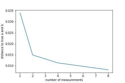
(a) Forward KL conditional DeepGEM.

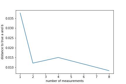
(b) Reverse KL conditional DeepGEM.

Figure 1: Distance to the hyperparameters (a,b) for forward and reverse KL conditional DeepGEM.

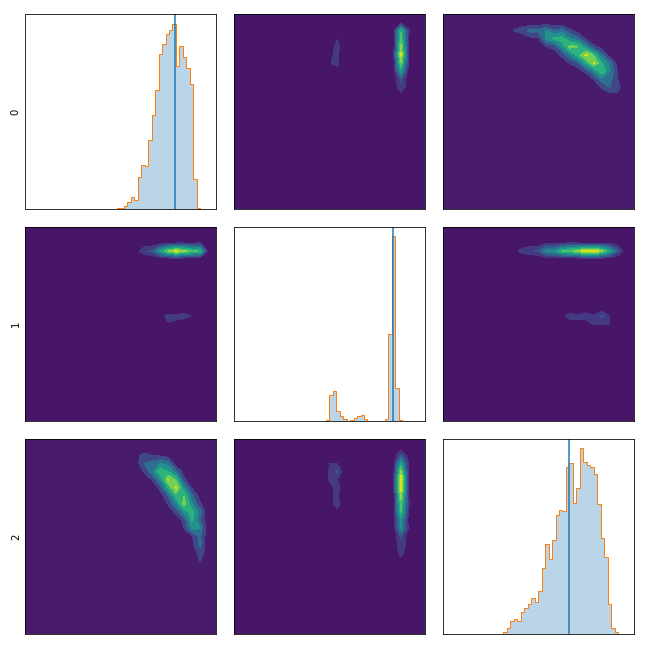
(a) Posterior reconstruction for forward KL conditional DeepGEM for measurement 1.

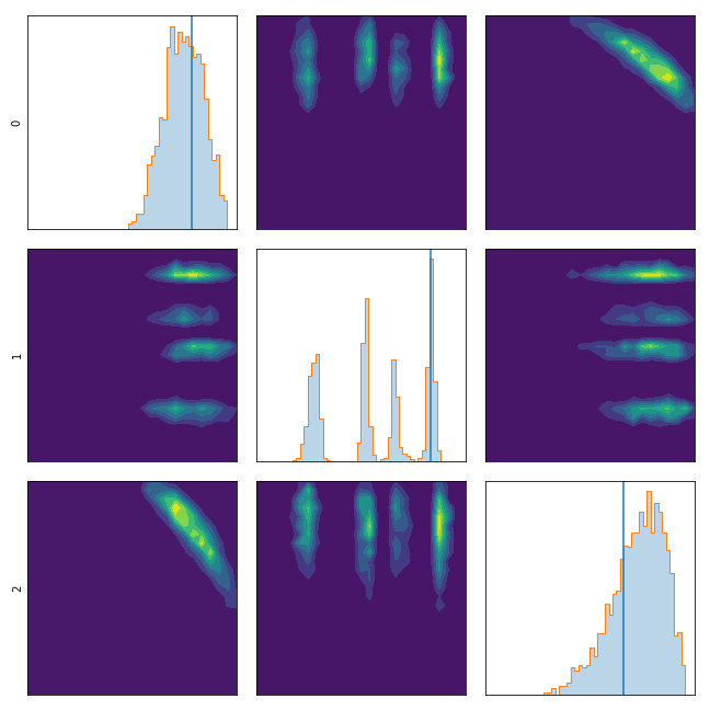
(b) Posterior reconstruction for reverse KL conditional DeepGEM for measurement 1.

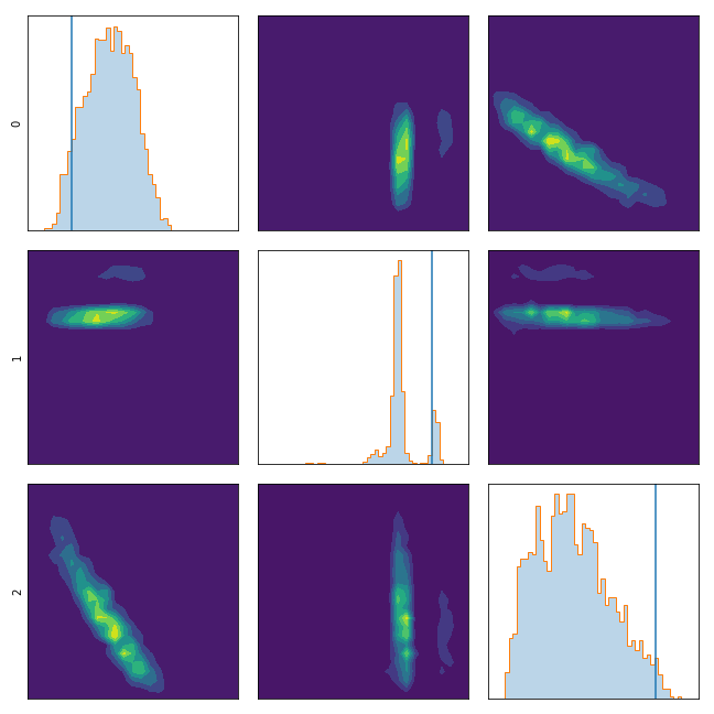
(c) Posterior reconstruction for forward KL conditional DeepGEM for measurement 2.

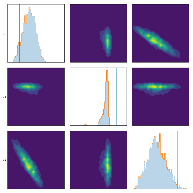
(d) Posterior reconstruction for reverse KL conditional DeepGEM for measurement 2.

Figure 2: Posterior reconstructions for different measurements using forward/reverse conditional DeepGEM. Ground truth x is depicted by the blue line.

Line grating with oxid layer

The second example involves a line grating consisting of a silicon bulk and an oxide layer on top, investigated e.g. in [39]. In addition to the geometry parameters, as used in the previous example, the optical constants (OC) of the materials are assumed to be not accurately known. In practice this is often the case if the material composition was changed due to oxidation and contamination of the sample. Therefore for each material, there are two parameters for the complex refractive index (real and imaginary part), which depend on the material density. Hence we change the OC by varying the densities of the material, i.e. silicon and silicon-oxide. This results in two parameters changing the OC and five parameter describing the geometry of the line grating. The refraction pattern are detected for a single energy of the incoming light beam under a angle of incidence of 30° and a set of seven azimuth angles between 0° and 6 °. In sum we obtained 77 simulated intensities and hence end up with x-dimension seven and y-dimension 77. For the simulation a forward model was defined with the software package JCMsuite, based on a FEM which solves a boundary value problem following from the Maxwell’s equations [20]. In order to get a strong response for the OC of the oxide layer we used an energy of 95.4eV, right before the absorption edge [3]. For this work we standardized the data from the forward simulation [10] on $[0,1]$ and chose an uniform prior for the $x$-data. Again, we plot two exemplary posterior distribution calculated. The distribution shapes seen in 4 clearly reflect the sensitivity of the forward operator against the line height (parameter 0), the silicon oxide density (parameter 4) and non-sensitive against the layer roughness (parameter 6). The true $a$ and $b$ were set to $0.03$ and $0.25$ respectively. Again as in the first scatterometry example we can see in Table 3 and 4 that the forward KL performs better in distance to the true a and b as well as ELBO. Similarly, one can see that the first x-component, the height can be multimodal, where the reverse KL can indeed miss the mode. This can be observed in Fig. 4. Similarly, the distance to the true a and b decreases by adding more simulated measurement values, which can be seen in Fig. 3.

number measurements	1	2	4	8
forward	0.24	0.052	0.021	0.019
reverse	0.24	0.08	0.04	0.028

Table 3: Distance of estimated $a$ and $b$ to the true ones over 5 runs.

number measurements	1	2	4	8
forward	193.8	191.9	168.8	184.4
reverse	189.7	189.3	168.5	183.8

Table 4: ELBO of the algorithms over 5 runs. Calculated for the measurements based on 2000 samples.

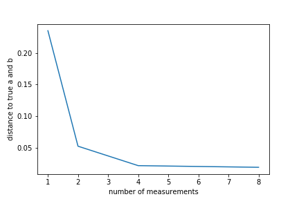
(a) Forward KL conditional DeepGEM.

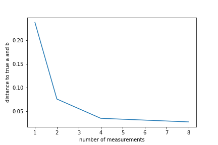
(b) Reverse KL conditional DeepGEM.

Figure 3: Distance to the hyperparameters (a,b) for forward and reverse KL conditional DeepGEM.

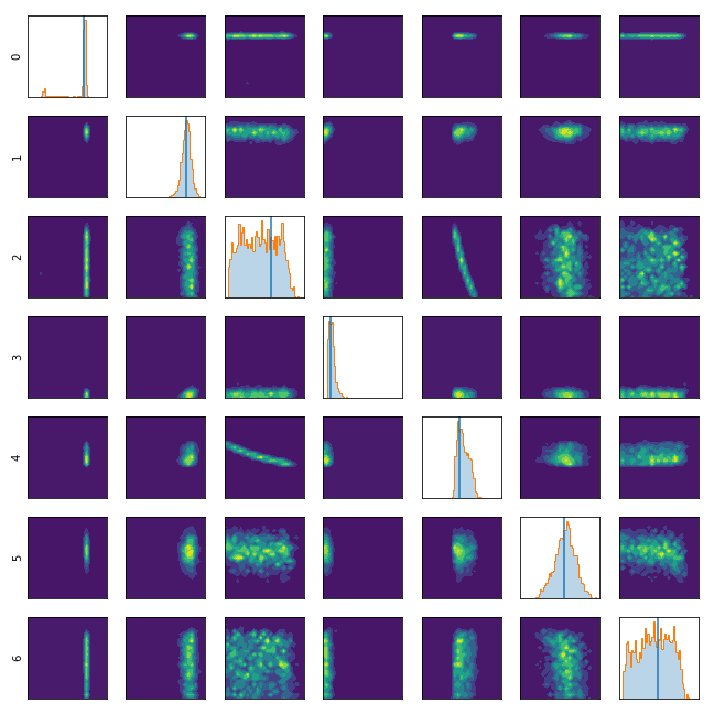
(a) Posterior reconstruction for forward KL conditional DeepGEM for measurement 1.

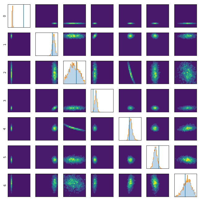
(b) Posterior reconstruction for reverse KL conditional DeepGEM for measurement 1.

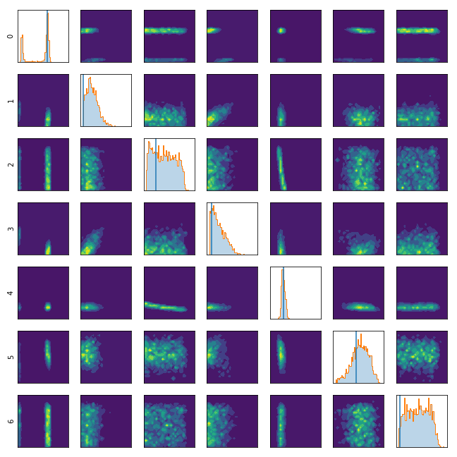
(c) Posterior reconstruction for forward KL conditional DeepGEM for measurement 2.

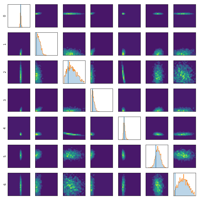
(d) Posterior reconstruction for reverse KL conditional DeepGEM for measurement 2.

Figure 4: Posterior reconstructions for different measurements using forward/reverse conditional DeepGEM.

5 Conclusions and Limitations

We developed a nested EM algorithms, one for estimating the posterior distribution via a conditional NF and a second one to solve the M-step within the former EM algorithm to estimate the error model parameters. For the special kind of non-additive noise appearing in our applications we derived analytic formulas for the inner E- and M-steps. We showed advantages of using the forward KL for modelling multimodal distributions. The reverse KL often led to mode collapse. However, there has been a plethora of literature tackling this issue of the reverse KL, namely [4, 42, 57, 40]. It would be interesting to compare these approaches to the forward KL. Moreover, we could replace the conditional normalizing flow by other methods for posterior sampling like score-based diffusion models [31, 53], conditional GANs [44] or posterior MMD flows [22]. Furthermore, we chose synthetic $a_{true}$ and $b_{true}$. One of the next steps is to test these approaches on real world measurements. Even if the novel algorithm was applied to two specific real world experiments, it may have an impact to a wide range of applications where indirect measurements are involved. The extension of the algorithm to other noise distributions than Gaussian is analogous. An advantage over standard approaches like Markov-Chain Monte Carlo methods is the fact that once the network has been trained, further similar measurements can be evaluated very quickly. This benefit opens the possibility of scatterentry and similar measurement techniques for real time applications, e.g. important for process control. In terms of limitations, it would be also interesting to test the algorithm on other inverse problems. Intuitively, we believe that the scatterometric inverse problem is particularly well-suited for these estimations since the observed $f(X)$-data is living on a low-dimensional manifold in a nominal high-dimensional space. One can indeed easily think of an inverse problem, where recovering noise parameters is much harder if the observed data already lies in the full space.

Acknowledgements

P.H. acknowledges support from the DFG within the SPP 2298 "Theoretical Foundations of Deep Learning" (STE 571/17-1). J.H. acknowledges funding by the EPSRC programme grant “The Mathematics of Deep Learning” with reference EP/V026259/1. M.C. and S.H. acknowledges the support of the EMPIR project 22IND04-ATMOC. This project (20IND04 ATMOC) has received funding from the EMPIR programme cofinanced by the Participating States and from the European Union’s Horizon 2020 research and innovation programme.

Appendix A Derivation of the inner M-step

For the simplicity of the notation, we use the abbreviation

$$Q_{i}=P_{V_{\theta^{(r)}}|(X,Y_{\theta^{(r)}})=(x_{i},y_{i})}=\mathcal{N}\Big{(}\tfrac{(a^{(r)})^{2}(y_{i}-F(x_{i}))}{(a^{(r)})^{2}+(b^{(r)})^{2}F(x_{i})^{2}},\mathrm{diag}\big{(}\tfrac{(a^{(r)})^{2}(b^{(r)})^{2}F(x_{i})^{2}}{(a^{(r)})^{2}+(b^{(r)})^{2}F(x_{i})^{2}}\big{)}\Big{)}.$$ (23)

Using the decomposition (8) of the ELBO, and noting that the second summand within (8) does not depend on the parameters $\theta=(a,b)$, we obtain that the optimization problem (6) is equivalent to

$$\theta^{(r+1)} =\operatorname*{arg\,max}_{\theta\in\Theta}\sum_{i=1}^{N}\frac{1}{N}\mathbb{E}_{v\sim Q_{i}}[\log(p_{V_{\theta},X,Y_{\theta}}(v,x_{i},y_{i}))]$$ (24)

$$=\operatorname*{arg\,max}_{\theta\in\Theta}\sum_{i=1}^{N}\frac{1}{N}\mathbb{E}_{v\sim Q_{i}}[\log(p_{V_{\theta},Y_{\theta}|X=x_{i}}(v,y_{i}))]+\log(p_{X}(x_{i}))$$

$$=\operatorname*{arg\,max}_{\theta\in\Theta}\sum_{i=1}^{N}\frac{1}{N}\mathbb{E}_{v\sim Q_{i}}[\log(p_{V_{\theta},Y_{\theta}|X=x_{i}}(v,y_{i}))]$$

Now, the objective function reads as

$$\quad\sum_{i=1}^{N}\frac{1}{N}\mathbb{E}_{v\sim Q_{i}}[\log(p_{V_{\theta},Y_{\theta}|X=x_{i}}(v,y_{i}))]$$ (25)

$$=\sum_{i=1}^{N}\frac{1}{N}\mathbb{E}_{v\sim Q_{i}}[\log(p_{Y_{\theta}|V_{\theta}=v,X=x_{i}}(y_{i}))+\log(p_{V_{\theta}|X=x_{i}}(v))].$$ (26)

As it holds by definition that $p_{Y_{\theta}|V_{\theta}=v,X=x_{i}}(y_{i})=\mathcal{N}(y_{i}|F(x_{i})+v,b^{2}\mathrm{diag}(F(x))^{2})$ and $p_{V_{\theta}|X=x_{i}}(v)=p_{V_{\theta}}(v)=\mathcal{N}(v|0,a^{2}I_{n})$, this is equal to

$$\quad\sum_{i=1}^{N}\frac{1}{N}\mathbb{E}_{v\sim Q_{i}}[\log(\mathcal{N}(y_{i}|F(x_{i})+v,b^{2}\mathrm{diag}(F(x))^{2})+\log(\mathcal{N}(v|0,a^{2}I))]=A_{1}(b)+A_{2}(a),$$ (27)

where

$$A_{1}(b) =\sum_{i=1}^{N}\mathbb{E}_{v\sim Q_{i}}[\log(\mathcal{N}(y_{i}|f(x_{i})+v,b^{2}\mathrm{diag}(F(x))^{2})]$$

$$=-\frac{1}{2b^{2}}\sum_{i=1}^{N}\sum_{j=1}^{n}\frac{\frac{1}{N}}{F_{j}(x_{i})^{2}}\Big{(}(y_{ij}-F_{j}(x))^{2}-2\mathbb{E}_{v\sim Q_{i}}[v_{j}](y_{ij}-F_{j}(x))+\mathbb{E}_{v\sim Q_{i}}[v_{j}^{2}]\Big{)}$$

$$\quad-\sum_{i=1}^{N}\sum_{j=1}^{n}\frac{1}{N}\log(|F_{j}(x)|)-\frac{nN}{2}\log(2\pi b^{2}),$$

and

$$A_{2}(a) =\sum_{i=1}^{N}\frac{1}{N}\mathbb{E}_{v\sim Q_{i}}[\log(\mathcal{N}(v|0,a^{2}I))]=-\frac{1}{2a^{2}}\sum_{i=1}^{N}\sum_{j=1}^{n}\mathbb{E}_{v\sim Q_{i}}[v_{j}^{2}]-\frac{nN}{2}\log(2\pi a^{2}).$$ (28)

Now, by (23), the expressions $\mathbb{E}_{v\sim Q_{i}}[v_{j}]$ and $\mathbb{E}_{v\sim Q_{i}}[v_{j}^{2}]$ are the first and second moment of certain normal distributions, such that

$$\mathbb{E}_{v\sim Q_{i}}[v_{j}]=\frac{(a^{(r)})^{2}(y_{ij}-F_{j}(x_{i}))}{(a^{(r)})^{2}+(b^{(r)})^{2}F_{j}(x_{i})^{2}}$$

and

$$\mathbb{E}_{v\sim Q_{i}}[v_{j}^{2}]=\Big{(}\frac{(a^{(r)})^{2}(y_{ij}-F_{j}(x_{i}))}{(a^{(r)})^{2}+(b^{(r)})^{2}F_{j}(x_{i})^{2}}\Big{)}^{2}+\frac{(a^{(r)})^{2}(b^{(r)})^{2}F_{j}(x_{i})^{2}}{(a^{(r)})^{2}+(b^{(r)})^{2}F_{j}(x_{i})^{2}}.$$

Putting everything together, we obtain that (24) is equivalent to

$$\theta^{(r+1)}=\operatorname*{arg\,max}_{(a,b)\in\mathbb{R}^{2}_{\geq 0}}A_{1}(b)+A_{2}(a)$$

with

$$A_{1}(b)=\frac{1}{2b^{2}}c_{1}^{(r)}-nN\log(b)+\mathrm{const},\quad A_{2}(a)=\frac{1}{2a^{2}}c_{2}^{(r)}-nN\log(a)+\mathrm{const},$$

where $\mathrm{const}$ denotes an unspecified constant independent of $a$ and $b$. Further, the $c_{i}^{(r)}$ are given by

$$c_{2}^{(r)}=-\sum_{i=1}^{N}\frac{1}{N}\bigg{(}\sum_{j=1}^{n}\Big{(}\frac{(a^{(r)})^{2}(y_{ij}-F_{j}(x_{i}))}{(a^{(r)})^{2}+(b^{(r)})^{2}F_{j}(x_{i})^{2}}\Big{)}^{2}+\frac{(a^{(r)}b^{(r)}F_{j}(x_{i}))^{2}}{(a^{(r)})^{2}+(b^{(r)}F_{j}(x_{i}))^{2}}\bigg{)},$$ (29)

and

$$c_{1}^{(r)} =-\sum_{i=1}^{N}\sum_{j=1}^{n}\frac{\frac{1}{N}}{F_{j}(x_{i})^{2}}\Big{(}(y_{ij}-F_{j}(x_{i}))^{2}-2\frac{(a^{(r)})^{2}(y_{ij}-F_{j}(x_{i}))^{2}}{(a^{(r)})^{2}+(b^{(r)})^{2}F_{j}(x_{i})^{2}}$$ (30)

$$\quad+\Big{(}\frac{(a^{(r)})^{2}(y_{ij}-F_{j}(x_{i}))}{(a^{(r)})^{2}+(b^{(r)})^{2}F_{j}(x_{i})^{2}}\Big{)}^{2}+\frac{(a^{(r)}b^{(r)}F_{j}(x_{i}))^{2}}{(a^{(r)})^{2}+(b^{(r)}F_{j}(x_{i}))^{2}}\Big{)}.$$ (31)

Bringing the first three terms onto one denominator, this can be simplified to

$$c_{1}^{(r)} =-\sum_{i=1}^{N}\sum_{j=1}^{n}\frac{\frac{1}{N}(y_{ij}-F_{j}(x_{i}))^{2}(b^{(r)})^{4}F_{j}(x_{i})^{2}}{((a^{(r)})^{2}+(b^{(r)}F_{j}(x_{i}))^{2})^{2}}+\frac{\frac{1}{N}(a^{(r)}b^{(r)})^{2}}{(a^{(r)})^{2}+(b^{(r)}F_{j}(x_{i}))^{2}}.$$ (32)

Note that by definition $c_{i}^{(r)}$, $i=1,2$ are non-positive. Thus, $a^{(r+1)}$ and $b^{(r+1)}$ are given by

$$a^{(r+1)}=\operatorname*{arg\,max}_{a\geq 0}A_{2}(a),\qquad b^{(r+1)}=\operatorname*{arg\,max}_{b\geq 0}A_{1}(b).$$

By setting the derivatives of $A_{1}$ and $A_{2}$ to zero, this is equivalent to

$$a^{(r+1)}=-\frac{c_{2}^{(r)}}{nN},\qquad b^{(r+1)}=-\frac{c_{1}^{(r)}}{nN}.$$

Appendix B Sensitivity analysis of the forward model

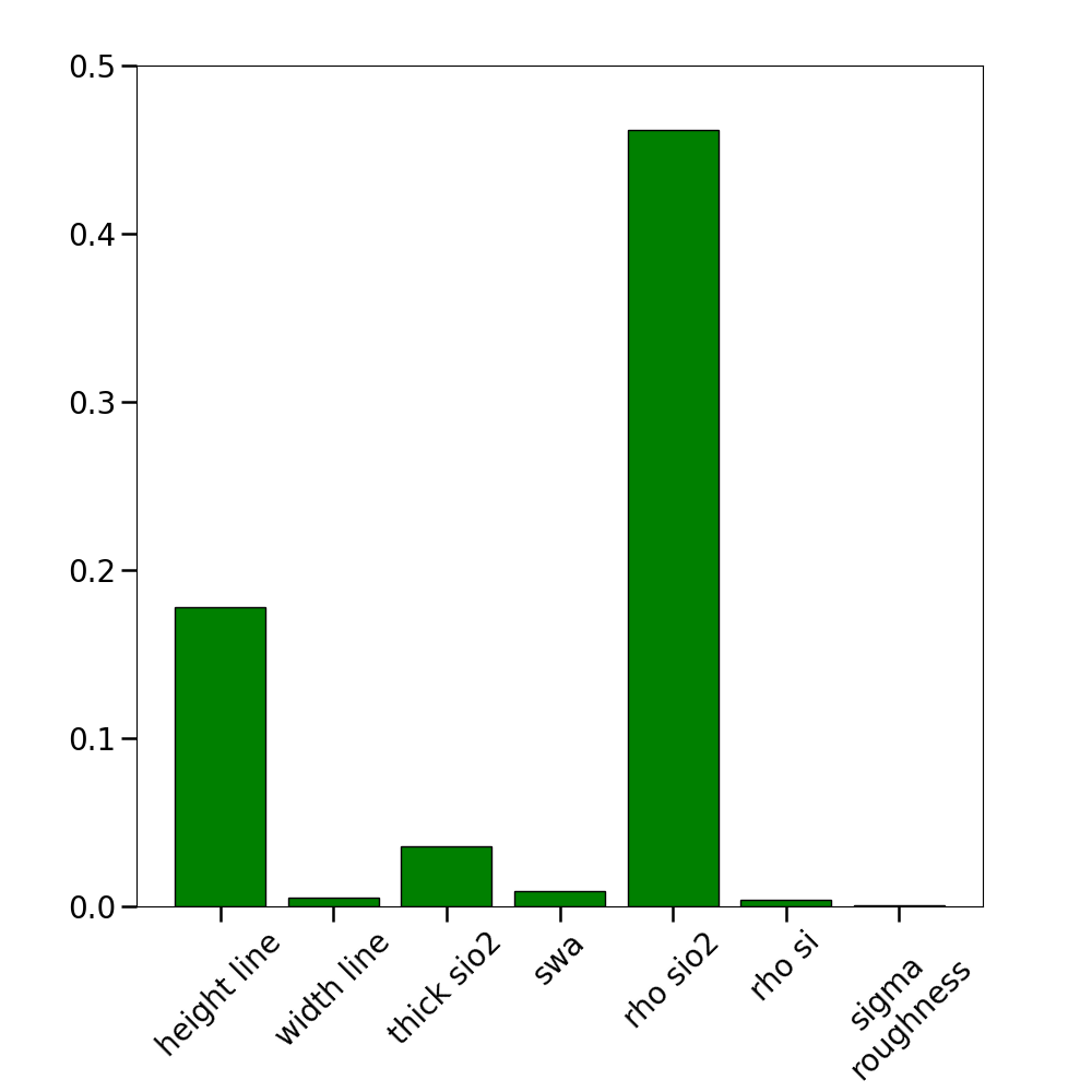
Figure 5: Barplot of sobol‘ indices for PC-expansion of the forward model.

To verify our results for the reconstruction of the line grating in 4, we make a sensitivity analysis (SA) of the corresponding forward model. For the SA we have to determine the Sobol‘ indices, which are coefficients of a decomposition of the forward model and describe the impact of each parameter combination on the forward model. Those indices are normalized to $[0,1]$ and sum up to $1$ [55], [54]. Making an approximation of the forward model in a polynomial basis using Polynomial Chaos (PC) [58],[20] makes it very easy to calculate the Sobol‘ indices. The indices in Fig. 5 come from a PC-approximation with a relative $L_{2}$-error of about $0.076$ and show the dependence on each single parameter. It is clearly seen, that the height of the grating line and the density of the oxide layer and hence the OC for silicon-oxide has a huge impact on the forward model. In general the SA fits very well to the reconstruction of the line grating, since in Fig. 5 the distributions for parameter $0$ and $4$ are very sharp defined, while those which are very broad distributed also show a low impact on the forward model. For the SA the source software tool PyThia was used [25].

References

- [1] F. Altekrüger and J. Hertrich. WPPNets and WPPFlows: The power of Wasserstein patch priors for superresolution. SIAM Journal on Imaging Sciences, 16(3):1033–1067, 2023.
- [2] A. Andrle, N. Farchmin, P. Hagemann, S. Heidenreich, V. Soltwisch, and G. Steidl. Invertible neural networks versus mcmc for posterior reconstruction in grazing incidence x-ray fluorescence. In International Conference on Scale Space and Variational Methods in Computer Vision, pages 528–539. Springer, 2021.
- [3] A. Andrle, P. Hönicke, J. Vinson, R. Quintanilha, Q. Saadeh, S. Heidenreich, F. Scholze, and V. Soltwisch. The anisotropy in the optical constants of quartz crystals for soft X-rays. J Appl Crystallogr, 54(2):402–408, Apr. 2021.
- [4] M. Arbel, A. G. D. G. Matthews, and A. Doucet. Annealed flow transport monte carlo. In Proceedings of the 38th International Conference on Machine Learning, Proceedings of Machine Learning Research, 18–24 Jul 2021.
- [5] L. Ardizzone, T. Bungert, F. Draxler, U. Köthe, J. Kruse, R. Schmier, and P. Sorrenson. Framework for Easily Invertible Architectures (FrEIA), 2018-2022.
- [6] L. Ardizzone, C. Lüth, J. Kruse, C. Rother, and U. Köthe. Guided image generation with conditional invertible neural networks. ArXiv:1907.02392, 2019.
- [7] J. Behrmann, W. Grathwohl, R. T. Chen, D. Duvenaud, and J.-H. Jacobsen. Invertible residual networks. In International Conference on Machine Learning, pages 573–582, 2019.
- [8] C. M. Bishop. Pattern Recognition and Machine Learning (Information Science and Statistics). Springer-Verlag, Berlin, Heidelberg, 2006.
- [9] C. M. Bishop and N. M. Nasrabadi. Pattern Recognition and Machine Learning. Springer, 2006.
- [10] M. Casfor. Forward simulation of scatterometry for a nanostructure. https://zenodo.org/doi/10.5281/zenodo.10580011, Feb. 2024. [Data set].
- [11] R. T. Q. Chen, J. Behrmann, D. K. Duvenaud, and J.-H. Jacobsen. Residual flows for invertible generative modeling. In Advances in Neural Information Processing Systems, volume 32. Curran Associates, Inc., 2019.
- [12] S. Chrétien and A. O. Hero. Kullback proximal algorithms for maximum-likelihood estimation. IEEE Transactions on Information Theory, 46(5):1800–1810, 2000.
- [13] S. Chrétien and A. O. Hero. On EM algorithms and their proximal generalizations. ESAIM: Probability and Statistics, 12:308–326, 2008.
- [14] N. De Cao, I. Titov, and W. Aziz. Block neural autoregressive flow. ArXiv:1904.04676, 2019.
- [15] A. P. Dempster, N. M. Laird, and D. B. Rubin. Maximum likelihood from incomplete data via the EM algorithm. Journal of the Royal Statistical Society. Series B (Methodological), 39(1):1–38, 1977.
- [16] A. Denker, M. Schmidt, J. Leuschner, and P. Maass. Conditional invertible neural networks for medical imaging. Journal of Imaging, 7(11):243, 2021.
- [17] L. Dinh, J. Sohl-Dickstein, and S. Bengio. Density estimation using real NVP. In International Conference on Learning Representations, 2017.
- [18] M. M. Dunlop. Multiplicative noise in bayesian inverse problems: Well-posedness and consistency of map estimators. arxiv preprint arXiv: 1910.14632, 2019.
- [19] C. Durkan, A. Bekasov, I. Murray, and G. Papamakarios. Neural spline flows. Advances in Neural Information Processing Systems, 2019.
- [20] N. Farchmin, M. Hammerschmidt, P.-I. Schneider, M. Wurm, B. Bodermann, M. Bär, and S. Heidenreich. An efficient approach to global sensitivity analysis and parameter estimation for line gratings. Modeling Aspects in Optical Metrology VII, page 15, June 2019.
- [21] A. F. Gao, J. C. Castillo, Y. Yue, Z. E. Ross, and K. L. Bouman. DeepGEM: Generalized expectation-maximization for blind inversion. In Advances in Neural Information Processing Systems, volume 35, 2021.
- [22] P. Hagemann, J. Hertrich, F. Altekrüger, R. Beinert, J. Chemseddine, and G. Steidl. Posterior sampling based on gradient flows of the MMD with negative distance kernel. ICLR 2024 and arXiv preprint arXiv:2310.03054, 2024.
- [23] P. Hagemann, J. Hertrich, and G. Steidl. Stochastic normalizing flows for inverse problems: a Markov chains viewpoint. SIAM/ASA Journal on Uncertainty Quantification, 10(3):1162–1190, 2022.
- [24] P. Hagemann, J. Hertrich, and G. Steidl. Generalized Normalizing Flows via Markov Chains. Cambridge University Press, 2023.
- [25] N. Hegemann and S. Heidenreich. Pythia: A python package for uncertainty quantification based on non-intrusive polynomial chaos expansions. Journal of Open Source Software, 8(89):5489, 2023.
- [26] S. Heidenreich, H. Gross, and M. Bär. Bayesian approach to the statistical inverse problem of scatterometry: Comparison of three surrogate models. Int. J. Uncertain. Quantif., 5(6), 2015.
- [27] S. Heidenreich, H. Gross, and M. Bär. Bayesian approach to determine critical dimensions from scatterometric measurements. Metrologia, 55(6):S201, Dec. 2018.
- [28] A. F. Herrero, M. Pflüger, J. Puls, F. Scholze, and V. Soltwisch. Uncertainties in the reconstruction of nanostructures in euv scatterometry and grazing incidence small-angle x-ray scattering. Optics Express, 29(22):35580–35591, 2021.
- [29] J. Hertrich. Proximal residual flows for Bayesian inverse problems. In International Conference on Scale Space and Variational Methods in Computer Vision, pages 210–222. Springer, 2023.
- [30] F. Hirschberger, D. Forster, and J. Lucke. A variational em acceleration for efficient clustering at very large scales. IEEE Transactions on Pattern Analysis and Machine Intelligence, 2021.
- [31] J. Ho, A. Jain, and P. Abbeel. Denoising diffusion probabilistic models. Advances in neural information processing systems, 33:6840–6851, 2020.
- [32] C.-W. Huang, D. Krueger, A. Lacoste, and A. Courville. Neural autoregressive flows. In International Conference on Machine Learning, pages 2078–2087, 2018.
- [33] H.-T. Huang and F. L. Terry Jr. Spectroscopic ellipsometry and reflectometry from gratings (scatterometry) for critical dimension measurement and in situ, real-time process monitoring. Thin Solid Films, 455:828–836, 2004.
- [34] D. P. Kingma and J. Ba. Adam: A method for stochastic optimization. arXiv preprint arXiv:1412.6980, 2017.
- [35] D. P. Kingma and P. Dhariwal. Glow: Generative flow with invertible 1x1 convolutions. ArXiv:1807.03039, 2018.
- [36] J. Kruse, G. Detommaso, R. Scheichl, and U. Köthe. HINT: Hierarchical invertible neural transport for density estimation and Bayesian inference. ArXiv:1905.10687, 2020.
- [37] C. Laroche, A. Almansa, and E. Coupeté. Fast diffusion em: A diffusion model for blind inverse problems with application to deconvolution. In Proceedings of the IEEE/CVF Winter Conference on Applications of Computer Vision (WACV), pages 5271–5281, January 2024.
- [38] C. Liu and D. B. Rubin. The ecme algorithm: a simple extension of em and ecm with faster monotone convergence. Biometrika, 81(4):633–648, 1994.
- [39] L. M. Lohr, R. Ciesielski, S. Glabisch, S. Schröder, S. Brose, and V. Soltwisch. Nanoscale grating characterization using euv scatterometry and soft x-ray scattering with plasma and synchrotron radiation. Applied Optics, 62(1):117–132, 2023.
- [40] B. Máté and F. Fleuret. Learning interpolations between boltzmann densities. Transactions on Machine Learning Research, 2023.
- [41] X.-L. Meng and D. B. Rubin. Maximum likelihood estimation via the ecm algorithm: A general framework. Biometrika, 80(2):267–278, 1993.
- [42] L. I. Midgley, V. Stimper, G. N. C. Simm, B. Schölkopf, and J. M. Hernández-Lobato. Flow annealed importance sampling bootstrap. In The Eleventh International Conference on Learning Representations, 2023.
- [43] T. Minka. Technical report, Microsoft Research, 2005.
- [44] M. Mirza and S. Osindero. Conditional generative adversarial nets. arXiv preprint arXiv:1411.1784, 2014.
- [45] A. Mohammad-Djafari. On the estimation of hyperparameters in bayesian approach of solving inverse problems. In 1993 IEEE International Conference on Acoustics, Speech, and Signal Processing, volume 5, pages 495–498 vol.5, 1993.
- [46] Y. Nan, Y. Quan, and H. Ji. Variational-EM-based deep learning for noise-blind image deblurring. In Proceedings of the IEEE/CVF Conference on Computer Vision and Pattern Recognition (CVPR), June 2020.
- [47] R. M. Neal and G. E. Hinton. A view of the em algorithm that justifies incremental, sparse, and other variants. In Learning in graphical models, pages 355–368. Springer, 1998.
- [48] G. Papamakarios, T. Pavlakou, , and I. Murray. Masked autoregressive flow for density estimation. Advances in Neural Information Processing Systems, page 2338–2347, 2017.
- [49] A. Paszke, S. Gross, F. Massa, A. Lerer, J. Bradbury, G. Chanan, T. Killeen, Z. Lin, N. Gimelshein, L. Antiga, A. Desmaison, A. Kopf, E. Yang, Z. DeVito, M. Raison, A. Tejani, S. Chilamkurthy, B. Steiner, L. Fang, J. Bai, and S. Chintala. Pytorch: An imperative style, high-performance deep learning library. In H. Wallach, H. Larochelle, A. Beygelzimer, F. d'Alché-Buc, E. Fox, and R. Garnett, editors, Advances in Neural Information Processing Systems, volume 32. Curran Associates, Inc., 2019.
- [50] D. M. Rocke and B. Durbin. A model for measurement error for gene expression arrays. Journal of computational biology, 8(6):557–569, 2001.
- [51] D. M. Rocke and S. Lorenzato. A two-component model for measurement error in analytical chemistry. Technometrics, 37(2):176–184, 1995.
- [52] Q. Saadeh, P. Naujok, V. Philipsen, P. Hönicke, C. Laubis, C. Buchholz, A. Andrle, C. Stadelhoff, H. Mentzel, A. Schönstedt, et al. Time-frequency analysis assisted determination of ruthenium optical constants in the sub-euv spectral range 8 nm–23.75 nm. Optics Express, 29(25):40993–41013, 2021.
- [53] I. R. Singh, A. Denker, R. Barbano, Ž. Kereta, B. Jin, K. Thielemans, P. Maass, and S. Arridge. Score-based generative models for PET image reconstruction. arXiv preprint arXiv:2308.14190, 2023.
- [54] I. Sobol. Sensitivity Estimates for Nonlinear Mathematical Models. MMCE, 1:407–414, 1993.
- [55] I. Sobol. Global sensitivity indices for nonlinear mathematical models and their Monte Carlo estimates. Mathematics and Computers in Simulation, 55(1-3):271–280, Feb. 2001.
- [56] H. Sun and K. L. Bouman. Deep probabilistic imaging: Uncertainty quantification and multi-modal solution characterization for computational imaging. In Proceedings of the AAAI Conference on Artificial Intelligence, volume 35, pages 2628–2637, 2021.
- [57] L. Vaitl, K. A. Nicoli, S. Nakajima, and P. Kessel. Gradients should stay on path: better estimators of the reverse- and forward kl divergence for normalizing flows. Machine Learning: Science and Technology, 3(4):045006, oct 2022.
- [58] N. Wiener. The Homogeneous Chaos. American Journal of Mathematics, 60(4):897, Oct. 1938.
- [59] C. Winkler, D. Worrall, E. Hoogeboom, and M. Welling. Learning likelihoods with conditional normalizing flows. arXiv preprint arXiv:1912.00042, 2023.
- [60] H. Wu, J. Köhler, and F. Noé. Stochastic normalizing flows. Advances in Neural Information Processing Systems, 33:5933–5944, 2020.