Dynamic Byzantine-Robust Learning: Adapting to Switching Byzantine Workers

Abstract

Byzantine-robust learning has emerged as a prominent fault-tolerant distributed machine learning framework. However, most techniques consider the static setting, wherein the identity of Byzantine machines remains fixed during the learning process. This assumption does not capture real-world dynamic Byzantine behaviors, which may include transient malfunctions or targeted temporal attacks. Addressing this limitation, we propose DynaBRO – a new method capable of withstanding $\mathcal{O}(\sqrt{T})$ rounds of Byzantine identity alterations (where $T$ is the total number of training rounds), while matching the asymptotic convergence rate of the static setting. Our method combines a multi-level Monte Carlo (MLMC) gradient estimation technique with robust aggregation of worker updates and incorporates a fail-safe filter to limit bias from dynamic Byzantine strategies. Additionally, by leveraging an adaptive learning rate, our approach eliminates the need for knowing the percentage of Byzantine workers.

1 Introduction

Recently, there has been an increasing interest in large-scale distributed machine learning (ML), where multiple machines (i.e., workers) collaboratively aim at minimizing some global objective under the coordination of a central server (Verbraeken et al., 2020; Kairouz et al., 2021). This approach, leveraging the collective power of multiple computation nodes, holds the promise of significantly reducing training times for complex ML models, such as large language models (Brown et al., 2020). However, the growing reliance on distributed ML systems exposes them to potential errors, faults, malfunctions, and even adversarial attacks. These Byzantine faults pose a significant risk to the integrity of the learning process and could lead to reduced reliability and accuracy in the predictions of the resulting models (Lamport et al., 2019; Guerraoui et al., 2023).

Due to its significance in distributed ML, Byzantine fault-tolerance has attracted considerable interest. Indeed, many prior works have focused on Byzantine-robust learning, aiming to ensure effective learning in the presence of Byzantine machines. These efforts have led to the development of algorithms capable of enduring Byzantine attacks (Feng et al., 2014; Su and Vaidya, 2016; Blanchard et al., 2017; Chen et al., 2017; Alistarh et al., 2018; Guerraoui et al., 2018; Yin et al., 2018; Allen-Zhu et al., 2020; Karimireddy et al., 2021; 2022; Farhadkhani et al., 2022; Allouah et al., 2023).

While the existing body of research has significantly advanced the understanding of Byzantine-robust learning, a notable gap persists in the treatment of the setting. The vast majority of research in this area has focused on the static setting, wherein the identity of Byzantine machines remains fixed throughout the entire learning process. Nevertheless, real-world distributed learning systems may often encounter dynamic Byzantine behaviors, where machines exhibit erratic and unpredictable fault patterns. Despite the importance of these scenarios, the investigation of robustness against such dynamic behaviors remains underexplored.

In federated learning, for instance, the concept of partial participation inherently introduces a dynamic aspect (Bonawitz et al., 2019; Kairouz et al., 2021). Workers join and leave the training process, leading to a scenario where a Byzantine worker might be present in one round and absent in the next. In fact, the same node might switch between honest and Byzantine behaviors; such fluctuations could stem from strategic manipulations by an adversary seeking to evade detection, or due to software updates that inadvertently trigger or resolve certain security vulnerabilities.

Such vulnerabilities may also be relevant in distributed training within multi-tenant data centers or across volunteer computing paradigms (Kijsipongse et al., 2018; Ryabinin and Gusev, 2020; Atre et al., 2021). In multi-tenant data centers, the sharing of resources among users inherently increases exposure to security vulnerabilities and version inconsistencies. Similarly, volunteer computing paradigms, characterized by a large pool of less reliable workers and regular occurrences of node failures, are susceptible to dynamic fault patterns. The prolonged training times of complex ML models in these settings often result in intermittent node failures, typically due to hardware issues, network instabilities, or maintenance activities. These representative examples of dynamic Byzantine behaviors pose challenges that the conventional static approach fails to address.

Previous research has established that convergence is unattainable when Byzantine workers can change their identities in each round (Karimireddy et al., 2021). However, it remains unclear how a limited number of identity-switching rounds affects the convergence rate. This work addresses this challenge by introducing a new method, DynaBRO. We establish its convergence, highlighting that the rates degrade linearly with the number of rounds featuring Byzantine behavior alterations. Specifically, this implies that our method can endure $\mathcal{O}(\sqrt{T})$ such rounds, where $T$ is the total number of training rounds, while matching the asymptotic convergence rate of the static setting. Moreover, by employing an adaptive learning rate, we can further eliminate the need for prior knowledge of the objective smoothness and fraction of Byzantine workers, thus increasing practicality.

The key ingredient of our approach is a multi-level Monte Carlo (MLMC) gradient estimation technique (Dorfman and Levy, 2022; Beznosikov et al., 2023), serving as a bias-reduction tool. In Section 3, we show that combining it with a general $(\delta,\kappa)$-robust aggregator (Allouah et al., 2023) mitigates the bias introduced by Byzantine workers in the static setting, an analysis of independent interest. Transitioning to the dynamic setting in Section 4, we refine the MLMC estimator with an added fail-safe filter to prevent a malicious adversary from exploiting its structure and injecting large bias. This modification is crucial given the estimator’s reliance on multiple consecutive samples, which renders it susceptible to dynamic Byzantine changes. Finally, in Section 5, we turn our focus to optimality and adaptivity. The introduction of a new aggregation rule allows us to derive asymptotically optimal convergence bounds (for a restricted number of identity-switching rounds). In addition, employing an adaptive learning rate enables us to eliminate the need for prior knowledge of the objective smoothness and the fraction of Byzantine workers.

2 Preliminaries and Related Work

In this section, we formalize our objective, specify our assumptions, and overview relevant related work.

2.1 Problem Formulation and Assumptions

We consider stochastic optimization, where our objective is to minimize the expected loss given some unknown data distribution $\mathcal{D}$ and a set of loss functions $\left\{x\mapsto F(\cdot;\xi)\right\}$ parameterized by $\xi\sim\mathcal{D}$. Formally, our goal is to solve:

$$\min_{x\in\mathcal{K}}{f(x)\coloneqq\mathbb{E}_{\xi\sim\mathcal{D}}\left[F(x;\xi)\right]}\;,$$ (1)

where $\mathcal{K}\subseteq{\mathbb{R}}^{d}$ is the optimization domain. To this end, we assume there are $m$ workers (i.e., machines), each with access to samples from $\mathcal{D}$. This homogeneous setting was previously studied in the context of Byzantine-robust learning (Blanchard et al., 2017; Alistarh et al., 2018; Allen-Zhu et al., 2020), and it is realistic in collaborative learning, where workers may have access to the entire data (Kijsipongse et al., 2018; Diskin et al., 2021; Gorbunov et al., 2022). For any round $t$, we denote $\mathcal{G}_{t}\subseteq\left[m\right]\coloneqq\left\{1,\ldots,m\right\}$ as the set of honest workers in that round, adhering to the prescribed protocol; the remaining workers $\left[m\right]\setminus\mathcal{G}_{t}$ are Byzantine and may send arbitrary vectors. This is in contrast to the static setting, where the honest workers are fixed over time, i.e., $\mathcal{G}\coloneqq\mathcal{G}_{1}=\cdots=\mathcal{G}_{T}$. Allen-Zhu et al. (2020) refer to this dynamic model as ID relabeling. For simplicity, we assume the fraction of Byzantine workers is fixed across rounds and denote it by $\delta\coloneqq\lvert\left[m\right]\setminus\mathcal{G}_{1}\rvert<1/2$.

We focus on smooth minimization, namely, we assume the objective $f$ is $L$-smooth, i.e., for every $x,y\in\mathcal{K}$, we have that $f(y)\leq f(x)+\nabla f(x)^{\top}(y-x)+\frac{L}{2}\left\|y-x\right\|^{2}$. In addition, we will alternatively assume one of the following regarding the stochastic gradient noise.

Assumption 2.1 (Bounded variance).

For every $x\in\mathcal{K}$,

$$\mathbb{E}_{\xi\sim\mathcal{D}}\!\left\|\nabla F(x;\xi)-\nabla f(x)\right\|^{2}\leq\sigma^{2}\;.$$

This standard assumption in Byzantine-robust optimization (Karimireddy et al., 2021; 2022; Farhadkhani et al., 2022; Allouah et al., 2023) is utilized in Section 3 to establish intuition in the static setting. For the dynamic case, we require a more restrictive assumption of deterministically bounded noise (Alistarh et al., 2018; Allen-Zhu et al., 2020).

Assumption 2.2 (Bounded noise).

For every $x\in\mathcal{K}$, $\xi\sim\mathcal{D}$,

$$\left\|\nabla F(x;\xi)-\nabla f(x)\right\|\leq\mathcal{V}\;.$$

We provide convergence bounds for both convex and non-convex problems, presenting only non-convex results for brevity and moving convex analyses to the appendix. For the convex case, we require a bounded domain, as follows:

Assumption 2.3 (Bounded domain).

The domain $\mathcal{K}$ is compact with diameter $D$, i.e., $\left\|x-y\right\|\leq D$, $\forall x,y\in\mathcal{K}$.

Method	Per-worker Cost	Window Size	Window Type
ByzantineSGD (Alistarh et al., 2018)	$T$	$T$	Deterministic
SafeguardSGD (Allen-Zhu et al., 2020)	$T$	$\mathcal{O}(T^{5/8})$	Deterministic
Worker-momentum (e.g., Karimireddy et al., 2021)	$T$	$\tilde{\mathcal{O}}(\sqrt{T}){\textsuperscript{*}}$	Deterministic
MLMC (ours)	$\mathcal{O}(T\log{T}){\textsuperscript{$\dagger$}}$	$\mathcal{O}(\log{T}){\textsuperscript{$\dagger$}}$	Stochastic

• For momentum parameter $\alpha\coloneqq 1-\beta\propto 1/\sqrt{T}$.

• In expectation.

Table 1: Comparison of history-dependence in different Byzantine-robust techniques.

Notations.

Throughout, $\left\|\cdot\right\|$ represents the $L_{2}$ norm, and for any $n\in\mathbb{N}$, $\left[n\right]\coloneqq\left\{1,\ldots,n\right\}$. We denote any optimal solution of (1) by $x^{*}$ and its optimal value by $f^{*}=f(x^{*})$. Additionally, we define $\mathcal{F}_{t}$ as the filtration until time $t$, encompassing all prior randomness. Expectation and probability are represented by $\mathbb{E}$ and $\mathbb{P}$, respectively. Similarly, $\mathbb{E}_{t}$ and $\mathbb{P}_{t}$ refer to conditional expectation and probability given $\mathcal{F}_{t}$. We also define $\Delta_{t}\coloneqq f(x_{t})-f^{*}$ and $\nabla_{t}\coloneqq\nabla f(x_{t})$, and employ standard big-O notation: $\mathcal{O}(\cdot)$ hides numerical constants, while $\tilde{\mathcal{O}}(\cdot)$ omits poly-logarithmic terms.

2.2 Related Work

The importance of history for Byzantine-robustness.

It has been well-established that history plays a crucial role in achieving Byzantine-robustness. Karimireddy et al. (2021) were the first to formally prove that any memoryless method, namely, whose update in each round relies solely on computations performed in that round, will fail to converge. As we detail in Section 3.1, the importance of history arises from the ability of Byzantine workers to inject in each round bias, proportional to the natural noise of honest workers, which is sufficient to circumvent convergence. Thus, employing a variance reduction technique, requiring some historical dependence, is crucial to mitigate the injected bias.

Based on this observation, Karimireddy et al. (2021) suggested the use of robust aggregation rule applied to worker momentums rather than directly to gradients. Since momentum with parameter $\beta=1-\alpha$ intuitively averages the past $1/\alpha$ gradients, by picking $\alpha\propto 1/\sqrt{T}$, they obtained state-of-the-art convergence guarantees in the presence of Byzantines. This method has emerged as the leading approach for Byzantine-robust learning and its effectiveness has been also demonstrated empirically (El-Mhamdi et al., 2020; Farhadkhani et al., 2022; Allouah et al., 2023).

Additional history-dependent methods include ByzantineSGD (Alistarh et al., 2018) for convex minimization and SafeguardSGD (Allen-Zhu et al., 2020) for finding local minima of non-convex functions. Both these techniques maintain an estimate of the set of good workers by tracking worker statistics (e.g., gradient-iterate products), and while ByzantineSGD relies on the entire history, SafeguardSGD allows for a reset mechanism once in every $T_{1}\in\mathcal{O}(T^{5/8})$ rounds. Contrasting with the fixed-size history window used in previous methods, our approach inherently adopts a stochastically varying history window due to the nature of our MLMC gradient estimation technique. This results in a window size that is $\mathcal{O}(\log{T})$ in expectation; see Table 1 for comparison between different history-dependent methods.

Byzantine-robustness and worker sampling.

To date, we are only aware of two works that address the challenges introduced by the dynamic setting (Data and Diggavi, 2021; Malinovsky et al., 2023), in both of which the dynamic behavior stems from worker sampling; that is, in each round different workers may actively participate in the training process. Data and Diggavi (2021) were the first to study this challenging setting, providing convergence guarantees for both strongly- and non-convex objective. However, their upper bounds include a non-vanishing term proportionate to the gradient noise, which is sub-optimal in the homogeneous setting. Malinovsky et al. (2023) improved on previous limitations, proposing Byz-VR-MARINA-PP, which can handle some rounds dominated by Byzantine workers. Their work follow a rich body of literature on finite-sum minimization in the presence of Byzantines (Wu et al., 2020; Zhu and Ling, 2021; Gorbunov et al., 2022). Nonetheless, these studies do not provide excess loss (i.e., generalization) guarantees.

MLMC estimation.

Originally utilized in the context of stochastic differential equations (Giles, 2015), MLMC methods have since been applied in various ML and optimization contexts. These include, for example, distributionally robust optimization (Levy et al., 2020; Hu et al., 2021) and latent variable models (Shi and Cornish, 2021). Asi et al. (2021) employed an MLMC optimum estimator for calculating proximal points and gradients of the Moreau-Yoshida envelope. Specifically for gradient estimation, MLMC is useful for efficiently generating low-bias gradients in scenarios where obtaining unbiased gradients is either impractical or computationally intensive, e.g., conditional stochastic optimization (Hu et al., 2021), stochastic optimization with Markovian noise (Dorfman and Levy, 2022; Beznosikov et al., 2023), and reinforcement learning (Suttle et al., 2023).

3 Warm-up: Static Robustness with MLMC

In this section, we explore the static setting, where Byzantine machine identities remain fixed over time. We develop intuition in Section 3.1, illustrating how Byzantine machines can hinder convergence. In Section 3.2, we introduce our MLMC estimator, present its bias-variance properties, and highlight its role as a bias reduction technique. Finally, in Section 3.3, we show how integrating the MLMC estimator with a robust aggregation rule implies Byzantine-robustness.

3.1 Motivation

We examine the distributed stochastic gradient descent update rule, defined as $x_{t+1}=x_{t}-\eta\mathcal{A}(g_{t,1},\ldots,g_{t,m})$, with $\eta>0$ as learning rate, $\mathcal{A}:{\mathbb{R}}^{d\times{m}}\to{\mathbb{R}}^{d}$ as an aggregation rule, and $g_{t,i}$ representing the message from worker $i\in\left[m\right]$ at time $t\in\left[T\right]$. In the Byzantine-free case, $\mathcal{A}$ typically averages the inputs, yet a single Byzantine worker can arbitrarily manipulate this aggregation (Blanchard et al., 2017).

Ideally, $\mathcal{A}$ would isolate the Byzantine inputs and average the honest inputs, yielding a conditionally unbiased estimate with reduced variance. However, Byzantine workers can ‘blend in’ by aligning their messages closely with the expected noise range of honest gradients. Thus, they can inject a bias that is indistinguishable from the natural noise inherent to honest messages, thereby hindering convergence. Specifically, if honest messages deviate by $\sigma$ from the true gradient, Byzantine workers can introduce a bias of $\mathcal{O}(\sigma\sqrt{\delta})$ at each iteration, effectively bounding convergence to a similarly scaled neighborhood (Ajalloeian and Stich, 2020).

Addressing this challenge, a straightforward mitigation strategy might involve all honest workers computing stochastic gradients across large mini-batches. This approach reduces their variance, thereby shrinking the feasible ‘hiding region’ for Byzantine messages. As we establish in Appendix A, theory suggests a mini-batch size of $\Theta(T)$ is required to ensure sufficiently low bias. However, this approach proves to be extremely inefficient, necessitating an excessive total of $\Theta(T^{2})$ stochastic gradient evaluations per worker.

Instead of implicitly reducing Byzantine bias through honest worker variance reduction, we propose a direct bias reduction strategy by employing an MLMC gradient estimation technique post-aggregation, i.e., to the robustly aggregated gradients. In the next section, we introduce the MLMC estimator and establish its favorable bias-variance properties.

3.2 MLMC Gradient Estimation

Our MLMC gradient estimator utilizes any method that, given a query vector $x\in{\mathbb{R}}^{d}$ and a budget $N\in\mathbb{N}$ (in terms of stochastic gradient evaluations), produces a vector with a mean squared error (MSE) in estimating $\nabla f(x)$ that is inversely proportional to $N$. Formally,

Definition 3.1 ($c$-LMGO).

A mapping $\mathcal{M}_{f}:{\mathbb{R}}^{d}\times\mathbb{N}\to{\mathbb{R}}^{d}$ is a linear MSE gradient oracle (LMGO) of $f$ with constant $c>0$ if for any query $x\in{\mathbb{R}}^{d}$ and budget $N\in\mathbb{N}$, we have:

$$\mathbb{E}\left\|\mathcal{M}_{f}(x,N)-\nabla f(x)\right\|^{2}\leq\frac{c^{2}}{N}\;,$$

where the number of stochastic gradient evaluations of $f$ required for computing $\mathcal{M}_{f}(x,N)$ is at most $N$.

This definition resembles the optimal-distance-convergence method of Asi et al. (2021); however, our approach bounds the MSE in gradient estimation, whereas they focus on estimating the optimum of strongly-convex functions.

We define the MLMC gradient estimator as follows: Sample $J\sim\text{Geom}(\nicefrac{{1}}{{2}})$ and, writing $g^{j}\coloneqq\mathcal{M}_{f}(x,2^{j})$, set

$$g^{\text{MLMC}}=g^{0}+\begin{cases}2^{J}\left(g^{J}-g^{J-1}\right),&2^{J}\leq T\\ 0,&\text{otherwise}\end{cases}\;.$$ (2)

The next lemma establishes its properties (cf. Appendix B).

Lemma 3.2.

Let $\mathcal{M}_{f}$ be an LMGO of $f$ with constant $c$. For $g^{\textup{MLMC}}$ defined as in Equation 2, we have

1. $\textup{Bias}(g^{\textup{MLMC}})\coloneqq\left\|\mathbb{E}g^{\textup{MLMC}}-\nabla f(x)\right\|\leq\sqrt{2c^{2}/T}$.

2. $\textup{Var}(g^{\textup{MLMC}})\coloneqq\mathbb{E}\!\left\|g^{\textup{MLMC}}{-}\mathbb{E}g^{\textup{MLMC}}\right\|^{2}\leq 14c^{2}\log{T}$.

3. The expected cost of constructing $g^{\textup{MLMC}}$ is $\mathcal{O}(\log{T})$.

This lemma implies that we can use an LMGO to construct a gradient estimator with: (1) low bias, proportionate to $1/\sqrt{T}$; (2) near-constant variance; and (3) only logarithmic cost in terms of stochastic gradient evaluations.

3.3 Byzantine-Robustness with MLMC Gradients

Next, we show how combining the MLMC estimator with a robust aggregation rule achieves Byzantine-resilience. We consider $(\delta,\kappa)$-robust aggregation rules, a concept recently introduced by Allouah et al. (2023), which unifies preceding formulations like $(\delta_{\max},c)$-RAgg (Karimireddy et al., 2022) and $(f,\lambda)$-resilient averaging (Farhadkhani et al., 2022).

Definition 3.3 ($(\delta,\kappa)$-robustness).

Let $\delta<\nicefrac{{1}}{{2}}$ and $\kappa\geq 0$. An aggregation rule $\mathcal{A}$ is $(\delta,\kappa)$-robust if for any vectors $g_{1},...,g_{m}$, and any set $S\subseteq\left[m\right]$ of size $(1-\delta)m$, we have

$$\left\|\mathcal{A}(g_{1},\ldots,g_{m})-\overline{g}_{S}\right\|^{2}\leq\frac{\kappa}{\lvert S\rvert}\sum_{i\in S}{\left\|g_{i}-\overline{g}_{S}\right\|^{2}}\;,$$

where $\overline{g}_{S}=\frac{1}{\lvert S\rvert}\sum_{i\in S}{g_{i}}$.

The following lemma, essential to our analysis, presents a method to construct an LMGO of $f$ using robust aggregation, with honest messages computed over a mini-batch.

Lemma 3.4.

Let $x\in\mathcal{K}$, and let $\macc@depth\char 1\relax\frozen@everymath{\macc@group}\macc@set@skewchar\macc@nested@a 111{g}_{1}^{N},\ldots,\macc@depth\char 1\relax\frozen@everymath{\macc@group}\macc@set@skewchar\macc@nested@a 111{g}_{m}^{N}$ be $m$ vectors such that for each $i\in\mathcal{G}$, $\macc@depth\char 1\relax\frozen@everymath{\macc@group}\macc@set@skewchar\macc@nested@a 111{g}_{i}^{N}$ is a mini-batch gradient estimator based on $N\in\mathbb{N}$ i.i.d samples, namely,

$$\macc@depth\char 1\relax\frozen@everymath{\macc@group}\macc@set@skewchar\macc@nested@a 111{g}_{i}^{N}=\frac{1}{N}\sum_{n=1}^{N}{\nabla F(x;\xi_{i}^{n})}\;,$$

where $\xi_{i}^{n}\overset{\text{i.i.d}}{\sim}\mathcal{D}$ for every $i\in\mathcal{G},n\in\left[N\right]$. Then, under 2.1, any $(\delta,\kappa)$-robust aggregation rule $\mathcal{A}$ satisfies,

$$\mathbb{E}\!\left\|\mathcal{A}(\macc@depth\char 1\relax\frozen@everymath{\macc@group}\macc@set@skewchar\macc@nested@a 111{g}_{1}^{N},\ldots,\macc@depth\char 1\relax\frozen@everymath{\macc@group}\macc@set@skewchar\macc@nested@a 111{g}_{m}^{N})-\nabla f(x)\right\|^{2}\leq\frac{\sigma^{2}}{N}\left(\kappa+\frac{\kappa+1}{m}\right)\;.$$

Algorithm 1 Byzantine-Robust Optimization with MLMC

  Input: Initial iterate $x_{1}\in{\mathbb{R}}^{d}$, learning rate $\eta$.

  for $t=1,\ldots,T$ do

     Draw $J_{t}\sim\text{Geom}(1/2)$

     for $i\in\left[m\right]$ in parallel do

        for $j\in\left\{0,J_{t}-1,J_{t}\right\}$ do

           Compute $\macc@depth\char 1\relax\frozen@everymath{\macc@group}\macc@set@skewchar\macc@nested@a 111{g}_{t,i}^{j}\leftarrow\frac{1}{2^{j}}\sum_{k=1}^{2^{j}}{\nabla F(x_{t};\xi_{t,i}^{k})}$

           Send $\macc@depth\char 1\relax\frozen@everymath{\macc@group}\macc@set@skewchar\macc@nested@a 111{g}_{t,i}^{j}$ if $i\in\mathcal{G}$, else send $*$

        end for

     end for

     for $j\in\left\{0,J_{t}-1,J_{t}\right\}$ do

        $\widehat{g}_{t}^{j}\leftarrow\mathcal{A}(\macc@depth\char 1\relax\frozen@everymath{\macc@group}\macc@set@skewchar\macc@nested@a 111{g}_{t,1}^{j},\ldots,\macc@depth\char 1\relax\frozen@everymath{\macc@group}\macc@set@skewchar\macc@nested@a 111{g}_{t,m}^{j})$ // robust aggregation

     end for

     $g_{t}\leftarrow\widehat{g}_{t}^{0}+\begin{cases}2^{J_{t}}(\widehat{g}_{t}^{J_{t}}-\widehat{g}_{t}^{J_{t}-1}),&{J_{t}}\leq J_{\max}=\lfloor\log{T}\rfloor\\ 0,&\text{otherwise}.\end{cases}$

     $x_{t+1}\leftarrow\Pi_{\mathcal{K}}(x_{t}-\eta g_{t})$

  end for

Corollary 3.5.

$\mathcal{A}(\macc@depth\char 1\relax\frozen@everymath{\macc@group}\macc@set@skewchar\macc@nested@a 111{g}_{1}^{N},\ldots,\macc@depth\char 1\relax\frozen@everymath{\macc@group}\macc@set@skewchar\macc@nested@a 111{g}_{m}^{N})$ is an LMGO of $f$ with constant $c^{2}=\sigma^{2}\left(\kappa+\frac{\kappa+1}{m}\right)$.

Building on this result, we propose Algorithm 1. In each round $t\in\left[T\right]$, we draw $J_{t}\sim\text{Geom}(\nicefrac{{1}}{{2}})$, and each honest worker $i\in\mathcal{G}$ computes three stochastic gradient estimators: $\macc@depth\char 1\relax\frozen@everymath{\macc@group}\macc@set@skewchar\macc@nested@a 111{g}_{t,i}^{0}$, $\macc@depth\char 1\relax\frozen@everymath{\macc@group}\macc@set@skewchar\macc@nested@a 111{g}_{t,i}^{J_{t}-1}$, and $\macc@depth\char 1\relax\frozen@everymath{\macc@group}\macc@set@skewchar\macc@nested@a 111{g}_{t,i}^{J_{t}}$, corresponding to mini-batch sizes of $1,2^{J_{t}-1}$, and $2^{J_{t}}$. Robust aggregation is then performed on these estimator groups to derive $\widehat{g}_{t}^{0},\widehat{g}_{t}^{J_{t}-1}$, and $\widehat{g}_{t}^{J_{t}}$, which are used to form the MLMC estimator for the SGD update.

The next result confirms the convergence of Algorithm 1 for non-convex functions. Its full proof, as well as a convergence statement for the convex case, is deferred to Appendix C; here, we provide a proof sketch.

Theorem 3.6.

Under 2.1, with a $(\delta,\kappa)$-robust aggregator $\mathcal{A}$, consider Algorithm 1 with learning rate

$$\eta=\min\left\{\frac{\sqrt{\Delta_{1}}}{3\sigma\sqrt{L\gamma T\log{T}}},\frac{1}{L}\right\}\;,$$

where $\gamma\coloneqq\kappa+\frac{\kappa+1}{m}$. Then, for every $T\geq 1$,

$$\frac{1}{T}\sum_{t=1}^{T}{\mathbb{E}\!\left\|\nabla_{t}\right\|^{2}} \!\leq\!12\sqrt{\frac{L\Delta_{1}\sigma^{2}\gamma\log{T}}{T}}+\frac{2\!\left(L\Delta_{1}+\sigma^{2}\gamma\right)}{T}\;.$$

Note that when $\kappa\in\mathcal{O}(\delta)$, e.g., for coordinate-wise median or trimmed mean combined with Nearest Neighbor Mixing (Allouah et al., 2023), the rate in Theorem 3.6 is consistent with the state-of-the-art convergence guarantees (Karimireddy et al., 2021; Allouah et al., 2023), up to a $\sqrt{\log{T}}$ factor. Moreover, the expected per-worker sample complexity of Algorithm 1 is $\mathcal{O}(T\log{T})$, representing a modest increase of only a $\log{T}$ factor over existing methods.

Proof Sketch.

Consider the following SGD update rule: $x_{t+1}=x_{t}-\eta g_{t}$, with learning rate $\eta\leq\frac{1}{L}$, and gradients with bias $b_{t}\coloneqq\mathbb{E}g_{t}-\nabla_{t}$ and variance $V_{t}^{2}\coloneqq\mathbb{E}\!\left\|g_{t}-\mathbb{E}g_{t}\right\|^{2}$. One can show (cf. Lemma A.2) that:

$$\frac{1}{T}\sum_{t=1}^{T}{\mathbb{E}\!\left\|\nabla_{t}\right\|^{2}}\leq\frac{2\Delta_{1}}{T\eta}+\frac{\eta L}{T}\sum_{t=1}^{T}{\mathbb{E}V_{t}^{2}}+\frac{1}{T}\sum_{t=1}^{T}{\mathbb{E}\!\left\|b_{t}\right\|^{2}}\;.$$ (3)

Combining Corollary 3.5 with Lemma 3.2 implies that:

$$\left\|b_{t}\right\|\!\leq\!\sqrt{\frac{2\sigma^{2}\gamma}{T}},\hskip 3.99994pt\text{and}\hskip 3.99994ptV_{t}^{2}\leq 14\sigma^{2}\gamma\log{T},\enskip\forall t\in\left[T\right].$$ (4)

Plugging these bounds and tuning $\eta$ concludes the proof. $\square$

4 DynaBRO: Dynamic Byzantine-Robustness

In this section, we shift to the dynamic setting, demonstrating how a slightly modified version of Algorithm 1 endures non-trivial number of rounds with ID relabeling (i.e., Byzantine identity changes). This modification involves adding a fail-safe MLMC filter, designed to mitigate any bias introduced by a malicious adversary who might manipulate Byzantine identities to exploit the MLMC structure.

For our MLMC gradient, each worker computes a stochastic number of gradients, denoted as $N_{t}\coloneqq 2^{J_{t}}$ with $J_{t}\sim\text{Geom}\left(1/2\right)$. To simplify our presentation and analysis, we adopt a modified notation: Let $\mathcal{G}_{t}^{k}$ represent the set of honest workers in round $t\in\left[T\right]$, specifically when they compute gradients for the $k$-th time, with $k\in\left[N_{t}\right]$. Moreover, we define $\tau_{c}\coloneqq\left[T\right]\setminus\left\{t\in\left[T\right]:\mathcal{G}_{t}^{1}=\cdots=\mathcal{G}_{t}^{N_{t}}\right\}$ as the set of ‘bad rounds’, indicating rounds with changes in Byzantine identities. Henceforth, we introduce the following universal constant for ease of writing:

$$C\coloneqq\sqrt{8\log{(16m^{2}T)}}\;.$$

Since the MLMC gradient in round $t$ depends solely on $N_{t}$ computations per-worker in that round, changes in Byzantine identities occurring between rounds do not impact Algorithm 1, ensuring our analysis remains valid. Similar resilience is observed in SafeguardSGD (Allen-Zhu et al., 2020), which relies on a history window of $T_{1}\in\mathcal{O}(T^{5/8})$ rounds. Nevertheless, an omniscient adversary aware of this window size may strategically alter Byzantine identities. To address this in our context, we propose a fail-safe filter designed for the MLMC gradient, detailed as follows.

MLMC fail-safe filter.

Recall the MLMC gradient formula for $J_{t}\leq\lfloor\log{T}\rfloor$, $g_{t}=\widehat{g}_{t}^{0}+N_{t}(\widehat{g}_{t}^{J_{t}}-\widehat{g}_{t}^{J_{t}-1})$. Its bias and variance analysis hinges on the $c$-LMGO property (Definition 3.1) established in Lemma 3.4, which ensures that for each level $j$, the squared distance between $\widehat{g}_{t}^{j}$ and $\widehat{g}_{t}^{j-1}$ decreases as $\mathcal{O}(1/2^{j})$. In good rounds (i.e., without Byzantine identity changes), this property still holds as the set of honest workers is fixed, thus ensuring $\bar{g}_{t,i}^{j}$ and $\bar{g}_{t,i}^{j-1}$ remain honest for all $i\in\mathcal{G}_{t}$. Conversely, in bad rounds, the method described in Lemma 3.4 is no longer valid due to the absence of a fixed set of honest workers. For any given worker, the gradient at level $j$, $\bar{g}_{t,i}^{j}$, is the average of messages that the worker computes in that round. If the worker is compromised by Byzantine behavior even once during that round, this average – and thus the gradient itself – can be arbitrarily manipulated by that single Byzantine instance. Byzantine machines can exploit this vulnerability by altering their identities, especially in the second half of a round (the last $N_{t}/2$ samples), to impact most workers and disrupt the decreasing trend between aggregated gradients at consecutive levels. To counteract this potential manipulation, we introduce an event $\mathcal{E}_{t}$ to assess whether the gradient distance remains within expected bounds:

$$\mathcal{E}_{t}=\left\{\left\|\widehat{g}_{t}^{J_{t}}-\widehat{g}_{t}^{J_{t}-1}\right\|\leq\frac{(1+\sqrt{2})c_{\mathcal{E}}C\mathcal{V}}{\sqrt{2^{J_{t}}}}\right\}\;.$$ (5)

If $\mathcal{E}_{t}$ holds, we continue with the standard MLMC construction; otherwise, we default to a simpler aggregated gradient based on a single sample per-worker, similar to the case when $J_{t}>\lfloor\log{T}\rfloor$; see Algorithm 2 with Option 1. The parameter $c_{\mathcal{E}}$ is chosen to ensure $\mathcal{E}_{t}$ holds with high probability in good rounds. In such rounds, this modification adds only a lower-order term to the bias bound, while in bad rounds, it limits the bias to a logarithmic term. The convergence of our modified algorithm is established in the following theorem, detailed in Appendix D.

Algorithm 2 DynaBRO (Dynamic Byzantine-Robust Optimization)

  Input: Init. iterate $x_{1}\in{\mathbb{R}}^{d}$, learning rate seq. $\left\{\eta_{t}\right\}_{t\geq 1}$, coefficient $C\coloneqq\!\sqrt{8\log{\left(16m^{2}T\right)}}$.

  for $t=1,\ldots,T$ do

     Draw $J_{t}\sim\text{Geom}(1/2)$

     for $k=1,\ldots,2^{J_{t}}$ do

        for $i\in\left[m\right]$ in parallel do

           Compute and send $g_{t,i}^{k}\leftarrow\nabla F(x_{t};\xi_{t,i}^{k})$ if $i\in\mathcal{G}_{t}^{k}$, else send $*$

        end for

     end for

     for $i\in\left[m\right]$ in parallel do

        for $j\in\left\{0,J_{t}-1,J_{t}\right\}$ do

           Compute $\macc@depth\char 1\relax\frozen@everymath{\macc@group}\macc@set@skewchar\macc@nested@a 111{g}_{t,i}^{j}\leftarrow\frac{1}{2^{j}}\sum_{k=1}^{2^{j}}{g_{t,i}^{k}}$ // Mini-batch gradient estimators

        end for

     end for

     for $j\in\left\{0,J_{t}-1,J_{t}\right\}$ do

        Option 1: $\widehat{g}_{t}^{j}\leftarrow\mathcal{A}(\macc@depth\char 1\relax\frozen@everymath{\macc@group}\macc@set@skewchar\macc@nested@a 111{g}_{t,1}^{j},\ldots,\macc@depth\char 1\relax\frozen@everymath{\macc@group}\macc@set@skewchar\macc@nested@a 111{g}_{t,m}^{j})$,  $c_{\mathcal{E}}\coloneqq\sqrt{\gamma}$ // $\mathcal{A}$ is $(\delta,\kappa)$-robust; $\gamma\!\coloneqq\!\kappa+\frac{2\kappa+1}{m}$

        Option 2: $\widehat{g}_{t}^{j}\leftarrow\text{MFM}(\macc@depth\char 1\relax\frozen@everymath{\macc@group}\macc@set@skewchar\macc@nested@a 111{g}_{t,1}^{j},\ldots,\macc@depth\char 1\relax\frozen@everymath{\macc@group}\macc@set@skewchar\macc@nested@a 111{g}_{t,m}^{j};\mathcal{T}^{j}\!\coloneqq\!2C\mathcal{V}/\sqrt{2^{j}})$,  $c_{\mathcal{E}}\coloneqq 6\sqrt{2}$ // See Algorithm 3

     end for

     Define event: $\mathcal{E}_{t}=\left\{\lVert\widehat{g}_{t}^{J_{t}}-\widehat{g}_{t}^{J_{t}-1}\rVert\leq(1+\sqrt{2})c_{\mathcal{E}}C\mathcal{V}/\sqrt{2^{J_{t}}}\right\}$ // Fail-safe MLMC filter

     $g_{t}\leftarrow\widehat{g}_{t}^{0}+\begin{cases}2^{J_{t}}(\widehat{g}_{t}^{J_{t}}-\widehat{g}_{t}^{J_{t}-1}),&\text{if }{J_{t}}\leq J_{\max}=\lfloor\log{T}\rfloor\text{ and }\mathcal{E}_{t}\text{ holds}\\ 0,&\text{otherwise}.\end{cases}$ // MLMC gradient estimator

     $x_{t+1}\leftarrow\Pi_{\mathcal{K}}(x_{t}-\eta_{t}g_{t})$

  end for

Theorem 4.1.

Under 2.2, and with a $(\delta,\kappa)$-robust aggregator $\mathcal{A}$, consider Algorithm 2 with Option 1 and a fixed learning rate given by

$$\eta_{t}=\eta\coloneqq\min\left\{\frac{\sqrt{\Delta_{1}}}{3C\mathcal{V}\sqrt{L\gamma T\log{T}}},\frac{1}{L}\right\}\;,$$

where $\gamma\coloneqq\kappa+\frac{2\kappa+1}{m}$. Then, the following holds:

$$\frac{1}{T}\sum_{t=1}^{T}{\mathbb{E}\left\|\nabla_{t}\right\|^{2}} \leq 12C\mathcal{V}\sqrt{\frac{L\Delta_{1}\gamma\log{T}}{T}}+\frac{2L\Delta_{1}+9C^{2}\mathcal{V}^{2}\gamma}{T}+16C^{2}\mathcal{V}^{2}\gamma\log{T}\frac{\lvert\tau_{c}\rvert}{T}\;.$$

When there are no Byzantine identity switches ($\lvert\tau_{c}\rvert=0$), we revert to the rate in Theorem 3.6 for the static setting, but with $\sigma$ effectively replaced by $C\mathcal{V}$ due to differing noise assumptions. The bounded noise assumption (2.2) is crucial for two key reasons: First, it ensures that the difference between the aggregated gradient and the true gradient remains bounded, even in bad rounds; second, it allows the application of a concentration inequality, ensuring that $\mathcal{E}_{t}$ occurs with high probability in good rounds.

Theorem 4.1 leads to the subsequent corollary.

Corollary 4.2.

The asymptotic convergence rate implied by Theorem 4.1 is given by

$$\frac{1}{T}\sum_{t=1}^{T}{\mathbb{E}\left\|\nabla_{t}\right\|^{2}}\in\tilde{\mathcal{O}}\left(\mathcal{V}\sqrt{\frac{L\Delta_{1}\gamma}{T}}+\mathcal{V}^{2}\gamma\frac{\lvert\tau_{c}\rvert}{T}\right)\;.$$

Thus, we can handle $\lvert\tau_{c}\rvert\in\tilde{\mathcal{O}}(\sqrt{T/\gamma})$ bad rounds (omitting the dependence on $L,\Delta_{1},$ and $\mathcal{V}$) without affecting the asymptotic convergence rate. Specifically, when $\kappa\in\mathcal{O}(\delta)$, this rate becomes $\tilde{\mathcal{O}}\left(\mathcal{V}\sqrt{L\Delta_{1}(\delta+\nicefrac{{1}}{{m}})/T}\right)$.

Proof Sketch.

Following the approach in the proof of Theorem 3.6, with $\eta\leq\frac{1}{L}$ we obtain:

$$\frac{1}{T}\sum_{t=1}^{T}{\mathbb{E}\!\left\|\nabla_{t}\right\|^{2}}\leq\frac{2\Delta_{1}}{T\eta}+\frac{\eta L}{T}\sum_{t=1}^{T}{\mathbb{E}V_{t}^{2}}+\frac{1}{T}\sum_{t=1}^{T}{\mathbb{E}\!\left\|b_{t}\right\|^{2}}\;.$$

The bounds for bias and variance are detailed in Lemma D.4. We highlight key differences from the static setting: in good rounds, the bias is similarly bounded with an additional lower-order term reflecting the instances where $\mathcal{E}_{t}$ does not hold. In bad rounds, $\mathcal{E}_{t}$ limits the expected distance between aggregated gradients at consecutive levels as follows:

$$\mathbb{E}_{t-1}\!\left[\lVert\widehat{g}_{t}^{j}-\widehat{g}_{t}^{j-1}\rVert^{2}\cdot\mathbbm{1}_{\mathcal{E}_{t}(j)}\right] =\mathbb{E}_{t-1}\left[\lVert{\widehat{g}_{t}^{j}-\widehat{g}_{t}^{j-1}}\rVert^{2}|\mathcal{E}_{t}(j)\right]\mathbb{P}(\mathcal{E}_{t}(j))\in\tilde{\mathcal{O}}\left(\frac{\mathcal{V}^{2}\gamma}{2^{j}}\right)\;,$$

where $\mathcal{E}_{t}(j)$ is as defined in Equation 5 given that $J_{t}=j$. Taking expectation w.r.t $J_{t}$ gives

$$\text{MSE}_{t}\coloneqq\mathbb{E}_{t-1}\!\left\|g_{t}-\nabla_{t}\right\|^{2}\in\tilde{\mathcal{O}}(\mathcal{V}^{2}\gamma)\;.$$

Consequently, the bias is $\tilde{\mathcal{O}}(\mathcal{V}\sqrt{\gamma})$ and the variance for all rounds is $\tilde{\mathcal{O}}(\mathcal{V}^{2}\gamma)$. To summarize, we have for all $t\in\left[T\right]$:

$$\left\|b_{t}\right\|\!\in\!\begin{cases}\tilde{\mathcal{O}}(\mathcal{V}\sqrt{\gamma}),&t\in\tau_{c}\\ \tilde{\mathcal{O}}(\mathcal{V}\sqrt{\frac{\gamma}{T}}),&t\notin\tau_{c}\end{cases},\hskip 6.99997pt\text{and}\hskip 6.99997ptV_{t}^{2}\!\in\!\tilde{\mathcal{O}}(\mathcal{V}^{2}\gamma)\;.$$

Substituting these bounds and setting $\eta$ completes the proof. $\square$

When worker momentum fails.

As we elaborate in Appendix E, the widely-used worker-momentum approach may fail when Byzantine workers change their identities. By meticulously crafting a momentum-tailored dynamic Byzantine attack that leverages the momentum parameter and exploits its diminishing weight on past gradients, we can induce a significant drift (i.e., bias) across all worker-momentums, simultaneously. This strategy requires only $\mathcal{O}(\sqrt{T})$ rounds of Byzantine identity changes, which our method can withstand, as shown in Corollary 4.2. Whether it is possible to augment the worker-momentum approach with some mechanism similar to our fail-safe filter, to handle identity changes, remains an intriguing open question.

5 Optimality and Adaptivity

While we have demonstrated that Algorithm 2 converges using a general $(\delta,\kappa)$-robust aggregator, this class cannot ensure optimal convergence under the bounded noise assumption. This limitation stems from the most effective aggregator having $\kappa\in\mathcal{O}(\delta)$ (Allouah et al., 2023), implying that the Byzantine-related error term scales with $\sqrt{\delta/T}$, at best. However, under this noise assumption, the optimal scaling for this term is proportionate to $\delta/\sqrt{T}$ (Alistarh et al., 2018; Allen-Zhu et al., 2020).

In this section, we introduce the Median-Filtered Mean (MFM) aggregator, which, despite not conforming to the $(\delta,\kappa)$-robustness criteria, enables achieving the optimal convergence rate, up to logarithmic factors. In addition to using the MFM aggregator, we incorporate an adaptive learning rate, thus removing the need for prior knowledge of the smoothness parameter and fraction of Byzantine machines.

Median-Filtered Mean.

Consider messages $g_{1},\ldots,g_{m}$, and some threshold parameter $\mathcal{T}$. Our proposed aggregation method, outlined in Algorithm 3, calculates the mean of messages that are within $\mathcal{T}$-proximity to some representative median message. This median message $g_{\text{med}}$, is chosen to ensure that the majority of messages fall within a $\mathcal{T}/2$ radius from it. In the event that no such median message exists — that is, there is no single message around which at least half of the other messages lie within a $\mathcal{T}/2$ radius — the algorithm defaults to outputting the zero vector. We note that a similar mechanism for gradient estimation was previously used by Alistarh et al. (2018); Allen-Zhu et al. (2020).

Algorithm 3 Median-Filtered Mean (MFM)

  Input: Vectors $g_{1},\ldots,g_{m}$, threshold $\mathcal{T}$.

  $\mathcal{M}\leftarrow\left\{i\in\left[m\right]:\lvert\left\{j\in\left[m\right]:\left\|g_{j}-g_{i}\right\|\leq\nicefrac{{\mathcal{T}}}{{2}}\right\}\rvert>\nicefrac{{m}}{{2}}\right\}$

  if $\mathcal{M}\neq\emptyset$ then

     $g_{\text{med}}\leftarrow g_{i}$ for some $i\in\mathcal{M}$

     $\widehat{\mathcal{G}}\leftarrow\left\{i\in\left[m\right]:\left\|g_{i}-g_{\text{med}}\right\|\leq\mathcal{T}\right\}$

     $\widehat{g}\leftarrow\frac{1}{\lvert\widehat{\mathcal{G}}\rvert}\sum_{i\in\widehat{\mathcal{G}}}{g_{i}}$

  else

     $\widehat{g}\leftarrow 0$

  end if

  Return: $\widehat{g}$

In Section F.1, we demonstrate that the MFM aggregator does not satisfy the $(\delta,\kappa)$-robustness criteria. Yet, by appropriately setting the threshold parameter $\mathcal{T}$, we achieve a superior asymptotic bound on the distance between aggregated and true gradients in good rounds. This leads to an improved convergence rate, as we detail later. What follows is an informal statement of Lemma F.3.

Lemma 5.1 (Informal).

Consider the setting in Lemma 3.4, substituting 2.1 with 2.2. Define $\widehat{g}^{N}=\text{MFM}(\macc@depth\char 1\relax\frozen@everymath{\macc@group}\macc@set@skewchar\macc@nested@a 111{g}_{1}^{N},\ldots,\macc@depth\char 1\relax\frozen@everymath{\macc@group}\macc@set@skewchar\macc@nested@a 111{g}_{m}^{N};\mathcal{T}^{N})$ as the output of Algorithm 3 with $\mathcal{T}^{N}\in\tilde{\Theta}(\mathcal{V}/\sqrt{N})$. Then, with high probability,

$$\left\|\widehat{g}^{N}-\nabla f(x)\right\|^{2}\in\tilde{\mathcal{O}}\left(\frac{\mathcal{V}^{2}}{N}\left(\frac{1}{m}+\delta^{2}\right)\right)\;.$$

Conversely, a $(\delta,\kappa)$-robust aggregator yields a less favorable asymptotic bound given by $\tilde{\mathcal{O}}\left(\frac{\mathcal{V}^{2}}{N}(\frac{\kappa+1}{m}+\kappa)\right)$; see Lemma D.1.

Adaptive learning rate.

For some $\eta_{0}>0$, we consider the following version of the AdaGrad-Norm learning rate (Levy et al., 2018; Ward et al., 2020; Faw et al., 2022):

$$\eta_{t}=\frac{\eta_{0}}{\sqrt{\sum_{s=1}^{t}{\left\|g_{s}\right\|^{2}}}}\;.$$ (6)

It is well-known that AdaGrad-Norm adapts to the gradient’s variance and objective’s smoothness, achieving the same asymptotic convergence rates as if these parameters are known in-advance (Levy et al., 2018; Kavis et al., 2022; Attia and Koren, 2023). Unlike the specifically tuned learning rate in Theorem 4.1, this adaptive learning rate does not include $\mathcal{V}$, $L$, or $\delta$. Yet, our approach still requires knowing the noise level $\mathcal{V}$ for setting the MFM threshold. While ideally $\delta$ is also needed, to configure the parameter $c_{\mathcal{E}}$ within the event $\mathcal{E}_{t}$, adjusting $c_{\mathcal{E}}$ allows our analysis to obviate the need for predetermining both $L$ and $\delta$.

We now present the convergence result for Algorithm 2 when employing the MFM aggregator (Option 2) alongside the AdaGrad-Norm learning rate. For ease of analysis, we consider problems with bounded objectives, such as neural networks with bounded output activations, e.g., sigmoid or softmax (cf. Appendix H for a detailed analysis).

Theorem 5.2.

Suppose 2.2 holds and $f$ is bounded by $M$ (i.e., $\max_{x}{\lvert f(x)\rvert}\leq M$). Considering Algorithm 2 with Option 2 and the AdaGrad-Norm learning rate as given in Equation 6, define $\zeta\coloneqq\frac{2M}{\eta_{0}}+\eta_{0}L$. Then,

$$\frac{1}{T}\sum_{t=1}^{T}{\mathbb{E}\left\|\nabla_{t}\right\|^{2}}\in\tilde{\mathcal{O}}\left(\zeta\mathcal{V}\sqrt{\frac{\tilde{\gamma}}{T}}+\frac{\zeta^{2}}{T}+\mathcal{V}^{2}\frac{\lvert\tau_{c}\rvert}{T}\right)\;,$$

where $\tilde{\gamma}\coloneqq\frac{1}{m}+32\delta^{2}$.

In contrast to Theorem 4.1, the third term – associated with the number of bad rounds – lacks a factor of $\tilde{\gamma}$ due to our adjustment of the parameter $c_{\mathcal{E}}$ to $\mathcal{O}(1)$ instead of $\mathcal{O}(\sqrt{\tilde{\gamma}})$. If we were to use the latter, as in Option 1, a similar bound could be achieved, but this would require prior knowledge of $\delta$. The absence of this $\tilde{\gamma}$ factor reduces the number of bad rounds we can handle without compromising convergence to $\lvert\tau_{c}\rvert\in\tilde{\mathcal{O}}(\sqrt{\tilde{\gamma}T})$ (see Corollary H.5). Nevertheless, under this limitation we obtain the (near-)optimal convergence rate of $\tilde{\mathcal{O}}\left(\mathcal{V}\sqrt{(\delta^{2}+\nicefrac{{1}}{{m}})/T}\right)$. This observation raises a compelling open question: Does adaptivity inherently leads to decreased robustness against Byzantine identity changes?

Proof Sketch.

Our proof mirrors the approach used in Theorem 4.1, with two key differences. First, using the AdaGrad-Norm learning rate leads to $G_{T}^{2}\coloneqq\sum_{t=1}^{T}{\left\|\nabla_{t}\right\|^{2}}$ exhibiting a ‘self-boundness’ property, in contrast to the non-adaptive, learning rate-dependent bound seen in Equation 3. Lemma G.4 formalizes this property, indicating:

$$\mathbb{E}G_{T}^{2}\leq 2\zeta\!\left(\sqrt{\sum_{t=1}^{T}{\mathbb{E}V_{t}^{2}}}+\sqrt{2\mathbb{E}S_{T}^{2}}+\sqrt{2\mathbb{E}G_{T}^{2}}\right)+\mathbb{E}S_{T}^{2}\;,$$

where $S_{T}^{2}\coloneqq\sum_{t=1}^{T}{\left\|b_{t}\right\|^{2}}$. Secondly, adjusting $c_{\mathcal{E}}$ to $\mathcal{O}(1)$ results in slightly different bias and variance bounds in bad rounds, lacking $\tilde{\gamma}$ factors. Specifically, these bounds are:

$$\left\|b_{t}\right\|\in\begin{cases}\tilde{\mathcal{O}}(\mathcal{V}),&t\in\tau_{c}\\ \tilde{\mathcal{O}}\big{(}\mathcal{V}\sqrt{\frac{\tilde{\gamma}}{T}}\big{)},\!&t\notin\tau_{c}\end{cases},\hskip 6.99997pt\text{and}\hskip 6.99997ptV_{t}^{2}\in\begin{cases}\tilde{\mathcal{O}}(\mathcal{V}^{2}),&t\in\tau_{c}\\ \tilde{\mathcal{O}}(\mathcal{V}^{2}\gamma),&t\notin\tau_{c}\end{cases}.$$

Applying these bounds, solving for $\mathbb{E}G_{T}^{2}$, and dividing by $T$ yields the final bound. $\square$

6 Conclusion and Future Work

In this work, we introduced DynaBRO, a novel approach for Byzantine-robust learning in dynamic settings. We tackled the challenge of Byzantine behavior alterations, demonstrating that our method withstands a substantial number of Byzantine identity changes while achieving the asymptotic convergence rate of the static setting. A key innovation is the use of an MLMC gradient estimation technique and its integration with a fail-safe filter, which enhances robustness against dynamic Byzantine strategies. Coupled with an adaptive learning rate, our approach further alleviates the necessity for prior knowledge of the smoothness parameter and the fraction of Byzantine workers.

Several avenues for future research emerge from our study. Firstly, exploring simultaneous adaptivity to noise level, smoothness, and the fraction of Byzantine workers; this presents a complex challenge as we are unaware of any optimal aggregation rule agnostic (i.e., oblivious) to both noise level and fraction of Byzantines. Secondly, extending our analysis to varying fraction of Byzantine workers per round (i.e., $\delta_{t}$ Byzantines in round $t$) raises an intriguing hypothesis: if the sequence of fractions is known, our analysis could be seamlessly applied to achieve similar guarantees with $\delta_{\max}\!=\!\max_{t}{\delta_{t}}$. However, one can hope for an improved dependence that aligns more closely with the average Byzantine fraction rather than merely the peak presence.

Appendix Outline

In this section, we provide a concise outline of the appendix structure.

Appendix A.

General analysis of SGD with biased gradients for convex and non-convex functions.

Appendix B.

Proof of properties for the MLMC estimator (Lemma 3.2).

Appendix C.

Analysis of the MLMC approach in the static Byzantine setting for convex and non-convex objectives.

Appendix D.

Analysis of the dynamic Byzantine setting where identities change over time.

Appendix E.

Analyzing how the worker-momentum method fails in scenarios involving Byzantine ID relabeling.

Appendix F.

Properties of the MFM aggregator, introduced to guarantee optimal convergence rates.

Appendix G.

Results mirroring Appendix A using AdaGrad-Norm as the learning rate

Appendix H.

Convergence guarantees for DynaBRO with MFM and AdaGrad-Norm – improved rates and adaptivity.

Appendix I.

Technical lemmata.

Appendix A SGD with Biased Gradients

Consider the SGD update rule, defined for some initial iterate $x_{1}\in{\mathbb{R}}^{d}$ and fixed learning rate $\eta>0$ as,

$$x_{t+1}=\Pi_{\mathcal{K}}(x_{t}-\eta g_{t})\;,$$ (7)

where $g_{t}$ is an estimator of $\nabla f(x_{t})$ with bias $b_{t}\coloneqq\mathbb{E}[g_{t}-\nabla f(x_{t})|x_{t}]$ and variance $V_{t}^{2}\coloneqq\mathbb{E}[\left\|g_{t}-\mathbb{E}g_{t}\right\|^{2}|x_{t}]$.

The following lemmas establish bounds on the optimality gap and sum of squared gradients norm for SGD with (possibly) biased gradients, when applied to convex and non-convex functions, respectively. All our convergence results rely on these lemmas; to be precise, we derive bounds on the bias and variance of the relevant gradient estimator and plug them into our results in a black-box fashion.

Lemma A.1 (Convex SGD).

Assume $f$ is convex. Consider Equation 7 with $\eta\leq\frac{1}{2L}$. If the domain $\mathcal{K}$ is bounded with diameter $D$ (2.3), then

$$\mathbb{E}f(\macc@depth\char 1\relax\frozen@everymath{\macc@group}\macc@set@skewchar\macc@nested@a 111{x}_{T})-f(x^{*})\leq\frac{D^{2}}{2T\eta}+\frac{\eta}{T}\sum_{t=1}^{T}{\mathbb{E}V_{t}^{2}}+\frac{D}{T}\sum_{t=1}^{T}{\mathbb{E}\left\|b_{t}\right\|}\;,$$

where $\macc@depth\char 1\relax\frozen@everymath{\macc@group}\macc@set@skewchar\macc@nested@a 111{x}_{T}\coloneqq\frac{1}{T}\sum_{t=2}^{T+1}{x_{t}}$.

Proof.

By the convexity of $f$, the gradient inequality implies that

$$\sum_{t\in\left[T\right]}{\left(\mathbb{E}f(x_{t})-f(x^{*})\right)}\leq\sum_{t\in\left[T\right]}{\mathbb{E}[\nabla f(x_{t})^{\top}(x_{t}-x^{*})]}=\sum_{t\in\left[T\right]}{\mathbb{E}[g_{t}^{\top}(x_{t}-x^{*})]}-\sum_{t\in\left[T\right]}{\mathbb{E}[b_{t}^{\top}(x_{t}-x^{*})]}\;.$$ (8)

Focusing on the first term in the R.H.S, by applying Lemma I.2 with $x=x^{*}$, we have

$$\sum_{t\in\left[T\right]}{\mathbb{E}[g_{t}^{\top}(x_{t}-x^{*})]} \leq\frac{1}{2\eta}\sum_{t\in\left[T\right]}{\left(\mathbb{E}\!\left\|x_{t}-x^{*}\right\|^{2}-\mathbb{E}\!\left\|x_{t+1}-x^{*}\right\|^{2}\right)}$$

$$\quad+\sum_{t\in\left[T\right]}{\left(\mathbb{E}[g_{t}^{\top}(x_{t}-x_{t+1})]-\frac{1}{2\eta}\mathbb{E}\!\left\|x_{t}-x_{t+1}\right\|^{2}\right)}$$

$$\leq\frac{D^{2}}{2\eta}+\sum_{t\in\left[T\right]}{\left(\mathbb{E}[g_{t}^{\top}(x_{t}-x_{t+1})]-\frac{1}{2\eta}\mathbb{E}\!\left\|x_{t}-x_{t+1}\right\|^{2}\right)}\;,$$ (9)

where the last inequality follows from a telescoping sum and $\left\|x_{1}-x^{*}\right\|^{2}\leq D^{2}$. On the other hand, by the smoothness of $f$, we can bound the L.H.S as follows:

$$\sum_{t\in\left[T\right]}{\left(\mathbb{E}f(x_{t})-f(x^{*})\right)}\geq\sum_{t\in\left[T\right]}{\left(\mathbb{E}f(x_{t+1})-f(x^{*})-\mathbb{E}[\nabla f(x_{t})^{\top}(x_{t+1}-x_{t})]-\frac{L}{2}\mathbb{E}\!\left\|x_{t}-x_{t+1}\right\|^{2}\right)}\;.$$ (10)

Plugging Appendices A and 10 back into Equation 8 yields:

$$\sum_{t\in\left[T\right]}{\left(\mathbb{E}f(x_{t+1})-f(x^{*})\right)} \leq$$

$$\frac{D^{2}}{2\eta}+\sum_{t\in\left[T\right]}{\left(\mathbb{E}[(g_{t}-\nabla f(x_{t}))^{\top}(x_{t}-x_{t+1})]-\left(\frac{1}{2\eta}-\frac{L}{2}\right)\mathbb{E}\!\left\|x_{t}-x_{t+1}\right\|^{2}\right)}-\sum_{t\in\left[T\right]}{\mathbb{E}[b_{t}^{\top}(x_{t}-x^{*})]}$$

$$\leq\frac{D^{2}}{2\eta}+\sum_{t\in\left[T\right]}{\left(\mathbb{E}[(g_{t}-\nabla f(x_{t}))^{\top}(x_{t}-x_{t+1})]-\frac{1}{4\eta}\mathbb{E}\!\left\|x_{t}-x_{t+1}\right\|^{2}\right)}-\sum_{t\in\left[T\right]}{\mathbb{E}[b_{t}^{\top}(x_{t}-x^{*})]}$$

$$\leq\frac{D^{2}}{2\eta}+\sum_{t\in\left[T\right]}{\left(\mathbb{E}[(g_{t}-\mathbb{E}g_{t})^{\top}(x_{t}-x_{t+1})]-\frac{1}{4\eta}\mathbb{E}\!\left\|x_{t}-x_{t+1}\right\|^{2}\right)}-\sum_{t\in\left[T\right]}{\mathbb{E}[b_{t}^{\top}(x_{t+1}-x^{*})]}$$

$$\leq\frac{D^{2}}{2\eta}+\eta\sum_{t\in\left[T\right]}{\mathbb{E}V_{t}^{2}}-\sum_{t\in\left[T\right]}{\mathbb{E}[b_{t}^{\top}(x_{t+1}-x^{*})]}\;,$$

where the second inequality uses $\frac{1}{2\eta}-\frac{L}{2}\geq\frac{1}{4\eta}$ and the final inequality uses Young’s inequality, $a^{\top}b-\frac{1}{2}\left\|b\right\|^{2}\leq\frac{1}{2}\left\|a\right\|^{2}$. Using Cauchy-Schwarz inequality, we have $-b_{t}^{\top}(x_{t+1}-x^{*})\leq\left\|b_{t}\right\|\left\|x_{t+1}-x^{*}\right\|\leq D\left\|b_{t}\right\|$; plugging this bound and using Jensen’s inequality gives

$$\mathbb{E}f(\macc@depth\char 1\relax\frozen@everymath{\macc@group}\macc@set@skewchar\macc@nested@a 111{x}_{T})-f(x^{*}) \leq\frac{1}{T}\sum_{t\in\left[T\right]}{\mathbb{E}f(x_{t+1})-f(x^{*})}\leq\frac{D^{2}}{2T\eta}+\frac{\eta}{T}\sum_{t\in\left[T\right]}{\mathbb{E}V_{t}^{2}}+\frac{D}{T}\sum_{t\in\left[T\right]}{\mathbb{E}\!\left\|b_{t}\right\|}\;.$$

∎

Lemma A.2 (Non-convex SGD).

Consider Equation 7 with $\mathcal{K}={\mathbb{R}}^{d}$ (i.e., unconstrained) and $\eta\leq\frac{1}{L}$, and let $\Delta_{1}\coloneqq f(x_{1})-f^{*}$. Then,

$$\frac{1}{T}\sum_{t=1}^{T}{\mathbb{E}\left\|\nabla f(x_{t})\right\|^{2}}\leq\frac{2\Delta_{1}}{T\eta}+\frac{\eta L}{T}\sum_{t=1}^{T}{\mathbb{E}V_{t}^{2}}+\frac{1}{T}\sum_{t=1}^{T}{\mathbb{E}\left\|b_{t}\right\|^{2}}\;.$$

Proof.

We begin our proof by following the methodology presented in Lemma 2 of Ajalloeian and Stich (2020). By the smoothness of $f$, we have

$$\mathbb{E}_{t-1}f(x_{t+1}) \leq f(x_{t})-\eta\nabla f(x_{t})^{\top}\mathbb{E}_{t-1}g_{t}+\frac{\eta^{2}L}{2}\mathbb{E}_{t-1}\left\|g_{t}\right\|^{2}$$

$$=f(x_{t})-\eta\nabla f(x_{t})^{\top}(\nabla f(x_{t})+b_{t})+\frac{\eta^{2}L}{2}\left(V_{t}^{2}+\mathbb{E}_{t-1}\left\|\mathbb{E}g_{t}\right\|^{2}\right)$$

$$=f(x_{t})-\eta\left\|\nabla f(x_{t})\right\|^{2}-\eta\nabla f(x_{t})^{\top}b_{t}+\frac{\eta^{2}L}{2}V_{t}^{2}+\frac{\eta^{2}L}{2}\left\|\nabla f(x_{t})+b_{t}\right\|^{2}$$

$$\leq f(x_{t})-\eta\left\|\nabla f(x_{t})\right\|^{2}-\eta\nabla f(x_{t})^{\top}b_{t}+\frac{\eta^{2}L}{2}V_{t}^{2}$$

$$\quad+\frac{\eta}{2}\left(\left\|\nabla f(x_{t})\right\|^{2}+2\nabla f(x_{t})^{\top}b_{t}+\left\|b_{t}\right\|^{2}\right)$$

$$=f(x_{t})-\frac{\eta}{2}\left(\left\|\nabla f(x_{t})\right\|^{2}+\left\|b_{t}\right\|^{2}\right)+\frac{\eta^{2}L}{2}V_{t}^{2}\;,$$

where the last inequality follows from $\eta\leq\frac{1}{L}$. Denote: $\Delta_{t}\coloneqq\mathbb{E}f(x_{t})-f^{*}$. By rearranging terms and taking expectation, we obtain

$$\mathbb{E}\left\|\nabla f(x_{t})\right\|^{2} \leq\frac{2\left(\Delta_{t}-\Delta_{t+1}\right)}{\eta}+\eta L\mathbb{E}V_{t}^{2}+\mathbb{E}\left\|b_{t}\right\|^{2}\;.$$

Summing over $t\in\left[T\right]$,

$$\frac{1}{T}\sum_{t=1}^{T}{\mathbb{E}\left\|\nabla f(x_{t})\right\|^{2}} \leq\frac{2}{T\eta}\sum_{t=1}^{T}{(\Delta_{t}-\Delta_{t+1})}+\frac{\eta L}{T}\sum_{t=1}^{T}{\mathbb{E}V_{t}^{2}}+\frac{1}{T}\sum_{t=1}^{T}{\mathbb{E}\left\|b_{t}\right\|^{2}}$$

$$\leq\frac{2\Delta_{1}}{T\eta}+\frac{\eta L}{T}\sum_{t=1}^{T}{\mathbb{E}V_{t}^{2}}+\frac{1}{T}\sum_{t=1}^{T}{\mathbb{E}\left\|b_{t}\right\|^{2}}\;,$$

which concludes the proof. ∎

Appendix B Efficient Bias-Reduction with MLMC Gradient Estimation

In this section, we establish the properties of the MLMC estimator in Equation 2 through the proof of Lemma 3.2. See 3.2

Proof.

Our proof follows that presented in Lemma 3.1 of Dorfman and Levy (2022) and in Proposition 1 of Asi et al. (2021). Let $J_{\max}=\lfloor\log{T}\rfloor$, and recall that $\mathbb{E}\!\left\|g^{j}-\nabla f(x)\right\|^{2}\leq\frac{c^{2}}{2^{j}}$. By explicitly writing the expectation over $J\sim\text{Geom}(\frac{1}{2})$, we have

$$\mathbb{E}g^{\text{MLMC}}=\mathbb{E}g^{0}+\sum_{j=1}^{J_{\max}}{2^{-j}\cdot 2^{j}\mathbb{E}[g^{j}-g^{j-1}]}=\mathbb{E}[g^{J_{\max}}]\;,$$

where the last equality follows from a telescoping sum. Thus, be Jensen’s inequality, it holds that

$$\left\|\mathbb{E}g^{\text{MLMC}}-\nabla f(x)\right\|=\left\|\mathbb{E}g^{J_{\max}}-\nabla f(x)\right\|\leq\sqrt{\mathbb{E}\!\left\|g^{J_{\max}}-\nabla f(x)\right\|^{2}}\leq\sqrt{\frac{c^{2}}{2^{J_{\max}}}}\leq\sqrt{\frac{2c^{2}}{T}}\;,$$

where the last inequality follows from $2^{J_{\max}}=2^{\lfloor\log{T}\rfloor}\geq T/2$. For the second part, we have

$$\mathbb{E}\!\left\|g^{\text{MLMC}}-\mathbb{E}g^{\text{MLMC}}\right\|^{2}\leq\mathbb{E}\!\left\|g^{\text{MLMC}}-\nabla f(x)\right\|^{2}\leq 2\mathbb{E}\!\left\|g^{\text{MLMC}}-g^{0}\right\|^{2}+2\mathbb{E}\!\left\|g^{0}-\nabla f(x)\right\|^{2}\;.$$

Focusing on the first term in the R.H.S,

$$\mathbb{E}\!\left\|g^{\text{MLMC}}-g^{0}\right\|^{2} =\sum_{j=1}^{J_{\max}}{2^{-j}\cdot 2^{2j}\mathbb{E}\!\left\|g^{j}-g^{j-1}\right\|^{2}}$$

$$\leq 2\sum_{j=1}^{J_{\max}}{2^{j}\left(\mathbb{E}\!\left\|g^{j}-\nabla f(x)\right\|^{2}+\mathbb{E}\!\left\|g^{j-1}-\nabla f(x)\right\|^{2}\right)}$$

$$\leq 2\sum_{j=1}^{J_{\max}}{2^{j}\left(\frac{c^{2}}{2^{j}}+\frac{c^{2}}{2^{j-1}}\right)}=6\sum_{j=1}^{J_{\max}}{c^{2}}\leq 6c^{2}\log{T}\;,$$

where the last inequality uses $J_{\max}\leq\log{T}$. Using $\mathbb{E}\left\|g^{0}-\nabla f(x)\right\|^{2}\leq c^{2}$, we have

$$\mathbb{E}\!\left\|g^{\text{MLMC}}-\mathbb{E}g^{\text{MLMC}}\right\|^{2}\leq 2\cdot 6c^{2}\log{T}+2\cdot c^{2}\leq 14c^{2}\log{T}\;.$$

Finally, since we call $\mathcal{M}_{f}(x;1)$, and with probability $2^{-j}$ we call $\mathcal{M}_{f}(x;2^{j})$ and $\mathcal{M}_{f}(x;2^{j-1})$, the expected number of stochastic gradient evaluations is at most $1+\sum_{j=1}^{J_{\max}}{2^{-j}\left(2^{j}+2^{j-1}\right)}=1+\frac{3}{2}J_{\max}\leq 1+\frac{3}{2}\log{T}\in\mathcal{O}(\log{T})$. ∎

Appendix C Static Byzantine-Robustness with MLMC Gradient Estimation

In this section, we analyze Algorithm 1 in the standard, static Byzantine setting, where the identity of Byzantine workers remains fixed. We show that distributed SGD with MLMC estimation applied to robustly-aggregated gradients is Byzantine-resilient.

We begin by establishing Lemma 3.4, which asserts that utilizing a $(\delta,\kappa)$-robust aggregator for aggregation, when honest workers compute stochastic gradients over a mini-batch, satisfies Definition 3.1 with $c^{2}=\sigma^{2}\left(\kappa+\frac{\kappa+1}{m}\right)$. See 3.4

Proof.

For ease of notation, denote $\widehat{g}^{N}\coloneqq\mathcal{A}(\macc@depth\char 1\relax\frozen@everymath{\macc@group}\macc@set@skewchar\macc@nested@a 111{g}_{1}^{N},\ldots,\macc@depth\char 1\relax\frozen@everymath{\macc@group}\macc@set@skewchar\macc@nested@a 111{g}_{m}^{N})$ and ${\macc@depth\char 1\relax\frozen@everymath{\macc@group}\macc@set@skewchar\macc@nested@a 111{g}}^{N}\coloneqq\frac{1}{\lvert\mathcal{G}\rvert}{\sum_{i\in\mathcal{G}}}{\macc@depth\char 1\relax\frozen@everymath{\macc@group}\macc@set@skewchar\macc@nested@a 111{g}_{i}^{N}}$. Since $\mathbb{E}{\macc@depth\char 1\relax\frozen@everymath{\macc@group}\macc@set@skewchar\macc@nested@a 111{g}}^{N}=\nabla f(x)$, and by the $(\delta,\kappa)$-robustness of $\mathcal{A}$, we have

$$\mathbb{E}\!\left\|\widehat{g}^{N}-\nabla f(x)\right\|^{2} =\mathbb{E}\!\left\|\widehat{g}^{N}-{\macc@depth\char 1\relax\frozen@everymath{\macc@group}\macc@set@skewchar\macc@nested@a 111{g}}^{N}\right\|^{2}+\mathbb{E}\!\left\|{\macc@depth\char 1\relax\frozen@everymath{\macc@group}\macc@set@skewchar\macc@nested@a 111{g}}^{N}-\nabla f(x)\right\|^{2}$$

$$\leq\frac{\kappa}{\lvert\mathcal{G}\rvert}\sum_{i\in\mathcal{G}}{\mathbb{E}\!\left\|\macc@depth\char 1\relax\frozen@everymath{\macc@group}\macc@set@skewchar\macc@nested@a 111{g}_{i}^{N}-{\macc@depth\char 1\relax\frozen@everymath{\macc@group}\macc@set@skewchar\macc@nested@a 111{g}}^{N}\right\|^{2}}+\mathbb{E}\!\left\|{\macc@depth\char 1\relax\frozen@everymath{\macc@group}\macc@set@skewchar\macc@nested@a 111{g}}^{N}-\nabla f(x)\right\|^{2}$$

$$=\frac{\kappa}{\lvert\mathcal{G}\rvert}{\sum_{i\in\mathcal{G}}}{\mathbb{E}\!\left\|\macc@depth\char 1\relax\frozen@everymath{\macc@group}\macc@set@skewchar\macc@nested@a 111{g}_{i}^{N}-\nabla f(x)\right\|^{2}}+(\kappa+1)\mathbb{E}\!\left\|{\macc@depth\char 1\relax\frozen@everymath{\macc@group}\macc@set@skewchar\macc@nested@a 111{g}}^{N}-\nabla f(x)\right\|^{2}$$

$$\leq\kappa\frac{\sigma^{2}}{N}+(\kappa+1)\frac{\sigma^{2}}{mN}=\frac{\sigma^{2}}{N}\left(\kappa+\frac{\kappa+1}{m}\right)\;,$$

where the last inequality holds as $\macc@depth\char 1\relax\frozen@everymath{\macc@group}\macc@set@skewchar\macc@nested@a 111{g}_{i}^{N}$ for every $i\in\mathcal{G}$ and ${\macc@depth\char 1\relax\frozen@everymath{\macc@group}\macc@set@skewchar\macc@nested@a 111{g}}^{N}$ are the average of $N$ and $mN$ i.i.d samples, respectively, each with variance bounded by $\sigma^{2}$. ∎

C.1 Convex Case

Next, we now establish the convergence of Algorithm 1 in the convex setting.

Theorem C.1.

Assume $f$ is convex. Under Assumptions 2.1 and 2.3, and with a $(\delta,\kappa)$-robust aggregator $\mathcal{A}$, consider Algorithm 1 with learning rate

$$\eta=\min\left\{\frac{D}{6\sigma\sqrt{\gamma T\log{T}}},\frac{1}{2L}\right\}\;,$$

where $\gamma\coloneqq\kappa+\frac{\kappa+1}{m}$. Then, for every $T\geq 1$,

$$\mathbb{E}f(\macc@depth\char 1\relax\frozen@everymath{\macc@group}\macc@set@skewchar\macc@nested@a 111{x}_{T})-f(x^{*}) \leq 8D\sigma\sqrt{\frac{\gamma\log{T}}{T}}+\frac{LD^{2}}{T}\;.$$

Proof.

Employing Lemma A.1, we have

$$\mathbb{E}f(\macc@depth\char 1\relax\frozen@everymath{\macc@group}\macc@set@skewchar\macc@nested@a 111{x}_{T})-f(x^{*})\leq\frac{D^{2}}{2T\eta}+\frac{\eta}{T}\sum_{t=1}^{T}{\mathbb{E}V_{t}^{2}}+\frac{D}{T}\sum_{t=1}^{T}{\mathbb{E}\left\|b_{t}\right\|}\;.$$ (11)

Combining Lemma 3.4 (more specifically, Corollary 3.5) with Lemma 3.2 implies that

$$\left\|b_{t}\right\|=\left\|\mathbb{E}g_{t}-\nabla f(x_{t})\right\|\leq\sqrt{\frac{2\sigma^{2}\gamma}{T}},\quad\text{ and }\quad\mathbb{E}V_{t}^{2}=\mathbb{E}\!\left\|g_{t}-\mathbb{E}g_{t}\right\|^{2}\leq 14\sigma^{2}\gamma\log{T}\;.$$ (12)

In addition, computing $g_{t}$ requires $\mathcal{O}(m\log{T})$ stochastic gradient evaluations, in expectation. Plugging these bounds back to Equation 11 gives:

$$\mathbb{E}f(\macc@depth\char 1\relax\frozen@everymath{\macc@group}\macc@set@skewchar\macc@nested@a 111{x}_{T})-f(x^{*}) \leq\frac{D^{2}}{2T\eta}+14\eta\sigma^{2}\gamma\log{T}+D\sqrt{\frac{2\sigma^{2}\gamma}{T}}\leq\frac{1}{2}\left(\frac{D^{2}}{T\eta}+36\eta\sigma^{2}\gamma\log{T}\right)+D\sigma\sqrt{\frac{2\gamma}{T}}\;.$$

Since $\eta=\min\left\{\frac{D}{6\sigma\sqrt{\gamma T\log{T}}},\frac{1}{2L}\right\}$, applying Lemma I.7 with $a=\frac{D^{2}}{T},b=36\sigma^{2}\gamma\log{T}$, and $c=2L$, enables to bound the sum of the first two terms as,

$$\frac{D^{2}}{T\eta}+36\eta\sigma^{2}\gamma\log{T}\leq 12D\sigma\sqrt{\frac{\gamma\log{T}}{T}}+\frac{2LD^{2}}{T}\;.$$

Plugging this bound back gives:

$$\mathbb{E}f(\macc@depth\char 1\relax\frozen@everymath{\macc@group}\macc@set@skewchar\macc@nested@a 111{x}_{T})-f(x^{*})\leq 6D\sigma\sqrt{\frac{\gamma\log{T}}{T}}+\frac{LD^{2}}{T}+D\sigma\sqrt{\frac{2\gamma}{T}}\leq 8D\sigma\sqrt{\frac{\gamma\log{T}}{T}}+\frac{LD^{2}}{T}\;.$$

∎

C.2 Non-convex Case

Moving forward, we establish the convergence of Algorithm 1 for non-convex functions in Theorem 3.6, restated here. See 3.6

Proof.

We follow the proof of Theorem C.1, substituting Lemma A.1 with Lemma A.2, which implies that

$$\frac{1}{T}\sum_{t=1}^{T}{\mathbb{E}\left\|\nabla f(x_{t})\right\|^{2}}\leq\frac{2\Delta_{1}}{T\eta}+\frac{\eta L}{T}\sum_{t=1}^{T}{\mathbb{E}V_{t}^{2}}+\frac{1}{T}\sum_{t=1}^{T}{\mathbb{E}\left\|b_{t}\right\|^{2}}\;.$$ (13)

Plugging the bounds in Equation 12, we then obtain

$$\frac{1}{T}\sum_{t=1}^{T}{\mathbb{E}\left\|\nabla f(x_{t})\right\|^{2}}\leq\frac{2\Delta_{1}}{T\eta}+14\eta L\sigma^{2}\gamma\log{T}+\frac{2\sigma^{2}\gamma}{T}\leq 2\left(\frac{\Delta_{1}}{T\eta}+9\eta L\sigma^{2}\gamma\log{T}\right)+\frac{2\sigma^{2}\gamma}{T}\;.$$

Since $\eta=\min\left\{\frac{\sqrt{\Delta_{1}}}{3\sigma\sqrt{L\gamma T\log{T}}},\frac{1}{L}\right\}$, applying Lemma I.7 with $a=\frac{\Delta_{1}}{T},b=9L\sigma^{2}\gamma\log{T}$, and $c=L$, allows us to bound the sum of the first two terms as follows

$$\frac{\Delta_{1}}{T\eta}+9\eta L\sigma^{2}\gamma\log{T}\leq 6\sqrt{\frac{L\Delta_{1}\sigma^{2}\gamma\log{T}}{T}}+\frac{L\Delta_{1}}{T}\;.$$

Substituting this bound back yields:

$$\frac{1}{T}\sum_{t=1}^{T}{\mathbb{E}\left\|\nabla f(x_{t})\right\|^{2}}\leq 12\sqrt{\frac{L\Delta_{1}\sigma^{2}\gamma\log{T}}{T}}+\frac{2\left(L\Delta_{1}+\sigma^{2}\gamma\right)}{T}\;.$$

∎

Appendix D Dynamic Byzantine-Robustness with $(\delta,\kappa)$-robust Aggregator

In this section, we analyze DynaBRO (Algorithm 2) with Option 1, which utilizes a general $(\delta,\kappa)$-robust aggregator. Recall that Algorithm 2 with Option 1 performs the following update rule for every $t\in\left[T\right]$:

$$J_{t}\sim\text{Geom}(\nicefrac{{1}}{{2}})$$

$$\widehat{g}_{t}^{j}\leftarrow\mathcal{A}(\macc@depth\char 1\relax\frozen@everymath{\macc@group}\macc@set@skewchar\macc@nested@a 111{g}_{t,1}^{j},\ldots,\macc@depth\char 1\relax\frozen@everymath{\macc@group}\macc@set@skewchar\macc@nested@a 111{g}_{t,m}^{j}),\quad\text{ where }\macc@depth\char 1\relax\frozen@everymath{\macc@group}\macc@set@skewchar\macc@nested@a 111{g}_{t,i}^{j}=\frac{1}{2^{j}}\sum_{k=1}^{2^{j}}{\nabla F(x_{t};\xi_{t,i}^{k})}\text{ for every }i\in\mathcal{G}_{t}\text{ if }t\notin\tau_{c}$$ (14)

$$g_{t}\leftarrow\widehat{g}_{t}^{0}+\begin{cases}2^{J}_{t}\left(\widehat{g}_{t}^{J_{t}}-\widehat{g}_{t}^{J_{t}-1}\right),&\text{if }J_{t}\leq J_{\max}\coloneqq\lfloor\log{T}\rfloor\text{ and }\mathcal{E}_{t}(J_{t})\text{ holds}\\ 0,&\text{otherwise}\end{cases}$$ (15)

$$x_{t+1}\leftarrow\Pi_{\mathcal{K}}(x_{t}-\eta_{t}g_{t})\;,$$

where the associated event $\mathcal{E}_{t}(J_{t})$ in this scenario is defined as,

$$\mathcal{E}_{t}(J_{t}) \coloneqq\left\{\lVert\widehat{g}_{t}^{J_{t}}-\widehat{g}_{t}^{J_{t}-1}\rVert\leq(1+\sqrt{2})\frac{c_{\mathcal{E}}C\mathcal{V}}{\sqrt{2^{J_{t}}}}\right\},\enskip c_{\mathcal{E}}\coloneqq\sqrt{\gamma},$$

$$C\coloneqq\sqrt{8\log\left(16m^{2}T\right)},\enskip\gamma\coloneqq\kappa+\frac{2\kappa+1}{m}\;.$$ (16)

We start by establishing a deterministic and a high probability bound on the distance between the true gradient and the robustly-aggregated stochastic gradients, when honest workers compute gradients over a mini-batch. By combining these bounds and adjusting the probability parameter, we provide an upper bound on the expected squared distance, i.e., MSE, as presented in Corollary D.2.

Lemma D.1.

Consider the setting in Lemma 3.4, i.e., let $x\in\mathcal{K}$ and $\macc@depth\char 1\relax\frozen@everymath{\macc@group}\macc@set@skewchar\macc@nested@a 111{g}_{1}^{N},\ldots,\macc@depth\char 1\relax\frozen@everymath{\macc@group}\macc@set@skewchar\macc@nested@a 111{g}_{m}^{N}$ be $m$ vectors such that for each $i\in\mathcal{G}$, $\macc@depth\char 1\relax\frozen@everymath{\macc@group}\macc@set@skewchar\macc@nested@a 111{g}_{i}^{N}$ is a mini-batch gradient estimator based on $N\in\mathbb{N}$ i.i.d samples. Then, under 2.2, any $(\delta,\kappa)$-robust aggregation rule $\mathcal{A}$ satisfies,

1. $\left\|\mathcal{A}(\macc@depth\char 1\relax\frozen@everymath{\macc@group}\macc@set@skewchar\macc@nested@a 111{g}_{1}^{N},\ldots,\macc@depth\char 1\relax\frozen@everymath{\macc@group}\macc@set@skewchar\macc@nested@a 111{g}_{m}^{N})-\nabla f(x)\right\|^{2}\leq 2\left(4\kappa+1\right)\mathcal{V}^{2}$.

2. With probability at least $1-p$,

   $$\left\|\mathcal{A}(\macc@depth\char 1\relax\frozen@everymath{\macc@group}\macc@set@skewchar\macc@nested@a 111{g}_{1}^{N},\ldots,\macc@depth\char 1\relax\frozen@everymath{\macc@group}\macc@set@skewchar\macc@nested@a 111{g}_{m}^{N})-\nabla f(x)\right\|^{2}\leq C_{p}^{2}\frac{\mathcal{V}^{2}}{N}\!\left(\kappa+\frac{2\kappa+1}{m}\right)$$

   where $C_{p}^{2}=8\log{\left({4m}/{p}\right)}$.

Proof.

Denote the aggregated gradient and the empirical average of honest workers by $\widehat{g}^{N}\!\coloneqq\!\mathcal{A}(\macc@depth\char 1\relax\frozen@everymath{\macc@group}\macc@set@skewchar\macc@nested@a 111{g}_{1}^{N},\ldots,\macc@depth\char 1\relax\frozen@everymath{\macc@group}\macc@set@skewchar\macc@nested@a 111{g}_{m}^{N})$ and ${\macc@depth\char 1\relax\frozen@everymath{\macc@group}\macc@set@skewchar\macc@nested@a 111{g}}^{N}\!\coloneqq\!\frac{1}{\lvert\mathcal{G}\rvert}\sum_{i\in\mathcal{G}}{\macc@depth\char 1\relax\frozen@everymath{\macc@group}\macc@set@skewchar\macc@nested@a 111{g}_{i}^{N}}$, respectively. Thus,

$$\left\|\widehat{g}^{N}-\nabla f(x)\right\|^{2} \leq 2\left\|\widehat{g}^{N}-{\macc@depth\char 1\relax\frozen@everymath{\macc@group}\macc@set@skewchar\macc@nested@a 111{g}}^{N}\right\|^{2}+2\left\|{\macc@depth\char 1\relax\frozen@everymath{\macc@group}\macc@set@skewchar\macc@nested@a 111{g}}^{N}-\nabla f(x)\right\|^{2}$$

$$\leq\frac{2\kappa}{\lvert\mathcal{G}\rvert}\sum_{i\in\mathcal{G}}{\left\|\macc@depth\char 1\relax\frozen@everymath{\macc@group}\macc@set@skewchar\macc@nested@a 111{g}_{i}^{N}-{\macc@depth\char 1\relax\frozen@everymath{\macc@group}\macc@set@skewchar\macc@nested@a 111{g}}^{N}\right\|^{2}}+2\left\|{\macc@depth\char 1\relax\frozen@everymath{\macc@group}\macc@set@skewchar\macc@nested@a 111{g}}^{N}-\nabla f(x)\right\|^{2}$$

$$\leq\frac{4\kappa}{\lvert\mathcal{G}\rvert}\sum_{i\in\mathcal{G}}{\lVert{\macc@depth\char 1\relax\frozen@everymath{\macc@group}\macc@set@skewchar\macc@nested@a 111{g}_{i}^{N}-\nabla\rVert}^{2}}+\left(4\kappa+2\right)\lVert{{\macc@depth\char 1\relax\frozen@everymath{\macc@group}\macc@set@skewchar\macc@nested@a 111{g}}^{N}-\nabla f(x)\rVert}^{2}$$

where we used $\left\|a+b\right\|^{2}\leq 2\left\|a\right\|^{2}+2\left\|b\right\|^{2}$ and the $(\delta,\kappa)$-robustness of $\mathcal{A}$. Since it trivially holds that $\left\|\macc@depth\char 1\relax\frozen@everymath{\macc@group}\macc@set@skewchar\macc@nested@a 111{g}_{i}^{N}-\nabla f(x)\right\|\leq\mathcal{V}$ for every $i\in\mathcal{G}$ and $\left\|{\macc@depth\char 1\relax\frozen@everymath{\macc@group}\macc@set@skewchar\macc@nested@a 111{g}}^{N}-\nabla f(x)\right\|\leq\mathcal{V}$, we have

$$\left\|\widehat{g}^{N}-\nabla f(x)\right\|^{2}\leq 2(4\kappa+1)\mathcal{V}^{2}\;,$$

which establishes the first part. For the second part, we employ the concentration argument presented in Lemma I.1. With probability at least $1-\tilde{p}$, it holds that

$$\left\|{\macc@depth\char 1\relax\frozen@everymath{\macc@group}\macc@set@skewchar\macc@nested@a 111{g}}^{N}-\nabla f(x)\right\|\leq\mathcal{V}\sqrt{\frac{2\log{\left(2/\tilde{p}\right)}}{N\lvert\mathcal{G}\rvert}}\leq 2\mathcal{V}\sqrt{\frac{\log{\left(2/\tilde{p}\right)}}{Nm}}\;,$$ (17)

as $\lvert\mathcal{G}\rvert>\nicefrac{{m}}{{2}}$. Additionally, for each $i\in\mathcal{G}$ separately, we have with probability at least $1-\tilde{p}$ that

$$\left\|\macc@depth\char 1\relax\frozen@everymath{\macc@group}\macc@set@skewchar\macc@nested@a 111{g}_{i}^{N}-\nabla f(x)\right\|\leq\mathcal{V}\sqrt{\frac{2\log{\left(2/\tilde{p}\right)}}{N}}\;.$$ (18)

Hence, with probability at least $1-(1+\lvert\mathcal{G}\rvert)\tilde{p}$, the union bound ensures that Equations 17 and 18 hold simultaneously for every $i\in\mathcal{G}$. Since $1-(1+\lvert\mathcal{G}\rvert)\tilde{p}\geq 1-2\lvert\mathcal{G}\rvert\tilde{p}\geq 1-2m\tilde{p}$, with probability at least $1-p$ it holds that

$$\left\|\widehat{g}^{N}-\nabla f(x)\right\|^{2} \leq 4\kappa\left(\mathcal{V}\sqrt{\frac{2\log{\left(4m/p\right)}}{N}}\right)^{2}+(4\kappa+2)\left(2\mathcal{V}\sqrt{\frac{\log{\left(4m/p\right)}}{Nm}}\right)^{2}$$

$$=8\log{\left(\frac{4m}{p}\right)}\frac{\mathcal{V}^{2}}{N}\left(\kappa+\frac{2\kappa+1}{m}\right)\;,$$

which concludes the proof. ∎

Corollary D.2 (MSE of Aggregated Gradients).

Let $\macc@depth\char 1\relax\frozen@everymath{\macc@group}\macc@set@skewchar\macc@nested@a 111{g}_{1}^{N},\ldots,\macc@depth\char 1\relax\frozen@everymath{\macc@group}\macc@set@skewchar\macc@nested@a 111{g}_{m}^{N}$ be as defined in Lemma D.1, with $N\leq T$. Under 2.2, any $(\delta,\kappa)$-robust aggregator $\mathcal{A}$ satisfies,

$$\mathbb{E}\!\left\|\mathcal{A}(\macc@depth\char 1\relax\frozen@everymath{\macc@group}\macc@set@skewchar\macc@nested@a 111{g}_{1}^{N},\ldots,\macc@depth\char 1\relax\frozen@everymath{\macc@group}\macc@set@skewchar\macc@nested@a 111{g}_{m}^{N})-\nabla f(x)\right\|^{2}\leq\frac{2C^{2}\mathcal{V}^{2}\gamma}{N}\;,$$

where $C=\sqrt{8\log\left(16m^{2}T\right)}$ and $\gamma=\kappa+\frac{2\kappa+1}{m}$ as in Appendix D.

Proof.

By choosing $p=\frac{1}{4mT}$, item $2$ of Lemma D.1 implies that with probability at least $1-\frac{1}{4mT}$,

$$\left\|\mathcal{A}(\macc@depth\char 1\relax\frozen@everymath{\macc@group}\macc@set@skewchar\macc@nested@a 111{g}_{1}^{N},\ldots,\macc@depth\char 1\relax\frozen@everymath{\macc@group}\macc@set@skewchar\macc@nested@a 111{g}_{m}^{N})-\nabla f(x)\right\|^{2}\leq\frac{C^{2}\mathcal{V}^{2}\gamma}{N}\;.$$

In addition, by item $1$ of Lemma D.1, we have $\left\|\mathcal{A}(\macc@depth\char 1\relax\frozen@everymath{\macc@group}\macc@set@skewchar\macc@nested@a 111{g}_{1}^{N},\ldots,\macc@depth\char 1\relax\frozen@everymath{\macc@group}\macc@set@skewchar\macc@nested@a 111{g}_{m}^{N})-\nabla f(x)\right\|^{2}\leq 2(4\kappa+1)\mathcal{V}^{2}$, deterministically. Combining these results, by the law of total expectation, we get

$$\mathbb{E}\!\left\|\mathcal{A}(\macc@depth\char 1\relax\frozen@everymath{\macc@group}\macc@set@skewchar\macc@nested@a 111{g}_{1}^{N},\ldots,\macc@depth\char 1\relax\frozen@everymath{\macc@group}\macc@set@skewchar\macc@nested@a 111{g}_{m}^{N})-\nabla f(x)\right\|^{2}\leq\frac{C^{2}\mathcal{V}^{2}\gamma}{N}+2(4\kappa+1)\mathcal{V}^{2}\cdot\frac{1}{4mT}\leq\frac{C^{2}\mathcal{V}^{2}\gamma}{N}+\frac{\mathcal{V}^{2}\gamma}{T}\leq\frac{2C^{2}\mathcal{V}^{2}\gamma}{N}\;,$$

where the second inequality follows from $\frac{4\kappa+1}{2m}\leq\gamma$, and the last inequality from $C^{2}\geq 1$ and $N\leq T$. ∎

Before we establish bounds on the bias and variance of the MLMC gradient estimator defined in Equation 15, we show that $\mathcal{E}_{t}$ is satisfied with high probability.

Lemma D.3.

Consider $\mathcal{E}(J_{t})$ defined in Appendix D. For every $j=0,\ldots,J_{\max}$, we have

$$\mathbb{P}_{t-1}(\mathcal{E}_{t}(j))\geq 1-\frac{1}{2mT}\;,$$

where the randomness is w.r.t the stochastic gradient samples.

Proof.

By item 2 of Lemma D.1, we have

$$\mathbb{P}_{t-1}\left(\lVert\widehat{g}_{t}^{j}-\nabla_{t}\rVert\leq\frac{c_{\mathcal{E}}C\mathcal{V}}{\sqrt{2^{j}}}\right)=\mathbb{P}_{t-1}\left(\lVert\widehat{g}_{t}^{j}-\nabla_{t}\rVert\leq C\mathcal{V}\sqrt{\frac{\gamma}{2^{j}}}\right)\geq 1-\frac{1}{4mT},\quad\forall j=0,\ldots,J_{\max}\;.$$

This bound, in conjunction with the union bound, allows us to bound $\mathbb{P}_{t-1}(\mathcal{E}_{t}(j)^{c})$ as,

$$\mathbb{P}_{t-1}(\mathcal{E}_{t}(j)^{c}) =\mathbb{P}_{t-1}\left(\lVert\widehat{g}_{t}^{j}-\widehat{g}_{t}^{j-1}\rVert>(1+\sqrt{2})\frac{c_{\mathcal{E}}C\mathcal{V}}{\sqrt{2^{j}}}\right)$$

$$\leq\mathbb{P}_{t-1}\left(\left\{\lVert\widehat{g}_{t}^{j}-\nabla_{t}\rVert>\frac{c_{\mathcal{E}}C\mathcal{V}}{\sqrt{2^{j}}}\right\}\bigcup\left\{\lVert\widehat{g}_{t}^{j-1}-\nabla_{t}\rVert>\frac{c_{\mathcal{E}}C\mathcal{V}}{\sqrt{2^{j-1}}}\right\}\right)$$

$$\leq\mathbb{P}_{t-1}\left(\lVert\widehat{g}_{t}^{j}-\nabla_{t}\rVert>\frac{c_{\mathcal{E}}C\mathcal{V}}{\sqrt{2^{j}}}\right)+\mathbb{P}_{t-1}\left(\lVert\widehat{g}_{t}^{j-1}-\nabla_{t}\rVert>\frac{c_{\mathcal{E}}C\mathcal{V}}{\sqrt{2^{j-1}}}\right)$$

$$\leq\frac{1}{4mT}+\frac{1}{4mT}=\frac{1}{2mT}\;.$$

∎

Moving forward, we now provide bounds on the bias and variance estimator in Equation 15. In Lemma D.4, we establish that the bias in good rounds ($t\notin\tau_{c}$) is proportionate to $\mathcal{V}\sqrt{\gamma/T}$, whereas in bad rounds it is near-constant; the variance is also near-constant for every $t\in\left[T\right]$.

Lemma D.4 (MLMC Bias and Variance).

Consider $g_{t}$ defined as in Equation 15. Then,

1. The bias $b_{t}\coloneqq\mathbb{E}_{t-1}g_{t}-\nabla_{t}$ is bounded as

   $$\left\|b_{t}\right\|\leq\begin{cases}2C\mathcal{V}\sqrt{\frac{\gamma}{T}}+2\mathcal{V}\sqrt{\frac{\gamma}{m}}\frac{\log{T}}{T},&t\notin\tau_{c}\\ 4C\mathcal{V}\sqrt{\gamma\log{T}},&t\in\tau_{c}\end{cases}\;.$$

2. The variance $V_{t}^{2}\coloneqq\mathbb{E}_{t-1}\left\|g_{t}-\mathbb{E}_{t-1}g_{t}\right\|^{2}$ is bounded as

   $$V_{t}^{2}\leq 16C^{2}\mathcal{V}^{2}\gamma\log{T},\quad\forall t\in\left[T\right]\;.$$

Proof.

Our proof closely follows and builds upon the strategy employed in Lemma 3.2. We begin by bounding the variance, $V_{t}^{2}\coloneqq\mathbb{E}_{t-1}\left\|g_{t}-\mathbb{E}_{t-1}g_{t}\right\|^{2}$:

$$V_{t}^{2}\leq\mathbb{E}_{t-1}\left\|g_{t}-\nabla_{t}\right\|^{2} =\sum_{j=1}^{\infty}{2^{-j}\mathbb{E}_{t-1}\left\|\widehat{g}_{t}^{0}+2^{j}\left(\widehat{g}_{t}^{j}-\widehat{g}_{t}^{j-1}\right)\mathbbm{1}_{\left\{j\leq J_{\max}\right\}\cap\mathcal{E}_{t}(j)}-\nabla_{t}\right\|^{2}}$$

$$\leq 2\sum_{j=1}^{\infty}{2^{-j}\mathbb{E}_{t-1}\left\|\widehat{g}_{t}^{0}-\nabla_{t}\right\|^{2}}+2\sum_{j=1}^{J_{\max}}{2^{j}\mathbb{E}_{t-1}\left[\lVert{\widehat{g}_{t}^{j}-\widehat{g}_{t}^{j-1}}\rVert^{2}\mathbbm{1}_{\mathcal{E}_{t}(j)}\right]}$$

$$=2\mathbb{E}_{t-1}\left\|\widehat{g}_{t}^{0}-\nabla_{t}\right\|^{2}+2\sum_{j=1}^{J_{\max}}{2^{j}\underbrace{\mathbb{E}_{t-1}\left[\lVert{\widehat{g}_{t}^{j}-\widehat{g}_{t}^{j-1}}\rVert^{2}\mathbbm{1}_{\mathcal{E}_{t}(j)}\right]}_{=(\dagger)}}\;,$$ (19)

where the last equality holds as $\sum_{j=1}^{\infty}{2^{-j}}=1$. Focusing on $\left(\dagger\right)$, by the law of total expectation, we have that

$$\mathbb{E}_{t-1}\left[\lVert{\widehat{g}_{t}^{j}-\widehat{g}_{t}^{j-1}}\rVert^{2}\mathbbm{1}_{\mathcal{E}_{t}(j)}\right]\!=\!\mathbb{E}_{t-1}\left[\lVert{\widehat{g}_{t}^{j}-\widehat{g}_{t}^{j-1}}\rVert^{2}|\mathcal{E}_{t}(j)\right]\underbrace{\mathbb{P}(\mathcal{E}_{t}(j))}_{\leq 1}\!\leq\frac{(1+\sqrt{2})^{2}C^{2}\mathcal{V}^{2}\gamma}{2^{j}}\leq\frac{6C^{2}\mathcal{V}^{2}\gamma}{2^{j}}\;,$$

where the first inequality follows from the bound of $\lVert\widehat{g}_{t}^{j}-\widehat{g}_{t}^{j-1}\rVert$ under the event $\mathcal{E}_{t}(j)$ (see Appendix D). Furthermore, by Corollary D.2, we can bound $\mathbb{E}_{t-1}\lVert\widehat{g}_{t}^{0}-\nabla_{t}\rVert^{2}\leq 2C^{2}\mathcal{V}^{2}\gamma$. Substituting these bounds back into Appendix D finally gives:

$$V_{t}^{2}\leq\mathbb{E}_{t-1}\left\|g_{t}-\nabla_{t}\right\|^{2} \leq 4C^{2}\mathcal{V}^{2}\gamma+2\sum_{j=1}^{J_{\max}}{2^{j}\cdot\frac{6C^{2}\mathcal{V}^{2}\gamma}{2^{j}}}$$

$$\leq 4C^{2}\mathcal{V}^{2}\gamma+12C^{2}\mathcal{V}^{2}\gamma J_{\max}\leq 16C^{2}\mathcal{V}^{2}\gamma\log{T}\;,$$

where the last inequality follows from $J_{\max}\leq\log{T}$.

Proceeding to bound the bias, for every $t\in\left[T\right]$, we have by Jensen’s inequality,

$$\left\|b_{t}\right\|\leq\sqrt{\mathbb{E}_{t-1}\left\|g_{t}-\nabla_{t}\right\|^{2}}\leq 4C\mathcal{V}\sqrt{\gamma\log{T}}\;.$$

However, for $t\notin\tau_{c}$ the Byzantine workers are fixed, and a tighter bound can be derived. Taking expectation w.r.t $J_{t}$ gives:

$$\mathbb{E}_{t-1}[g_{t}] =\sum_{j=1}^{\infty}{2^{-j}\cdot\mathbb{E}_{t-1}\left[\widehat{g}_{t}^{0}+2^{j}\left(\widehat{g}_{t}^{j}-\widehat{g}_{t}^{j-1}\right)\mathbbm{1}_{\left\{j\leq J_{\max}\right\}\cap\mathcal{E}_{t}(j)}\right]}$$

$$=\mathbb{E}_{t-1}[\widehat{g}_{t}^{0}]+\sum_{j=1}^{J_{\max}}{\mathbb{E}_{t-1}\left[\left(\widehat{g}_{t}^{j}-\widehat{g}_{t}^{j-1}\right)\mathbbm{1}_{\mathcal{E}_{t}(j)}\right]}\;.$$ (20)

Utilizing Lemma I.5, we can express each term in the sum as,

$$\mathbb{E}_{t-1}\left[\left(\widehat{g}_{t}^{j}-\widehat{g}_{t}^{j-1}\right)\mathbbm{1}_{\mathcal{E}_{t}(j)}\right]=\mathbb{E}_{t-1}\left[\widehat{g}_{t}^{j}-\widehat{g}_{t}^{j-1}\right]-\mathbb{E}_{t-1}\left[\widehat{g}_{t}^{j}-\widehat{g}_{t}^{j-1}|\mathcal{E}_{t}(j)^{c}\right]\mathbb{P}_{t-1}(\mathcal{E}_{t}(j)^{c})\;.$$

Denote the last term in the R.H.S by $z_{t}^{j}\coloneqq\mathbb{E}_{t-1}\left[\widehat{g}_{t}^{j}-\widehat{g}_{t}^{j-1}|\mathcal{E}_{t}(j)^{c}\right]\mathbb{P}_{t-1}(\mathcal{E}_{t}(j)^{c})$. Substituting this back into Appendix D, we obtain:

$$\mathbb{E}_{t-1}[g_{t}] =\mathbb{E}_{t-1}[\widehat{g}_{t}^{0}]+\sum_{j=1}^{J_{\max}}{\left(\mathbb{E}_{t-1}[\widehat{g}_{t}^{j}-\widehat{g}_{t}^{j-1}]-z_{t}^{j}\right)}=\mathbb{E}_{t-1}[\widehat{g}_{t}^{J_{\max}}]+y_{t}\;,$$

where $y_{t}\coloneqq-\sum_{j=1}^{J_{\max}}{z_{t}^{j}}$. Thus, by the triangle inequality and Jensen’s inequality, it holds that

$$\left\|b_{t}\right\|=\left\|\mathbb{E}_{t-1}[g_{t}-\nabla_{t}]\right\|=\lVert{\mathbb{E}_{t-1}[\widehat{g}_{t}^{J_{\max}}+y_{t}-\nabla_{t}]}\rVert \leq\lVert\mathbb{E}_{t-1}[\widehat{g}_{t}^{J_{\max}}-\nabla_{t}]\rVert+\left\|\mathbb{E}_{t-1}y_{t}\right\|$$ (21)

$$\leq\sqrt{\mathbb{E}_{t-1}\lVert{\widehat{g}_{t}^{J_{\max}}-\nabla_{t}\rVert}^{2}}+\mathbb{E}_{t-1}\left\|y_{t}\right\|$$

$$\leq 2C\mathcal{V}\sqrt{\frac{\gamma}{T}}+\mathbb{E}_{t-1}\left\|y_{t}\right\|\;,$$ (22)

where the last inequality follows from Corollary D.2 and $2^{J_{\max}}\geq T/2$. Our objective now is to bound $\left\|y_{t}\right\|$; note that for every $j=1,\ldots,J_{\max}$, we can bound $z_{t}^{j}$ using Jensen’s inequality as follows:

$$\lVert{z_{t}^{j}\rVert} =\left\|\mathbb{E}_{t-1}\left[\widehat{g}_{t}^{j}-\widehat{g}_{t}^{j-1}|\mathcal{E}_{t}(j)^{c}\right]\mathbb{P}_{t-1}(\mathcal{E}_{t}(j)^{c})\right\|\leq\mathbb{E}_{t-1}\left[\lVert\widehat{g}_{t}^{j}-\widehat{g}_{t}^{j-1}\rVert|\mathcal{E}_{t}(j)^{c}\right]\mathbb{P}_{t-1}(\mathcal{E}_{t}(j)^{c})\;.$$

By item 1 of Lemma D.1, for every $j=0,\ldots,J_{\max}$ it holds that $\lVert{\widehat{g}_{t}^{j}-\nabla_{t}\rVert}\leq\mathcal{V}\sqrt{2(4\kappa+1)}$, which implies that

$$\lVert{\widehat{g}_{t}^{j}-\widehat{g}_{t}^{j-1}\rVert}\leq\lVert{\widehat{g}_{t}^{j}-\nabla_{t}\rVert}+\lVert{\widehat{g}_{t}^{j-1}-\nabla_{t}\rVert}\leq 2\mathcal{V}\sqrt{2(4\kappa+1)}\;.$$

In addition, we have by Lemma D.3 that $\mathbb{P}_{t-1}(\mathcal{E}_{t}(j)^{c})\leq\frac{1}{2mT}$. Thus, we obtain:

$$\lVert z_{t}^{j}\rVert\leq 2\mathcal{V}\sqrt{2(4\kappa+1)}\cdot\frac{1}{2mT}\leq\frac{2\mathcal{V}}{T}\sqrt{\frac{\gamma}{m}}\;,$$

where we used $\frac{4\kappa+1}{m}\leq 2\gamma$. This in turn implies, by the triangle inequality, the following bound on $y_{t}$:

$$\left\|y_{t}\right\|\leq\sum_{j=1}^{J_{\max}}{\lVert z_{t}^{j}\rVert}\leq\frac{2\mathcal{V}}{T}\sqrt{\frac{\gamma}{m}}J_{\max}\leq 2\mathcal{V}\sqrt{\frac{\gamma}{m}}\frac{\log{T}}{T}\;,$$

where we used $J_{\max}\leq\log{T}$. Plugging this bound back into Equation 22 yields:

$$\left\|b_{t}\right\|\leq 2C\mathcal{V}\sqrt{\frac{\gamma}{T}}+2\mathcal{V}\sqrt{\frac{\gamma}{m}}\frac{\log{T}}{T},\quad\forall t\notin\tau_{c}\;.$$

∎

Using the established bounds on bias and variance, we derive convergence guarantees for the convex and non-convex cases.

D.1 Convex Case

The following result establishes the convergence of our approach in the convex setting.

Theorem D.5.

Assume $f$ is convex. Under Assumptions 2.2 and 2.3, and with a $(\delta,\kappa)$-robust aggregator $\mathcal{A}$, consider Algorithm 2 with Option 1 and a fixed learning rate given by

$$\eta_{t}=\eta\coloneqq\min\left\{\frac{D}{6C\mathcal{V}\sqrt{\gamma T\log{T}}},\frac{1}{2L}\right\}\;.$$

Then, for $\macc@depth\char 1\relax\frozen@everymath{\macc@group}\macc@set@skewchar\macc@nested@a 111{x}_{T}\coloneqq\frac{1}{T}\sum_{t=2}^{T+1}{x_{t}}$, the following holds:

$$\mathbb{E}f(\macc@depth\char 1\relax\frozen@everymath{\macc@group}\macc@set@skewchar\macc@nested@a 111{x}_{T})-f(x^{*}) \leq 9CD\mathcal{V}\sqrt{\frac{\gamma\log{T}}{T}}+\frac{LD^{2}}{T}+4CD\mathcal{V}\sqrt{\gamma\log{T}}\frac{\lvert\tau_{c}\rvert}{T}\;.$$

Proof.

By Lemma A.1, we have

$$\mathbb{E}f(\macc@depth\char 1\relax\frozen@everymath{\macc@group}\macc@set@skewchar\macc@nested@a 111{x}_{T})-f(x^{*})\leq\frac{D^{2}}{2T\eta}+\frac{\eta}{T}\sum_{t=1}^{T}{\mathbb{E}V_{t}^{2}}+\frac{D}{T}\sum_{t=1}^{T}{\mathbb{E}\left\|b_{t}\right\|}\;.$$

Substituting the established bounds on $\left\|b_{t}\right\|$ and $V_{t}^{2}$ from Lemma D.4,

$$\mathbb{E}f(\macc@depth\char 1\relax\frozen@everymath{\macc@group}\macc@set@skewchar\macc@nested@a 111{x}_{T})-f(x^{*}) \leq\frac{D^{2}}{2T\eta}+16\eta C^{2}\mathcal{V}^{2}\gamma\log{T}+\frac{D}{T}\left(\sum_{t\in\tau_{c}}{\mathbb{E}\left\|b_{t}\right\|}+\sum_{t\notin\tau_{c}}{\mathbb{E}\left\|b_{t}\right\|}\right)$$

$$\leq\frac{1}{2}\left(\frac{D^{2}}{T\eta}+36\eta C^{2}\mathcal{V}^{2}\gamma\log{T}\right)$$

$$\quad+\frac{D}{T}\left(4C\mathcal{V}\sqrt{\gamma\log{T}}\lvert\tau_{c}\rvert+\left(2C\mathcal{V}\sqrt{\frac{\gamma}{T}}+2\mathcal{V}\sqrt{\frac{\gamma}{m}}\frac{\log{T}}{T}\right)(T-\lvert\tau_{c}\rvert)\right)$$

$$\leq\frac{1}{2}\left(\frac{D^{2}}{T\eta}+36\eta C^{2}\mathcal{V}^{2}\gamma\log{T}\right)$$

$$\quad+4CD\mathcal{V}\sqrt{\gamma\log{T}}\frac{\lvert\tau_{c}\rvert}{T}+2CD\mathcal{V}\sqrt{\frac{\gamma}{T}}+2D\mathcal{V}\sqrt{\frac{\gamma}{m}}\frac{\log{T}}{T}\;.$$

Since $\eta=\min\left\{\frac{D}{6C\mathcal{V}\sqrt{\gamma T\log{T}}},\frac{1}{2L}\right\}$, applying Lemma I.7 with $a=D^{2}/T,b=36C^{2}\mathcal{V}^{2}\gamma\log{T}$, and $c=2L$, allows us to bound the sum of the first two terms as follows

$$\frac{D^{2}}{T\eta}+36\eta C^{2}\mathcal{V}^{2}\gamma\log{T}\leq 12CD\mathcal{V}\sqrt{\frac{\gamma\log{T}}{T}}+\frac{2LD^{2}}{T}\;.$$

Plugging this bound back gives:

$$\mathbb{E}f(\macc@depth\char 1\relax\frozen@everymath{\macc@group}\macc@set@skewchar\macc@nested@a 111{x}_{T})-f(x^{*}) \leq 6CD\mathcal{V}\sqrt{\frac{\gamma\log{T}}{T}}+\frac{LD^{2}}{T}+4CD\mathcal{V}\sqrt{\gamma\log{T}}\frac{\lvert\tau_{c}\rvert}{T}+2CD\mathcal{V}\sqrt{\frac{\gamma}{T}}$$

$$\quad+2D\mathcal{V}\sqrt{\frac{\gamma}{m}}\frac{\log{T}}{T}$$

$$\leq 8CD\mathcal{V}\sqrt{\frac{\gamma\log{T}}{T}}+\frac{LD^{2}}{T}+4CD\mathcal{V}\sqrt{\gamma\log{T}}\frac{\lvert\tau_{c}\rvert}{T}+CD\mathcal{V}\frac{\sqrt{\gamma\log{T}}}{\sqrt{m}T}$$

$$\leq 9CD\mathcal{V}\sqrt{\frac{\gamma\log{T}}{T}}+\frac{LD^{2}}{T}+4CD\mathcal{V}\sqrt{\gamma\log{T}}\frac{\lvert\tau_{c}\rvert}{T}\;,$$

where in the second inequality we used $C=2\sqrt{2\log\left(16m^{2}T\right)}\geq 2\sqrt{\log{T}}$ to bound the last term. ∎

This theorem implies the following observation.

Corollary D.6.

If $\lvert\tau_{c}\rvert\in\mathcal{O}(\sqrt{T})$, the first term dominates the convergence rate, which is $\tilde{\mathcal{O}}(D\mathcal{V}\sqrt{\gamma/T})$. Specifically, for $\kappa\in\mathcal{O}(\delta)$ this rate is $\tilde{\mathcal{O}}\big{(}D\mathcal{V}\sqrt{\left(\delta+\nicefrac{{1}}{{m}}\right)/T}\big{)}$.

D.2 Non-convex Case

Having established the proof for the convex case, we move on to proving convergence in the non-convex scenario. For ease of reference, Theorem 4.1 is restated here. See 4.1

Proof.

Utilizing Lemma A.2, we get:

$$\frac{1}{T}\sum_{t=1}^{T}{\mathbb{E}\left\|\nabla f(x_{t})\right\|^{2}}\leq\frac{2\Delta_{1}}{T\eta}+\frac{\eta L}{T}\sum_{t=1}^{T}{\mathbb{E}V_{t}^{2}}+\frac{1}{T}\underbrace{\sum_{t=1}^{T}{\mathbb{E}\left\|b_{t}\right\|^{2}}}_{=(\star)}\;.$$ (23)

Bounding $(\star)$:

Using the bound on the bias in item 1 of Lemma D.4, we can bound

$$\sum_{t=1}^{T}{\mathbb{E}\left\|b_{t}\right\|^{2}}=\sum_{t\in\tau_{c}}{\mathbb{E}\left\|b_{t}\right\|^{2}}+\sum_{t\notin\tau_{c}}{\mathbb{E}\left\|b_{t}\right\|^{2}} \leq 16C^{2}\mathcal{V}^{2}\gamma\log{T}\lvert\tau_{c}\rvert$$

$$\quad+\left(2C\mathcal{V}\sqrt{\frac{\gamma}{T}}+2\mathcal{V}\sqrt{\frac{\gamma}{m}}\frac{\log{T}}{T}\right)^{2}(T-\lvert\tau_{c}\rvert)$$

$$\leq 16C^{2}\mathcal{V}^{2}\gamma\log{T}\lvert\tau_{c}\rvert+2T\left(\frac{4C^{2}\mathcal{V}^{2}\gamma}{T}+\frac{4\mathcal{V}^{2}\gamma\log^{2}{T}}{mT^{2}}\right)$$

$$\leq 16C^{2}\mathcal{V}^{2}\gamma\log{T}\lvert\tau_{c}\rvert+8C^{2}\mathcal{V}^{2}\gamma+\frac{C^{2}\mathcal{V}^{2}\gamma\log{T}}{mT}$$

$$\leq C^{2}\mathcal{V}^{2}\gamma\left(16\lvert\tau_{c}\rvert\log{T}+9\right)\;,$$

where the second inequality follows from $(a+b)^{2}\leq 2a^{2}+2b^{2}$ and $T-\lvert\tau_{c}\rvert\leq T$; the third inequality uses $8\log{T}\leq C^{2}$; and the last inequality follows from $\log{T}\leq mT$.

Substituting the bound on $(\star)$ and the variance bound from Lemma D.4 back into Equation 23 yields:

$$\frac{1}{T}\sum_{t=1}^{T}{\mathbb{E}\left\|\nabla f(x_{t})\right\|^{2}} \leq\frac{2\Delta_{1}}{T\eta}+16\eta LC^{2}\mathcal{V}^{2}\gamma\log{T}+\frac{C^{2}\mathcal{V}^{2}\gamma\left(16\lvert\tau_{c}\rvert\log{T}+9\right)}{T}$$

$$\leq 2\left(\frac{\Delta_{1}}{T\eta}+9\eta LC^{2}\mathcal{V}^{2}\gamma\log{T}\right)+\frac{C^{2}\mathcal{V}^{2}\gamma\left(16\lvert\tau_{c}\rvert\log{T}+9\right)}{T}\;.$$

Utilizing Lemma I.7 with $a=\Delta_{1}/T,b=9LC^{2}\mathcal{V}^{2}\gamma\log{T}$, and $c=L$ enables to bound the sum of the first two terms as

$$\frac{\Delta_{1}}{T\eta}+9\eta LC^{2}\mathcal{V}^{2}\gamma\log{T}\leq 6C\mathcal{V}\sqrt{\frac{L\Delta_{1}\gamma\log{T}}{T}}+\frac{L\Delta_{1}}{T}\;.$$

Plugging this bound, we get:

$$\frac{1}{T}\sum_{t=1}^{T}{\mathbb{E}\left\|\nabla f(x_{t})\right\|^{2}} \leq 12C\mathcal{V}\sqrt{\frac{L\Delta_{1}\gamma\log{T}}{T}}+\frac{2L\Delta_{1}}{T}+\frac{C^{2}\mathcal{V}^{2}\gamma\left(16\lvert\tau_{c}\rvert\log{T}+9\right)}{T}$$

$$=12C\mathcal{V}\sqrt{\frac{L\Delta_{1}\gamma\log{T}}{T}}+\frac{2L\Delta_{1}+9C^{2}\mathcal{V}^{2}\gamma}{T}+16C^{2}\mathcal{V}^{2}\gamma\frac{\lvert\tau_{c}\rvert\log{T}}{T}\;.$$

∎

Appendix E When Worker-Momentum Fails

Next, we take a detour, to show how the worker-momentum approach may fail in the presence of Byzantine identity changes. To this end, we introduce a Byzantine identity switching strategy, which utilizes the momentum recursion to ensure that all workers suffer from a sufficient bias. For simplicity, we consider a setting with $m=3$ workers, of which only a single worker is Byzantine in each round.

For some round $t$, consider the following momentum update rule with parameter $\beta\in[0,1)$ for worker $i$,

$$\tilde{m}_{t,i}=\beta\tilde{m}_{t-1,i}+(1-\beta)\tilde{g}_{t,i}\;.$$

As mentioned, this update rule effectively averages the last $1/\alpha$ gradients, where $\alpha\coloneqq 1-\beta$. Thus, the $1/\alpha$ rounds following a Byzantine-to-honest identity switch still heavily depend on the Byzantine behavior. Intuitively, this ‘healing phase’ of $1/\alpha$ rounds is the time required for the worker to produce informative honest updates. Our attack leverages this property to perform an identity switch once in every $1/3\alpha$, to maintain all workers under the Byzantine effect, i.e., to prevent workers from completely ‘healing’ from the attack. Recall that existing approaches to Byzantine-resilient strategy suggests choosing $\alpha\approx 1/\sqrt{T}$ to establish theoretical guarantees (see, e.g., Karimireddy et al., 2021; Allouah et al., 2023). Thus, henceforth, we will assume $\alpha\leq 1/6$ and, for the sake of simplicity, that $1/3\alpha$ is an integer.

We divide the $T$ training rounds into epochs (i.e., windows) of size $1/\alpha\approx\sqrt{T}$. Within these epochs, we perform an identity switch once in every $1/3\alpha$ rounds, periodically, implying $3$ identity switches per-epoch and $3\alpha T\in\mathcal{O}(\sqrt{T})$ switches overall. Concretely, denoting by $\tilde{g}_{t,i}$ the gradient used by worker $i\in\left\{1,2,3\right\}$ at time $t$ to perform momentum update, we consider the following attack strategy:

$$\tilde{g}_{t,i}=g_{t,i}+v_{t}\cdot\mathbbm{1}\left\{t\mod\frac{1}{\alpha}\in\left[\frac{i-1}{3\alpha}+1,\frac{i}{3\alpha}\right]\right\}\;,$$

where $g_{t,i}$ is an honest stochastic gradient and $v_{t}$ is an attack vector to be defined later. Note that under this attack strategy, there is indeed only a single Byzantine machine at a time in all rounds.

Denote by $\tilde{m}_{t,i}\coloneqq m_{t,i}+b_{t,i}$ the momentum used by worker $i$ in round $t$, where $m_{t,i}=(1-\alpha)m_{t-1,i}+\alpha g_{t,i}$ is the honest momentum (without Byzantine attack) and $b_{t,i}$ is the bias introduced by our attack. We want to find a recursion for $b_{t,i}$ to characterize the dynamics of the deviation from the honest momentum protocol. By plugging $\tilde{m}_{t-1,i}$ and $\tilde{g}_{t,i}$, we get:

$$\tilde{m}_{t,i} =(1-\alpha)\left(m_{t-1,i}+b_{t-1,i}\right)+\alpha\left(g_{t,i}+v_{t}\cdot\mathbbm{1}\left\{t\mod\frac{1}{\alpha}\in\left[\frac{i-1}{3\alpha}+1,\frac{i}{3\alpha}\right]\right\}\right)$$

$$=m_{t,i}+(1-\alpha)b_{t-1,i}+\alpha v_{t}\cdot\mathbbm{1}\left\{t\mod\frac{1}{\alpha}\in\left[\frac{i-1}{3\alpha}+1,\frac{i}{3\alpha}\right]\right\}\;.$$

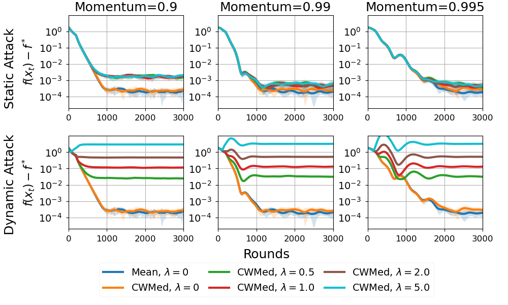
Figure 1: Optimality gap ($f(x_{t})-f^{*}$) under static (top) and dynamic (bottom) attacks across various momentum parameters and for different attack strengths ($\lambda=0,0.5,1,2,5$). The average and 95% confidence interval are presented over $20$ random seeds.

This implies the following recursion for the bias of worker $i$,

$$b_{t,i}=(1-\alpha)b_{t-1,i}+\alpha v_{t}\cdot\mathbbm{1}\left\{t\mod\frac{1}{\alpha}\in\left[\frac{i-1}{3\alpha}+1,\frac{i}{3\alpha}\right]\right\}\;.$$

Let $v\in{\mathbb{R}}^{d}$ be some fixed vector. By carefully choosing $v_{t}$, as we describe next, we ensure that $b_{t,i}=v$ for all rounds $t$ under which worker $i$ is Byzantine. Note that $b_{1,1}=v_{1}$, and $b_{1,2}=b_{1,3}=0$. We distinguish between the first epoch and the following ones. For the first epoch, i.e., $t\in\left[1/\alpha\right]$, we choose:

$$v_{t}=v\cdot\begin{cases}1/\alpha,&t\in\left\{\frac{1}{3\alpha}+1,\frac{2}{3\alpha}+1\right\}\\ 1,&\text{otherwise}.\end{cases}$$

For the subsequent epochs, i.e., $t\in\left[\frac{1}{\alpha}+1,T\right]$, we choose:

$$v_{t}=v\cdot\begin{cases}\left(1-(1-\alpha)^{2/3\alpha}\right)/\alpha,&t\mod\frac{1}{\alpha}=1\\ 1,&\text{otherwise}.\end{cases}$$

The following lemma establishes that all worker momentums are sufficiently biased under this attack.

Lemma E.1.

Given the above attack, for any $t$ starting from the second epoch, the following holds for $i=1,2,3$:

$$\tilde{m}_{t,i}=m_{t,i}+\theta_{t,i}v\;,$$

where $\theta_{t,i}\in\left[\theta_{\min},1\right]$ for each $i$ and for all $t>1/\alpha$. Here, $\theta_{\min}\coloneqq\left(\frac{5}{6}\right)^{4}>0.48$.

Proof.

Let us examine the bias dynamics of the first worker under the described attack.

In the first third of each epoch, namely, for $t\mod\frac{1}{\alpha}\in\left[\frac{1}{3\alpha}+1,\frac{1}{3\alpha}\right]$, we have a fixed bias of $b_{t,1}=v$. For the remaining two thirds, we have an exponential bias decay, where $b_{t,1}=\theta_{t,1}v$ for $\theta_{t,1}\coloneqq(1-\alpha)^{\left(t-\frac{1}{3\alpha}\right)\mod\frac{1}{\alpha}}$. Since $\beta^{t}$ is decreasing with $t$ for $\beta<1$, the coefficients sequence $\theta_{t,i}$ obtains its minimum at the end of each epoch, when $t\mod\frac{1}{\alpha}=0$, given by $(1-\alpha)^{2/3\alpha}$. For $\alpha\leq 1/6$, it holds that $(1-\alpha)^{2/3\alpha}\geq\left(\frac{5}{6}\right)^{4}\coloneqq\theta_{\min}$. Since $\theta_{t,2}$ and $\theta_{t,3}$ are simply a shift of $\theta_{t,1}$ by $1/3\alpha$ and $2/3\alpha$ rounds, respectively, they satisfy the same bounds. ∎

Given the above bias statement, any robust aggregation rule has no ability to infer an unbiased momentum path, and it would arbitrarily fail as $v$ is unbounded.

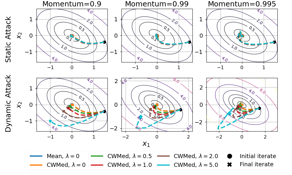
Figure 2: Optimization trajectories under static (top) and dynamic (bottom) attacks for a range of momentum parameters and for different attack strengths ($\lambda=0,0.5,1,2,5$). Note that under the dynamic attack, the algorithm converges to a sub-optimal solution.

We provide an empirical evidence to demonstrate our observation using a simple 2D quadratic example. Consider the function $f(x)=\frac{1}{2}x^{T}Ax$ with $x\in{\mathbb{R}}^{2}$ and $A$ is the matrix $\begin{bmatrix}2&1\\ 1&2\end{bmatrix}$. In our attack setup, each worker ($i=1,2,3$) employs momentum-SGD. The honest gradient oracle for each worker is defined as $g_{t,i}=\nabla_{t}+n_{t,i}$, where $n_{t,i}\overset{i.i.d}{\sim}\mathcal{N}(0,\sigma^{2}I)$ with $\sigma=0.5$. We set the attack vector to $v=\lambda\cdot\begin{bmatrix}1&1\end{bmatrix}^{\top}$, and examine various values of $\lambda\in\left\{0,0.5,1,2,5\right\}$ ($\lambda=0$ corresponds to the Byzantine-free setting). At the server level, we process the worker-momentums using either simple averaging (Mean) or coordinate-wise median (CWMed). The aggregated momentum $\widehat{m}_{t}$ is then used in the update rule: $x_{t+1}=x_{t}-\eta\widehat{m}_{t}$ with a learning rate $\eta=5\cdot 10^{-3}$ over $T=3000$ rounds. We experiment with various momentum parameters $\beta$ from $\left\{0.9,0.99,0.995\right\}$, corresponding to $\alpha$ values of $\left\{0.1.0.01,0.005\right\}$, and repeat each experiment with $20$ different random seeds. Note that these values correspond to $\lvert\tau_{c}\rvert=999,90,45$ rounds with Byzantine identity changes. Additionally, we include a ’static attack’ scenario where only the first worker is consistently Byzantine, using $\tilde{g}_{t,1}=g_{t,1}+v$ throughout all rounds.

In Figure 1, we illustrate the optimality gap during the training process. Notably, in the presence of a dynamic attack (where $\lambda>0$), we observe that the error plateaus at a sub-optimal level for all values of the momentum parameter. Furthermore, there is a clear trend that shows an increase in the final error magnitude in direct proportion to the strength of the attack (as $\lambda$ increases). This trend is distinct from what we observe under a static attack, where such a correlation between the attack strength and final error is not apparent.

Correspondingly, in Figure 2, we present a representative example showcasing the optimization paths under the influence of the static and dynamic attacks, with various momentum parameters. The trajectories visibly diverge towards sub-optimal points under dynamic attacks, with the divergence growing as the attack strength, i.e., $\lambda$, is increased. In contrast, the static attack scenarios reveal paths that remain relatively stable despite changes in attack strength. This visual illustration underscores the possible failure of the worker-momentum approach under dynamic Byzantine attack.

Appendix F Properties of the MFM Aggregator

In this section, we establish the properties of the MFM aggregator, crucial for our analysis of Section 5. Additionally, in Section F.1, we demonstrate that MFM does not meet the $(\delta,\kappa)$-robustness criteria.

We assume the gradient noise is bounded (2.2) and consider the MFM aggregator with inputs $\macc@depth\char 1\relax\frozen@everymath{\macc@group}\macc@set@skewchar\macc@nested@a 111{g}_{1}^{N},\ldots,\macc@depth\char 1\relax\frozen@everymath{\macc@group}\macc@set@skewchar\macc@nested@a 111{g}_{m}^{N}$ as in Lemma 3.4 and threshold parameter set to $\mathcal{T}_{p}^{N}=2C_{p}\mathcal{V}/\sqrt{N}$, where $C_{p}\coloneqq\sqrt{8\log\!\left(2m/p\right)}$.

Initially, we introduce the following event, under which we derive valuable insights regarding Algorithm 3.

$$\mathcal{B}=\left\{\forall i\in\mathcal{G}:\left\|\macc@depth\char 1\relax\frozen@everymath{\macc@group}\macc@set@skewchar\macc@nested@a 111{g}_{i}^{N}-\nabla f(x)\right\|\leq\frac{\mathcal{T}_{p}^{N}}{4}=\mathcal{V}\sqrt{\frac{2\log{\left(2m/p\right)}}{N}}\right\}\;.$$ (24)

Here, we analyze Algorithm 3 assuming the honest workers are fixed when computing mini-batches.

First, we show that $\mathcal{B}$ is satisfied with high probability.

Lemma F.1.

For every $x\in{\mathbb{R}}$, it holds that $\mathbb{P}(\mathcal{B})\geq 1-p$.

Proof.

Since for every $i\in\mathcal{G}$, $\macc@depth\char 1\relax\frozen@everymath{\macc@group}\macc@set@skewchar\macc@nested@a 111{g}_{i}^{N}=\frac{1}{N}\sum_{n=1}^{N}{\nabla F(x;\xi_{i}^{n})}$, where $\left\|\nabla F(x;\xi_{i}^{n})-\nabla f(x)\right\|\leq\mathcal{V}$, utilizing Lemma I.1 implies that with probability at least $1-\tilde{p}$, we have $\left\|\macc@depth\char 1\relax\frozen@everymath{\macc@group}\macc@set@skewchar\macc@nested@a 111{g}_{i}^{N}-\nabla f(x)\right\|\leq\mathcal{V}\sqrt{\frac{2\log\left(2/\tilde{p}\right)}{N}}$. Employing the union bound and using $\lvert\mathcal{G}\rvert\leq m$ establishes the result. ∎

Next, we establish some results assuming $\mathcal{B}$ holds.

Lemma F.2.

Under the event $\mathcal{B}$, the following holds:

1. The set $\mathcal{M}$ is not empty.

2. $\mathcal{G}\subseteq\widehat{\mathcal{G}}$.

3. For every $i\in\widehat{\mathcal{G}}$, we have $\left\|\macc@depth\char 1\relax\frozen@everymath{\macc@group}\macc@set@skewchar\macc@nested@a 111{g}_{i}^{N}-\nabla f(x)\right\|\leq 2\mathcal{T}_{p}^{N}$.

Proof.

Following the proof of Claim 3.4 in Alistarh et al. (2018): under the event $\mathcal{B}$, for every $i,j\in\mathcal{G}$, we have by the triangle inequality that $\left\|\macc@depth\char 1\relax\frozen@everymath{\macc@group}\macc@set@skewchar\macc@nested@a 111{g}_{i}^{N}-\macc@depth\char 1\relax\frozen@everymath{\macc@group}\macc@set@skewchar\macc@nested@a 111{g}_{j}^{N}\right\|\leq\left\|\macc@depth\char 1\relax\frozen@everymath{\macc@group}\macc@set@skewchar\macc@nested@a 111{g}_{i}^{N}-\nabla f(x)\right\|+\left\|\macc@depth\char 1\relax\frozen@everymath{\macc@group}\macc@set@skewchar\macc@nested@a 111{g}_{j}^{N}-\nabla f(x)\right\|\leq\nicefrac{{\mathcal{T}_{p}^{N}}}{{2}}$. Since $\delta<\nicefrac{{1}}{{2}}$, every $i\in\mathcal{G}$ is also in $\mathcal{M}$, namely, $\mathcal{G}\subseteq\mathcal{M}$, which concludes the first part.

For the second and third parts, we first show that $\left\|g_{\text{med}}-\nabla f(x)\right\|\leq\nicefrac{{3\mathcal{T}_{p}^{N}}}{{4}}$; assuming $\left\|g_{\text{med}}-\nabla f(x)\right\|>\nicefrac{{3\mathcal{T}_{p}^{N}}}{{4}}$, we get by the triangle inequality that $\left\|g_{\text{med}}-\macc@depth\char 1\relax\frozen@everymath{\macc@group}\macc@set@skewchar\macc@nested@a 111{g}_{i}^{N}\right\|>\nicefrac{{\mathcal{T}_{p}^{N}}}{{2}}$ for every $i\in\mathcal{G}$, thus contradicting the definition of $g_{\text{med}}$ (chosen from $\mathcal{M}$) as $\lvert\mathcal{G}\rvert>\nicefrac{{m}}{{2}}$.

To prove the second part, fix some $i\in\mathcal{G}$. By the triangle inequality: $\left\|\macc@depth\char 1\relax\frozen@everymath{\macc@group}\macc@set@skewchar\macc@nested@a 111{g}_{i}^{N}-g_{\text{med}}\right\|\leq\left\|\macc@depth\char 1\relax\frozen@everymath{\macc@group}\macc@set@skewchar\macc@nested@a 111{g}_{i}^{N}-\nabla f(x)\right\|+\left\|g_{\text{med}}-\nabla f(x)\right\|\leq\nicefrac{{\mathcal{T}_{p}^{N}}}{{4}}+\nicefrac{{3\mathcal{T}_{p}^{N}}}{{4}}=\mathcal{T}_{p}^{N}$, where the bound on $\left\|\macc@depth\char 1\relax\frozen@everymath{\macc@group}\macc@set@skewchar\macc@nested@a 111{g}_{i}^{N}-\nabla f(x)\right\|$ follows from the definition of $\mathcal{B}$. This bound implies that $i\in\widehat{\mathcal{G}}$ as well, concluding the second part.

Finally, note that for any $i\in\widehat{\mathcal{G}}$, the triangle inequality implies $\left\|\macc@depth\char 1\relax\frozen@everymath{\macc@group}\macc@set@skewchar\macc@nested@a 111{g}_{i}^{N}-\nabla f(x)\right\|\leq\left\|\macc@depth\char 1\relax\frozen@everymath{\macc@group}\macc@set@skewchar\macc@nested@a 111{g}_{i}^{N}-g_{\text{med}}\right\|+\left\|g_{\text{med}}-\nabla f(x)\right\|\leq\mathcal{T}_{p}^{N}+\nicefrac{{3\mathcal{T}_{p}^{N}}}{{4}}\leq 2\mathcal{T}_{p}^{N}$, where $\left\|\macc@depth\char 1\relax\frozen@everymath{\macc@group}\macc@set@skewchar\macc@nested@a 111{g}_{i}^{N}-g_{\text{med}}\right\|\leq\mathcal{T}_{p}^{N}$ holds for any $i\in\widehat{\mathcal{G}}$ as established in the previous part. ∎

With these insights, we now prove Lemma F.3, which, similarly to Lemma D.1, provides deterministic and high-probability bounds on the aggregation error.

Lemma F.3.

Consider the setting in Lemma D.1 and let $\widehat{g}^{N}\leftarrow\text{MFM}(\macc@depth\char 1\relax\frozen@everymath{\macc@group}\macc@set@skewchar\macc@nested@a 111{g}_{1}^{N},\ldots,\macc@depth\char 1\relax\frozen@everymath{\macc@group}\macc@set@skewchar\macc@nested@a 111{g}_{m}^{N};\mathcal{T}_{p}^{N})$ be the output of Algorithm 3 with $\mathcal{T}_{p}^{N}\coloneqq 2C_{p}\mathcal{V}/\sqrt{N}$, where $C_{p}\coloneqq\sqrt{8\log\!\left(2m/p\right)}$. Then,

1. $\left\|\widehat{g}^{N}-\nabla f(x)\right\|^{2}\leq\frac{9}{2}(\mathcal{T}_{p}^{N})^{2}+2\mathcal{V}^{2}+\left\|\nabla f(x)\right\|^{2}\leq 20C_{p}^{2}\mathcal{V}^{2}+\left\|\nabla f(x)\right\|^{2}$.

2. With probability at least $1-p$,

   $$\left\|\widehat{g}^{N}-\nabla f(x)\right\|^{2}\leq\frac{2C_{p}^{2}\mathcal{V}^{2}}{N}\left(\frac{1}{m}+128\delta^{2}\right)\;.$$

Proof.

Denote: $\nabla\coloneqq\nabla f(x)$. To prove the first part, we consider two cases: when $\mathcal{M}$ is either empty or non-empty. If $\mathcal{M}=\emptyset$, then $\widehat{g}^{N}=0$, leading to $\left\|\widehat{g}^{N}-\nabla\right\|^{2}=\left\|\nabla\right\|^{2}$. In the case where $\mathcal{M}$ is non-empty, the triangle inequality implies that

$$\left\|\widehat{g}^{N}-\nabla\right\|=\left\|\frac{1}{\lvert\widehat{\mathcal{G}}\rvert}\sum_{i\in\widehat{\mathcal{G}}}{\left(\macc@depth\char 1\relax\frozen@everymath{\macc@group}\macc@set@skewchar\macc@nested@a 111{g}_{i}^{N}-\nabla\right)}\right\|\leq\frac{1}{\lvert\widehat{\mathcal{G}}\rvert}\sum_{i\in\widehat{\mathcal{G}}}{\left\|g_{i}^{N}-\nabla\right\|}\;.$$

Since $g_{\text{med}}=\macc@depth\char 1\relax\frozen@everymath{\macc@group}\macc@set@skewchar\macc@nested@a 111{g}_{i}^{N}$ for some $i\in\mathcal{M}$, by the definition of $\mathcal{M}$, there are more than $\nicefrac{{m}}{{2}}$ machines whose distance from $g_{\text{med}}$ is bounded by $\nicefrac{{\mathcal{T}_{p}^{N}}}{{2}}$. Since there are at most $\delta m<\nicefrac{{m}}{{2}}$ Byzantine workers, it implies that at least one of the above workers is good; denote one such worker by $\ell\in\mathcal{G}$. Thus, for every $i\in\widehat{\mathcal{G}}$ we can bound,

$$\left\|\macc@depth\char 1\relax\frozen@everymath{\macc@group}\macc@set@skewchar\macc@nested@a 111{g}_{i}^{N}-\nabla\right\| \leq\underbrace{\left\|\macc@depth\char 1\relax\frozen@everymath{\macc@group}\macc@set@skewchar\macc@nested@a 111{g}_{i}^{N}-g_{\text{med}}\right\|}_{\leq\mathcal{T}_{p}^{N}}+\underbrace{\left\|g_{\text{med}}-\macc@depth\char 1\relax\frozen@everymath{\macc@group}\macc@set@skewchar\macc@nested@a 111{g}_{\ell}^{N}\right\|}_{\leq\nicefrac{{\mathcal{T}_{p}^{N}}}{{2}}}+\underbrace{\left\|\macc@depth\char 1\relax\frozen@everymath{\macc@group}\macc@set@skewchar\macc@nested@a 111{g}_{\ell}^{N}-\nabla\right\|}_{\leq\mathcal{V}}\leq\frac{3\mathcal{T}_{p}^{N}}{2}+\mathcal{V}\;,$$

where the first bound is by the definition of $\widehat{\mathcal{G}}$, the second bound is a consequence of the chosen $\ell$ (and the definition of $g_{\text{med}}$), and the final bound is trivial for any good worker. Since this bound holds for any $i\in\widehat{\mathcal{G}}$, it also holds for $\widehat{g}^{N}$. Thus, using $(a+b)^{2}\leq 2a^{2}+2b^{2}$, we have

$$\left\|\widehat{g}^{N}-\nabla\right\|^{2} \leq 2\left(\frac{9}{4}(\mathcal{T}_{p}^{N})^{2}+\mathcal{V}^{2}\right)=\frac{9}{2}(\mathcal{T}_{p}^{N})^{2}+2\mathcal{V}^{2}\;.$$

Overall, in any case, we have that

$$\left\|\widehat{g}^{N}-\nabla\right\|^{2}\leq\max\left\{\left\|\nabla\right\|^{2},\frac{9}{2}(\mathcal{T}_{p}^{N})^{2}+2\mathcal{V}^{2}\right\} \leq\frac{9}{2}(\mathcal{T}_{p}^{N})^{2}+2\mathcal{V}^{2}+\left\|\nabla\right\|^{2}$$

$$=\frac{9}{2}\cdot\frac{4C_{p}^{2}\mathcal{V}^{2}}{N}+2\mathcal{V}^{2}+\left\|\nabla\right\|^{2}$$

$$\leq 20C_{p}^{2}\mathcal{V}^{2}+\left\|\nabla\right\|^{2}\;,$$

where we used $C_{p}^{2}\geq 1$. This concludes the first part.

For the second part, we denote the average of honest workers by ${\macc@depth\char 1\relax\frozen@everymath{\macc@group}\macc@set@skewchar\macc@nested@a 111{g}}^{N}\coloneqq\frac{1}{\lvert\mathcal{G}\rvert}\sum_{i\in\mathcal{G}}{\macc@depth\char 1\relax\frozen@everymath{\macc@group}\macc@set@skewchar\macc@nested@a 111{g}_{i}^{N}}$ and define the following events:

$$\widehat{\mathcal{C}}\coloneqq\left\{\left\|\widehat{g}^{N}-\nabla\right\|\leq 2\mathcal{V}\sqrt{\frac{\log{\left(2/p\right)}}{mN}}+4\delta\mathcal{T}_{p}^{N}\right\},$$

$$\macc@depth\char 1\relax\frozen@everymath{\macc@group}\macc@set@skewchar\macc@nested@a 111{}\coloneqq\left\{\left\|{\macc@depth\char 1\relax\frozen@everymath{\macc@group}\macc@set@skewchar\macc@nested@a 111{g}}^{N}-\nabla\right\|\leq 2\mathcal{V}\sqrt{\frac{\log{\left(2/p\right)}}{mN}}\right\}\;.$$

Our objective is to establish that $\widehat{\mathcal{C}}$ holds with probability at least $1-2p$. Recall that under the event $\mathcal{B}$ (Equation 24), the set $\mathcal{M}$ is non-empty (item 1 of Lemma F.2), implying $\widehat{g}^{N}=\frac{1}{\lvert\widehat{\mathcal{G}}\rvert}\sum_{i\in\widehat{\mathcal{G}}}{\macc@depth\char 1\relax\frozen@everymath{\macc@group}\macc@set@skewchar\macc@nested@a 111{g}_{i}^{N}}$, and $\mathcal{G}\subseteq\widehat{\mathcal{G}}$. Hence, under the event $\mathcal{B}$, we have that

$$\left\|\widehat{g}^{N}-\nabla\right\|=\left\|\frac{1}{\lvert\widehat{\mathcal{G}}\rvert}\sum_{i\in\widehat{\mathcal{G}}}{({\macc@depth\char 1\relax\frozen@everymath{\macc@group}\macc@set@skewchar\macc@nested@a 111{g}_{i}^{N}}-\nabla})\right\| =\left\|\frac{1}{\lvert\widehat{\mathcal{G}}\rvert}\sum_{i\in\mathcal{G}}{(\macc@depth\char 1\relax\frozen@everymath{\macc@group}\macc@set@skewchar\macc@nested@a 111{g}_{i}^{N}-\nabla)}+\frac{1}{\lvert\widehat{\mathcal{G}}\rvert}\sum_{i\in\widehat{\mathcal{G}}\setminus\mathcal{G}}{(\macc@depth\char 1\relax\frozen@everymath{\macc@group}\macc@set@skewchar\macc@nested@a 111{g}_{i}^{N}-\nabla)}\right\|$$

$$\leq\frac{\lvert\mathcal{G}\rvert}{\lvert\widehat{\mathcal{G}}\rvert}\left\|{\macc@depth\char 1\relax\frozen@everymath{\macc@group}\macc@set@skewchar\macc@nested@a 111{g}}^{N}-\nabla\right\|+\frac{1}{\lvert\widehat{\mathcal{G}}\rvert}\sum_{i\in\widehat{\mathcal{G}}\setminus\mathcal{G}}{\left\|\macc@depth\char 1\relax\frozen@everymath{\macc@group}\macc@set@skewchar\macc@nested@a 111{g}_{i}^{N}-\nabla\right\|}$$

$$\leq\left\|{\macc@depth\char 1\relax\frozen@everymath{\macc@group}\macc@set@skewchar\macc@nested@a 111{g}}^{N}-\nabla\right\|+\frac{2}{m}\lvert\widehat{\mathcal{G}}\setminus\mathcal{G}\rvert\cdot 2\mathcal{T}_{p}^{N}$$

$$\leq\left\|{\macc@depth\char 1\relax\frozen@everymath{\macc@group}\macc@set@skewchar\macc@nested@a 111{g}}^{N}-\nabla\right\|+4\delta\mathcal{T}_{p}^{N}\;,$$ (25)

where the first inequality follows from the triangle inequality and the following relation: $\sum_{i\in\mathcal{G}}{(\macc@depth\char 1\relax\frozen@everymath{\macc@group}\macc@set@skewchar\macc@nested@a 111{g}_{i}^{N}-\nabla)}=\lvert\mathcal{G}\rvert({\macc@depth\char 1\relax\frozen@everymath{\macc@group}\macc@set@skewchar\macc@nested@a 111{g}}^{N}-\nabla)$; the second inequality is due to $\lvert\widehat{\mathcal{G}}\rvert\geq\lvert\mathcal{G}\rvert\geq\nicefrac{{m}}{{2}}$ and item 3 of Lemma F.2, namely, $\lVert{\macc@depth\char 1\relax\frozen@everymath{\macc@group}\macc@set@skewchar\macc@nested@a 111{g}_{i}^{N}-\nabla\rVert}\leq 2\mathcal{T}_{p}^{N}$ for all $i\in\widehat{\mathcal{G}}$; and the last inequality follows from $\lvert\widehat{\mathcal{G}}\setminus\mathcal{G}\rvert\leq\lvert\left[m\right]\setminus\mathcal{G}\rvert=\delta m$.

Based on Appendix F, we infer that, under the event $\mathcal{B}$, if $\macc@depth\char 1\relax\frozen@everymath{\macc@group}\macc@set@skewchar\macc@nested@a 111{}$ occurs, then so does $\widehat{\mathcal{C}}$, implying $\mathbb{P}(\widehat{\mathcal{C}}|\mathcal{B})\geq\mathbb{P}(\macc@depth\char 1\relax\frozen@everymath{\macc@group}\macc@set@skewchar\macc@nested@a 111{}|\mathcal{B})$. Furthermore, we have by Lemma F.1 that $\mathbb{P}(\mathcal{B})\geq 1-p>0$. Combining these properties and utilizing Lemma I.6 yields:

$$\mathbb{P}(\widehat{\mathcal{C}})\geq\mathbb{P}(\macc@depth\char 1\relax\frozen@everymath{\macc@group}\macc@set@skewchar\macc@nested@a 111{})-\mathbb{P}(\mathcal{B}^{c})\geq\mathbb{P}(\macc@depth\char 1\relax\frozen@everymath{\macc@group}\macc@set@skewchar\macc@nested@a 111{})-p\;.$$ (26)

By Lemma I.1, it holds with probability at least $1-p$ that

$$\left\|{\macc@depth\char 1\relax\frozen@everymath{\macc@group}\macc@set@skewchar\macc@nested@a 111{g}}^{N}-\nabla\right\|=\frac{1}{\lvert\mathcal{G}\rvert N}\left\|\sum_{i\in\mathcal{G}}{\sum_{n\in\left[N\right]}{\left(\nabla F(x;\xi_{i}^{n})-\nabla\right)}}\right\|\leq\mathcal{V}\sqrt{\frac{2\log{\left(2/p\right)}}{\lvert\mathcal{G}\rvert N}}\leq 2\mathcal{V}\sqrt{\frac{\log{\left(2/p\right)}}{mN}}\;.$$

In other words, $\mathbb{P}(\macc@depth\char 1\relax\frozen@everymath{\macc@group}\macc@set@skewchar\macc@nested@a 111{})\geq 1-p$, indicating, as per Equation 26, that with a probability of at least $1-2p$,

$$\left\|\widehat{g}^{N}-\nabla\right\|\leq 2\mathcal{V}\sqrt{\frac{\log{\left(2/p\right)}}{mN}}+4\delta\mathcal{T}_{p}^{N} =2\mathcal{V}\sqrt{\frac{\log{\left(2/p\right)}}{mN}}+16\delta\mathcal{V}\sqrt{\frac{2\log\left(2m/p\right)}{N}}$$

$$=2\mathcal{V}\sqrt{\frac{\log\left(2m/p\right)}{N}}\left(\frac{1}{\sqrt{m}}+8\sqrt{2}\delta\right)\;.$$

This result finally implies that with probability at least $1-p$,

$$\left\|\widehat{g}^{N}-\nabla\right\|^{2}\leq\frac{4\mathcal{V}^{2}\log\left(4m/p\right)}{N}\left(\frac{1}{\sqrt{m}}+8\sqrt{2}\delta\right)^{2} \leq\frac{8\mathcal{V}^{2}\log\left(4m/p\right)}{N}\left(\frac{1}{m}+128\delta^{2}\right)$$

$$\leq\frac{2C_{p}^{2}\mathcal{V}^{2}}{N}\left(\frac{1}{m}+128\delta^{2}\right)\;,$$

where we used $(a+b)^{2}\leq 2(a^{2}+b^{2})$ and $8\log\left(4m/p\right)\leq 16\log\left(4m/p\right)=2C_{p}^{2}$. ∎

Combining the bounds established in Lemma F.3, we can derive an upper bound on the expected (squared) aggregation error, mirroring Corollary D.2.

Corollary F.4 (MSE of Aggregated Gradients).

Consider the setting in Lemma D.1. In addition, let $\widehat{g}^{N}\leftarrow\text{MFM}(\macc@depth\char 1\relax\frozen@everymath{\macc@group}\macc@set@skewchar\macc@nested@a 111{g}_{1}^{N},\ldots,\macc@depth\char 1\relax\frozen@everymath{\macc@group}\macc@set@skewchar\macc@nested@a 111{g}_{m}^{N};\mathcal{T}^{N})$ be the output of Algorithm 3 with threshold parameter $\mathcal{T}^{N}\coloneqq 2C\mathcal{V}/\sqrt{N}=4\mathcal{V}\sqrt{2\log{\left(16m^{2}T\right)}/N}$, and assume that $N\leq T$. Then,

$$\mathbb{E}\!\left\|\widehat{g}^{N}-\nabla f(x)\right\|^{2}\leq\frac{\tilde{C}^{2}\mathcal{V}^{2}\tilde{\gamma}}{N}+\frac{\left\|\nabla f(x)\right\|^{2}}{8mT}\;,$$

where $\tilde{C}^{2}\coloneqq 8C^{2}=64\log\!\left(16m^{2}T\right)$ and $\tilde{\gamma}\coloneqq\frac{1}{m}+32\delta^{2}$.

Proof.

Utilizing the previous lemma, we have with probability at least $1-\frac{1}{8mT}$,

$$\left\|\widehat{g}^{N}-\nabla f(x)\right\|^{2}\leq\frac{2C^{2}\mathcal{V}^{2}}{N}\left(\frac{1}{m}+128\delta^{2}\right)\;.$$

Additionally, we always have that

$$\left\|\widehat{g}^{N}-\nabla f(x)\right\|^{2}\leq 20C^{2}\mathcal{V}^{2}+\left\|\nabla f(x)\right\|^{2}\;.$$

Thus, by the law of total expectation, we get

$$\mathbb{E}\!\left\|\widehat{g}^{N}-\nabla f(x)\right\|^{2} \leq\frac{2C^{2}\mathcal{V}^{2}}{N}\left(\frac{1}{m}+128\delta^{2}\right)+\left(20C^{2}\mathcal{V}^{2}+\left\|\nabla f(x)\right\|^{2}\right)\cdot\frac{1}{8mT}$$

$$=\frac{2C^{2}\mathcal{V}^{2}}{N}\left(\frac{1}{m}+128\delta^{2}\right)+\frac{5C^{2}\mathcal{V}^{2}}{2mT}+\frac{\left\|\nabla f(x)\right\|^{2}}{8mT}$$

$$=\frac{C^{2}\mathcal{V}^{2}}{N}\left(\frac{9}{2m}+256\delta^{2}\right)+\frac{\left\|\nabla f(x)\right\|^{2}}{8mT}$$

$$\leq\frac{8C^{2}\mathcal{V}^{2}}{N}\left(\frac{1}{m}+32\delta^{2}\right)+\frac{\left\|\nabla f(x)\right\|^{2}}{8mT}$$

$$=\frac{\tilde{C}^{2}\mathcal{V}^{2}\tilde{\gamma}}{N}+\frac{\left\|\nabla f(x)\right\|^{2}}{8mT}\;,$$

where the second inequality follows from the assumption that $N\leq T$. ∎

The bound in Corollary F.4 closely resembles that in Corollary D.2, differing by an additional factor of $\frac{\left\|\nabla f(x)\right\|^{2}}{8mT}$. This variation stems from the specific structure of the MFM aggregator, specifically due to the rare event where the set $\mathcal{M}$ is empty, leading to an output of $\widehat{g}=0$.

F.1 MFM is not $(\delta,\kappa)$-robust

Consider Algorithm 3 with a threshold $\mathcal{T}>0$, and let $x\in{\mathbb{R}}^{d}$. Suppose every honest worker $i\in\mathcal{G}$ provides the true gradient, $g_{i}=\nabla f(x)$, while every Byzantine worker submits $g_{i}=\nabla f(x)+\frac{3}{4}\mathcal{T}v$, for some $v\in{\mathbb{R}}^{d}$ with $\left\|v\right\|=1$. In this case, $\mathcal{M}$ is not empty as $\mathcal{M}=\mathcal{G}$. Since all vectors are within $\frac{3}{4}\mathcal{T}$ of each other, $\widehat{\mathcal{G}}$ contains all workers. Consequently, the aggregated gradient, $\widehat{g}$, is given by $\nabla f(x)+\frac{3}{4}\mathcal{T}\delta v$. Denoting the average of honest workers by $\macc@depth\char 1\relax\frozen@everymath{\macc@group}\macc@set@skewchar\macc@nested@a 111{g}=\frac{1}{\lvert\mathcal{G}\rvert}\sum_{i\in\mathcal{G}}{g_{i}}=\nabla f(x)$, the above implies a nonzero aggregation error $\left\|\widehat{g}-\macc@depth\char 1\relax\frozen@everymath{\macc@group}\macc@set@skewchar\macc@nested@a 111{g}\right\|$, while the ‘variance’ among honest workers, $\frac{1}{\lvert\mathcal{G}\rvert}\sum_{i\in\mathcal{G}}{\left\|g_{i}-\macc@depth\char 1\relax\frozen@everymath{\macc@group}\macc@set@skewchar\macc@nested@a 111{g}\right\|^{2}}$, remains zero. This scenario fails to satisfy Definition 3.3.

Appendix G AdaGrad with Biased Gradients

Consider the AdaGrad-Norm (Levy, 2017; Ward et al., 2020; Faw et al., 2022) (also known as AdaSGD, Attia and Koren, 2023) update rule, defined for some parameter $\eta_{0}>0$ as follows:

$$x_{t+1}=\Pi_{\mathcal{K}}(x_{t}-\eta_{t}g_{t}),\quad\eta_{t}=\frac{\eta_{0}}{\sqrt{\sum_{s=1}^{t}{\left\|g_{s}\right\|^{2}}}}\;,$$ (AdaGrad-Norm)

where $g_{t}$ has bias $b_{t}\coloneqq\mathbb{E}[g_{t}-\nabla f(x_{t})|x_{t}]$ and variance $V_{t}^{2}\coloneqq\mathbb{E}[\left\|g_{t}-\mathbb{E}g_{t}\right\|^{2}|x_{t}]$.

In Sections G.1 and G.2, convergence bounds for (AdaGrad-Norm) are deduced for convex and non-convex objectives, respectively.

G.1 Convex Analysis

We commence with a lemma that establishes a second-order bound on the linearized regret of (AdaGrad-Norm), essential in our convex analysis. The proof is included for completeness.

Lemma G.1 (Levy, 2017, Theorem 1.1).

Suppose 2.3 holds, i.e., the domain $\mathcal{K}$ is bounded with diameter $D\coloneqq\max_{x,y\in\mathcal{K}}{\left\|x-y\right\|}$ and consider (AdaGrad-Norm). Then, for every $u\in\mathcal{K}$, the iterates $x_{1},\ldots,x_{T}$ satisfy:

$$\sum_{t=1}^{T}{g_{t}^{\top}(x_{t}-u)}\leq\left(\frac{D^{2}}{2\eta_{0}}+\eta_{0}\right)\sqrt{\sum_{t=1}^{T}{\left\|g_{t}\right\|^{2}}}\;.$$

Proof.

For every $u\in\mathcal{K}$, we have that

$$\left\|x_{t+1}-u\right\|^{2} \leq\left\|x_{t}-u\right\|^{2}-2\eta_{t}g_{t}^{\top}(x_{t}-u)+\eta^{2}\left\|g_{t}\right\|^{2}\;.$$

Rearranging terms, we get:

$$g_{t}^{\top}(x_{t}-u) \leq\frac{\left\|x_{t}-u\right\|^{2}-\left\|x_{t+1}-u\right\|^{2}}{2\eta_{t}}+\frac{\eta_{t}}{2}\left\|g_{t}\right\|^{2}\;.$$

Summing over $t\in\left[T\right]$, we then obtain:

$$\sum_{t=1}^{T}{g_{t}^{\top}(x_{t}-u)} \leq\frac{\left\|x_{1}-u\right\|^{2}}{2\eta_{1}}+\sum_{t=2}^{T}{\frac{\left\|x_{t}-u\right\|^{2}}{2}\left(\frac{1}{\eta_{t}}-\frac{1}{\eta_{t-1}}\right)}+\frac{1}{2}\sum_{t=1}^{T}{\eta_{t}\left\|g_{t}\right\|^{2}}$$

$$\leq\frac{D^{2}}{2}\left(\frac{1}{\eta_{1}}+\sum_{t=2}^{T}{\left(\frac{1}{\eta_{t}}-\frac{1}{\eta_{t-1}}\right)}\right)+\frac{\eta_{0}}{2}\sum_{t=1}^{T}{\frac{\left\|g_{t}\right\|^{2}}{\sqrt{\sum_{s=1}^{t}{\left\|g_{s}\right\|^{2}}}}}$$

$$=\frac{D^{2}}{2\eta_{T}}+\frac{\eta_{0}}{2}\sum_{t=1}^{T}{\frac{\left\|g_{t}\right\|^{2}}{\sqrt{\sum_{s=1}^{t}{\left\|g_{s}\right\|^{2}}}}}$$

$$\leq\frac{D^{2}}{2\eta_{0}}\sqrt{\sum_{t=1}^{T}{\left\|g_{t}\right\|^{2}}}+\eta_{0}\sqrt{\sum_{t=1}^{T}{\left\|g_{t}\right\|^{2}}}$$

$$=\left(\frac{D^{2}}{2\eta_{0}}+\eta_{0}\right)\sqrt{\sum_{t=1}^{T}{\left\|g_{t}\right\|^{2}}}\;,$$

where the second inequality uses $\left\|x_{t}-u\right\|^{2}\leq D^{2}$ for every $t\in\left[T\right]$ and $\eta_{t}\leq\eta_{t-1}$, and the final inequality stems from Lemma I.4. ∎

We now establish a regret bound for AdaGrad-Norm.

Lemma G.2.

Assume $f$ is convex. Under 2.3, the iterates of (AdaGrad-Norm) satisfy:

$$\mathbb{E}\mathcal{R}_{T}\leq D\sqrt{2\sum_{t\in\left[T\right]}{\mathbb{E}V_{t}^{2}}}+2D\sqrt{\sum_{t\in\left[T\right]}{\mathbb{E}\!\left\|b_{t}\right\|^{2}}}+D\sum_{t\in\left[T\right]}{\mathbb{E}\!\left\|b_{t}\right\|}+2D\sqrt{\sum_{t\in\left[T\right]}{\mathbb{E}\!\left\|\nabla f(x_{t})\right\|^{2}}}\;,$$

where $\mathcal{R}_{T}\coloneqq\sum_{t\in\left[T\right]}{\left(f(x_{t})-f(x^{*})\right)}$.

Proof.

By the convexity of $f$,

$$\mathbb{E}\mathcal{R}_{T}\leq\sum_{t\in\left[T\right]}{\mathbb{E}[\nabla f(x_{t})^{\top}(x_{t}-x^{*})]}=\underbrace{\mathbb{E}\!\left[\sum_{t\in\left[T\right]}{g_{t}^{\top}(x_{t}-x^{*})}\right]}_{=(A)}+\underbrace{\sum_{t\in\left[T\right]}{\mathbb{E}[-b_{t}^{\top}(x_{t}-x^{*})]}}_{=(B)}\;.$$ (27)

Bounding $(A)$.

Utilizing Lemma G.1 with $\eta_{0}=D/\sqrt{2}$ and Jensen’s inequality, we obtain:

$$\mathbb{E}\!\left[\sum_{t\in\left[T\right]}{g_{t}^{\top}(x_{t}-x^{*})}\right] \leq D\mathbb{E}\!\left[\sqrt{2\sum_{t\in\left[T\right]}{\left\|g_{t}\right\|^{2}}}\right]\leq D\sqrt{2\sum_{t\in\left[T\right]}{\mathbb{E}\!\left\|g_{t}\right\|^{2}}}\;.$$

We can bound the second moment of $g_{t}$ as follows:

$$\mathbb{E}_{t-1}\!\left\|g_{t}\right\|^{2}=\mathbb{E}_{t-1}\!\left\|g_{t}-\mathbb{E}_{t-1}g_{t}\right\|^{2}+\left\|\mathbb{E}_{t-1}g_{t}\right\|^{2}\leq V_{t}^{2}+2\left\|b_{t}\right\|^{2}+2\left\|\nabla f(x_{t})\right\|^{2}\;,$$ (28)

where we used $\left\|a+b\right\|^{2}\leq 2\left\|a\right\|^{2}+2\left\|b\right\|^{2}$. Plugging this bound back, we get that $(A)$ is bounded as

$$\mathbb{E}\!\left[\sum_{t\in\left[T\right]}{g_{t}^{\top}(x_{t}-x^{*})}\right]\leq D\sqrt{2\sum_{t\in\left[T\right]}{\mathbb{E}V_{t}^{2}}}+2D\sqrt{\sum_{t\in\left[T\right]}{\mathbb{E}\!\left\|b_{t}\right\|^{2}}}+2D\sqrt{\sum_{t\in\left[T\right]}{\mathbb{E}\!\left\|\nabla f(x_{t})\right\|^{2}}}\;.$$

Bounding $(B)$.

By Cauchy-Schwarz inequality and 2.3,

$$\sum_{t\in\left[T\right]}{\mathbb{E}[-b_{t}^{\top}(x_{t}-x^{*})]}\leq\sum_{t\in\left[T\right]}{\mathbb{E}[\left\|b_{t}\right\|\left\|x_{t}-x^{*}\right\|]}\leq D\sum_{t\in\left[T\right]}{\mathbb{E}\!\left\|b_{t}\right\|}\;.$$

Incorporating the bounds on $(A)$ and $(B)$ into Equation 27 concludes the proof, as

$$\mathbb{E}\mathcal{R}_{T} \leq D\sqrt{2\sum_{t\in\left[T\right]}{\mathbb{E}V_{t}^{2}}}+2D\sqrt{\sum_{t\in\left[T\right]}{\mathbb{E}\!\left\|b_{t}\right\|^{2}}}+D\sum_{t\in\left[T\right]}{\mathbb{E}\!\left\|b_{t}\right\|}+2D\sqrt{\sum_{t\in\left[T\right]}{\mathbb{E}\!\left\|\nabla f(x_{t})\right\|^{2}}}\;.$$

∎

G.2 Non-Convex Analysis

The subsequent lemma establishes an upper bound on the sum of squared gradient norms when utilizing AdaGrad-Norm for bounded functions.

Lemma G.3.

Assume $f$ is bounded by $M$, i.e., $\max_{x}{\lvert f(x)\rvert}\leq M$, and consider (AdaGrad-Norm) with $\mathcal{K}={\mathbb{R}}^{d}$. The iterates $x_{1},\ldots,x_{T}$ satisfy:

$$\sum_{t=1}^{T}{\left\|\nabla f(x_{t})\right\|^{2}}\leq\left(\frac{2M}{\eta_{0}}+\eta_{0}L\right)\sqrt{\sum_{t=1}^{T}{\lVert g_{t}\rVert}^{2}}+\sum_{t=1}^{T}{\left(\nabla f(x_{t})-g_{t}\right)^{\top}\nabla f(x_{t})}\;.$$

Proof.

By the smoothness of $f$, for every $x,y\in{\mathbb{R}}^{d}$ we have that $f(y)\leq f(x)+\nabla f(x)^{\top}(y-x)+\frac{L}{2}\left\|y-x\right\|^{2}$. Plugging-in the update rule $x_{t+1}=x_{t}-\eta_{t}g_{t}$, we obtain:

$$f(x_{t+1}) \leq f(x_{t})-\eta_{t}\nabla f(x_{t})^{\top}g_{t}+\frac{L\eta_{t}^{2}}{2}\left\|g_{t}\right\|^{2}$$

$$=f(x_{t})-\eta_{t}\left\|\nabla f(x_{t})\right\|^{2}+\eta_{t}\left(\nabla f(x_{t})-g_{t}\right)^{\top}\nabla f(x_{t})+\frac{L\eta_{t}^{2}}{2}\left\|g_{t}\right\|^{2}\;.$$

Rearranging terms and dividing by $\eta_{t}$ gives:

$$\left\|\nabla f(x_{t})\right\|^{2}\leq\frac{f(x_{t})-f(x_{t+1})}{\eta_{t}}+\frac{L\eta_{t}}{2}\left\|g_{t}\right\|^{2}+\left(\nabla f(x_{t})-g_{t}\right)^{\top}\nabla f(x_{t})\;.$$

Denoting $\Delta_{t}\coloneqq f(x_{t})-f^{*}$ and $\Delta_{\max}\coloneqq\max_{t\in\left[T\right]}{f(x_{t})-f^{*}}$. Thus, the above is equivalent to

$$\left\|\nabla f(x_{t})\right\|^{2}\leq\frac{\Delta_{t}-\Delta_{t+1}}{\eta_{t}}+\frac{L\eta_{t}}{2}\left\|g_{t}\right\|^{2}+\left(\nabla f(x_{t})-g_{t}\right)^{\top}\nabla f(x_{t})\;.$$

Summing over $t=1,\ldots,T$, we obtain that

$$\sum_{t\in\left[T\right]}{\left\|\nabla f(x_{t})\right\|^{2}} \leq\sum_{t\in\left[T\right]}{\frac{\Delta_{t}-\Delta_{t+1}}{\eta_{t}}}+\frac{L}{2}\sum_{t\in\left[T\right]}{\eta_{t}\left\|g_{t}\right\|^{2}}+\sum_{t\in\left[T\right]}{\left(\nabla f(x_{t})-g_{t}\right)^{\top}\nabla f(x_{t})}$$

$$\leq\frac{\Delta_{\max}}{\eta_{T}}+\frac{L}{2}\sum_{t\in\left[T\right]}{\eta_{t}\left\|g_{t}\right\|^{2}}+\sum_{t\in\left[T\right]}{\left(\nabla f(x_{t})-g_{t}\right)^{\top}\nabla f(x_{t})}\;,$$ (29)

where the last inequality follows from:

$$\sum_{t=1}^{T}{\frac{\Delta_{t}-\Delta_{t+1}}{\eta_{t}}}=\frac{\Delta_{1}}{\eta_{1}}+\sum_{t=2}^{T}{\left(\frac{1}{\eta_{t}}-\frac{1}{\eta_{t-1}}\right)\Delta_{t}}-\frac{\Delta_{T+1}}{\eta_{T}}\leq\frac{\Delta_{1}}{\eta_{1}}+\sum_{t=2}^{T}{\left(\frac{1}{\eta_{t}}-\frac{1}{\eta_{t-1}}\right)\Delta_{t}}\leq\frac{\Delta_{\max}}{\eta_{T}}\;,$$

which holds as $\eta_{t}=\eta_{0}(\sum_{\tau=1}^{t}{\left\|g_{\tau}\right\|^{2}})^{-1/2}$ is non-increasing. Next, we can bound the second term in the R.H.S of Section G.2 using Lemma I.4 with $a_{i}=\lVert g_{i}\rVert^{2}$ as follows:

$$\sum_{t\in\left[T\right]}{\eta_{t}\left\|g_{t}\right\|^{2}} =\eta_{0}\sum_{t\in\left[T\right]}{\frac{\left\|g_{t}\right\|^{2}}{\sqrt{\sum_{s=1}^{t}{\left\|g_{s}\right\|^{2}}}}}\leq 2\eta_{0}\sqrt{\sum_{t\in\left[T\right]}{\left\|g_{t}\right\|^{2}}}\;.$$

Injecting this bound and $\eta_{T}$ back into Section G.2 and considering that $\Delta_{\max}\leq 2M$ concludes the proof. ∎

Leveraging Lemma G.3, we derive the following bound, instrumental in proving Theorem 5.2.

Lemma G.4.

Assume $f$ is bounded by $M$ and consider (AdaGrad-Norm) with $\mathcal{K}={\mathbb{R}}^{d}$. Denote:

$$G_{T}^{2}\coloneqq\sum_{t=1}^{T}{\left\|\nabla f(x_{t})\right\|^{2}},\quad V_{1:T}^{2}\coloneqq\sum_{t=1}^{T}{V_{t}^{2}},\quad S_{T}^{2}\coloneqq\sum_{t=1}^{T}{\left\|b_{t}\right\|^{2}}\;.$$

For every $T\geq 1$, it holds that

$$\mathbb{E}G_{T}^{2}\leq 2\zeta\left(\sqrt{\mathbb{E}V_{1:T}^{2}}+\sqrt{2\mathbb{E}S_{T}^{2}}+\sqrt{2\mathbb{E}G_{T}^{2}}\right)+\mathbb{E}S_{T}^{2}\;,$$

where $\zeta\coloneqq\frac{2M}{\eta_{0}}+\eta_{0}L$.

Proof.

Employing Lemma G.3, we get

$$\mathbb{E}G_{T}^{2} \leq\zeta\underbrace{\mathbb{E}\!\left[\sqrt{\sum_{t\in\left[T\right]}{\left\|g_{t}\right\|^{2}}}\right]}_{=(A)}+\underbrace{\sum_{t\in\left[T\right]}{\mathbb{E}[-b_{t}^{\top}\nabla f(x_{t})]}}_{=(B)}\;.$$

Bounding $(A)$.

We apply a technique akin to the one utilized in the proof of Lemma G.2. Concretely, applying Equation 28 and using Jensen’s inequality, yields

$$\mathbb{E}\!\left[\sqrt{\sum_{t\in\left[T\right]}{\left\|g_{t}\right\|^{2}}}\right]\leq\sqrt{\sum_{t\in\left[T\right]}{\left(\mathbb{E}V_{t}^{2}+2\mathbb{E}\!\left\|b_{t}\right\|^{2}+2\mathbb{E}\!\left\|\nabla f(x_{t})\right\|^{2}\right)}}\leq\sqrt{\mathbb{E}V_{1:T}^{2}}+\sqrt{2\mathbb{E}S_{T}^{2}}+\sqrt{2\mathbb{E}G_{T}^{2}}\;.$$

Bounding $(B)$.

Employing Young’s inequality, namely, $a^{\top}b\leq\frac{1}{2}\left\|a\right\|^{2}+\frac{1}{2}\left\|b\right\|^{2}$, results in

$$\sum_{t\in\left[T\right]}{\mathbb{E}[-b_{t}^{\top}\nabla f(x_{t})]}\leq\frac{1}{2}\sum_{t\in\left[T\right]}{\mathbb{E}\!\left\|b_{t}\right\|^{2}}+\frac{1}{2}\sum_{t\in\left[T\right]}{\mathbb{E}\!\left\|\nabla f(x_{t})\right\|^{2}}=\frac{1}{2}\mathbb{E}S_{T}^{2}+\frac{1}{2}\mathbb{E}\mathcal{R}_{T}\;.$$

Substituting the bounds on $(A)$ and $(B)$ implies that

$$\mathbb{E}G_{T}^{2}\leq\zeta\left(\sqrt{\mathbb{E}V_{1:T}^{2}}+\sqrt{2\mathbb{E}S_{T}^{2}}+\sqrt{2\mathbb{E}G_{T}^{2}}\right)+\frac{1}{2}\mathbb{E}S_{T}^{2}+\frac{1}{2}\mathbb{E}G_{T}^{2}\;.$$

Subtracting $\frac{1}{2}\mathbb{E}G_{T}^{2}$ and multiplying by $2$ establishes the result. ∎

Appendix H Dynamic and Adaptive Byzantine-Robustness with the MFM Aggregator and AdaGrad

Following the methodology outlined in Appendix D, this section focuses on analyzing Algorithm 2 with Option 2. Here, we replace the general $(\delta,\kappa)$-robust aggregator with the MFM aggregator and incorporate the adaptive AdaGrad learning rate (Levy et al., 2018; Ward et al., 2020; Attia and Koren, 2023). Recall that Algorithm 2 with Option 2 and learning rate defined in Equation 6 performs the following update rule for every $t\in\left[T\right]$:

$$J_{t}\sim\text{Geom}(\nicefrac{{1}}{{2}})$$

$$\widehat{g}_{t}^{j}\leftarrow\text{MFM}(\macc@depth\char 1\relax\frozen@everymath{\macc@group}\macc@set@skewchar\macc@nested@a 111{g}_{t,1}^{j},\ldots,\macc@depth\char 1\relax\frozen@everymath{\macc@group}\macc@set@skewchar\macc@nested@a 111{g}_{t,m}^{j};\mathcal{T}^{j}),\quad\mathcal{T}^{j}\coloneqq\frac{2C\mathcal{V}}{\sqrt{2^{j}}}=4\mathcal{V}\sqrt{\frac{2\log\left(16m^{2}T\right)}{2^{j}}}$$ (30)

$$g_{t}\leftarrow\widehat{g}_{t}^{0}+\begin{cases}2^{J}_{t}\left(\widehat{g}_{t}^{J_{t}}-\widehat{g}_{t}^{J_{t}-1}\right),&\text{if }J_{t}\leq J_{\max}\coloneqq\lfloor\log{T}\rfloor\text{ and }\mathcal{E}_{t}(J_{t})\text{ holds}\\ 0,&\text{otherwise}\end{cases}$$ (31)

$$x_{t+1}\leftarrow\Pi_{\mathcal{K}}(x_{t}-\eta_{t}g_{t}),\quad\eta_{t}=\frac{\eta_{0}}{\sqrt{\sum_{s=1}^{t}{\left\|g_{s}\right\|^{2}}}}\;,$$ (32)

where the associated event $\mathcal{E}_{t}(J_{t})$ in this case is defined as,

$$\mathcal{E}_{t}(J_{t})\coloneqq\left\{\lVert\widehat{g}_{t}^{J_{t}}-\widehat{g}_{t}^{J_{t}-1}\rVert\leq(1+\sqrt{2})\frac{c_{\mathcal{E}}C\mathcal{V}}{\sqrt{2^{J_{t}}}}\right\},\enskip c_{\mathcal{E}}\coloneqq 6\sqrt{2},\enskip\tilde{C}\coloneqq 2\sqrt{2}C=8\sqrt{\log\left(4m^{2}T\right)}\;.$$ (33)

For ease of writing, we denote: $\tilde{\gamma}\coloneqq\frac{1}{m}+32\delta^{2}$.

We start by showing that $\mathcal{E}_{t}$ is satisfied with high probability, mirroring Lemma D.3.

Lemma H.1.

Consider $\mathcal{E}(J_{t})$ defined in Equation 33. For every $j=0,\ldots,J_{\max}$, we have

$$\mathbb{P}_{t-1}(\mathcal{E}_{t}(j))\geq 1-\frac{1}{4mT}\;,$$

where the randomness is w.r.t the stochastic gradient samples.

Proof.

By item 2 of Lemma F.3, for every $j=0,\ldots,J_{\max}$ (separately), we have with probability at least $1-\frac{1}{8mT}$,

$$\lVert{\widehat{g}_{t}^{j}-\nabla_{t}}\rVert^{2} \leq\frac{2C^{2}\mathcal{V}^{2}}{2^{j}}\left(\frac{1}{m}+128\delta^{2}\right)\leq\frac{2C^{2}\mathcal{V}^{2}}{2^{j}}\left(\frac{4}{m}+128\delta^{2}\right)=\frac{8C^{2}\mathcal{V}^{2}\tilde{\gamma}}{2^{j}}=\frac{\tilde{C}^{2}\mathcal{V}^{2}\tilde{\gamma}}{2^{j}}\;,$$

where we used $\frac{1}{m}+128\delta^{2}\leq 4\left(\frac{1}{m}+32\delta^{2}\right)=4\tilde{\gamma}$ and $\tilde{C}^{2}=8C^{2}$. Therefore, we have

$$\mathbb{P}_{t-1}\!\left(\lVert\widehat{g}_{t}^{j}-\nabla_{t}\rVert>\frac{c_{\mathcal{E}}C\mathcal{V}}{\sqrt{2^{j}}}\right)=\mathbb{P}_{t-1}\!\left(\lVert\widehat{g}_{t}^{j}-\nabla_{t}\rVert>\frac{3\tilde{C}\mathcal{V}}{\sqrt{2^{j}}}\right) \leq\mathbb{P}_{t-1}\!\left(\lVert\widehat{g}_{t}^{j}-\nabla_{t}\rVert>\frac{\tilde{C}\mathcal{V}\sqrt{\tilde{\gamma}}}{\sqrt{2^{j}}}\right)$$

$$\leq\frac{1}{8mT}\;,$$

where we used $c_{\mathcal{E}}C=6\sqrt{2}C=3\tilde{C}$, and $\tilde{\gamma}=\frac{1}{m}+32\delta^{2}\leq 9$ as $\delta<1/2$. This bound, in conjunction with the union bound, allows us to bound $\mathbb{P}_{t-1}(\mathcal{E}_{t}(j)^{c})$ as,

$$\mathbb{P}_{t-1}(\mathcal{E}_{t}(j)^{c}) =\mathbb{P}_{t-1}\left(\lVert\widehat{g}_{t}^{j}-\widehat{g}_{t}^{j-1}\rVert>(1+\sqrt{2})\frac{c_{\mathcal{E}}C\mathcal{V}}{\sqrt{2^{j}}}\right)$$

$$\leq\mathbb{P}_{t-1}\left(\left\{\lVert\widehat{g}_{t}^{j}-\nabla_{t}\rVert>\frac{c_{\mathcal{E}}C\mathcal{V}}{\sqrt{2^{j}}}\right\}\bigcup\left\{\lVert\widehat{g}_{t}^{j-1}-\nabla_{t}\rVert>\frac{c_{\mathcal{E}}C\mathcal{V}}{\sqrt{2^{j-1}}}\right\}\right)$$

$$\leq\mathbb{P}_{t-1}\left(\lVert\widehat{g}_{t}^{j}-\nabla_{t}\rVert>\frac{c_{\mathcal{E}}C\mathcal{V}}{\sqrt{2^{j}}}\right)+\mathbb{P}_{t-1}\left(\lVert\widehat{g}_{t}^{j-1}-\nabla_{t}\rVert>\frac{c_{\mathcal{E}}C\mathcal{V}}{\sqrt{2^{j-1}}}\right)$$

$$\leq\frac{1}{8mT}+\frac{1}{8mT}=\frac{1}{4mT}\;.$$

∎

Next, using Corollary F.4 and Lemma H.1, we establish bounds on the bias and variance of the MLMC estimator defined in Equation 31, resembling those outlined in Lemma D.4.

Lemma H.2 (MLMC Bias and Variance).

Consider $g_{t}$ defined as in Equation 31. Then, for every $m\geq 2$,

1. The bias $b_{t}\coloneqq\mathbb{E}_{t-1}g_{t}-\nabla_{t}$ is bounded as

   $$\left\|b_{t}\right\|\leq\begin{cases}\tilde{C}\mathcal{V}\sqrt{\frac{2\tilde{\gamma}}{T}}+\frac{\sqrt{5}\tilde{C}\mathcal{V}\log{T}}{mT}+\frac{(1+\sqrt{2})\left\|\nabla_{t}\right\|}{2\sqrt{2mT}},&t\notin\tau_{c}\\ \sqrt{125\log{T}}\tilde{C}\mathcal{V}+\frac{\left\|\nabla_{t}\right\|}{2\sqrt{mT}},&t\in\tau_{c}\end{cases}\;.$$

2. The variance $V_{t}^{2}\coloneqq\mathbb{E}_{t-1}\left\|g_{t}-\mathbb{E}_{t-1}g_{t}\right\|^{2}$ is bounded as

   $$V_{t}^{2}\leq\begin{cases}14\tilde{C}^{2}\mathcal{V}^{2}\tilde{\gamma}\log{T}+\log{T}\left\|\nabla_{t}\right\|^{2},&t\notin\tau_{c}\\ 125\tilde{C}^{2}\mathcal{V}^{2}\log{T}+\frac{\left\|\nabla_{t}\right\|^{2}}{4mT},&t\in\tau_{c}\end{cases}\;.$$

Proof.

Our proof technique parallels that of Lemma D.4. Starting in a similar fashion, we can bound the variance as shown in Appendix D, namely,

$$V_{t}^{2}\leq\mathbb{E}_{t-1}\left\|g_{t}-\nabla_{t}\right\|^{2}\leq 2\mathbb{E}_{t-1}\left\|\widehat{g}_{t}^{0}-\nabla_{t}\right\|^{2}+2\sum_{j=1}^{J_{\max}}{2^{j}\underbrace{\mathbb{E}_{t-1}\left[\lVert{\widehat{g}_{t}^{j}-\widehat{g}_{t}^{j-1}}\rVert^{2}\mathbbm{1}_{\mathcal{E}_{t}(j)}\right]}_{=(\dagger)}}\;.$$ (34)

Unlike in Lemma D.4, here we bound $(\dagger)$ differently for $t\in\tau_{c}$ and $t\notin\tau_{c}$. This is because the bound within the event $\mathcal{E}_{t}$ in Equation 33 deviates from that in Appendix D by a factor of $\sqrt{\gamma}$. Alternatively, one could introduce a factor of $\sqrt{\tilde{\gamma}}$ to maintain a similar analysis; however, in doing so, the event would no longer be oblivious to $\delta$, which contradicts one of our objectives in utilizing the AdaGrad learning rate.

For every $t\in\left[T\right]$ (including $t\in\tau_{c}$), it holds that

$$\mathbb{E}_{t-1}\!\left[\lVert{\widehat{g}_{t}^{j}-\widehat{g}_{t}^{j-1}}\rVert^{2}\mathbbm{1}_{\mathcal{E}_{t}(j)}\right] =\mathbb{E}_{t-1}\!\left[\lVert{\widehat{g}_{t}^{j}-\widehat{g}_{t}^{j-1}}\rVert^{2}|\mathcal{E}_{t}(j)\right]\underbrace{\mathbb{P}(\mathcal{E}_{t}(j))}_{\leq 1}\leq\frac{(1+\sqrt{2})^{2}c_{\mathcal{E}}^{2}C^{2}\mathcal{V}^{2}}{2^{j}}\leq\frac{54\tilde{C}^{2}\mathcal{V}^{2}}{2^{j}}\;,$$

where in the final inequality, we utilize the constraint on $\lVert{\widehat{g}_{t}^{j}-\widehat{g}_{t}^{j-1}\rVert}$, conditioned on the event $\mathcal{E}_{t}(j)$ (cf. Equation 33). However, considering $t\notin\tau_{c}$, we employ a more careful analysis. Specifically, Corollary F.4 implies that

$$\mathbb{E}_{t-1}\!\left[\lVert{\widehat{g}_{t}^{j}-\widehat{g}_{t}^{j-1}}\rVert^{2}\mathbbm{1}_{\mathcal{E}_{t}(j)}\right]\leq\mathbb{E}_{t-1}\lVert{\widehat{g}_{t}^{j}-\widehat{g}_{t}^{j-1}}\rVert^{2} \leq 2\mathbb{E}_{t-1}\lVert{\widehat{g}_{t}^{j}-\nabla_{t}}\rVert^{2}+2\mathbb{E}_{t-1}\lVert{\widehat{g}_{t}^{j-1}-\nabla_{t}}\rVert^{2}$$

$$\leq 2\left(\frac{\tilde{C}^{2}\mathcal{V}^{2}\tilde{\gamma}}{2^{j}}+\frac{\left\|\nabla_{t}\right\|^{2}}{8mT}\right)+2\left(\frac{\tilde{C}^{2}\mathcal{V}^{2}\tilde{\gamma}}{2^{j-1}}+\frac{\left\|\nabla_{t}\right\|^{2}}{8mT}\right)$$

$$=2\left(\frac{3\tilde{C}^{2}\mathcal{V}^{2}\tilde{\gamma}}{2^{j}}+\frac{\left\|\nabla_{t}\right\|^{2}}{4mT}\right)$$

$$\leq\frac{6\tilde{C}^{2}\mathcal{V}^{2}\tilde{\gamma}+\frac{1}{4}\!\left\|\nabla_{t}\right\|^{2}}{2^{j}}\;,$$

where the last inequality follows from $2^{j}\leq T$ and $m\geq 2$. We can thus conclude that

$$\mathbb{E}_{t-1}\left[\lVert{\widehat{g}_{t}^{j}-\widehat{g}_{t}^{j-1}}\rVert^{2}\mathbbm{1}_{\mathcal{E}_{t}(j)}\right]\leq\frac{1}{2^{j}}\cdot\begin{cases}54\tilde{C}^{2}\mathcal{V}^{2},&t\in\tau_{c}\\ 6\tilde{C}^{2}\mathcal{V}^{2}\tilde{\gamma}+\frac{1}{4}\!\left\|\nabla_{t}\right\|^{2},&t\notin\tau_{c}\end{cases}\;.$$

In addition, Corollary F.4 implies that $\mathbb{E}_{t-1}\lVert\widehat{g}_{t}^{0}-\nabla_{t}\rVert^{2}\leq\tilde{C}^{2}\mathcal{V}^{2}\tilde{\gamma}+\frac{\left\|\nabla_{t}\right\|^{2}}{8mT}$. Plugging these bounds back into Equation 34 establishes the variance bound. Specifically, for $t\in\tau_{c}$,

$$V_{t}^{2}\leq\mathbb{E}_{t-1}\left\|g_{t}-\nabla_{t}\right\|^{2} \leq 2\left(\tilde{C}^{2}\mathcal{V}^{2}\tilde{\gamma}+\frac{\left\|\nabla_{t}\right\|^{2}}{8mT}\right)+2\sum_{j=1}^{J_{\max}}{2^{j}\cdot\frac{54\tilde{C}^{2}\mathcal{V}^{2}}{2^{j}}}$$

$$=2\tilde{C}^{2}\mathcal{V}^{2}\tilde{\gamma}+\frac{\left\|\nabla_{t}\right\|^{2}}{4mT}+108\tilde{C}^{2}\mathcal{V}^{2}J_{\max}$$

$$\leq 125\tilde{C}^{2}\mathcal{V}^{2}\log{T}+\frac{\!\left\|\nabla_{t}\right\|^{2}}{4mT}\;,$$

where in the last inequality we used $\tilde{\gamma}\leq 8.5$ for $m\geq 2$, and $1\leq J_{\max}\leq\log{T}$. On the other hand, for $t\notin\tau_{c}$, it holds that

$$V_{t}^{2}\leq\mathbb{E}_{t-1}\left\|g_{t}-\nabla_{t}\right\|^{2} \leq 2\left(\tilde{C}^{2}\mathcal{V}^{2}\tilde{\gamma}+\frac{\left\|\nabla_{t}\right\|^{2}}{8mT}\right)+2\sum_{j=1}^{J_{\max}}{2^{j}\cdot\frac{6\tilde{C}^{2}\mathcal{V}^{2}\tilde{\gamma}+\frac{1}{4}\!\left\|\nabla_{t}\right\|^{2}}{2^{j}}}$$

$$=2\tilde{C}^{2}\mathcal{V}^{2}\tilde{\gamma}+\frac{\left\|\nabla_{t}\right\|^{2}}{4mT}+\left(12\tilde{C}^{2}\mathcal{V}^{2}\tilde{\gamma}+\frac{1}{2}\!\left\|\nabla_{t}\right\|^{2}\right)J_{\max}$$

$$\leq 14\tilde{C}^{2}\mathcal{V}^{2}\tilde{\gamma}\log{T}+\log{T}\left\|\nabla_{t}\right\|^{2}\;,$$

where the last inequality follows from $1\leq J_{\max}\leq\log{T}$ and $\frac{1}{2mT}\leq\log{T}$.

Moving forward, we proceed to establish a bounds on the squared bias, following a similar approach as demonstrated in the proof of Lemma D.4. For $t\in\tau_{c}$, we trivially bound the bias by the square root of the MSE as follows:

$$\left\|b_{t}\right\|=\left\|\mathbb{E}_{t-1}g_{t}-\nabla_{t}\right\|\leq\sqrt{\mathbb{E}_{t-1}\!\left\|g_{t}-\nabla_{t}\right\|^{2}} \leq\sqrt{125\tilde{C}^{2}\mathcal{V}^{2}\log{T}+\frac{\left\|\nabla_{t}\right\|^{2}}{4mT}}$$

$$\leq\sqrt{125\log{T}}\tilde{C}\mathcal{V}+\frac{\left\|\nabla_{t}\right\|}{2\sqrt{mT}}\;.$$ (35)

For $t\notin\tau_{c}$, we repeat the steps from the proof of Lemma D.4, leading to the derivation of Equation 21, i.e.,

$$\left\|b_{t}\right\|\leq\lVert\mathbb{E}_{t-1}[\widehat{g}_{t}^{J_{\max}}-\nabla_{t}]\rVert+\left\|\mathbb{E}_{t-1}y_{t}\right\|\leq\underbrace{\lVert\mathbb{E}_{t-1}[\widehat{g}_{t}^{J_{\max}}-\nabla_{t}]\rVert}_{=(A)}+\underbrace{\mathbb{E}_{t-1}\!\left\|y_{t}\right\|}_{=(B)}\;,$$ (36)

where $y_{t}=-\sum_{j=1}^{J_{\max}}{z_{t}^{j}}$, and $z_{t}^{j}=\mathbb{E}_{t-1}\left[\widehat{g}_{t}^{j}-\widehat{g}_{t}^{j-1}|\mathcal{E}_{t}(j)^{c}\right]\mathbb{P}_{t-1}(\mathcal{E}_{t}(j)^{c})$.

Bounding $(A)$:

Utilizing Corollary F.4 and Jensen’s inequality, we get

$$\lVert\mathbb{E}_{t-1}[\widehat{g}_{t}^{J_{\max}}-\nabla_{t}]\rVert\leq\sqrt{\mathbb{E}_{t-1}\lVert{\widehat{g}_{t}^{J_{\max}}-\nabla_{t}\rVert}^{2}}\leq\sqrt{\frac{\tilde{C}^{2}\mathcal{V}^{2}\tilde{\gamma}}{2^{J_{\max}}}+\frac{\left\|\nabla_{t}\right\|^{2}}{8mT}}\leq\tilde{C}\mathcal{V}\sqrt{\frac{2\tilde{\gamma}}{T}}+\frac{\left\|\nabla_{t}\right\|}{\sqrt{8mT}}\;,$$

where we used $2^{J_{\max}}\geq T/2$.

Bounding $(B)$:

By the triangle inequality and Jensen’s inequality, we have

$$\left\|y_{t}\right\|\leq\sum_{j=1}^{J_{\max}}{\lVert{z_{t}^{j}\rVert}}\leq\sum_{j=1}^{J_{\max}}{\mathbb{E}_{t-1}\!\Big{[}\lVert{\widehat{g}_{t}^{j}-\widehat{g}_{t}^{j-1}\rVert}|\mathcal{E}_{t}(j)^{c}\Big{]}\mathbb{P}_{t-1}(\mathcal{E}_{t}(j)^{c})}\;.$$

By item 1 of Lemma F.3, for every $j=0,\ldots,J_{\max}$, we have that:

$$\lVert{\widehat{g}_{t}^{j}-\nabla_{t}}\rVert\leq\sqrt{20C^{2}\mathcal{V}^{2}+\left\|\nabla_{t}\right\|^{2}}\leq\sqrt{20}C\mathcal{V}+\left\|\nabla_{t}\right\|\;.$$

Therefore, it holds that

$$\lVert{\widehat{g}_{t}^{j}-\widehat{g}_{t}^{j-1}}\rVert\leq\lVert{\widehat{g}_{t}^{j}-\nabla_{t}}\rVert+\lVert{\widehat{g}_{t}^{j-1}-\nabla_{t}}\rVert\leq 2\left(\sqrt{20}C\mathcal{V}+\left\|\nabla_{t}\right\|\right)\;.$$

In addition, by Lemma H.1, we have for every $j=0,\ldots,J_{\max}$ that $\mathbb{P}_{t-1}(\mathcal{E}_{t}(j)^{c})\leq\frac{1}{4mT}$. Combining these bounds, we conclude that

$$\left\|y_{t}\right\| \leq\sum_{j=1}^{J_{\max}}{2\left(\sqrt{20}C\mathcal{V}+\left\|\nabla_{t}\right\|\right)\cdot\frac{1}{4mT}}=\frac{(\sqrt{20}C\mathcal{V}+\left\|\nabla_{t}\right\|)J_{\max}}{2mT}\leq\frac{(\sqrt{20}C\mathcal{V}+\left\|\nabla_{t}\right\|)\log{T}}{2mT}\;.$$

Substituting the bounds on $(A)$ and $(B)$ back into Equation 36 implies that for every $t\notin\tau_{c}$:

$$\left\|b_{t}\right\| \leq\tilde{C}\mathcal{V}\sqrt{\frac{2\tilde{\gamma}}{T}}+\frac{\left\|\nabla_{t}\right\|}{\sqrt{8mT}}+\frac{(\sqrt{20}\tilde{C}\mathcal{V}+\left\|\nabla_{t}\right\|)\log{T}}{2mT}$$

$$=\tilde{C}\mathcal{V}\sqrt{\frac{2\tilde{\gamma}}{T}}+\frac{\sqrt{5}\tilde{C}\mathcal{V}\log{T}}{mT}+\frac{\left\|\nabla_{t}\right\|}{2}\left(\frac{1}{\sqrt{2mT}}+\frac{\log{T}}{mT}\right)$$

$$\leq\tilde{C}\mathcal{V}\sqrt{\frac{2\tilde{\gamma}}{T}}+\frac{\sqrt{5}\tilde{C}\mathcal{V}\log{T}}{mT}+\frac{\left\|\nabla_{t}\right\|}{2\sqrt{2m}}\left(\frac{1}{\sqrt{T}}+\frac{\log{T}}{T}\right)$$

$$\leq\tilde{C}\mathcal{V}\sqrt{\frac{2\tilde{\gamma}}{T}}+\frac{\sqrt{5}\tilde{C}\mathcal{V}\log{T}}{mT}+\frac{(1+\sqrt{2})\left\|\nabla_{t}\right\|}{2\sqrt{2mT}}\;,$$

where the second inequality follows from $\frac{1}{m}\leq\frac{1}{\sqrt{2m}}$, which holds for every $m\geq 2$; and in the last inequality we used $\log{T}\leq\sqrt{2T}$, which holds $\forall T\geq 1$. ∎ Similarly to the approach employed in Appendix D, we now utilize the established bias and variance bounds to derive convergence guarantees for Algorithm 2 with Option 2. We use the following notations, as in Appendix G:

$$\mathcal{R}_{T}\coloneqq\sum_{t\in\left[T\right]}{(f(x_{t})-f(x^{*}))},\quad G_{T}^{2}\coloneqq\sum_{t\in\left[T\right]}{\left\|\nabla f(x_{t})\right\|^{2}},\quad V_{1:T}^{2}\coloneqq\sum_{t\in\left[T\right]}{V_{t}^{2}},$$

$$b_{1:T}\coloneqq\sum_{t\in\left[T\right]}{\left\|b_{t}\right\|},\quad S_{T}^{2}\coloneqq\sum_{t\in\left[T\right]}{\left\|b_{t}\right\|^{2}}\;.$$

H.1 Convex Case

The following theorem implies convergence in the convex case. For ease of analysis, we assume that $\nabla f(x^{*})=0$, which enables using Lemma I.3; this is the case when $\mathcal{K}$ contains the global minimizer of $f$. To alleviate this assumption, one could consider adopting a more sophisticated optimistic approach (Mohri and Yang, 2016). Yet, we refrain from doing so to maintain the clarity of our presentation and analysis.

Theorem H.3.

Assume $f$ is convex and $x^{*}$ satisfies $\nabla f(x^{*})=0$. Under Assumptions 2.2 and 2.3, consider Algorithm 2 with Option 2 and the AdaGrad-Norm learning rate specified in Equation 6, where $\eta_{0}=D/2$. For every $T\geq 1$, we have

$$\mathbb{E}f(\macc@depth\char 1\relax\frozen@everymath{\macc@group}\macc@set@skewchar\macc@nested@a 111{x}_{T})-f(x^{*}) \leq\tilde{C}D\mathcal{V}\Bigg{(}14\sqrt{\frac{\tilde{\gamma}\log{T}}{T}}+\frac{24\lvert\tau_{c}\rvert\sqrt{\log{T}}}{T}+\frac{78\sqrt{\lvert\tau_{c}\rvert\log{T}}}{T}+\frac{6\log{T}}{mT}$$

$$\quad+\frac{10\sqrt{\tilde{\gamma}}}{T}+\frac{16\log{T}}{mT^{3/2}}\Bigg{)}+\frac{392LD^{2}\log{T}}{T}\;,$$

where $\macc@depth\char 1\relax\frozen@everymath{\macc@group}\macc@set@skewchar\macc@nested@a 111{x}_{T}\coloneqq\frac{1}{T}\sum_{t=1}^{T}{x_{t}}$ and $\tilde{C}\coloneqq 2\sqrt{2}C$.

Proof.

Applying Lemma G.2, we have

$$\mathbb{E}\mathcal{R}_{T} \leq D\sqrt{2\sum_{t\in\left[T\right]}{\mathbb{E}V_{t}^{2}}}+2D\sqrt{\sum_{t\in\left[T\right]}{\mathbb{E}\!\left\|b_{t}\right\|^{2}}}+D\sum_{t\in\left[T\right]}{\mathbb{E}\!\left\|b_{t}\right\|}+2D\sqrt{\sum_{t\in\left[T\right]}{\mathbb{E}\!\left\|\nabla f(x_{t})\right\|^{2}}}$$

$$=D\sqrt{2\mathbb{E}V_{1:T}^{2}}+D\mathbb{E}b_{1:T}+2D\sqrt{\mathbb{E}S_{T}^{2}}+2D\sqrt{\mathbb{E}G_{T}^{2}}\;.$$ (37)

Bounding $\mathbb{E}V_{1:T}^{2}$.

Utilizing the variance bound from Lemma H.2, we get that

$$\mathbb{E}V_{1:T}^{2} =\sum_{t\in\tau_{c}}{\mathbb{E}V_{t}^{2}}+\sum_{t\notin\tau_{c}}{\mathbb{E}V_{t}^{2}}$$

$$\leq\sum_{t\in\tau_{c}}{\left(125\tilde{C}^{2}\mathcal{V}^{2}\log{T}+\frac{\mathbb{E}\!\left\|\nabla f(x_{t})\right\|^{2}}{4mT}\right)}+\sum_{t\notin\tau_{c}}{\left(14\tilde{C}^{2}\mathcal{V}^{2}\tilde{\gamma}\log{T}+\log{T}\mathbb{E}\!\left\|\nabla f(x_{t})\right\|^{2}\right)}$$

$$\leq 125\tilde{C}^{2}\mathcal{V}^{2}\lvert\tau_{c}\rvert\log{T}+14\tilde{C}^{2}\mathcal{V}^{2}\tilde{\gamma}T\log{T}+\log{T}\mathbb{E}G_{T}^{2}\;.$$ (38)

Bounding $\mathbb{E}b_{1:T}$.

Employing the bias bound from Lemma H.2, we obtain:

$$\mathbb{E}b_{1:T} =\sum_{t\in\tau_{c}}{\mathbb{E}\!\left\|b_{t}\right\|}+\sum_{t\notin\tau_{c}}{\mathbb{E}\!\left\|b_{t}\right\|}$$

$$\leq\sum_{t\in\tau_{c}}{\left(\sqrt{125\log{T}}\tilde{C}\mathcal{V}+\frac{\mathbb{E}\!\left\|\nabla f(x_{t})\right\|}{2\sqrt{mT}}\right)}$$

$$\quad+\sum_{t\notin\tau_{c}}{\left(\tilde{C}\mathcal{V}\sqrt{\frac{2\tilde{\gamma}}{T}}+\frac{\sqrt{5}\tilde{C}\mathcal{V}\log{T}}{mT}+\frac{(1+\sqrt{2})\mathbb{E}\!\left\|\nabla f(x_{t})\right\|}{2\sqrt{2mT}}\right)}$$

$$\leq\sqrt{125\log{T}}\tilde{C}\mathcal{V}\lvert\tau_{c}\rvert+\tilde{C}\mathcal{V}\sqrt{2\tilde{\gamma}T}+\frac{\sqrt{5}\tilde{C}\mathcal{V}\log{T}}{m}+\frac{1+\sqrt{2}}{2\sqrt{2mT}}\sum_{t\in\left[T\right]}{\mathbb{E}\!\left\|\nabla f(x_{t})\right\|}$$

$$\leq\sqrt{125\log{T}}\tilde{C}\mathcal{V}\lvert\tau_{c}\rvert+\tilde{C}\mathcal{V}\sqrt{2\tilde{\gamma}T}+\frac{\sqrt{5}\tilde{C}\mathcal{V}\log{T}}{m}+\frac{1+\sqrt{2}}{2\sqrt{2m}}\sqrt{\mathbb{E}G_{T}^{2}}\;,$$

where in the second inequality we used the fact that $\frac{1+\sqrt{2}}{\sqrt{2}}\geq 1$, and the last inequality arises from the application of the Cauchy-Schwarz inequality and Jensen’s inequality, specifically $\sum_{t\in\left[T\right]}{\mathbb{E}\!\left\|\nabla f(x_{t})\right\|}\leq\sqrt{T}\sqrt{\sum_{t\in\left[T\right]}{\mathbb{E}\!\left\|\nabla f(x_{t})\right\|^{2}}}$.

Bounding $\mathbb{E}S_{T}^{2}$.

We start by bounding $\left\|b_{t}\right\|^{2}$ for every $t\in\left[T\right]$. From Appendix H, we have for all $t\in\tau_{c}$ that

$$\left\|b_{t}\right\|^{2}\leq 125\tilde{C}^{2}\mathcal{V}^{2}\log{T}+\frac{\!\left\|\nabla f(x_{t})\right\|^{2}}{4mT}\;.$$

For $t\notin\tau_{c}$, we employing Lemma H.2 and using $(a+b+c)^{2}\leq 3(a^{2}+b^{2}+c^{2})$ gives:

$$\left\|b_{t}\right\|^{2} \leq\left(\tilde{C}\mathcal{V}\sqrt{\frac{2\tilde{\gamma}}{T}}+\frac{\sqrt{5}\tilde{C}\mathcal{V}\log{T}}{mT}+\frac{(1+\sqrt{2})\left\|\nabla f(x_{t})\right\|}{2\sqrt{2mT}}\right)^{2}$$

$$\leq\frac{6\tilde{C}^{2}\mathcal{V}^{2}\tilde{\gamma}}{T}+\frac{15\tilde{C}^{2}\mathcal{V}^{2}\log^{2}{T}}{m^{2}T^{2}}+\frac{9\mathbb{E}\!\left\|\nabla f(x_{t})\right\|^{2}}{4mT}\;.$$

Thus, we can bound $\mathbb{E}S_{T}^{2}$ as follows:

$$\mathbb{E}S_{T}^{2} =\sum_{t\in\tau_{c}}{\mathbb{E}\!\left\|b_{t}\right\|^{2}}+\sum_{t\notin\tau_{c}}{\mathbb{E}\!\left\|b_{t}\right\|^{2}}$$

$$\leq\sum_{t\in\tau_{c}}{\left(125\tilde{C}^{2}\mathcal{V}^{2}\log{T}+\frac{\mathbb{E}\!\left\|\nabla f(x_{t})\right\|^{2}}{4mT}\right)}\!+\!\sum_{t\notin\tau_{c}}{\left(\frac{6\tilde{C}^{2}\mathcal{V}^{2}\tilde{\gamma}}{T}+\frac{15\tilde{C}^{2}\mathcal{V}^{2}\log^{2}{T}}{m^{2}T^{2}}+\frac{9\mathbb{E}\!\left\|\nabla f(x_{t})\right\|^{2}}{4mT}\right)}$$

$$\leq 125\tilde{C}^{2}\mathcal{V}^{2}\lvert\tau_{c}\rvert\log{T}+6\tilde{C}^{2}\mathcal{V}^{2}\tilde{\gamma}+\frac{15\tilde{C}^{2}\mathcal{V}^{2}\log^{2}{T}}{m^{2}T}+\frac{9}{4mT}\mathbb{E}G_{T}^{2}\;.$$ (39)

Plugging these bound back into Section H.1 and rearranging terms yields:

$$\mathbb{E}\mathcal{R}_{T} \leq$$

$$D\sqrt{250\tilde{C}^{2}\mathcal{V}^{2}\lvert\tau_{c}\rvert\log{T}+28\tilde{C}^{2}\mathcal{V}^{2}\tilde{\gamma}T\log{T}+2\log{T}\mathbb{E}G_{T}^{2}}+\sqrt{125\log{T}}\tilde{C}D\mathcal{V}\lvert\tau_{c}\rvert+$$

$$\tilde{C}D\mathcal{V}\sqrt{2\tilde{\gamma}T}+\frac{\sqrt{5}\tilde{C}D\mathcal{V}\log{T}}{m}+\frac{(1+\sqrt{2})D}{2\sqrt{2m}}\sqrt{\mathbb{E}G_{T}^{2}}+$$

$$2D\sqrt{125\tilde{C}^{2}\mathcal{V}^{2}\lvert\tau_{c}\rvert\log{T}+6\tilde{C}^{2}\mathcal{V}^{2}\tilde{\gamma}+\frac{15\tilde{C}^{2}\mathcal{V}^{2}\log^{2}{T}}{m^{2}T}+\frac{9}{4mT}\mathbb{E}G_{T}^{2}}\hskip 2.84544pt+2D\sqrt{\mathbb{E}G_{T}^{2}}$$

$$\leq(\sqrt{250}+2\sqrt{125})\tilde{C}D\mathcal{V}\sqrt{\lvert\tau_{c}\rvert\log{T}}+(\sqrt{28}+\sqrt{2})\tilde{C}D\mathcal{V}\sqrt{\tilde{\gamma}T\log{T}}+$$

$$\sqrt{125}\tilde{C}D\mathcal{V}\lvert\tau_{c}\rvert\sqrt{\log{T}}+\sqrt{5}\tilde{C}D\mathcal{V}\frac{\log{T}}{m}+2\sqrt{6}\tilde{C}D\mathcal{V}\sqrt{\tilde{\gamma}}+2\sqrt{15}\tilde{C}D\mathcal{V}\frac{\log{T}}{m\sqrt{T}}+$$

$$D\left(\sqrt{2\log{T}}+\frac{1+\sqrt{2}}{\sqrt{2m}}+\frac{3}{\sqrt{mT}}+2\right)\sqrt{\mathbb{E}G_{T}^{2}}$$

$$\leq 39\tilde{C}D\mathcal{V}\sqrt{\lvert\tau_{c}\rvert\log{T}}\!+7\tilde{C}D\mathcal{V}\sqrt{\tilde{\gamma}T\log{T}}\!+12\tilde{C}D\mathcal{V}\lvert\tau_{c}\rvert\sqrt{\log{T}}\!+3\tilde{C}D\mathcal{V}\frac{\log{T}}{m}\!+5\tilde{C}D\mathcal{V}\sqrt{\tilde{\gamma}}+$$

$$8\tilde{C}D\mathcal{V}\frac{\log{T}}{m\sqrt{T}}+7D\sqrt{2L\log{T}\mathbb{E}\mathcal{R}_{T}}\;,$$

where in the last inequality follows from $\sqrt{2}+\frac{1+\sqrt{2}}{\sqrt{2m}}+\frac{3}{\sqrt{mT}}+2\leq 7$ (for $m\geq 2$), and the application of Lemma I.3, which holds since we assume $\mathcal{K}$ contains a global minimum, i.e., $\nabla f(x^{*})=0$. Denote the sum of all but the last term in the RHS by $B$. Thus, employing Lemma I.8 with $a=\mathbb{E}\mathcal{R}_{T}$, $b=B$, $c=7D$, and $d=2L\log{T}$, we get

$$\mathbb{E}\mathcal{R}_{T} \leq 2B+392LD^{2}\log{T}\;.$$

Finally, dividing by $T$ and utilizing Jensen’s inequality establishes the result:

$$\mathbb{E}f(\macc@depth\char 1\relax\frozen@everymath{\macc@group}\macc@set@skewchar\macc@nested@a 111{x}_{T})-f(x^{*})\leq\frac{\mathbb{E}\mathcal{R}_{T}}{T} \leq\tilde{C}D\mathcal{V}\Bigg{(}14\sqrt{\frac{\tilde{\gamma}\log{T}}{T}}+\frac{24\lvert\tau_{c}\rvert\sqrt{\log{T}}}{T}+\frac{78\sqrt{\lvert\tau_{c}\rvert\log{T}}}{T}+\frac{6\log{T}}{mT}$$

$$\quad+\frac{10\sqrt{\tilde{\gamma}}}{T}+\frac{16\log{T}}{mT^{3/2}}\Bigg{)}+\frac{392LD^{2}\log{T}}{T}\;.$$

∎

Theorem H.3 suggests the following observation holds true.

Corollary H.4.

As long as $\lvert\tau_{c}\rvert\in\mathcal{O}(\sqrt{\tilde{\gamma}T})$, the first term dominates the convergence rate, implying an asymptotically optimal bound of $\tilde{\mathcal{O}}\big{(}D\mathcal{V}\sqrt{\left(\delta^{2}+\nicefrac{{1}}{{m}}\right)/T}\big{)}$.

H.2 Non-convex Case

Theorem 5.2.

Suppose 2.2 holds, with $f$ bounded by $M$ (i.e., $\max_{x}{\lvert f(x)\rvert}\leq M$). Define $\zeta\coloneqq\frac{2M}{\eta_{0}}+\eta_{0}L$, and consider Algorithm 2 with Option 2 and the AdaGrad-Norm learning rate. For every $T\geq 3$,

$$\frac{1}{T}\sum_{t=1}^{T}{\mathbb{E}\!\left\|\nabla f(x_{t})\right\|^{2}} \leq 8\zeta\tilde{C}\mathcal{V}\left(\frac{27\sqrt{\lvert\tau_{c}\rvert\log{T}}}{T}+8\sqrt{\frac{\tilde{\gamma}\log{T}}{T}}+\frac{6\log{T}}{mT^{3/2}}\right)\hskip 2.84544pt+$$

$$\qquad 4\tilde{C}^{2}\mathcal{V}^{2}\!\left(\!\frac{125\lvert\tau_{c}\rvert\log{T}}{T}+\frac{6\tilde{\gamma}}{T}+\frac{15\log^{2}{T}}{m^{2}T^{2}}\right)+\frac{1024\zeta^{2}\log{T}}{T}\;.$$

Proof.

Utilizing Lemma G.4 gives:

$$\mathbb{E}G_{T}^{2}\leq 2\zeta\left(\sqrt{\mathbb{E}V_{1:T}^{2}}+\sqrt{2\mathbb{E}S_{T}^{2}}+\sqrt{2\mathbb{E}G_{T}^{2}}\right)+\mathbb{E}S_{T}^{2}\;.$$ (40)

Employing the bounds on $\mathbb{E}V_{1:T}^{2}$ and $\mathbb{E}S_{T}^{2}$ as given in Sections H.1 and H.1, respectively, we obtain

$$\mathbb{E}G_{T}^{2} \leq 2\zeta\Bigg{(}\sqrt{125\tilde{C}^{2}\mathcal{V}^{2}\lvert\tau_{c}\rvert\log{T}+14\tilde{C}^{2}\mathcal{V}^{2}\tilde{\gamma}T\log{T}+\log{T}\mathbb{E}G_{T}^{2}}\hskip 2.84544pt+$$

$$\qquad\sqrt{250\tilde{C}^{2}\mathcal{V}^{2}\lvert\tau_{c}\rvert\log{T}+12\tilde{C}^{2}\mathcal{V}^{2}\tilde{\gamma}+\frac{30\tilde{C}^{2}\mathcal{V}^{2}\log^{2}{T}}{m^{2}T}+\frac{9}{2mT}\mathbb{E}G_{T}^{2}}+\sqrt{2\mathbb{E}G_{T}^{2}}\Bigg{)}\hskip 2.84544pt+$$

$$\qquad 125\tilde{C}^{2}\mathcal{V}^{2}\lvert\tau_{c}\rvert\log{T}+6\tilde{C}^{2}\mathcal{V}^{2}\tilde{\gamma}+\frac{15\tilde{C}^{2}\mathcal{V}^{2}\log^{2}{T}}{m^{2}T}+\frac{9}{4mT}\mathbb{E}G_{T}^{2}$$

$$\leq 2\zeta\tilde{C}\mathcal{V}\left(\left(\sqrt{125}+\sqrt{250}\right)\sqrt{\lvert\tau_{c}\rvert\log{T}}+4\sqrt{\tilde{\gamma}T\log{T}}+4\sqrt{\tilde{\gamma}}+\frac{6\log{T}}{m\sqrt{T}}\right)\hskip 2.84544pt+$$

$$\qquad\tilde{C}^{2}\mathcal{V}^{2}\left(125\lvert\tau_{c}\rvert\log{T}+6\tilde{\gamma}+\frac{15\log^{2}{T}}{m^{2}T}\right)+\hskip 2.84544pt$$

$$\qquad 2\zeta\left(\sqrt{\log{T}}+\frac{3}{\sqrt{2mT}}+\sqrt{2}\right)\sqrt{\mathbb{E}G_{T}^{2}}+\frac{9}{4mT}\mathbb{E}G_{T}^{2}$$

$$\leq 2\zeta\tilde{C}\mathcal{V}\left(27\sqrt{\lvert\tau_{c}\rvert\log{T}}+8\sqrt{\tilde{\gamma}T\log{T}}+\frac{6\log{T}}{m\sqrt{T}}\right)+$$

$$\qquad\tilde{C}^{2}\mathcal{V}^{2}\left(125\lvert\tau_{c}\rvert\log{T}+6\tilde{\gamma}+\frac{15\log^{2}{T}}{m^{2}T}\right)\hskip 2.84544pt+$$

$$\qquad 8\zeta\sqrt{\log{T}\mathbb{E}G_{T}^{2}}+\frac{1}{2}\mathbb{E}G_{T}^{2}\;,$$

where in the last inequality we used $1+\frac{3}{\sqrt{2mT}}+\sqrt{2}\leq 4$ and $\frac{9}{4mT}\leq\frac{1}{2}$, both of which hold for $mT\geq 6$. Subtracting $\frac{1}{2}\mathbb{E}G_{T}^{2}$ and multiplying by $2$ gives:

$$\mathbb{E}G_{T}^{2} \leq\underbrace{4\zeta\tilde{C}\mathcal{V}\left(27\sqrt{\lvert\tau_{c}\rvert\log{T}}+8\sqrt{\tilde{\gamma}T\log{T}}+\frac{6\log{T}}{m\sqrt{T}}\right)+2\tilde{C}^{2}\mathcal{V}^{2}\left(125\lvert\tau_{c}\rvert\log{T}+6\tilde{\gamma}\!+\!\frac{15\log^{2}{T}}{m^{2}T}\right)}_{\coloneqq B}\hskip 2.84544pt+$$

$$\qquad 16\zeta\sqrt{\log{T}\mathbb{E}G_{T}^{2}}\;.$$

Similarly to the proof of Lemma G.2, we apply Lemma I.8 with $a=\mathbb{E}G_{T}^{2}$, $b=B$, $c=16\zeta$, and $d=\log{T}$ to obtain:

$$\mathbb{E}G_{T}^{2}\leq 2B+1024\zeta^{2}\log{T}\;.$$

Dividing by $T$ concludes the proof,

$$\frac{1}{T}\sum_{t=1}^{T}{\mathbb{E}\!\left\|\nabla f(x_{t})\right\|^{2}}=\frac{\mathbb{E}G_{T}^{2}}{T} \leq 8\zeta\tilde{C}\mathcal{V}\left(\frac{27\sqrt{\lvert\tau_{c}\rvert\log{T}}}{T}+8\sqrt{\frac{\tilde{\gamma}\log{T}}{T}}+\frac{6\log{T}}{mT^{3/2}}\right)\hskip 2.84544pt+$$

$$\qquad 4\tilde{C}^{2}\mathcal{V}^{2}\left(\frac{125\lvert\tau_{c}\rvert\log{T}}{T}+\frac{6\tilde{\gamma}}{T}+\frac{15\log^{2}{T}}{m^{2}T^{2}}\right)+\frac{1024\zeta^{2}\log{T}}{T}\;.$$

∎

The above convergence bounds implies the subsequent result, mirroring Corollary 4.2.

Corollary H.5.

Theorem 5.2 establishes the following asymptotic convergence rate:

$$\frac{1}{T}\sum_{t=1}^{T}{\mathbb{E}\left\|\nabla f(x_{t})\right\|^{2}}\in\tilde{\mathcal{O}}\left(\zeta\mathcal{V}\sqrt{\frac{1}{T}\left(\delta^{2}+\frac{1}{m}\right)}+\mathcal{V}^{2}\frac{\lvert\tau_{c}\rvert}{T}\right)\;.$$

Thus, as long as the number of bad rounds $\lvert\tau_{c}\rvert$ is $\tilde{\mathcal{O}}(\sqrt{(\delta^{2}+\nicefrac{{1}}{{m}})T})$ (omitting the dependence on $\eta_{0},L,M$, and $\mathcal{V}$), the established convergence rate is asymptotically optimal.

Appendix I Technical Lemmata

In this section, we provide all technical results required for our analysis.

The following result by Pinelis (1994) is a concentration inequality for bounded martingale difference sequence.

Lemma I.1 (Alistarh et al., 2018, Lemma 2.4).

Let $X_{1},\ldots,X_{T}\in{\mathbb{R}}^{d}$ be a random process satisfying $\mathbb{E}[X_{t}|X_{1},\ldots,X_{t-1}]=0$ and $\left\|X_{t}\right\|\leq M$ a.s. for all $t\in\left[T\right]$. Then, with probability at least $1-p$:

$$\left\|\sum_{t=1}^{T}{X_{t}}\right\|\leq M\sqrt{2T\log{(2/p)}}\;.$$

In our convex analysis, we use the following classical result for projected SGD.

Lemma I.2 (Alistarh et al., 2018, Fact 2.5).

If $x_{t+1}=\Pi_{\mathcal{K}}(x_{t}-\eta g_{t})\coloneqq\operatorname*{arg\,min}_{y\in\mathcal{K}}{\left\|y-(x_{t}-\eta g_{t})\right\|^{2}}$, then for every $x\in\mathcal{K}$, we have

$$g_{t}^{\top}(x_{t}-x)\leq g_{t}^{\top}(x_{t}-x_{t+1})-\frac{\left\|x_{t}-x_{t+1}\right\|^{2}}{2\eta}+\frac{\left\|x_{t}-x\right\|^{2}}{2\eta}-\frac{\left\|x_{t+1}-x\right\|^{2}}{2\eta}\;.$$

Next is a classical result for smooth functions.

Lemma I.3 (Levy et al., 2018, Lemma 4.1; Attia and Koren, 2023, Lemma 8).

Let $f:{\mathbb{R}}^{d}\to{\mathbb{R}}$ be an $L$-smooth function and $x^{*}=\operatorname*{arg\,min}_{x\in{\mathbb{R}}^{d}}{f(x)}$. Then,

$$\left\|\nabla f(x)\right\|^{2}\leq 2L\left(f(x)-f(x^{*})\right),\quad\forall x\in{\mathbb{R}}^{d}\;.$$

We utilize the following lemma by Auer et al. (2002), commonly used in the online learning literature, when analyzing our method with the AdaGrad-Norm learning rate.

Lemma I.4 (McMahan and Streeter, 2010, Lemma 5; Levy, 2017, Lemma A.1).

For any sequence $a_{1},\ldots,a_{n}\in\mathbb{R}_{+}$,

$$\sum_{i=1}^{n}{\frac{a_{i}}{\sqrt{\sum_{j=1}^{i}{a_{j}}}}}\leq 2\sqrt{\sum_{i=1}^{n}{a_{i}}}\;.$$

The next two lemmas arise from fundamental probability calculations.

Lemma I.5.

For any random variable $X$ and event $\mathcal{E}$,

$$\mathbb{E}[X\cdot\mathbbm{1}_{\mathcal{E}}]=\mathbb{E}[X]-\mathbb{E}[X|\mathcal{E}^{c}]\mathbb{P}(\mathcal{E}^{c})\;.$$

Proof.

By the law of total expectation:

$$\mathbb{E}[X\cdot\mathbbm{1}_{\mathcal{E}}]=\mathbb{E}[X\cdot\mathbbm{1}_{\mathcal{E}}|\mathcal{E}]\mathbb{P}(\mathcal{E})+\underbrace{\mathbb{E}[X\cdot\mathbbm{1}_{\mathcal{E}}|\mathcal{E}^{c}]}_{=0}\mathbb{P}(\mathcal{E}^{c})=\mathbb{E}[X|\mathcal{E}]\mathbb{P}(\mathcal{E})=\mathbb{E}[X]-\mathbb{E}[X|\mathcal{E}^{c}]\mathbb{P}(\mathcal{E}^{c})\;.$$

∎

Lemma I.6.

For any three events $A,B,C$ satisfying $\mathbb{P}(A)>0$ and $\mathbb{P}(B|A)\geq\mathbb{P}(C|A)$, we have $\mathbb{P}(B)\geq\mathbb{P}(C)-\mathbb{P}(A^{c})$.

Proof.

By the law of total probability, we have

$$\mathbb{P}(B)=\mathbb{P}(B|A)\mathbb{P}(A)+\underbrace{\mathbb{P}(B|A^{c})\mathbb{P}(A^{c})}_{\geq 0}\geq\mathbb{P}(C|A)\mathbb{P}(A)\;.$$ (41)

Again, by the law of total probability,

$$\mathbb{P}(C)=\mathbb{P}(C|A)\mathbb{P}(A)+\underbrace{\mathbb{P}(C|A^{c})}_{\leq 1}\mathbb{P}(A^{c})\leq\mathbb{P}(C|A)\mathbb{P}(A)+\mathbb{P}(A^{c})\;.$$

Since $\mathbb{P}(A)>0$, we can establish a lower bound for $\mathbb{P}(C|A)$ as follows:

$$\mathbb{P}(C|A)\geq\frac{\mathbb{P}(C)-\mathbb{P}(A^{c})}{\mathbb{P}(A)}\;.$$

Substituting this bound back gives:

$$\mathbb{P}(B)\geq\frac{\mathbb{P}(C)-\mathbb{P}(A^{c})}{\mathbb{P}(A)}\cdot\mathbb{P}(A)=\mathbb{P}(C)-\mathbb{P}(A^{c})\;.$$

∎

Finally, we utilize the following lemmas in our analysis to establish convergence rates.

Lemma I.7.

Let $a,b\geq 0$, $c>0$, and consider $\eta=\min\left\{\sqrt{\nicefrac{{a}}{{b}}},\nicefrac{{1}}{{c}}\right\}$. Then,

$$\frac{a}{\eta}+b\eta\leq 2\sqrt{ab}+ac\;.$$

Proof.

Assume that $\sqrt{\nicefrac{{a}}{{b}}}\leq\nicefrac{{1}}{{c}}$. In this case we have $\frac{a}{\eta}+b\eta=2\sqrt{ab}$. Alternatively, if $\nicefrac{{1}}{{c}}\leq\sqrt{\nicefrac{{a}}{{b}}}$, then $\frac{a}{\eta}+b\eta=ac+\nicefrac{{b}}{{c}}\leq ac+\sqrt{ab}$. Therefore, we always have

$$\frac{a}{\eta}+b\eta\leq\max\left\{2\sqrt{ab},ac+\sqrt{ab}\right\}\leq 2\sqrt{ab}+ac\;.$$

∎

Lemma I.8.

Let $a,b,c,d\geq 0$ with $a>0$. If $a\leq b+c\sqrt{da}$, then $a\leq 2b+4dc^{2}$

Proof.

Consider two cases. If $b\geq c\sqrt{d\cdot a}$, then we can bound,

$$a\leq b+c\sqrt{d\cdot a}\leq 2b\;.$$

Otherwise, $b<c\sqrt{d\cdot a}$ and we can bound,

$$a\leq b+c\sqrt{d\cdot a}\leq 2c\sqrt{d\cdot a}\;.$$

Dividing by $\sqrt{a}>0$, we get that $\sqrt{a}\leq 2c\sqrt{d}$, which is equivalent to $a\leq 4dc^{2}$. We can thus conclude that

$$a\leq\max\left\{2b,4dc^{2}\right\}\leq 2b+4dc^{2}\;.$$

∎

References

• Ajalloeian and Stich (2020) A. Ajalloeian and S. U. Stich. On the convergence of SGD with biased gradients. arXiv preprint arXiv:2008.00051, 2020.
• Alistarh et al. (2018) D. Alistarh, Z. Allen-Zhu, and J. Li. Byzantine stochastic gradient descent. Advances in Neural Information Processing Systems, 31, 2018.
• Allen-Zhu et al. (2020) Z. Allen-Zhu, F. Ebrahimian, J. Li, and D. Alistarh. Byzantine-resilient non-convex stochastic gradient descent. arXiv preprint arXiv:2012.14368, 2020.
• Allouah et al. (2023) Y. Allouah, S. Farhadkhani, R. Guerraoui, N. Gupta, R. Pinot, and J. Stephan. Fixing by mixing: A recipe for optimal byzantine ml under heterogeneity. In International Conference on Artificial Intelligence and Statistics, pages 1232–1300. PMLR, 2023.
• Asi et al. (2021) H. Asi, Y. Carmon, A. Jambulapati, Y. Jin, and A. Sidford. Stochastic bias-reduced gradient methods. Advances in Neural Information Processing Systems, 34:10810–10822, 2021.
• Atre et al. (2021) M. Atre, B. Jha, and A. Rao. Distributed deep learning using volunteer computing-like paradigm. In 2021 IEEE International Parallel and Distributed Processing Symposium Workshops (IPDPSW), pages 933–942. IEEE, 2021.
• Attia and Koren (2023) A. Attia and T. Koren. SGD with AdaGrad Stepsizes: Full Adaptivity with High Probability to Unknown Parameters, Unbounded Gradients and Affine Variance. arXiv preprint arXiv:2302.08783, 2023.
• Auer et al. (2002) P. Auer, N. Cesa-Bianchi, and C. Gentile. Adaptive and self-confident on-line learning algorithms. Journal of Computer and System Sciences, 64(1):48–75, 2002.
• Beznosikov et al. (2023) A. Beznosikov, S. Samsonov, M. Sheshukova, A. Gasnikov, A. Naumov, and E. Moulines. First Order Methods with Markovian Noise: from Acceleration to Variational Inequalities. arXiv preprint arXiv:2305.15938, 2023.
• Blanchard et al. (2017) P. Blanchard, E. M. El Mhamdi, R. Guerraoui, and J. Stainer. Machine learning with adversaries: Byzantine tolerant gradient descent. Advances in neural information processing systems, 30, 2017.
• Bonawitz et al. (2019) K. Bonawitz, H. Eichner, W. Grieskamp, D. Huba, A. Ingerman, V. Ivanov, C. Kiddon, J. Konečnỳ, S. Mazzocchi, B. McMahan, et al. Towards federated learning at scale: System design. Proceedings of machine learning and systems, 1:374–388, 2019.
• Brown et al. (2020) T. Brown, B. Mann, N. Ryder, M. Subbiah, J. D. Kaplan, P. Dhariwal, A. Neelakantan, P. Shyam, G. Sastry, A. Askell, et al. Language models are few-shot learners. Advances in neural information processing systems, 33:1877–1901, 2020.
• Chen et al. (2017) Y. Chen, L. Su, and J. Xu. Distributed statistical machine learning in adversarial settings: Byzantine gradient descent. Proceedings of the ACM on Measurement and Analysis of Computing Systems, 1(2):1–25, 2017.
• Data and Diggavi (2021) D. Data and S. Diggavi. Byzantine-resilient high-dimensional SGD with local iterations on heterogeneous data. In International Conference on Machine Learning, pages 2478–2488. PMLR, 2021.
• Diskin et al. (2021) M. Diskin, A. Bukhtiyarov, M. Ryabinin, L. Saulnier, A. Sinitsin, D. Popov, D. V. Pyrkin, M. Kashirin, A. Borzunov, A. Villanova del Moral, et al. Distributed deep learning in open collaborations. Advances in Neural Information Processing Systems, 34:7879–7897, 2021.
• Dorfman and Levy (2022) R. Dorfman and K. Y. Levy. Adapting to mixing time in stochastic optimization with markovian data. In International Conference on Machine Learning, pages 5429–5446. PMLR, 2022.
• El-Mhamdi et al. (2020) E.-M. El-Mhamdi, R. Guerraoui, and S. Rouault. Distributed momentum for byzantine-resilient learning. arXiv preprint arXiv:2003.00010, 2020.
• Farhadkhani et al. (2022) S. Farhadkhani, R. Guerraoui, N. Gupta, R. Pinot, and J. Stephan. Byzantine machine learning made easy by resilient averaging of momentums. In International Conference on Machine Learning, pages 6246–6283. PMLR, 2022.
• Faw et al. (2022) M. Faw, I. Tziotis, C. Caramanis, A. Mokhtari, S. Shakkottai, and R. Ward. The power of adaptivity in sgd: Self-tuning step sizes with unbounded gradients and affine variance. In Conference on Learning Theory, pages 313–355. PMLR, 2022.
• Feng et al. (2014) J. Feng, H. Xu, and S. Mannor. Distributed robust learning. arXiv preprint arXiv:1409.5937, 2014.
• Giles (2015) M. B. Giles. Multilevel monte carlo methods. Acta numerica, 24:259–328, 2015.
• Gorbunov et al. (2022) E. Gorbunov, S. Horváth, P. Richtárik, and G. Gidel. Variance Reduction is an Antidote to Byzantines: Better Rates, Weaker Assumptions and Communication Compression as a Cherry on the Top. arXiv preprint arXiv:2206.00529, 2022.
• Guerraoui et al. (2018) R. Guerraoui, S. Rouault, et al. The hidden vulnerability of distributed learning in byzantium. In International Conference on Machine Learning, pages 3521–3530. PMLR, 2018.
• Guerraoui et al. (2023) R. Guerraoui, N. Gupta, and R. Pinot. Byzantine machine learning: A primer. ACM Computing Surveys, 2023.
• Hu et al. (2021) Y. Hu, X. Chen, and N. He. On the bias-variance-cost tradeoff of stochastic optimization. Advances in Neural Information Processing Systems, 34:22119–22131, 2021.
• Kairouz et al. (2021) P. Kairouz, H. B. McMahan, B. Avent, A. Bellet, M. Bennis, A. N. Bhagoji, K. Bonawitz, Z. Charles, G. Cormode, R. Cummings, et al. Advances and open problems in federated learning. Foundations and Trends® in Machine Learning, 14(1–2):1–210, 2021.
• Karimireddy et al. (2021) S. P. Karimireddy, L. He, and M. Jaggi. Learning from history for byzantine robust optimization. In International Conference on Machine Learning, pages 5311–5319. PMLR, 2021.
• Karimireddy et al. (2022) S. P. Karimireddy, L. He, and M. Jaggi. Byzantine-robust learning on heterogeneous datasets via bucketing. In International Conference on Learning Representations, 2022. URL https://openreview.net/forum?id=jXKKDEi5vJt.
• Kavis et al. (2022) A. Kavis, K. Levy, and V. Cevher. High probability bounds for a class of nonconvex algorithms with AdaGrad stepsize. In 10th International Conference on Learning Representations (ICLR), 2022.
• Kijsipongse et al. (2018) E. Kijsipongse, A. Piyatumrong, and S. U-ruekolan. A hybrid GPU cluster and volunteer computing platform for scalable deep learning. The Journal of Supercomputing, 74:3236–3263, 2018.
• Lamport et al. (2019) L. Lamport, R. Shostak, and M. Pease. The Byzantine generals problem. In Concurrency: the works of leslie lamport, pages 203–226. 2019.
• Levy et al. (2020) D. Levy, Y. Carmon, J. C. Duchi, and A. Sidford. Large-scale methods for distributionally robust optimization. Advances in Neural Information Processing Systems, 33:8847–8860, 2020.
• Levy (2017) K. Levy. Online to offline conversions, universality and adaptive minibatch sizes. Advances in Neural Information Processing Systems, 30, 2017.
• Levy et al. (2018) K. Y. Levy, A. Yurtsever, and V. Cevher. Online adaptive methods, universality and acceleration. Advances in neural information processing systems, 31, 2018.
• Malinovsky et al. (2023) G. Malinovsky, P. Richtárik, S. Horváth, and E. Gorbunov. Byzantine Robustness and Partial Participation Can Be Achieved Simultaneously: Just Clip Gradient Differences. arXiv preprint arXiv:2311.14127, 2023.
• McMahan and Streeter (2010) H. B. McMahan and M. Streeter. Adaptive bound optimization for online convex optimization. arXiv preprint arXiv:1002.4908, 2010.
• Mohri and Yang (2016) M. Mohri and S. Yang. Accelerating online convex optimization via adaptive prediction. In Artificial Intelligence and Statistics, pages 848–856. PMLR, 2016.
• Pinelis (1994) I. Pinelis. Optimum bounds for the distributions of martingales in Banach spaces. The Annals of Probability, pages 1679–1706, 1994.
• Ryabinin and Gusev (2020) M. Ryabinin and A. Gusev. Towards crowdsourced training of large neural networks using decentralized mixture-of-experts. Advances in Neural Information Processing Systems, 33:3659–3672, 2020.
• Shi and Cornish (2021) Y. Shi and R. Cornish. On multilevel Monte Carlo unbiased gradient estimation for deep latent variable models. In International Conference on Artificial Intelligence and Statistics, pages 3925–3933. PMLR, 2021.
• Su and Vaidya (2016) L. Su and N. H. Vaidya. Fault-tolerant multi-agent optimization: optimal iterative distributed algorithms. In Proceedings of the 2016 ACM symposium on principles of distributed computing, pages 425–434, 2016.
• Suttle et al. (2023) W. A. Suttle, A. Bedi, B. Patel, B. M. Sadler, A. Koppel, and D. Manocha. Beyond exponentially fast mixing in average-reward reinforcement learning via multi-level Monte Carlo actor-critic. In International Conference on Machine Learning, pages 33240–33267. PMLR, 2023.
• Verbraeken et al. (2020) J. Verbraeken, M. Wolting, J. Katzy, J. Kloppenburg, T. Verbelen, and J. S. Rellermeyer. A survey on distributed machine learning. Acm computing surveys (csur), 53(2):1–33, 2020.
• Ward et al. (2020) R. Ward, X. Wu, and L. Bottou. Adagrad stepsizes: Sharp convergence over nonconvex landscapes. The Journal of Machine Learning Research, 21(1):9047–9076, 2020.
• Wu et al. (2020) Z. Wu, Q. Ling, T. Chen, and G. B. Giannakis. Federated variance-reduced stochastic gradient descent with robustness to byzantine attacks. IEEE Transactions on Signal Processing, 68:4583–4596, 2020.
• Yin et al. (2018) D. Yin, Y. Chen, R. Kannan, and P. Bartlett. Byzantine-robust distributed learning: Towards optimal statistical rates. In International Conference on Machine Learning, pages 5650–5659. PMLR, 2018.
• Zhu and Ling (2021) H. Zhu and Q. Ling. Broadcast: Reducing both stochastic and compression noise to robustify communication-efficient federated learning. arXiv preprint arXiv:2104.06685, 2021.