Kernel PCA for Out-of-Distribution Detection

Abstract

Out-of-Distribution (OoD) detection is vital for the reliability of Deep Neural Networks (DNNs). Existing works have shown the insufficiency of Principal Component Analysis (PCA) straightforwardly applied on the features of DNNs in detecting OoD data from In-Distribution (InD) data. The failure of PCA suggests that the network features residing in OoD and InD are not well separated by simply proceeding in a linear subspace, which instead can be resolved through proper nonlinear mappings. In this work, we leverage the framework of Kernel PCA (KPCA) for OoD detection, seeking subspaces where OoD and InD features are allocated with significantly different patterns. We devise two feature mappings that induce non-linear kernels in KPCA to advocate the separability between InD and OoD data in the subspace spanned by the principal components. Given any test sample, the reconstruction error in such subspace is then used to efficiently obtain the detection result with $\mathcal{O}(1)$ time complexity in inference. Extensive empirical results on multiple OoD data sets and network structures verify the superiority of our KPCA-based detector in efficiency and efficacy with state-of-the-art OoD detection performances.

1 Introduction

With the rapid advancement of the powerful learning abilities of Deep Neural Networks (DNNs) [1, 2], the trustworthiness of DNNs has attracted considerable attention in recent years [3]. The training and test samples of DNNs are viewed as samples from some In-Distribution (InD) $\mathbb{P}_{\rm in}$, while the samples from other data sets are regarded as coming from a different distribution $\mathbb{P}_{\rm out}$ and are named as out-distribution data. DNNs trained on InD data output unreliable results on OoD data. Detecting whether a new sample is from $\mathbb{P}_{\rm in}$ or $\mathbb{P}_{\rm out}$ has thus been a valuable research topic of trustworthy deep learning, known as OoD detection [4].

Existing OoD detection methods exploit DNNs from different aspects, e.g., logits [5], gradients [6] and features [7, 8], to unveil the disparities between InD and OoD data. In this work, we address the OoD detection from the perspective of utilizing the feature spaces learned by the backbone of DNNs. To be specific, given a DNN $f:\mathbb{R}^{d}\rightarrow\mathbb{R}^{c}$, $f$ takes $\boldsymbol{x}\in\mathbb{R}^{d}$ as inputs and learns penultimate layer features $\boldsymbol{z}\in\mathbb{R}^{m}$ before the last linear layer. Guan et al. [8] investigated the Principal Component Analysis (PCA)-based reconstruction error in the $\boldsymbol{z}$-space as the OoD detection score. That is, PCA is executed on the penultimate features $\boldsymbol{z}$ of InD training samples and learns a linear subspace spanned by the principal components from $\boldsymbol{z}$. Then, the reconstruction error measures the Euclidean distance between the original feature $\boldsymbol{z}$ and its reconstructed counterpart, which is computed by projecting $\boldsymbol{z}$ to the linear subspace and projecting it back. For good OoD detection performances, one expects that the InD features $\boldsymbol{z}$ are compactly allocated along the linear principal components with high variances for capturing most of the informative patterns of InD, which cannot be attained with the OoD features.

(a) Feature visualization of $\boldsymbol{z}$ and PCA reconstruction errors.

(b) Feature visualization of $\Phi(\boldsymbol{z})$ and KPCA reconstruction errors.

Figure 1: The t-SNE [9] visualization on the primal features $\boldsymbol{z}$ (left) and the mapped features $\Phi(\boldsymbol{z})$ (right). Our KPCA detector alleviates the linear inseparability between InD and OoD data in the primal $\boldsymbol{z}$-space via an explicit feature mapping $\Phi$, and thus substantially improves the OoD detection performance, illustrated by the much more distinguishable reconstruction errors.

However, it has been observed in [8] that reconstruction errors alone cannot distinctively differentiate OoD data from InD data, leading to poor detection performance of PCA in the $\boldsymbol{z}$-space. The reasons behind lie in the intrinsic requisite for such PCA-based reconstruction errors to work: InD and OoD features should be linearly separable. Nevertheless, our observation in Fig.1(a) reveals linearly inseparable patterns among InD and OoD features in $\boldsymbol{z}$-space, which make the principal subspace extracted by PCA fail to contain informative components that could help separate OoD data from InD data.

To address this issue, we introduce non-linearity via Kernel PCA (KPCA) in $\boldsymbol{z}$-space for effective OoD detection. KPCA has long been a powerful technique in learning the non-linear patterns of data [10]. By deploying KPCA, a non-linear feature mapping $\Phi$ is imposed on the $\boldsymbol{z}$-space in this setup, so that the linear inseparability can be alleviated in the mapped $\Phi(\boldsymbol{z})$-space. KPCA is generally conducted through a kernel function $k$ induced by the feature mapping, i.e., $k(\boldsymbol{z}_{1},\boldsymbol{z}_{2})=\langle\Phi(\boldsymbol{z}_{1}),\Phi(\boldsymbol{z}_{2})\rangle$, skipping to explicitly calculate the feature mapping $\Phi$. Regarding the OoD detection task, the key to KPCA depends on finding an appropriate $k(\cdot,\cdot)$ or $\Phi$ that introduces non-linearity to $\boldsymbol{z}$-space for promoting better separability between InD and OoD data in non-linear subspace.

In this work, we propose to leverage KPCA for OoD detection in a way of exploring explicit non-linear feature mappings $\Phi$ on penultimate features $\boldsymbol{z}$ from DNNs. To better understand the non-linear patterns in InD and OoD features, we take a kernel perspective on an existing OoD detector [7] which searches $k$-th Nearest Neighbors (KNN) on the $\ell_{2}$ normalized features $\boldsymbol{z}$. We underscore that the crucial $\ell_{2}$ normalization on $\boldsymbol{z}$ in KNN exactly suggests a feature mapping w.r.t. a cosine kernel. Motivated by this observation, we further devise two effective feature mappings $\Phi$ w.r.t. two kernels $k$ that well characterize the non-linearity in InD and OoD features. As a result, the mapped $\Phi(\boldsymbol{z})$-space enables PCA to extract an informative subspace composed of principal components that benefit the separation between InD and OoD features. As shown in Fig.1, the proposed feature mapping $\Phi$ significantly alleviates the linear inseparability of InD and OoD features in $\boldsymbol{z}$-space, leading to the substantially improved distinguishable KPCA reconstruction errors.

Our KPCA via explicit feature mappings differs from classic KPCA where kernel functions are adopted. In this work, we supplement our method with its implementation via kernel functions, and illustrate the advantageous effectiveness and efficiency of explicit feature mappings in OoD detection. Besides, extensive empirical results on multiple OoD data sets and network structures demonstrate compelling advantages of our method: (i) the efficient $\mathcal{O}(1)$ time complexity in inference over the $\mathcal{O}(N_{\rm tr})$ of KNN and KPCA using kernel functions, as the latter two methods both require that a new sample has to iterate all the $N_{\rm tr}$ training samples for nearest neighbor searching or to compute the kernel function values, respectively; (ii) the effectiveness in detecting OoD samples with new state-of-the-art (SOTA) performance over PCA reconstruction errors [8], which are still calculated in $\boldsymbol{z}$-space without taking the non-linearity in InD and OoD features into account. The contributions of this work are summarized as follows:

• We introduce KPCA with explicit non-linear feature mappings on penultimate features from DNNs for effective OoD detection.

• Two feature mappings w.r.t. two non-linear kernels are devised to capture the non-linearity in InD and OoD, and lead to distinguishable KPCA reconstruction errors for OoD detection with complexity $\mathcal{O}(1)$ in inference.

• Analytical and experimental comparisons indicate the superiority of our KPCA detector with SOTA detection performance and remarkably reduced time complexity.

In the remainder of this work, related works are outlined in Sec.2. Section 3 delves into details of our KPCA method. Experiments and analysis are presented in Sec.4 and Sec.5. Conclusions are presented in Sec.6.

2 Related Work

2.1 Out-of-distribution Detection

Generally, out-of-distribution detection has been formulated as a binary classification problem including a decision function $D(\cdot)$ and a scoring function $S(\cdot)$:

$$D(\boldsymbol{x})=\left\{\begin{array}[]{ll}\mathrm{InD},&S(\boldsymbol{x})>s,\\ \mathrm{OoD},&S(\boldsymbol{x})<s.\end{array}\right.$$ (1)

Given a new sample $\boldsymbol{\hat{x}}$, the scoring function $S(\cdot)$ outputs a score $S(\boldsymbol{\hat{x}})$. If $S(\boldsymbol{\hat{x}})$ is greater than a threshold $s$, then the decision function $D(\cdot)$ would view $\boldsymbol{\hat{x}}$ as an in-distribution sample, and vice versa. The key to successfully detecting OoD samples is a well-designed scoring function. Existing OoD detectors adopt different outputs of DNNs to design justified scores to measure the disparity between InD and OoD data. A brief outline on representative OoD detectors of distinct categories is summarized below.

Logits-based detectors exploit the abnormal responses reflected in the predictive logits or probabilities from DNNs to detect out-distribution data. Typical methods adopt either the maximum probability [11, 12] or the energy function on logits [5] as the detection score.

Gradients-based methods utilize differences on gradients w.r.t. InD and OoD data for OoD detection. Gradient norms [6] or low-dimensional representations [13] are studied to devise the detection score.

Features-based detectors try to capture the feature information causing over-confidence of OoD predictions in different ways. Feature clipping [14, 15], feature distances [16, 7], feature norms [17], rank-1 features [18], feature subspace [8], etc., have been explored and shown powerful detection abilities.

Aside from methods above, other existing OoD detectors cover the training regularization [19], the ensemble technique [20] and theoretical understandings [21, 22]. Refer to the Appendix for more detailed descriptions on the compared methods in experiments [23, 24, 25, 26].

2.2 Random Fourier Features

A concise description is firstly given on the Random Fourier Features (RFFs) [27], which will be adopted in our method later. RFFs are proposed to alleviate the heavy computation cost in large-scale kernel machines. In kernel methods, an $N\times N$ kernel matrix w.r.t. $N$ samples requires $\mathcal{O}(N^{2})$ kernel manipulations, $\mathcal{O}(N^{2})$ space complexity and $\mathcal{O}(N^{3})$ time complexity to calculate the inverse of the kernel matrix. The memory and time expenses of kernel methods are even exacerbated especially for a large data size $N$. Therefore, RFFs are introduced by building an explicit feature mapping to directly approximate the kernel function for efficient kernel machines on large-scale data.

The theory foundation of RFFs is based on the Bochner’s theorem [28]: A continuous and shift-invariant kernel $k(\boldsymbol{z}_{1},\boldsymbol{z}_{2})=k(\boldsymbol{z}_{1}-\boldsymbol{z}_{2})$ on $\mathbb{R}^{m}$ is positive definite if and only if $k(\boldsymbol{\delta})$ is the Fourier transform of a non-negative measure. 27 then derived an explicit feature mapping $\phi_{\rm RFF}$:

$$\phi_{\rm RFF}(\boldsymbol{z}) \triangleq\sqrt{\frac{2}{M}}\left[\phi_{1}(\boldsymbol{z}),\cdots,\phi_{M}(\boldsymbol{z})\right],$$ (2)

$$\phi_{i}(\boldsymbol{z}) =\cos\ (\boldsymbol{z}^{\top}\boldsymbol{\omega}_{i}+u_{i}),i=1,\cdots,M,$$

where $\boldsymbol{\omega}_{1},\cdots,\boldsymbol{\omega}_{M}\in\mathbb{R}^{m}$ are i.i.d. sampled from the Fourier transform of $k(\boldsymbol{\delta})$, and $u_{1},\cdots,u_{M}\in\mathbb{R}$ are i.i.d. sampled from the uniform distribution $\mathcal{U}(0,2\pi)$. For example, the Fourier transform of a Gaussian kernel function $k_{\rm gau}=e^{-\gamma\|\boldsymbol{z}_{1}-\boldsymbol{z}_{2}\|^{2}_{2}}$ is $\mathcal{N}(0,\sqrt{2\gamma}\boldsymbol{I}_{m})$. Such a feature mapping $\phi_{\rm RFF}$ satisfies $k_{\rm gau}(\boldsymbol{z}_{1},\boldsymbol{z}_{2})\approx\phi_{\rm RFF}(\boldsymbol{z}_{1})^{\top}\phi_{\rm RFF}(\boldsymbol{z}_{2})$ and is known as the random Fourier features. Refer to [27] for a detailed convergence analysis. RFFs have been widely utilized in kernel learning [29], optimization [30], etc.

3 Methodology

3.1 Preliminary: PCA for OoD Detection

The PCA detector with the reconstruction error as the detection score is summarized firstly. Given the penultimate features $\boldsymbol{z}_{i}\in\mathbb{R}^{m}$ learned by a well-trained DNN $f:\mathbb{R}^{d}\rightarrow\mathbb{R}^{c}$ of the InD training data $\boldsymbol{x}_{i}\in\mathbb{R}^{d},i=1,\cdots,N_{\rm tr}$, the covariance matrix $\boldsymbol{\Sigma}$ is calculated as:

$$\boldsymbol{\Sigma}=\sum_{i=1}^{N_{\rm tr}}\left(\boldsymbol{z}_{i}-\boldsymbol{\mu}\right)\left(\boldsymbol{z}_{i}-\boldsymbol{\mu}\right)^{\top},\ \boldsymbol{\mu}=\frac{1}{N_{\rm tr}}\sum_{i=1}^{N_{\rm tr}}\boldsymbol{z}_{i}.$$ (3)

Through the eigendecomposition $\boldsymbol{\Sigma}=\boldsymbol{U}\boldsymbol{\Lambda}\boldsymbol{U}^{\top}$, the dimensionality reduction matrix $\boldsymbol{U}_{q}\in\mathbb{R}^{m\times q}$ is obtained by taking the first $q$ columns of the eigenvector matrix $\boldsymbol{U}$ w.r.t. the top-$q$ eigenvalues.

In inference, given a new sample $\boldsymbol{\hat{x}}\in\mathbb{R}^{d}$ and its feature $\boldsymbol{\hat{z}}\in\mathbb{R}^{m}$ from DNN $f$, the reconstruction error is computed:

$$e(\boldsymbol{\hat{x}})=\left\|\boldsymbol{U}_{q}\boldsymbol{U}_{q}^{\top}(\boldsymbol{\hat{z}}-\boldsymbol{\mu})-(\boldsymbol{\hat{z}}-\boldsymbol{\mu})\right\|_{2}.$$ (4)

By projecting centralized $(\boldsymbol{\hat{z}}-\boldsymbol{\mu})$ to the $\boldsymbol{U}_{q}$-subspace and projecting back, we can obtain the reconstructed features $\boldsymbol{U}_{q}\boldsymbol{U}_{q}^{\top}(\boldsymbol{\hat{z}}-\boldsymbol{\mu})$ and the reconstruction error $e(\boldsymbol{\hat{x}})$, which then can be set as the OoD detection score: $S(\boldsymbol{\hat{x}})=-e(\boldsymbol{\hat{x}})$. An ideal case is that $\boldsymbol{U}_{q}$ contains informative principal components of InD data and causes projections of OoD data far away from that of InD data, leading to separable reconstruction errors between OoD and InD data.

3.2 Kernel PCA for OoD Detection

As empirically observed in [8], the aforementioned PCA reconstruction error in the $\boldsymbol{z}$-space is not an effective score in detecting OoD data from InD data, which results from the weak ability of PCA in handling linearly inseparable data distributions. To address this issue, we propose to explore the non-linearity in $\boldsymbol{z}$-space via kernel PCA. Then, through a kernel perspective on an existing KNN detector [7], we put forward two feature mappings $\Phi$ w.r.t. two kernels: a cosine kernel (Sec.3.2.1) and a cosine-Gaussian kernel (Sec.3.2.2). The devised feature mappings $\Phi$ well characterize the non-linear patterns in $\boldsymbol{z}$-space of InD and OoD data, and thus benefit PCA in the mapped $\Phi(\boldsymbol{z})$-space for extracting an informative principal subspace and producing distinguishable reconstruction errors, as illustrated in Fig.1.

3.2.1 Cosine Kernel

In the KNN detector [7], the nearest neighbor searching is executed on the $\ell_{2}$-normalized penultimate features, i.e., $\frac{\boldsymbol{z}}{\|\boldsymbol{z}\|_{2}}$. In inference, given a new sample $\boldsymbol{\hat{x}}$, it operates the $\ell_{2}$ normalization by $\frac{\boldsymbol{\hat{z}}}{\|\boldsymbol{\hat{z}}\|_{2}}$ and the negative of its ($k$-th) shortest $\ell_{2}$ distance to $\frac{\boldsymbol{z}}{\|\boldsymbol{z}\|_{2}}$ of training samples is set as the detection score:

$$S_{\rm knn}(\boldsymbol{\hat{x}})=-\min_{i:1,\cdots,N_{\rm tr}}\left\|\frac{\boldsymbol{\hat{z}}}{\|\boldsymbol{\hat{z}}\|_{2}}-\frac{\boldsymbol{z}_{i}}{\|\boldsymbol{z}_{i}\|_{2}}\right\|_{2}.$$ (5)

The ablations in KNN demonstrate the indispensable significance of the $\ell_{2}$-normalization: the nearest neighbor searching directly on $\boldsymbol{z}$ shows a notably drop in detection performance. The critical role of the $\ell_{2}$-normalization in KNN attracts our attention in the sense of kernel. From a kernel perspective, the $\ell_{2}$-normalization is the non-linear feature mapping $\phi_{\rm cos}$ inducing the cosine kernel $k_{\rm cos}$:

$$k_{\rm cos}(\boldsymbol{z}_{1},\boldsymbol{z}_{2})=\frac{\boldsymbol{z}_{1}^{\top}\boldsymbol{z}_{2}}{\|\boldsymbol{z}_{1}\|_{2}\cdot\|\boldsymbol{z}_{2}\|_{2}},\quad\phi_{\rm cos}(\boldsymbol{z})=\frac{\boldsymbol{z}}{\|\boldsymbol{z}\|_{2}}.$$ (6)

It indicates that a justified $\phi_{\rm cos}(\boldsymbol{z})$-space with non-linear mapping, instead of the original $\boldsymbol{z}$-space, contributes to the success of nearest neighbor searching in detecting OoD.

Therefore, notice that the key of KPCA for OoD detection lies in a non-linear feature space, either through the kernel $k$ or the associated explicit feature mapping $\Phi$. Motivated by the KNN detector, we apply $\Phi(\cdot)\triangleq\phi_{\rm cos}(\cdot)$ as the feature mapping in KPCA to introduce non-linearity. Then, the PCA is executed on mapped features $\phi_{\rm cos}(\boldsymbol{z})$, following the procedures described in Sec.3.1. All the features $\boldsymbol{z}$ are now mapped to $\Phi(\boldsymbol{z})$ to formulate the covariance matrix $\boldsymbol{\Sigma}^{\Phi}$, for computing non-linear principal components with matrix $\boldsymbol{U}_{q}^{\Phi}$ and the corresponding reconstruction error $e^{\Phi}$. This detection scheme is dubbed as CoP (Cosine mapping followed by PCA), as in Algorithm 1.

Algorithm 1 Kernel PCA for Out-of-Distribution Detection

1:if CoP then

2:     $\Phi(\cdot)\leftarrow\phi_{\rm cos}(\cdot),\phi_{\rm cos}(\boldsymbol{z})=\frac{\boldsymbol{z}}{\|\boldsymbol{z}\|_{2}}.$

3:else if CoRP then

4:     Sampling $\boldsymbol{\omega}_{i}\sim\mathcal{N}(0,\sqrt{2\gamma}\boldsymbol{I}_{m}),i=1,\cdots,M$.

5:     Sampling $u_{i}\sim\mathcal{U}(0,2\pi),i=1,\cdots,M$.

6:     $\Phi(\cdot)\leftarrow\phi_{\rm RFF}(\phi_{\rm cos}(\cdot))$.

7:end if

8:Calculating the covariance matrix: $\boldsymbol{\Sigma}^{\Phi}=\sum_{i=1}^{N_{\rm tr}}({\color[rgb]{1,0,0}{\Phi(\boldsymbol{z}_{i})}}-\boldsymbol{\mu}^{\Phi})({\color[rgb]{1,0,0}{\Phi(\boldsymbol{z}_{i})}}-\boldsymbol{\mu}^{\Phi})^{\top}$, $\boldsymbol{\mu}^{\Phi}=\frac{1}{N_{\rm tr}}\sum_{i=1}^{N_{\rm tr}}\color[rgb]{1,0,0}{\Phi(\boldsymbol{z}_{i})}$.

9:Applying eigendecomposition: $\boldsymbol{\Sigma}^{\Phi}=\boldsymbol{U}^{\Phi}\boldsymbol{\Lambda}^{\Phi}\boldsymbol{U}^{\Phi\top}$.

10:Taking the first $q$ columns of $\boldsymbol{U}^{\Phi}$: $\boldsymbol{U}^{\Phi}_{q}=\boldsymbol{U}^{\Phi}\left[:,:q\right]$.

11:Dimensionality-reduction matrix $\boldsymbol{U}_{q}^{\Phi}$.

12:Given a new sample $\boldsymbol{\hat{x}}$ and its features $\boldsymbol{\hat{z}}$.

13:Calculating the reconstruction error: $e^{\Phi}(\boldsymbol{\hat{x}})=\left\|\boldsymbol{U}^{\Phi}_{q}\boldsymbol{U}_{q}^{\Phi\top}({\color[rgb]{1,0,0}{\Phi(\boldsymbol{\hat{z}})}}-\boldsymbol{\mu}^{\Phi})-({\color[rgb]{1,0,0}{\Phi(\boldsymbol{\hat{z}})}}-\boldsymbol{\mu}^{\Phi})\right\|_{2}$.

14:Reconstruction error $e^{\Phi}$.

3.2.2 Cosine-Gaussian Kernel

The success of KNN, i.e., Eq.(5), suggests that the $\ell_{2}$ distance on $\frac{\boldsymbol{z}}{\|\boldsymbol{z}\|_{2}}$ is effective in distinguishing OoD data from InD data. In other words, the $\ell_{2}$ distance relation between samples in the $\phi_{\rm cos}$-space preserves useful information that benefits the separation of OoD data from InD data. This motivates us to introduce non-linear feature spaces that can retain the $\ell_{2}$ distance relation. Hence, we propose to introduce KPCA with non-linearity built upon $\phi_{\rm cos}(\boldsymbol{z})$, through which the useful $\ell_{2}$ distance in $\phi_{\rm cos}$-space can be preserved to further separate InD and OoD data.

In this regard, we deploy the shift-invariant Gaussian kernel:

$$k_{\rm gau}(\boldsymbol{z}_{1},\boldsymbol{z}_{2})=e^{-\gamma\|\boldsymbol{z}_{1}-\boldsymbol{z}_{2}\|^{2}_{2}},$$ (7)

where the $\ell_{2}$ distance information can be kept. The feature mapping associated with $k_{\rm gau}$ is infinite-dimensional, but it can be efficiently approximated through random Fourier features [27] (RFFs), i.e., $\phi_{\rm RFF}$ defined in Eq.(2). In this way, the inner product of two mapped samples $\phi_{\rm RFF}(\boldsymbol{z}_{1})^{\top}\phi_{\rm RFF}(\boldsymbol{z}_{2})$ provides the approximate Gaussian kernel, so that we can leverage the RFF feature mapping $\phi_{\rm RFF}$ to preserve the $\ell_{2}$ distance information in the Gaussian kernel, which has been verified effective for separating OoD data from InD data. We name it as cosine-Gaussian kernel, as the Gaussian kernel $k_{\rm gau}$ (or $\phi_{\rm RFF}$) is imposed on top of the cosine kernel $k_{\rm cos}$ (or $\phi_{\rm cos}$), further exploiting the $\ell_{2}$ distance relationships beyond the $\phi_{\rm cos}$-space for OoD detection. As we work with the explicit feature mapping, the non-linearity to $\boldsymbol{z}$ is achieved by $\Phi(\cdot)\triangleq\phi_{\rm RFF}(\phi_{\rm cos}(\cdot))$. With mappings $\phi_{\rm RFF}(\phi_{\rm cos}(\boldsymbol{z}))$, PCA is then executed to compute the reconstruction errors for OoD detection. This detection scheme is dubbed as CoRP (Cosine and RFFs mappings followed by PCA). Algorithm 1 illustrates the complete procedure of the proposed CoP and CoRP for OoD detection.

To warp up, we devise two effective feature mappings w.r.t. a cosine kernel and a cosine-Gaussian kernel to promote the separability of InD data and OoD data in non-linear feature spaces, inspired by effectiveness of the $\ell_{2}$ normalization and the $\ell_{2}$ distance from a kernel perspective on the KNN detector [7]. Our two feature mappings well characterize the non-linearity in penultimate features $\boldsymbol{z}$ of DNNs between InD and OoD data, enabling PCA to extract an informative subspace w.r.t. the mapped features through principal components and the reconstruction errors.

Notice that in our method the matrix $\boldsymbol{U}_{q}^{\Phi}$ is calculated on the InD training samples. Given any new test sample with the penultimate feature $\boldsymbol{z}$, in inference, we only need the feature mapping and reconstruction error of $\boldsymbol{\hat{z}}$ itself, leading to a constant time complexity $\mathcal{O}(1)$, which is significantly more efficient than the $\mathcal{O}(N_{\rm tr})$ in KNN. Numerical supports are provided in the following Sec.4.

Table 1: The detection performance of different methods (ResNet50 trained on ImageNet-1K) on each OoD data set.

method	OoD data sets
	iNaturalist		SUN		Places		Textures		AVERAGE
	FPR$\downarrow$	AUROC$\uparrow$	FPR$\downarrow$	AUROC$\uparrow$	FPR$\downarrow$	AUROC$\uparrow$	FPR$\downarrow$	AUROC$\uparrow$	FPR$\downarrow$	AUROC$\uparrow$
Without Supervised Contrastive Learning
MSP	54.99	87.74	70.83	80.86	73.99	79.76	68.00	79.61	66.95	81.99
ODIN	47.66	89.66	60.15	84.59	67.89	81.78	50.23	85.62	56.48	85.41
Energy	55.72	89.95	59.26	85.89	64.92	82.86	53.72	85.99	58.41	86.17
GODIN	61.91	85.40	60.83	85.60	63.70	83.81	77.85	73.27	66.07	82.02
Mahalanobis	97.00	52.65	98.50	42.41	98.40	41.79	55.80	85.01	87.43	55.47
KNN	59.00	86.47	68.82	80.72	76.28	75.76	11.77	97.07	53.97	85.01
CoP (ours)	67.25	83.41	75.53	79.93	82.48	73.83	8.33	98.29	58.40	83.86
CoRP (ours)	50.07	89.32	62.56	83.74	72.76	78.91	9.02	98.14	48.60	87.53
With Supervised Contrastive Learning
SSD	57.16	87.77	78.23	73.10	81.19	70.97	36.37	88.52	63.24	80.09
KNN	30.18	94.89	48.99	88.63	59.15	84.71	15.55	95.40	38.47	90.91
CoP (ours)	29.85	94.79	44.99	90.62	56.77	86.19	10.28	97.35	35.47	92.24
CoRP (ours)	23.61	95.86	41.07	91.25	53.52	87.27	10.23	97.04	32.11	92.86

4 Experiments

In experiments, our KPCA-based detectors, CoP and CoRP, are firstly compared with the KNN detector [7] in Sec.4.1. In Sec.4.2, CoP and CoRP are further compared with the regularized reconstruction error proposed in [8], and achieve SOTA OoD detection performance among various prevailing methods on multiple OoD data sets and network structures. A sensitivity analysis on the hyper-parameters of CoP and CoRP is presented in Sec.4.3 and ablation studies are provided in Sec.4.4.

The experiments are executed on the commonly-used small-scale CIFAR10 benchmark [31] and the large-scale ImageNet-1K benchmark [32].

• For CIFAR10 as the in-distribution, the out-distribution data sets include SVHN [33], LSUN [34], iSUN [35], Textures [36] and Places365 [37].

• For ImageNet-1K as the in-distribution, the out-distribution data sets consist of iNaturalist [38], SUN [39], Places [37] and Textures [36].

For the evaluation metrics, we employ the commonly-used (i) False Positive Rate of OoD samples with 95% true positive rate of InD samples (FPR95), and (ii) Area Under the Receiver Operating Characteristic curve (AUROC). The source code has been released.

4.1 Comparisons with Nearest Neighbor Searching

The comparisons with KNN [7] cover both the benchmarks. Following the setups in KNN, for fair comparisons, we evaluate models trained via the standard cross-entropy loss and models trained via the supervised contrastive learning [40], and adopt the same checkpoints released by KNN: ResNet18 [41] on CIFAR10 and ResNet50 on ImageNet-1K. Here, the scoring function of CoP and CoRP is $S(\boldsymbol{\hat{x}})=-e^{\Phi}(\boldsymbol{\hat{x}})$.

Tab.1 presents empirical results on the ImageNet-1K benchmark. In standard training, our CoRP shows superior detection performance over KNN with lower FPR and higher AUROC values averaged over OoD data sets. In supervised contrastive learning, both CoP and CoRP outperform other baseline results on each OoD data set. These results show that the proposed KPCA exploring non-linear patterns is more advantageous than the nearest neighbor searching and all compared methods. Besides, the further improvements of CoRP over CoP also verify the effectiveness of the distance-preserving property of Gaussian kernel $k_{\rm gau}$ on top of cosine kernel $k_{\rm cos}$ for OoD detection.

In addition, KPCA outperforms KNN on the CIFAR10 benchmark with improved OoD detection performances, and also shows a much cheaper time expense in inference, which we leave to the Appendix for more details.

Table 2: Comparisons on the detection performance between the regularized reconstruction error [8] and the proposed CoP and CoRP fused with other OoD scores (MSP, Energy, ReAct and BATS) on each OoD data set (ResNet50 pre-trained on ImageNet-1K).

method	OoD data sets
	iNaturalist		SUN		Places		Textures		AVERAGE
	FPR$\downarrow$	AUROC$\uparrow$	FPR$\downarrow$	AUROC$\uparrow$	FPR$\downarrow$	AUROC$\uparrow$	FPR$\downarrow$	AUROC$\uparrow$	FPR$\downarrow$	AUROC$\uparrow$
MSP	54.99	87.74	70.83	80.86	73.99	79.76	68.00	79.61	66.95	81.99
+ [8]	51.47	88.95	67.64	82.71	71.20	80.87	60.53	85.86	62.71	84.60
+ CoP	50.84	89.21	67.35	82.81	70.96	81.08	59.96	86.21	62.28	84.83
+ CoRP	43.70	91.70	61.79	85.43	66.67	83.07	45.67	91.86	54.46	88.02
Energy	55.72	89.95	59.26	85.89	64.92	82.86	53.72	85.99	58.41	86.17
+ [8]	50.36	91.09	54.19	87.55	64.13	84.00	29.33	92.59	49.50	88.81
+ CoP	45.13	92.15	52.33	88.01	61.49	84.96	29.13	92.57	47.02	89.42
+ CoRP	26.85	95.15	40.38	90.76	51.26	87.35	12.11	97.17	32.65	92.61
ReAct	20.38	96.22	24.20	94.20	33.85	91.58	47.30	89.80	31.43	92.95
+ [8]	10.17	97.97	18.50	95.80	27.31	93.39	18.67	95.95	18.66	95.76
+ CoP	13.30	97.44	19.80	95.37	29.92	92.64	15.90	96.51	19.73	95.49
+ CoRP	10.77	97.85	18.70	95.75	28.69	93.13	12.57	97.21	17.68	95.98
BATS	42.26	92.75	44.70	90.22	55.85	86.48	33.24	93.33	44.01	90.69
+ [8]	29.66	94.49	38.11	90.03	51.70	87.25	13.46	97.09	33.23	92.56
+ CoP	27.14	94.87	34.36	91.96	47.68	87.87	11.97	97.33	30.29	93.01
+ CoRP	18.74	96.31	28.02	93.49	41.41	89.78	9.45	97.79	24.41	94.34
ODIN	47.66	89.66	60.15	84.59	67.89	81.78	50.23	85.62	56.48	85.41
Mahalanobis	97.00	52.65	98.50	42.41	98.40	41.79	55.80	85.01	87.43	55.47
ViM	68.86	87.13	79.62	81.67	83.81	77.80	14.95	96.74	61.81	85.83
DICE+ReAct	20.08	96.11	26.50	93.83	38.34	90.61	29.36	92.65	28.57	93.30

4.2 Comparisons with Regularized Reconstruction Errors

In [8], the authors proposed a regularized reconstruction error and a fusion strategy to combine with existing OoD scores. The regularized reconstruction error $e_{\rm reg}(\boldsymbol{\hat{z}})$ is calculated in the original $\boldsymbol{z}$-space with the PCA reconstruction error $e(\boldsymbol{\hat{z}})$ Eq.(4) and the normalization scale $\left\|\boldsymbol{\hat{z}}\right\|_{2}$ by : $e_{\rm reg}(\boldsymbol{\hat{z}})=\frac{\|\boldsymbol{U}_{q}\boldsymbol{U}_{q}^{\top}(\boldsymbol{\hat{z}}-\boldsymbol{\mu})-(\boldsymbol{\hat{z}}-\boldsymbol{\mu})\|_{2}}{\left\|\boldsymbol{\hat{z}}\right\|_{2}}.$ The authors claim a fusion strategy for $e_{\rm reg}$ and other existing OoD scores, e.g., the Energy [5], as $(1-e_{\rm reg}(\boldsymbol{\hat{z}}))\cdot S_{\rm Energy}(\boldsymbol{\hat{z}})$ with a strong OoD detector. Following the settings in [8], for a fair comparison, the proposed KPCA-based reconstruction error $e^{\Phi}$ is also evaluated under the same framework. The fused OoD scores include MSP [11], Energy [5], ReAct [14] and BATS [15]. The detection experiments are executed on the ImageNet-1K benchmark with pre-trained ResNet50 and MobileNet [42] checkpoints from PyTorch [43].

Tab.2 presents the comparisons between [8] and ours on ResNet50. In almost all the cases, both the KPCA-based CoP and CoRP outperform the regularized reconstruction error [8] on all the OoD data sets with substantially improved FPR and AUROC values. Specifically, when fused with the ReAct method [14], the CoRP achieves new SOTA OoD detection performance among various detectors. All these experiment results indicate that an appropriately mapped $\Phi(\boldsymbol{z})$-space benefits the OoD detection than the original $\boldsymbol{z}$-space as the non-linearity in $\boldsymbol{z}$-space gets alleviated by the feature mapping $\Phi$. Our work provides 2 selections for $\Phi$ and empirically verifies their superior effectiveness. See comparisons on MobileNet in the Appendix.

Figure 2: A sensitivity analysis on the explained variance ratio in CoP. The average detection FPR and AUROC values of OoD data sets in CIFAR10 and ImageNet-1K benchmarks are reported.

4.3 Sensitivity Analysis

This section provides sensitivity analyses to show the effects of hyper-parameters in CoP and CoRP. The number of columns (components) of the dimensionality-reduction matrix $\boldsymbol{U}_{q}^{\Phi}$, i.e., $q$, is significant for the detection performance, as it determines how much information captured by the subspace, where the InD and OoD data is projected onto. The selection of $q$ is determined by the explained variance ratio, reflecting the informativeness of the kept principal components. Fig.2 illustrates the detection performance of CoP under varied explained variance ratios. On CIFAR10 and ImageNet-1K benchmarks, a mild value of the explained variance ratio is suggested with around 90% for keeping the components. More detailed sensitivity analyses can refer to the Appendix on CoRP with the bandwidth $\gamma$ in the Gaussian kernel and the dimension $M$ of RFFs.

Figure 3: Ablation studies on the cosine feature mapping $\phi_{\rm cos}$ in CoP and CoRP. The detection FPR values of each OoD data set in CIFAR10 and ImageNet-1K benchmarks are reported.

4.4 Ablation Studies

Ablation studies on the cosine feature mapping $\phi_{\rm cos}$ are conducted to illustrate the significance in benefiting the proposed KPCA OoD detector. Specifically, CoP without $\phi_{\rm cos}$ reduces to PCA on the $\boldsymbol{z}$-space, and CoRP without $\phi_{\rm cos}$ reduces to PCA on the mapped $\phi_{\rm RFF}(\boldsymbol{z})$-space w.r.t. a Gaussian kernel. Fig.3 shows the corresponding detection FPR values on each OoD data set in CIFAR10 and ImageNet-1K benchmarks.

As illustrated in Fig.3, the cosine feature mapping $\phi_{\rm cos}$ serves as an essential basis for the effectiveness of PCA in the mapped feature space for OoD detection, shown by the substantial increased FPR values of CoP and CoRP without $\phi_{\rm cos}$. Such ablation studies are also in line with the findings in KNN [7], where the $\ell_{2}$-normalization on penultimate features $\boldsymbol{z}$ is critical for the nearest neighbor searching.

5 Analytical Discussions

In CoP and CoRP, KPCA is executed with the covariance matrix of mapped features $\Phi(\boldsymbol{z})$. In contrast, in the classic KPCA [10], such feature mappings $\Phi$ are not explicitly given, and it rather works with a kernel function applied to $\boldsymbol{z}$. In this section, we supplement our covariance-based KPCA with its kernel function implementation, including theoretical discussions and comparison experiments on OoD detection. Our CoP and CoRP are shown to be more effective and efficient than their counterparts that employ kernel functions.

In the classic KPCA, the kernel trick enables projections to the principal subspace via kernel functions without calculating $\Phi$. However, how to map the projections in the principal subspace back to the original $\boldsymbol{z}$-space remains a non-trivial issue, known as the pre-image problem [44], which makes it problematic to calculate reconstructed features via kernel functions. To address this issue, Proposition 1 shows a flexible way to directly calculate reconstruction errors without building reconstructed features, so as to apply the kernel trick, shown in Proposition 2.

Proposition 1.

The KPCA reconstruction error $e^{\Phi}(\boldsymbol{\hat{z}})$ can be represented as the norm of features projected in the residual subspace, i.e., the $\boldsymbol{U}^{\Phi}_{p}$-subspace with $\boldsymbol{U}^{\Phi}=[\boldsymbol{U}^{\Phi}_{q},\boldsymbol{U}^{\Phi}_{p}]$:

$$e^{\Phi}(\boldsymbol{\hat{z}})=\|\boldsymbol{U}_{p}^{\Phi\top}(\Phi(\boldsymbol{\hat{z}})-\boldsymbol{\mu}^{\Phi})\|_{2}.$$ (8)

Proposition 1 implies that the reconstruction error equals to the norm of projections in the residual $\boldsymbol{U}^{\Phi}_{p}$-subspace, i.e., the subspace consisting of those principal components that are not kept, see proofs in the Appendix. Accordingly, as typically done in the classic KPCA, we can introduce a kernel function to perform dimension reduction, but to the residual subspace, and then calculate the norms of the reduced features as reconstruction errors, illustrated by Proposition 2.

Given a kernel function $k(\cdot,\cdot):\mathbb{R}^{m}\times\mathbb{R}^{m}\rightarrow\mathbb{R}$, we have a kernel matrix $\boldsymbol{K}\in\mathbb{R}^{N_{\rm tr}\times N_{\rm tr}}$ on training data with $\boldsymbol{K}_{i,j}=k(\boldsymbol{z}_{i},\boldsymbol{z}_{j})$, and a vector $\boldsymbol{k}_{\boldsymbol{\hat{z}}}\in\mathbb{R}^{N_{\rm tr}}$ with the $i$-th element $k(\boldsymbol{z}_{i},\boldsymbol{\hat{z}})$ for a new sample $\boldsymbol{\hat{z}}$. We have Proposition 2.

Proposition 2.

The KPCA reconstruction error $e^{k}(\boldsymbol{\hat{z}})$ w.r.t. a kernel function $k$ can be calculated as follows:

$$e^{k}(\boldsymbol{\hat{z}})=\|\boldsymbol{A}^{\top}\boldsymbol{k}_{\boldsymbol{\hat{z}}}\|_{2},$$ (9)

where $\boldsymbol{A}\in\mathbb{R}^{N_{\rm tr}\times l}$ includes $l$ eigenvectors of the kernel matrix $\boldsymbol{K}$ w.r.t. the top-$l$ smallest eigenvalues.

According to Proposition 2, now CoP and CoRP can be implemented via kernel functions. For CoP, we just directly apply the cosine kernel $k_{\rm cos}$ in Eq.(9). For CoRP, we should adopt the Gaussian kernel $k_{\rm gau}$ on the $\ell_{2}$-normalized inputs $\frac{\boldsymbol{z}}{\left\|\boldsymbol{z}\right\|_{2}}$. Fig.4 shows comparisons on the OoD detection performance based on reconstruction errors calculated by CoP/CoRP and their kernel function implementations.

In Fig.4, the detection performance of KPCA with kernel functions is evaluated by varying the explained variance ratio of the kernel matrix $\boldsymbol{K}$. The larger the explained variance ratio, the smaller the dimension $l$ of $\boldsymbol{A}$. The best detection results achieved by CoP/CoRP are illustrated. Clearly, regrading the OoD detection performance, reconstruction errors $e^{k}$ calculated by kernel functions are less effective than those calculated explicitly in the mapped $\Phi(\boldsymbol{z})$-space.

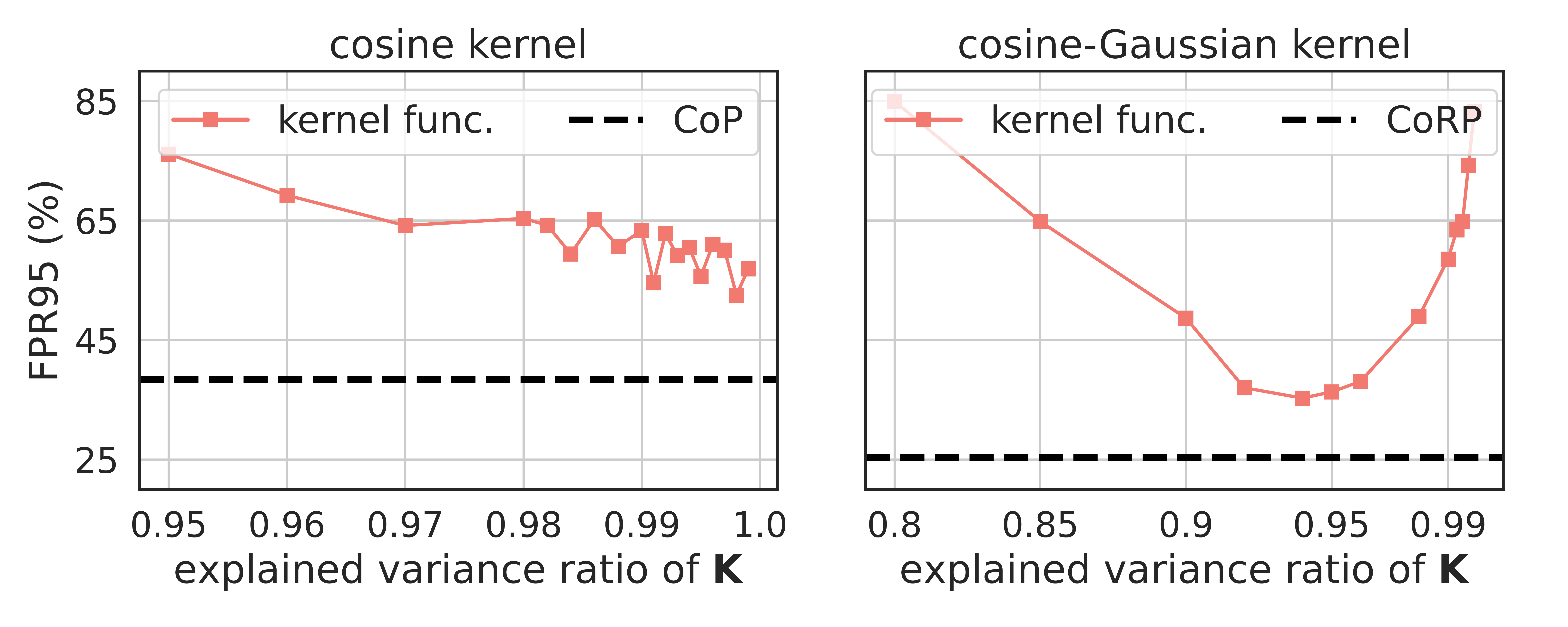
Figure 4: Comparisons on the average detection FPR values between CoP/CoRP and their kernel function implementations in the CIFAR10 benchmark. In experiments, 5,000 images of the CIFAR10 training set and 1,000 images of the CIFAR10 test set and OoD data sets are randomly selected.

This section supplements our covariance-based KPCA with its counterpart that adopts kernel functions. A flexible way to calculate reconstruction errors via kernel functions for OoD detection is presented. Even though, the KPCA with kernel functions is less efficient than CoP/CoRP in two aspects: (i) The time expense of eigendecomposition on the kernel matrix by the former is more expensive than that on the covariance matrix by the latter, since the dimension of the kernel matrix is much larger than that of the covariance matrix. (ii) The former requires an $\mathcal{O}(N_{\rm tr})$ complexity of calculating $\boldsymbol{k}_{\boldsymbol{\hat{z}}}$ in inference, much higher than the $\mathcal{O}(1)$ complexity of the latter.

6 Conclusion

As PCA reconstruction errors fail to distinguish OoD data from InD data on the penultimate features $\boldsymbol{z}$ of DNNs, kernel PCA is introduced for its non-linearity in the manner of employing explicit feature mappings. To find an appropriate feature mapping that can characterize the non-linear patterns in InD and OoD features, we take a kernel perspective on an existing KNN detector [7], and thus propose two explicit feature mappings w.r.t. a cosine kernel and a cosine-Gaussian kernel. The mapped $\Phi(\boldsymbol{z})$-space enables PCA to extract principal components that well separate InD and OoD data, leading to distinguishable reconstruction errors. Extensive empirical results have verified the improved effectiveness and efficiency of the proposed KPCA with new SOTA OoD detection performance. Finally, theoretical discussions and associated experiments are provided to bridge the relationships between our covariance-based KPCA and its kernel function implementation.

One limitation of the KPCA detector is that the two specific kernels are still manually selected with carefully-tuned parameters. It remains a valuable topic in the OoD detection task whether the parameters of kernels could be learned from data according to some optimization objective, i.e., kernel learning. We hope that the proposed two effective kernels verified empirically in our work could benefit the research community as a solid example for future studies.

Supplementary Material for
Kernel PCA for Out-of-Distribution Detection
 

I Details of OoD Detectors Involved in Comparison Experiments

In this section, we elaborate the scoring function $S(\cdot)$ of the OoD detectors included in the comparison experiments of Sec.4.1 and Sec.4.2. Given a well-trained DNN $f:\mathbb{R}^{d}\rightarrow\mathbb{R}^{c}$ with inputs $\boldsymbol{x}\in\mathbb{R}^{d}$, the outputs are $c$-dimension logits $f(\boldsymbol{x})\in\mathbb{R}^{c}$ w.r.t. $c$ classes. The DNN $f$ learns features $\boldsymbol{z}\in\mathbb{R}^{m}$ of $\boldsymbol{x}$ before the last linear layer, i.e., the penultimate features $\boldsymbol{z}$.

MSP [11] employs the softmax function on the output logits and takes the maximum probability as the scoring function. Given a test sample $\boldsymbol{\hat{x}}\in\mathbb{R}^{d}$, its MSP score is

$$S_{\rm MSP}(\boldsymbol{\hat{x}})=\max\left({\rm softmax}(f(\boldsymbol{\hat{x}}))\right).$$ (I.1)

ODIN [12] introduces the temperature scaling and adversarial examples into the MSP score:

$$S_{\rm ODIN}(\boldsymbol{\hat{x}})=\max\left({\rm softmax}(\frac{f(\boldsymbol{\hat{x}}_{\rm a})}{T})\right),$$ (I.2)

where $T$ denotes the temperature and $\boldsymbol{\hat{x}}_{\rm a}$ denotes the perturbed adversarial examples of $\boldsymbol{\hat{x}}$.

Mahalanobis [16] employs the Mahalanobis score to perform OoD detection. The DNN outputs at different layers are modeled as a mixture of multivariate Gaussian distributions and the Mahalanobis distance is calculated. Then, a linear regressor is trained to achieve a weighted Mahalanobis distance at different layers as the final detection score. To train the linear regressor, the training data and the corresponding adversarial examples are adopted as positive and negative samples, respectively.

$$S^{l}_{\rm mahal}(\boldsymbol{\hat{x}}) =\max_{i}\ -(f^{l}(\boldsymbol{\hat{x}})-\boldsymbol{\mu}^{l}_{i})^{T}\boldsymbol{\Sigma}_{l}(f^{l}(\boldsymbol{\hat{x}})-\boldsymbol{\mu}_{i}^{l}),$$ (I.3)

$$S_{\rm mahal}(\boldsymbol{\hat{x}}) =\sum_{l}\alpha_{l}\cdot S^{l}_{\rm mahal}(\boldsymbol{\hat{x}}),$$

where $f^{l}(\boldsymbol{\hat{x}})$ denotes the output features at the $l$-th layer with the associated mean feature vector $\boldsymbol{\mu}^{l}_{i}$ of class-$i$ and the covariance matrix $\boldsymbol{\Sigma}_{l}$, and $\alpha_{l}$ denotes the linear regression coefficients.

Energy [5] adopts an energy function on logits since energy is better aligned with the input probability density:

$$S_{\rm energy}(\boldsymbol{\hat{x}})=\log\sum_{i=1}^{c}\exp(f_{i}(\boldsymbol{\hat{x}})),$$ (I.4)

where $f_{i}(\boldsymbol{\hat{x}})$ denotes the $i$-th element in the $c$-dimension output logits.

GODIN [19] improves ODIN from 2 aspects: decomposing the probabilities and modifying the input pre-processing. On the one hand, a two-branch structure with learnable parameters is imposed after the logits to formulate the decomposed probablities. On the other hand, the magnitude of the adversarial examples is optimized instead of manually tuned in ODIN.

ReAct [14] proposes activation truncation on the penultimate features $\boldsymbol{z}$ of DNNs, as the authors observe that features of OoD data generally hold high unit activations in the penultimate layers. The feature clipping is implemented in a simple way:

$$\boldsymbol{\bar{z}}=\min\left\{\boldsymbol{z},\alpha\right\},$$ (I.5)

where $\alpha$ is a pre-defined constant. The clipped features $\boldsymbol{\bar{z}}$ then pass through the last linear layer and yield modified logits. Other logits-based OoD methods such as Energy could be applied on the modified logits to produce detection scores.

KNN [7] is a simple but time-consuming and memory-inefficient detector since it performs nearest neighbor search on the $\ell_{2}$-normalized penultimate features between the test sample and all the training samples. The negative of the ($k$-th) shortest $\ell_{2}$ distance is set as the score for a new sample $\boldsymbol{\hat{x}}$:

$$S_{\rm knn}(\boldsymbol{\hat{x}})=-\min_{i:1,\cdots,N_{\rm tr}}\left\|\frac{\boldsymbol{\hat{z}}}{\|\boldsymbol{\hat{z}}\|_{2}}-\frac{\boldsymbol{z}_{i}}{\|\boldsymbol{z}_{i}\|_{2}}\right\|_{2},$$ (I.6)

where $\boldsymbol{z}_{i}$ denotes the penultimate features of the $i$-th training sample in the training set of a size $N_{\rm tr}$. The key of this detector is the $\ell_{2}$-normalization on the features.

ViM [26] combines information from both logits and features in a complicated way for OoD detection. Firstly, penultimate features $\boldsymbol{z}$ are projected to the residual space obtained by PCA. Then the norm of projected features gets scaled together with the logits via the softmax function. Finally the scaled feature norm is selected as the detection score.

DICE [25] is a sparsification-based OoD detector by preserving the most important weights in the last linear layer. Denote the weights $\boldsymbol{W}\in\mathbb{R}^{m\times c}$ and the bias $\boldsymbol{b}\in\mathbb{R}^{c}$ in the last linear layer, the forward propagation of DICE is defined as:

$$f_{\rm DICE}(\boldsymbol{\hat{x}})\triangleq\left(\boldsymbol{M}\odot\boldsymbol{W}\right)^{\top}\boldsymbol{\hat{z}}+\boldsymbol{b}.$$ (I.7)

$\odot$ is the element-wise multiplication, and $\boldsymbol{M}\in\mathbb{R}^{m\times c}$ is a masking matrix whose elements are determined by the element-wise multiplication between the $i$-th column $\boldsymbol{w}_{i}\in\mathbb{R}^{m}$ in $\boldsymbol{W}$ and the penultimate features $\boldsymbol{\hat{z}}$: $\boldsymbol{w}_{i}\odot\boldsymbol{\hat{z}}$. Then, similar as ReAct, logits-based detectors could be executed on the modified logits $f_{\rm DICE}(\boldsymbol{\hat{x}})$ to produce detection scores.

BATS [15] proposes to truncate the extreme outputs of Batch Normalization (BN) layers via the estimated mean and standard deviations stored in BN layers, as those extreme features would lead to ambiguity and should be rectified. However, in the released code, the authors actually does not use any information from the BN layers, but instead simply perform clipping on the penultimate features $\boldsymbol{z}$ via the feature mean and standard deviations.

PCA [8] re-formulates the reconstruction errors and empirically shows the inseparativity via the re-formulated errors between InD and OoD data in the primal $\boldsymbol{z}$-space. The authors further propose a regularized reconstruction error and a fusion strategy to boost the OoD detection performance.

We follow the settings in KNN [14] and include CSI [23] and SSD [24] into the comparisons in Sec.4.1. The 2 methods adopt the contrastive losses to train DNNs. In the comparison results of Tab.1 and the following Tab.II.1, the reported detection results w.r.t. CSI and SSD are directly from [7], and are obtained by executing the Mahalanobis detector on learned features of DNNs trained by CSI and SSD. Refer to [14] for more details.

II Supplementary Experiment Results

Table II.1: The detection performance of different methods (ResNet18 trained on CIFAR10) on each OoD data set.

method	OoD data sets
	SVHN		LSUN		iSUN		Textures		Places365		AVERAGE
	FPR$\downarrow$	AUROC$\uparrow$	FPR$\downarrow$	AUROC$\uparrow$	FPR$\downarrow$	AUROC$\uparrow$	FPR$\downarrow$	AUROC$\uparrow$	FPR$\downarrow$	AUROC$\uparrow$	FPR$\downarrow$	AUROC$\uparrow$
Without Supervised Contrastive Learning
MSP	59.66	91.25	45.21	93.80	54.57	92.12	66.45	88.50	62.46	88.64	57.67	90.86
ODIN	20.93	95.55	7.26	98.53	33.17	94.65	56.40	86.21	63.04	86.57	36.16	92.30
Energy	54.41	91.22	10.19	98.05	27.52	95.59	55.23	89.37	42.77	91.02	38.02	93.05
GODIN	15.51	96.60	4.90	99.07	34.03	94.94	46.91	89.69	62.63	87.31	32.80	93.52
Mahalanobis	9.24	97.80	67.73	73.61	6.02	98.63	23.21	92.91	83.50	69.56	37.94	86.50
KNN	24.53	95.96	25.29	95.69	25.55	95.26	27.57	94.71	50.90	89.14	30.77	94.15
CoP (ours)	11.56	97.57	23.24	95.56	53.71	88.74	26.28	93.87	74.11	80.24	37.78	91.20
CoRP (ours)	20.68	96.53	19.19	96.71	21.49	96.26	21.61	96.08	53.73	89.14	27.34	94.95
With Supervised Contrastive Learning
CSI	37.38	94.69	5.88	98.86	10.36	98.01	28.85	94.87	38.31	93.04	24.16	95.89
SSD	1.51	99.68	6.09	98.48	33.60	95.16	12.98	97.70	28.41	94.72	16.52	97.15
KNN	2.42	99.52	1.78	99.48	20.06	96.74	8.09	98.56	23.02	95.36	11.07	97.93
CoP (ours)	0.55	99.85	1.12	99.67	23.91	96.11	4.79	99.06	19.92	95.63	10.06	98.07
CoRP (ours)	0.74	99.82	0.89	99.75	13.08	97.36	4.59	99.03	17.44	95.89	7.35	98.37

II.1 Comparisons with Nearest Neighbor Searching

Tab.II.1 illustrates the comparison results on the CIFAR10 benchmark between our CoP/CoRP and the KNN detector [7]. Similar as the comparisons on the ImageNet-1K benchmark in Tab.1, CoRP outperforms other baselines in both the standard training and the supervised contrastive learning with lower FPR and higher AUROC average values.

Table II.2: Comparisons on the inference time of the KNN detector [7] and our CoP and CoRP. The ImageNet data is of the in-distribution. The experiments are executed on the same machine for a fair comparison. The nearest neighbor searching of KNN is implemented via Faiss [45].

method	time complexity	inference time (ms, per sample)
KNN	$\mathcal{O}(N_{\rm tr})$	$\approx$ 15.59
CoP and CoRP (ours)	$\mathcal{O}(1)$	$\approx$ 0.06

Table II.3: Comparisons on the detection performance between the regularized reconstruction error [8] and the proposed CoP and CoRP fused with other OoD scores (MSP, Energy, ReAct and BATS) on each OoD data set (MobileNet pre-trained on ImageNet-1K).

method	OoD data sets
	iNaturalist		SUN		Places		Textures		AVERAGE
	FPR$\downarrow$	AUROC$\uparrow$	FPR$\downarrow$	AUROC$\uparrow$	FPR$\downarrow$	AUROC$\uparrow$	FPR$\downarrow$	AUROC$\uparrow$	FPR$\downarrow$	AUROC$\uparrow$
MSP	64.29	85.32	77.02	77.10	79.23	76.27	73.51	77.30	73.51	79.00
+ [8]	59.49	86.87	73.75	79.41	76.79	77.94	65.71	83.46	68.93	81.92
+ CoP	57.14	87.62	72.86	79.45	76.17	77.77	60.71	86.42	66.72	82.82
+ CoRP	55.71	88.10	71.48	80.77	75.33	78.90	58.90	87.13	65.36	83.73
Energy	59.50	88.91	62.65	84.50	69.37	81.19	58.05	85.03	62.39	84.91
+ [8]	56.92	89.62	60.07	85.80	69.23	81.72	34.22	91.66	55.11	87.20
+ CoP	51.21	90.79	59.88	85.84	68.62	81.74	23.16	94.55	50.72	88.23
+ CoRP	43.85	91.96	52.17	87.91	63.75	83.59	19.02	95.41	44.70	89.72
ReAct	43.07	92.72	52.47	87.26	59.91	84.07	40.20	90.96	48.91	88.75
+ [8]	35.84	93.66	40.35	90.77	52.38	86.76	18.44	95.39	36.75	91.65
+ CoP	35.84	93.54	48.12	88.97	60.62	84.45	12.62	96.97	39.30	90.98
+ CoRP	31.72	94.27	40.77	90.98	55.69	86.42	10.48	97.49	34.66	92.29
BATS	49.57	91.50	57.81	85.96	64.48	82.83	39.77	91.17	52.91	87.87
+ [8]	50.51	90.86	55.41	87.00	66.43	82.60	23.26	94.70	48.90	88.79
+ CoP	42.68	92.24	55.01	86.89	65.70	82.44	13.78	96.77	44.29	89.58
+ CoRP	36.10	93.37	45.92	89.47	59.82	84.83	11.37	97.24	38.30	91.23
ODIN	58.54	87.51	57.00	85.83	59.87	84.77	52.07	85.04	56.87	85.79
Mahalanobis	62.11	81.00	47.82	83.66	52.09	83.63	92.38	33.06	63.60	71.01
ViM	91.83	77.47	94.34	70.24	93.97	68.26	37.62	92.65	79.44	77.15
DICE	43.28	90.79	38.86	90.41	53.48	85.67	33.14	91.26	42.19	89.53
DICE+ReAct	41.75	89.84	39.07	90.39	54.41	84.03	19.98	95.86	38.80	90.03

Tab.II.2 shows the time-consuming comparison between ours and the KNN detector during inference. The ImageNet-1K benchmark consists of 14,197,122 training images. KNN needs to store and iterate all these features to search the nearest neighbor and costs around 15.59 ms for a new sample, while the iterating process is omitted in our method, resulting in a much higher processing speed, less than 1 ms per sample.

II.2 Comparisons with Regularized Reconstruction Errors

Tab.II.3 shows the comparisons on the MobileNet between our KPCA-based reconstruction errors and the regularized reconstruction errors [8]. Both methods are evaluated under the same fusion strategy with other 4 OoD scores (MSP, Energy, ReAct and BATS). Similar as the results on ResNet50 in Tab.2, the proposed KPCA-based CoP and CoRP outperform [8] in almost all the cases, and CoRP achieves new SOTA OoD detection performance when fused with the ReAct detector. Such results again indicate that the introduced non-linearity of our KPCA could further benefit separating out-distribution samples from in-distribution ones.

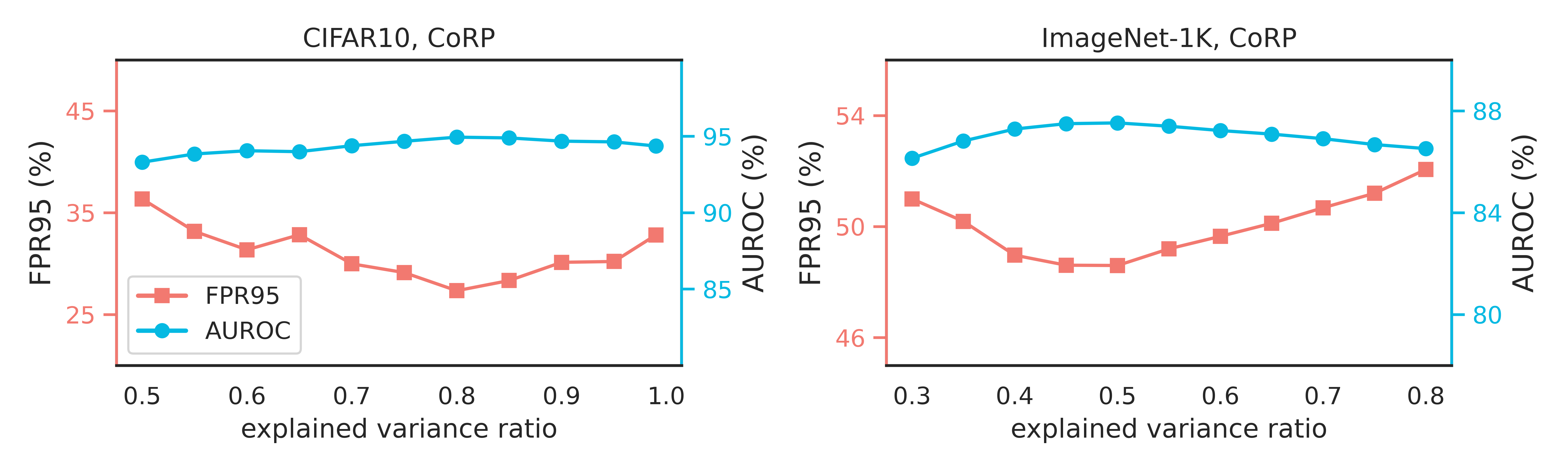
Figure 5: A sensitivity analysis on the explained variance ratio of CoRP. The average detection FPR and AUROC values of OoD data sets in CIFAR10 and ImageNet-1K benchmarks are reported. The Gaussian kernel width $\gamma$ and the dimension $M$ of RFFs are fixed.

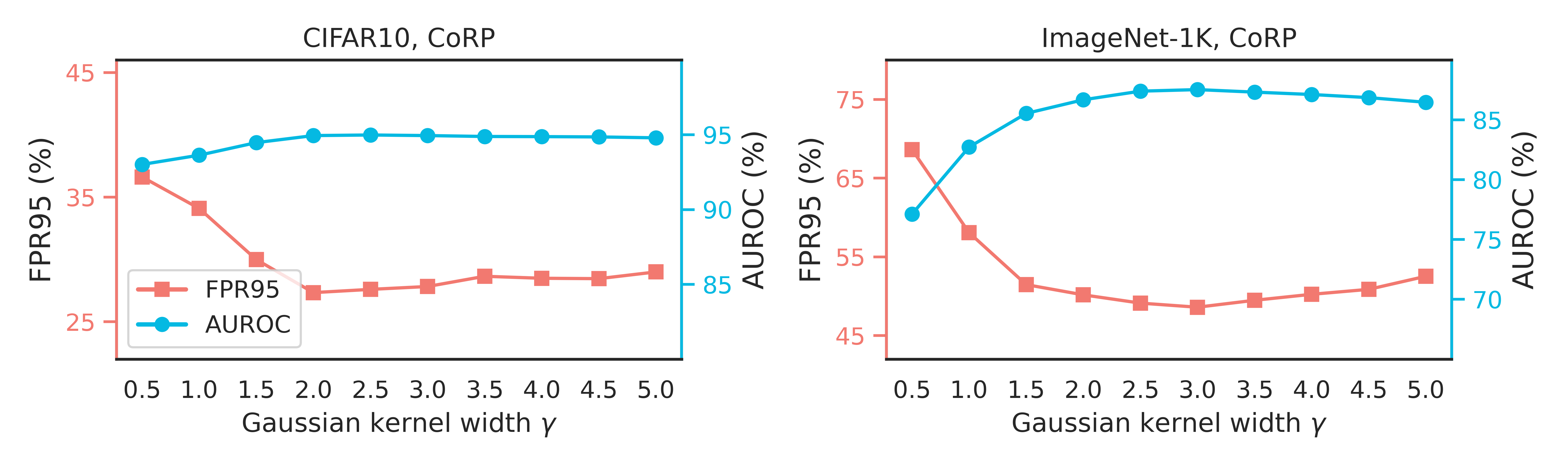
Figure 6: A sensitivity analysis on the Gaussian kernel width $\gamma$ of CoRP. The average detection FPR and AUROC values of OoD data sets in CIFAR10 and ImageNet-1K benchmarks are reported. The explained variance ratio and the dimension $M$ of RFFs are fixed.

II.3 Sensitivity Analysis on CoRP

In this section, a detailed sensitivity analysis on the hyper-parameters of CoRP is provided. Recall the hyper-parameters in CoRP: the Gaussian kernel width $\gamma$, the dimension $M$ of RFFs and the number of columns $q$ of the dimensionality-reduction matrix $\boldsymbol{U}^{\Phi}_{q}$. In the following, we discuss the influence of each hyper-parameter, and report experiment results of the detection performance by varying one hyper-parameter with the other two fixed.

Effect of $q$

As discussed on CoP in Sec.4.3, $q$ determines the fraction of principal components preserved by PCA and is selected based on the explained variance ratio: A high explained variance ratio implies a large value of $q$. Fig.5 shows the detection FPR95 and AUROC values of CoRP w.r.t. different explained variance ratios on CIFAR10 and ImageNet-1K benchmarks. Similar as the case of CoP, an appropriate value of explained variance ratio needs to be carefully selected to achieve the optimal detection performance. Besides, a sufficiently large value of the explained variance ratio is sometimes no longer essential, which might be due to that the 2 concatenated kernels make the useful information for distinguishing out-distribution samples more concentrated in less principal components.

Effect of $\gamma$

The Gaussian kernel width $\gamma$ directly affects the mapped data distribution. For a large $\gamma$, then $k_{\rm gau}(\boldsymbol{z}_{1},\boldsymbol{z}_{2})=e^{-\gamma\left\|\boldsymbol{z}_{1}-\boldsymbol{z}_{2}\right\|_{2}^{2}}\approx 0$ for $\boldsymbol{z}_{1}\neq\boldsymbol{z}_{2}$, which indicates that the mapped features of $\boldsymbol{z}_{1}$ and $\boldsymbol{z}_{2}$ are (nearly) mutually-orthogonal. In this case, a PCA would become meaningless. For a small $\gamma$, then the KPCA-based reconstruction errors will approach the standard PCA-based ones, shown by [46]. Fig.6 illustrates the detection FPR95 and AUROC values of CoRP w.r.t. varied Gaussian kernel width $\gamma$ on CIFAR10 and ImageNet-1K benchmarks. Clearly, neither a too large nor a too small kernel width benefits the detection performance, and a mild value of $\gamma$ should be carefully tuned for different in-distribution data.

Effect of $M$

The dimension $M$ of RFFs determines the approximation ability of RFFs towards the Gaussian kernel. As proved in [27], the larger the $M$, the better the RFFs approximate $k_{\rm gau}$. Fig.7 indicates the detection FPR95 and AUROC values of CoRP w.r.t. multiple values of the RFFs dimension $M$ on CIFAR10 and ImageNet-1K benchmarks. As $M$ increases, the detection performance gets improved since the RFFs better converge to the Gaussian kernel. Considering the computation efficiency of eigendecomposition on the covariance matrix of $\mathbb{R}^{M\times M}$, in the comparison experiments, we adopt $M=4m$ on CIFAR10 with $m=512$ for ResNet18, and $M=2m$ on ImageNet-1K with $m=2048$ for ResNet50 and $m=1280$ for MobileNet.

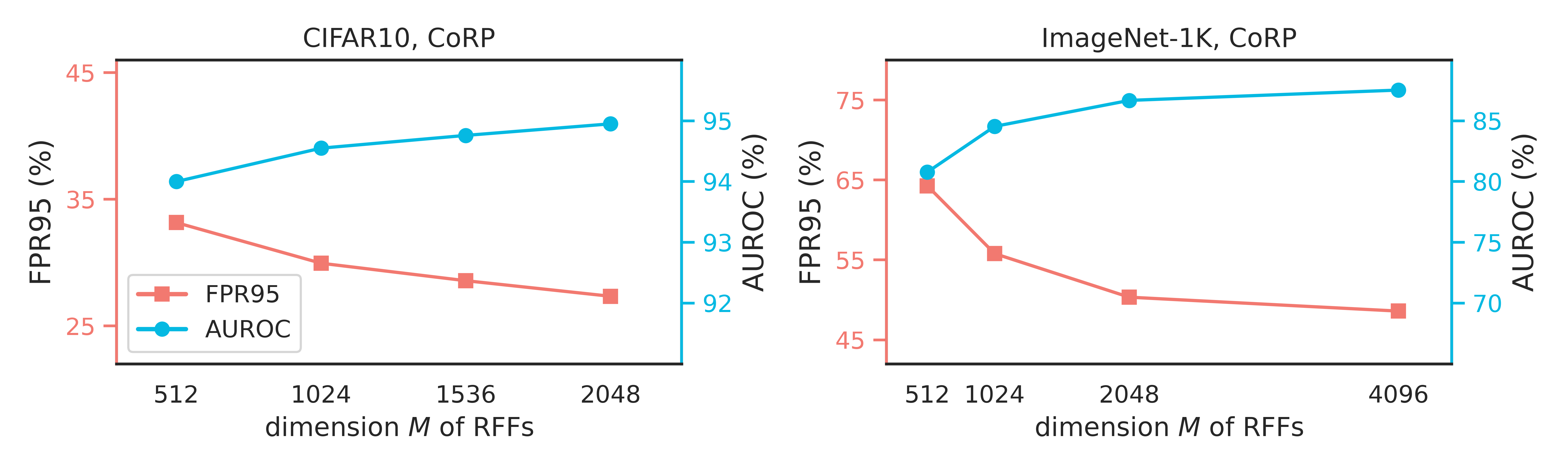
Figure 7: Sensitivity analysis on the dimension $M$ of RFFs of CoRP. The average detection FPR and AUROC values of OoD data sets in CIFAR10 and ImageNet-1K benchmarks are reported. The explained variance ratio and the Gaussian kernel width $\gamma$ are fixed.

III Supplementary Theoretical Results

The proof of Proposition 1 is presented.

Proof.

Recall $\boldsymbol{z}\in\mathbb{R}^{m}$ and suppose $\Phi:\mathbb{R}^{m}\rightarrow\mathbb{R}^{M}$ and $\boldsymbol{U}^{\Phi}\in\mathbb{R}^{M\times M}$ is the eigenvector matrix of the covariance matrix of the training data with $\boldsymbol{U}^{\Phi}=\left[\boldsymbol{U}^{\Phi}_{q},\boldsymbol{U}^{\Phi}_{p}\right]$ and $q+p=M$. For the reconstruction error $e^{\Phi}(\boldsymbol{\hat{z}})$ w.r.t. a new test sample $\boldsymbol{\hat{z}}\in\mathbb{R}^{m}$ in the mapped $\Phi(\boldsymbol{z})$-space, we have:

$$\left(e^{\Phi}(\boldsymbol{\hat{z}})\right)^{2} =\left\|(\Phi(\boldsymbol{\hat{z}})-\boldsymbol{\mu}^{\Phi})-\boldsymbol{U}^{\Phi}_{q}\boldsymbol{U}_{q}^{\Phi\top}(\Phi(\boldsymbol{\hat{z}})-\boldsymbol{\mu}^{\Phi})\right\|_{2}^{2}$$ (III.1)

$$=\left((\Phi(\boldsymbol{\hat{z}})-\boldsymbol{\mu}^{\Phi})-\boldsymbol{U}^{\Phi}_{q}\boldsymbol{U}_{q}^{\Phi\top}(\Phi(\boldsymbol{\hat{z}})-\boldsymbol{\mu}^{\Phi})\right)^{\top}\left((\Phi(\boldsymbol{\hat{z}})-\boldsymbol{\mu}^{\Phi})-\boldsymbol{U}^{\Phi}_{q}\boldsymbol{U}_{q}^{\Phi\top}(\Phi(\boldsymbol{\hat{z}})-\boldsymbol{\mu}^{\Phi})\right)$$

$$=(\Phi(\boldsymbol{\hat{z}})-\boldsymbol{\mu}^{\Phi})^{\top}(\Phi(\boldsymbol{\hat{z}})-\boldsymbol{\mu}^{\Phi})-(\Phi(\boldsymbol{\hat{z}})-\boldsymbol{\mu}^{\Phi})^{\top}\boldsymbol{U}^{\Phi}_{q}\boldsymbol{U}_{q}^{\Phi\top}(\Phi(\boldsymbol{\hat{z}})-\boldsymbol{\mu}^{\Phi})$$

$$=(\Phi(\boldsymbol{\hat{z}})-\boldsymbol{\mu}^{\Phi})^{\top}\left(\boldsymbol{I}-\boldsymbol{U}^{\Phi}_{q}\boldsymbol{U}_{q}^{\Phi\top}\right)(\Phi(\boldsymbol{\hat{z}})-\boldsymbol{\mu}^{\Phi})$$

$$=(\Phi(\boldsymbol{\hat{z}})-\boldsymbol{\mu}^{\Phi})^{\top}\boldsymbol{U}^{\Phi}_{p}\boldsymbol{U}_{p}^{\Phi\top}(\Phi(\boldsymbol{\hat{z}})-\boldsymbol{\mu}^{\Phi})$$

$$=\left\|\boldsymbol{U}_{p}^{\Phi\top}(\Phi(\boldsymbol{\hat{z}})-\boldsymbol{\mu}^{\Phi})\right\|_{2}^{2}.$$

Obviously $e^{\Phi}(\boldsymbol{\hat{z}})=\left\|\boldsymbol{U}_{p}^{\Phi\top}(\Phi(\boldsymbol{\hat{z}})-\boldsymbol{\mu}^{\Phi})\right\|_{2}$ and the proof is finished. ∎

The key in the proof of Proposition 1 is $\boldsymbol{U}_{q}^{\Phi}\boldsymbol{U}_{q}^{\Phi\top}+\boldsymbol{U}_{p}^{\Phi}\boldsymbol{U}_{p}^{\Phi\top}=\boldsymbol{I}$. Since $\boldsymbol{U}^{\Phi}$ is the eigenvector matrix of the covariance matrix, thereby $\boldsymbol{U}^{\Phi}$ is a unitary matrix and satisfies $\boldsymbol{U}^{\Phi}\boldsymbol{U}^{\Phi\top}=\boldsymbol{U}^{\Phi\top}\boldsymbol{U}^{\Phi}=\boldsymbol{I}$, which leads to $\boldsymbol{U}_{q}^{\Phi}\boldsymbol{U}_{q}^{\Phi\top}+\boldsymbol{U}_{p}^{\Phi}\boldsymbol{U}_{p}^{\Phi\top}=\boldsymbol{I}$.

References

- Ho et al. [2020] Jonathan Ho, Ajay Jain, and Pieter Abbeel. Denoising diffusion probabilistic models. Advances in neural information processing systems, 33:6840–6851, 2020.
- Ouyang et al. [2022] Long Ouyang, Jeffrey Wu, Xu Jiang, Diogo Almeida, Carroll Wainwright, Pamela Mishkin, Chong Zhang, Sandhini Agarwal, Katarina Slama, Alex Ray, et al. Training language models to follow instructions with human feedback. Advances in Neural Information Processing Systems, 35:27730–27744, 2022.
- Barrett et al. [2023] Clark Barrett, Brad Boyd, Ellie Burzstein, Nicholas Carlini, Brad Chen, Jihye Choi, Amrita Roy Chowdhury, Mihai Christodorescu, Anupam Datta, Soheil Feizi, et al. Identifying and mitigating the security risks of generative ai. arXiv preprint arXiv:2308.14840, 2023.
- Yang et al. [2021] Jingkang Yang, Kaiyang Zhou, Yixuan Li, and Ziwei Liu. Generalized out-of-distribution detection: A survey. arXiv preprint arXiv:2110.11334, 2021.
- Liu et al. [2020] Weitang Liu, Xiaoyun Wang, John Owens, and Yixuan Li. Energy-based out-of-distribution detection. Advances in neural information processing systems, 33:21464–21475, 2020.
- Huang et al. [2021] Rui Huang, Andrew Geng, and Yixuan Li. On the importance of gradients for detecting distributional shifts in the wild. Advances in Neural Information Processing Systems, 34:677–689, 2021.
- Sun et al. [2022] Yiyou Sun, Yifei Ming, Xiaojin Zhu, and Yixuan Li. Out-of-distribution detection with deep nearest neighbors. In International Conference on Machine Learning, pages 20827–20840. PMLR, 2022.
- Guan et al. [2023] Xiaoyuan Guan, Zhouwu Liu, Wei-Shi Zheng, Yuren Zhou, and Ruixuan Wang. Revisit pca-based technique for out-of-distribution detection. In Proceedings of the IEEE/CVF International Conference on Computer Vision, pages 19431–19439, 2023.
- Van der Maaten and Hinton [2008] Laurens Van der Maaten and Geoffrey Hinton. Visualizing data using t-sne. Journal of machine learning research, 9(11), 2008.
- Schölkopf et al. [1997] Bernhard Schölkopf, Alexander Smola, and Klaus-Robert Müller. Kernel principal component analysis. In International conference on artificial neural networks, pages 583–588. Springer, 1997.
- Hendrycks and Gimpel [2016] Dan Hendrycks and Kevin Gimpel. A baseline for detecting misclassified and out-of-distribution examples in neural networks. In International Conference on Learning Representations, 2016.
- Liang et al. [2018] Shiyu Liang, Yixuan Li, and R Srikant. Enhancing the reliability of out-of-distribution image detection in neural networks. In International Conference on Learning Representations, 2018.
- Wu et al. [2023] Yingwen Wu, Tao Li, Xinwen Cheng, Jie Yang, and Xiaolin Huang. Low-dimensional gradient helps out-of-distribution detection. arXiv preprint arXiv:2310.17163, 2023.
- Sun et al. [2021] Yiyou Sun, Chuan Guo, and Yixuan Li. React: Out-of-distribution detection with rectified activations. Advances in Neural Information Processing Systems, 34:144–157, 2021.
- Zhu et al. [2022] Yao Zhu, YueFeng Chen, Chuanlong Xie, Xiaodan Li, Rong Zhang, Hui Xue, Xiang Tian, Yaowu Chen, et al. Boosting out-of-distribution detection with typical features. Advances in Neural Information Processing Systems, 35:20758–20769, 2022.
- Lee et al. [2018] Kimin Lee, Kibok Lee, Honglak Lee, and Jinwoo Shin. A simple unified framework for detecting out-of-distribution samples and adversarial attacks. Advances in neural information processing systems, 31, 2018.
- Yu et al. [2023] Yeonguk Yu, Sungho Shin, Seongju Lee, Changhyun Jun, and Kyoobin Lee. Block selection method for using feature norm in out-of-distribution detection. In Proceedings of the IEEE/CVF Conference on Computer Vision and Pattern Recognition, pages 15701–15711, 2023.
- Song et al. [2022] Yue Song, Nicu Sebe, and Wei Wang. Rankfeat: Rank-1 feature removal for out-of-distribution detection. Advances in Neural Information Processing Systems, 35:17885–17898, 2022.
- Hsu et al. [2020] Yen-Chang Hsu, Yilin Shen, Hongxia Jin, and Zsolt Kira. Generalized odin: Detecting out-of-distribution image without learning from out-of-distribution data. In Proceedings of the IEEE/CVF Conference on Computer Vision and Pattern Recognition, pages 10951–10960, 2020.
- Fang et al. [2023a] Kun Fang, Qinghua Tao, Xiaolin Huang, and Jie Yang. Revisiting deep ensemble for out-of-distribution detection: A loss landscape perspective. arXiv preprint arXiv:2310.14227, 2023a.
- Ye et al. [2021] Haotian Ye, Chuanlong Xie, Tianle Cai, Ruichen Li, Zhenguo Li, and Liwei Wang. Towards a theoretical framework of out-of-distribution generalization. Advances in Neural Information Processing Systems, 34:23519–23531, 2021.
- Fang et al. [2022] Zhen Fang, Yixuan Li, Jie Lu, Jiahua Dong, Bo Han, and Feng Liu. Is out-of-distribution detection learnable? Advances in Neural Information Processing Systems, 35:37199–37213, 2022.
- Tack et al. [2020] Jihoon Tack, Sangwoo Mo, Jongheon Jeong, and Jinwoo Shin. Csi: Novelty detection via contrastive learning on distributionally shifted instances. Advances in neural information processing systems, 33:11839–11852, 2020.
- Sehwag et al. [2020] Vikash Sehwag, Mung Chiang, and Prateek Mittal. Ssd: A unified framework for self-supervised outlier detection. In International Conference on Learning Representations, 2020.
- Sun and Li [2022] Yiyou Sun and Yixuan Li. Dice: Leveraging sparsification for out-of-distribution detection. In European Conference on Computer Vision, pages 691–708. Springer, 2022.
- Wang et al. [2022] Haoqi Wang, Zhizhong Li, Litong Feng, and Wayne Zhang. Vim: Out-of-distribution with virtual-logit matching. In Proceedings of the IEEE/CVF Conference on Computer Vision and Pattern Recognition, pages 4921–4930, 2022.
- Rahimi and Recht [2007] Ali Rahimi and Benjamin Recht. Random features for large-scale kernel machines. Advances in neural information processing systems, 20, 2007.
- Rudin [1962] Walter Rudin. Fourier analysis on groups, volume 121967. Wiley Online Library, 1962.
- Fang et al. [2023b] Kun Fang, Fanghui Liu, Xiaolin Huang, and Jie Yang. End-to-end kernel learning via generative random fourier features. Pattern Recognition, 134:109057, 2023b.
- Belkin et al. [2019] Mikhail Belkin, Daniel Hsu, Siyuan Ma, and Soumik Mandal. Reconciling modern machine-learning practice and the classical bias–variance trade-off. Proceedings of the National Academy of Sciences, 116(32):15849–15854, 2019.
- Krizhevsky [2009] A Krizhevsky. Learning multiple layers of features from tiny images. Master’s thesis, University of Toronto, 2009.
- Deng et al. [2009] Jia Deng, Wei Dong, Richard Socher, Li-Jia Li, Kai Li, and Li Fei-Fei. Imagenet: A large-scale hierarchical image database. In IEEE Conference on Computer Vision and Pattern Recognition, pages 248–255, 2009.
- Netzer et al. [2011] Yuval Netzer, Tao Wang, Adam Coates, Alessandro Bissacco, Bo Wu, and Andrew Y Ng. Reading digits in natural images with unsupervised feature learning. In Proceedings of the NIPS Workshop on Deep Learning and Unsupervised Feature Learning, 2011.
- Yu et al. [2015] Fisher Yu, Ari Seff, Yinda Zhang, Shuran Song, Thomas Funkhouser, and Jianxiong Xiao. Lsun: Construction of a large-scale image dataset using deep learning with humans in the loop. arXiv preprint arXiv:1506.03365, 2015.
- Xu et al. [2015] Pingmei Xu, Krista A Ehinger, Yinda Zhang, Adam Finkelstein, Sanjeev R Kulkarni, and Jianxiong Xiao. Turkergaze: Crowdsourcing saliency with webcam based eye tracking. arXiv preprint arXiv:1504.06755, 2015.
- Cimpoi et al. [2014] Mircea Cimpoi, Subhransu Maji, Iasonas Kokkinos, Sammy Mohamed, and Andrea Vedaldi. Describing textures in the wild. In Proceedings of the IEEE conference on computer vision and pattern recognition, pages 3606–3613, 2014.
- Zhou et al. [2017] Bolei Zhou, Agata Lapedriza, Aditya Khosla, Aude Oliva, and Antonio Torralba. Places: A 10 million image database for scene recognition. IEEE transactions on pattern analysis and machine intelligence, 40(6):1452–1464, 2017.
- Van Horn et al. [2018] Grant Van Horn, Oisin Mac Aodha, Yang Song, Yin Cui, Chen Sun, Alex Shepard, Hartwig Adam, Pietro Perona, and Serge Belongie. The inaturalist species classification and detection dataset. In Proceedings of the IEEE conference on computer vision and pattern recognition, pages 8769–8778, 2018.
- Xiao et al. [2010] Jianxiong Xiao, James Hays, Krista A Ehinger, Aude Oliva, and Antonio Torralba. Sun database: Large-scale scene recognition from abbey to zoo. In 2010 IEEE computer society conference on computer vision and pattern recognition, pages 3485–3492. IEEE, 2010.
- Khosla et al. [2020] Prannay Khosla, Piotr Teterwak, Chen Wang, Aaron Sarna, Yonglong Tian, Phillip Isola, Aaron Maschinot, Ce Liu, and Dilip Krishnan. Supervised contrastive learning. Advances in neural information processing systems, 33:18661–18673, 2020.
- He et al. [2016] Kaiming He, Xiangyu Zhang, Shaoqing Ren, and Jian Sun. Deep residual learning for image recognition. In IEEE Conference on Computer Vision and Pattern Recognition, pages 770–778, 2016.
- Sandler et al. [2018] Mark Sandler, Andrew Howard, Menglong Zhu, Andrey Zhmoginov, and Liang-Chieh Chen. Mobilenetv2: Inverted residuals and linear bottlenecks. In Proceedings of the IEEE conference on computer vision and pattern recognition, pages 4510–4520, 2018.
- Paszke et al. [2019] Adam Paszke, Sam Gross, Francisco Massa, Adam Lerer, James Bradbury, Gregory Chanan, Trevor Killeen, Zeming Lin, Natalia Gimelshein, Luca Antiga, et al. Pytorch: An imperative style, high-performance deep learning library. Advances in neural information processing systems, 32, 2019.
- Kwok and Tsang [2004] JT-Y Kwok and IW-H Tsang. The pre-image problem in kernel methods. IEEE transactions on neural networks, 15(6):1517–1525, 2004.
- Johnson et al. [2019] Jeff Johnson, Matthijs Douze, and Hervé Jégou. Billion-scale similarity search with gpus. IEEE Transactions on Big Data, 7(3):535–547, 2019.
- Hoffmann [2007] Heiko Hoffmann. Kernel pca for novelty detection. Pattern recognition, 40(3):863–874, 2007.