Encoding quantum optical states with classical wireless microwave constellation

Abstract

This paper explores the underlying physics behind seamless transduction of digital information encoded in the classical microwave domain to the quantum optical domain. We comprehensively model the quantum mechanical interaction mediating the transduction in a seamless wireless-to-optical converter. We highlight that the quantum mechanical interaction can be enhanced by suitably choosing the physical width and the inter-modulating element spacing in the converter. This study also highlights the encoding of quantum optical phase-space with classical microwave constellation. Furthermore, the challenge of inter-symbol overlap in the encoded quantum optical phase-space due to quantum shot noise is addressed. The reported findings provide a foundational framework for bridging classical microwave and quantum optical communication links in the future.

I Introduction

Microwave and optical photons play crucial roles in quantum information processing and networking Sahu et al. (2022). Over the years, several technological platforms have emerged as promising candidates for quantum information processing in the microwave and optical frequency domains Blümel et al. (2021); Ringbauer et al. (2022); Covey et al. (2023); Park et al. (2022); Hendrickx et al. (2020); Blumoff et al. (2022); Krantz et al. (2019); Liu et al. (2020); Wu et al. (2020a). In order to deploy feasible distributed quantum networks in the future, numerous microwave quantum processing units operating at cryogenic environments must be seamlessly interlinked by low-loss fibers carrying optical photons at room temperature Han et al. (2021). The efficiency and reliability of such networks shall heavily depend on coherent microwave-to-optical photon transduction Mirhosseini et al. (2020). Several technological platforms are being explored for enabling coherent microwave-to-optical photon transduction, including electro-optical conversion Fu et al. (2021); Soltani et al. (2017); Rueda et al. (2016), magnon-mediated conversion Xie et al. (2023); Zhu et al. (2020); Zhang et al. (2016), atom-assisted conversion Kumar et al. (2023); Liao et al. (2023); Adwaith et al. (2019), and optomechanical conversion Kim et al. (2023); Zhong et al. (2022); Wu et al. (2020b). Among these, electro-optic conversion stands out as one of the most promising platforms owing to the absence of intermediary stages and good conversion efficiency, thereby enabling seamless microwave-to-optical photon transduction Xu et al. (2021).

Seamless microwave-to-optical transduction additionally paves the way for bridging classical and quantum communication links in the future. Particularly, integrating classical wireless microwave and quantum optical links shall lay the foundation for several advanced quantum-enhanced applications in the future. Numerous studies delved into various interesting aspects of classical-microwave to quantum-optical transduction mediated by Pockel’s electro-optic effect. A comprehensive quantum optical description of an electro-optic phase-modulator was reported Capmany and Fernández-Pousa (2010). The quantum optical modeling of electro-optic phase-modulation considering the effects of perturbative dispersion was detailed in Horoshko et al. (2018). The impact of classical microwave phase-noise in electro-optic phase-modulation of a quantum optical mode was reported in Pratap and Ramachandran (2020). Recent research also reported the quantum mechanical description of a dual-drive Mach-Zehnder modulator for coherent quantum optical communication links Pratap and Ramachandran (2023). Furthermore, the experimental characterization of quantum optical sideband generation in electro-optic phase-modulation was carried out through a two-photon interference experiment Imany et al. (2018).

At this juncture, it is important to reiterate that most modern wireless communication systems transmit information by encapsulating digital data in high-frequency microwave carriers Haykin (1988). Therefore, to envision seamless integration of classical microwave wireless and quantum optical links, it is important to first investigate how digital data encapsulated in classical microwave carriers can be mapped to the quantum optical domain. Some of our recent works revolve around seamless microwave-to-optical digital information mapping for classical wireless-over-optical links. We modeled wireless-to-optical digital phase-mapping using novel bi-layered electro-optic modulation scheme in Ghosh and Pendharker (2021). Recently, we reported our investigations on novel electro-optic beamforming in seamless wireless-to-optical digital constellation mapping N. Ghosh and S. Pendharker (2023). We further extended our investigations to proposing a novel architecture enabling photonic-based digital microwave constellation detection, forming the basis for bridging classical digital microwave and optical communication links Ghosh and Pendharker (2023). However, the aspect of digital information mapping from the classical-microwave to the quantum-optical domain remains unexplored so far.

This paper investigates seamless transduction of digital information from the classical microwave domain to the quantum optical domain. This paper is organized as follows. In section II, we discuss a versatile framework based on Schrodinger’s picture for characterizing and understanding classical-microwave to the quantum-optical digital information transduction. We first derive the Hamiltonian describing the electro-optic interaction between a quantum optical mode and a digitally modulated classical microwave carrier received by a Wireless-to-Optical (W-O) converter. Using Schrodinger’s picture, we model the converter as an equivalent quantum mechanical network for understanding and visualizing the evolution of the modulated quantum optical mode. We highlight that the electro-optic interaction-strength can be maximized by suitably choosing the modulating element width present in the converter. In section III, we show that the electro-optic interaction strength can further be enhanced by appropriately choosing the inter-element spacing in a modulating-element array-based W-O converter, supported by physical reasoning. In section IV, we use the derived interaction model to demonstrate seamless encoding of quantum optical phase-space with classical microwave constellation. We also derive an equivalent unitary operator to model the discussed encoding scheme. Mitigation of inter-symbol overlap due to quantum optical shot noise in the encoded optical phase-space is also discussed. The reported novel contributions in this paper lay the theoretical groundwork for seamless bridging of digital classical microwave and quantum optical links in the future.

II Digitally encoded classical microwave to quantum optical transduction

II.1 Electro-optic interaction Hamiltonian

Figure 1 illustrates a seamless electro-optic phase-modulator based W-O converter. The converter comprises of a Lithium Niobate (LiNbO₃) optical waveguide channelized through a centrally slotted patch antenna working as the modulating element. The waveguide dimension was chosen as 608nm x 164nm to enable single-mode optical propagation of wavelength 1555$nm$. The effective refractive index $n_{op}$ of the optical waveguide was computed to be 1.734 using effective-index method N. Ghosh and S. Pendharker (2023). We consider an $x$-polarized quantum optical mode of frequency $\omega_{op}$ propagating along the $z$-direction to be launched at the input end of the waveguide. The electric-field operator $\hat{E}_{op}(t)$ of the quantum optical mode is Gerry and Knight (2023),

$$\hat{E}_{op}(t)=j\sqrt{\frac{\hbar\omega_{op}}{2\epsilon_{o}\epsilon_{op}V}}\ \bigg{(}\hat{a}\ e^{-j(\omega_{op}t-k_{op}z)}-\hat{a}^{\dagger}\ e^{j(\omega_{op}t-k_{op}z)}\bigg{)}$$ (1)

where $k_{op}$ is the phase-constant of the quantum optical mode, $\epsilon_{o}$ is the permittivity of vacuum, and $\epsilon_{op}$ is the effective relative permittivity of the optical waveguide. Also, $\hat{a}^{\dagger}$ and $\hat{a}$ are the creation and annihilation operators associated with the quantum optical mode, respectively. In the absence of classical microwave reception, the total Hamiltonian of the quantum optical mode traveling through the converter is equal to the free Hamiltonian $\hat{H}_{o}$ of a quantum harmonic oscillator Bransden (2000),

$$\hat{H}_{o}=\int_{V}\frac{1}{2}\ \epsilon_{o}\ \epsilon_{op}\ \hat{E}_{op}{(t)}.\hat{E}_{op}{(t)}\ dV=\hbar\omega_{op}\big{(}\hat{a}^{\dagger}\hat{a}+\frac{1}{2}\big{)}$$ (2)

We next consider an $x$-polarized classical wireless microwave E-field $E_{w}(t)$ to be received by the converter,

$$E_{w}(t)=|E_{w}|\ \sin{(\omega_{w}t+b_{i})}$$ (3)

.

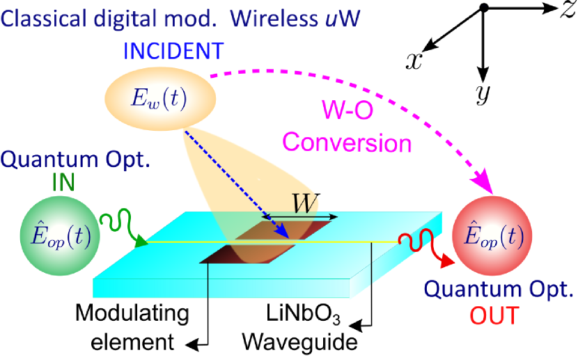
Figure 1: Digitally modulated classical wireless microwave to quantum optical transduction in a seamless W-O converter.

where $|E_{w}|$ and $\omega_{w}$ is the field-strength and frequency of $E_{w}(t)$, respectively. We consider $E_{w}(t)$ to be digital phase-shift-keyed (PSK) modulated Haykin (1988), where $b_{i}$ is the phase associated with the $i^{th}$ digital symbol encapsulated in $E_{w}(t)$. On receiving $E_{w}(t)$, an $x$-polarized E-field of enhanced field-strength gets induced in the centrally slotted modulating element Ghosh and Pendharker (2021). Consequently, Pockel’s electro-optic effect perturbs $\epsilon_{op}$ of the LiNbO₃ optical waveguide section channelized through the modulating element. Considering the optic-axis of the LiNbO₃ waveguide to be oriented along the $x$-axis, the Pockel’s effect induced perturbation can be expressed as follows,

$$\epsilon^{\prime}_{op}(t)=\epsilon_{op}+\delta\epsilon_{op}(t)=\epsilon_{op}-\epsilon_{op}^{2}r_{33}\gamma E_{w}(t)$$ (4)

where $\delta\epsilon_{op}(t)$=$-\epsilon_{op}^{2}r_{33}\gamma E_{w}(t)$ is the perturbed relative permittivity of the wavguide, $r_{33}$ is the Pockel’s electro-optic coefficient of LiNbO₃, and $\gamma$ is the slot field-strength enhancement factor. The total Hamiltonian $\hat{H}(t)$ of the quantum optical mode in this case becomes (see Appendix-A),

$$\begin{split}\hat{H}(t)&=\int_{V}\frac{1}{2}\ \epsilon_{o}\ \epsilon^{\prime}_{op}(t)\ \hat{E}_{op}{(t)}.\hat{E}_{op}{(t)}\ dV\\ &=\hbar\omega_{op}\hat{a}^{\dagger}\hat{a}-\frac{\epsilon_{op}r_{33}}{2}\gamma E_{w}(t)\ \hbar\omega_{op}\hat{a}^{\dagger}\hat{a}\\ &=\hat{H_{o}}+\hat{H}_{I}(t)\end{split}$$ (5)

where $\hat{H}_{I}(t)$ is the time-dependent Hamiltonian associated with the electro-optic interaction between the quantum optical mode and the received classical microwave E-field. The expression of the interaction Hamiltonian $\hat{H}_{I}(t)$ is,

$$\hat{H}_{I}(t)=-\frac{\epsilon_{op}r_{33}}{2}\gamma E_{w}(t)\ \hbar\omega_{op}\hat{a}^{\dagger}\hat{a}$$ (6)

In the upcoming subsection, we derive the evolution of the quantum optical mode electro-optically interacting with the received classical microwave E-field.

II.2 Evolution of modulated quantum optical state

The time evolution of the quantum optical state $\ket{\psi}$ due to electro-optic interaction in the modulating element is governed by the time-dependent Schrodinger’s equation as follows,

$$j\hbar\frac{d\ket{\psi(t)}}{dt}=\hat{H}(t)\ket{\psi(t)}$$ (7)

The general solution of time-dependent Schrodinger’s equation is of the following form,

$$\ket{\psi(t)}=\sum_{k=0}^{\infty}\ket{\psi_{k}(t)}=\sum_{k=0}^{\infty}C_{k}(t)\ket{k}$$ (8)

where $C_{k}(t)$ is the time-evolving probability amplitude of the $k^{th}$ photon number-state $\ket{k}$ of the quantum optical state $\ket{\psi}$. By substituting the expression of $\ket{\psi(t)}$ from Eq. (8) in Eq. (7), we get the following differential equation,

$$j\hbar\sum_{k=0}^{\infty}\frac{dC_{k}(t)}{dt}\ket{k}=\sum_{k=0}^{\infty}\hat{H}(t)C_{k}(t)\ket{k}$$ (9)

For the sake of simplicity, we consider the quantum optical state propagating through the modulating element to be a single photon state i.e. $\ket{\psi(t)}$=$\ket{\psi_{1}(t)}$. By substituting the expression of $\hat{H}(t)$ from Eq. (5) to Eq. (9), we get the following differential equation,

$$j\hbar\frac{dC_{1}(t)}{dt}=\hbar\omega_{op}\bigg{(}1-\frac{\epsilon_{op}r_{33}}{2}\ \gamma E_{w}(t)\bigg{)}C_{1}(t)$$ (10)

where $C_{1}(t)$ is the time-evolving probability amplitude of the single optical photon state $\ket{\psi_{1}}$.

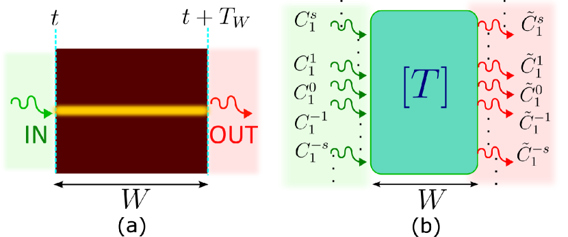
Figure 2: (a) Modulating element of width $W$ in the W-O converter. (b) Equivalent quantum mechanical network model of the modulating element.

The time-evolving probability amplitude $C_{1}(t)$ of the single optical photon state $\ket{\psi_{1}(t)}$ can be derived by integrating Eq. (10) in the time window during which it interacts with the received classical microwave E-field in the modulating element. We consider the optical photon state to enter the modulating element of width $W$ at the time instant $t$, and exit at the time instant $(t+T_{W})$, as depicted in Fig. 2(a). Here $T_{W}$=$(W\sqrt{\epsilon_{op}}/c)$ is the time taken by the optical photon to travel the distance $W$ in the waveguide. The probability amplitude $C_{1}(t)$ of the optical photon state at the output of the modulating element can therefore be derived to be (see Appendix-B),

$$\tilde{C}_{1}=C_{1}\ e^{-j(\omega_{op}t+k_{op}W+\theta_{i}(t))}$$ (11)

where $\tilde{C}_{1}$ is the probability amplitude of the optical photon at the output of the modulating element, and $C_{1}$ is its initial probability amplitude. Also, $\theta_{i}(t)$ is the phase encoded in the complex probability amplitude of the modulated optical photon. The modulated quantum optical phase $\theta_{i}(t)$ is related to the digital phase $b_{i}$ of the received classical M-PSK microwave E-field as follows,

$$\theta_{i}(t)=\delta\theta\sin{(\omega_{w}t+\phi+b_{i})}$$ (12)

where $\delta\theta$ represents the electro-optic modulation-depth, which can be expressed as follows,

$$\delta\theta=-\frac{\omega_{op}\epsilon_{op}r_{33}}{\omega_{w}}\ \gamma|E_{w}|\ \sin{\bigg{(}\frac{\omega_{w}\sqrt{\epsilon_{op}}W}{2c}\bigg{)}}$$ (13)

Also the offset phase term $\phi$ in Eq. (12) can be expressed as,

$$\phi=\frac{\omega_{w}\sqrt{\epsilon_{op}}W}{2c}$$ (14)

Substituting the expression of $\theta_{i}(t)$ from Eq. (12) in Eq. (11), and expanding the resultant equation using Jacobi-Anger expansion, we get the following expression,

$$\tilde{C_{1}}=C_{1}e^{-j(\omega_{op}t+k_{op}W)}\sum^{s=-\infty}_{s=\infty}j^{s}J_{s}(\delta\theta)\ e^{-js({\omega_{w}}t+\phi+b_{i})}$$ (15)

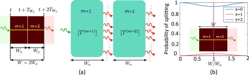
Figure 3: (a) Equivalent quantum mechanical network model of a modulating element of width $W$=$2W_{o}$. (b) Variation of probability amplitude splitting of a modulated optical photon with a variation in the modulating element width, considering a classical microwave reception of field-strength $|E_{w}|$=50V/m.

Equation (15) indicates that the probability amplitude of the modulated optical photon splits into various sidebands evolving at frequencies $(\omega_{op}\pm s\omega_{w})$ (where $s$=0,1,2,3,…). Therefore, the modulating element can be ideally modeled as an infinite-port quantum mechanical network, as depicted in Fig 2(b). In the equivalent network, each port denoted by ${C^{s}_{1}}$ represents the $s^{th}$ sideband probability amplitude of the unmodulated optical photon at the input of the network. Similarly, each port denoted by $\tilde{C^{s}_{1}}$ represents the $s^{th}$ sideband probability amplitude of the modulated optical photon at the output of the network. The output probability amplitude vector $[\tilde{C^{s}_{1}}]$ can be related to the input probability amplitude vector $[{C^{s}_{1}}]$ by an equivalent infinite-dimensional transmission matrix $[T]$, expressed below (see Appendix-B),

$$[T]=e^{-jk_{op}W}\begin{bmatrix}\textbf{.}&\textbf{.}&\textbf{.}&\textbf{.}&\textbf{.}&\textbf{.}&\textbf{.}\\ \textbf{.}&\textbf{.}&\textbf{.}&\textbf{.}&\textbf{.}&\textbf{.}&\textbf{.}\\ \textbf{.}&\textbf{.}&J_{0}(\delta\theta)&j^{-1}J_{-1}(\delta\theta)e^{j(\omega_{w}t+\phi+b_{i})}&j^{-2}J_{-2}(\delta\theta)e^{j2(\omega_{w}t+\phi+b_{i})}&\textbf{.}&\textbf{.}\\ \textbf{.}&\textbf{.}&jJ_{1}(\delta\theta)e^{-j(\omega_{w}t+\phi+b_{i})}&J_{0}(\delta\theta)&j^{-1}J_{-1}(\delta\theta)e^{j(\omega_{w}t+\phi+b_{i})}&\textbf{.}&\textbf{.}\\ \textbf{.}&\textbf{.}&j^{2}J_{2}(\delta\theta)e^{-j2(\omega_{w}t+\phi+b_{i})}&j^{1}J_{1}(\delta\theta)e^{-j(\omega_{w}t+\phi+b_{i})}&J_{0}(\delta\theta)&\textbf{.}&\textbf{.}\\ \textbf{.}&\textbf{.}&\textbf{.}&\textbf{.}&\textbf{.}&\textbf{.}&\textbf{.}\\ \textbf{.}&\textbf{.}&\textbf{.}&\textbf{.}&\textbf{.}&\textbf{.}&\textbf{.}\end{bmatrix}$$ (16)

Therefore, at the output of the modulating element, the optical photon can remain at the center frequency $\omega_{op}$ with probability $J^{2}_{0}(\delta\theta)$, or shift to the frequency $(\omega_{op}\pm s\omega_{w})$ with probability $J^{2}_{\pm s}(\delta\theta)$. The extent of probability amplitude splitting is an indicator of the electro-optic modulation-depth. In the upcoming subsection, we show that the probability amplitude splitting can be maximized by suitably choosing the physical width $W$ of the modulating element in the W-O converter.

II.3 Maximizing probability amplitude splitting in a modulating element

From Eq. (13), it can be found that the electro-optic modulation-depth $\delta\theta$ can be maximized if the modulating element width is chosen as $W$=$W_{o}$=$(\pi c/2\omega_{w}\sqrt{\epsilon_{op}})$. The maximized electro-optic modulation-depth $\delta\theta$=$\delta\theta_{o}$ in that case becomes equal to,

$$\delta\theta_{o}=-\frac{\omega_{op}\epsilon_{op}r_{33}}{\omega_{w}}\ \gamma|E_{w}|$$ (17)

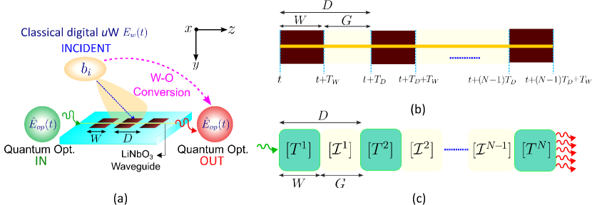
Figure 4: (a) Schematic of a W-O converter comprising of multiple cascaded modulating elements. (b) Schematic of the N-element modulating array of optimum width $W_{o}$ cascaded at periodicity $D$. (c) Quantum mechanical network modeling of an $N$-element modulating array.

Additionally, it can also be found that if the width is chosen as twice the optimum width i.e. $W$=$2W_{o}$=$(\pi c/\omega_{w}\sqrt{\epsilon_{op}})$, the electro-optic modulation-depth $\delta\theta$ becomes zero, irrespective of the received classical microwave E-field. This can be explained using the previously derived quantum mechanical network model. To do this, we first consider the physical width $W$ of the modulating element to be $W$=$2W_{o}$. We then divide the entire modulating element into two individual sections of width $W_{o}$ cascaded to each other, as shown in Fig. 3(a). We then model each section as equivalent infinite-port quantum mechanical networks $m$=$1$ and $m$=$2$ having transmission matrices $[T^{(m=1)}]$ and $[T^{(m=2)}]$, respectively. Since the two networks are cascaded to each other, the overall transmission matrix $[T]$ of the entire modulating element is the product of $[T^{(m=1)}]$ and $[T^{(m=2)}]$ i.e. $[T]$=$[T^{(m=2)}][T^{(m=1)}]$. In Appendix-C, it has been shown that $[T^{(m=2)}]=e^{-j2k_{op}W_{o}}[T^{(m=1)}]^{-1}$. Therefore, the overall transmission matrix $[T]$ of the entire modulating element of width $W$=$2W_{o}$ can be found out to be $[T]$=$e^{-j2k_{op}W_{o}}[\mathcal{I}]$. This indicates that the transmission matrix of the modulating element of width $W$=$2W_{o}$, is an infinite-dimensional identity matrix $[\mathcal{I}]$ multiplied by a constant $e^{-j2k_{op}W_{o}}$, which originates from the trivial phase $2k_{op}W_{o}$ acquired by the optical photon as it travels the entire modulating element of width $2W_{o}$. The implications of this can be visualized from Fig. 3(b).

We have computed the results considering a 30GHz classical microwave reception of field-strength $|E_{w}|$=50V/m. Using full-wave simulation the slot-field enhancement factor $\gamma$ for slot width to be equal to 1$\mu m$ was found to be 6500. Further design details can be found in N. Ghosh and S. Pendharker (2023). The individual section widths were chosen as $W_{o}$=2.9$mm$ for 30GHz operation. From Fig. 3(b), it can be observed that the input optical photon with fundamental probability amplitude component ($s$=0) gets maximally split into sideband components ($s$=1) and ($s$=2) in section $m$=1. However, the maximally split probability amplitude components converge back to the initial state as the optical photon travels through section $m$=2. Therefore, while the probability amplitude splitting is maximum when the modulating-elemnt width is $W$=$W_{o}$, it is zero when it is $W$=$2W_{o}$. This shows that the electro-optic interaction-strength cannot be maximized by monotonically increasing the modulating element width. Instead, the width has to be optimally chosen as $W_{o}$=2.9$mm$ (or even multiples of $W_{o}$) to achieve maximized electro-optic interaction-strength for 30GHz wireless operation.

III Quantum modeling of multi-element W-O converter

In this section, we show that the electro-optic interaction in the transduction process can further be enhanced by appropriately cascading multiple modulating elements in the converter. We consider an array of $N$ identical modulating elements of width $W$ cascaded at array periodicity $D$, as shown in Fig. 4(a). We consider an optical photon to enter the modulating element $N$=1 at the time instant $t$, and exit the $N^{th}$ modulating element at the time instant $(t+(N-1)T_{D}+T_{W})$. Here, $T_{W}$=$W\sqrt{\epsilon_{op}}/c$ and $T_{D}$=$D\sqrt{\epsilon_{op}}/c$ is the time taken by the optical photon to travel distance $W$ and $D$, respectively, in the optical waveguide, as shown in Fig. 4(b). Also, $G$=$(D-W)$ is the gap between two consecutively cascaded modulating elements. We can model every modulating element in the array as infinite-port quantum mechanical networks having transmission matrix of the form shown in Eq. (49) of Appendix-D. Also, since no electro-optic interaction takes place in the optical waveguide segment of length $G$ located between the $n^{th}$ and $(n+1)^{th}$ modulating elements, it can be equivalently modeled as an infinite-port network having transmission matrix $[\mathcal{I}^{n}]=e^{-jk_{op}G}[\mathcal{I}]$. The overall transmission matrix $[T]$ of the $N$-element array represented in Fig. 4(c), has been derived in Eq. (63) Appendix-D.

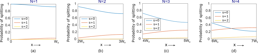
Figure 5: Probability amplitude splitting in optimally spaced (a) element-1, (b) element-2, (c) element-3, and (d) element-4 of optimally cascaded W-O converter, considering a classical wireless reception of field-strength $|E_{w}|$=50V/m.

The overall electro-optic modulation-depth $\delta\theta_{N}$ of the $N$-element array can be maximized if the time taken by the optical photon to travel between the respective entry points of two consecutive modulating elements is equal to the time-period of the received classical microwave E-field N. Ghosh and S. Pendharker (2023). This can only be achieved by optimally choosing the array periodicity as $D$=$D_{o}$=$(\pi c/\omega_{w}\sqrt{\epsilon_{op}}))$, which is twice the optimum element width $W_{o}$. The overall transmission matrix $[T]$ of the optimally cascaded array can be derived by putting $D$=$D_{o}$=$2W_{o}$ in the expression of $[T]$ mentioned in Eq. (63) of Appendix-D to be,

$$[T]=e^{-j\chi}\begin{bmatrix}\textbf{.}&\textbf{.}&\textbf{.}&\textbf{.}&\textbf{.}\\ \textbf{.}&\textbf{.}&\textbf{.}&\textbf{.}&\textbf{.}\\ \textbf{.}&J_{0}(\delta\theta_{No})&j^{-1}J_{-1}(\delta\theta_{No})e^{j(\omega_{w}t+\phi_{N}+b_{i})}&j^{-2}J_{-2}(\delta\theta_{No})e^{j2(\omega_{w}t+\phi_{N}+b_{i})}&\textbf{.}\\ \textbf{.}&jJ_{1}(\delta\theta_{No})e^{-j(\omega_{w}t+\phi_{N}+b_{i})}&J_{0}(\delta\theta_{No})&j^{-1}J_{-1}(\delta\theta_{No})e^{j(\omega_{w}t+\phi_{N}+b_{i})}&\textbf{.}\\ \textbf{.}&j^{2}J_{2}(\delta\theta_{No})e^{-j2(\omega_{w}t+\phi_{N}+b_{i})}&j^{1}J_{1}(\delta\theta_{No})e^{-j(\omega_{w}t+\phi_{N}+b_{i})}&J_{0}(\theta_{No})&\textbf{.}\\ \textbf{.}&\textbf{.}&\textbf{.}&\textbf{.}&\textbf{.}\\ \textbf{.}&\textbf{.}&\textbf{.}&\textbf{.}&\textbf{.}\end{bmatrix}$$ (18)

where the phase term $\chi$ in the above equation is,

$$\chi=(N-1)k_{op}D_{o}+k_{op}W$$ (19)

Also $\delta\theta_{No}$ is the overall maximized electro-optic modulation-depth of the optimally cascaded array expressed as,

$$\delta\theta_{No}=-N\frac{\omega_{op}\epsilon_{op}r_{33}}{\omega_{w}}\ \gamma|E_{w}|\ \sin{\bigg{(}\frac{\omega_{w}\sqrt{\epsilon_{op}}W}{2c}\bigg{)}}$$ (20)

Also the offset phase term $\phi_{N}$ in the matrix $[T]$ represented in Eq. (18) is,

$$\phi_{N}=\pi(N-1)+\frac{\omega_{w}\sqrt{\epsilon_{op}}W}{2c}$$ (21)

The total probability amplitude of the modulated optical photon at the output of the optimally cascaded $N$-element array, considering only the probability amplitude component $C^{0}_{1}$ to be present at the input can be derived to be (see Appendix-D),

$$\tilde{C_{1}}=C^{0}_{1}e^{-j(\omega_{op}t+\chi)}\sum_{s=-\infty}^{s=\infty}j^{s}J_{s}(\delta\theta_{No})e^{-js(\omega_{w}t+\phi_{N}+b_{i})}$$ (22)

Since, the electro-optic modulation-depth $\delta\theta_{N_{o}}$ gets upscaled in an optimally cascaded array, the probability amplitude splitting increases as the number of cascaded modulating elements are increased. Figure. 5 shows the increase in probability amplitude splitting of an optical photon modulated in a modulating-element array cascaded at an array periodicity $D_{o}$=$2W_{o}$=5.8$mm$ for a received 30GHz classical microwave carrier of field-strength $|E_{w}|$=50V/m.

By reversing Jacobi-Anger expansion in Eq. (22), we get the following expression for $\tilde{C}_{1}$,

$$\tilde{C}_{1}=C^{0}_{1}e^{-j(\omega_{op}t+\chi+\theta_{i}(t))}$$ (23)

where $\theta_{i}(t)$ is the phase encoded in the modulated optical photon and is related to the incident classical microwave digital phase $b_{i}$ as follows,

$$\theta_{i}(t)=\delta\theta_{No}\sin{\bigg{(}\omega_{w}t+\frac{\omega_{w}\sqrt{\epsilon_{op}}W}{2c}+b_{i}\bigg{)}}$$ (24)

In general, a modulated quantum optical state $\ket{\psi(t)}$ composed of a superposition of photon number-states can therefore be expressed as,

$$\ket{\psi(t)}=\sum_{k=0}^{k=\infty}C^{0}_{k}e^{-jk(\omega_{op}t+\chi+\theta_{i}(t))}\ket{k}$$ (25)

where $C^{0}_{k}$ is the initial probability amplitude of the $k^{th}$ photon number-state. In conclusion, the classical digital phase $b_{i}$ encoded in the received wireless microwave E-field gets mapped as the phase of the modulated quantum optical state $\theta_{i}(t)$ in the transduction process.

IV Quantum optical phase-space encoding with classical microwave constellation

In this section, we use our derived framework to investigate seamless encoding of quantum optical phase-space with digital constellation encapsulated in the received classical microwave carrier.

We consider an unmodulated optical coherent-state $\ket{\alpha}$ of mean complex amplitude $\alpha$ to be launched into an optimally cascaded $N$-element array of optimum width $W_{o}$. In the presence of classical microwave reception, the optical coherent-state undergoes electro-optic phase-modulation, as discussed previously. The modulated optical coherent-state $\ket{\alpha_{i}(t)}$ at the array output can be expressed as,

$$\ket{\alpha_{i}(t)}=\sum_{k=0}^{\infty}e^{-|\alpha|^{2}/2}\ \frac{\big{(}\alpha_{i}(t)\big{)}^{k}}{\sqrt{k!}}\ket{k}$$ (26)

where $\alpha_{i}(t)$=$\alpha e^{-j(\omega_{op}t+\theta_{i}(t))}$ is the time-varying mean complex amplitude of the modulated optical coherent-state at the output of the array. Here $\theta_{i}(t)$ is the mean optical phase encoded in $\ket{\alpha_{i}(t)}$ as it undergoes electro-optic modulation. Substituting the expression of $\theta_{i}(t)$ from Eq. (24) and putting $W$=$W_{o}$ into the expression of $\alpha_{i}(t)$ and expanding it using Jacobi-Anger expansion, we get the following,

$$\begin{split}\alpha_{i}(t)=\alpha e^{-j\omega_{op}t}\sum_{s=-\infty}^{s=\infty}(-1)^{s}J_{s}(\delta\theta_{N_{o}})\ e^{-js(\omega_{w}t+b_{i})}\end{split}$$ (27)

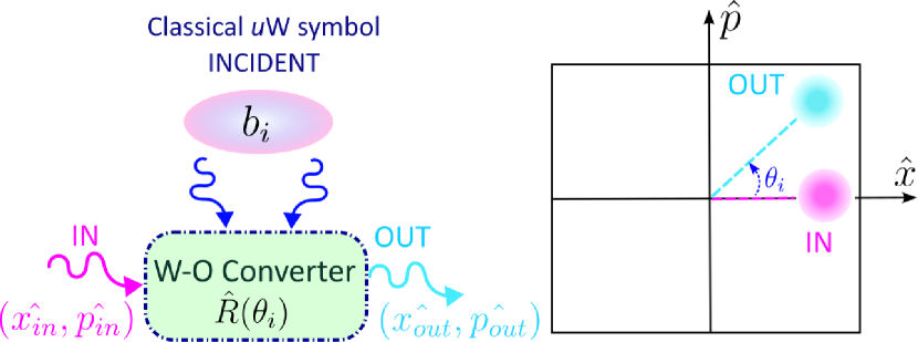
Figure 6: Unitary rotation operation of an optical coherent-state due to microwave-to-optical transduction.

For practical values of microwave E-field strength $|E_{w}|$, the electro-optic modulation-depth $\delta\theta_{N_{o}}$ is small enough such that higher-order sidebands ($s>1$) of the complex-amplitudes $\alpha_{i}(t)$ are negligible. Also since $\omega_{op}>>\omega_{w}$, it can be argued that sideband amplitudes in Eq. (27) approximately rotate around the origin of the $\hat{x}$-$\hat{p}$ phase-space at a frequency $\omega_{op}$. Therefore, the expansion in Eq. (27) leads to,

$$\begin{split}\alpha_{i}(t)&=\alpha e^{-j\omega_{op}t}\sum_{s=-\infty}^{s=\infty}(-1)^{s}J_{s}(\delta\theta_{N_{o}})\ e^{-jsb_{i}}\\ &=\alpha e^{-j(\omega_{op}t+\theta_{i})}\end{split}$$ (28)

where $\theta_{i}$ is the mean offset-phase encoded in the optical coherent-state due to electro-optic modulation. The phase $\theta_{i}$ is related to the $i^{th}$ digital microwave phase $b_{i}$ as follows,

$$\theta_{i}=-N\frac{\omega_{op}\epsilon_{op}r_{33}}{\omega_{w}}\ \gamma|E_{w}|\ \cos{b_{i}}$$ (29)

The time-independent mean complex amplitude of the modulated coherent-state can be expressed as $\alpha_{i}$=$\alpha e^{-j\theta_{i}}$. Therefore, the mean location of the modulated optical coherent-state in the $\hat{x}$-$\hat{p}$ phase-space is given by $<\hat{x}>$=$\Re{\{\alpha_{i}\}}$ and $<\hat{p}>$=$\Im{\{\alpha_{i}\}}$, which is in turn governed by the digital classical microwave phase $b_{i}$. This lays the foundation for digitally modulated classical microwave to quantum optical mapping.

It can also be shown that the variance in the phase-space location of the modulated optical coherent-state is independent of the received digital classical phase $b_{i}$ i.e. $\Delta\hat{x}$=$\Delta\hat{p}$=$1/2$, irrespective of the value of $b_{i}$. Therefore, it can be concluded that the discussed electro-optic interaction in the W-O converter only causes a unitary rotation of the coherent-state in the $\hat{x}$-$\hat{p}$ phase-space. Therefore, the quadrature operators $(\hat{x_{in}},\hat{p_{in}})$ of the unmodulated coherent-state at the input gets transformed to the quadrature operators $(\hat{x_{out}},\hat{p_{out}})$ at the output of the W-O converter, as shown in Fig. 6. The corresponding matrix transformation is given as,

$$\begin{pmatrix}\hat{x_{out}}\\ \hat{p_{out}}\\ \end{pmatrix}=\hat{R}(\theta_{i})\begin{pmatrix}\hat{x_{in}}\\ \hat{p_{in}}\\ \end{pmatrix}$$ (30)

The unitary rotation operator $\hat{R}(\theta_{i})$ in the above equation can be expressed as,

$$\hat{R}(\theta_{i})=\begin{pmatrix}\cos{(\theta_{i})}&-\sin{(\theta_{i})}\\ \sin{(\theta_{i})}&\cos{(\theta_{i})}\\ \end{pmatrix}$$ (31)

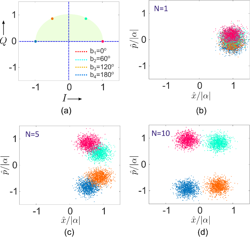
Figure 7: (a) Received classical 30GHz modified 4-ary PSK constellation of field-strength $|E_{w}|$=50V/m. Correspondingly encoded phase-space of the optical coherent-state consisting of mean photon numbers $\tilde{n}_{ph}$=10 at the output of a (b) single-element, (c) 5-element, and (d) 10-element optimally cascaded array.

Figure 7(a) represents the received constellation of a modified 4-ary PSK constellation Ghosh and Pendharker (2021) with possible digital phase-levels $b_{i}$ = $\{0^{\circ},60^{\circ},120^{\circ},180^{\circ}\}$, encapsulated in a 30GHz classical wireless microwave carrier of field-strength $|E_{w}|$=50V/m. The correspondingly encoded phase-space of the modulated optical coherent-state consisting of mean photon numbers $\tilde{n}_{ph}$=$|\alpha|^{2}$=10 at the output of a W-O converter is shown in Fig 7(b)-(d). It can be observed that each digital phase $b_{i}$ encapsulated in the received microwave constellation gets mapped to a particular location in the quantum optical phase-space. This leads to the encoding of quantum optical phase-space with the received classical microwave constellation.

It must also be pointed out that there is a high probability of overlap between different symbols in the encoded quantum optical phase-space due to quantum optical shot noise. This poses the challenge of indistinguishability between different encoded symbols in the quantum optical phase-space. However, this overlap can be significantly reduced by spacing out the mean locations of each optical symbols away from each other in the phase-space. This can be achieved by increasing the number of optimally cascaded modulating elements in the W-O converter, as shown in Fig 7(c)-(d), the physical reason of which was discussed in the previous section.

It can also be observed from Fig 8 that the inter-symbol overlap in the quantum optical phase-space decreases as the mean photon numbers in the optical coherent-states decrease. This happens due to the decrease in the relative variance of the symbol locations in the quantum optical phase-space as the mean optical photon number is increased.

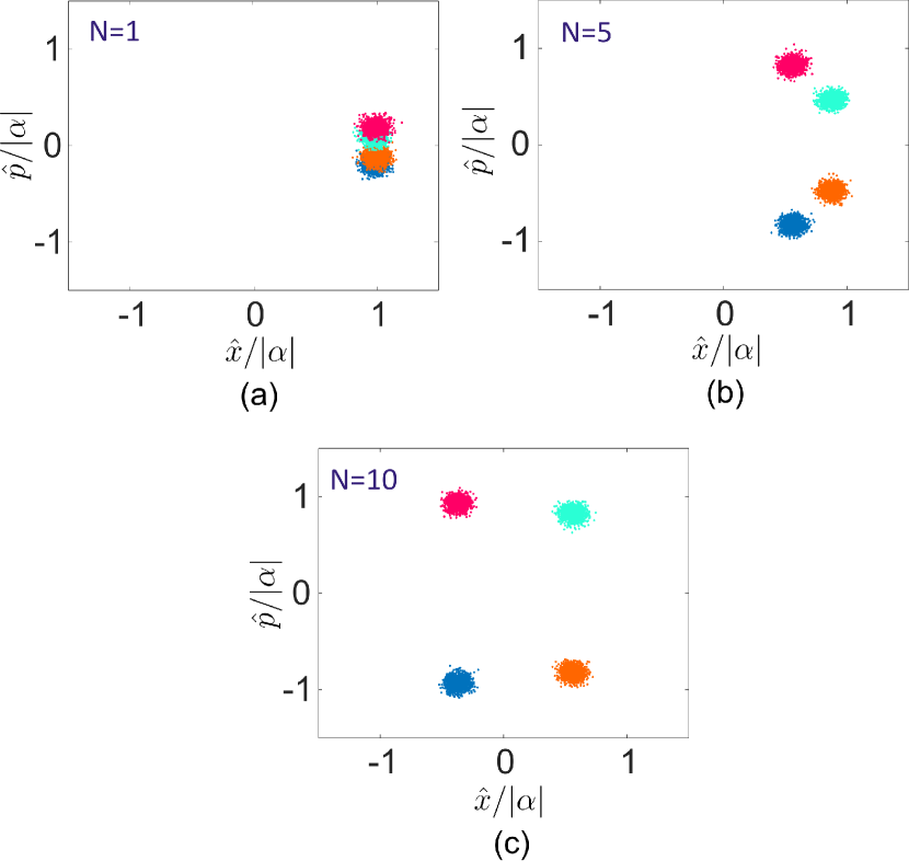
Figure 8: Modulated phase-space of the optical coherent-state of mean photon numbers $\tilde{n}_{ph}$=100 at the output of a (a) single-element, (b) 5-element, and (c) 10-element optimally cascaded array.

V Conclusion

In this paper, we investigated seamless transduction digital information encoded in the classical microwave domain to the quantum optical domain. We introduced a quantum mechanical framework model that can be used to understand and visualize the electro-optic interaction between quantum state of light and a digitally modulated classical microwave signal in the transduction process. Enhancement of electro-optic interaction strength through suitable choices of certain physical parameters such as individual modulating-element width and inter-element spacing, have been discussed and supported by physical reasoning. Interestingly, we showed that the phase-space of a quantum optical state can be manipulated by the digital information encoded within the received classical microwave constellation. This essentially forms the basis for potentially bridging classical wireless and quantum optical links in the future. The challenge of intersymbol overlap in the encoded quantum optical phase-space due to shot noise has also been pointed out, and its mitigation been discussed. The general framework of microwave-to-optical transduction presented in this paper can further be extended to explore the interesting cases for single-photons, squeezed-states, and other non-classical states of light that will have a wide range of applications in both continuous and discrete-variable quantum computing and networking in the future.

Appendix A Derivation of the electro-optic interaction Hamiltonian

The Pockel’s electro-optic effect governed interaction Hamiltonian $\hat{H_{I}}(t)$ associated with a quantum optical mode propagating in the waveguide routed through a modulating element receiving a classical microwave E-field $E_{w}(t)$ is,

$$\hat{H}_{I}(t)=\int_{V}\frac{1}{2}\ \epsilon_{o}\ \delta\epsilon_{op}(t)\ \hat{E}_{op}{(t)}.\hat{E}_{op}{(t)}\ dV$$ (32)

where $\delta\epsilon_{op}(t)$ is the Pockel’s effect induced perturbation in the relative permittivity of the optical waveguide. By substituting the expression of $\delta\epsilon_{op}(t)$ from Eq. (4) and the expression of $\hat{E}_{op}(t)$ from Eq. (1) in the above integral, we get,

$$\hat{H}_{I}(t) =\frac{\hbar\omega_{op}}{4V}\ \epsilon_{op}r_{33}E_{w}(t)\ \int_{V}\big{(}\hat{a}.\hat{a}\ e^{-i2(\omega_{op}t-k_{op}z)}$$ (33)

$$-\hat{a}.\hat{a}^{\dagger}-\hat{a}^{\dagger}.\hat{a}+\hat{a}^{\dagger}.\hat{a}^{\dagger}\ e^{i2(\omega_{op}t-k_{op}z)}\big{)}\ dV$$

The result of integrating the terms $\hat{a}.\hat{a}\ e^{-i2(\omega_{op}t-k_{op}z)}$ and $\hat{a}^{\dagger}.\hat{a}^{\dagger}\ e^{i2(\omega_{op}t-k_{op}z)}$ becomes zero on applying periodic boundary-condition in the above integral Gerry and Knight (2023). Consequently, the integral of Eq. (33) simplifies down to,

$$\hat{H_{I}}(t)=-\frac{\epsilon_{op}r_{33}}{2}\gamma E_{w}(t)\ \hbar\omega_{op}\big{(}\hat{a}^{\dagger}\hat{a}+\frac{1}{2}\big{)}$$ (34)

For the sake of simplicity, we consider the reference vacuum eigen energy of the quantum optical mode to be zero. In such a case, the interaction Hamiltonian $\hat{H_{I}}(t)$ simplifies to,

$$\hat{H_{I}}(t)=-\frac{\epsilon_{op}r_{33}}{2}\gamma E_{w}(t)\ \hbar\omega_{op}\hat{a}^{\dagger}\hat{a}$$ (35)

Therefore, the total Hamiltonian of the quantum optical mode can be expressed as,

$$\begin{split}\hat{H}&=\hat{H_{o}}+\hat{H}_{I}(t)\\ &=\hbar\omega_{op}\hat{a}^{\dagger}\hat{a}-\frac{\epsilon_{op}r_{33}}{2}\gamma E_{w}(t)\ \hbar\omega_{op}\hat{a}^{\dagger}\hat{a}\end{split}$$ (36)

Appendix B Derivation of time-evolution of a single optical photon state in the modulating element

The time-evolving probability amplitude $C_{1}(t)$ associated with a single optical photon state due to electro-optic interaction with the received classical microwave E-field during the time window $t$ to $(t+T_{W})$ can be found by integrating Eq. (10) as follows,

$$\int_{t}^{t+T_{W}}\frac{dC_{1}(t)}{C_{1}(t)}=-j\int_{t}^{t+T_{W}}\omega_{op}\bigg{(}1-\frac{\epsilon_{op}r_{33}}{2}\ \gamma E_{w}(t)\bigg{)}dt$$ (37)

Substituting the expression of $E_{w}(t)$ from Eq. (3) and putting $T_{W}$=$(W\sqrt{\epsilon_{op}}/c)$ in the above integral,we solve it to get,

$$C_{1}(t+T_{W})=C_{1}(t)e^{-jk_{op}W}e^{-j\delta\theta\sin{(\omega_{w}t+\phi+b_{i})}}$$ (38)

where $C_{1}(t+T_{W})$ and $C_{1}(t)$ are the output and input probability amplitudes of the single optical photon state at the instants $(t+T_{W})$ and $t$, respectively. Also, $C_{1}(t)$=$C_{1}(0)e^{-j\omega_{op}t}$, where $C_{1}(0)$ is the initial probability amplitude of the photon state at $t$=0. For the sake of notational simplicity, we represent $C_{1}(t+T_{W})$ as $\tilde{C_{1}}$, and $C_{1}(0)$ as $C_{1}$ from now on. Therefore, the time-evolving probability amplitude $C_{1}(t)$ can be expressed as,

$$\tilde{C}_{1}=C_{1}\ e^{-j(\omega_{op}t+k_{op}W+\delta\theta\sin{(\omega_{w}t+\phi+b_{i})})}$$ (39)

where the expressions of $\delta\theta$ and $\phi$ are mentioned in Eq. (13) and Eq. (14), respectively. Expanding Eq. (39) using Jacobi-Anger expansion, we get the following expression,

$$\tilde{C_{1}}=C_{1}e^{-j(\omega_{op}t+k_{op}W)}\sum^{s=\infty}_{s=-\infty}j^{s}J_{s}(\delta\theta)\ e^{-js({\omega_{w}}t+\phi+b_{i})}$$ (40)

where $\delta\theta$ represents the electro-optic modulation-depth, which can be expressed as follows,

$$\delta\theta=-\frac{\omega_{op}\epsilon_{op}r_{33}}{\omega_{w}}\ \gamma|E_{w}|\ \sin{\bigg{(}\frac{\omega_{w}\sqrt{\epsilon_{op}}W}{2c}\bigg{)}}$$ (41)

Also the offset phase term $\phi$ can be expressed as,

$$\phi=\frac{\omega_{w}\sqrt{\epsilon_{op}}W}{2c}$$ (42)

It can be concluded that the probability amplitude of the modulated optical photon state splits into different sideband components. Therefore, the output probability amplitude vector $[\tilde{C^{s}_{1}}]$ and the input probability amplitude vector $[{C^{s}_{1}}]$ are related by the matrix relation $[\tilde{C^{s}_{1}}]$=$[T][{C^{s}_{1}}]$, where the transmission matrix $[T]$ can be expressed as,

$$[T]=e^{-jk_{op}W}\begin{bmatrix}\textbf{.}&\textbf{.}&\textbf{.}&\textbf{.}&\textbf{.}&\textbf{.}&\textbf{.}\\ \textbf{.}&\textbf{.}&\textbf{.}&\textbf{.}&\textbf{.}&\textbf{.}&\textbf{.}\\ \textbf{.}&\textbf{.}&J_{0}(\delta\theta)&j^{-1}J_{-1}(\delta\theta)e^{j(\omega_{w}t+\phi+b_{i})}&j^{-2}J_{-2}(\delta\theta)e^{j2(\omega_{w}t+\phi+b_{i})}&\textbf{.}&\textbf{.}\\ \textbf{.}&\textbf{.}&jJ_{1}(\delta\theta)e^{-j(\omega_{w}t+\phi+b_{i})}&J_{0}(\delta\theta)&j^{-1}J_{-1}(\delta\theta)e^{j(\omega_{w}t+\phi+b_{i})}&\textbf{.}&\textbf{.}\\ \textbf{.}&\textbf{.}&j^{2}J_{2}(\delta\theta)e^{-j2(\omega_{w}t+\phi+b_{i})}&j^{1}J_{1}(\delta\theta)e^{-j(\omega_{w}t+\phi+b_{i})}&J_{0}(\delta\theta)&\textbf{.}&\textbf{.}\\ \textbf{.}&\textbf{.}&\textbf{.}&\textbf{.}&\textbf{.}&\textbf{.}&\textbf{.}\\ \textbf{.}&\textbf{.}&\textbf{.}&\textbf{.}&\textbf{.}&\textbf{.}&\textbf{.}\end{bmatrix}$$ (43)

Appendix C Optimum and non-optimum modulating element width

The transmission matrix $[T^{(m=1)}]$ of the equivalent quantum mechanical network associated with the modulating section $m$=$1$ of width $W_{o}$ represented in Fig. 3(a), can be derived by integrating Eq. (37) in the time window $t$ to $(t+T_{W_{o}})$. Here, $T_{W_{o}}$=$(W_{o}\sqrt{\epsilon_{op}}/c)$ is the time taken by the optical photon state to travel distance $W_{o}$ in the waveguide. Following the procedure shown in the previous section, the transmission matrix $[T^{(m=1)}]$ associated with the modulating section $m$=1 in Fig. 3(a) is,

$$[T^{(m=1)}]=e^{-jk_{op}W_{o}}\begin{bmatrix}\textbf{.}&\textbf{.}&\textbf{.}&\textbf{.}&\textbf{.}&\textbf{.}&\textbf{.}\\ \textbf{.}&\textbf{.}&\textbf{.}&\textbf{.}&\textbf{.}&\textbf{.}&\textbf{.}\\ \textbf{.}&\textbf{.}&J_{0}(\delta\theta_{o})&j^{-1}J_{-1}(\delta\theta_{o})e^{j(\omega_{w}t+\pi/2+b_{i})}&j^{-2}J_{-2}(\delta\theta_{o})e^{j2(\omega_{w}t+\pi/2+b_{i})}&\textbf{.}&\textbf{.}\\ \textbf{.}&\textbf{.}&jJ_{1}(\delta\theta_{o})e^{-j(\omega_{w}t+\pi/2+b_{i})}&J_{0}(\delta\theta_{o})&j^{-1}J_{-1}(\delta\theta_{o})e^{j(\omega_{w}t+\pi/2+b_{i})}&\textbf{.}&\textbf{.}\\ \textbf{.}&\textbf{.}&j^{2}J_{2}(\delta\theta_{o})e^{-j2(\omega_{w}t+\pi/2+b_{i})}&j^{1}J_{1}(\delta\theta_{o})e^{-j(\omega_{w}t+\pi/2+b_{i})}&J_{0}(\delta\theta_{o})&\textbf{.}&\textbf{.}\\ \textbf{.}&\textbf{.}&\textbf{.}&\textbf{.}&\textbf{.}&\textbf{.}&\textbf{.}\\ \textbf{.}&\textbf{.}&\textbf{.}&\textbf{.}&\textbf{.}&\textbf{.}&\textbf{.}\end{bmatrix}$$ (44)

where $\delta\theta_{o}$=$-(\omega_{op}\epsilon_{op}r_{33}/\omega_{w})\gamma|E_{w}|$ is the electro-optic modulation depth of the modulating section $m$=1. Similarly, the transmission matrix $[T^{(m=2)}]$ of the equivalent quantum mechanical network associated with the modulating section $m$=$2$, also having width $W_{o}$ as illustrated in Fig. 3(a), can be derived by integrating Eq. (37) in the time window $(t+T_{W_{o}})$ to $(t+2T_{W_{o}})$ to get the following,

$$[T^{(m=2)}]=e^{-jk_{op}W_{o}}\begin{bmatrix}\textbf{.}&\textbf{.}&\textbf{.}&\textbf{.}&\textbf{.}&\textbf{.}&\textbf{.}\\ \textbf{.}&\textbf{.}&\textbf{.}&\textbf{.}&\textbf{.}&\textbf{.}&\textbf{.}\\ \textbf{.}&\textbf{.}&J_{0}(\delta\theta_{o})&j^{-1}J_{-1}(\delta\theta_{o})e^{j(\omega_{w}t+3\pi/2+b_{i})}&j^{-2}J_{-2}(\delta\theta_{o})e^{j2(\omega_{w}t+3\pi/2+b_{i})}&\textbf{.}&\textbf{.}\\ \textbf{.}&\textbf{.}&jJ_{1}(\delta\theta_{o})e^{-j(\omega_{w}t+3\pi/2+b_{i})}&J_{0}(\delta\theta_{o})&j^{-1}J_{-1}(\delta\theta_{o})e^{j(\omega_{w}t+3\pi/2+b_{i})}&\textbf{.}&\textbf{.}\\ \textbf{.}&\textbf{.}&j^{2}J_{2}(\delta\theta_{o})e^{-j2(\omega_{w}t+3\pi/2+b_{i})}&j^{1}J_{1}(\delta\theta_{o})e^{-j(\omega_{w}t+3\pi/2+b_{i})}&J_{0}(\delta\theta_{o})&\textbf{.}&\textbf{.}\\ \textbf{.}&\textbf{.}&\textbf{.}&\textbf{.}&\textbf{.}&\textbf{.}&\textbf{.}\\ \textbf{.}&\textbf{.}&\textbf{.}&\textbf{.}&\textbf{.}&\textbf{.}&\textbf{.}\end{bmatrix}$$ (45)

It can be easily shown that the derived transmission matrices $[T^{(m=1)}]$ and $[T^{(m=2)}]$ are related as,

$$[T^{(m=1)}]=e^{-j2k_{op}W_{o}}[T^{(m=2)}]^{\dagger}$$ (46)

Also, since the transmission matrices $[T^{(m=1)}]$ and $[T^{(m=2)}]$ are unitary, it can be further shown that they are related to each other by the following relationship,

$$[T^{(m=1)}]=e^{-j2k_{op}W_{o}}[T^{(m=2)}]^{-1}$$ (47)

The overall transmission matrix $[T]$ of the modulating element of width $W$=$2W_{o}$, which is essentially the cascade of the modulating sections $m$=1 and $m$=2, is equal to the product of the matrices $[T^{(m=1)}]$ and $[T^{(m=2)}]$. Therefore, the overall transmission matrix $[T]$ can be derived to be the following,

$$[T]=[T^{(m=2)}][T^{(m=1)}]=e^{-j2k_{op}W_{o}}[\mathcal{I}]$$ (48)

Appendix D Transmission matrix for multiple modulating element based W-O converter

The transmission matrix of the $n^{th}$ modulating element in the array represented in Fig. 4(b) can be derived by integrating Eq. (37) in the time window $(t+(n-1)T_{D})$ to $(t+(n-1)T_{D}+T_{W})$. Here, $T_{D}$=$D\sqrt{\epsilon_{op}}/c$ is the time taken by the optical photon state to travel distance $D$ in the optical waveguide. The transmission matrix of the $[T^{n}]$ can then be derived to be,

$$[T^{n}]=e^{-jk_{op}W}\begin{bmatrix}\textbf{.}&\textbf{.}&\textbf{.}&\textbf{.}&\textbf{.}&\textbf{.}&\textbf{.}\\ \textbf{.}&\textbf{.}&\textbf{.}&\textbf{.}&\textbf{.}&\textbf{.}&\textbf{.}\\ \textbf{.}&\textbf{.}&J_{0}(\delta\theta)&j^{-1}J_{-1}(\delta\theta)e^{j(\omega_{w}t+\phi_{n}+b_{i})}&j^{-2}J_{-2}(\delta\theta)e^{j2(\omega_{w}t+\phi_{n}+b_{i})}&\textbf{.}&\textbf{.}\\ \textbf{.}&\textbf{.}&jJ_{1}(\delta\theta)e^{-j(\omega_{w}t+\phi_{n}+b_{i})}&J_{0}(\delta\theta)&j^{-1}J_{-1}(\delta\theta)e^{j(\omega_{w}t+\phi_{n}+b_{i})}&\textbf{.}&\textbf{.}\\ \textbf{.}&\textbf{.}&j^{2}J_{2}(\delta\theta)e^{-j2(\omega_{w}t+\phi_{n}+b_{i})}&j^{1}J_{1}(\delta\theta)e^{-j(\omega_{w}t+\phi_{n}+b_{i})}&J_{0}(\delta\theta)&\textbf{.}&\textbf{.}\\ \textbf{.}&\textbf{.}&\textbf{.}&\textbf{.}&\textbf{.}&\textbf{.}&\textbf{.}\\ \textbf{.}&\textbf{.}&\textbf{.}&\textbf{.}&\textbf{.}&\textbf{.}&\textbf{.}\end{bmatrix}$$ (49)

where the offset phase $\phi_{n}$ in the above matrix is,

$$\phi_{n}=\frac{\omega_{w}\sqrt{\epsilon_{op}}W}{2c}+(n-1)\frac{\omega_{w}\sqrt{\epsilon_{op}}D}{c}$$ (50)

It must be pointed out that no electro-optic interaction takes place in the optical waveguide segment placed between the $n^{th}$ and the $(n+1)^{th}$ modulating element. The length of each such segment is equal to $G$=$(D-W)$, and thus can be modeled as an infinite-port network of identity transmission matrix having the following form,

$$[\mathcal{I}^{n}]=e^{-jk_{op}G}[\mathcal{I}]$$ (51)

Therefore, the overall transmission matrix of the modulating array composed of $N$ modulating elements of width $W$, cascaded at an array periodicity $D$, can be derived to be,

$$[T]=[T^{N}]\prod_{n=1}^{n=(N-1)}[\mathcal{I}^{n}][T^{n}]$$ (52)

It can be shown that the matrix element $T_{sp}$ belonging to the $s^{th}$ row and $p^{th}$ column of the transmission matrix $[T]$ is equal to,

$$\small T_{sp}=e^{-jk_{op}((N-1)D+W)}\sum_{x_{n}}\prod_{n=1}^{n=N}j^{x_{n}}J_{x_{n}}(\delta\theta)e^{-jx_{n}(\omega_{w}t+\phi_{n}+b_{i})}$$ (53)

where $\sum_{n=1}^{N}x_{n}=(s-p)$ in the above expression. From the derived transmission matrix $[T]$, the $s^{th}$ sideband component of the output probability amplitude $\tilde{C^{s}_{1}}$ can be found out to be,

$$\tilde{C^{s}_{1}}=\sum_{p=-\infty}^{p=\infty}T_{sp}\ C^{p}_{1}$$ (54)

where $C^{p}_{1}$ is the $p^{th}$ sideband component of the probability amplitude of the optical photon state at the input of the array. If we only consider the fundamental frequency component of the probability amplitude $C^{p=0}_{1}$=$C_{1}e^{-j\omega_{op}t}$ of the optical photon state at the input of the array, the expression of $\tilde{C^{s}_{1}}$ in Eq. (54) becomes equal to the following,

$$\tilde{C^{s}_{1}}=T_{s0}\ C^{0}_{1}$$ (55)

Substituting the expression of $T_{sp}$ for $p$=0 from Eq. (53) into the above equation, we get,

$$\begin{split}\tilde{C^{s}_{1}}&=e^{-j(\omega_{op}t+(N-1)k_{op}D+k_{op}W)}\sum_{x_{n}}\big{(}\prod_{n=1}^{n=N}\\ &j^{x_{n}}J_{x_{n}}(\delta\theta)\ e^{-jx_{n}(\omega_{w}t+\phi_{n}+b_{i})}\ C^{0}_{1}\big{)}\end{split}$$

where in this case, we have $\sum_{n=1}^{N}x_{n}=s$. Now, taking the summation of all the components present in the output probability amplitude vector $[\tilde{C_{1}}(s)]$, we get the total probability amplitude of the modulated optical photon state at the output of the array as,

$$\begin{split}\tilde{C_{1}}&=\sum_{s=-\infty}^{s=\infty}\tilde{C}_{1}(s)\\ &=e^{-j(\omega_{op}t+(N-1)k_{op}D+k_{op}W)}\sum_{s=-\infty}^{s=\infty}\big{(}\sum_{x_{n}}\prod_{n=1}^{n=N}j^{x_{n}}J_{x_{n}}(\delta\theta)\ e^{-jx_{n}(\omega_{w}t+\phi_{n}+b_{i})}\big{)}\ C^{0}_{1}\\ &=e^{-j(\omega_{op}t+(N-1)k_{op}D+k_{op}W)}\prod_{n=1}^{n=N}\big{(}\sum_{s=-\infty}^{s=\infty}j^{s}J_{s}(\delta\theta)\ e^{-js(\omega_{w}t+\phi_{n}+b_{i})}\big{)}\ C^{0}_{1}\\ &=e^{-j(\omega_{op}t+(N-1)k_{op}D+k_{op}W)}\prod_{n=1}^{n=N}e^{-j\delta\theta\sin{(\omega_{w}t+\phi_{n}+b_{i})}}\ C^{0}_{1}\\ &=e^{-j(\omega_{op}t+(N-1)k_{op}D+k_{op}W)}\exp{\bigg{(}-j\sum_{n=1}^{n=N}\delta\theta\sin{(\omega_{w}t+\phi_{n}+b_{i})}\bigg{)}}\ C^{0}_{1}\end{split}$$ (56)

By substituting the expression of $\delta\theta$ and $\phi_{n}$ to Eq. (56), we can simplify the summation series in Eq. (56) in the following manner,

$$\begin{split}\sum_{n=1}^{n=N}\delta\theta\sin{(\omega_{w}t+\phi_{n}+b_{i})}&=\sum_{n=1}^{n=N}\delta\theta\sin{\bigg{(}\omega_{w}t+\frac{\omega_{w}D\sqrt{\epsilon_{op}}}{2c}+(n-1)\frac{\omega_{w}D\sqrt{\epsilon_{op}}}{c}+b_{i}\bigg{)}}\\ &=\delta\theta\frac{\sin{(N\omega_{w}\sqrt{\epsilon_{op}}D/2)}}{\sin{(\omega_{w}\sqrt{\epsilon_{op}}D/2)}}\sin{\bigg{(}\omega_{w}t+\frac{\omega_{w}W\sqrt{\epsilon_{op}}}{2c}+(N-1)\frac{\omega_{w}D\sqrt{\epsilon_{op}}}{2c}+b_{i}\bigg{)}}\\ &=\delta\theta_{N}\sin{(\omega_{w}t+\phi_{N}+b_{i})}\end{split}$$ (57)

where $\delta\theta_{N}$ in the above equation is the overall electro-optic modulation-depth of the $N$-element array,

$$\delta\theta_{N}=\delta\theta\frac{\sin{(N\omega_{w}\sqrt{\epsilon_{op}}D/2)}}{\sin{(\omega_{w}\sqrt{\epsilon_{op}}D/2)}}$$ (58)

Also, the offset phase term $\phi_{N}$ can be expressed as,

$$\phi_{N}=\frac{\omega_{w}D\sqrt{\epsilon_{op}}}{2c}+(N-1)\frac{\omega_{w}\sqrt{\epsilon_{op}}D}{2c}$$ (59)

Therefore, the total output probability amplitude $\tilde{C_{1}}$ of the modulated optical photon state at the output of the modulating array becomes,

$$\tilde{C_{1}}=C^{0}_{1}e^{-j(\omega_{op}t+\chi)}e^{-j\delta\theta_{N}\sin{(\omega_{w}t+\phi_{N}+b_{i})}}$$ (60)

Expanding the above expression using Jacobi-Anger expansion, we get the following,

$$\tilde{C_{1}}=C^{0}_{1}e^{-j(\omega_{op}t+\chi)}\sum_{s=-\infty}^{s=\infty}j^{s}J_{s}(\delta\theta_{N})e^{-js(\omega_{w}t+\phi_{N}+b_{i})}$$ (61)

where $\chi$ in the above equation is a constant phase term expressed as,

$$\chi=(N-1)k_{op}D+k_{op}W$$ (62)

Therefore, the overall transmission matrix $[T]$ relating the input and output probability amplitude components of the optical photon state in the $N$-element array can be derived to be,

$$[T]=e^{-j\chi}\begin{bmatrix}\textbf{.}&\textbf{.}&\textbf{.}&\textbf{.}&\textbf{.}&\textbf{.}&\textbf{.}\\ \textbf{.}&\textbf{.}&\textbf{.}&\textbf{.}&\textbf{.}&\textbf{.}&\textbf{.}\\ \textbf{.}&\textbf{.}&J_{0}(\delta\theta_{N})&j^{-1}J_{-1}(\delta\theta_{N})e^{j(\omega_{w}t+\phi_{N}+b_{i})}&j^{-2}J_{-2}(\delta\theta_{N})e^{j2(\omega_{w}t+\phi_{N}+b_{i})}&\textbf{.}&\textbf{.}\\ \textbf{.}&\textbf{.}&jJ_{1}(\delta\theta_{N})e^{-j(\omega_{w}t+\phi_{N}+b_{i})}&J_{0}(\delta\theta_{N})&j^{-1}J_{-1}(\delta\theta_{N})e^{j(\omega_{w}t+\phi_{N}+b_{i})}&\textbf{.}&\textbf{.}\\ \textbf{.}&\textbf{.}&j^{2}J_{2}(\delta\theta_{N})e^{-j2(\omega_{w}t+\phi_{N}+b_{i})}&j^{1}J_{1}(\delta\theta_{N})e^{-j(\omega_{w}t+\phi_{N}+b_{i})}&J_{0}(\delta\theta_{N})&\textbf{.}&\textbf{.}\\ \textbf{.}&\textbf{.}&\textbf{.}&\textbf{.}&\textbf{.}&\textbf{.}&\textbf{.}\\ \textbf{.}&\textbf{.}&\textbf{.}&\textbf{.}&\textbf{.}&\textbf{.}&\textbf{.}\end{bmatrix}$$ (63)

References

- Sahu et al. (2022) R. Sahu, W. Hease, A. Rueda, G. Arnold, L. Qiu, and J. M. Fink, Nature communications 13, 1276 (2022).
- Blümel et al. (2021) R. Blümel, N. Grzesiak, N. H. Nguyen, A. M. Green, M. Li, A. Maksymov, N. M. Linke, and Y. Nam, Physical Review Letters 126, 220503 (2021).
- Ringbauer et al. (2022) M. Ringbauer, M. Meth, L. Postler, R. Stricker, R. Blatt, P. Schindler, and T. Monz, Nature Physics 18, 1053 (2022).
- Covey et al. (2023) J. P. Covey, H. Weinfurter, and H. Bernien, npj Quantum Information 9, 90 (2023).
- Park et al. (2022) A. J. Park, J. Trautmann, N. Šantić, V. Klüsener, A. Heinz, I. Bloch, and S. Blatt, PRX Quantum 3, 030314 (2022).
- Hendrickx et al. (2020) N. Hendrickx, W. Lawrie, L. Petit, A. Sammak, G. Scappucci, and M. Veldhorst, Nature communications 11, 3478 (2020).
- Blumoff et al. (2022) J. Z. Blumoff, A. S. Pan, T. E. Keating, R. W. Andrews, D. W. Barnes, T. L. Brecht, E. T. Croke, L. E. Euliss, J. A. Fast, C. A. Jackson, et al., PRX Quantum 3, 010352 (2022).
- Krantz et al. (2019) P. Krantz, M. Kjaergaard, F. Yan, T. P. Orlando, S. Gustavsson, and W. D. Oliver, Applied physics reviews 6 (2019).
- Liu et al. (2020) C. Liu, T.-X. Zhu, M.-X. Su, Y.-Z. Ma, Z.-Q. Zhou, C.-F. Li, and G.-C. Guo, Physical Review Letters 125, 260504 (2020).
- Wu et al. (2020a) B.-H. Wu, R. N. Alexander, S. Liu, and Z. Zhang, Physical Review Research 2, 023138 (2020a).
- Han et al. (2021) X. Han, W. Fu, C.-L. Zou, L. Jiang, and H. X. Tang, Optica 8, 1050 (2021).
- Mirhosseini et al. (2020) M. Mirhosseini, A. Sipahigil, M. Kalaee, and O. Painter, Nature 588, 599 (2020).
- Fu et al. (2021) W. Fu, M. Xu, X. Liu, C.-L. Zou, C. Zhong, X. Han, M. Shen, Y. Xu, R. Cheng, S. Wang, et al., Physical Review A 103, 053504 (2021).
- Soltani et al. (2017) M. Soltani, M. Zhang, C. Ryan, G. J. Ribeill, C. Wang, and M. Loncar, Physical Review A 96, 043808 (2017).
- Rueda et al. (2016) A. Rueda, F. Sedlmeir, M. C. Collodo, U. Vogl, B. Stiller, G. Schunk, D. V. Strekalov, C. Marquardt, J. M. Fink, O. Painter, et al., Optica 3, 597 (2016).
- Xie et al. (2023) J. Xie, S. Ma, Y. Ren, X. Li, S. Gao, and F. Li, New Journal of Physics 25, 073009 (2023).
- Zhu et al. (2020) N. Zhu, X. Zhang, X. Han, C.-L. Zou, C. Zhong, C.-H. Wang, L. Jiang, and H. X. Tang, Optica 7, 1291 (2020).
- Zhang et al. (2016) X. Zhang, N. Zhu, C.-L. Zou, and H. X. Tang, Physical review letters 117, 123605 (2016).
- Kumar et al. (2023) A. Kumar, A. Suleymanzade, M. Stone, L. Taneja, A. Anferov, D. I. Schuster, and J. Simon, Nature 615, 614 (2023).
- Liao et al. (2023) K.-Y. Liao, H. Yan, and S.-L. Zhu, Nature Photonics , 1 (2023).
- Adwaith et al. (2019) K. Adwaith, A. Karigowda, C. Manwatkar, F. Bretenaker, and A. Narayanan, Optics Letters 44, 33 (2019).
- Kim et al. (2023) B. Kim, H. Kurokawa, K. Sakai, K. Koshino, H. Kosaka, and M. Nomura, Physical Review Applied 20, 044037 (2023).
- Zhong et al. (2022) C. Zhong, X. Han, and L. Jiang, Physical Review Applied 18, 054061 (2022).
- Wu et al. (2020b) M. Wu, E. Zeuthen, K. C. Balram, and K. Srinivasan, Physical review applied 13, 014027 (2020b).
- Xu et al. (2021) Y. Xu, A. A. Sayem, L. Fan, C.-L. Zou, S. Wang, R. Cheng, W. Fu, L. Yang, M. Xu, and H. X. Tang, Nature communications 12, 4453 (2021).
- Capmany and Fernández-Pousa (2010) J. Capmany and C. R. Fernández-Pousa, JOSA B 27, A119 (2010).
- Horoshko et al. (2018) D. Horoshko, M. Eskandary, and S. Y. Kilin, JOSA B 35, 2744 (2018).
- Pratap and Ramachandran (2020) R. Pratap and H. Ramachandran, JOSA B 37, 3016 (2020).
- Pratap and Ramachandran (2023) R. Pratap and H. Ramachandran, Journal of Optics (2023).
- Imany et al. (2018) P. Imany, O. D. Odele, J. A. Jaramillo-Villegas, D. E. Leaird, and A. M. Weiner, Physical Review A 97, 013813 (2018).
- Haykin (1988) S. Haykin, New York (1988).
- Ghosh and Pendharker (2021) N. Ghosh and S. Pendharker, Journal of Optics 23, 125702 (2021).
- N. Ghosh and S. Pendharker (2023) N. Ghosh and S. Pendharker, Journal of Lightwave Technology 41, 5851 (2023).
- Ghosh and Pendharker (2023) N. Ghosh and S. Pendharker, (2023).
- Gerry and Knight (2023) C. C. Gerry and P. L. Knight, Introductory quantum optics (Cambridge university press, 2023).
- Bransden (2000) B. H. Bransden, Quantum mechanics (Pearson Education India, 2000).